A Semi-Blind Method for Localization of Underwater Acoustic Sources

Amir Weiss, Toros Arikan, Hari Vishnu, Grant B. Deane, Andrew C. Singer, and Gregory W. Wornell This work was supported, in part, by ONR under Grant Nos. N00014-19-1-2661, N00014-19-1-2662, and N00014-19-1-2665, and NSF under Grant No. CCF-1816209.This paper has supplementary material available at http://weissamir.com, provided by the authors. The material includes: (i) technical derivations; (ii) details on the experiment; and (iii) a MATLAB code implementation of the proposed localization method, and computation of the performance bound.
Abstract

Underwater acoustic localization has traditionally been challenging due to the presence of unknown environmental structure and dynamic conditions. The problem is richer still when such structure includes occlusion, which causes the loss of line-of-sight (LOS) between the acoustic source and the receivers, on which many of the existing localization algorithms rely. We develop a semi-blind passive localization method capable of accurately estimating the source’s position even in the possible absence of LOS between the source and all receivers. Based on typically-available prior knowledge of the water surface and bottom, we derive a closed-form expression for the optimal estimator under a multi-ray propagation model, which is suitable for shallow-water environments and high-frequency signals. By exploiting a computationally efficient form of this estimator, our methodology makes comparatively high-resolution localization feasible. We also derive the Cramér-Rao bound for this model, which can be used to guide the placement of collections of receivers so as to optimize localization accuracy. The method improves a balance of accuracy and robustness to environmental model mismatch, relative to existing localization methods that are useful in similar settings. The method is validated with simulations and water tank experiments.

Index Terms:
Localization, non-line-of-sight, underwater acoustics, matched field processing, maximum likelihood, Cramér-Rao bound, Cholesky decomposition.

I Introduction

Underwater localization of acoustic sources is an important and challenging problem, and arises in a wide range of applications [1, 2, 3]. As such, it has been extensively addressed in the literature, where early work dates back to at least the mid-197019701970s [4]. Fruitful combinations of advanced signal processing methods and detailed underwater acoustic propagation models have led to a variety of methods for different regimes (shallow/deep water, short/long distances, etc.) [5, 6].

While an abundance of methods have been developed and proposed over the years, only a portion of these survive the ruthless test of practicality. Indeed, from a practical point of view, a good applicable method is one that, on the one hand exploits as much prior knowledge as possible, but on the other hand does not go too far by assuming access to unavailable information/resources. In the context of passive underwater acoustic localization, our goal in this work is to provide a robust algorithm, while judiciously balancing this trade-off.

In particular, we consider scenarios where the area of interest is characterized by shallow waters (say, up to 100similar-toabsent100\sim 100 m depth [7]) and relatively short distances (say, up to 1similar-toabsent1\sim 1 km). In this regime, under a few additional realistic assumptions (stated explicitly in the sequel), the acoustic signal propagation can be approximated by ray trace modeling [7, 8]. This allows us to exploit the multipath channel effect, rather than mitigate it. In other words, we explicitly incorporate prior knowledge on the structure of the environment, which either allows us to successfully localize using fewer resources (e.g., sensors or measurements), or to improve performance while using the same resources. Moreover, we are capable of localizing a source in the complete absence of line-of-sight (LOS) signal components, based on non-LOS (NLOS) signal reflections. Naturally, these notions have already been considered in some settings, as reviewed in what follows.

I-A Related Work: Underwater Acoustic Localization

For short-range localization in shallow-water environments, straight-ray tracing is a widely-accepted approximation for acoustic signal propagation [7, 8]. In such environments, the speed of sound is (at least approximately) constant111Nearly constant sound speed may be found, e.g., in very shallow waters, or shallow waters that are well-mixed [9]. and known in the relevant volume of interest. Therefore, propagation delay, namely time of arrival (TOA) or time-difference of arrival (TDOA) (e.g., [10, 11]), is usually employed as a basis for different localization methods [12]. However, since the underwater acoustic environment typically induces a rich multipath channel [13], the measured signals contain both LOS and NLOS components. Under such circumstances, the performance of TOA/TDOA-based methods usually deteriorates, possibly up to unacceptable error levels.

Since the complete multipath channel is (generally) unknown, a possible remedy is to first identify and separate the LOS components. Diamant, et al. propose in [14] a method for classifying the signal components as LOS and NLOS, and for subsequent range estimation based on the classified LOS components. While this approach can certainly work, it does not attempt to exploit the NLOS reflections, which contain valuable information on the unknown source location. Emokpae and Younis propose in [15] a surface-reflection-based method in an active setting, where only the surface reflections are exploited. In [16], Emokpae, et al. present an extended, enhanced version of this notion, where a scheme that employs both the LOS and surface-reflected NLOS components is developed to locate a lost (drifted away) node of an underwater sensor network. To use this method, all nodes in the network are required to have a sensor array, with more than one sensor, and the waveform emitted from the lost node (i.e., source) is assumed to be known, which is not always possible and less common in passive settings. Assuming that perfect knowledge of the physical model is available, which translates into an equivalent impulse response, matched field processing (MFP) [17] is a well-known technique that makes full use of the environmental structure for enhanced localization. However, as mentioned in [18], in realistic applications model mismatch is a serious problem for MFP, on top of its heavy computational workload. Recent increasing efforts towards reducing system cost [19, 20] and computational complexity [21, 22], while exploiting environmental structure [23], motivate our current work.

I-B Semi-Blind Localization: Motivation and Contributions

We propose a semi-blind localization (SBL) method that uses a spatially diverse network of receivers. Each receiver is required to have a single sensor (rather than a sensor array, as in [16]), which reduces hardware requirements, and hence the overall cost of the system.222In an application such as the ocean-of-things [3], an optimal subset of sensors could be chosen from a larger set of sensors [24]. The information lost by restricting the number of sensors is mitigated by leveraging available partial prior knowledge on the structure of the environment, namely the depths of the sensors and the ocean bottom. Our SBL method, developed in a nonBayesian framework, jointly estimates the associated parameters of the implied impulse response with the unknown source position, and thus can be viewed as a form of focalization [18]. However, it is more naturally related to the direct position determination approach [25], originally proposed for narrowband radio frequency signals. We show that with some carefully chosen adaptations, a similar, though generalized approach leads to our SBL method,333In contrast to the previous claim in [25], that this approach “is suitable only for RF signals and not for underwater emitter location”. which provides a good balance between accuracy and robustness to some physical model mismatch. We demonstrate this via simulation experiments by comparing to MFP and to the TDOA method referred to as “generalized cross-correlation with phase transform” (GCC-PHAT) [26, 27, 28], which is well-known due to its resilience to multipath.

We note in passing that if additional knowledge of the environment is available, one may consider taking a Bayesian approach, and incorporate the available knowledge by introducing an appropriate prior distribution on (all or some of) the unknowns. In this work, we take a nonBayesian approach.

Our main contributions are the following:

  • A novel SBL method for underwater acoustic sources: We adopt the widely-accepted straight-ray tracing approach for shallow-water to define a three-ray model, which explicitly takes into account the NLOS surface and bottom signal reflections. Consequently, on top of enhanced accuracy due to this multipath model, our method is capable of localization in the absence of LOS, due to a potential occluder, such as a vessel or pier pilings.

  • Computationally efficient direct localization: Contrary to indirect (e.g., TDOA-based), standard localization methods (e.g., [29, 30, 31]), we take a different approach, in which our algorithm is applied directly to the observed signals. Consequently, the notion of TDOA is redundant in our framework. Specifically, we assume that the source’s waveform is unknown, and in particular, we do not assume it is a pulse-type signal. We provide a computationally efficient algorithm to the resulting nonlinear optimization problem (see Section IV, Proposition 3), and demonstrate that the algorithm works well for pulse- or non-pulse-type signals in Section VI.

  • Lower bound on asymptotic performance: We develop the Cramér-Rao lower bound (CRLB) on the mean-squared error (MSE) of any unbiased localization method for a special case of our signal model, in which our proposed solution coincides with the maximum likelihood estimate (MLE) of the source position. We demonstrate the validity of this bound with respect to ocean ambient noise, using previously collected ocean acoustic recordings [32].

  • Applicability proof of concept: We provide a proof of concept, demonstrated on acoustic measurements collected in a well-controlled, small-scale water tank, which provides an acoustically frequency-scaled model for the shallow-water environment.
Refer to caption
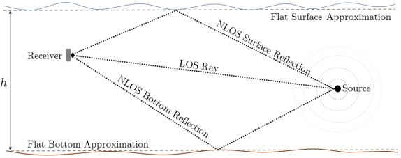
Figure 1: A 222-dimensional illustration of the three-ray model. When the surface and bottom are approximately flat in the operational area [33, 34], this model enables NLOS-based localization in the potential absence of the LOS signal component, e.g., due to an occluder.

The rest of the paper is organized as follows. The remainder of this section is devoted to an outline of our notation. In Section II we formulate the problem for the three-ray signal model depicted in Fig. 1, and the MFP solution of this model is presented in Section III. The main results, including our proposed SBL method, are presented in Section IV. In Section V we derive the respective CRLB, and present empirical simulation results that corroborate our analytical derivation in Section VI. Concluding remarks are provided in Section VIII.

I-C Notation

We use x𝑥x, 𝒙𝒙x, and 𝑿𝑿X for a scalar, column vector and matrix, respectively. The superscripts ()TsuperscriptT(\cdot)^{\mathrm{T}}, ()superscript(\cdot)^{*}, ()HsuperscriptH(\cdot)^{\mathrm{H}}, and ()1superscript1(\cdot)^{-1} denote the transposition, complex conjugation, conjugate transposition, and inverse operators, respectively. We use 𝑰Ksubscript𝑰𝐾{\mbox{\boldmath$I$}}_{K} to denote the K×K𝐾𝐾K\times K identity matrix, and 𝐎𝐎\mathbf{O} for the all-zeros matrix. The pinning vector 𝒆ksubscript𝒆𝑘{\mbox{\boldmath$e$}}_{k} denotes the k𝑘k-th column of the identity matrix, with context-dependent dimension. Further, δk𝒆kT𝒆subscript𝛿𝑘superscriptsubscript𝒆𝑘Tsubscript𝒆\delta_{k\ell}\triangleq{\mbox{\boldmath$e$}}_{k}^{\mathrm{T}}{\mbox{\boldmath$e$}}_{\ell} denotes the Kronecker delta of k𝑘k and \ell. 𝔼[]𝔼delimited-[]\mathbb{E}[\cdot] denotes expectation, λmax()subscript𝜆\lambda_{\max}\left(\cdot\right) denotes the largest eigenvalue of its (square) matrix argument, and the Diag()Diag\operatorname{Diag}(\cdot) operator forms an M×M𝑀𝑀M\times M diagonal matrix from its M𝑀M-dimensional vector argument. The Kronecker product is denoted by tensor-product\otimes. We use ȷitalic-ȷ\jmath (a dotless j𝑗j) to denote 11\sqrt{-1}; {}\Re\{\cdot\} and {}\Im\{\cdot\} denote the real and imaginary parts (respectively) of their complex-valued arguments. The 2superscript2\ell^{2} norm is denoted by 2subscriptdelimited-∥∥2\left\lVert\cdot\right\rVert_{2}, and rank()rank\operatorname{rank}(\cdot) denotes the rank of its matrix argument. The symbols \mathbb{R} and \mathbb{C} denote the real line and complex plane, respectively. We use ¯¯\overline{\hbox{}}𝒙𝒙x to denote the (normalized) discrete Fourier transform (DFT) of 𝒙𝒙x, and 𝒙^^𝒙\widehat{{\mbox{\boldmath$x$}}} to denote an estimate thereof. We use 𝒪()𝒪\mathcal{O}(\cdot) to denote the standard big O notation [35].

II Problem Formulation

Consider L𝐿L spatially-diverse, time-synchronized receivers at known locations, each consisting of a single omni-directional hydrophone.444We focus on the single sensor case for convenience. However, our methodology can in principle be used when the receivers have sensor arrays. Furthermore, consider the presence of an unknown signal in an isotropic homogeneous medium, emitted from a source whose deterministic, unknown position is denoted by the vector of coordinates 𝒑3×1𝒑superscript31{\mbox{\boldmath$p$}}\in\mathbb{R}^{3\times 1}. We assume that the source is static, and is located sufficiently far from all L𝐿L receivers to permit a planar wavefront (far-field) approximation in the shallow-water waveguide. Each receiver records the measured acoustic signal on a fixed observation time interval, which after sampling and baseband conversion amounts to N𝑁N samples. We further assume that the area of operation can be considered as a shallow-water environment, and that the ocean floor depth in the relevant area of operation555The smallest rectangular area encompassing the source and receivers. is approximately constant [36]. We restrict our scope to (approximately) isovelocity environments and high frequency signals, in which the straight-ray model approximately holds. Since we focus on short ranges in shallow-water environments, we neglect nonlinear propagation effects in the waveguide.

Although the underwater acoustic channel generally gives rise to an equivalent rich multipath channel, a relatively simple, yet useful, approach is the three-ray model, illustrated in Fig. 1. In this approach, the modeled signal components are:

  1. 1.

    The direct-path LOS component;

  2. 2.

    The surface reflection NLOS component; and

  3. 3.

    The bottom reflection NLOS component.

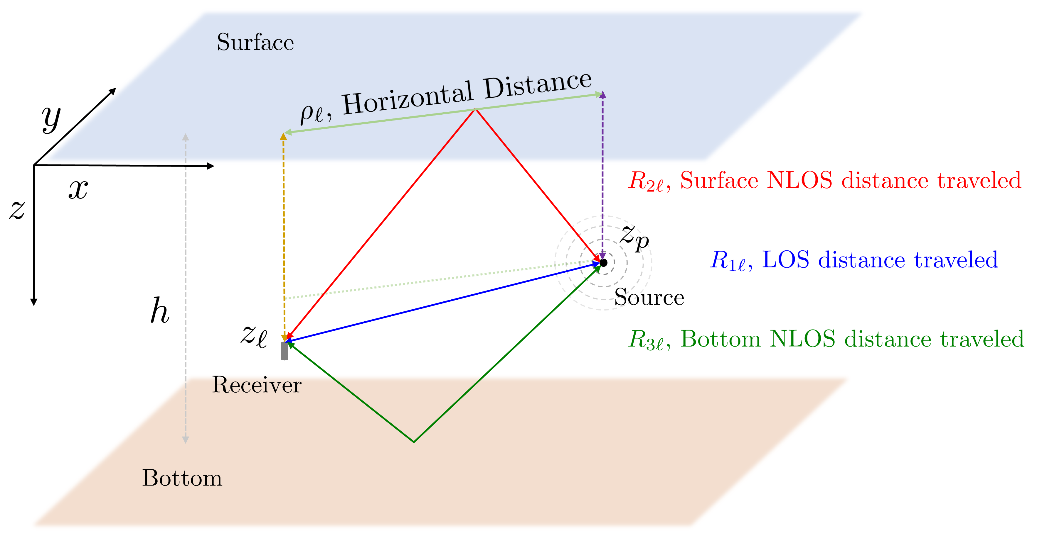
Accordingly, the associated distances traveled by these components from the source to the \ell-th receiver are given by [37]

R1subscript𝑅1\displaystyle R_{1\ell} 𝒑𝒑2, (LOS)absentsubscriptnormsubscript𝒑𝒑2 (LOS)\displaystyle\triangleq\|{\mbox{\boldmath$p$}}_{\ell}-{\mbox{\boldmath$p$}}\|_{2},\text{ \quad\quad\quad\quad\quad\quad\; (LOS)} (1)
R2subscript𝑅2\displaystyle R_{2\ell} ρ2+(zp+z)2, (NLOS surface)absentsuperscriptsubscript𝜌2superscriptsubscript𝑧𝑝subscript𝑧2 (NLOS surface)\displaystyle\triangleq\sqrt{\rho_{\ell}^{2}+(z_{p}+z_{\ell})^{2}},\text{ \quad\quad\;\;\;\, (NLOS surface)} (2)
R3subscript𝑅3\displaystyle R_{3\ell} ρ2+(2hzpz)2, (NLOS bottom)absentsuperscriptsubscript𝜌2superscript2subscript𝑧𝑝subscript𝑧2 (NLOS bottom)\displaystyle\triangleq\sqrt{\rho_{\ell}^{2}+(2h-z_{p}-z_{\ell})^{2}},\text{ \quad(NLOS bottom)} (3)

where 𝒑[xpypzp]T𝒑superscriptdelimited-[]subscript𝑥𝑝subscript𝑦𝑝subscript𝑧𝑝T{\mbox{\boldmath$p$}}\triangleq[x_{p}\;y_{p}\;z_{p}]^{\mathrm{T}}; 𝒑[xyz]Tsubscript𝒑superscriptdelimited-[]subscript𝑥subscript𝑦subscript𝑧T{\mbox{\boldmath$p$}}_{\ell}\triangleq[x_{\ell}\;y_{\ell}\;z_{\ell}]^{\mathrm{T}} is the position of the \ell-th receiver; ρ(xpx)2+(ypy)2subscript𝜌superscriptsubscript𝑥𝑝subscript𝑥2superscriptsubscript𝑦𝑝subscript𝑦2\rho_{\ell}\triangleq\sqrt{(x_{p}-x_{\ell})^{2}+(y_{p}-y_{\ell})^{2}} is the horizontal distance between the source and the \ell-th receiver; and hh is the bottom depth in the area of interest. An illustration of the geometry associated with (1)–(3) in our coordinate system is given in Fig. 2. Therefore, assuming isovelocity, the associated time-delays of these components are

τr(𝒑)Rrc,r{1,2,3},{1,,L},formulae-sequencesubscript𝜏𝑟𝒑subscript𝑅𝑟𝑐formulae-sequence𝑟123for-all1𝐿\tau_{r\ell}({\mbox{\boldmath$p$}})\triangleq\frac{R_{r\ell}}{c},\;r\in\{1,2,3\},\;\forall\ell\in\{1,\ldots,L\}, (4)

where c𝑐c denotes the speed of sound, assumed to be known.

This model can be viewed as a third-order approximation (with respect to the delayed signal components) of the equivalent impulse response of an acoustic channel, whose energy is concentrated in the three arrivals corresponding to the LOS component, and the surface and bottom reflections. While some unpredictable factors can give rise to additional components in the induced impulse response, the surface and bottom of the ocean are always present. Therefore, it is reasonable to incorporate these additional signal components into the model. Moreover, this simplified model allows for successful localization in the absence of (even all) LOS components in the received signals, a situation that may occur, e.g., due to the presence of potential occluders. This will be demonstrated via simulations and experiments with real data in Section VI.
Refer to caption
Figure 2: A 3-dimensional illustration of the geometry leading to (1)–(3).

II-A Baseband Signal Model

Formally, and assuming the source has been detected in a given frequency band, the sampled, baseband-converted signal from the \ell-th receiver is given by

x[n]=r=13brsr[n]+v[n]𝒔T[n]𝒃+v[n],n{1,,N},{1,,L},formulae-sequencesubscript𝑥delimited-[]𝑛superscriptsubscript𝑟13subscript𝑏𝑟subscript𝑠𝑟delimited-[]𝑛subscript𝑣delimited-[]𝑛superscriptsubscript𝒔Tdelimited-[]𝑛subscript𝒃subscript𝑣delimited-[]𝑛formulae-sequencefor-all𝑛1𝑁for-all1𝐿\begin{gathered}x_{\ell}[n]=\sum_{r=1}^{3}b_{r\ell}s_{r\ell}[n]+v_{\ell}[n]\triangleq{\mbox{\boldmath$s$}}_{\ell}^{\mathrm{T}}[n]{\mbox{\boldmath$b$}}_{\ell}+v_{\ell}[n]\in\mathbb{C},\\ \forall n\in\{1,\ldots,N\},\;\forall\ell\in\{1,\ldots,L\},\end{gathered} (5)

where we have defined 𝒔[n]=[s1[n]s2[n]s3[n]]T3×1,𝒃=[b1b2b3]T3×1formulae-sequencesubscript𝒔delimited-[]𝑛superscriptdelimited-[]subscript𝑠1delimited-[]𝑛subscript𝑠2delimited-[]𝑛subscript𝑠3delimited-[]𝑛Tsuperscript31subscript𝒃superscriptdelimited-[]subscript𝑏1subscript𝑏2subscript𝑏3Tsuperscript31{\mbox{\boldmath$s$}}_{\ell}[n]=[s_{1\ell}[n]\;s_{2\ell}[n]\;s_{3\ell}[n]]^{\mathrm{T}}\in\mathbb{C}^{3\times 1},{\mbox{\boldmath$b$}}_{\ell}=[b_{1\ell}\;b_{2\ell}\;b_{3\ell}]^{\mathrm{T}}\in\mathbb{C}^{3\times 1}, and where

  1. 1.

    brsubscript𝑏𝑟b_{r\ell}\in\mathbb{C} denotes the unknown attenuation coefficient from the source to the \ell-th sensor associated with the r𝑟r-th component (LOS or surface/bottom NLOS reflection);

  2. 2.

    sr[n]s(tτr(𝒑))|t=nTssubscript𝑠𝑟delimited-[]𝑛evaluated-at𝑠𝑡subscript𝜏𝑟𝒑𝑡𝑛subscript𝑇𝑠s_{r\ell}[n]\triangleq\left.s\left(t-\tau_{r\ell}({\mbox{\boldmath$p$}})\right)\right|_{t=nT_{s}}\in\mathbb{C} denotes the sampled r𝑟r-th component of the unknown signal waveform at the \ell-th sensor, where s(tτr(𝒑))𝑠𝑡subscript𝜏𝑟𝒑s\left(t-\tau_{r\ell}({\mbox{\boldmath$p$}})\right) is the analog, continuous-time waveform delayed by τr(𝒑)subscript𝜏𝑟𝒑\tau_{r\ell}({\mbox{\boldmath$p$}}), and Tssubscript𝑇𝑠T_{s} is the (known) sampling period; and

  3. 3.

    v[n]subscript𝑣delimited-[]𝑛v_{\ell}[n]\in\mathbb{C} denotes the additive noise at the \ell-th receiver, representing the overall contributions of internal receiver noise and ambient noise, modeled as a zero-mean random process with an unknown variance σv2superscriptsubscript𝜎subscript𝑣2\sigma_{v_{\ell}}^{2}.

II-B Equivalent Formulation in the Frequency Domain

Applying the normalized DFT to (5) yields the equivalent frequency-domain representation for all {1,,L}1𝐿\ell\in\{1,\ldots,L\},

 ¯x[k]subscript ¯xdelimited-[]𝑘\displaystyle\hbox to0.0pt{\hskip 0.35762pt\leavevmode\hbox{\set@color$\overline{\hbox{}}$}\hss}{\leavevmode\hbox{\set@color$x$}}_{\ell}[k] =r=13brs¯[k]eȷωkτr(𝒑)+ ¯v[k]absentsuperscriptsubscript𝑟13subscript𝑏𝑟s¯delimited-[]𝑘superscript𝑒italic-ȷsubscript𝜔𝑘subscript𝜏𝑟𝒑subscript ¯vdelimited-[]𝑘\displaystyle=\sum_{r=1}^{3}b_{r\ell}\hskip 0.15625pt\hbox to0.0pt{\leavevmode\hbox{\set@color$s$}\hss}{\hskip-0.15625pt\leavevmode\hbox{\set@color$\overline{\hbox{}}$}}[k]e^{-\jmath\omega_{k}\tau_{r\ell}({\text{\boldmath$p$}})}+\hbox to0.0pt{\hskip 0.103pt\leavevmode\hbox{\set@color$\overline{\hbox{}}$}\hss}{\leavevmode\hbox{\set@color$v$}}_{\ell}[k] (6)
s¯[k]𝒅H[k]𝒃h¯[k]+ ¯v[k]=s¯[k]h¯[k]+ ¯v[k],absents¯delimited-[]𝑘subscriptsuperscriptsubscript𝒅Hdelimited-[]𝑘subscript𝒃absentsubscript¯delimited-[]𝑘subscript ¯vdelimited-[]𝑘s¯delimited-[]𝑘subscript¯delimited-[]𝑘subscript ¯vdelimited-[]𝑘\displaystyle\triangleq\hskip 0.15625pt\hbox to0.0pt{\leavevmode\hbox{\set@color$s$}\hss}{\hskip-0.15625pt\leavevmode\hbox{\set@color$\overline{\hbox{}}$}}[k]\cdot\underbrace{{\mbox{\boldmath$d$}}_{\ell}^{\mathrm{H}}[k]{\mbox{\boldmath$b$}}_{\ell}}_{\triangleq\bar{h}_{\ell}[k]}+\hbox to0.0pt{\hskip 0.103pt\leavevmode\hbox{\set@color$\overline{\hbox{}}$}\hss}{\leavevmode\hbox{\set@color$v$}}_{\ell}[k]=\hskip 0.15625pt\hbox to0.0pt{\leavevmode\hbox{\set@color$s$}\hss}{\hskip-0.15625pt\leavevmode\hbox{\set@color$\overline{\hbox{}}$}}[k]\cdot\bar{h}_{\ell}[k]+\hbox to0.0pt{\hskip 0.103pt\leavevmode\hbox{\set@color$\overline{\hbox{}}$}\hss}{\leavevmode\hbox{\set@color$v$}}_{\ell}[k]\in\mathbb{C},

where we have defined

𝒅[k]subscript𝒅delimited-[]𝑘\displaystyle{\mbox{\boldmath$d$}}_{\ell}[k] [eȷωkτ1(𝒑)eȷωkτ2(𝒑)eȷωkτ3(𝒑)]H3×1,absentsuperscriptdelimited-[]superscript𝑒italic-ȷsubscript𝜔𝑘subscript𝜏1𝒑superscript𝑒italic-ȷsubscript𝜔𝑘subscript𝜏2𝒑superscript𝑒italic-ȷsubscript𝜔𝑘subscript𝜏3𝒑Hsuperscript31\displaystyle\triangleq[e^{-\jmath\omega_{k}\tau_{1\ell}({\text{\boldmath$p$}})}\;e^{-\jmath\omega_{k}\tau_{2\ell}({\text{\boldmath$p$}})}\;e^{-\jmath\omega_{k}\tau_{3\ell}({\text{\boldmath$p$}})}]^{\mathrm{H}}\in\mathbb{C}^{3\times 1},
ωksubscript𝜔𝑘\displaystyle\omega_{k} 2π(k1)NTs+,k{1,,N}.formulae-sequenceabsent2𝜋𝑘1𝑁subscript𝑇𝑠subscriptfor-all𝑘1𝑁\displaystyle\triangleq\frac{2\pi(k-1)}{NT_{s}}\in\mathbb{R}_{+},\;\forall k\in\{1,\ldots,N\}.

For shorthand, we further define

 ¯𝒙subscript ¯𝒙\displaystyle\hbox to0.0pt{\hskip 0.35762pt\leavevmode\hbox{\set@color$\overline{\hbox{}}$}\hss}{\leavevmode\hbox{\set@color${\mbox{\boldmath$x$}}$}}_{\ell} [ ¯x[1] ¯x[N]]TN×1, ¯𝑿Diag( ¯𝒙),formulae-sequenceabsentsuperscriptdelimited-[]subscript ¯xdelimited-[]1subscript ¯xdelimited-[]𝑁Tsuperscript𝑁1subscript ¯𝑿Diagsubscript ¯𝒙\displaystyle\triangleq\left[\hbox to0.0pt{\hskip 0.35762pt\leavevmode\hbox{\set@color$\overline{\hbox{}}$}\hss}{\leavevmode\hbox{\set@color$x$}}_{\ell}[1]\cdots\hbox to0.0pt{\hskip 0.35762pt\leavevmode\hbox{\set@color$\overline{\hbox{}}$}\hss}{\leavevmode\hbox{\set@color$x$}}_{\ell}[N]\right]^{\mathrm{T}}\in\mathbb{C}^{N\times 1},{\hbox to0.0pt{\hskip 2.0347pt\leavevmode\hbox{\set@color$\overline{\hbox{}}$}\hss}{\leavevmode\hbox{\set@color${\mbox{\boldmath$X$}}$}}_{\ell}}\triangleq\operatorname{Diag}(\hbox to0.0pt{\hskip 0.35762pt\leavevmode\hbox{\set@color$\overline{\hbox{}}$}\hss}{\leavevmode\hbox{\set@color${\mbox{\boldmath$x$}}$}}_{\ell}), (7)
𝒔𝒔s¯¯\overline{\hbox{}} [s¯[1]s¯[N]]TN×1, ¯𝑺Diag(𝒔¯),formulae-sequenceabsentsuperscriptdelimited-[]s¯delimited-[]1s¯delimited-[]𝑁Tsuperscript𝑁1 ¯𝑺Diag𝒔¯\displaystyle\triangleq\left[\hskip 0.15625pt\hbox to0.0pt{\leavevmode\hbox{\set@color$s$}\hss}{\hskip-0.15625pt\leavevmode\hbox{\set@color$\overline{\hbox{}}$}}[1]\cdots\hskip 0.15625pt\hbox to0.0pt{\leavevmode\hbox{\set@color$s$}\hss}{\hskip-0.15625pt\leavevmode\hbox{\set@color$\overline{\hbox{}}$}}[N]\right]^{\mathrm{T}}\in\mathbb{C}^{N\times 1},\quad\;\hbox to0.0pt{\hskip 0.85414pt\leavevmode\hbox{\set@color$\overline{\hbox{}}$}\hss}{\leavevmode\hbox{\set@color${\mbox{\boldmath$S$}}$}}\triangleq\operatorname{Diag}(\hskip 0.15625pt\hbox to0.0pt{\leavevmode\hbox{\set@color${\mbox{\boldmath$s$}}$}\hss}{\hskip-0.15625pt\leavevmode\hbox{\set@color$\overline{\hbox{}}$}}),
 ¯𝒗subscript ¯𝒗\displaystyle\hbox to0.0pt{\hskip 0.103pt\leavevmode\hbox{\set@color$\overline{\hbox{}}$}\hss}{\leavevmode\hbox{\set@color${\mbox{\boldmath$v$}}$}}_{\ell} [ ¯v[1] ¯v[N]]TN×1,absentsuperscriptdelimited-[]subscript ¯vdelimited-[]1subscript ¯vdelimited-[]𝑁Tsuperscript𝑁1\displaystyle\triangleq\left[\hbox to0.0pt{\hskip 0.103pt\leavevmode\hbox{\set@color$\overline{\hbox{}}$}\hss}{\leavevmode\hbox{\set@color$v$}}_{\ell}[1]\cdots\hbox to0.0pt{\hskip 0.103pt\leavevmode\hbox{\set@color$\overline{\hbox{}}$}\hss}{\leavevmode\hbox{\set@color$v$}}_{\ell}[N]\right]^{\mathrm{T}}\in\mathbb{C}^{N\times 1},
𝑫subscript𝑫\displaystyle{\mbox{\boldmath$D$}}_{\ell} [𝒅[1]𝒅[N]]TN×3,𝑯Diag(𝑫𝒃).formulae-sequenceabsentsuperscriptdelimited-[]subscript𝒅delimited-[]1subscript𝒅delimited-[]𝑁Tsuperscript𝑁3subscript𝑯Diagsubscript𝑫subscript𝒃\displaystyle\triangleq\left[{\mbox{\boldmath$d$}}_{\ell}[1]\cdots{\mbox{\boldmath$d$}}_{\ell}[N]\right]^{\mathrm{T}}\in\mathbb{C}^{N\times 3},{\mbox{\boldmath$H$}}_{\ell}\triangleq\operatorname{Diag}\left({\mbox{\boldmath$D$}}_{\ell}{\mbox{\boldmath$b$}}_{\ell}\right).

Note that 𝑫subscript𝑫{\mbox{\boldmath$D$}}_{\ell} and 𝑯subscript𝑯{\mbox{\boldmath$H$}}_{\ell} are nonlinear functions of the unknown emitter position 𝒑𝒑p, as suggested by the definition of 𝒅[k]subscript𝒅delimited-[]𝑘{\mbox{\boldmath$d$}}_{\ell}[k] above and (1)–(4), though we omit this for brevity. With this notation, we may now write (6) compactly as

 ¯𝒙=𝑯𝒔¯+ ¯𝒗N×1,{1,,L}.formulae-sequencesubscript ¯𝒙subscript𝑯𝒔¯subscript ¯𝒗superscript𝑁1for-all1𝐿\hbox to0.0pt{\hskip 0.35762pt\leavevmode\hbox{\set@color$\overline{\hbox{}}$}\hss}{\leavevmode\hbox{\set@color${\mbox{\boldmath$x$}}$}}_{\ell}={\mbox{\boldmath$H$}}_{\ell}\hskip 0.15625pt\hbox to0.0pt{\leavevmode\hbox{\set@color${\mbox{\boldmath$s$}}$}\hss}{\hskip-0.15625pt\leavevmode\hbox{\set@color$\overline{\hbox{}}$}}+\hbox to0.0pt{\hskip 0.103pt\leavevmode\hbox{\set@color$\overline{\hbox{}}$}\hss}{\leavevmode\hbox{\set@color${\mbox{\boldmath$v$}}$}}_{\ell}\in\mathbb{C}^{N\times 1},\;\forall\ell\in\{1,\ldots,L\}. (8)

Thus, the localization problem can be formulated as follows: Problem: Given the measurements { ¯𝐱N×1}=1Lsuperscriptsubscriptsubscript ¯𝐱superscript𝑁11𝐿\left\{\hbox to0.0pt{\hskip 0.35762pt\leavevmode\hbox{\set@color$\overline{\hbox{}}$}\hss}{\leavevmode\hbox{\set@color${\mbox{\boldmath$x$}}$}}_{\ell}\in\mathbb{C}^{N\times 1}\right\}_{\ell=1}^{L} of the signal model (8), localize the source, namely estimate 𝐩𝐩p. We emphasize that although we are interested solely in 𝒑𝒑p, the channel parameters {𝒃}subscript𝒃\{{\mbox{\boldmath$b$}}_{\ell}\} and the DFT coefficients 𝒔𝒔s¯¯\overline{\hbox{}} of the emitted waveform are unknown as well.

III The Matched Field Processing Solution

The key assumption of MFP approaches is that, for a given hypothesized emitter location 𝒑𝒑p, the channel response 𝑯subscript𝑯{\mbox{\boldmath$H$}}_{\ell} is fully predictable.666Otherwise, infeasible high-dimensional optimization is required. For the model (5), the attenuation coefficients {𝒃}subscript𝒃\{{\mbox{\boldmath$b$}}_{\ell}\} can be assumed to be given by777Ignoring the effects of volume absorption in water, which are minimal.

b1subscript𝑏1\displaystyle b_{1\ell} =1R1, (LOS attenuation)absent1subscript𝑅1 (LOS attenuation)\displaystyle=\frac{1}{R_{1\ell}},\text{ \quad(LOS attenuation)} (9)
b2subscript𝑏2\displaystyle b_{2\ell} =1R2, (NLOS surface reflection attenuation)absent1subscript𝑅2 (NLOS surface reflection attenuation)\displaystyle=\frac{-1}{R_{2\ell}},\text{ \quad(NLOS surface reflection attenuation)} (10)
b3subscript𝑏3\displaystyle b_{3\ell} =κbR3, (NLOS bottom reflection attenuation)absentsubscript𝜅𝑏subscript𝑅3 (NLOS bottom reflection attenuation)\displaystyle=\frac{\kappa_{b}}{R_{3\ell}},\text{ \quad(NLOS bottom reflection attenuation)} (11)

for all {1,,L}1𝐿\ell\in\{1,\ldots,L\}, where κbsubscript𝜅𝑏\kappa_{b} is the bottom reflection coefficient, which (presumably) can be determined based on prior physical knowledge (e.g., assuming the bottom is sand, silt, clay, rock, etc.) and the angle of incidence, and is assumed to be known within the MFP framework for a given hypothesized emitter location 𝒑𝒑p. For (10), we assumed a perfectly reflecting ocean surface [8, 38], which approximately holds for calm shallow waters. Based on this knowledge, the channel responses {𝑯}subscript𝑯\{{\mbox{\boldmath$H$}}_{\ell}\} can be readily computed.

The MFP solution for the three-ray model, denoted for convenience as MFP3, is then given by

𝒑^MFP3argmin𝒑3×1min𝒔¯N×1C~MFP3(𝒑,𝒔¯),subscript^𝒑MFP3𝒑superscript31argminsubscriptbold-¯𝒔superscript𝑁1subscript~𝐶MFP3𝒑𝒔¯\widehat{{\mbox{\boldmath$p$}}}_{\text{\tiny MFP3}}\triangleq\underset{\text{\boldmath$p$}\in\mathbb{R}^{3\times 1}}{\operatorname*{argmin}}\;\min_{\text{\boldmath$\bar{s}$}\in\mathbb{C}^{N\times 1}}\widetilde{C}_{\text{\tiny MFP3}}({\mbox{\boldmath$p$}},\hskip 0.15625pt\hbox to0.0pt{\leavevmode\hbox{\set@color${\mbox{\boldmath$s$}}$}\hss}{\hskip-0.15625pt\leavevmode\hbox{\set@color$\overline{\hbox{}}$}}), (12)

where

C~MFP3(𝒑,𝒔¯)=1L ¯𝒙𝑯(𝒑)𝒔¯22,subscript~𝐶MFP3𝒑𝒔¯superscriptsubscript1𝐿superscriptsubscriptdelimited-∥∥subscript ¯𝒙subscript𝑯𝒑𝒔¯22\widetilde{C}_{\text{\tiny MFP3}}({\mbox{\boldmath$p$}},\hskip 0.15625pt\hbox to0.0pt{\leavevmode\hbox{\set@color${\mbox{\boldmath$s$}}$}\hss}{\hskip-0.15625pt\leavevmode\hbox{\set@color$\overline{\hbox{}}$}})\triangleq\sum_{\ell=1}^{L}\left\lVert\hbox to0.0pt{\hskip 0.35762pt\leavevmode\hbox{\set@color$\overline{\hbox{}}$}\hss}{\leavevmode\hbox{\set@color${\mbox{\boldmath$x$}}$}}_{\ell}-{\mbox{\boldmath$H$}}_{\ell}({\mbox{\boldmath$p$}})\hskip 0.15625pt\hbox to0.0pt{\leavevmode\hbox{\set@color${\mbox{\boldmath$s$}}$}\hss}{\hskip-0.15625pt\leavevmode\hbox{\set@color$\overline{\hbox{}}$}}\right\rVert_{2}^{2}, (13)

and here we write 𝑯(𝒑)subscript𝑯𝒑{\mbox{\boldmath$H$}}_{\ell}({\mbox{\boldmath$p$}}) (rather than 𝑯subscript𝑯{\mbox{\boldmath$H$}}_{\ell}) to emphasize the dependence on 𝒑𝒑p. The simplified MFP3 solution is given by

𝒑^MFP3=argmax𝒑3×1k=1N| ¯𝒙[k]H ¯𝒉k(𝒑)|2 ¯𝒉k(𝒑)2,subscript^𝒑MFP3𝒑superscript31argmaxsuperscriptsubscript𝑘1𝑁superscript ¯𝒙superscriptdelimited-[]𝑘Hsubscript ¯𝒉𝑘𝒑2superscriptnormsubscript ¯𝒉𝑘𝒑2\widehat{{\mbox{\boldmath$p$}}}_{\text{\tiny MFP3}}=\underset{\text{\boldmath$p$}\in\mathbb{R}^{3\times 1}}{\operatorname*{argmax}}\;\sum_{k=1}^{N}\frac{\left|\hbox to0.0pt{\hskip 0.35762pt\leavevmode\hbox{\set@color$\overline{\hbox{}}$}\hss}{\leavevmode\hbox{\set@color${\mbox{\boldmath$x$}}$}}[k]^{\mathrm{H}}\hbox to0.0pt{\hskip 0.38078pt\leavevmode\hbox{\set@color$\overline{\hbox{}}$}\hss}{\leavevmode\hbox{\set@color${\mbox{\boldmath$h$}}$}}_{k}({\mbox{\boldmath$p$}})\right|^{2}}{\|\hbox to0.0pt{\hskip 0.38078pt\leavevmode\hbox{\set@color$\overline{\hbox{}}$}\hss}{\leavevmode\hbox{\set@color${\mbox{\boldmath$h$}}$}}_{k}({\mbox{\boldmath$p$}})\|^{2}}, (14)

where we have defined, for every k𝑘k-th DFT component,

 ¯𝒙[k] ¯𝒙delimited-[]𝑘\displaystyle\hbox to0.0pt{\hskip 0.35762pt\leavevmode\hbox{\set@color$\overline{\hbox{}}$}\hss}{\leavevmode\hbox{\set@color${\mbox{\boldmath$x$}}$}}[k] [x¯1[k]x¯L[k]]TL×1,absentsuperscriptdelimited-[]subscript¯𝑥1delimited-[]𝑘subscript¯𝑥𝐿delimited-[]𝑘Tsuperscript𝐿1\displaystyle\triangleq\left[\bar{x}_{1}[k]\,\cdots\,\bar{x}_{L}[k]\right]^{\mathrm{T}}\in\mathbb{C}^{L\times 1},
 ¯𝒉k(𝒑)subscript ¯𝒉𝑘𝒑\displaystyle\hbox to0.0pt{\hskip 0.38078pt\leavevmode\hbox{\set@color$\overline{\hbox{}}$}\hss}{\leavevmode\hbox{\set@color${\mbox{\boldmath$h$}}$}}_{k}({\mbox{\boldmath$p$}}) [h¯1[k]h¯L[k]]TL×1,absentsuperscriptdelimited-[]subscript¯1delimited-[]𝑘subscript¯𝐿delimited-[]𝑘Tsuperscript𝐿1\displaystyle\triangleq\left[\bar{h}_{1}[k]\;\cdots\;\bar{h}_{L}[k]\right]^{\mathrm{T}}\in\mathbb{C}^{L\times 1},

using  ¯𝒉k(𝒑)subscript ¯𝒉𝑘𝒑\hbox to0.0pt{\hskip 0.38078pt\leavevmode\hbox{\set@color$\overline{\hbox{}}$}\hss}{\leavevmode\hbox{\set@color${\mbox{\boldmath$h$}}$}}_{k}({\mbox{\boldmath$p$}}) (rather than  ¯𝒉ksubscript ¯𝒉𝑘\hbox to0.0pt{\hskip 0.38078pt\leavevmode\hbox{\set@color$\overline{\hbox{}}$}\hss}{\leavevmode\hbox{\set@color${\mbox{\boldmath$h$}}$}}_{k}) to emphasize the dependence on 𝒑𝒑p. For completeness of the exposition, the derivation of the simplified form (14) is given in the supplementary materials.

In (14), the channel impulse response  ¯𝒉k(𝒑)subscript ¯𝒉𝑘𝒑\hbox to0.0pt{\hskip 0.38078pt\leavevmode\hbox{\set@color$\overline{\hbox{}}$}\hss}{\leavevmode\hbox{\set@color${\mbox{\boldmath$h$}}$}}_{k}({\mbox{\boldmath$p$}}) is considered to be fully known for any given hypothesized position 𝒑𝒑p (via (1)–(4) and (9)–(11)). In other words, assuming perfect knowledge of 𝒃1,,𝒃Lsubscript𝒃1subscript𝒃𝐿{\mbox{\boldmath$b$}}_{1},\ldots,{\mbox{\boldmath$b$}}_{L} means that any relevant physical parameter, such as the ocean bottom sediment coefficient κbsubscript𝜅𝑏\kappa_{b} in (11), is assumed to be perfectly known as well. We relax this (somewhat unrealistic) assumption in our semi-blind localization approach described next.

IV The Proposed Semi-Blind Localization Method

As our semi-blind framework, we only assume that the bottom depth hh is known, but we do not assume that we have any prior knowledge of the channel attenuation coefficients. Thus, since the waveform emitted from the source is also unknown, we may assume without loss of generality (w.l.o.g.) that 𝒔¯2=1subscriptnorm𝒔¯21\|\hskip 0.15625pt\hbox to0.0pt{\leavevmode\hbox{\set@color${\mbox{\boldmath$s$}}$}\hss}{\hskip-0.15625pt\leavevmode\hbox{\set@color$\overline{\hbox{}}$}}\|_{2}=1, viz., 𝒔¯𝒮N{𝒛N×1:𝒛2=1}𝒔¯subscript𝒮𝑁conditional-set𝒛superscript𝑁1subscriptnorm𝒛21\hskip 0.15625pt\hbox to0.0pt{\leavevmode\hbox{\set@color${\mbox{\boldmath$s$}}$}\hss}{\hskip-0.15625pt\leavevmode\hbox{\set@color$\overline{\hbox{}}$}}\in\mathcal{S}_{N}\triangleq\{{\mbox{\boldmath$z$}}\in\mathbb{C}^{N\times 1}\colon\|{\mbox{\boldmath$z$}}\|_{2}=1\}, where 𝒮Nsubscript𝒮𝑁\mathcal{S}_{N} is the N𝑁N-dimensional unit sphere. This assumption, which is common in similar (semi-)blind formulations (e.g., [39]), is justified due to the inherent scaling ambiguity in (8),

α:𝑯𝒔¯:𝛼subscript𝑯𝒔¯\displaystyle\alpha\in\mathbb{C}:{\mbox{\boldmath$H$}}_{\ell}\hskip 0.15625pt\hbox to0.0pt{\leavevmode\hbox{\set@color${\mbox{\boldmath$s$}}$}\hss}{\hskip-0.15625pt\leavevmode\hbox{\set@color$\overline{\hbox{}}$}} =Diag(𝑫𝒃)𝒔¯=Diag(𝑫(1α𝒃𝒃~))(α𝒔¯𝒔¯~)absentDiagsubscript𝑫subscript𝒃𝒔¯Diagsubscript𝑫subscript1𝛼subscript𝒃absentsubscript~𝒃subscript𝛼𝒔¯absent~𝒔¯\displaystyle=\operatorname{Diag}\left({\mbox{\boldmath$D$}}_{\ell}{\mbox{\boldmath$b$}}_{\ell}\right)\hskip 0.15625pt\hbox to0.0pt{\leavevmode\hbox{\set@color${\mbox{\boldmath$s$}}$}\hss}{\hskip-0.15625pt\leavevmode\hbox{\set@color$\overline{\hbox{}}$}}=\operatorname{Diag}\Big{(}{\mbox{\boldmath$D$}}_{\ell}\big{(}\underbrace{\tfrac{1}{\alpha}{\mbox{\boldmath$b$}}_{\ell}}_{\triangleq\,\widetilde{{\mbox{\boldmath$b$}}}_{\ell}}\big{)}\Big{)}(\underbrace{\alpha\hskip 0.15625pt\hbox to0.0pt{\leavevmode\hbox{\set@color${\mbox{\boldmath$s$}}$}\hss}{\hskip-0.15625pt\leavevmode\hbox{\set@color$\overline{\hbox{}}$}}}_{\triangleq\,\widetilde{\hskip 0.85938pt\hbox to0.0pt{\leavevmode\hbox{\set@color${\mbox{\boldmath$s$}}$}\hss}{\hskip-0.85938pt\leavevmode\hbox{\set@color$\overline{\hbox{}}$}}}})
=Diag(𝑫𝒃~)𝑯~𝒔¯~=𝑯~𝒔¯~,{1,,L},formulae-sequenceabsentsubscriptDiagsubscript𝑫subscript~𝒃absentsubscript~𝑯~𝒔¯subscript~𝑯~𝒔¯for-all1𝐿\displaystyle=\underbrace{\operatorname{Diag}\left({\mbox{\boldmath$D$}}_{\ell}\widetilde{{\mbox{\boldmath$b$}}}_{\ell}\right)}_{\triangleq\,\widetilde{{\mbox{\boldmath$H$}}}_{\ell}}\widetilde{\hskip 0.15625pt\hbox to0.0pt{\leavevmode\hbox{\set@color${\mbox{\boldmath$s$}}$}\hss}{\hskip-0.15625pt\leavevmode\hbox{\set@color$\overline{\hbox{}}$}}}=\widetilde{{\mbox{\boldmath$H$}}}_{\ell}\widetilde{\hskip 0.15625pt\hbox to0.0pt{\leavevmode\hbox{\set@color${\mbox{\boldmath$s$}}$}\hss}{\hskip-0.15625pt\leavevmode\hbox{\set@color$\overline{\hbox{}}$}}},\quad\forall\ell\in\{1,\ldots,L\},

which, granted, is immaterial to our localization problem.

Our proposed SBL solution can be viewed as the MLE of 𝒑𝒑p, obtained by joint estimation of all the unknown deterministic model parameters, under the assumption that the noise processes { ¯𝒗}=1Lsuperscriptsubscriptsubscript ¯𝒗1𝐿\{\hbox to0.0pt{\hskip 0.103pt\leavevmode\hbox{\set@color$\overline{\hbox{}}$}\hss}{\leavevmode\hbox{\set@color${\mbox{\boldmath$v$}}$}}_{\ell}\}_{\ell=1}^{L} from all different sensors are temporally white complex normal (CN) processes, mutually statistically independent, with equal variances. In this case, the MLE of 𝒑𝒑p is the solution to the nonlinear least squares problem

𝒑^SBLargmin𝒑3×1min𝒔¯𝒮N𝑩3×LC~SBL(𝒑,𝒔¯,𝑩)CSBL(𝒑)argmin𝒑3×1CSBL(𝒑),subscript^𝒑SBL𝒑superscript31argminsubscriptsubscriptbold-¯𝒔subscript𝒮𝑁𝑩superscript3𝐿subscript~𝐶SBL𝒑𝒔¯𝑩subscript𝐶SBL𝒑𝒑superscript31argminsubscript𝐶SBL𝒑\widehat{{\mbox{\boldmath$p$}}}_{\text{\tiny SBL}}\triangleq\underset{\text{\boldmath$p$}\in\mathbb{R}^{3\times 1}}{\operatorname*{argmin}}\;\underbrace{\min_{\begin{subarray}{c}\text{\boldmath$\bar{s}$}\in\mathcal{S}_{N}\\ {\text{\boldmath$B$}}\in\mathbb{C}^{3\times L}\end{subarray}}\widetilde{C}_{\text{\tiny SBL}}({\mbox{\boldmath$p$}},\hskip 0.15625pt\hbox to0.0pt{\leavevmode\hbox{\set@color${\mbox{\boldmath$s$}}$}\hss}{\hskip-0.15625pt\leavevmode\hbox{\set@color$\overline{\hbox{}}$}},{\mbox{\boldmath$B$}})}_{C_{\text{\tiny SBL}}(\text{\boldmath$p$})}\triangleq\underset{\text{\boldmath$p$}\in\mathbb{R}^{3\times 1}}{\operatorname*{argmin}}\;C_{\text{\tiny SBL}}({\mbox{\boldmath$p$}}),\\ (15)

where the objective function C~SBL(𝒑,𝒔¯,𝑩)subscript~𝐶SBL𝒑𝒔¯𝑩\widetilde{C}_{\text{\tiny SBL}}({\mbox{\boldmath$p$}},\hskip 0.15625pt\hbox to0.0pt{\leavevmode\hbox{\set@color${\mbox{\boldmath$s$}}$}\hss}{\hskip-0.15625pt\leavevmode\hbox{\set@color$\overline{\hbox{}}$}},{\mbox{\boldmath$B$}}) is defined as

C~SBL(𝒑,𝒔¯,𝑩)=1L ¯𝒙Diag(𝑫(𝒑)𝒃)𝒔¯22,subscript~𝐶SBL𝒑𝒔¯𝑩superscriptsubscript1𝐿superscriptsubscriptdelimited-∥∥subscript ¯𝒙Diagsubscript𝑫𝒑subscript𝒃𝒔¯22\widetilde{C}_{\text{\tiny SBL}}({\mbox{\boldmath$p$}},\hskip 0.15625pt\hbox to0.0pt{\leavevmode\hbox{\set@color${\mbox{\boldmath$s$}}$}\hss}{\hskip-0.15625pt\leavevmode\hbox{\set@color$\overline{\hbox{}}$}},{\mbox{\boldmath$B$}})\triangleq\sum_{\ell=1}^{L}\left\lVert\hbox to0.0pt{\hskip 0.35762pt\leavevmode\hbox{\set@color$\overline{\hbox{}}$}\hss}{\leavevmode\hbox{\set@color${\mbox{\boldmath$x$}}$}}_{\ell}-\operatorname{Diag}\left({\mbox{\boldmath$D$}}_{\ell}({\mbox{\boldmath$p$}}){\mbox{\boldmath$b$}}_{\ell}\right)\hskip 0.15625pt\hbox to0.0pt{\leavevmode\hbox{\set@color${\mbox{\boldmath$s$}}$}\hss}{\hskip-0.15625pt\leavevmode\hbox{\set@color$\overline{\hbox{}}$}}\right\rVert_{2}^{2}, (16)

and here we write 𝑫(𝒑)subscript𝑫𝒑{\mbox{\boldmath$D$}}_{\ell}({\mbox{\boldmath$p$}}) (rather than 𝑫subscript𝑫{\mbox{\boldmath$D$}}_{\ell}) to emphasize the dependence on 𝒑𝒑p. In contrast to the MFP3 solution (12), our proposed solution (15) is due to joint estimation of all the unknown model parameters 𝒑,𝒔¯𝒑𝒔¯{\mbox{\boldmath$p$}},\hskip 0.15625pt\hbox to0.0pt{\leavevmode\hbox{\set@color${\mbox{\boldmath$s$}}$}\hss}{\hskip-0.15625pt\leavevmode\hbox{\set@color$\overline{\hbox{}}$}} and 𝑩[𝒃1𝒃L]3×L𝑩delimited-[]subscript𝒃1subscript𝒃𝐿superscript3𝐿{\mbox{\boldmath$B$}}\triangleq\left[{\mbox{\boldmath$b$}}_{1}\ldots{\mbox{\boldmath$b$}}_{L}\right]\in\mathbb{C}^{3\times L}, including the channel coefficients 𝑩𝑩B. Thus, in our proposed approach, we do not assume that the channel response is fully known for a given hypothesized position 𝒑𝒑p of the source.

Intuitively, this approach should lead to a more robust solution than MFP3 with respect to deviations from the channel knowledge (9)–(11), at the cost of extra computational effort. Fortunately, as we show in Section IV, by exploiting the low-dimensional structure of the data, the additional computational cost is negligible. Moreover, although (15) defines a nonlinear high-dimensional optimization problem with 3L3𝐿3L additional unknowns relative to MFP3, it boils down to a 333-dimensional optimization problem, similar to (14).

Our main result is the following localization algorithm:

The SBL Estimator: Input: { ¯𝒙}=1L,c,hsuperscriptsubscriptsubscript ¯𝒙1𝐿𝑐\left\{\hbox to0.0pt{\hskip 0.35762pt\leavevmode\hbox{\set@color$\overline{\hbox{}}$}\hss}{\leavevmode\hbox{\set@color${\mbox{\boldmath$x$}}$}}_{\ell}\right\}_{\ell=1}^{L},c,h, 333D grid of the volume of interest. Output: The SBL estimate, 𝒑^SBLsubscript^𝒑SBL\widehat{{\mbox{\boldmath$p$}}}_{\text{\tiny SBL}}. 1. For every candidate 𝒑𝒑p on the grid: 1.1. Compute the matrices {𝑫T𝑫}=1Lsuperscriptsubscriptsuperscriptsubscript𝑫Tsuperscriptsubscript𝑫1𝐿\{{\mbox{\boldmath$D$}}_{\ell}^{\mathrm{T}}{\mbox{\boldmath$D$}}_{\ell}^{*}\}_{\ell=1}^{L}; 1.2. Compute the Cholesky decompositions 𝑫T𝑫𝚪H𝚪3×3,{1,,L},formulae-sequencesuperscriptsubscript𝑫Tsubscriptsuperscript𝑫superscriptsubscript𝚪Hsubscript𝚪superscript33for-all1𝐿{\mbox{\boldmath$D$}}_{\ell}^{\mathrm{T}}{\mbox{\boldmath$D$}}^{*}_{\ell}\triangleq{\mbox{\boldmath$\Gamma$}}_{\ell}^{\mathrm{H}}{\mbox{\boldmath$\Gamma$}}_{\ell}\in\mathbb{C}^{3\times 3},\;\forall\ell\in\{1,\ldots,L\}, (17) and obtain the matrices {𝚪}=1Lsuperscriptsubscriptsubscript𝚪1𝐿\{{\mbox{\boldmath$\Gamma$}}_{\ell}\}_{\ell=1}^{L}; 1.3. Compute the matrix 𝑼(𝒑)[ ¯𝑿1𝑫1𝚪11 ¯𝑿L𝑫L𝚪L1]N×3L,𝑼𝒑delimited-[]subscript ¯𝑿1subscriptsuperscript𝑫1superscriptsubscript𝚪11subscript ¯𝑿𝐿subscriptsuperscript𝑫𝐿superscriptsubscript𝚪𝐿1superscript𝑁3𝐿{\mbox{\boldmath$U$}}({\mbox{\boldmath$p$}})\triangleq\left[\hbox to0.0pt{\hskip 2.0347pt\leavevmode\hbox{\set@color$\overline{\hbox{}}$}\hss}{\leavevmode\hbox{\set@color${\mbox{\boldmath$X$}}$}}_{1}{\mbox{\boldmath$D$}}^{*}_{1}{\mbox{\boldmath$\Gamma$}}_{1}^{-1}\cdots\;\hbox to0.0pt{\hskip 2.0347pt\leavevmode\hbox{\set@color$\overline{\hbox{}}$}\hss}{\leavevmode\hbox{\set@color${\mbox{\boldmath$X$}}$}}_{L}{\mbox{\boldmath$D$}}^{*}_{L}{\mbox{\boldmath$\Gamma$}}_{L}^{-1}\right]\in\mathbb{C}^{N\times 3L}, (18) and construct the matrix 𝑸~(𝒑)𝑼(𝒑)H𝑼(𝒑)3L×3L.~𝑸𝒑𝑼superscript𝒑H𝑼𝒑superscript3𝐿3𝐿\widetilde{{\mbox{\boldmath$Q$}}}({\mbox{\boldmath$p$}})\triangleq{\mbox{\boldmath$U$}}({\mbox{\boldmath$p$}})^{\mathrm{H}}{\mbox{\boldmath$U$}}({\mbox{\boldmath$p$}})\in\mathbb{C}^{3L\times 3L}. (19) 1.4. Compute λmax(𝑸~(𝒑))subscript𝜆~𝑸𝒑\lambda_{\max}\left(\widetilde{{\mbox{\boldmath$Q$}}}({\mbox{\boldmath$p$}})\right); 2. Find 𝒑^SBL,gridsubscript^𝒑SBLgrid\widehat{{\mbox{\boldmath$p$}}}_{\text{\tiny SBL},\text{grid}}, the maximizer point on the grid. 3. Return 𝒑^SBLsubscript^𝒑SBL\widehat{{\mbox{\boldmath$p$}}}_{\text{\tiny SBL}}, the solution of a nonlinear optimization solver (e.g., trust-region [40]) initialized by 𝒑^SBL,gridsubscript^𝒑SBLgrid\widehat{{\mbox{\boldmath$p$}}}_{\text{\tiny SBL},\text{grid}}.

We now provide the analysis, based on which the algorithm above is derived. For convenience, we define

𝑷s¯Diag(|𝒔¯|2)Ps(𝑰N+𝓔)+N×N,subscript𝑷s¯Diagsuperscript𝒔¯2subscript𝑃𝑠subscript𝑰𝑁𝓔superscriptsubscript𝑁𝑁{\mbox{\boldmath$P$}}_{\hskip 0.85938pt\hbox to0.0pt{\leavevmode\hbox{\set@color$s$}\hss}{\hskip-0.85938pt\leavevmode\hbox{\set@color$\overline{\hbox{}}$}}}\triangleq\operatorname{Diag}(|\hskip 0.15625pt\hbox to0.0pt{\leavevmode\hbox{\set@color${\mbox{\boldmath$s$}}$}\hss}{\hskip-0.15625pt\leavevmode\hbox{\set@color$\overline{\hbox{}}$}}|^{2})\triangleq P_{s}\cdot\left({\mbox{\boldmath$I$}}_{N}+{\mbox{\boldmath$\mathcal{E}$}}\right)\in\mathbb{R}_{+}^{N\times N}, (20)

where Ps+subscript𝑃𝑠subscriptP_{s}\in\mathbb{R}_{+} is the average signal power (with ||2|\cdot|^{2} operating elementwise), and 𝓔𝓔\mathcal{E} is a diagonal matrix with “small” elements, such that εmax|λmax(𝓔)|<1subscript𝜀subscript𝜆𝓔1\varepsilon_{\max}\triangleq|\lambda_{\max}\left({\mbox{\boldmath$\mathcal{E}$}}\right)|<1.

Proposition 1 (SBL for Spectrally Flat Waveforms).

Consider the case where 𝓔=𝐎𝓔𝐎{\mbox{\boldmath$\mathcal{E}$}}=\mathbf{O}, and define the data-dependent matrix,

𝑸(𝒑)=1L ¯𝐗𝑫(𝑫T𝑫)1( ¯𝐗𝑫)HN×N,𝑸𝒑superscriptsubscript1𝐿subscript ¯𝐗subscriptsuperscript𝑫superscriptsuperscriptsubscript𝑫Tsubscriptsuperscript𝑫1superscriptsubscript ¯𝐗subscriptsuperscript𝑫Hsuperscript𝑁𝑁{\mbox{\boldmath$Q$}}({\mbox{\boldmath$p$}})\triangleq\sum_{\ell=1}^{L}\hbox to0.0pt{\hskip 2.0347pt\leavevmode\hbox{\set@color$\overline{\hbox{}}$}\hss}{\leavevmode\hbox{\set@color${\mbox{\boldmath$X$}}$}}_{\ell}{\mbox{\boldmath$D$}}^{*}_{\ell}\left({\mbox{\boldmath$D$}}_{\ell}^{\mathrm{T}}{\mbox{\boldmath$D$}}^{*}_{\ell}\right)^{-1}\left(\hbox to0.0pt{\hskip 2.0347pt\leavevmode\hbox{\set@color$\overline{\hbox{}}$}\hss}{\leavevmode\hbox{\set@color${\mbox{\boldmath$X$}}$}}_{\ell}{\mbox{\boldmath$D$}}^{*}_{\ell}\right)^{\mathrm{H}}\in\mathbb{C}^{N\times N}, (21)

for any hypothesized source position 𝐩𝐩p. Then,

𝒑^SBL=argmax𝒑3×1λmax(𝑸(𝒑)).subscript^𝒑SBL𝒑superscript31argmaxsubscript𝜆𝑸𝒑\widehat{{\mbox{\boldmath$p$}}}_{\emph{\text{\tiny SBL}}}=\underset{\text{\boldmath$p$}\in\mathbb{R}^{3\times 1}}{\operatorname*{argmax}}\;\lambda_{\max}\left({\mbox{\boldmath$Q$}}({\mbox{\boldmath$p$}})\right). (22)

Proposition 1, whose proof is given in Appendix A, tells us that, for spectrally flat waveforms 𝒔𝒔s¯¯\overline{\hbox{}}, the source’s position estimator can be computed based only on λmax(𝑸(𝒑))subscript𝜆𝑸𝒑\lambda_{\max}\left({\mbox{\boldmath$Q$}}({\mbox{\boldmath$p$}})\right). Moreover, although our model has more unknowns, (22) is obtained by (only) a 333-dimensional optimization.

The next proposition, whose proof appears in Appendix B, states that the simplified form λmax(𝑸(𝒑))subscript𝜆𝑸𝒑\lambda_{\max}\left({\mbox{\boldmath$Q$}}({\mbox{\boldmath$p$}})\right) of the objective function can be a good approximation to (15) when 𝓔𝐎𝓔𝐎{\mbox{\boldmath$\mathcal{E}$}}\neq\mathbf{O}, namely for waveforms that are not spectrally flat. In turn, this implies that (22) can be used to localize a source emitting a general waveform.

Proposition 2 (SBL for General Waveforms).

Consider the case where 𝓔𝓔\mathcal{E} is not necessarily equal to 𝐎𝐎\mathbf{O}. Then,

𝒑^SBL=argmax𝒑3×1λmax(𝑸(𝒑))+𝒪(εmax).subscript^𝒑SBL𝒑superscript31argmaxsubscript𝜆𝑸𝒑𝒪subscript𝜀\widehat{{\mbox{\boldmath$p$}}}_{\emph{\text{\tiny SBL}}}=\underset{\text{\boldmath$p$}\in\mathbb{R}^{3\times 1}}{\operatorname*{argmax}}\;\lambda_{\max}\left({\mbox{\boldmath$Q$}}({\mbox{\boldmath$p$}})\right)+\mathcal{O}(\varepsilon_{\max}).

It follows that whenever εmax1much-less-thansubscript𝜀1\varepsilon_{\max}\ll 1, we have

𝒑^SBLargmax𝒑3×1λmax(𝑸(𝒑)).subscript^𝒑SBL𝒑superscript31argmaxsubscript𝜆𝑸𝒑\widehat{{\mbox{\boldmath$p$}}}_{\text{\tiny SBL}}\approx\underset{\text{\boldmath$p$}\in\mathbb{R}^{3\times 1}}{\operatorname*{argmax}}\;\lambda_{\max}\left({\mbox{\boldmath$Q$}}({\mbox{\boldmath$p$}})\right).

However, as we demonstrate via simulations and real data in Section VI, our proposed estimator exhibits good performance even for waveforms that are far from being spectrally flat. Thus, Proposition 2 implies that only λmax(𝑸(𝒑))subscript𝜆𝑸𝒑\lambda_{\max}\left({\mbox{\boldmath$Q$}}({\mbox{\boldmath$p$}})\right) is required for approximately optimal localization. In particular, it suffices to use, e.g., the power method, rather than computing the complete eigenvalue decomposition of 𝑸(𝒑)𝑸𝒑{\mbox{\boldmath$Q$}}({\mbox{\boldmath$p$}}). However, the computational complexity can be reduced even more, as implied by the following proposition, whose proof is given in Appendix C.

Proposition 3 (Efficient Computation of the SBL Objective Function).

Let 𝐐(𝐩)N×N𝐐𝐩superscript𝑁𝑁{\mbox{\boldmath$Q$}}({\mbox{\boldmath$p$}})\in\mathbb{C}^{N\times N} be defined as in (21). Then,

λmax(𝑸(𝒑))=λmax(𝑸~(𝒑)),subscript𝜆𝑸𝒑subscript𝜆~𝑸𝒑\lambda_{\max}\left({\mbox{\boldmath$Q$}}({\mbox{\boldmath$p$}})\right)=\lambda_{\max}\left(\widetilde{{\mbox{\boldmath$Q$}}}({\mbox{\boldmath$p$}})\right), (23)

and the complexity of computing (23) is (only) 𝒪(NL2)𝒪𝑁superscript𝐿2\mathcal{O}(NL^{2}).

We note that a naïve application of, e.g., the power method to 𝑸(𝒑)𝑸𝒑{\mbox{\boldmath$Q$}}({\mbox{\boldmath$p$}}) would cost 𝒪(N2)𝒪superscript𝑁2\mathcal{O}(N^{2}). This is already prohibitively expensive for reasonable sample sizes on the order of N103similar-to𝑁superscript103N\sim 10^{3}.

We emphasize that our proposed estimator implicitly optimizes over an additional 23L23𝐿2\cdot 3L unknown parameters—the channel attenuation coefficients 𝒃1,,𝒃Lsubscript𝒃1subscript𝒃𝐿{\mbox{\boldmath$b$}}_{1},\ldots,{\mbox{\boldmath$b$}}_{L}—relative to the MFP estimator of this model, while retaining the same order of computational complexity in terms of N𝑁N (sample size). As an intermediate summary, a comparison of several attributes of the proposed SBL with MFP3 is given in Table I.

MFP3 SBL Unknowns 𝒑,𝒔¯𝒑𝒔¯{\mbox{\boldmath$p$}},\hskip 0.15625pt\hbox to0.0pt{\leavevmode\hbox{\set@color${\mbox{\boldmath$s$}}$}\hss}{\hskip-0.15625pt\leavevmode\hbox{\set@color$\overline{\hbox{}}$}} 𝒑,𝒔¯,𝒃1,,𝒃L𝒑𝒔¯subscript𝒃1subscript𝒃𝐿{\mbox{\boldmath$p$}},\hskip 0.15625pt\hbox to0.0pt{\leavevmode\hbox{\set@color${\mbox{\boldmath$s$}}$}\hss}{\hskip-0.15625pt\leavevmode\hbox{\set@color$\overline{\hbox{}}$}},{\mbox{\boldmath$b$}}_{1},\ldots,{\mbox{\boldmath$b$}}_{L} Objective function k=1N|𝒙¯[k]H𝒉k(𝒑)|2𝒉k(𝒑)2superscriptsubscript𝑘1𝑁superscript𝒙¯superscriptdelimited-[]𝑘Hsubscript𝒉𝑘𝒑2superscriptnormsubscript𝒉𝑘𝒑2\sum_{k=1}^{N}\frac{\left|\hskip 0.49966pt\hbox to0.0pt{\leavevmode\hbox{\set@color${\mbox{\boldmath$x$}}$}\hss}{\hskip-0.49966pt\leavevmode\hbox{\set@color$\overline{\hbox{}}$}}[k]^{\mathrm{H}}{\mbox{\boldmath$h$}}_{k}({\mbox{\boldmath$p$}})\right|^{2}}{\|{\mbox{\boldmath$h$}}_{k}({\mbox{\boldmath$p$}})\|^{2}} λmax(𝑸~(𝒑))subscript𝜆~𝑸𝒑\lambda_{\max}\left(\widetilde{{\mbox{\boldmath$Q$}}}({\mbox{\boldmath$p$}})\right) Complexity 𝒪(NL)𝒪𝑁𝐿\mathcal{O}(NL) 𝒪(NL2)𝒪𝑁superscript𝐿2\mathcal{O}(NL^{2}) Required physical parameters h,c,κb,𝒃1,,𝒃L𝑐subscript𝜅𝑏subscript𝒃1subscript𝒃𝐿h,c,\kappa_{b},{\mbox{\boldmath$b$}}_{1},\ldots,{\mbox{\boldmath$b$}}_{L} h,c𝑐h,c

TABLE I: Comparison of the primary attributes of traditional MFP3 and the proposed estimator, SBL, for the three-ray model.

For the actual computation of the estimate 𝒑^SBLsubscript^𝒑SBL\widehat{{\mbox{\boldmath$p$}}}_{\text{\tiny SBL}}, we propose a two-phased approach. The first phase consists of a coarse grid search over the relevant volume of interest. In the second phase, a general purpose nonlinear optimization algorithm (e.g., trust-region methods [40]) is applied, where the solution from the first phase is used for initialization.

IV-A Interpretation of the SBL Solution

We now provide a useful interpretation of the closed-form expression (22) of our proposed solution, based on the derivation presented in Appendix A. We begin by explaining the first step, the estimation of 𝒃subscript𝒃{\mbox{\boldmath$b$}}_{\ell}. From (36), when ¯¯\overline{\hbox{}}𝑺𝑺S and 𝑫subscript𝑫{\mbox{\boldmath$D$}}_{\ell} (defined in (7)) are treated as known, we see that this first step can be regarded as compensation (or, rectification) of the attenuations of each of the three signal components. It is also enlightening to see this from the noiseless case, where

 ¯𝒙= ¯𝑺𝑫𝒃 ¯𝑺1 ¯𝒙per-frequencyelementwise division=𝑫𝒃per-frequency weightedsum of b1,b2,b3.subscript ¯𝒙subscript ¯𝑺𝑫subscript𝒃subscriptsuperscript ¯𝑺1subscript ¯𝒙per-frequencyelementwise divisionsubscriptsubscript𝑫subscript𝒃per-frequency weightedsum of b1,b2,b3\hbox to0.0pt{\hskip 0.35762pt\leavevmode\hbox{\set@color$\overline{\hbox{}}$}\hss}{\leavevmode\hbox{\set@color${\mbox{\boldmath$x$}}$}}_{\ell}=\hbox to0.0pt{\hskip 0.85414pt\leavevmode\hbox{\set@color$\overline{\hbox{}}$}\hss}{\leavevmode\hbox{\set@color${\mbox{\boldmath$S$}}$}}{\mbox{\boldmath$D$}}_{\ell}{\mbox{\boldmath$b$}}_{\ell}\;\Longrightarrow\underbrace{\hbox to0.0pt{\hskip 0.85414pt\leavevmode\hbox{\set@color$\overline{\hbox{}}$}\hss}{\leavevmode\hbox{\set@color${\mbox{\boldmath$S$}}$}}^{-1}\hbox to0.0pt{\hskip 0.35762pt\leavevmode\hbox{\set@color$\overline{\hbox{}}$}\hss}{\leavevmode\hbox{\set@color${\mbox{\boldmath$x$}}$}}_{\ell}}_{\begin{subarray}{c}\text{per-frequency}\\ {\text{elementwise division}}\end{subarray}}=\underbrace{{\mbox{\boldmath$D$}}_{\ell}{\mbox{\boldmath$b$}}_{\ell}}_{\begin{subarray}{c}\text{per-frequency weighted}\\ {\text{sum of $b_{1\ell},b_{2\ell},b_{3\ell}$}}\end{subarray}}. (24)

Substituting {𝒃^}subscript^𝒃\{\widehat{{\mbox{\boldmath$b$}}}_{\ell}\} (defined in (40)) into (16) yields after simplification (42)—the “𝒃subscript𝒃{\mbox{\boldmath$b$}}_{\ell}’s-rectified” objective, where the rectification is based on the intermediate estimators {𝒃^}subscript^𝒃\{\widehat{{\mbox{\boldmath$b$}}}_{\ell}\}, which still depend on the unknown ¯¯\overline{\hbox{}}𝑺𝑺S and 𝒑𝒑p at this phase.

Moving forward, we momentarily focus on a single (matrix) element of the sum (42). Rearranging this term, we see that

𝒔¯H ¯𝑿𝑫(𝑫T𝑷s¯𝑫)1( ¯𝑿𝑫)H𝒔¯=superscript𝒔¯Hsubscript ¯𝑿subscriptsuperscript𝑫superscriptsuperscriptsubscript𝑫Tsubscript𝑷s¯subscriptsuperscript𝑫1superscriptsubscript ¯𝑿subscriptsuperscript𝑫H𝒔¯absent\displaystyle\hskip 0.15625pt\hbox to0.0pt{\leavevmode\hbox{\set@color${\mbox{\boldmath$s$}}$}\hss}{\hskip-0.15625pt\leavevmode\hbox{\set@color$\overline{\hbox{}}$}}^{\mathrm{H}}\hbox to0.0pt{\hskip 2.0347pt\leavevmode\hbox{\set@color$\overline{\hbox{}}$}\hss}{\leavevmode\hbox{\set@color${\mbox{\boldmath$X$}}$}}_{\ell}{\mbox{\boldmath$D$}}^{*}_{\ell}\left({{\mbox{\boldmath$D$}}_{\ell}}^{\mathrm{T}}{\mbox{\boldmath$P$}}_{\hskip 0.85938pt\hbox to0.0pt{\leavevmode\hbox{\set@color$s$}\hss}{\hskip-0.85938pt\leavevmode\hbox{\set@color$\overline{\hbox{}}$}}}{\mbox{\boldmath$D$}}^{*}_{\ell}\right)^{-1}\left(\hbox to0.0pt{\hskip 2.0347pt\leavevmode\hbox{\set@color$\overline{\hbox{}}$}\hss}{\leavevmode\hbox{\set@color${\mbox{\boldmath$X$}}$}}_{\ell}{\mbox{\boldmath$D$}}^{*}_{\ell}\right)^{\mathrm{H}}\hskip 0.15625pt\hbox to0.0pt{\leavevmode\hbox{\set@color${\mbox{\boldmath$s$}}$}\hss}{\hskip-0.15625pt\leavevmode\hbox{\set@color$\overline{\hbox{}}$}}=
 ¯𝒙T ¯𝑺𝑫(𝑫T ¯𝑺T ¯𝑺𝑫)1𝑫T ¯𝑺T ¯𝒙.superscriptsubscript ¯𝒙Tsuperscript ¯𝑺subscriptsuperscript𝑫superscriptsuperscriptsubscript𝑫Tsuperscript ¯𝑺Tsuperscript ¯𝑺subscriptsuperscript𝑫1subscriptsuperscript𝑫Tsuperscript ¯𝑺Tsuperscriptsubscript ¯𝒙\displaystyle\hbox to0.0pt{\hskip 0.35762pt\leavevmode\hbox{\set@color$\overline{\hbox{}}$}\hss}{\leavevmode\hbox{\set@color${\mbox{\boldmath$x$}}$}}_{\ell}^{\mathrm{T}}\hbox to0.0pt{\hskip 0.85414pt\leavevmode\hbox{\set@color$\overline{\hbox{}}$}\hss}{\leavevmode\hbox{\set@color${\mbox{\boldmath$S$}}$}}^{*}{\mbox{\boldmath$D$}}^{*}_{\ell}\left({{\mbox{\boldmath$D$}}_{\ell}}^{\mathrm{T}}\hbox to0.0pt{\hskip 0.85414pt\leavevmode\hbox{\set@color$\overline{\hbox{}}$}\hss}{\leavevmode\hbox{\set@color${\mbox{\boldmath$S$}}$}}^{\mathrm{T}}\hbox to0.0pt{\hskip 0.85414pt\leavevmode\hbox{\set@color$\overline{\hbox{}}$}\hss}{\leavevmode\hbox{\set@color${\mbox{\boldmath$S$}}$}}^{*}{\mbox{\boldmath$D$}}^{*}_{\ell}\right)^{-1}{\mbox{\boldmath$D$}}^{\mathrm{T}}_{\ell}\hbox to0.0pt{\hskip 0.85414pt\leavevmode\hbox{\set@color$\overline{\hbox{}}$}\hss}{\leavevmode\hbox{\set@color${\mbox{\boldmath$S$}}$}}^{\mathrm{T}}\hbox to0.0pt{\hskip 0.35762pt\leavevmode\hbox{\set@color$\overline{\hbox{}}$}\hss}{\leavevmode\hbox{\set@color${\mbox{\boldmath$x$}}$}}_{\ell}^{*}. (25)

Again, focusing on the noiseless case to gain intuition, by substituting  ¯𝒙= ¯𝑺𝑫𝒃subscript ¯𝒙subscript ¯𝑺𝑫subscript𝒃\hbox to0.0pt{\hskip 0.35762pt\leavevmode\hbox{\set@color$\overline{\hbox{}}$}\hss}{\leavevmode\hbox{\set@color${\mbox{\boldmath$x$}}$}}_{\ell}=\hbox to0.0pt{\hskip 0.85414pt\leavevmode\hbox{\set@color$\overline{\hbox{}}$}\hss}{\leavevmode\hbox{\set@color${\mbox{\boldmath$S$}}$}}{\mbox{\boldmath$D$}}_{\ell}{\mbox{\boldmath$b$}}_{\ell}, we have

 ¯𝒙T ¯𝑺𝑫(𝑫T ¯𝑺T ¯𝑺𝑫)1𝑫T ¯𝑺T ¯𝒙=superscriptsubscript ¯𝒙Tsuperscript ¯𝑺subscriptsuperscript𝑫superscriptsuperscriptsubscript𝑫Tsuperscript ¯𝑺Tsuperscript ¯𝑺subscriptsuperscript𝑫1subscriptsuperscript𝑫Tsuperscript ¯𝑺Tsuperscriptsubscript ¯𝒙absent\displaystyle\hbox to0.0pt{\hskip 0.35762pt\leavevmode\hbox{\set@color$\overline{\hbox{}}$}\hss}{\leavevmode\hbox{\set@color${\mbox{\boldmath$x$}}$}}_{\ell}^{\mathrm{T}}\hbox to0.0pt{\hskip 0.85414pt\leavevmode\hbox{\set@color$\overline{\hbox{}}$}\hss}{\leavevmode\hbox{\set@color${\mbox{\boldmath$S$}}$}}^{*}{\mbox{\boldmath$D$}}^{*}_{\ell}\left({{\mbox{\boldmath$D$}}_{\ell}}^{\mathrm{T}}\hbox to0.0pt{\hskip 0.85414pt\leavevmode\hbox{\set@color$\overline{\hbox{}}$}\hss}{\leavevmode\hbox{\set@color${\mbox{\boldmath$S$}}$}}^{\mathrm{T}}\hbox to0.0pt{\hskip 0.85414pt\leavevmode\hbox{\set@color$\overline{\hbox{}}$}\hss}{\leavevmode\hbox{\set@color${\mbox{\boldmath$S$}}$}}^{*}{\mbox{\boldmath$D$}}^{*}_{\ell}\right)^{-1}{\mbox{\boldmath$D$}}^{\mathrm{T}}_{\ell}\hbox to0.0pt{\hskip 0.85414pt\leavevmode\hbox{\set@color$\overline{\hbox{}}$}\hss}{\leavevmode\hbox{\set@color${\mbox{\boldmath$S$}}$}}^{\mathrm{T}}\hbox to0.0pt{\hskip 0.35762pt\leavevmode\hbox{\set@color$\overline{\hbox{}}$}\hss}{\leavevmode\hbox{\set@color${\mbox{\boldmath$x$}}$}}_{\ell}^{*}=
𝒃T𝑫T ¯𝑺T ¯𝑺𝑫(𝑫T ¯𝑺T ¯𝑺𝑫)1𝑫T ¯𝑺T ¯𝑺𝑫𝒃=superscriptsubscript𝒃Tsuperscriptsubscript𝑫Tsuperscript ¯𝑺Tsuperscript ¯𝑺subscriptsuperscript𝑫superscriptsuperscriptsubscript𝑫Tsuperscript ¯𝑺Tsuperscript ¯𝑺subscriptsuperscript𝑫1subscriptsuperscript𝑫Tsuperscript ¯𝑺Tsuperscript ¯𝑺superscriptsubscript𝑫subscriptsuperscript𝒃absent\displaystyle{\mbox{\boldmath$b$}}_{\ell}^{\mathrm{T}}{\mbox{\boldmath$D$}}_{\ell}^{\mathrm{T}}\hbox to0.0pt{\hskip 0.85414pt\leavevmode\hbox{\set@color$\overline{\hbox{}}$}\hss}{\leavevmode\hbox{\set@color${\mbox{\boldmath$S$}}$}}^{\mathrm{T}}\hbox to0.0pt{\hskip 0.85414pt\leavevmode\hbox{\set@color$\overline{\hbox{}}$}\hss}{\leavevmode\hbox{\set@color${\mbox{\boldmath$S$}}$}}^{*}{\mbox{\boldmath$D$}}^{*}_{\ell}\left({{\mbox{\boldmath$D$}}_{\ell}}^{\mathrm{T}}\hbox to0.0pt{\hskip 0.85414pt\leavevmode\hbox{\set@color$\overline{\hbox{}}$}\hss}{\leavevmode\hbox{\set@color${\mbox{\boldmath$S$}}$}}^{\mathrm{T}}\hbox to0.0pt{\hskip 0.85414pt\leavevmode\hbox{\set@color$\overline{\hbox{}}$}\hss}{\leavevmode\hbox{\set@color${\mbox{\boldmath$S$}}$}}^{*}{\mbox{\boldmath$D$}}^{*}_{\ell}\right)^{-1}{\mbox{\boldmath$D$}}^{\mathrm{T}}_{\ell}\hbox to0.0pt{\hskip 0.85414pt\leavevmode\hbox{\set@color$\overline{\hbox{}}$}\hss}{\leavevmode\hbox{\set@color${\mbox{\boldmath$S$}}$}}^{\mathrm{T}}\hbox to0.0pt{\hskip 0.85414pt\leavevmode\hbox{\set@color$\overline{\hbox{}}$}\hss}{\leavevmode\hbox{\set@color${\mbox{\boldmath$S$}}$}}^{*}{\mbox{\boldmath$D$}}_{\ell}^{*}{\mbox{\boldmath$b$}}^{*}_{\ell}=
𝒃T𝑫T ¯𝑺T ¯𝑺𝑫𝒃= ¯𝑺𝑫𝒃2=k=1N|s¯[k]𝒅H[k]𝒃|22.superscriptsubscript𝒃Tsuperscriptsubscript𝑫Tsuperscript ¯𝑺Tsuperscript ¯𝑺subscriptsuperscript𝑫subscriptsuperscript𝒃superscriptnormsubscript ¯𝑺𝑫subscript𝒃2superscriptsubscript𝑘1𝑁superscriptsubscripts¯delimited-[]𝑘superscriptsubscript𝒅Hdelimited-[]𝑘subscript𝒃22\displaystyle{\mbox{\boldmath$b$}}_{\ell}^{\mathrm{T}}{\mbox{\boldmath$D$}}_{\ell}^{\mathrm{T}}\hbox to0.0pt{\hskip 0.85414pt\leavevmode\hbox{\set@color$\overline{\hbox{}}$}\hss}{\leavevmode\hbox{\set@color${\mbox{\boldmath$S$}}$}}^{\mathrm{T}}\hbox to0.0pt{\hskip 0.85414pt\leavevmode\hbox{\set@color$\overline{\hbox{}}$}\hss}{\leavevmode\hbox{\set@color${\mbox{\boldmath$S$}}$}}^{*}{\mbox{\boldmath$D$}}^{*}_{\ell}{\mbox{\boldmath$b$}}^{*}_{\ell}=\|\hbox to0.0pt{\hskip 0.85414pt\leavevmode\hbox{\set@color$\overline{\hbox{}}$}\hss}{\leavevmode\hbox{\set@color${\mbox{\boldmath$S$}}$}}{\mbox{\boldmath$D$}}_{\ell}{\mbox{\boldmath$b$}}_{\ell}\|^{2}=\sum_{k=1}^{N}\left|\hskip 0.15625pt\hbox to0.0pt{\leavevmode\hbox{\set@color$s$}\hss}{\hskip-0.15625pt\leavevmode\hbox{\set@color$\overline{\hbox{}}$}}[k]{\mbox{\boldmath$d$}}_{\ell}^{\mathrm{H}}[k]{\mbox{\boldmath$b$}}_{\ell}\right|_{2}^{2}.

Therefore, we interpret the maximization (42)—for a single receiver—as choosing the best set of parameters {𝒔¯,𝒑,𝒃}𝒔¯𝒑subscript𝒃\{\hskip 0.15625pt\hbox to0.0pt{\leavevmode\hbox{\set@color${\mbox{\boldmath$s$}}$}\hss}{\hskip-0.15625pt\leavevmode\hbox{\set@color$\overline{\hbox{}}$}},{\mbox{\boldmath$p$}},{\mbox{\boldmath$b$}}_{\ell}\}, in the sense that the total energy of the received signal from the source is maximized, under the hypothesized set of parameters.

Generalizing this intuition for a signal in noise, after substituting  ¯𝒙subscript ¯𝒙\hbox to0.0pt{\hskip 0.35762pt\leavevmode\hbox{\set@color$\overline{\hbox{}}$}\hss}{\leavevmode\hbox{\set@color${\mbox{\boldmath$x$}}$}}_{\ell} into (IV-A), for a sufficiently large N𝑁N, the signal-noise cross product terms will tend to zero by virtue of the law of large numbers, since the noise DFT coefficients are uncorrelated and zero-mean.

Lastly, we generalize the intuition above from a single receiver to multiple receivers. For this, recall that (42) is in fact a joint maximization of the total energy of all L𝐿L received signals from the same source. Therefore, it weights the L𝐿L signals from different relative locations to the source while taking into account that they all contain shifted versions of the same waveform. This is essentially the connecting link, and the advantage in processing the data jointly (rather than individually). This joint weighting is nontrivial in the general case. However, when the source is spectrally flat, i.e., 𝓔=𝐎𝓔𝐎{\mbox{\boldmath$\mathcal{E}$}}=\mathbf{O}, the optimal way (in the sense of (15)) to weight and combine the data from the receivers is to form the matrix 𝑸(𝒑)𝑸𝒑{\mbox{\boldmath$Q$}}({\mbox{\boldmath$p$}}) as in (21), and to compute its maximal eigenvalue (22). A natural interpretation of the maximal eigenvalue of a semi-positive definite matrix is the energy distributed along the dominant direction (orthogonal to all others) in the space spanned by the columns of this matrix. With this interpretation, the final form of the SBL solution given in (22) is now intuitive.

V The Cramér-Rao Lower Bound for SBL

We now analyze the localization accuracy limitations of the proposed solution in terms of the MSE,

MSE(𝒑^,𝒑)𝔼[𝒑^𝒑22].MSE^𝒑𝒑𝔼delimited-[]superscriptsubscriptdelimited-∥∥^𝒑𝒑22{\mathrm{MSE}}(\widehat{{\mbox{\boldmath$p$}}},{\mbox{\boldmath$p$}})\triangleq\mathbb{E}\left[\left\lVert\widehat{{\mbox{\boldmath$p$}}}-{\mbox{\boldmath$p$}}\right\rVert_{2}^{2}\right]. (26)

Specifically, we derive the CRLB for the special case 𝓔=𝐎𝓔𝐎{\mbox{\boldmath$\mathcal{E}$}}=\mathbf{O}. Unlike the common approach (e.g., as in [41, 42]), wherein both the unknown source signal and noise are considered to be random, in our model only the noise is considered random. Thus, for a given waveform, the bound can be used as a tool for designing the deployment of a network of receivers, so as to maximize accuracy in regions of higher importance.

Regardless of the constant spectral level (i.e., 𝓔=𝐎𝓔𝐎{\mbox{\boldmath$\mathcal{E}$}}=\mathbf{O}), in our general framework 𝒔¯𝒮N𝒔¯subscript𝒮𝑁\hskip 0.15625pt\hbox to0.0pt{\leavevmode\hbox{\set@color${\mbox{\boldmath$s$}}$}\hss}{\hskip-0.15625pt\leavevmode\hbox{\set@color$\overline{\hbox{}}$}}\in\mathcal{S}_{N} w.l.o.g., hence in this particular case Ps=1Nsubscript𝑃𝑠1𝑁P_{s}=\frac{1}{N}. Consequently, s¯[k]=1Neȷϕs[k]s¯delimited-[]𝑘1𝑁superscript𝑒italic-ȷsubscriptitalic-ϕ𝑠delimited-[]𝑘\hskip 0.15625pt\hbox to0.0pt{\leavevmode\hbox{\set@color$s$}\hss}{\hskip-0.15625pt\leavevmode\hbox{\set@color$\overline{\hbox{}}$}}[k]=\frac{1}{\sqrt{N}}e^{\jmath\phi_{s}[k]} for all k𝑘k, and the only waveform-related unknowns are the phases888Note that although there are N𝑁N elements in ϕssubscriptbold-italic-ϕ𝑠{\mbox{\boldmath$\phi$}}_{s}, there are only N1𝑁1N-1 degrees of freedom, since the (complex-valued) channel attenuation coefficients are considered unknown as well. Therefore, we assume w.l.o.g. that the first element of ϕssubscriptbold-italic-ϕ𝑠{\mbox{\boldmath$\phi$}}_{s}, considered as a reference phase, is zero. of the DFT coefficients, denoted collectively by ϕs[ϕs[2]ϕs[N]](N1)×1subscriptbold-italic-ϕ𝑠delimited-[]subscriptitalic-ϕ𝑠delimited-[]2subscriptitalic-ϕ𝑠delimited-[]𝑁superscript𝑁11{\mbox{\boldmath$\phi$}}_{s}\triangleq[\phi_{s}[2]\ldots\phi_{s}[N]{]}\in\mathbb{R}^{(N-1)\times 1}.

To facilitate the following derivation, we introduce a more compact representation of the measured signals. Specifically, let  ¯𝒙[ ¯𝒙1 ¯𝒙L]TNL×1 ¯𝒙superscriptdelimited-[]subscript ¯𝒙1subscript ¯𝒙𝐿Tsuperscript𝑁𝐿1\hbox to0.0pt{\hskip 0.35762pt\leavevmode\hbox{\set@color$\overline{\hbox{}}$}\hss}{\leavevmode\hbox{\set@color${\mbox{\boldmath$x$}}$}}\triangleq[\hbox to0.0pt{\hskip 0.35762pt\leavevmode\hbox{\set@color$\overline{\hbox{}}$}\hss}{\leavevmode\hbox{\set@color${\mbox{\boldmath$x$}}$}}_{1}\ldots\hbox to0.0pt{\hskip 0.35762pt\leavevmode\hbox{\set@color$\overline{\hbox{}}$}\hss}{\leavevmode\hbox{\set@color${\mbox{\boldmath$x$}}$}}_{L}]^{\mathrm{T}}\in\mathbb{C}^{NL\times 1}. Thus, (8) reads

 ¯𝒙=𝑯 𝒔¯+ ¯𝒗NL×1, ¯𝒙𝑯 𝒔¯ ¯𝒗superscript𝑁𝐿1\hbox to0.0pt{\hskip 0.35762pt\leavevmode\hbox{\set@color$\overline{\hbox{}}$}\hss}{\leavevmode\hbox{\set@color${\mbox{\boldmath$x$}}$}}={\mbox{\boldmath$H$}}\hskip 0.15625pt\hbox to0.0pt{\leavevmode\hbox{\set@color${\mbox{\boldmath$s$}}$}\hss}{\hskip-0.15625pt\leavevmode\hbox{\set@color$\overline{\hbox{}}$}}+\hbox to0.0pt{\hskip 0.103pt\leavevmode\hbox{\set@color$\overline{\hbox{}}$}\hss}{\leavevmode\hbox{\set@color${\mbox{\boldmath$v$}}$}}\in\mathbb{C}^{NL\times 1}, (27)

where 𝑯[𝑯1T𝑯LT]TNL×N𝑯superscriptdelimited-[]superscriptsubscript𝑯1Tsuperscriptsubscript𝑯𝐿TTsuperscript𝑁𝐿𝑁{\mbox{\boldmath$H$}}\triangleq\left[{\mbox{\boldmath$H$}}_{1}^{\mathrm{T}}\ldots{\mbox{\boldmath$H$}}_{L}^{\mathrm{T}}\right]^{\mathrm{T}}\in\mathbb{C}^{NL\times N} and  ¯𝒗[ ¯𝒗1 ¯𝒗L]T ¯𝒗superscriptdelimited-[]subscript ¯𝒗1subscript ¯𝒗𝐿T\hbox to0.0pt{\hskip 0.103pt\leavevmode\hbox{\set@color$\overline{\hbox{}}$}\hss}{\leavevmode\hbox{\set@color${\mbox{\boldmath$v$}}$}}\triangleq[\hbox to0.0pt{\hskip 0.103pt\leavevmode\hbox{\set@color$\overline{\hbox{}}$}\hss}{\leavevmode\hbox{\set@color${\mbox{\boldmath$v$}}$}}_{1}\ldots\hbox to0.0pt{\hskip 0.103pt\leavevmode\hbox{\set@color$\overline{\hbox{}}$}\hss}{\leavevmode\hbox{\set@color${\mbox{\boldmath$v$}}$}}_{L}]^{\mathrm{T}}. Denoting 𝝈v2[σv12σvL2]T+L×1superscriptsubscript𝝈𝑣2superscriptdelimited-[]subscriptsuperscript𝜎2subscript𝑣1subscriptsuperscript𝜎2subscript𝑣𝐿Tsuperscriptsubscript𝐿1{\mbox{\boldmath$\sigma$}}_{v}^{2}\triangleq[\sigma^{2}_{v_{1}}\ldots\sigma^{2}_{v_{L}}]^{\mathrm{T}}\in\mathbb{R}_{+}^{L\times 1}, it follows that

 ¯𝒙𝒞𝒩(𝑯 𝒔¯,Diag(𝝈v2)𝑰N).similar-to ¯𝒙𝒞𝒩𝑯 𝒔¯tensor-productDiagsubscriptsuperscript𝝈2𝑣subscript𝑰𝑁\hbox to0.0pt{\hskip 0.35762pt\leavevmode\hbox{\set@color$\overline{\hbox{}}$}\hss}{\leavevmode\hbox{\set@color${\mbox{\boldmath$x$}}$}}\sim\mathcal{CN}\left({\mbox{\boldmath$H$}}\hskip 0.15625pt\hbox to0.0pt{\leavevmode\hbox{\set@color${\mbox{\boldmath$s$}}$}\hss}{\hskip-0.15625pt\leavevmode\hbox{\set@color$\overline{\hbox{}}$}},\operatorname{Diag}({\mbox{\boldmath$\sigma$}}^{2}_{v})\otimes{\mbox{\boldmath$I$}}_{N}\right). (28)

It is well-known that for the CN signal model 𝒞𝒩(𝝁,𝑹)𝒞𝒩𝝁𝑹\mathcal{CN}\left({\mbox{\boldmath$\mu$}},{\mbox{\boldmath$R$}}\right), the Fisher information matrix (FIM) elements are given by999For the sake of clarity, we specifically use a different notation for the FIM’s elements, with slight abuse of notation also in (30)–(32). [43]

J[θi,θj]=Tr(𝑹1𝑹θi𝑹1𝑹θj)+2{𝝁Hθi𝑹1𝝁θj},i,j{1,,Kθ},formulae-sequence𝐽subscript𝜃𝑖subscript𝜃𝑗Trsuperscript𝑹1𝑹subscript𝜃𝑖superscript𝑹1𝑹subscript𝜃𝑗2superscript𝝁Hsubscript𝜃𝑖superscript𝑹1𝝁subscript𝜃𝑗for-all𝑖𝑗1subscript𝐾𝜃\begin{gathered}J[\theta_{i},\theta_{j}]=\operatorname{Tr}\left({\mbox{\boldmath$R$}}^{-1}\frac{\partial{\mbox{\boldmath$R$}}}{\partial\theta_{i}}{\mbox{\boldmath$R$}}^{-1}\frac{\partial{\mbox{\boldmath$R$}}}{\partial\theta_{j}}\right)+2\Re\left\{\frac{\partial{\mbox{\boldmath$\mu$}}^{\mathrm{H}}}{\partial\theta_{i}}{\mbox{\boldmath$R$}}^{-1}\frac{\partial{\mbox{\boldmath$\mu$}}}{\partial\theta_{j}}\right\},\\ \forall i,j\in\{1,\ldots,K_{\theta}\},\end{gathered}

where we have defined the vector of all the real-valued unknown deterministic parameters

𝜽[𝒑Tvec(ϕs)Tvec({𝑩})Tvec({𝑩})T𝝈v2]TKθ×1,𝜽superscriptdelimited-[]superscript𝒑Tvecsuperscriptsubscriptbold-italic-ϕ𝑠Tvecsuperscript𝑩Tvecsuperscript𝑩Tsuperscriptsubscript𝝈𝑣2Tsuperscriptsubscript𝐾𝜃1{\mbox{\boldmath$\theta$}}\triangleq\left[{\mbox{\boldmath$p$}}^{\mathrm{T}}\,\text{vec}({\mbox{\boldmath$\phi$}}_{s})^{\mathrm{T}}\,\text{vec}(\Re\{{\mbox{\boldmath$B$}}\})^{\mathrm{T}}\,\text{vec}(\Im\{{\mbox{\boldmath$B$}}\})^{\mathrm{T}}\,{\mbox{\boldmath$\sigma$}}_{v}^{2}\right]^{\mathrm{T}}\in\mathbb{R}^{K_{\theta}\times 1}, (29)

with Kθ=3+(N1)+23L+Lsubscript𝐾𝜃3𝑁123𝐿𝐿K_{\theta}=3+(N-1)+2\cdot 3L+L, and 𝑱(𝜽)𝑱𝜽{\mbox{\boldmath$J$}}({\mbox{\boldmath$\theta$}}) is the FIM.

It is readily seen from (28), that in our model the mean vector and covariance matrix are functions of distinct unknown parameters. This immediately implies that

J[σv12,σv22]𝐽superscriptsubscript𝜎subscript𝑣subscript12superscriptsubscript𝜎subscript𝑣subscript22\displaystyle J[\sigma_{v_{\ell_{1}}}^{2},\sigma_{v_{\ell_{2}}}^{2}] =Nδ12,1,2{1,,L},formulae-sequenceabsent𝑁subscript𝛿subscript1subscript2for-allsubscript1subscript21𝐿\displaystyle=N\cdot\delta_{\ell_{1}\ell_{2}},\;\forall\ell_{1},\ell_{2}\in\{1,\ldots,L\}, (30)
J[σv2,θ]𝐽superscriptsubscript𝜎subscript𝑣2𝜃\displaystyle J[\sigma_{v_{\ell}}^{2},\theta] =0,θσv2,formulae-sequenceabsent0for-all𝜃superscriptsubscript𝜎subscript𝑣2\displaystyle=0,\quad\quad\quad\;\forall\theta\neq\sigma_{v_{\ell}}^{2}, (31)

namely the FIM has a block diagonal structure. Furthermore, for the signal-related block, we have

J[θi,θj]=2{(𝑯 𝒔¯)Hθi(Diag1(𝝈v2)𝑰N)𝑯 𝒔¯θj},i,j{1,,Kθ},{1,,L}.formulae-sequence𝐽subscript𝜃𝑖subscript𝜃𝑗2superscript𝑯 𝒔¯Hsubscript𝜃𝑖tensor-productsuperscriptDiag1subscriptsuperscript𝝈2𝑣subscript𝑰𝑁𝑯 𝒔¯subscript𝜃𝑗for-all𝑖formulae-sequence𝑗1subscript𝐾𝜃for-all1𝐿\begin{gathered}J[\theta_{i},\theta_{j}]=2\Re\left\{\frac{\partial({\mbox{\boldmath$H$}}\hskip 0.15625pt\hbox to0.0pt{\leavevmode\hbox{\set@color${\mbox{\boldmath$s$}}$}\hss}{\hskip-0.15625pt\leavevmode\hbox{\set@color$\overline{\hbox{}}$}})^{\mathrm{H}}}{\partial\theta_{i}}\left(\operatorname{Diag}^{-1}({\mbox{\boldmath$\sigma$}}^{2}_{v})\otimes{\mbox{\boldmath$I$}}_{N}\right)\frac{\partial{\mbox{\boldmath$H$}}\hskip 0.15625pt\hbox to0.0pt{\leavevmode\hbox{\set@color${\mbox{\boldmath$s$}}$}\hss}{\hskip-0.15625pt\leavevmode\hbox{\set@color$\overline{\hbox{}}$}}}{\partial\theta_{j}}\right\},\\ \forall i,j\in\{1,\ldots,K_{\theta}\},\;\forall\ell\in\{1,\ldots,L\}.\end{gathered} (32)

When σv2=σv2superscriptsubscript𝜎subscript𝑣2superscriptsubscript𝜎𝑣2\sigma_{v_{\ell}}^{2}=\sigma_{v}^{2} for all \ell, it can be observed from (32) that the signal-related FIM block is inversely proportional to the noise variance. Hence, the associated signal-related CRLB block is inversely proportional to the signal-to-noise ratio (SNR).

It only remains to compute the derivatives of 𝑯𝑯H𝒔𝒔s¯¯\overline{\hbox{}} with respect to the parameters of 𝜽𝜽\theta, excluding 𝝈v2superscriptsubscript𝝈𝑣2{\mbox{\boldmath$\sigma$}}_{v}^{2}, which is merely technical. We defer the details of these calculations, as well as the final expressions of all the signal-related elements of the FIM to the supplementary materials, along with a Matlab implementation of this bound. Finally, the CRLB is given by101010𝑨𝑩succeeds-or-equals𝑨𝑩{\mbox{\boldmath$A$}}\succeq{\mbox{\boldmath$B$}} is to be interpreted to mean that 𝑨𝑩𝑨𝑩{\mbox{\boldmath$A$}}-{\mbox{\boldmath$B$}} is semi-positive definite.

𝔼[(𝜽^𝜽)(𝜽^𝜽)T]𝑱1(𝜽)CRLB(𝜽)Kθ×KθMSE(𝒑^,𝒑)i=13[CRLB(𝜽)]ii,succeeds-or-equals𝔼delimited-[]^𝜽𝜽superscript^𝜽𝜽Tsuperscript𝑱1𝜽CRLB𝜽superscriptsubscript𝐾𝜃subscript𝐾𝜃MSE^𝒑𝒑superscriptsubscript𝑖13subscriptdelimited-[]CRLB𝜽𝑖𝑖\begin{gathered}\mathbb{E}\left[\left(\widehat{{\mbox{\boldmath$\theta$}}}-{\mbox{\boldmath$\theta$}}\right)\left(\widehat{{\mbox{\boldmath$\theta$}}}-{\mbox{\boldmath$\theta$}}\right)^{\mathrm{T}}\right]\succeq{\mbox{\boldmath$J$}}^{-1}({\mbox{\boldmath$\theta$}})\triangleq{\mathrm{CRLB}}({\mbox{\boldmath$\theta$}})\in\mathbb{R}^{K_{\theta}\times K_{\theta}}\\ \Longrightarrow\;{\mathrm{MSE}}(\widehat{{\mbox{\boldmath$p$}}},{\mbox{\boldmath$p$}})\geq\sum_{i=1}^{3}\left[{\mathrm{CRLB}}({\mbox{\boldmath$\theta$}})\right]_{ii},\end{gathered} (33)

for any unbiased estimator 𝜽^^𝜽\widehat{{\mbox{\boldmath$\theta$}}}, and the implied 𝒑^^𝒑\widehat{{\mbox{\boldmath$p$}}} (see (29)).

VI Simulation and Experimental Results

In this section, we consider simulation and physical experiments of source localization for different scenarios in order to corroborate our analytical derivations. First, we begin by the evaluation and visualization of the CRLB for a hybrid signal, wherein the signal-related component, namely 𝑯𝑯H𝒔𝒔s¯¯\overline{\hbox{}} from (27), is synthetic, and the noise-related component, namely ¯¯\overline{\hbox{}}𝒗𝒗v from (27), is taken from previously collected ambient noise recordings from the Kauai ACOMMS ONR MURI 2011 (KAM11) experiment [32]. Second, we simulate a different scenario, wherein the receivers are deployed in a linear formation. For this setting, we evaluate the performance with respect to varying SNR, model mismatch (to assess robustness), and missing LOS components due to occluders. In these simulations, we compare our proposed method to the MFP3 solution (14) and to GCC-PHAT [27], a TDOA-based localization method, which is considered as highly robust to multipath effects. In the third experiment we compare the algorithms on data recorded from a water tank testbed.

VI-A Validation of the CRLB for Ocean Ambient Noise

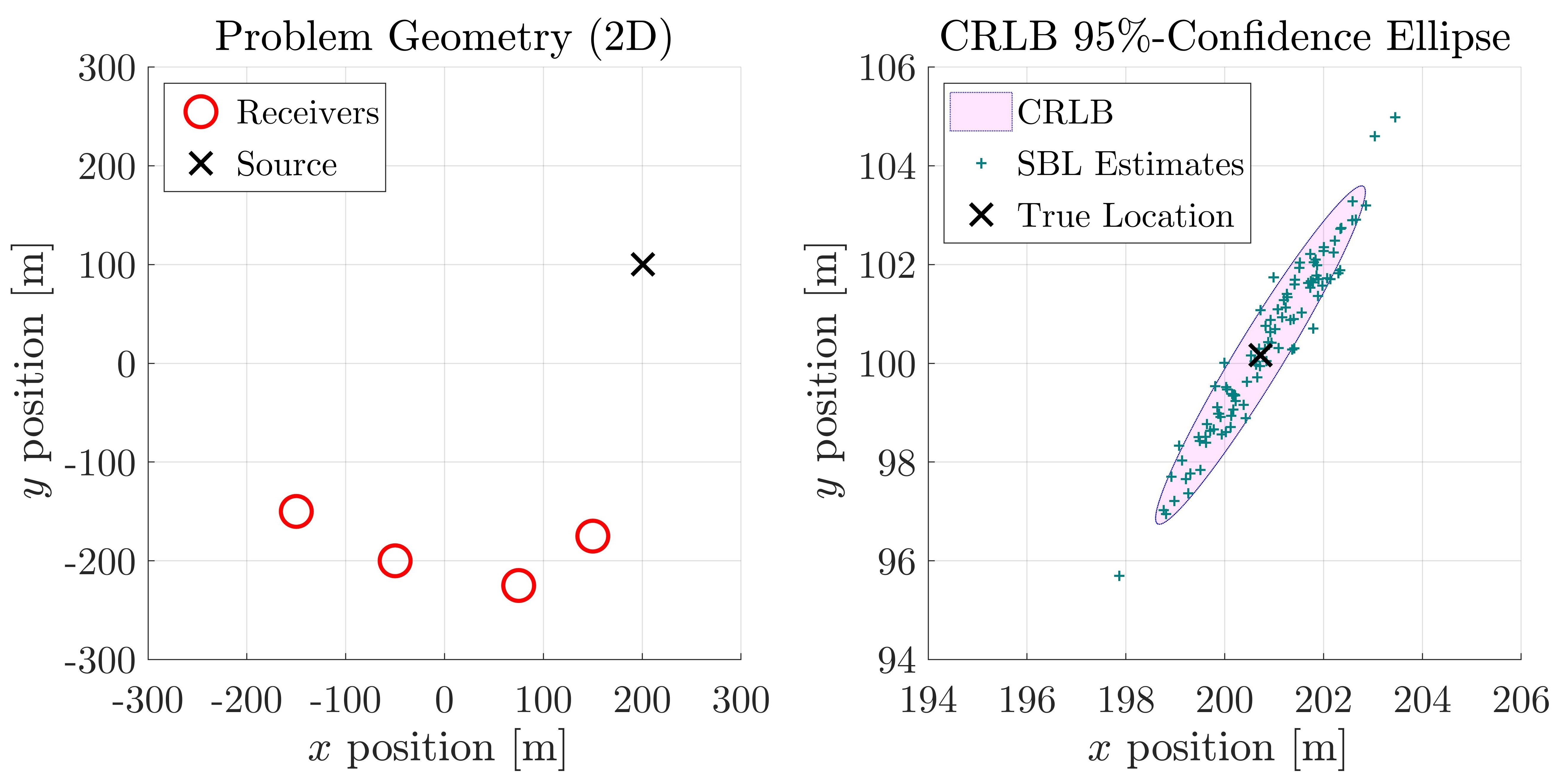
We consider a scenario with L=4𝐿4L=4 receivers, in an area with bottom depth h=100m100mh=100\;\text{m}. The locations of the receivers and the source are given in Table II. The attenuation coefficients were drawn (once, and then fixed) independently from the circularly-symmetric CN distribution, such that 𝔼[|brl|2]=1𝔼delimited-[]superscriptsubscript𝑏𝑟𝑙21\mathbb{E}\left[|b_{rl}|^{2}\right]=1, with variance 0.12superscript0.120.1^{2}. The speed of sound was set to c=1500m/s𝑐1500msc=1500\;\text{m}/\text{s}, and the sample size to N=30𝑁30N=30. We consider the case 𝓔=𝐎𝓔𝐎{\mbox{\boldmath$\mathcal{E}$}}=\mathbf{O}, such that the waveform’s DFT coefficients are s¯[k]=1Neȷϕs[k]s¯delimited-[]𝑘1𝑁superscript𝑒italic-ȷsubscriptitalic-ϕ𝑠delimited-[]𝑘\hskip 0.15625pt\hbox to0.0pt{\leavevmode\hbox{\set@color$s$}\hss}{\hskip-0.15625pt\leavevmode\hbox{\set@color$\overline{\hbox{}}$}}[k]=\frac{1}{\sqrt{N}}e^{\jmath\phi_{s}[k]}, and the phases {ϕs[k]}k=2Nsuperscriptsubscriptsubscriptitalic-ϕ𝑠delimited-[]𝑘𝑘2𝑁\{\phi_{s}[k]\}_{k=2}^{N} were drawn111111Except for the (immaterial) ϕs[1]=0subscriptitalic-ϕ𝑠delimited-[]10\phi_{s}[1]=0, due to our semi-blind setting. (once, and then fixed) independently from the uniform distribution U(0,2π)𝑈02𝜋U(0,2\pi). In this case, 𝒑^SBLsubscript^𝒑SBL\widehat{{\mbox{\boldmath$p$}}}_{\text{\tiny SBL}} is the MLE, and the CRLB accurately predicts its asymptotic variance. The received signals were generated according to (6), where the noise realization for all four sensors were taken from recordings of ocean ambient noise from the KAM11 experiment [32]. This way, we obtain a hybrid signal for this simulation, which allows us to test the validity of the bound on real ambient noise, which is potentially not CN and temporally white. Since the CRLB is informative only asymptotically (in the “small errors” regime), we set the noise variance121212We do so by first normalizing the recorded ambient noise to have unit variance, and then scale it accordingly to have the desired level of SNR. to σv2=σv2=0.1superscriptsubscript𝜎subscript𝑣2superscriptsubscript𝜎𝑣20.1\sigma_{v_{\ell}}^{2}=\sigma_{v}^{2}=0.1 for all {1,2,3,4}1234\ell\in\{1,2,3,4\}, to have an SNR of 𝒔¯22/σv2=10superscriptsubscriptdelimited-∥∥𝒔¯22superscriptsubscript𝜎𝑣210\left\lVert\hskip 0.15625pt\hbox to0.0pt{\leavevmode\hbox{\set@color${\mbox{\boldmath$s$}}$}\hss}{\hskip-0.15625pt\leavevmode\hbox{\set@color$\overline{\hbox{}}$}}\right\rVert_{2}^{2}/\sigma_{v}^{2}=10 dB.

x𝑥x [m] y𝑦y [m] z𝑧z [m] Source Position, 𝒑𝒑p 200.7240200.7240200.7240 100.1661100.1661100.1661 30.637430.637430.6374 Receiver 1, 𝒑1subscript𝒑1{\mbox{\boldmath$p$}}_{1} 150150150 175175-175 202020 Receiver 2, 𝒑2subscript𝒑2{\mbox{\boldmath$p$}}_{2} 757575 225225-225 202020 Receiver 3, 𝒑3subscript𝒑3{\mbox{\boldmath$p$}}_{3} 5050-50 200200-200 202020 Receiver 4, 𝒑4subscript𝒑4{\mbox{\boldmath$p$}}_{4} 150150-150 150150-150 202020

TABLE II: Positions of the source and the four receivers for the setting considered in Subsection VI-A, depicted in Fig. 3 (left), with Ts=103 ssubscript𝑇𝑠superscript103 sT_{s}=10^{-3}\text{ s}. Note that the source position is not located on a (discrete) grid point.
Refer to caption
Figure 3: Validation of the predicted asymptotic performance using the CRLB for the hybrid signal, containing recordings of ocean ambient noise collected in the KAM11 experiment. Left: The 222-dimensional setting of the scenario under consideration. Right: The 95%percent9595\%-confidence ellipse, as predicted by the CRLB (33), with 100100100 superimposed estimates.
Refer to caption
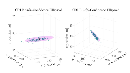
Figure 4: Two different points of views for the (same) 333-dimensional 95%percent9595\%-confidence ellipsoid based on the CRLB, with 100100100 SBL estimates superimposed (legend as in Fig. 3, right). The CRLB accurately quantifies how the variance of the proposed solution is spread in the 333-dimensional space.

Figure 3 presents the 222-dimensional setting under consideration, and the 95%percent9595\% confidence ellipse computed using the CRLB (33), with superimposed estimates 𝒑^SBLsubscript^𝒑SBL\widehat{{\mbox{\boldmath$p$}}}_{\text{\tiny SBL}} obtained for 100100100 different noise recordings. Despite the model mismatch with respect to the noise distribution, a good fit is seen between the empirical results and the predicted theoretical accuracy due to the CRLB. Figure 4 reflects the same fit in the 333-dimensional space. This not only agrees with our analytical derivation of the bound, but also provides an empirical justification for our stochastic noise model. In this regard, we note further that the hybrid signals we use allow us to essentially isolate the (potential) noise-related model mismatch effects, and test our proposed solution with respect to deviations of this sort only.

VI-B Comparison with GCC-PHAT and MFP3
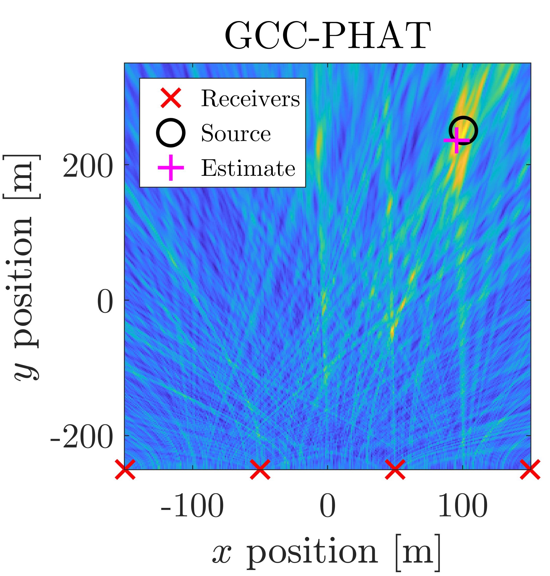
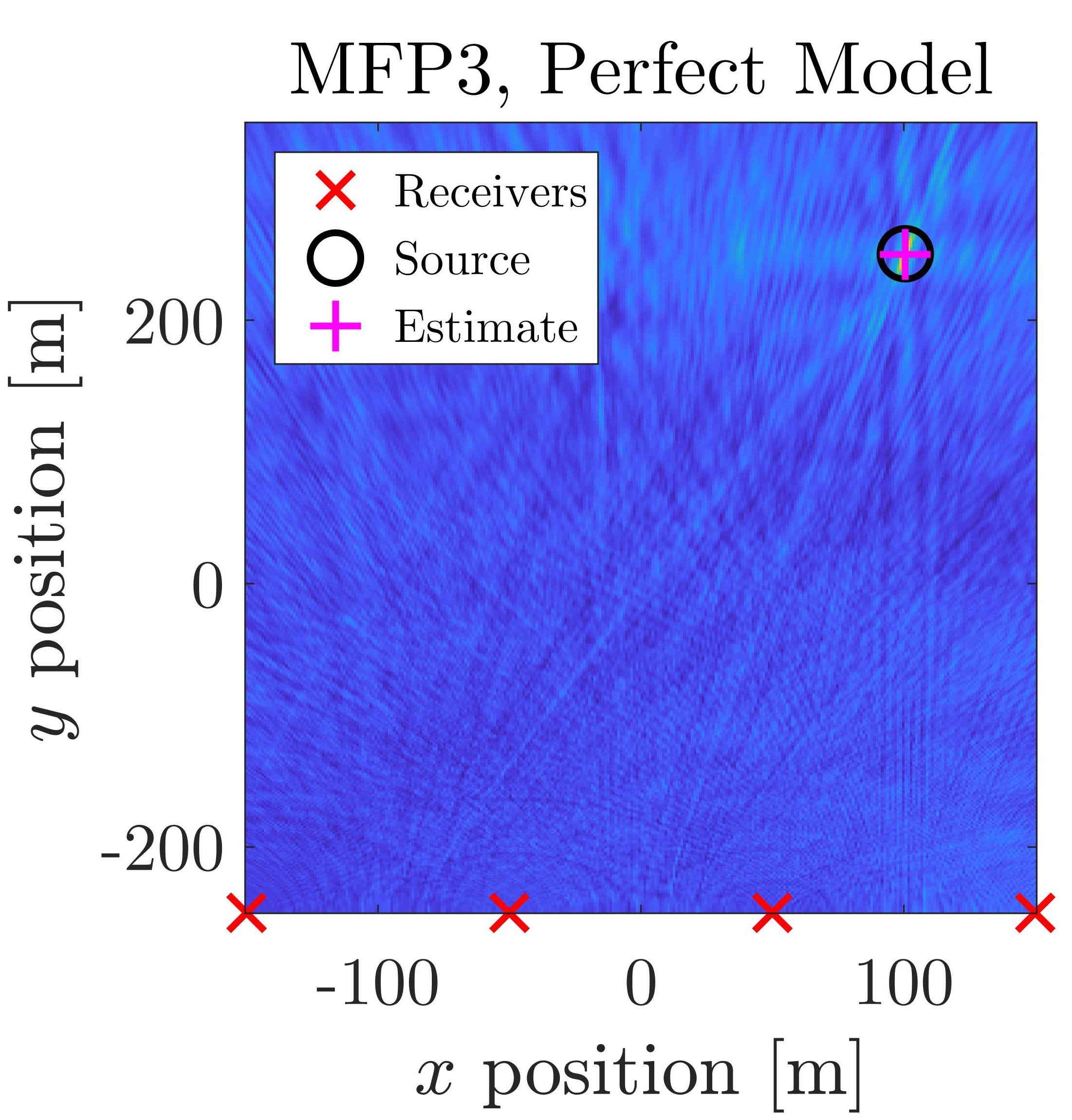
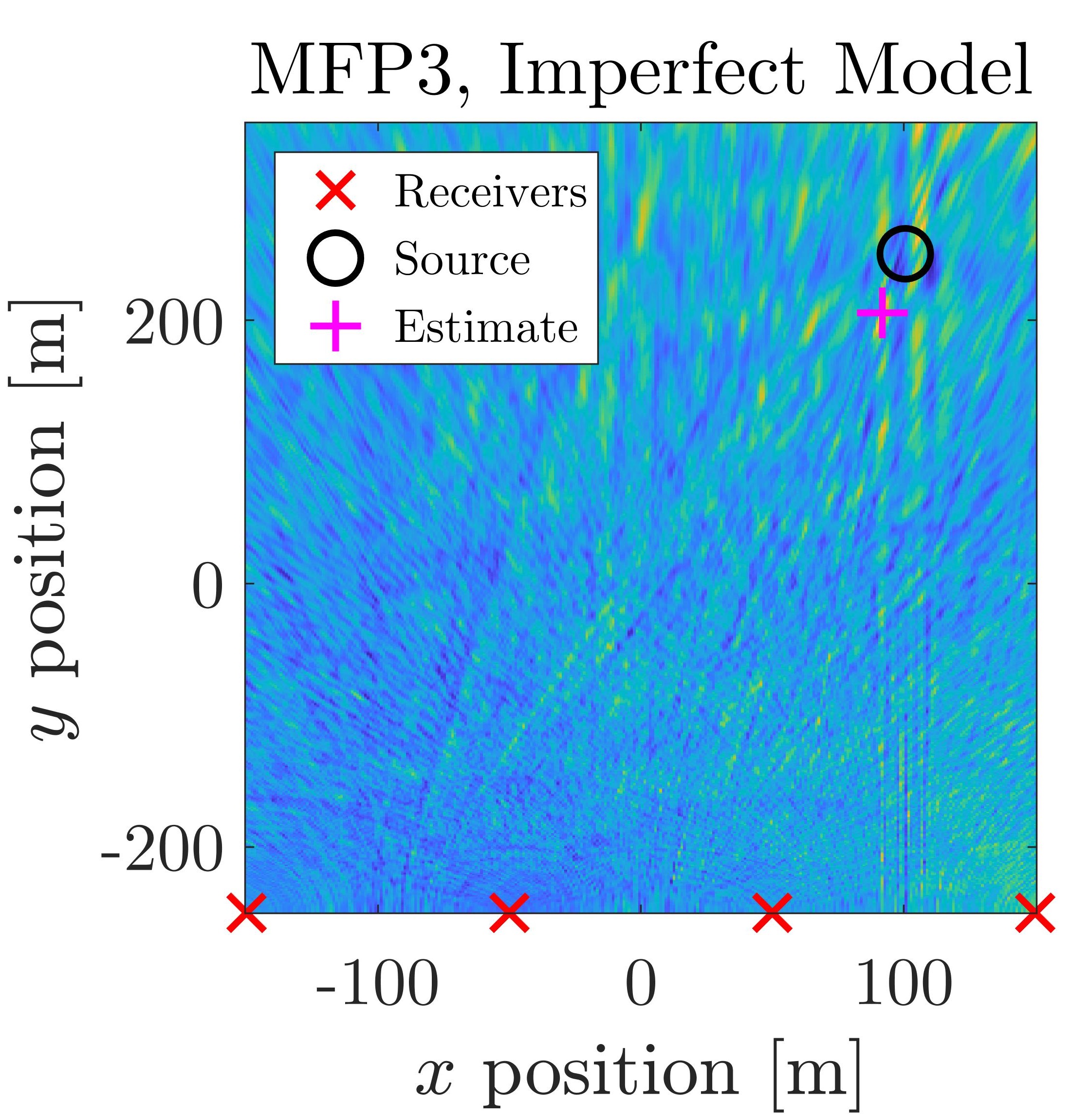
Refer to caption
(a)
Refer to caption
(b)
Refer to caption
(c)
Refer to caption
(d)
Figure 5: 222-dimensional slices at the source depth (z=zp𝑧subscript𝑧𝑝z=z_{p}) of the objective function for typical realizations at 555 dB SNR. (a) GCC-PHAT (b) MFP3 with perfect model (c) MFP3 with unknown phases of 𝒃1,𝒃Lsubscript𝒃1subscript𝒃𝐿{\mbox{\boldmath$b$}}_{1}\,\ldots,{\mbox{\boldmath$b$}}_{L} (d) SBL. Evidently, GCC-PHAT and MFP3 without perfect knowledge are considerably more fragile than the proposed method, which is similar to MFP3 with perfect knowledge with respect to stability, at the cost of a higher variance.
Refer to caption
Figure 6: RMS miss distance vs. SNR, for T=100𝑇100T=100. At very low SNR, all methods perform poorly. As the SNR increases, GCC-PHAT improves only moderately, while SBL improves significantly.
Refer to caption
Figure 7: RMS miss distance vs. ϵitalic-ϵ\epsilon, quantifying a deviation from the physical model, for T=100𝑇100T=100 and σv2=0.1superscriptsubscript𝜎subscript𝑣20.1\sigma_{v_{\ell}}^{2}=0.1. MFP3 is sensitive to such model deviations, while GCC-PHAT and SBL are robust.
Refer to caption
Figure 8: RMS miss distance vs. β𝛽\beta, the LOS attenuation coefficient of receivers =2,323\ell=2,3, for T=100𝑇100T=100 and σv2=0.1superscriptsubscript𝜎subscript𝑣20.1\sigma_{v_{\ell}}^{2}=0.1. Our proposed SBL offer the best accuracy-stability balance out of the three methods.

We now compare the proposed SBL method with MFP3 and the GCC-PHAT localization methods. In this simulated experiment, we consider the setup depicted in Fig. 5, namely a linear deployment of the receivers. Such a deployment is conceivable for naval defense purposes near the shoreline, or harbor monitoring [44]. The positions of the source and the receivers, and all relevant system and environmental parameters are given in Table III. The source’s DFT coefficients s¯[k]s¯delimited-[]𝑘\hskip 0.15625pt\hbox to0.0pt{\leavevmode\hbox{\set@color$s$}\hss}{\hskip-0.15625pt\leavevmode\hbox{\set@color$\overline{\hbox{}}$}}[k], as well as the noise realizations { ¯v[k]}subscript ¯vdelimited-[]𝑘\{\hbox to0.0pt{\hskip 0.103pt\leavevmode\hbox{\set@color$\overline{\hbox{}}$}\hss}{\leavevmode\hbox{\set@color$v$}}_{\ell}[k]\}, were drawn independently from the standard CN distribution in each trial. The noise variance of the \ell-th receiver is set as σv2=σv2𝒃2superscriptsubscript𝜎subscript𝑣2superscriptsubscript𝜎𝑣2superscriptnormsubscript𝒃2\sigma_{v_{\ell}}^{2}=\sigma_{v}^{2}\cdot\|{\mbox{\boldmath$b$}}_{\ell}\|^{2}, and the SNR is defined here as 𝔼[|s¯[k]|2]/σv2=1/σv2𝔼delimited-[]superscripts¯delimited-[]𝑘2superscriptsubscript𝜎𝑣21superscriptsubscript𝜎𝑣2\mathbb{E}\left[|\hskip 0.15625pt\hbox to0.0pt{\leavevmode\hbox{\set@color$s$}\hss}{\hskip-0.15625pt\leavevmode\hbox{\set@color$\overline{\hbox{}}$}}[k]|^{2}\right]/\sigma_{v}^{2}=1/\sigma_{v}^{2}. All empirical results presented in this subsection are based on averaging 104superscript10410^{4} independent trials.

x𝑥x [m] y𝑦y [m] z𝑧z [m] Source Position, 𝒑𝒑p 100.5976100.5976100.5976 250.5837250.5837250.5837 30.113130.113130.1131 Receiver 1, 𝒑1subscript𝒑1{\mbox{\boldmath$p$}}_{1} 150150150 250250-250 101010 Receiver 2, 𝒑2subscript𝒑2{\mbox{\boldmath$p$}}_{2} 505050 250250-250 151515 Receiver 3, 𝒑3subscript𝒑3{\mbox{\boldmath$p$}}_{3} 5050-50 250250-250 202020 Receiver 4, 𝒑4subscript𝒑4{\mbox{\boldmath$p$}}_{4} 150150-150 250250-250 252525 c=1535𝑐1535c=1535 m/s, κb=0.85subscript𝜅𝑏0.85\kappa_{b}=0.85, h=100100h=100 m, N=100𝑁100N=100, Ts=0.001subscript𝑇𝑠0.001T_{s}=0.001 s

TABLE III: The setting considered in Subsection VI-B.

We first compare the localization accuracies of the methods for different SNRs. Figure 8 presents the root mean squared (RMS) miss distance, i.e., the square root of (26), vs. the SNR for each method. A 2D slice at the receiver’s depth of the objective functions of each of the algorithms for a typical realization at 555 dB SNR is given in Fig. 5. For MFP3, we show the performance obtained with perfect knowledge of the channel (“Perfect Model”), i.e., when 𝒃1,,𝒃Lsubscript𝒃1subscript𝒃𝐿{\mbox{\boldmath$b$}}_{1},\ldots,{\mbox{\boldmath$b$}}_{L} and κbsubscript𝜅𝑏\kappa_{b} are known exactly; and when this perfect knowledge is accurate except for the phases of 𝒃1,,𝒃Lsubscript𝒃1subscript𝒃𝐿{\mbox{\boldmath$b$}}_{1},\ldots,{\mbox{\boldmath$b$}}_{L} (“Imperfect Model”), which are drawn independently from U(0,2π)𝑈02𝜋U(0,2\pi). As observed, although GCC-PHAT improves when the SNR increases, it essentially cannot cope well—in a 333-dimensional space optimization—with the addition of the surface and bottom reflections. It is also seen the MFP3 is highly sensitive to deviations from the assumed channel response. In contrast, such deviations are completely transparent to SBL, as it considers these parameters as unknown, and implicitly optimizes over them jointly with all the other unknowns (see (36), Appendix A). The robustness at the moderate cost in performance relative to MFP3 is evident. Note that MFP3’s superior performance is guaranteed only asymptotically, in agreement with the results in Fig. 8.

Next, we compare the performances of the three different methods with respect to perturbations in the expected channel attenuations, as prescribed by the physical model (9)–(11). This form of model mismatch is likely to occur in practice due to nonidealities131313Within the three-ray model. Of course, in practice there are more modeling mismatch factors due to the simplified three-ray model. The effects of some of these nonidealities will be evaluated in the next experiment, where we apply our method to real data, and demonstrate successful localization. (e.g., inaccurate prior knowledge of κbsubscript𝜅𝑏\kappa_{b}). Formally, we model these deviations by generating the channel attenuation coefficients as

br(ϵ)=(1ϵγr)breȷ2πϵφr,r{1,2,3},{1,2,3,4},formulae-sequencesubscript𝑏𝑟italic-ϵ1italic-ϵsubscript𝛾𝑟subscript𝑏𝑟superscript𝑒italic-ȷ2𝜋italic-ϵsubscript𝜑𝑟formulae-sequence𝑟1231234\begin{gathered}b_{r\ell}(\epsilon)=(1-\epsilon\cdot\gamma_{r\ell})b_{r\ell}\cdot e^{\jmath 2\pi\epsilon\cdot\varphi_{r\ell}},\\ r\in\{1,2,3\},\;\ell\in\{1,2,3,4\},\end{gathered} (34)

where {γrU(0,0.5)}similar-tosubscript𝛾𝑟𝑈00.5\{\gamma_{r\ell}\sim U(0,0.5)\} and {φrU(0,1)}similar-tosubscript𝜑𝑟𝑈01\{\varphi_{r\ell}\sim U(0,1)\} are independent. In (34), ϵ[0,1]italic-ϵ01\epsilon\in[0,1] is a parameter controlling the deviation from the physical model, where ϵ=0italic-ϵ0\epsilon=0 corresponds to no deviation from (9)–(11).

Figure 8 presents the RMS miss distance vs. ϵitalic-ϵ\epsilon. As expected, we observe an overall accuracy-robustness superiority of SBL relative to the competing algorithms. While MFP3 is superior when perfect knowledge of the channel parameters κb,𝒃1,,𝒃Lsubscript𝜅𝑏subscript𝒃1subscript𝒃𝐿\kappa_{b},{\mbox{\boldmath$b$}}_{1},\ldots,{\mbox{\boldmath$b$}}_{L} is available, SBL is inherently indifferent to deviations from their ideal physical values. GCC-PHAT is also robust to such deviations, but completely ignores (by design) the multipath channel, and therefore cannot exploit additional signal components, such as surface and bottom reflections.

In the last simulation for this setup, we model the effect of a potential occluder between some of the receivers and the source. Specifically, for the second and third receivers (i.e., at 𝒑2subscript𝒑2{\mbox{\boldmath$p$}}_{2} and 𝒑3subscript𝒑3{\mbox{\boldmath$p$}}_{3}), we introduce an attenuation coefficient β[0,1]𝛽01\beta\in[0,1] to the LOS components, such that

b1(β)=βb1eȷ2π(1β)φ1,{2,3}.formulae-sequencesubscript𝑏1𝛽𝛽subscript𝑏1superscript𝑒italic-ȷ2𝜋1𝛽subscript𝜑123b_{1\ell}(\beta)=\beta\cdot b_{1\ell}\cdot e^{\jmath 2\pi(1-\beta)\varphi_{1\ell}},\ell\in\{2,3\}. (35)

When β=1𝛽1\beta=1, there is no occlusion, and when β=0𝛽0\beta=0, the LOS components of receivers =2,323\ell=2,3 are completely lost. The phase perturbation models the interaction with the occluder.

Figure 8 presents the RMS miss distance vs. β𝛽\beta. It is observed that the accuracy obtained by GCC-PHAT is on the same order of the distances (25similar-toabsent25\sim 25m) corresponding to the time delays between the LOS and NLOS components. This level of accuracy is stable, but is not satisfactory for an SNR level of 101010 dB (here, σv2=0.1superscriptsubscript𝜎𝑣20.1\sigma_{v}^{2}=0.1). It is also seen that in the absence of a modeling error (i.e., β=1𝛽1\beta=1), MFP3 attains the highest accuracy. However, deviations from the ideal signal model, in the form of occluded LOS components of two receivers, inflict a severe performance deterioration.

As we have demonstrated in Fig. 5(c) and Fig. 8, when MFP3 is actually mis-matched, it could perform even worse than what is presented in Fig. 8. Still, even in this setting, our method exhibits the best accuracy-stability trade-off.

VI-C Experimental Results

Refer to caption
Figure 9: A picture of our water tank. Our testbed provides high frequency (200400200400200-400 kHz) noisy acoustic data from a complex reverberant environment.

We now demonstrate the performance of our proposed method on acoustic data acquired in our water tank testbed—the high frequency autonomous acoustic tank. This system, presented in Fig. 9, is (roughly) of size 25cm×32cm×15cm25cm32cm15cm25\;\text{cm}\times 32\;\text{cm}\times 15\;\text{cm}, and enables us to create a controlled and challenging setting for frequency-scaled underwater localization.

Although the water tank environment is only a scale model of a shallow-water environment, it nevertheless poses a challenging scenario. In addition to the modeled bottom and surface reflections, the water tank has four additional sides, that are reflective boundaries. These thin plastic boundaries are highly reflective, so that the test environment is highly reverberant, giving rise to a rich multipath channel. In particular, the magnitudes of the unmodeled reflections are comparable to the modeled ones in our three-ray model.

In this experiment, the source is transmitting a Gaussian pulse at a carrier frequency of 280280280 kHz, and the speed of sound in the water tank is c=1485𝑐1485c=1485 m/sms\text{m}/\text{s}. To maintain consistency across different trials, the source and receivers were set at the same depth. In this case, spatial diversity in the depth-direction is limited, hence we assume here that the source’s depth is known, and approach this 222-dimensional problem.

The received signals were sampled at 222 GHz. Before applying the localization method, the signals were decimated by a factor of 2×1032superscript1032\times 10^{3}, to obtain 111 MHz bandwidth signals. For each setting, in which the source and receivers were static, the observation interval was 0.50.50.5 ms long. More technical details are given in the supplementary materials.

Figs. 10, 11 and 12 present the objective functions of GCC-PHAT, MFP3 and the proposed method, respectively, for three different source locations. Here, the search area is a 30×30cm23030superscriptcm230\times 30\;\text{cm}^{2} square, centered around the first receiver. Note that we intentionally did not align the search area with the one dictated by the boundaries of the tank, since we assume that such prior knowledge is unavailable as in a real problem setting.

Refer to caption
Figure 10: GCC-PHAT experimental results based on acoustic measurements acquired in the water tank using the system presented in Fig. 9.
Refer to caption
Figure 11: MFP3 experimental results based on acoustic measurements acquired in the water tank using the system presented in Fig. 9.
Refer to caption
Figure 12: SBL experimental results based on acoustic measurements acquired in the water tank using the system presented in Fig. 9.

As was observed in the simulations, it is seen that in the presence of strong multipath, GCC-PHAT suffers from the worst performance degradation, and MFP3 is the most accurate, best exploiting the environmental prior knowledge. SBL is less accurate than MFP3, but still provides reasonable estimates in the vicinity of the source’s true location.

Next, we repeat the experiment but now with the presence of an unknown object—a cylinder, stretching from the bottom to the surface of the tank, placed in the area between the source and the receivers, as depicted in Figs. 1315. This unknown feature causes severe model mismatch; critically, if it blocks the LOS between the source and a receiver, then all the three modeled rays—LOS, and surface and bottom reflections—are essentially blocked. A flexible algorithm can in principle select (possibly implicitly) which receivers to use, and would be able to reject uninformative measurements, such as the ones acquired by a receiver “viewing” the occluded scenery.

Figures 13, 14 and 15, presenting the objective functions of GCC-PHAT, MFP3 and SBL, respectively, for the same scenarios but with an occluder, corroborate the robustness of the SBL method. It is seen that GCC-PHAT and MFP3 are fragile when such unknown environmental features are present. The SBL method, which exhibits robustness in the presence of the occluder, is still able to localize the source. Since the attenuation coefficients are considered to be unknown, and are implicitly estimated (36), a perfectly valid estimated value (for some of them) is a value close or equal to zero. This essentially means that the SBL assigns different weights to measurements from different receivers, thus implicitly choosing to effectively ignore the less informative data acquired by receivers with occluded scenery.

Refer to caption
Figure 13: GCC-PHAT experimental results based on acoustic measurements acquired in the water tank using the system presented in Fig. 9, with the presence of an unknown occluder (cylinder), modeling an effect of inaccurate environmental prior knowledge.
Refer to caption
Figure 14: MFP3 experimental results based on acoustic measurements acquired in the water tank using the system presented in Fig. 9, with the presence of an unknown occluder (cylinder), modeling an effect of inaccurate environmental prior knowledge.
Refer to caption
Figure 15: SBL experimental results based on acoustic measurements acquired in the water tank using the system presented in Fig. 9, with the presence of an unknown occluder (cylinder), modeling an effect of inaccurate environmental prior knowledge.

VII Discussion and Extensions

A natural extension of the direct localization problem that we considered, is to the case of multiple sources and/or a more complex channel model, which is beyond the scope of this paper and is left for future work. However, in this section we outline some key challenges of this setting to motivate this non-trivial extended problem. We then discuss the potential use of the SBL estimator in such scenarios, and point out important aspects of identifiability. Before addressing these topics, we first discuss some system design considerations for the particular setting described in Section II.

VII-A System Design Considerations

For given, limited resources, one may be interested in enhancing the performance of a system as much as possible with respect to the available degrees of freedom. In the specific case of our localization problem, performance can be understood as accuracy (e.g., in terms of (26)), and resources, perhaps, as the number of receivers, L𝐿L.141414which are also the number of sensors in our formulation. While we defer the formulation of this notion into a well-defined problem (possibly using some function of the bound (33)) to future work, we comment on the important related aspects of the topology and the number of receivers.

Recall that a single receiver, equipped with a single sensor, receives (in general) three signal components, two of which are reflected from the surface and the bottom, which are respectively above and under the receiver. Thus, environmental knowledge regarding the position of the surface and the bottom is equivalent, in some sense, to having additional virtual receivers (e.g., [45]) above and under the surface and the bottom, respectively. In this respect, a single receiver already provides some vertical spatial diversity. Still, due to the blind nature of the problem, in which the emitted waveform and the channel coefficients are unknown, the information from a single sensor is insufficient for localization.

However, two sensors already contain six signal components, and can in principle contain sufficient information for localization. Intuitively, breaking the symmetry “as much as possible” relative to the environment in which the system is deployed would lead to better performance. In the two receivers case, placing the second receiver in a different horizontal location than the first would lead to an increased horizontal spatial diversity, which would in turn lead to enhanced performance. The principle of increasing spatial diversity with a fixed resources allocation can be formulated in some settings (e.g., [46]), and provides guidance and intuition for the design of a sensors network spatial distribution. For example, one may consider deploying a linear network of sensors obliquely relative to the surface.

VII-B Key Challenges in Extended Models

Incorporating multiple sources into the 3-ray signal model (5) changes the interplay between the (consequently increased) number of unknown parameters. As a result, it is no longer clear whether a simplified, efficiently computable expression for the objective function—as (22) in Proposition 1—can be obtained. Recall that this has a significant effect on the overall computational complexity of the method.

Moreover, assume that there are M𝑀M sources to be localized (where M𝑀M is known), and further assume that we have obtained such a simplified, computationally efficient expression for the objective function, which is a function of the sources’ positions only, denoted by, say, 𝒑(1),,𝒑(M)3×1superscript𝒑1superscript𝒑𝑀superscript31{\mbox{\boldmath$p$}}^{(1)},\ldots,{\mbox{\boldmath$p$}}^{(M)}\in\mathbb{R}^{3\times 1}. At this point, in order to obtain the optimal direct localization solution (in the sense of the extended criterion of (15)) for all M𝑀M sources, one is required to solve a 3M3𝑀3M-dimensional nonlinear optimization problem, which may well be non-convex. Consequently, even for M=2𝑀2M=2 sources, this is already difficult with a naive extension of our current proposed method, as it would require a 666-dimensional grid search (referring to the first step of the proposed solution), which is infeasible for reasonable resolutions. Hence, a different approach is perhaps required in order to solve the multiple sources direct localization problem.

Focusing again on the single source case, one may consider an extended K𝐾K-ray model (with K>3𝐾3K>3), assuming it would accurately describe the signal propagation, such that the K𝐾K rays include primary and second- and higher-order reflections. In that case, the performance (i.e., accuracy) improvement would be due to an increased effective/post-processing SNR. This can be understood from the interpretation given in Subsection IV-A, where the SBL method is seen as an implicit way to coherently add all the K𝐾K reflections from all L𝐿L sensors.

However, and since the ray-based propagation model is an approximation, while the deviations from the 333 primary rays can be small, the aggregated approximation errors in the time-delays of the higher-order reflections are likely to no longer be negligible. In that case, on top of additional computational burden, a naive extension of the current approach might yield a more fragile estimator, which is sensitive to model mismatch. The challenging task of exploiting more complex propagation-related phenomena for enhanced, computationally attractive direct localization remains to be explored in future work.

VII-C SBL as a Solution for Multiple Sources

Notwithstanding the above, our proposed algorithm can still be used for multiple sources localization as a sub-optimal, yet computationally feasible solution. Indeed, (22) can be viewed as a spatial quasi-likelihood map (as a function of 𝒑𝒑p), whose M𝑀M highest maxima correspond to the M𝑀M points in space, where sources are most likely to be present (under the mismatched model (5), treating, for each source, all the other M1𝑀1M-1 sources as additive noise). While providing analytical guarantees for this case is beyond the scope of the current work, using the Matlab package provided in the supplementary material, one could easily verify that the SBL method still serves as a viable localization solution for this extended setting.

Given any set of parameters that describe a particular localization problem (i.e., bottom depth, locations of the receivers, etc.), the model (5) is guaranteed to be identifiable when the FIM is nonsingular, namely det(𝑱(𝜽))0𝑱𝜽0\det\left({\mbox{\boldmath$J$}}({\mbox{\boldmath$\theta$}})\right)\neq 0, and (33) is finite. However, when using the SBL for localization of multiple source (i.e., under mismatched model) as described above, this is obviously no longer true. Indeed, as least theoretically, there are certain “special” (however somewhat extreme) scenarios in which the sources not only could not be localized (reliably, or at all), but may also “disappear” from the resulting heatmap.

To illustrate this, consider the following case, which is depicted in Fig. 16. Assume, for example, that L𝐿L receivers are all deployed at the same depth h/22h/2 in a linear structure, namely z=z0=h/2,y=y0formulae-sequencesubscript𝑧subscript𝑧02subscript𝑦subscript𝑦0z_{\ell}=z_{0}=h/2,y_{\ell}=y_{0} and x=x0+Δ(1)subscript𝑥subscript𝑥0Δ1x_{\ell}=x_{0}+\Delta(\ell-1) for all {1,,L}1𝐿\ell\in\{1,\ldots,L\}, where ΔΔ\Delta is the spacing between the receivers. Now, further assume that two sources are present, such that the second source is located at the same horizontal location as the first, but is located symmetrically about the half depth h/22h/2 relative to the first. That is, if the first source is at 𝒑=(xp,yp,zp)𝒑subscript𝑥𝑝subscript𝑦𝑝subscript𝑧𝑝{\mbox{\boldmath$p$}}=(x_{p},y_{p},z_{p}), the second is at 𝒑~=(xp,yp,hzp)~𝒑subscript𝑥𝑝subscript𝑦𝑝subscript𝑧𝑝\widetilde{{\mbox{\boldmath$p$}}}=(x_{p},y_{p},h-z_{p}). Finally, assume that an occluding object is present, such that (only) all LOS components at all L𝐿L receivers are blocked from both of the sources. Denoting by R~2,R~3subscript~𝑅2subscript~𝑅3\widetilde{R}_{2\ell},\widetilde{R}_{3\ell} the distances traveled by the NLOS surface and bottom associated rays, respectively, from the second source, it readily follows from (2)–(4) that R~2=R3,R~3=R2formulae-sequencesubscript~𝑅2subscript𝑅3subscript~𝑅3subscript𝑅2\widetilde{R}_{2\ell}=R_{3\ell},\widetilde{R}_{3\ell}=R_{2\ell}, hence

τ2(𝒑)=τ3(𝒑~),τ3(𝒑)=τ2(𝒑~).formulae-sequencesubscript𝜏2𝒑subscript𝜏3~𝒑subscript𝜏3𝒑subscript𝜏2~𝒑\tau_{2\ell}({\mbox{\boldmath$p$}})=\tau_{3\ell}(\widetilde{{\mbox{\boldmath$p$}}}),\quad\tau_{3\ell}({\mbox{\boldmath$p$}})=\tau_{2\ell}(\widetilde{{\mbox{\boldmath$p$}}}).

In this case, if κb=1subscript𝜅𝑏1\kappa_{b}=1 (of (11)), and if the two sources are collaborating and coordinated, then by transmitting the same waveform, they are essentially “acoustically invisible” (under the three ray model). Indeed, if we denote the waveform of the second source by s~(t)=s(t)~𝑠𝑡𝑠𝑡\widetilde{s}(t)=s(t), the baseband-converted signal from the \ell-th receiver (as in (5)) would then be

x[n]=subscript𝑥delimited-[]𝑛absent\displaystyle x_{\ell}[n]= r=23brs(tτr(𝒑))|t=nTs+limit-fromevaluated-atsuperscriptsubscript𝑟23subscript𝑏𝑟𝑠𝑡subscript𝜏𝑟𝒑𝑡𝑛subscript𝑇𝑠\displaystyle\sum_{r=2}^{3}b_{r\ell}\left.s\left(t-\tau_{r\ell}({\mbox{\boldmath$p$}})\right)\right|_{t=nT_{s}}+
r=23b~rs~(tτr(𝒑~))|t=nTs=r=23brs(tτr(𝒑))|t=nTs+v[n]=v[n],subscriptevaluated-atsuperscriptsubscript𝑟23subscript~𝑏𝑟~𝑠𝑡subscript𝜏𝑟~𝒑𝑡𝑛subscript𝑇𝑠absentevaluated-atsuperscriptsubscript𝑟23subscript𝑏𝑟𝑠𝑡subscript𝜏𝑟𝒑𝑡𝑛subscript𝑇𝑠subscript𝑣delimited-[]𝑛subscript𝑣delimited-[]𝑛\displaystyle\underbrace{\sum_{r=2}^{3}\widetilde{b}_{r\ell}\left.\widetilde{s}\left(t-\tau_{r\ell}(\widetilde{{\mbox{\boldmath$p$}}})\right)\right|_{t=nT_{s}}}_{=\,-\sum_{r=2}^{3}b_{r\ell}\left.s\left(t-\tau_{r\ell}(\text{\boldmath$p$})\right)\right|_{t=nT_{s}}}+v_{\ell}[n]=v_{\ell}[n],

since b~2=1R3=b3subscript~𝑏21subscript𝑅3subscript𝑏3\widetilde{b}_{2\ell}=\frac{-1}{R_{3\ell}}=-b_{3\ell} and b~3=1R2=b2subscript~𝑏31subscript𝑅2subscript𝑏2\widetilde{b}_{3\ell}=\frac{1}{R_{2\ell}}=-b_{2\ell}, and we recall that due to the occluder, b1=b~1=0subscript𝑏1subscript~𝑏10b_{1\ell}=\widetilde{b}_{1\ell}=0 for all {1,,L}1𝐿\ell\in\{1,\ldots,L\}. Thus, only noise is observed, and all the information is lost.
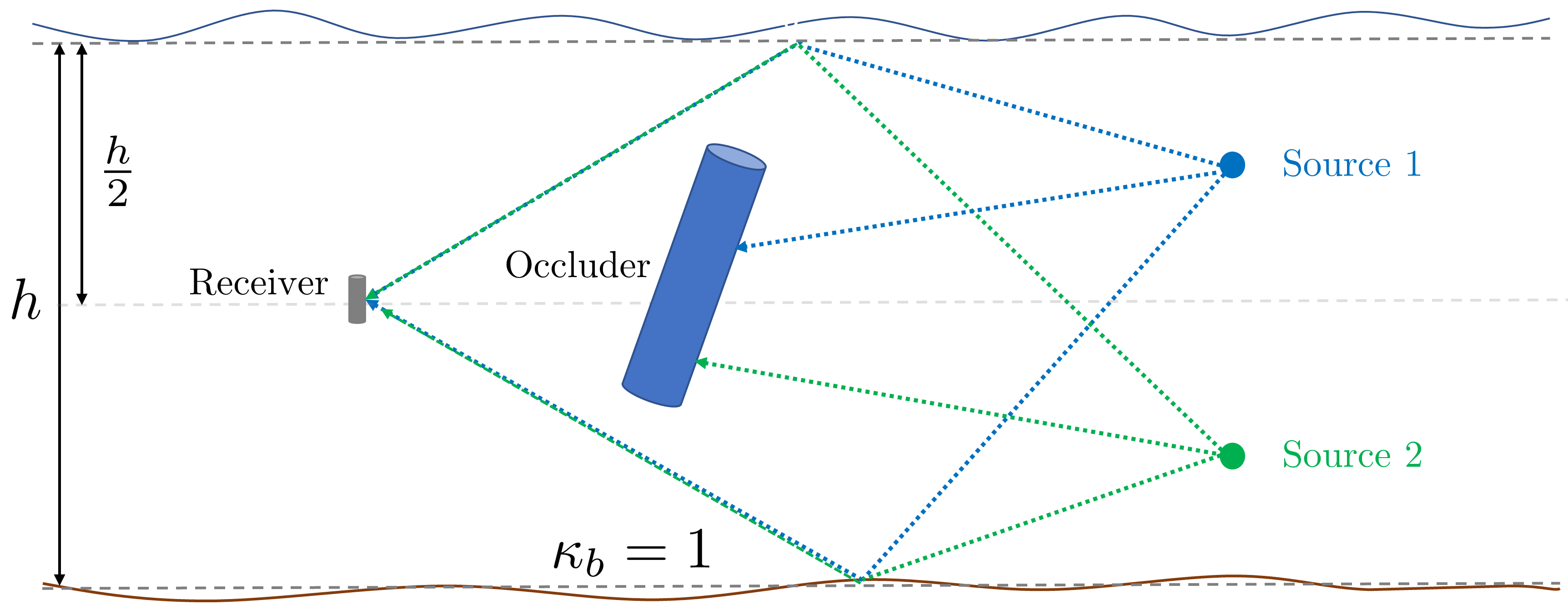
Refer to caption
Figure 16: A 222-dimensional illustration of the special case described in Subsection VII-C, wherein the sources are “acoustically invisible” in terms of the three-ray model, and cannot be localized by the SBL estimator.

While the scenario above can certainly inspire underwater acoustic warfare techniques devised against single-source methods like the SBL, it nonetheless describes an extreme case of a perfectly tailored setting, where several conditions, which are exceptionally difficult to ensure, are fulfilled simultaneously. Therefore, and while this is only one example of a potential failure mechanism of the proposed method when used for localization of multiple sources, one may still gain a general impression of what should happen in order for SBL to completely fail in this setting. Generally, when the sources are not collaborating/coordinated and/or the symmetry is broken (e.g., by a non-regular deployment of the receivers), it is reasonable that the proposed method would still provide reliable localization for multiple sources.

VIII Concluding remarks

In the general context of underwater acoustics, based on the three-ray propagation model, we presented a semi-blind localization method, which incorporates environmental knowledge. A closed-form expression for the objective function was derived, along with an equivalent expression, which is more computationally appealing. Thanks to additional degrees of freedom in our model, the proposed method is more robust than its MFP counterpart, and can successfully localize a source in the absence of LOS components. Further, it exhibits stable performance enhancement with respect to methods modeling only LOS components, such as GCC-PHAT.

Since the proposed method is able to coherently “collect” three signal components from each sensor, the post-processing SNR is consequently higher than any LOS-based method, which collect only one. This way, a given level of localization accuracy can generally be attained with shorter observation intervals. In turn, it is easier to incorporate the SBL method within an appropriate tracking algorithm (such as Kalman filtering), allowing for a more general framework that localizes the source and tracks its movement, assuming the source’s velocity is sufficiently low. As a topic for future research, in such cases it may be possible to develop a computationally efficient update scheme for the objective function (23), based on eigenvalue perturbation theory. Another direction for future research, that is of great practical interest, is to apply coarse quantization to the collected data [47], thus reducing the required bandwidth for communication between the different receivers. The above is also true for the potential extensions for multiple sources, and for extended propagation models.

IX Acknowledgement

The authors are grateful to James Preisig for helpful discussions, and for providing the KAM11 recordings.

Appendix A Proof of Proposition 1

Proof.

Using the identity Diag(𝑫(𝒑)𝒃)𝒔¯= ¯𝑺𝑫𝒃Diagsubscript𝑫𝒑subscript𝒃𝒔¯subscript ¯𝑺𝑫subscript𝒃\operatorname{Diag}\left({\mbox{\boldmath$D$}}_{\ell}({\mbox{\boldmath$p$}}){\mbox{\boldmath$b$}}_{\ell}\right)\hskip 0.15625pt\hbox to0.0pt{\leavevmode\hbox{\set@color${\mbox{\boldmath$s$}}$}\hss}{\hskip-0.15625pt\leavevmode\hbox{\set@color$\overline{\hbox{}}$}}=\hbox to0.0pt{\hskip 0.85414pt\leavevmode\hbox{\set@color$\overline{\hbox{}}$}\hss}{\leavevmode\hbox{\set@color${\mbox{\boldmath$S$}}$}}{\mbox{\boldmath$D$}}_{\ell}{\mbox{\boldmath$b$}}_{\ell}, it is easily seen that, for every {1,,L}1𝐿\ell\in\{1,\ldots,L\}, C~SBL(𝒑,𝒔¯,𝑩)subscript~𝐶SBL𝒑𝒔¯𝑩\widetilde{C}_{\text{\tiny SBL}}({\mbox{\boldmath$p$}},\hskip 0.15625pt\hbox to0.0pt{\leavevmode\hbox{\set@color${\mbox{\boldmath$s$}}$}\hss}{\hskip-0.15625pt\leavevmode\hbox{\set@color$\overline{\hbox{}}$}},{\mbox{\boldmath$B$}}) of (16) is minimized with respect to 𝒃subscript𝒃{\mbox{\boldmath$b$}}_{\ell} by

𝒃^=(( ¯𝑺𝑫)H ¯𝑺𝑫)1( ¯𝑺𝑫)H ¯𝒙,subscript^𝒃superscriptsuperscriptsubscript ¯𝑺𝑫Hsubscript ¯𝑺𝑫1superscriptsubscript ¯𝑺𝑫Hsubscript ¯𝒙\widehat{{\mbox{\boldmath$b$}}}_{\ell}=\left(\left(\hbox to0.0pt{\hskip 0.85414pt\leavevmode\hbox{\set@color$\overline{\hbox{}}$}\hss}{\leavevmode\hbox{\set@color${\mbox{\boldmath$S$}}$}}{\mbox{\boldmath$D$}}_{\ell}\right)^{\mathrm{H}}\hbox to0.0pt{\hskip 0.85414pt\leavevmode\hbox{\set@color$\overline{\hbox{}}$}\hss}{\leavevmode\hbox{\set@color${\mbox{\boldmath$S$}}$}}{\mbox{\boldmath$D$}}_{\ell}\right)^{-1}\left(\hbox to0.0pt{\hskip 0.85414pt\leavevmode\hbox{\set@color$\overline{\hbox{}}$}\hss}{\leavevmode\hbox{\set@color${\mbox{\boldmath$S$}}$}}{\mbox{\boldmath$D$}}_{\ell}\right)^{\mathrm{H}}\hbox to0.0pt{\hskip 0.35762pt\leavevmode\hbox{\set@color$\overline{\hbox{}}$}\hss}{\leavevmode\hbox{\set@color${\mbox{\boldmath$x$}}$}}_{\ell}{,} (36)

assuming151515We ignore the extreme, unrealistic cases in which 𝑫subscript𝑫{\mbox{\boldmath$D$}}_{\ell} are not full rank, which occur only for very specific settings of the receivers’ and source’s positions. Nonetheless, the initial optimization is performed via a grid search, hence we can discard points giving rise to these rare, singular settings. rank(𝑫)=3ranksubscript𝑫3\text{rank}\left({\mbox{\boldmath$D$}}_{\ell}\right)=3 for all {1,,L}1𝐿\ell\in\{1,\ldots,L\} hereafter. Substituting 𝑩^[𝒃^1𝒃^L]^𝑩delimited-[]subscript^𝒃1subscript^𝒃𝐿\widehat{{\mbox{\boldmath$B$}}}\triangleq[\widehat{{\mbox{\boldmath$b$}}}_{1}\cdots\widehat{{\mbox{\boldmath$b$}}}_{L}] into C~(𝒑,𝒔¯,𝑩)~𝐶𝒑𝒔¯𝑩\widetilde{C}({\mbox{\boldmath$p$}},\hskip 0.15625pt\hbox to0.0pt{\leavevmode\hbox{\set@color${\mbox{\boldmath$s$}}$}\hss}{\hskip-0.15625pt\leavevmode\hbox{\set@color$\overline{\hbox{}}$}},{\mbox{\boldmath$B$}}) yields

C˘(𝒑,𝒔¯)SBL˘𝐶subscript𝒑𝒔¯SBL\displaystyle\breve{C}({\mbox{\boldmath$p$}},\hskip 0.15625pt\hbox to0.0pt{\leavevmode\hbox{\set@color${\mbox{\boldmath$s$}}$}\hss}{\hskip-0.15625pt\leavevmode\hbox{\set@color$\overline{\hbox{}}$}})_{\text{\tiny SBL}} C~SBL(𝒑,𝒔¯,𝑩^)==1L ¯𝒙 ¯𝑺𝑫𝒃^22absentsubscript~𝐶SBL𝒑𝒔¯^𝑩superscriptsubscript1𝐿superscriptsubscriptnormsubscript ¯𝒙subscript ¯𝑺𝑫subscript^𝒃22\displaystyle\triangleq\widetilde{C}_{\text{\tiny SBL}}({\mbox{\boldmath$p$}},\hskip 0.15625pt\hbox to0.0pt{\leavevmode\hbox{\set@color${\mbox{\boldmath$s$}}$}\hss}{\hskip-0.15625pt\leavevmode\hbox{\set@color$\overline{\hbox{}}$}},\widehat{{\mbox{\boldmath$B$}}})=\sum_{\ell=1}^{L}\left\|\hbox to0.0pt{\hskip 0.35762pt\leavevmode\hbox{\set@color$\overline{\hbox{}}$}\hss}{\leavevmode\hbox{\set@color${\mbox{\boldmath$x$}}$}}_{\ell}-\hbox to0.0pt{\hskip 0.85414pt\leavevmode\hbox{\set@color$\overline{\hbox{}}$}\hss}{\leavevmode\hbox{\set@color${\mbox{\boldmath$S$}}$}}{\mbox{\boldmath$D$}}_{\ell}\widehat{{\mbox{\boldmath$b$}}}_{\ell}\right\|_{2}^{2}
==1L[ ¯𝒙H ¯𝒙 ¯𝒙H ¯𝑺𝑫𝒃^𝒃^H( ¯𝑺𝑫)H ¯𝒙\displaystyle=\sum_{\ell=1}^{L}\big{[}\hbox to0.0pt{\hskip 0.35762pt\leavevmode\hbox{\set@color$\overline{\hbox{}}$}\hss}{\leavevmode\hbox{\set@color${\mbox{\boldmath$x$}}$}}_{\ell}^{\mathrm{H}}\hbox to0.0pt{\hskip 0.35762pt\leavevmode\hbox{\set@color$\overline{\hbox{}}$}\hss}{\leavevmode\hbox{\set@color${\mbox{\boldmath$x$}}$}}_{\ell}-\hbox to0.0pt{\hskip 0.35762pt\leavevmode\hbox{\set@color$\overline{\hbox{}}$}\hss}{\leavevmode\hbox{\set@color${\mbox{\boldmath$x$}}$}}_{\ell}^{\mathrm{H}}\hbox to0.0pt{\hskip 0.85414pt\leavevmode\hbox{\set@color$\overline{\hbox{}}$}\hss}{\leavevmode\hbox{\set@color${\mbox{\boldmath$S$}}$}}{\mbox{\boldmath$D$}}_{\ell}\widehat{{\mbox{\boldmath$b$}}}_{\ell}-\widehat{{\mbox{\boldmath$b$}}}_{\ell}^{\mathrm{H}}\left(\hbox to0.0pt{\hskip 0.85414pt\leavevmode\hbox{\set@color$\overline{\hbox{}}$}\hss}{\leavevmode\hbox{\set@color${\mbox{\boldmath$S$}}$}}{\mbox{\boldmath$D$}}_{\ell}\right)^{\mathrm{H}}\hbox to0.0pt{\hskip 0.35762pt\leavevmode\hbox{\set@color$\overline{\hbox{}}$}\hss}{\leavevmode\hbox{\set@color${\mbox{\boldmath$x$}}$}}_{\ell}
+𝒃^H( ¯𝑺𝑫)H ¯𝑺𝑫𝒃^].\displaystyle\qquad\qquad\qquad\qquad{}+\widehat{{\mbox{\boldmath$b$}}}_{\ell}^{\mathrm{H}}\left(\hbox to0.0pt{\hskip 0.85414pt\leavevmode\hbox{\set@color$\overline{\hbox{}}$}\hss}{\leavevmode\hbox{\set@color${\mbox{\boldmath$S$}}$}}{\mbox{\boldmath$D$}}_{\ell}\right)^{\mathrm{H}}\hbox to0.0pt{\hskip 0.85414pt\leavevmode\hbox{\set@color$\overline{\hbox{}}$}\hss}{\leavevmode\hbox{\set@color${\mbox{\boldmath$S$}}$}}{\mbox{\boldmath$D$}}_{\ell}\widehat{{\mbox{\boldmath$b$}}}_{\ell}\big{]}. (37)

From (36), we observe that

𝒃^H( ¯𝑺𝑫)H ¯𝑺𝑫𝒃^=𝒃^H( ¯𝑺𝑫)H ¯𝒙,superscriptsubscript^𝒃Hsuperscriptsubscript ¯𝑺𝑫Hsubscript ¯𝑺𝑫subscript^𝒃superscriptsubscript^𝒃Hsuperscriptsubscript ¯𝑺𝑫Hsubscript ¯𝒙\widehat{{\mbox{\boldmath$b$}}}_{\ell}^{\mathrm{H}}\left(\hbox to0.0pt{\hskip 0.85414pt\leavevmode\hbox{\set@color$\overline{\hbox{}}$}\hss}{\leavevmode\hbox{\set@color${\mbox{\boldmath$S$}}$}}{\mbox{\boldmath$D$}}_{\ell}\right)^{\mathrm{H}}\hbox to0.0pt{\hskip 0.85414pt\leavevmode\hbox{\set@color$\overline{\hbox{}}$}\hss}{\leavevmode\hbox{\set@color${\mbox{\boldmath$S$}}$}}{\mbox{\boldmath$D$}}_{\ell}\widehat{{\mbox{\boldmath$b$}}}_{\ell}=\widehat{{\mbox{\boldmath$b$}}}_{\ell}^{\mathrm{H}}\left(\hbox to0.0pt{\hskip 0.85414pt\leavevmode\hbox{\set@color$\overline{\hbox{}}$}\hss}{\leavevmode\hbox{\set@color${\mbox{\boldmath$S$}}$}}{\mbox{\boldmath$D$}}_{\ell}\right)^{\mathrm{H}}\hbox to0.0pt{\hskip 0.35762pt\leavevmode\hbox{\set@color$\overline{\hbox{}}$}\hss}{\leavevmode\hbox{\set@color${\mbox{\boldmath$x$}}$}}_{\ell},

with which (37) simplifies to

C˘SBL(𝒑,𝒔¯)==1L ¯𝒙H ¯𝒙constant with respect to 𝒑 and 𝒔¯=1L ¯𝒙H ¯𝑺𝑫𝒃^.subscript˘𝐶SBL𝒑𝒔¯subscriptsuperscriptsubscript1𝐿superscriptsubscript ¯𝒙Hsubscript ¯𝒙constant with respect to 𝒑 and 𝒔¯superscriptsubscript1𝐿superscriptsubscript ¯𝒙Hsubscript ¯𝑺𝑫subscript^𝒃\breve{C}_{\text{\tiny SBL}}({\mbox{\boldmath$p$}},\hskip 0.15625pt\hbox to0.0pt{\leavevmode\hbox{\set@color${\mbox{\boldmath$s$}}$}\hss}{\hskip-0.15625pt\leavevmode\hbox{\set@color$\overline{\hbox{}}$}})=\underbrace{\sum_{\ell=1}^{L}\hbox to0.0pt{\hskip 0.35762pt\leavevmode\hbox{\set@color$\overline{\hbox{}}$}\hss}{\leavevmode\hbox{\set@color${\mbox{\boldmath$x$}}$}}_{\ell}^{\mathrm{H}}\hbox to0.0pt{\hskip 0.35762pt\leavevmode\hbox{\set@color$\overline{\hbox{}}$}\hss}{\leavevmode\hbox{\set@color${\mbox{\boldmath$x$}}$}}_{\ell}}_{\begin{subarray}{c}\text{constant with respect to }\\ {\text{\boldmath$p$ and \boldmath$\bar{s}$}}\end{subarray}}-\sum_{\ell=1}^{L}\hbox to0.0pt{\hskip 0.35762pt\leavevmode\hbox{\set@color$\overline{\hbox{}}$}\hss}{\leavevmode\hbox{\set@color${\mbox{\boldmath$x$}}$}}_{\ell}^{\mathrm{H}}\hbox to0.0pt{\hskip 0.85414pt\leavevmode\hbox{\set@color$\overline{\hbox{}}$}\hss}{\leavevmode\hbox{\set@color${\mbox{\boldmath$S$}}$}}{\mbox{\boldmath$D$}}_{\ell}\widehat{{\mbox{\boldmath$b$}}}_{\ell}. (38)

Therefore, using (38), (15) can now be written as

min𝒔¯𝒮N𝑩3×LC~SBL(𝒑,𝒔¯,𝑩)=max𝒔¯𝒮N=1L ¯𝒙H ¯𝑺𝑫𝒃^.subscriptbold-¯𝒔subscript𝒮𝑁𝑩superscript3𝐿subscript~𝐶SBL𝒑𝒔¯𝑩subscriptbold-¯𝒔subscript𝒮𝑁superscriptsubscript1𝐿superscriptsubscript ¯𝒙Hsubscript ¯𝑺𝑫subscript^𝒃\min_{\begin{subarray}{c}\text{\boldmath$\bar{s}$}\in\mathcal{S}_{N}\\ {\text{\boldmath$B$}}\in\mathbb{C}^{3\times L}\end{subarray}}\widetilde{C}_{\text{\tiny SBL}}({\mbox{\boldmath$p$}},\hskip 0.15625pt\hbox to0.0pt{\leavevmode\hbox{\set@color${\mbox{\boldmath$s$}}$}\hss}{\hskip-0.15625pt\leavevmode\hbox{\set@color$\overline{\hbox{}}$}},{\mbox{\boldmath$B$}})=\max_{\text{\boldmath$\bar{s}$}\in\mathcal{S}_{N}}\;\sum_{\ell=1}^{L}\hbox to0.0pt{\hskip 0.35762pt\leavevmode\hbox{\set@color$\overline{\hbox{}}$}\hss}{\leavevmode\hbox{\set@color${\mbox{\boldmath$x$}}$}}_{\ell}^{\mathrm{H}}\hbox to0.0pt{\hskip 0.85414pt\leavevmode\hbox{\set@color$\overline{\hbox{}}$}\hss}{\leavevmode\hbox{\set@color${\mbox{\boldmath$S$}}$}}{\mbox{\boldmath$D$}}_{\ell}\widehat{{\mbox{\boldmath$b$}}}_{\ell}. (39)

At this point, notice that using

 ¯𝒙H ¯𝑺=𝒔¯T ¯𝑿( ¯𝑺𝑫)H ¯𝒙=( ¯𝑿H𝑫)H𝒔¯,superscriptsubscript ¯𝒙H ¯𝑺superscript𝒔¯Tsuperscriptsubscript ¯𝑿superscriptsubscript ¯𝑺𝑫Hsubscript ¯𝒙superscriptsuperscriptsubscript ¯𝑿Hsubscript𝑫Hsuperscript𝒔¯\hbox to0.0pt{\hskip 0.35762pt\leavevmode\hbox{\set@color$\overline{\hbox{}}$}\hss}{\leavevmode\hbox{\set@color${\mbox{\boldmath$x$}}$}}_{\ell}^{\mathrm{H}}\hbox to0.0pt{\hskip 0.85414pt\leavevmode\hbox{\set@color$\overline{\hbox{}}$}\hss}{\leavevmode\hbox{\set@color${\mbox{\boldmath$S$}}$}}=\hskip 0.15625pt\hbox to0.0pt{\leavevmode\hbox{\set@color${\mbox{\boldmath$s$}}$}\hss}{\hskip-0.15625pt\leavevmode\hbox{\set@color$\overline{\hbox{}}$}}^{\mathrm{T}}\hbox to0.0pt{\hskip 2.0347pt\leavevmode\hbox{\set@color$\overline{\hbox{}}$}\hss}{\leavevmode\hbox{\set@color${\mbox{\boldmath$X$}}$}}_{\ell}^{*}\Longrightarrow\left(\hbox to0.0pt{\hskip 0.85414pt\leavevmode\hbox{\set@color$\overline{\hbox{}}$}\hss}{\leavevmode\hbox{\set@color${\mbox{\boldmath$S$}}$}}{\mbox{\boldmath$D$}}_{\ell}\right)^{\mathrm{H}}\hbox to0.0pt{\hskip 0.35762pt\leavevmode\hbox{\set@color$\overline{\hbox{}}$}\hss}{\leavevmode\hbox{\set@color${\mbox{\boldmath$x$}}$}}_{\ell}=\left(\hbox to0.0pt{\hskip 2.0347pt\leavevmode\hbox{\set@color$\overline{\hbox{}}$}\hss}{\leavevmode\hbox{\set@color${\mbox{\boldmath$X$}}$}}_{\ell}^{\mathrm{H}}{\mbox{\boldmath$D$}}_{\ell}\right)^{\mathrm{H}}\hskip 0.15625pt\hbox to0.0pt{\leavevmode\hbox{\set@color${\mbox{\boldmath$s$}}$}\hss}{\hskip-0.15625pt\leavevmode\hbox{\set@color$\overline{\hbox{}}$}}^{*},

we may write

𝒃^=(𝑫H ¯𝑺H ¯𝑺𝑫)1𝑫H ¯𝑿𝒔¯.subscript^𝒃superscriptsuperscriptsubscript𝑫Hsuperscript ¯𝑺Hsubscript ¯𝑺𝑫1superscriptsubscript𝑫Hsubscript ¯𝑿superscript𝒔¯\widehat{{\mbox{\boldmath$b$}}}_{\ell}=\left({\mbox{\boldmath$D$}}_{\ell}^{\mathrm{H}}\hbox to0.0pt{\hskip 0.85414pt\leavevmode\hbox{\set@color$\overline{\hbox{}}$}\hss}{\leavevmode\hbox{\set@color${\mbox{\boldmath$S$}}$}}^{\mathrm{H}}\hbox to0.0pt{\hskip 0.85414pt\leavevmode\hbox{\set@color$\overline{\hbox{}}$}\hss}{\leavevmode\hbox{\set@color${\mbox{\boldmath$S$}}$}}{\mbox{\boldmath$D$}}_{\ell}\right)^{-1}{\mbox{\boldmath$D$}}_{\ell}^{\mathrm{H}}\hbox to0.0pt{\hskip 2.0347pt\leavevmode\hbox{\set@color$\overline{\hbox{}}$}\hss}{\leavevmode\hbox{\set@color${\mbox{\boldmath$X$}}$}}_{\ell}\hskip 0.15625pt\hbox to0.0pt{\leavevmode\hbox{\set@color${\mbox{\boldmath$s$}}$}\hss}{\hskip-0.15625pt\leavevmode\hbox{\set@color$\overline{\hbox{}}$}}^{*}. (40)

Substituting 𝒃^subscript^𝒃\widehat{{\mbox{\boldmath$b$}}}_{\ell} from (40) into (39), using (40),  ¯𝑺H ¯𝑺=Diag(|𝒔¯|2)𝑷s¯superscript ¯𝑺H ¯𝑺Diagsuperscript𝒔¯2subscript𝑷s¯\hbox to0.0pt{\hskip 0.85414pt\leavevmode\hbox{\set@color$\overline{\hbox{}}$}\hss}{\leavevmode\hbox{\set@color${\mbox{\boldmath$S$}}$}}^{\mathrm{H}}\hbox to0.0pt{\hskip 0.85414pt\leavevmode\hbox{\set@color$\overline{\hbox{}}$}\hss}{\leavevmode\hbox{\set@color${\mbox{\boldmath$S$}}$}}=\operatorname{Diag}(|\hskip 0.15625pt\hbox to0.0pt{\leavevmode\hbox{\set@color${\mbox{\boldmath$s$}}$}\hss}{\hskip-0.15625pt\leavevmode\hbox{\set@color$\overline{\hbox{}}$}}|^{2})\triangleq{\mbox{\boldmath$P$}}_{\hskip 0.85938pt\hbox to0.0pt{\leavevmode\hbox{\set@color$s$}\hss}{\hskip-0.85938pt\leavevmode\hbox{\set@color$\overline{\hbox{}}$}}} and simplifying further yields

max𝒔¯𝒮N=1L ¯𝒙H ¯𝑺𝑫𝒃^=subscriptbold-¯𝒔subscript𝒮𝑁superscriptsubscript1𝐿superscriptsubscript ¯𝒙Hsubscript ¯𝑺𝑫subscript^𝒃absent\displaystyle\max_{\text{\boldmath$\bar{s}$}\in\mathcal{S}_{N}}\sum_{\ell=1}^{L}\hbox to0.0pt{\hskip 0.35762pt\leavevmode\hbox{\set@color$\overline{\hbox{}}$}\hss}{\leavevmode\hbox{\set@color${\mbox{\boldmath$x$}}$}}_{\ell}^{\mathrm{H}}\hbox to0.0pt{\hskip 0.85414pt\leavevmode\hbox{\set@color$\overline{\hbox{}}$}\hss}{\leavevmode\hbox{\set@color${\mbox{\boldmath$S$}}$}}{\mbox{\boldmath$D$}}_{\ell}\widehat{{\mbox{\boldmath$b$}}}_{\ell}=
max𝒔¯𝒮N=1L𝒔¯T ¯𝑿𝑫(𝑫H𝑷s¯𝑫)1𝑫H ¯𝑿𝒔¯=subscriptbold-¯𝒔subscript𝒮𝑁superscriptsubscript1𝐿superscript𝒔¯Tsuperscriptsubscript ¯𝑿subscript𝑫superscriptsuperscriptsubscript𝑫Hsubscript𝑷s¯subscript𝑫1superscriptsubscript𝑫Hsubscript ¯𝑿superscript𝒔¯absent\displaystyle\max_{\text{\boldmath$\bar{s}$}\in\mathcal{S}_{N}}\sum_{\ell=1}^{L}\hskip 0.15625pt\hbox to0.0pt{\leavevmode\hbox{\set@color${\mbox{\boldmath$s$}}$}\hss}{\hskip-0.15625pt\leavevmode\hbox{\set@color$\overline{\hbox{}}$}}^{\mathrm{T}}\hbox to0.0pt{\hskip 2.0347pt\leavevmode\hbox{\set@color$\overline{\hbox{}}$}\hss}{\leavevmode\hbox{\set@color${\mbox{\boldmath$X$}}$}}_{\ell}^{*}{\mbox{\boldmath$D$}}_{\ell}\left({{\mbox{\boldmath$D$}}_{\ell}}^{\mathrm{H}}{\mbox{\boldmath$P$}}_{\hskip 0.85938pt\hbox to0.0pt{\leavevmode\hbox{\set@color$s$}\hss}{\hskip-0.85938pt\leavevmode\hbox{\set@color$\overline{\hbox{}}$}}}{\mbox{\boldmath$D$}}_{\ell}\right)^{-1}{\mbox{\boldmath$D$}}_{\ell}^{\mathrm{H}}\hbox to0.0pt{\hskip 2.0347pt\leavevmode\hbox{\set@color$\overline{\hbox{}}$}\hss}{\leavevmode\hbox{\set@color${\mbox{\boldmath$X$}}$}}_{\ell}\hskip 0.15625pt\hbox to0.0pt{\leavevmode\hbox{\set@color${\mbox{\boldmath$s$}}$}\hss}{\hskip-0.15625pt\leavevmode\hbox{\set@color$\overline{\hbox{}}$}}^{*}= (41)
max𝒔¯𝒮N𝒔¯H(=1L ¯𝑿𝑫(𝑫T𝑷s¯𝑫)1( ¯𝑿𝑫)H)𝒔¯,subscriptbold-¯𝒔subscript𝒮𝑁superscript𝒔¯Hsuperscriptsubscript1𝐿subscript ¯𝑿subscriptsuperscript𝑫superscriptsuperscriptsubscript𝑫Tsubscript𝑷s¯subscriptsuperscript𝑫1superscriptsubscript ¯𝑿subscriptsuperscript𝑫H𝒔¯\displaystyle\max_{\text{\boldmath$\bar{s}$}\in\mathcal{S}_{N}}\hskip 0.15625pt\hbox to0.0pt{\leavevmode\hbox{\set@color${\mbox{\boldmath$s$}}$}\hss}{\hskip-0.15625pt\leavevmode\hbox{\set@color$\overline{\hbox{}}$}}^{\mathrm{H}}\left(\sum_{\ell=1}^{L}\hbox to0.0pt{\hskip 2.0347pt\leavevmode\hbox{\set@color$\overline{\hbox{}}$}\hss}{\leavevmode\hbox{\set@color${\mbox{\boldmath$X$}}$}}_{\ell}{\mbox{\boldmath$D$}}^{*}_{\ell}\left({{\mbox{\boldmath$D$}}_{\ell}}^{\mathrm{T}}{\mbox{\boldmath$P$}}_{\hskip 0.85938pt\hbox to0.0pt{\leavevmode\hbox{\set@color$s$}\hss}{\hskip-0.85938pt\leavevmode\hbox{\set@color$\overline{\hbox{}}$}}}{\mbox{\boldmath$D$}}^{*}_{\ell}\right)^{-1}\left(\hbox to0.0pt{\hskip 2.0347pt\leavevmode\hbox{\set@color$\overline{\hbox{}}$}\hss}{\leavevmode\hbox{\set@color${\mbox{\boldmath$X$}}$}}_{\ell}{\mbox{\boldmath$D$}}^{*}_{\ell}\right)^{\mathrm{H}}\right)\hskip 0.15625pt\hbox to0.0pt{\leavevmode\hbox{\set@color${\mbox{\boldmath$s$}}$}\hss}{\hskip-0.15625pt\leavevmode\hbox{\set@color$\overline{\hbox{}}$}}, (42)

where from (41) to (42) we have used that 𝑷s¯+N×Nsubscript𝑷s¯superscriptsubscript𝑁𝑁{\mbox{\boldmath$P$}}_{\hskip 0.85938pt\hbox to0.0pt{\leavevmode\hbox{\set@color$s$}\hss}{\hskip-0.85938pt\leavevmode\hbox{\set@color$\overline{\hbox{}}$}}}\in\mathbb{R}_{+}^{N\times N}, and that (41) is real-valued (and nonnegative).

By assumption, 𝓔=𝐎𝓔𝐎{\mbox{\boldmath$\mathcal{E}$}}=\mathbf{O}, hence 𝑷s¯=Ps𝑰Nsubscript𝑷s¯subscript𝑃𝑠subscript𝑰𝑁{\mbox{\boldmath$P$}}_{\hskip 0.85938pt\hbox to0.0pt{\leavevmode\hbox{\set@color$s$}\hss}{\hskip-0.85938pt\leavevmode\hbox{\set@color$\overline{\hbox{}}$}}}=P_{s}\cdot{\mbox{\boldmath$I$}}_{N} from (20). Thus, in this case (42) simplifies further to

max𝒔¯𝒮N𝒔¯H(=1L ¯𝑿𝑫(𝑫T𝑫)1( ¯𝑿𝑫)H)𝒔¯=subscriptbold-¯𝒔subscript𝒮𝑁superscript𝒔¯Hsuperscriptsubscript1𝐿subscript ¯𝑿subscriptsuperscript𝑫superscriptsuperscriptsubscript𝑫Tsubscriptsuperscript𝑫1superscriptsubscript ¯𝑿subscriptsuperscript𝑫H𝒔¯absent\displaystyle\max_{\text{\boldmath$\bar{s}$}\in\mathcal{S}_{N}}\hskip 0.15625pt\hbox to0.0pt{\leavevmode\hbox{\set@color${\mbox{\boldmath$s$}}$}\hss}{\hskip-0.15625pt\leavevmode\hbox{\set@color$\overline{\hbox{}}$}}^{\mathrm{H}}\left(\sum_{\ell=1}^{L}\hbox to0.0pt{\hskip 2.0347pt\leavevmode\hbox{\set@color$\overline{\hbox{}}$}\hss}{\leavevmode\hbox{\set@color${\mbox{\boldmath$X$}}$}}_{\ell}{\mbox{\boldmath$D$}}^{*}_{\ell}\left({\mbox{\boldmath$D$}}_{\ell}^{\mathrm{T}}{\mbox{\boldmath$D$}}^{*}_{\ell}\right)^{-1}\left(\hbox to0.0pt{\hskip 2.0347pt\leavevmode\hbox{\set@color$\overline{\hbox{}}$}\hss}{\leavevmode\hbox{\set@color${\mbox{\boldmath$X$}}$}}_{\ell}{\mbox{\boldmath$D$}}^{*}_{\ell}\right)^{\mathrm{H}}\right)\hskip 0.15625pt\hbox to0.0pt{\leavevmode\hbox{\set@color${\mbox{\boldmath$s$}}$}\hss}{\hskip-0.15625pt\leavevmode\hbox{\set@color$\overline{\hbox{}}$}}=
max𝒔¯𝒮N𝒔¯H𝑸(𝒑)𝒔¯=λmax(𝑸(𝒑)),subscriptbold-¯𝒔subscript𝒮𝑁superscript𝒔¯H𝑸𝒑𝒔¯subscript𝜆𝑸𝒑\displaystyle\max_{\text{\boldmath$\bar{s}$}\in\mathcal{S}_{N}}\hskip 0.15625pt\hbox to0.0pt{\leavevmode\hbox{\set@color${\mbox{\boldmath$s$}}$}\hss}{\hskip-0.15625pt\leavevmode\hbox{\set@color$\overline{\hbox{}}$}}^{\mathrm{H}}{\mbox{\boldmath$Q$}}({\mbox{\boldmath$p$}})\hskip 0.15625pt\hbox to0.0pt{\leavevmode\hbox{\set@color${\mbox{\boldmath$s$}}$}\hss}{\hskip-0.15625pt\leavevmode\hbox{\set@color$\overline{\hbox{}}$}}=\lambda_{\max}\left({\mbox{\boldmath$Q$}}({\mbox{\boldmath$p$}})\right),

where 𝑸(𝒑)𝑸𝒑{\mbox{\boldmath$Q$}}({\mbox{\boldmath$p$}}) is defined in (21). Therefore, we conclude that when 𝓔=𝐎𝓔𝐎{\mbox{\boldmath$\mathcal{E}$}}=\mathbf{O}, the SBL position estimate is given by

𝒑^SBL=argmax𝒑3×1λmax(𝑸(𝒑)).subscript^𝒑SBL𝒑superscript31argmaxsubscript𝜆𝑸𝒑\widehat{{\mbox{\boldmath$p$}}}_{\text{\tiny SBL}}=\underset{\text{\boldmath$p$}\in\mathbb{R}^{3\times 1}}{\operatorname*{argmax}}\;\lambda_{\max}\left({\mbox{\boldmath$Q$}}({\mbox{\boldmath$p$}})\right).

Appendix B Proof of Proposition 2

Proof.

Observe that in the proof of Proposition A, (42) holds for the general case, where 𝓔𝓔\mathcal{E} is not necessarily equal to 𝐎𝐎\mathbf{O}. Therefore, starting from (42), and focusing on the inverse matrix of a single matrix element in the sum, we now have

(𝑫T𝑷s¯𝑫)1=1Ps(𝑫T(𝑰N+𝓔)𝑫)1=superscriptsuperscriptsubscript𝑫Tsubscript𝑷s¯subscriptsuperscript𝑫11subscript𝑃𝑠superscriptsuperscriptsubscript𝑫Tsubscript𝑰𝑁𝓔subscriptsuperscript𝑫1absent\displaystyle\left({\mbox{\boldmath$D$}}_{\ell}^{\mathrm{T}}{\mbox{\boldmath$P$}}_{\hskip 0.85938pt\hbox to0.0pt{\leavevmode\hbox{\set@color$s$}\hss}{\hskip-0.85938pt\leavevmode\hbox{\set@color$\overline{\hbox{}}$}}}{\mbox{\boldmath$D$}}^{*}_{\ell}\right)^{-1}=\frac{1}{P_{s}}\left({\mbox{\boldmath$D$}}_{\ell}^{\mathrm{T}}\left({\mbox{\boldmath$I$}}_{N}+{\mbox{\boldmath$\mathcal{E}$}}\right){\mbox{\boldmath$D$}}^{*}_{\ell}\right)^{-1}=
1Ps(𝑫T𝑫+𝑫T𝓔𝑫)1=1subscript𝑃𝑠superscriptsuperscriptsubscript𝑫Tsubscriptsuperscript𝑫superscriptsubscript𝑫Tsubscriptsuperscript𝓔𝑫1absent\displaystyle\frac{1}{P_{s}}\left({\mbox{\boldmath$D$}}_{\ell}^{\mathrm{T}}{\mbox{\boldmath$D$}}^{*}_{\ell}+{\mbox{\boldmath$D$}}_{\ell}^{\mathrm{T}}{\mbox{\boldmath$\mathcal{E}$}}{\mbox{\boldmath$D$}}^{*}_{\ell}\right)^{-1}=
1Ps[(𝑰3+𝑫T𝓔𝑫(𝑫T𝑫)1)(𝑫T𝑫)]1=1subscript𝑃𝑠superscriptdelimited-[]subscript𝑰3superscriptsubscript𝑫Tsubscriptsuperscript𝓔𝑫superscriptsuperscriptsubscript𝑫Tsubscriptsuperscript𝑫1superscriptsubscript𝑫Tsubscriptsuperscript𝑫1absent\displaystyle\frac{1}{P_{s}}\left[\left({\mbox{\boldmath$I$}}_{3}+{\mbox{\boldmath$D$}}_{\ell}^{\mathrm{T}}{\mbox{\boldmath$\mathcal{E}$}}{\mbox{\boldmath$D$}}^{*}_{\ell}\left({\mbox{\boldmath$D$}}_{\ell}^{\mathrm{T}}{\mbox{\boldmath$D$}}^{*}_{\ell}\right)^{-1}\right)\left({\mbox{\boldmath$D$}}_{\ell}^{\mathrm{T}}{\mbox{\boldmath$D$}}^{*}_{\ell}\right)\right]^{-1}=
1Ps(𝑫T𝑫)1(𝑰3+𝑫T𝓔𝑫(𝑫T𝑫)1)1.1subscript𝑃𝑠superscriptsuperscriptsubscript𝑫Tsubscriptsuperscript𝑫1superscriptsubscript𝑰3superscriptsubscript𝑫Tsubscriptsuperscript𝓔𝑫superscriptsuperscriptsubscript𝑫Tsubscriptsuperscript𝑫11\displaystyle\frac{1}{P_{s}}\left({\mbox{\boldmath$D$}}_{\ell}^{\mathrm{T}}{\mbox{\boldmath$D$}}^{*}_{\ell}\right)^{-1}\left({\mbox{\boldmath$I$}}_{3}+{\mbox{\boldmath$D$}}_{\ell}^{\mathrm{T}}{\mbox{\boldmath$\mathcal{E}$}}{\mbox{\boldmath$D$}}^{*}_{\ell}\left({\mbox{\boldmath$D$}}_{\ell}^{\mathrm{T}}{\mbox{\boldmath$D$}}^{*}_{\ell}\right)^{-1}\right)^{-1}.

Hence, using the Neumann series [48], we have161616By denoting 𝚽=𝒪(𝓔)𝚽𝒪𝓔{\mbox{\boldmath$\Phi$}}=\mathcal{O}({\mbox{\boldmath$\mathcal{E}$}}), we mean that |λmax(𝚽)|=𝒪(εmax)subscript𝜆𝚽𝒪subscript𝜀\left|\lambda_{\max}({\mbox{\boldmath$\Phi$}})\right|=\mathcal{O}(\varepsilon_{\max}), where εmax=|λmax(𝓔)|subscript𝜀subscript𝜆𝓔\varepsilon_{\max}=|\lambda_{\max}\left({\mbox{\boldmath$\mathcal{E}$}}\right)|. Therefore, 𝚽𝐎𝚽𝐎{\mbox{\boldmath$\Phi$}}\to\mathbf{O} when εmax0subscript𝜀0\varepsilon_{\max}\to 0.

(𝑰3+𝑫T𝓔𝑫(𝑫T𝑫)1)1=𝑰3+𝒪(𝓔)superscriptsubscript𝑰3superscriptsubscript𝑫Tsubscriptsuperscript𝓔𝑫superscriptsuperscriptsubscript𝑫Tsubscriptsuperscript𝑫11subscript𝑰3𝒪𝓔absent\displaystyle\left({\mbox{\boldmath$I$}}_{3}+{\mbox{\boldmath$D$}}_{\ell}^{\mathrm{T}}{\mbox{\boldmath$\mathcal{E}$}}{\mbox{\boldmath$D$}}^{*}_{\ell}\left({\mbox{\boldmath$D$}}_{\ell}^{\mathrm{T}}{\mbox{\boldmath$D$}}^{*}_{\ell}\right)^{-1}\right)^{-1}={\mbox{\boldmath$I$}}_{3}+\mathcal{O}({\mbox{\boldmath$\mathcal{E}$}})\;\Longrightarrow
(𝑫T𝑷s¯𝑫)1=1Ps[(𝑫T𝑫)1+𝒪(𝓔)].superscriptsuperscriptsubscript𝑫Tsubscript𝑷s¯subscriptsuperscript𝑫11subscript𝑃𝑠delimited-[]superscriptsuperscriptsubscript𝑫Tsubscriptsuperscript𝑫1𝒪𝓔\displaystyle\left({\mbox{\boldmath$D$}}_{\ell}^{\mathrm{T}}{\mbox{\boldmath$P$}}_{\hskip 0.85938pt\hbox to0.0pt{\leavevmode\hbox{\set@color$s$}\hss}{\hskip-0.85938pt\leavevmode\hbox{\set@color$\overline{\hbox{}}$}}}{\mbox{\boldmath$D$}}^{*}_{\ell}\right)^{-1}=\frac{1}{P_{s}}\left[\left({\mbox{\boldmath$D$}}_{\ell}^{\mathrm{T}}{\mbox{\boldmath$D$}}^{*}_{\ell}\right)^{-1}+\mathcal{O}({\mbox{\boldmath$\mathcal{E}$}})\right]. (43)

As expected, the last term in (43) indicates that this approximation holds when the deviations from a constant spectral level, quantified here by 𝓔𝓔\mathcal{E}, are sufficiently small with respect to the normalized average power (see (20)).

Proceeding, by substituting (43) into (42), and using well-known eigenvalue perturbation theory results [49], we obtain

max𝒔¯𝒮N𝒔¯H(=1L ¯𝑿𝑫(𝑫T𝑷s¯𝑫)1( ¯𝑿𝑫)H)𝒔¯=subscriptbold-¯𝒔subscript𝒮𝑁superscript𝒔¯Hsuperscriptsubscript1𝐿subscript ¯𝑿subscriptsuperscript𝑫superscriptsuperscriptsubscript𝑫Tsubscript𝑷s¯subscriptsuperscript𝑫1superscriptsubscript ¯𝑿subscriptsuperscript𝑫H𝒔¯absent\displaystyle\max_{\text{\boldmath$\bar{s}$}\in\mathcal{S}_{N}}\hskip 0.15625pt\hbox to0.0pt{\leavevmode\hbox{\set@color${\mbox{\boldmath$s$}}$}\hss}{\hskip-0.15625pt\leavevmode\hbox{\set@color$\overline{\hbox{}}$}}^{\mathrm{H}}\left(\sum_{\ell=1}^{L}\hbox to0.0pt{\hskip 2.0347pt\leavevmode\hbox{\set@color$\overline{\hbox{}}$}\hss}{\leavevmode\hbox{\set@color${\mbox{\boldmath$X$}}$}}_{\ell}{\mbox{\boldmath$D$}}^{*}_{\ell}\left({\mbox{\boldmath$D$}}_{\ell}^{\mathrm{T}}{\mbox{\boldmath$P$}}_{\hskip 0.85938pt\hbox to0.0pt{\leavevmode\hbox{\set@color$s$}\hss}{\hskip-0.85938pt\leavevmode\hbox{\set@color$\overline{\hbox{}}$}}}{\mbox{\boldmath$D$}}^{*}_{\ell}\right)^{-1}\left(\hbox to0.0pt{\hskip 2.0347pt\leavevmode\hbox{\set@color$\overline{\hbox{}}$}\hss}{\leavevmode\hbox{\set@color${\mbox{\boldmath$X$}}$}}_{\ell}{\mbox{\boldmath$D$}}^{*}_{\ell}\right)^{\mathrm{H}}\right)\hskip 0.15625pt\hbox to0.0pt{\leavevmode\hbox{\set@color${\mbox{\boldmath$s$}}$}\hss}{\hskip-0.15625pt\leavevmode\hbox{\set@color$\overline{\hbox{}}$}}=
max𝒔¯𝒮N𝒔¯H(=1L ¯𝑿𝑫[(𝑫T𝑫)1+𝒪(𝓔)]( ¯𝑿𝑫)H)𝒔¯=subscriptbold-¯𝒔subscript𝒮𝑁superscript𝒔¯Hsuperscriptsubscript1𝐿subscript ¯𝑿subscriptsuperscript𝑫delimited-[]superscriptsuperscriptsubscript𝑫Tsubscriptsuperscript𝑫1𝒪𝓔superscriptsubscript ¯𝑿subscriptsuperscript𝑫H𝒔¯absent\displaystyle\max_{\text{\boldmath$\bar{s}$}\in\mathcal{S}_{N}}\hskip 0.15625pt\hbox to0.0pt{\leavevmode\hbox{\set@color${\mbox{\boldmath$s$}}$}\hss}{\hskip-0.15625pt\leavevmode\hbox{\set@color$\overline{\hbox{}}$}}^{\mathrm{H}}\left(\sum_{\ell=1}^{L}\hbox to0.0pt{\hskip 2.0347pt\leavevmode\hbox{\set@color$\overline{\hbox{}}$}\hss}{\leavevmode\hbox{\set@color${\mbox{\boldmath$X$}}$}}_{\ell}{\mbox{\boldmath$D$}}^{*}_{\ell}\left[\left({\mbox{\boldmath$D$}}_{\ell}^{\mathrm{T}}{\mbox{\boldmath$D$}}^{*}_{\ell}\right)^{-1}+\mathcal{O}({\mbox{\boldmath$\mathcal{E}$}})\right]\left(\hbox to0.0pt{\hskip 2.0347pt\leavevmode\hbox{\set@color$\overline{\hbox{}}$}\hss}{\leavevmode\hbox{\set@color${\mbox{\boldmath$X$}}$}}_{\ell}{\mbox{\boldmath$D$}}^{*}_{\ell}\right)^{\mathrm{H}}\right)\hskip 0.15625pt\hbox to0.0pt{\leavevmode\hbox{\set@color${\mbox{\boldmath$s$}}$}\hss}{\hskip-0.15625pt\leavevmode\hbox{\set@color$\overline{\hbox{}}$}}=
max𝒔¯𝒮N𝒔¯H[𝑸(𝒑)+𝒪(𝓔)]𝒔¯=λmax(𝑸(𝒑))+𝒪(εmax),subscriptbold-¯𝒔subscript𝒮𝑁superscript𝒔¯Hdelimited-[]𝑸𝒑𝒪𝓔𝒔¯subscript𝜆𝑸𝒑𝒪subscript𝜀\displaystyle\max_{\text{\boldmath$\bar{s}$}\in\mathcal{S}_{N}}\hskip 0.15625pt\hbox to0.0pt{\leavevmode\hbox{\set@color${\mbox{\boldmath$s$}}$}\hss}{\hskip-0.15625pt\leavevmode\hbox{\set@color$\overline{\hbox{}}$}}^{\mathrm{H}}\left[{\mbox{\boldmath$Q$}}({\mbox{\boldmath$p$}})+\mathcal{O}({\mbox{\boldmath$\mathcal{E}$}})\right]\hskip 0.15625pt\hbox to0.0pt{\leavevmode\hbox{\set@color${\mbox{\boldmath$s$}}$}\hss}{\hskip-0.15625pt\leavevmode\hbox{\set@color$\overline{\hbox{}}$}}=\lambda_{\max}\left({\mbox{\boldmath$Q$}}({\mbox{\boldmath$p$}})\right)+\mathcal{O}(\varepsilon_{\max}),

where we recall that εmax=|λmax(𝓔)|subscript𝜀subscript𝜆𝓔\varepsilon_{\max}=|\lambda_{\max}\left({\mbox{\boldmath$\mathcal{E}$}}\right)| (see (20)). It follows that

𝒑^SBL=argmax𝒑3×1λmax(𝑸(𝒑))+𝒪(εmax).subscript^𝒑SBL𝒑superscript31argmaxsubscript𝜆𝑸𝒑𝒪subscript𝜀\widehat{{\mbox{\boldmath$p$}}}_{\text{\tiny SBL}}=\underset{\text{\boldmath$p$}\in\mathbb{R}^{3\times 1}}{\operatorname*{argmax}}\;\lambda_{\max}\left({\mbox{\boldmath$Q$}}({\mbox{\boldmath$p$}})\right)+\mathcal{O}(\varepsilon_{\max}).

Appendix C Proof of Proposition 3

Proof.

A key observation is that 𝑸(𝒑)𝑸𝒑{\mbox{\boldmath$Q$}}({\mbox{\boldmath$p$}}) is low-rank. Indeed, by definition, 𝑸(𝒑)𝑸𝒑{\mbox{\boldmath$Q$}}({\mbox{\boldmath$p$}}) is a sum of the following L𝐿L matrices,

𝑸(𝒑) ¯𝑿𝑫(𝑫T𝑫)1( ¯𝑿𝑫)HN×N,subscript𝑸𝒑subscript ¯𝑿subscriptsuperscript𝑫superscriptsuperscriptsubscript𝑫Tsubscriptsuperscript𝑫1superscriptsubscript ¯𝑿subscriptsuperscript𝑫Hsuperscript𝑁𝑁{\mbox{\boldmath$Q$}}_{\ell}({\mbox{\boldmath$p$}})\triangleq\hbox to0.0pt{\hskip 2.0347pt\leavevmode\hbox{\set@color$\overline{\hbox{}}$}\hss}{\leavevmode\hbox{\set@color${\mbox{\boldmath$X$}}$}}_{\ell}{\mbox{\boldmath$D$}}^{*}_{\ell}\left({\mbox{\boldmath$D$}}_{\ell}^{\mathrm{T}}{\mbox{\boldmath$D$}}^{*}_{\ell}\right)^{-1}\left(\hbox to0.0pt{\hskip 2.0347pt\leavevmode\hbox{\set@color$\overline{\hbox{}}$}\hss}{\leavevmode\hbox{\set@color${\mbox{\boldmath$X$}}$}}_{\ell}{\mbox{\boldmath$D$}}^{*}_{\ell}\right)^{\mathrm{H}}\in\mathbb{C}^{N\times N}, (44)

where each is low-rank. Specifically, recall that 𝑫()N×3superscript𝑫superscript𝑁3{\mbox{\boldmath$D$}}^{(\ell)}\in\mathbb{C}^{N\times 3}, hence

(𝑫T𝑫)13×3rank((𝑫T𝑫)1)=3,superscriptsuperscriptsubscript𝑫Tsubscriptsuperscript𝑫1superscript33ranksuperscriptsuperscriptsubscript𝑫Tsubscriptsuperscript𝑫13\left({\mbox{\boldmath$D$}}_{\ell}^{\mathrm{T}}{\mbox{\boldmath$D$}}^{*}_{\ell}\right)^{-1}\in\mathbb{C}^{3\times 3}\;\Longrightarrow\;\text{rank}\left(\left({\mbox{\boldmath$D$}}_{\ell}^{\mathrm{T}}{\mbox{\boldmath$D$}}^{*}_{\ell}\right)^{-1}\right)=3, (45)

where we recall that rank(𝑫)=3ranksubscript𝑫3\text{rank}\left({\mbox{\boldmath$D$}}_{\ell}\right)=3 by assumption. In turn, this implies that

rank(𝑸(𝒑))=rank( ¯𝑿𝑫(𝑫T𝑫)1( ¯𝑿𝑫)H)=3rank(𝑸(𝒑))=3L,ranksubscript𝑸𝒑ranksubscript ¯𝑿subscriptsuperscript𝑫superscriptsuperscriptsubscript𝑫Tsubscriptsuperscript𝑫1superscriptsubscript ¯𝑿subscriptsuperscript𝑫H3rank𝑸𝒑3𝐿\begin{gathered}\text{rank}\left({\mbox{\boldmath$Q$}}_{\ell}({\mbox{\boldmath$p$}})\right)=\text{rank}\left(\hbox to0.0pt{\hskip 2.0347pt\leavevmode\hbox{\set@color$\overline{\hbox{}}$}\hss}{\leavevmode\hbox{\set@color${\mbox{\boldmath$X$}}$}}_{\ell}{\mbox{\boldmath$D$}}^{*}_{\ell}\left({\mbox{\boldmath$D$}}_{\ell}^{\mathrm{T}}{\mbox{\boldmath$D$}}^{*}_{\ell}\right)^{-1}\left(\hbox to0.0pt{\hskip 2.0347pt\leavevmode\hbox{\set@color$\overline{\hbox{}}$}\hss}{\leavevmode\hbox{\set@color${\mbox{\boldmath$X$}}$}}_{\ell}{\mbox{\boldmath$D$}}^{*}_{\ell}\right)^{\mathrm{H}}\right)=3\\ \Longrightarrow\;\text{rank}\left({\mbox{\boldmath$Q$}}({\mbox{\boldmath$p$}})\right)=3L,\end{gathered}

assuming {𝑸(𝒑)}subscript𝑸𝒑\{{\mbox{\boldmath$Q$}}_{\ell}({\mbox{\boldmath$p$}})\} are linearly independent.171717This holds with probability one, due to the randomness in { ¯𝑿}subscript ¯𝑿\{\hbox to0.0pt{\hskip 2.0347pt\leavevmode\hbox{\set@color$\overline{\hbox{}}$}\hss}{\leavevmode\hbox{\set@color${\mbox{\boldmath$X$}}$}}_{\ell}\}. Thus, we conclude that 𝑸(𝒑)𝑸𝒑{\mbox{\boldmath$Q$}}({\mbox{\boldmath$p$}}) has only 3L3𝐿3L nonzero eigenvalues. Since typically LNmuch-less-than𝐿𝑁L\ll N, we have established that 𝑸(𝒑)𝑸𝒑{\mbox{\boldmath$Q$}}({\mbox{\boldmath$p$}}) is low-rank.

Next, observe that 𝑸(𝒑)𝑸𝒑{\mbox{\boldmath$Q$}}({\mbox{\boldmath$p$}}) is a sum of L𝐿L positive semi-definite matrices, and is therefore a positive semi-definite matrix as well. Due to its special structure (21), it is possible to compute a different matrix, 𝑸~(𝒑)~𝑸𝒑\widetilde{{\mbox{\boldmath$Q$}}}({\mbox{\boldmath$p$}}), with exactly the same eigenvalues as those of 𝑸(𝒑)𝑸𝒑{\mbox{\boldmath$Q$}}({\mbox{\boldmath$p$}}). For this, define the Cholesky decompositions [50]

𝑫T𝑫𝚪H𝚪3×3,{1,,L},formulae-sequencesuperscriptsubscript𝑫Tsubscriptsuperscript𝑫superscriptsubscript𝚪Hsubscript𝚪superscript33for-all1𝐿{\mbox{\boldmath$D$}}_{\ell}^{\mathrm{T}}{\mbox{\boldmath$D$}}^{*}_{\ell}\triangleq{\mbox{\boldmath$\Gamma$}}_{\ell}^{\mathrm{H}}{\mbox{\boldmath$\Gamma$}}_{\ell}\in\mathbb{C}^{3\times 3},\;\forall\ell\in\{1,\ldots,L\}, (46)

where 𝚪3×3subscript𝚪superscript33{\mbox{\boldmath$\Gamma$}}_{\ell}\in\mathbb{C}^{3\times 3}. With these L𝐿L 333-dimensional square matrices, substituting (46) into (21), we may now write

𝑸(𝒑)==1L ¯𝑿𝑫𝚪1( ¯𝑿𝑫𝚪1)HN×N,𝑸𝒑superscriptsubscript1𝐿subscript ¯𝑿subscriptsuperscript𝑫superscriptsubscript𝚪1superscriptsubscript ¯𝑿subscriptsuperscript𝑫superscriptsubscript𝚪1Hsuperscript𝑁𝑁{\mbox{\boldmath$Q$}}({\mbox{\boldmath$p$}})=\sum_{\ell=1}^{L}\hbox to0.0pt{\hskip 2.0347pt\leavevmode\hbox{\set@color$\overline{\hbox{}}$}\hss}{\leavevmode\hbox{\set@color${\mbox{\boldmath$X$}}$}}_{\ell}{\mbox{\boldmath$D$}}^{*}_{\ell}{\mbox{\boldmath$\Gamma$}}_{\ell}^{-1}\left(\hbox to0.0pt{\hskip 2.0347pt\leavevmode\hbox{\set@color$\overline{\hbox{}}$}\hss}{\leavevmode\hbox{\set@color${\mbox{\boldmath$X$}}$}}_{\ell}{\mbox{\boldmath$D$}}^{*}_{\ell}{\mbox{\boldmath$\Gamma$}}_{\ell}^{-1}\right)^{\mathrm{H}}\in\mathbb{C}^{N\times N},

where we emphasize that det(𝚪)0subscript𝚪0\det\left({\mbox{\boldmath$\Gamma$}}_{\ell}\right)\neq 0 is guaranteed for all {1,,L}1𝐿\ell\in\{1,\ldots,L\} due to (45). Now, define (as in (18))

𝑼(𝒑)[ ¯𝑿1𝑫1𝚪11 ¯𝑿L𝑫L𝚪L1]N×3L,𝑼𝒑delimited-[]subscript ¯𝑿1subscriptsuperscript𝑫1superscriptsubscript𝚪11subscript ¯𝑿𝐿subscriptsuperscript𝑫𝐿superscriptsubscript𝚪𝐿1superscript𝑁3𝐿{\mbox{\boldmath$U$}}({\mbox{\boldmath$p$}})\triangleq\left[\hbox to0.0pt{\hskip 2.0347pt\leavevmode\hbox{\set@color$\overline{\hbox{}}$}\hss}{\leavevmode\hbox{\set@color${\mbox{\boldmath$X$}}$}}_{1}{\mbox{\boldmath$D$}}^{*}_{1}{\mbox{\boldmath$\Gamma$}}_{1}^{-1}\cdots\;\hbox to0.0pt{\hskip 2.0347pt\leavevmode\hbox{\set@color$\overline{\hbox{}}$}\hss}{\leavevmode\hbox{\set@color${\mbox{\boldmath$X$}}$}}_{L}{\mbox{\boldmath$D$}}^{*}_{L}{\mbox{\boldmath$\Gamma$}}_{L}^{-1}\right]\in\mathbb{C}^{N\times 3L},

with which

𝑸(𝒑)=𝑼(𝒑)𝑼(𝒑)H.𝑸𝒑𝑼𝒑𝑼superscript𝒑H{\mbox{\boldmath$Q$}}({\mbox{\boldmath$p$}})={\mbox{\boldmath$U$}}({\mbox{\boldmath$p$}}){\mbox{\boldmath$U$}}({\mbox{\boldmath$p$}})^{\mathrm{H}}.

However, we have that

Λ+(𝑸(𝒑))subscriptΛ𝑸𝒑\displaystyle\Lambda_{+}\left({\mbox{\boldmath$Q$}}({\mbox{\boldmath$p$}})\right) =Λ+(𝑼(𝒑)𝑼(𝒑)H)absentsubscriptΛ𝑼𝒑𝑼superscript𝒑H\displaystyle=\Lambda_{+}\left({\mbox{\boldmath$U$}}({\mbox{\boldmath$p$}}){\mbox{\boldmath$U$}}({\mbox{\boldmath$p$}})^{\mathrm{H}}\right)
=Λ+(𝑼(𝒑)H𝑼(𝒑))=Λ+(𝑸~(𝒑)),absentsubscriptΛ𝑼superscript𝒑H𝑼𝒑subscriptΛ~𝑸𝒑\displaystyle=\Lambda_{+}\big{(}{\mbox{\boldmath$U$}}({\mbox{\boldmath$p$}})^{\mathrm{H}}{\mbox{\boldmath$U$}}({\mbox{\boldmath$p$}})\big{)}=\Lambda_{+}\left(\widetilde{{\mbox{\boldmath$Q$}}}({\mbox{\boldmath$p$}})\right),

where Λ+(𝑪)subscriptΛ𝑪\Lambda_{+}\left({\mbox{\boldmath$C$}}\right) denotes the set of the nonzero eigenvalues of the semi-positive definite matrix 𝑪𝑪C, and 𝑸~(𝒑)3L×3L~𝑸𝒑superscript3𝐿3𝐿\widetilde{{\mbox{\boldmath$Q$}}}({\mbox{\boldmath$p$}})\in\mathbb{C}^{3L\times 3L}. Put simply, 𝑸~(𝒑)~𝑸𝒑\widetilde{{\mbox{\boldmath$Q$}}}({\mbox{\boldmath$p$}}) has the same spectrum as 𝑸(𝒑)𝑸𝒑{\mbox{\boldmath$Q$}}({\mbox{\boldmath$p$}}). In particular,

λmax(𝑸(𝒑))=λmax(𝑸~(𝒑)).subscript𝜆𝑸𝒑subscript𝜆~𝑸𝒑\lambda_{\max}\left({\mbox{\boldmath$Q$}}({\mbox{\boldmath$p$}})\right)=\lambda_{\max}\left(\widetilde{{\mbox{\boldmath$Q$}}}({\mbox{\boldmath$p$}})\right).

Since dim(𝑸~(𝒑))=3L<N=dim(𝑸(𝒑))dimension~𝑸𝒑3𝐿𝑁dimension𝑸𝒑\dim\left(\widetilde{{\mbox{\boldmath$Q$}}}({\mbox{\boldmath$p$}})\right)=3L<N=\dim\left({\mbox{\boldmath$Q$}}({\mbox{\boldmath$p$}})\right), we have reduced the computational burden, which is now governed by L𝐿L, rather than N𝑁N. Specifically, the complexity is 𝒪(NL2)𝒪𝑁superscript𝐿2\mathcal{O}(NL^{2}), due to the Cholesky decompositions (46), applied to L𝐿L 333-dimensional matrices [50], leading to the matrix multiplication 𝑼(𝒑)H𝑼(𝒑)𝑼superscript𝒑H𝑼𝒑{\mbox{\boldmath$U$}}({\mbox{\boldmath$p$}})^{\mathrm{H}}{\mbox{\boldmath$U$}}({\mbox{\boldmath$p$}}), and the subsequent application of the power method to the 3L3𝐿3L-dimensional square matrix 𝑸~(𝒑)~𝑸𝒑\widetilde{{\mbox{\boldmath$Q$}}}({\mbox{\boldmath$p$}}). ∎

References

  • [1] A. Bahr, J. J. Leonard, and M. F. Fallon, “Cooperative localization for autonomous underwater vehicles,” Int. J. Robotics Res., vol. 28, no. 6, pp. 714–728, 2009.
  • [2] P. Corke, C. Detweiler, M. Dunbabin, M. Hamilton, D. Rus, and I. Vasilescu, “Experiments with underwater robot localization and tracking,” in Proc. IEEE Int. Conf. Robotics, Automation, 2007, pp. 4556–4561.
  • [3] J. Waterston, J. Rhea, S. Peterson, L. Bolick, J. Ayers, and J. Ellen, “Ocean of things: Affordable maritime sensors with scalable analysis,” in Prof. OCEANS Conf., Marseille, France, 2019, pp. 1–6.
  • [4] H. P. Bucker, “Use of calculated sound fields and matched-field detection to locate sound sources in shallow water,” J. Acoust. Soc. Am., vol. 59, no. 2, pp. 368–373, 1976.
  • [5] H.-P. Tan, R. Diamant, W. K. G. Seah, and M. Waldmeyer, “A survey of techniques and challenges in underwater localization,” Ocean Engineering, vol. 38, no. 14-15, pp. 1663–1676, 2011.
  • [6] V. Chandrasekhar, W. K. G. Seah, Y. S. Choo, and H. V. Ee, “Localization in underwater sensor networks: survey and challenges,” in Proc. ACM Int. Workshop Underwater Networks, 2006, pp. 33–40.
  • [7] P. C. Etter, Underwater acoustic modeling: principles, techniques and applications.   CRC Press, 1995.
  • [8] F. B. Jensen, W. A. Kuperman, M. B. Porter, and H. Schmidt, Computational Ocean Acoustics.   Springer Science & Business Media, 2011.
  • [9] M. Chitre, “A high-frequency warm shallow water acoustic communications channel model and measurements,” J. Acoust. Soc. Am., vol. 122, no. 5, pp. 2580–2586, 2007.
  • [10] X. Cheng, H. Shu, Q. Liang, and D. H.-C. Du, “Silent positioning in underwater acoustic sensor networks,” IEEE Trans. Veh. Technol., vol. 57, no. 3, pp. 1756–1766, 2008.
  • [11] B. Kouzoundjian, F. Beaubois, S. Reboul, J. B. Choquel, and J.-C. Noyer, “A TDOA underwater localization approach for shallow water environment,” in Proc. IEEE OCEANS Conf., Aberdeen, Scotland, 2017, pp. 1–4.
  • [12] G. Tuna and V. C. Gungor, “A survey on deployment techniques, localization algorithms, and research challenges for underwater acoustic sensor networks,” Int. J. Commun. Syst., vol. 30, no. 17, 2017.
  • [13] M. Stojanovic, “Underwater acoustic communication,” Wiley Encyclopedia of Electrical and Electronics Engineering, pp. 1–12, 1999.
  • [14] R. Diamant, H.-P. Tan, and L. Lampe, “LOS and NLOS classification for underwater acoustic localization,” IEEE Trans. Mobile Comput., vol. 13, no. 2, pp. 311–323, 2012.
  • [15] L. Emokpae and M. Younis, “Surface based anchor-free localization algorithm for underwater sensor networks,” in Proc. IEEE Int. Conf. Commun. (ICC-2011), 2011, pp. 1–5.
  • [16] L. E. Emokpae, S. DiBenedetto, B. Potteiger, and M. Younis, “UREAL: Underwater reflection-enabled acoustic-based localization,” IEEE Sensors J., vol. 14, no. 11, pp. 3915–3925, 2014.
  • [17] A. B. Baggeroer, W. A. Kuperman, and P. N. Mikhalevsky, “An overview of matched field methods in ocean acoustics,” IEEE J. Ocean. Eng., vol. 18, no. 4, pp. 401–424, 1993.
  • [18] M. D. Collins and W. A. Kuperman, “Focalization: Environmental focusing and source localization,” J. Acoust. Soc. Am., vol. 90, no. 3, pp. 1410–1422, 1991.
  • [19] E. A. Iscar Ruland, A. Shree, N. Goumas, and M. Johnson-Roberson, “Low cost underwater acoustic localization,” in Proc. ASA Mtgs. Acoust., vol. 30, no. 1, 2017.
  • [20] B. Gerondeau, L. Galeota, A. Caudwell, R. Gouge, A. Martin, R. Séguin, and R. Zitouni, “Low-cost underwater localization system,” in 2020 International Wireless Communications and Mobile Computing (IWCMC).   IEEE, 2020, pp. 1153–1158.
  • [21] W. Mantzel, J. Romberg, and K. Sabra, “Compressive matched-field processing,” J. Acoust. Soc. Am., vol. 132, no. 1, pp. 90–102, 2012.
  • [22] K. L. Gemba, W. S. Hodgkiss, and P. Gerstoft, “Adaptive and compressive matched field processing,” J. Acoust. Soc. Am., vol. 141, no. 1, pp. 92–103, 2017.
  • [23] E. Dubrovinskaya, P. Casari, and R. Diamant, “Bathymetry-aided underwater acoustic localization using a single passive receiver,” J. Acoust. Soc. Am., vol. 146, no. 6, pp. 4774–4789, 2019.
  • [24] A. A. Saucan and M. Z. Win, “Information-seeking sensor selection for ocean-of-things,” IEEE Internet of Things J., vol. 7, no. 10, pp. 10 072–10 088, 2020.
  • [25] A. J. Weiss, “Direct position determination of narrowband radio frequency transmitters,” IEEE Signal Process. Lett., vol. 11, no. 5, pp. 513–516, 2004.
  • [26] C. Knapp and G. Carter, “The generalized correlation method for estimation of time delay,” ” IEEE Trans. Acoust., Speech, Signal Process., vol. 24, no. 4, pp. 320–327, 1976.
  • [27] M. S. Brandstein and H. F. Silverman, “A robust method for speech signal time-delay estimation in reverberant rooms,” in Proc. Int. Conf. Acoust., Speech, Signal Process. (ICASSP-1997), vol. 1, 1997, pp. 375–378.
  • [28] F. Grondin and J. Glass, “A study of the complexity and accuracy of direction of arrival estimation methods based on GCC-PHAT for a pair of close microphones,” arXiv preprint arXiv:1811.11787, 2018.
  • [29] G. Wang, W. Zhu, and N. Ansari, “Robust TDOA-based localization for IoT via joint source position and NLOS error estimation,” IEEE Internet of Things J., vol. 6, no. 5, pp. 8529–8541, 2019.
  • [30] Y. Zou and H. Liu, “TDOA localization with unknown signal propagation speed and sensor position errors,” IEEE Commun. Lett., vol. 24, no. 5, pp. 1024–1027, 2020.
  • [31] W. Xiong, C. Schindelhauer, H. C. So, J. Bordoy, A. Gabbrielli, and J. Liang, “TDOA-based localization with NLOS mitigation via robust model transformation and neurodynamic optimization,” Signal Processing, vol. 178, p. 107774, 2021.
  • [32] W. S. Hodgkiss and J. C. Preisig, “Kauai ACOMMS MURI 2011 (KAM11) experiment,” in Proc. Euro. Conf. Underwater Acoust. (ECUA-2012), 2012, pp. 993–1000.
  • [33] P. C. Etter, Underwater acoustic modeling and simulation.   CRC press, 2018.
  • [34] J. M. Hovem, Ray trace modeling of underwater sound propagation. Documentation and use of the PlaneRay model, 2011.
  • [35] T. H. Cormen, C. E. Leiserson, R. L. Rivest, and C. Stein, Introduction to Algorithms.   MIT Press, 2009.
  • [36] R. Aubauer, M. O. Lammers, and W. W. L. Au, “One-hydrophone method of estimating distance and depth of phonating dolphins in shallow water,” J. Acoust. Soc. Am., vol. 107, no. 5, pp. 2744–2749, 2000.
  • [37] F. Schulz, R. Weber, A. Waldhorst, and J. Bohme, “Performance enhancement of blind adaptive equalizers using environmental knowledge,” in Proc. OCEANS Conf., vol. 4, 2003, pp. 1793–1799.
  • [38] L. Emokpae and M. Younis, “Surface-reflection-based communication and localization in underwater sensor networks,” ACM Trans. Sensor Networks, vol. 10, no. 3, pp. 1–51, 2014.
  • [39] A. Weiss, “Blind direction-of-arrival estimation in acoustic vector-sensor arrays via tensor decomposition and Kullback-Leibler divergence covariance fitting,” IEEE Trans. Signal Process., vol. 69, pp. 531–545, 2021.
  • [40] A. R. Conn, N. I. Gould, and P. L. Toint, Trust Region Methods.   SIAM, 2000.
  • [41] A. B. Baggeroer, “The stochastic Cramér-Rao bound for source localization and medium tomography using vector sensors,” J. Acoust. Soc. Am., vol. 141, no. 5, pp. 3430–3449, 2017.
  • [42] A. B. Baggeroer, W. Kuperman, and H. Schmidt, “Matched field processing: Source localization in correlated noise as an optimum parameter estimation problem,” J. Acoust. Soc. Am., vol. 83, no. 2, pp. 571–587, 1988.
  • [43] S. L. Collier, “Fisher information for a complex Gaussian random variable: Beamforming applications for wave propagation in a random medium,” IEEE Trans. Signal Process., vol. 53, no. 11, pp. 4236–4248, 2005.
  • [44] W. A. P. van Kleunen, K. C. H. Blom, N. Meratnia, A. B. J. Kokkeler, P. J. M. Havinga, and G. J. M. Smit, “Underwater localization by combining time-of-flight and direction-of-arrival,” in Proc. OCEANS Conf., Taipei, Taiwan, 2014, pp. 1–6.
  • [45] M. Siderius, D. R. Jackson, D. Rouseff, and R. Porter, “Multipath compensation in shallow water environments using a virtual receiver,” J. Acoust. Soc. Am., vol. 102, no. 6, pp. 3439–3449, 1997.
  • [46] G. Shulkind, S. Jegelka, and G. W. Wornell, “Sensor array design through submodular optimization,” IEEE Trans. Inf. Theory, vol. 65, no. 1, pp. 664–675, 2018.
  • [47] A. Weiss and G. W. Wornell, “One-bit direct position determination of narrowband Gaussian signals,” in Proc. IEEE Statistical Signal Processing Workshop (SSP-2021), 2021, pp. 466–470.
  • [48] G. W. Stewart, Matrix Algorithms: Volume 1: Basic Decompositions.   SIAM, 1998.
  • [49] L. N. Trefethen and D. Bau III, Numerical Linear Algebra.   SIAM, 1997, vol. 50.
  • [50] G. H. Golub and C. F. Van Loan, Matrix Computations, 3rd ed.   Johns Hopkins University Press, 2013.