Abstract

In recent years, local differential privacy (LDP) has emerged as a technique of choice for privacy-preserving data collection in several scenarios when the aggregator is not trustworthy. LDP provides client-side privacy by adding noise at the user’s end. Thus, clients need not rely on the trustworthiness of the aggregator. In this work, we provide a noise-aware probabilistic modeling framework, which allows Bayesian inference to take into account the noise added for privacy under LDP, conditioned on locally perturbed observations. Stronger privacy protection (compared to the central model) provided by LDP protocols comes at a much harsher privacy-utility trade-off. Our framework tackles several computational and statistical challenges posed by LDP for accurate uncertainty quantification under Bayesian settings. We demonstrate the efficacy of our framework in parameter estimation for univariate and multi-variate distributions as well as logistic and linear regression.

1 Introduction

In many practical settings, researchers only have access to small and sensitive data sets. In order to prepare against overconfident incorrect findings in these settings, properly assessing the uncertainty due to finiteness of the sample becomes a crucial component of the inference. Besides the uncertainty estimation for which there is a wide range of tools in the Bayesian literature, also the privacy of the data subjects should be preserved.

In recent years, local differential privacy (LDP) (Evfimievski et al.,, 2003; Kasiviswanathan et al.,, 2008) has become the gold-standard for inference under untrusted aggregation scenarios, enabling strong client-side privacy protection. Despite rich history of investigation and large-scale deployments, LDP has been rarely paired with Bayesian inference.

In this work, we initiate the study of developing methods for Bayesian inference under LDP constraints, and quantify the uncertainty as a function of the scale of the noise injected. We focus on the non-interactive setting, where each client participates only in a single round of data collection.

A generic solution for performing Bayesian inference under LDP would be to try enforcing LDP in a DP variant of a general-purpose Markov chain Monte Carlo (MCMC) algorithm e.g. DP-SGLD (Wang et al.,, 2015; Li et al.,, 2019). This is not an attractive solution for the following reasons: the iterative nature of these sampling algorithms demands multiple rounds of LDP-compliant data collection. Next, the cost of client-side implementation of a new computationally demanding sampling algorithm could be hard to justify when it is possible to collect sufficiently accurate information for other methods with a lightweight implementation. Additionally, the privacy cost scales proportionally to the number of iterations, which in the case of SGLD is equivalent to the number of posterior samples.

In contrast to the centralized DP setting, under LDP each input or sufficient statistic is perturbed at client side, and the aggregator is forced to infer the parameters only with access to the privatized inputs. These constraints suggest that for a non-interactive setting, similarly to the frequentist counterparts, Bayesian inference should be decoupled from data collection and conditioned directly on the privatized inputs.

Bernstein and Sheldon, (2018) proposed a sufficient statistics based approach to correctly quantify the posterior uncertainty by making the model noise-aware, i.e. by including the (centralized) DP noise mechanism into the probabilistic model.

Our solution extends the applicability of noise-aware models to LDP. The sheer magnitude of noise due to LDP ($\Omega(\frac{\sqrt{N}}{\epsilon})$ for a sample size of $N$, compared to $O(\frac{1}{\epsilon})$ in central DP) makes our LDP inference problem much more challenging than in Bernstein and Sheldon, (2018)’s centralized solution. Under central DP, the earlier works are based on perturbed sum of sufficient statistics and therefore the latent data appear in the model as an aggregate over the individuals. In contrast, under LDP the number of latent variables (the true unperturbed data) grows linearly with the number of samples, since the aggregator can only observe perturbed data.

1.1 Related work

Following Williams and McSherry, (2010)’s pioneering work, several approaches that combine differential privacy (DP) and Bayesian inference (Park et al.,, 2020; Heikkilä et al.,, 2019; Honkela et al.,, 2018; Jälkö et al.,, 2017; Foulds et al.,, 2016; Wang et al.,, 2015) have been proposed. These works demonstrate that it is possible to adapt Bayesian learning techniques to obey the privacy constraints of DP, but they do not attempt to address the additional uncertainty the DP mechanism induces to the inference.

Bernstein and Sheldon, (2018) showed how to make a model noise-aware by including the DP noise mechanism as a part of the probabilistic model describing the data generating process in a statistical inference task. Later, these techniques were applied for linear regression models by Bernstein and Sheldon, (2019) and for generalized linear models by Kulkarni et al., (2021). These works are based on centralized DP which assumes the presence of a trusted curator to perturb and release the sensitive computation.

Motivated by the success of large scale industrial deployments (Pihur et al.,, 2018; Ding et al.,, 2017; Apple,, 2017; Erlingsson et al.,, 2014), the topic of LDP observed a massive growth in the last 7 years. A large body of research has mostly focused on solving problems such as estimating uni-dimensional distributions (Li et al.,, 2020; Joseph et al.,, 2019; Wang et al., 2019a, ; Nguyen et al.,, 2016), histograms and joint distributions (Yang et al.,, 2021; Kulkarni et al.,, 2019; Zhang et al.,, 2018; Kulkarni et al.,, 2018; Wang et al.,, 2017; Fanti et al.,, 2016), heavy hitters (Bassily et al.,, 2020; Bassily and Smith,, 2015) to empirical risk minimization (Wang et al., 2020a, ; Wang and Xu,, 2019; Wang et al.,, 2018; Smith et al.,, 2017). For a more comprehensive review, we point readers to the surveys by Xingxing et al., (2020); Wang et al., 2020c .

The work closest to ours is from Schein et al., (2019). They perform Bayesian inference for Poisson factorization models under a weaker variant of LDP. While there is some overlap in the way we handle latent variables, we consider a completely different set of problems, i.e. parameter estimation of univariate and multivariate distributions and linear and logistic regression, which have not been studied beyond the point estimators, despite such a great progress in LDP.

1.2 Contributions

Our work makes the following contributions.

1. We propose a probabilistic framework for Bayesian inference under LDP, which captures the entire data generating process including noise addition for LDP. Use of our methods does not require any changes in the existing LDP data collection protocols since these run as a downstream task at aggregator’s end.

2. We avoid the explosion in the model complexity due to latent variables, by marginalizing them out from the likelihood calculations. (See Section 3.2)

3. Unlike most prior works, our $\epsilon$-DP parameter estimation model for Gaussian data learns both the mean and the variance in a single round. (See Section 3.2.1)

4. We prove a new tight $(\epsilon,\delta)$-DP bound for releasing the sufficient statistics for linear regression. (See Lemma 3.1)

5. We provide a sufficient condition for the tractability of the integral marginalizing the latent input, under Gaussian perturbation. (See Lemma 3.2)

6. With extensive experiments, we demonstrate that our private posteriors are well-calibrated and the posterior inference can provide higher utility than private (point estimate) baselines in strong privacy/low sample size cases.

2 Background and Problem formulation

2.1 Local differential privacy (LDP)

The classic centralized model of differential privacy presupposes the presence of a trusted aggregator that processes the private information of individuals and releases a noisy version of the computation. The local model instead safeguards user’s inputs by considering the setting where the aggregator may be untrustworthy. Then, the user needs to add noise locally before sharing with the aggregator. Consider two users each having an abstract data points, $\boldsymbol{x}$ and $\boldsymbol{x}^{\prime}$, from a domain $\mathcal{D}$.

Definition 2.1.

For $\epsilon\geq 0,\delta\geq 0$, a randomized mechanism $\mathcal{M}$ satisfies $(\epsilon,\delta)$-local differential privacy (Kasiviswanathan et al.,, 2008) if for any two points $\boldsymbol{x},\boldsymbol{x}^{\prime}\in\mathcal{D}$, and for all outputs $Z\subseteq Range(\mathcal{M})$, the following constraint holds:

$$\Pr[\mathcal{M}(\boldsymbol{x})\in Z]\leq\exp(\epsilon)\times\Pr[\mathcal{M}(\boldsymbol{x}^{\prime})\in Z]+\delta.$$ (1)

Lower value of $\epsilon$ and $\delta$ provides a stronger protection of privacy. When $\delta=0$, $\mathcal{M}$ is said to satisfy pure-LDP or $\epsilon$-LDP.

Among many desirable properties of a privacy definition, (L)DP degrades gracefully under repeated use and is immune to post-processing. The latter means that the privacy loss of $\mathcal{M}$ cannot be increased by applying any randomized function independent of the data to $\mathcal{M}$’s output.

For practical implementations of differential privacy, we need to quantify the worst-case impact of an individual’s record on the output of a function. This quantity is referred to as sensitivity and is defined as follows:

Definition 2.2.

For all $\boldsymbol{x},\boldsymbol{x}^{\prime}\in\mathcal{D}$, the $L_{p}$ sensitivity of a function $\boldsymbol{t}:\mathbb{R}^{d}\rightarrow\mathbb{R}^{m}$ is defined as

$$\Delta_{p}(\boldsymbol{t})=\max_{\boldsymbol{x},\boldsymbol{x}^{\prime}\in\mathcal{D}}||\boldsymbol{t}(\boldsymbol{x})-\boldsymbol{t}(\boldsymbol{x}^{\prime})||_{p}.$$

We now review some basic LDP perturbation primitives that will be referred to in the paper.

Analytic Gaussian Mechanism (Balle and Wang,, 2018). Classical Gaussian mechanism satisfies $(\epsilon,\delta)$-DP when $\epsilon\in(0,1)$. Much higher $\epsilon$ values are commonly used in practice in LDP scenarios. Balle and Wang, (2018) proposed an algorithmic noise calibration strategy based on the Gaussian cumulative density function (CDF) to obtain a mechanism that adds the least amount of Gaussian noise needed for $(\epsilon,\delta)$-DP:

Definition 2.3.

(Analytic Gaussian Mechanism) For any $\epsilon\geq 0,\delta\in[0,1]$, a mechanism $\mathcal{M}(\boldsymbol{D})$ which releases $\boldsymbol{Z}=\boldsymbol{t}(\boldsymbol{D})+\boldsymbol{\zeta}$ with sensitivity $\Delta_{2}(\boldsymbol{t})=:\Delta_{2}$, satisfies $(\epsilon,\delta)$-DP with $\boldsymbol{\zeta}\sim\mathcal{N}(\boldsymbol{0},\boldsymbol{I}\sigma_{*}^{2})$ iff

$$\Phi\left(\frac{\Delta_{2}}{2\sigma_{*}}-\frac{\epsilon\sigma_{*}}{\Delta_{2}}\right)-\exp(\epsilon)\Phi\left(-\frac{\Delta_{2}}{2\sigma_{*}}-\frac{\epsilon\sigma_{*}}{\Delta_{2}}\right)\leq\delta.$$ (2)

We now recall two $\epsilon$-DP primitives for releasing uni-variate inputs.

Laplace Mechanism (Dwork et al.,, 2006).

Definition 2.4.

For any $\epsilon\geq 0$, the Laplace mechanism $\mathcal{M}(\mathcal{D})$ releases $Z=t(\mathcal{D})+\zeta$, where $\zeta$ is sampled from a zero-mean Laplace distribution with the scale parameter $\frac{\Delta_{1}(t)}{\epsilon}$.

Randomized Response (RR) (Warner,, 1965). The 1-bit randomized response is a utility-wise optimal (Chan et al.,, 2012; Kairouz et al.,, 2016) way of releasing the sum of bits under LDP. When $x\in\{0,1\}$, a user satisfies $\epsilon$-DP by reporting the perturbed input $z$ from the following distribution:

$$z=\begin{cases}x,\text{with probability }p=\frac{\exp(\epsilon)}{1+\exp(\epsilon)}>\frac{1}{2},\\ 1-x,\text{with probability }1-p.\\ \end{cases}$$

The unbiased point estimate for the mean of a sample of size $N$ can be recovered by $\frac{\frac{1}{N}\sum_{i\in[N]}z_{i}+p-1}{2p-1}.$

2.2 Our setting and goal

In this work, we assume the non-interactive untrusted aggregation setting, commonly considered in LDP works. We have $N$ non-colluding users, each user $i\in[N]$ holding a private data point $\boldsymbol{x}_{i}$. We model the $\{\boldsymbol{x}_{i}\}_{i=1}^{N}$ as an independent and identically distributed (iid) sample from a probability distribution with density function $f$ parameterized by $\boldsymbol{\theta}$.

Each user $i\in[N]$ locally perturbs $\boldsymbol{x}_{i}$ to obtain their privatized version $\boldsymbol{z}_{i}$ using a LDP compliant mechanism $\mathcal{M}$ and shares it with the aggregator. Using $\boldsymbol{Z}=\{\boldsymbol{z}_{1},..,\boldsymbol{z}_{N}\}$ and the knowledge of $\mathcal{M}$, the aggregator intends to recover the posterior distribution $\Pr[\boldsymbol{\theta}|\boldsymbol{Z}]$.

We emphasize that from the DP perspective the posterior inference is a downstream task and can performed with any off-the-shelf sampling algorithm. We pay a privacy cost only once for perturbing the inputs, and obtain the posterior distribution without further privacy cost as a consequence of the post-processing property of (L)DP.

In the next two sections, we propose two simple ways of modeling single-round LDP-compliant data collection protocols.

3 Probabilistic model for noise-aware inference

3.1 Modeling with sufficient statistics

For certain statistical models, we can characterize the distribution of observations by a finite number of sufficient statistics. For such models we can deploy the LDP mechanism on the individual sufficient statistics. This means that there exists a mapping $\boldsymbol{t}:\{\boldsymbol{x}_{i}\}_{i=1}^{N}\rightarrow\boldsymbol{s}$ such that

$$\Pr[\boldsymbol{\theta}|\boldsymbol{x}_{1},\dots,\boldsymbol{x}_{N}]=\Pr[\boldsymbol{\theta}|\boldsymbol{s}],$$

i.e. $\boldsymbol{s}$ contains all the information of $\{\boldsymbol{x}_{i}\}_{i=1}^{N}$ relevant for the probabilistic inference task. Denoting the latent unperturbed sufficient statistics with $\boldsymbol{S}$ and the perturbed sum with $\boldsymbol{Z}$, our probabilistic model becomes

$$\Pr[\boldsymbol{\theta},\boldsymbol{S},\boldsymbol{Z}]=\Pr[\boldsymbol{\theta}]\Pr[\boldsymbol{Z}\mid\boldsymbol{S}]\Pr[\boldsymbol{S}\mid\boldsymbol{\theta}],$$

where $\boldsymbol{\theta}$ are the model parameters.

3.1.1 Linear regression

For linear regression, the sufficient statistics $\boldsymbol{s}\in\mathbb{R}^{d+2\choose d}$ for each input $\{\boldsymbol{x},y\}$ are

$$\boldsymbol{s}=\boldsymbol{t}(\boldsymbol{x},y)=[\text{vec}(\boldsymbol{x}\boldsymbol{x}^{T}),\boldsymbol{x}y,y^{2}].$$

We assume that each individual perturbs these sufficient statistics locally using the Gaussian mechanism. Next, we split the sum of perturbed sufficient statistics $\boldsymbol{Z}$ as the sum of true sufficient statistics $\boldsymbol{S}$ and the sum of local perturbations ($\sum_{i}\boldsymbol{\zeta}_{i}$). Conveniently for Gaussian noise, the sum of perturbations is also Gaussian with the variance scaled up by $N$. Note, that for other noise mechanisms that are not closed under summation (e.g. Laplace mechanism), we could still approximate the sum of noise as a Gaussian using the central limit theorem.

Using a normal approximation to model the latent sum of sufficient statistics $\boldsymbol{S}$ and Gaussian perturbation as the noise mechanism, we can marginalize out the latent $\boldsymbol{S}$ and obtain the following posterior for the model parameters (full derivation in Section 13.1 in the supplementary article):

$$\Pr[\boldsymbol{\theta},\boldsymbol{\Sigma}|\boldsymbol{Z}]\propto\Pr[\boldsymbol{\theta}]\Pr[\boldsymbol{\Sigma}]\mathcal{N}(\boldsymbol{Z};\boldsymbol{\mu}_{s},\boldsymbol{\Sigma}_{s}+N\boldsymbol{\Sigma}_{*}),$$ (3)

where $\boldsymbol{\Sigma}_{*}\in\mathbb{R}^{{d+2\choose d}\times{d+2\choose d}}$ is the diagonal covariance matrix of Gaussian noise, and $\boldsymbol{\mu}_{s}\in\mathbb{R}^{d+2\choose d},\boldsymbol{\Sigma}_{s}\in\mathbb{R}^{{d+2\choose d}\times{d+2\choose d}}$ are the mean and covariance of $\boldsymbol{S}$. This model is similar to Bernstein and Sheldon, (2019)’s model that considered this problem in the centralized setting, and we use the closed form expressions for $\boldsymbol{\mu}_{s}$ and $\boldsymbol{\Sigma}_{s}$ from their work.

Our contribution. Bernstein and Sheldon, (2019)’s solution for linear regression satisfies $\epsilon$-DP, but with a sensitivity expression depending quadratically on $d$ because they assume bounds on the individual components of $\boldsymbol{x}$. Moreover, they analyze the sensitivities for the three components of $\boldsymbol{s}$ separately. Adding noise with a scale proportional to $d$ is likely to result in so high level of noise under LDP that any signal in the data becomes indistinguishable. Our main contribution for this model is in the form a new bound for $\Delta_{2}(\boldsymbol{t})$ for linear regression with no dependence on $d$. We show in Lemma 3.1 that analyzing all three components of $\boldsymbol{s}$ together instead of treating them separately as in earlier works, leads to a tighter bound on $\Delta_{2}(\boldsymbol{t})$. Towards this goal, we define the following convenience functions:

$$\boldsymbol{t}_{1}(\boldsymbol{x}) =\boldsymbol{x},$$

$$\boldsymbol{t}_{2}(\boldsymbol{x}) =\begin{bmatrix}x_{1}^{2},\ldots,x_{d}^{2},x_{1}x_{2},\ldots,x_{d-1}x_{d}\end{bmatrix}^{T}.$$

Using above functions, $\boldsymbol{t}(\boldsymbol{x},y)=[\boldsymbol{t}_{2}(\boldsymbol{x}),y\boldsymbol{t}_{1}(\boldsymbol{x}),y^{2}]$.

Lemma 3.1.

Assume $||\boldsymbol{x}||_{2}\leq R$ , $|y|\leq R_{y}$, and let $\boldsymbol{t}_{1}$ and $\boldsymbol{t}_{2}$ be defined as above and let $\sigma_{1},\sigma_{2},\sigma_{3}>0$. Consider the Gaussian mechanism

$$\mathcal{M}(\boldsymbol{x})=\begin{bmatrix}\boldsymbol{t}_{2}(\boldsymbol{x})\\ y\boldsymbol{t}_{1}(\boldsymbol{x})\\ y^{2}\end{bmatrix}+\mathcal{N}\left(0,\begin{bmatrix}\sigma_{1}^{2}\boldsymbol{I}_{d_{2}}&0&0\\ 0&\sigma_{2}^{2}\boldsymbol{I}_{d}&0\\ 0&0&\sigma_{3}^{2}\end{bmatrix}\right),$$

where $d_{2}={d+2\choose 2}$. The tight $(\epsilon,\delta)$-DP for $\mathcal{M}$ is obtained by considering a Gaussian mechanism with noise variance $\sigma_{1}^{2}$ and sensitivity

$$\Delta_{2}(\boldsymbol{t})\leq\sqrt{\frac{\sigma_{1}^{4}R_{y}^{4}}{2\sigma_{2}^{4}}+2R^{4}+\frac{2\sigma_{1}^{2}R_{y}^{2}R^{2}}{\sigma_{2}^{2}}+\frac{\sigma_{1}^{2}R_{y}^{4}}{\sigma_{3}^{2}}}.$$

Proof.

Proof can be found in Section 9.1 in the Supplement. ∎

Corollary 3.1.

In the special case $R=1$ and $\sigma_{1}=\sigma_{2}=\sigma_{3}=\sigma$, by Lemma 3.1, the optimal $(\epsilon,\delta)$ is obtained by considering the Gaussian mechanism with noise variance $\sigma^{2}$ and sensitivity $\Delta_{2}(\boldsymbol{t})\leq\sqrt{\frac{3R_{y}^{4}}{2}+2R_{y}^{2}+2}$.

3.1.2 Logistic regression

Analogously, we can derive an approximate sufficient statistics based logistic regression model. We use the privacy results and the calculations for $\boldsymbol{\mu}_{\boldsymbol{s}},\boldsymbol{\Sigma}_{\boldsymbol{s}}$ from Kulkarni et al., (2021). The privacy results are summarized in Section 13.2 in the Supplement.

3.2 Modeling with perturbed inputs

To generalize our framework beyond models with sufficient statistics, we consider the probabilistic model

$$\Pr[\boldsymbol{z},\boldsymbol{x}\mid\boldsymbol{\theta}]=\Pr[\boldsymbol{z}\mid\boldsymbol{x}]\Pr[\boldsymbol{x}\mid\boldsymbol{\theta}],$$ (4)

where $\boldsymbol{z}$ denotes the perturbed observation of the latent input $\boldsymbol{x}$. This formulation allows us to work with arbitrary input distributions $\Pr[\boldsymbol{x}\mid\boldsymbol{\theta}]$ and $\Pr[\boldsymbol{z}\mid\boldsymbol{x}]$. However, introducing $N$ latent variables $\boldsymbol{x}_{i}$, one for each input, quickly makes the inference computationally infeasible as $N$ increases. To overcome this, we marginalize out the latent $\boldsymbol{x}$:

$$\Pr[\boldsymbol{z}\mid\boldsymbol{\theta}] =\int_{\Omega(\boldsymbol{x})}\Pr[\boldsymbol{z},\boldsymbol{x}\mid\boldsymbol{\theta}]\differential\boldsymbol{x}.$$ (5)

As another benefit of working with the perturbed inputs, we do not need to presuppose any downstream usage of the data, contrary to the sufficient statistic based models. This means that the privacy cost is paid once in the data collection, and the aggregator can then use the data for arbitrary inference tasks.

In the remainder of this Section, we exemplify how to marginalize the likelihood for different inference problems. We will highlight different types of subproblems within each example (e.g. modeling clipping and enforcing the parameter constraints in the model), and demonstrate how to solve them. Note that these solutions extend to a broad class of inference tasks, much beyond the scope of these examples. All derivations are in the Supplement.

3.2.1 Unidimensional parameter estimations

We first demonstrate the marginalization in a typical statistical inference task, where we seek to find the parameters of a 1-dimensional generative process (e.g. parameters of Gaussian, Poisson, geometric, and exponential distribution).

Many of such distributions have unbounded support. The work from Bernstein and Sheldon, (2018) suggests to specify a bound $[a,b]$ on the data domain and discard all points outside it. This not only hurts the accuracy but also burdens the LDP protocol to spend budget to mask non-participation. Instead, we have each user map their input falling outside this bound to the bound before privatizing. For example, for Gaussian distribution, if $x\not\in[a,b]$, the user clips their input to $a$ if $x\leq a$ or to $b$ if $x\geq b$. We adhere to our probabilistic treatment of data, and model the clipped perturbed observations using a rectified probability density function

$$\Pr[x\mid\theta;a,b]=\delta_{a}( x)\Pr[x\leq a]$$ (6)

$$+\mathbf{I}_{[a,b]}(x)\Pr[x\mid\theta]+\delta_{b}(x)\Pr[x\geq b],$$

where $\Pr[x\mid\theta]$ denotes the pdf of $x$ prior to clipping and $\delta$ the Dirac’s delta function. As a consequence of clipping, we observe peaks at $a$ and $b$ in the rectified density function.

In the Supplementary material (see Sections 10.1 and 10.2), we show the marginalization for parameter estimation task of Gaussian and exponential observation models. In both of the cases we have used Laplace noise to satisfy pure $\epsilon$-DP.

Sufficient condition for marginalization. Consider that we observe $z$ by perturbing $x$ using Gaussian perturbation and that $x$ is assumed to be bounded within the interval $(a,b)$. In general, we would like to evaluate the following integral to marginalize out the latent inputs $x$:

$$\int_{a}^{b}\Pr[z,x]\differential x.$$ (7)

However, this integral is often intractable. The next result will present a general class of models for $x$ that allow the marginalization in tractable form.

Lemma 3.2.

Assume the probabilistic model

$$x\sim p,\quad z\mid x \sim\mathcal{N}(x,\sigma^{2}).$$ (8)

If $p$ is of the form $\Pr[x]=Cg(x)\exp(h(x))$, where $C$ is a normalization constant, $g$ and $h$ are polynomials and $h$ is at most a second order polynomial, then the integral marginalizing $x$ out of $\Pr[z,x]$ becomes tractable.

Proof.

Proof can be found in Section 9.2 in the Supplement. ∎

3.2.2 Histogram aggregation

We now focus on the problem of histogram aggregation, which has enjoyed significant attention under LDP. We assume each user $i$ holds an item $x_{i}=k\in[d]$. Aggregator’s aim is to estimate the normalized frequency $f_{k}$ of each item $k\in[d]$, $f_{k}=\frac{\sum_{i\in[N]}\mathbf{1}_{x_{i}=k}}{N}.$ Among several approaches proposed, we pick Wang et al., (2017)’s 1-bit randomized response method Optimal Unary Encoding to specify the likelihood. This method satisfies $\epsilon$-DP while also achieving theoretically optimal reconstruction error.

Optimal Unary Encoding (OUE). Wang et al., (2017) represent each input $x=k$ as a one-hot encoded vector $\boldsymbol{e}\in\{1,0\}^{d}$ with $e_{k}=1$ and $e_{l}=0,\forall l\neq k$. All users then apply 1-bit RR using probabilities $p$ and $q$ at each location $j\in[d]$ of $\boldsymbol{e}$ and obtain $z_{j}$ as follows:

$$z_{j}=\begin{cases}1,\text{ with prob. }q=\frac{1}{2}\text{, if }e_{j}=1,\\ 0,\text{ with prob. }p=\frac{\exp(\epsilon)}{1+\exp(\epsilon)}\text{, if }e_{j}=0.\end{cases}$$ (9)

Upon collecting all perturbed bit vectors $\boldsymbol{z}_{i}\in\{0,1\}^{d},i\in[N]$, the aggregator computes the variance-minimizing point estimate $\hat{f}_{k}$ for item $k$ as $\hat{f}_{k}=\frac{\frac{1}{N}\sum_{i\in[N]}z_{i,k}-q}{p-q}.$

In a strong privacy setting, or when the true counts are low, $\hat{f}_{k}$’s can be negative or may not sum to 1. Wang et al., 2020b ; Cormode et al., (2021) present empirical comparisons of several of post-processing techniques that impose simplexity. The survey shows that the performance of these methods varies a lot across tasks, and none of the methods provides a general and principled way of mapping unconstrained outputs into the simplex.

Our approach. We model the data generation process as a multinomial distribution parametrized by $\boldsymbol{\theta}\in\mathbb{S}^{K-1}$ with $\Pr[x=k|\boldsymbol{\theta}]=\theta_{k},\forall k\in[K]$. Constraining $\boldsymbol{\theta}$’s simplexity in a model itself that describes data generation may improve accuracy, and eliminates the need of any further post-processing. The calculations for likelihood $\Pr[\boldsymbol{z},x=k|\boldsymbol{\theta}]$ can be found in Section 11 in the Supplement.

3.2.3 Linear models

Next consider a linear model where an outcome $y$ depends on variables $\boldsymbol{x}$ as follows:

$$\boldsymbol{x}\mid\boldsymbol{\Sigma}\sim\mathcal{N}(\mathbf{0},\boldsymbol{\Sigma})$$ (10)

$$\mathbb{E}[y\mid\boldsymbol{x},\boldsymbol{\theta}]\sim g(\boldsymbol{x}^{T}\boldsymbol{\theta}).$$ (11)

In Section 12.1 of the Supplement, we show how to marginalize the inputs $(\boldsymbol{x},y)$ when $g(x)=x$ (linear regression) and both $X$ and $y$ are perturbed using Gaussian mechanism and in 12.2 for $g(x)=1/(1+\exp(-x))$ (logistic regression) where $X$ is perturbed with Gaussian mechanism and $y$ using the 1-bit RR.

4 Experiments

4.1 Public data sets

For histogram-related experiments on public data, we use Kosarak (Benson et al.,, 2018) data set which consists of 990K click streams over 41K different pages. Our data set consists of $~{}11K$ records of randomly sampled $10$ items from the top-10K most frequent items.

For logistic regression, we use the Adult (Blake and Merz,, 1998) data set (with over $48K$ records) from UCI repository to predict whether a person’s income exceeds 50K.

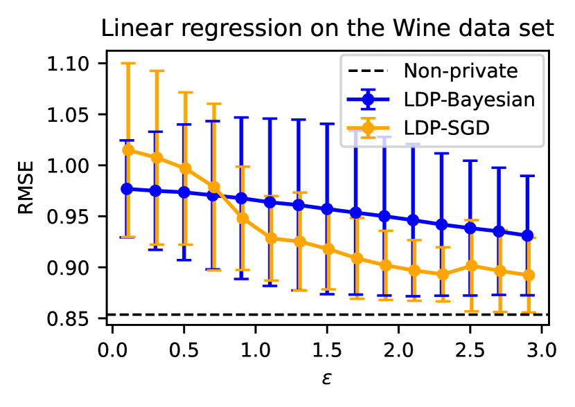
Finally, we train a linear regression model using Wine (Cortez et al.,, 2009) data that comprises of roughly 6.5K samples with 12 features. We set $R_{y}=2$. A $80/20$% train/test split was used.

4.2 Private baseline — LDP-SGD

We compare our regression models with a local version of DP-SGD adapted from Wang et al., 2019b to our case study. They make the privacy cost invariant to the number of training iterations by having each user participate only once in the training. They partition the users into the groups of size $G=\Omega(\frac{d\log(d)}{\epsilon^{2}})$. However, unlike in standard DP-SGD, the aggregator makes model updates for group $i$ only after receiving the noisy gradients from group $i-1$. The gradients are perturbed using Gaussian noise (with $\Delta_{2}=2$) after clipping their $L_{2}$ norm to 1. In total, $2N-G$ messages are exchanged in the protocol, which is roughly $2N$ for large enough $\epsilon$’s.

Pre-processing for regression tasks. To reduce the training time to be more manageable, we use principal component analysis (PCA) to reduce the original dimensionality of our data sets. Additionally, we center our data sets to zero mean.

4.3 Default settings and implementation

Both noise-aware and non-private baseline models are implemented either in Stan (Carpenter et al.,, 2017) or NumPyro (Phan et al.,, 2019; Bingham et al.,, 2018). We use No-U-Turn (Homan and Gelman,, 2014) sampler, which is a variant of Hamiltonian Monte Carlo. We run 4 Markov chains in parallel and discard the first 50% as warm-up samples. We ensure that the Gelman-Rubin convergence statistic (Brooks and Gelman,, 1998) for all models remains consistently below 1.1 for all experiments. For regression experiments, we fix $R=1$ to use Corollary 3.1 and  13.1.

Prior selection. The priors for model parameters are specified in Table 8, and in Section 8 in the Supplement. The arguments to these priors are the hyper-parameters for the model.

4.4 Uncertainty calibration

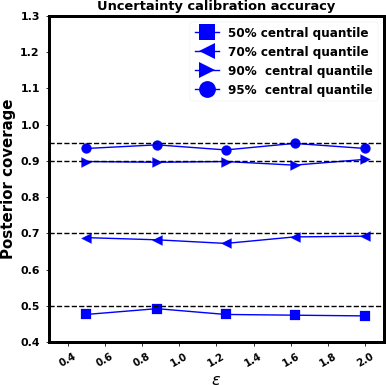
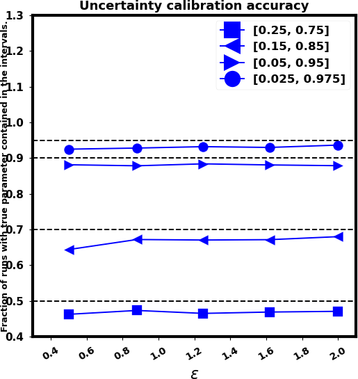
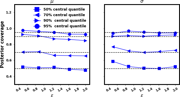
For the deployment of the learned models, it is crucial that the uncertainty estimates of the models are calibrated. Overestimation of variance would lead to uninformative posteriors whereas underestimation can lead to overconfident estimates. To assess this, we use synthetic data sampled from prior predictive distribution and learn the posterior distributions for the model parameters. We repeat this multiple times, and count the fraction of runs that included the data generating parameters for several central quantiles of the posterior samples. Figure 1 shows the posterior calibration for the Gaussian parameter estimation model as a function of $\epsilon$. We can see that our posteriors are well calibrated even for the most strict privacy constraints. The plots for the histogram and exponential distribution models can be found in Figures 10 and 11 in the supplement.

4.5 Accuracy of private posteriors

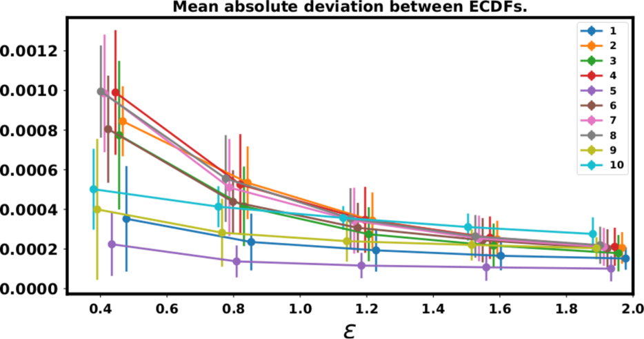
We can also test the accuracy of our model by directly comparing the private and non-private posteriors. Figure 2 compares the mean absolute deviation over 50 repeats in the empirical cumulative density function (ECDF) of the private posteriors of the multinomial probabilities from the non-private for the Kosarak data set. We verify that our private posteriors, despite adhering to LDP guarantees, are quite close to the non-private posteriors.

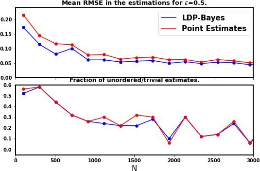
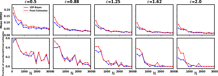
Additionally, to motivate the benefit of including the whole data generation process in a single model, we compare the posterior means of our histogram aggregation model to the private point estimates. As mentioned in Section 3.2.2, the denoised point estimates may not satisfy simplexity, especially for strong privacy parameters and/or low sample size. We can enforce simplexity in these estimates with additional post-processing e.g. by computing their least squares approximations (Hay et al.,, 2010). While the least squares solution is well principled, it is disconnected from the main LDP protocol. By modeling $\boldsymbol{\theta}$ as a multinomial distribution, we automatically satisfy $\boldsymbol{\theta}$’s simplexity in the model itself. This leads to better utility in some cases. Figure 3 compares the mean squared error in reconstruction for a three dimensional histogram with true weights $[0.7,0.2,0.1]$ for both methods for $\epsilon=0.5$. We observe that the error in our model is lower by 10-30%, specially in low sample size regimes. The comparison for more $\epsilon$ values can be found in Figure  9 in Supplement.

4.6 Accuracy of inference

Besides being able to correctly estimate the uncertainty of model parameters, we want our inference to also be accurate. Towards this goal, we compare the performance metrics of our regression models to LDP-SGD (Section 4.2).

Linear regression. We trained the linear regression model using the Wine (Cortez et al.,, 2009) data set. Figure 4 shows that the sufficient statistics based Bayesian model performs well under strict privacy guarantees. The comparison method (LDP-SGD) starts to perform better when we increase the privacy budget. As the sufficient statistic based model is trained on clipped inputs, it may underestimate the test targets which are unclipped, thus hurting the RMSE.

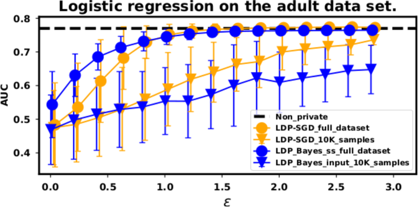
Logistic regression. We run the sufficient statistic based model for all 48K records of the adult data set. However, for the input based model (Section 3.2.3), we use randomly sampled $10K/48K$ records to reduce the training time. We choose $c=0.5$ because this split yielded the best utility in our internal experiments (not included). For a fair comparison, we also run LDP-SGD with the same 10K records.

Figure 5 compares the mean AUC for LDP-SGD, and both models for various privacy parameters. We verify that for $\epsilon\leq 0.8$, the sufficient statistics based Bayesian model outperforms DP-SGD. For large enough $\epsilon$’s, sufficient statistics based Bayesian model achieves nearly the same level of performance as DP-SGD without additional rounds of messages from aggregator. The input based model cannot, however, perform at a similar level. This is possibly caused by the large amount of noise (due to the budget split), that suppress the covariance information necessary for accurate inference. In contrast, the covariance structure is perturbed relatively cheaply in the sufficient statistics based solution due to tight privacy accounting. We exclude the input based solution from our next plot.

Figure 1: Gaussian parameter estimation: Even under strict privacy guarantees, the posteriors are well calibrated. Figure shows posterior coverage calculated from $5000$ Gaussian samples (clipped to $[-5,5]$) over 500 repeats.

Figure 2: Histogram discovery: The LDP variant performs close to non-private even in the strict privacy regime and converges to the non-private posteriors. The figure shows the mean absolute difference over 50 repeats between the empirical CDFs of private and non-private posteriors for each of the 10 dimensions of an abridged version of the Kosarak (Benson et al.,, 2018) data set.

Figure 3: Histogram estimation: The full-Bayesian version of the histogram aggregation method OUE (Wang et al.,, 2017) outperforms the corresponding point estimates for small sample sizes. Top: the mean RMSE across 50 independent runs for LDP posterior means and $L_{2}$ approximations of LDP point estimates. The true histogram parameters ([0.7,0.2,0.1]) were used as the ground truth for computing RMSE. Bottom: the fraction of unusable or misleading (trivial, unordered) solutions produced by the Bayesian and the point estimates model.

Figure 4: Linear regression: In the most important high-privacy region (small $\epsilon$) the sufficient statistics based Bayesian model outperforms the private baseline (LDP-SGD). However, as the $\epsilon$ increases the SGD based solution starts to perform better that the Bayesian approach. The results show the average test RMSE on Wine data set over 30 independent repeats of the inference and the errorbars denote the standard deviation among the repeats.

Figure 5: Logistic regression: The sufficient statistics based private logistic regression model almost matches the private and the non-private baselines as $\epsilon$ increases. The figure shows the average AUC for adult data set (Blake and Merz,, 1998) for LDP-SGD and Bayesian models based on perturbed inputs and sufficient statistics. The mean is computed over 30 independent repeats of the inference. The errorbars are slightly shifted for readability and denote the standard deviation among the repeats.

5 Discussion and concluding remarks

In this work we have initiated the study of designing noise-aware models for performing Bayesian inference under LDP. Our models are well calibrated and outperform the point estimations for small privacy/sample size regimes.

With hierarchical modeling, these approaches easily extend to other interesting scenarios for pooled analysis between different sub-populations, such as personalized privacy budgets (Chen et al.,, 2016; Jorgensen et al.,, 2015), hybrid model (Avent et al.,, 2017), and multi-party differential privacy (Vadhan,, 2017) with minor modifications. Additionally, our models maintain full compatibility with more recent amplification techniques such as shuffling (Erlingsson et al.,, 2019).

Feature sub-sampling is routinely used in LDP protocols to amplify privacy and reduce communication. The current framework does not efficiently model protocols involving sub-sampling because unsampled features in each input become the latent variables of the model, thus exploding the model complexity. The question of modeling the uncertainty due to sub-sampling is left as a future exercise.

6 Acknowledgement

This work was supported by the Academy of Finland (Flagship programme: Finnish Center for Artificial Intelligence, FCAI) Grants 325572, 325573, the Strategic Research Council at the Academy of Finland (Grant 336032) as well as UKRI Turing AI World-Leading Researcher Fellowship, EP/W002973/1. We are grateful to the Aalto Science-IT project for their computational resources.

 

Locally Differentially Private Bayesian Inference

 

7 Chebyshev approximation

The polynomial expansion can be used to approximate a non-linear function by expressing it as a sum of monomials. Among several choices, Chebyshev polynomials (Mason and Handscomb,, 2002) are often chosen because the quality of approximation is uniform over any finite interval $[-R,R],R>0$. The Chebyshev polynomial expansion of degree $M$ for the sigmoid of $\boldsymbol{x}^{T}\boldsymbol{\theta}$ is given below.

$$\frac{\exp(\boldsymbol{x}^{T}\boldsymbol{\theta})}{1+\exp(\boldsymbol{x}^{T}\boldsymbol{\theta})}\approx\sum_{m=0}^{M}b_{m}(\boldsymbol{x}^{T}\boldsymbol{\theta})^{m}=\sum_{m=0}^{M}b_{m}\sum_{\boldsymbol{e}\in\mathbb{N}^{d}:\sum_{j}\boldsymbol{e}_{j}=m}{m\choose\boldsymbol{e}}(\boldsymbol{\theta})^{\boldsymbol{e}}(\boldsymbol{x})^{\boldsymbol{e}}.$$ (12)

In the above expression, $(\boldsymbol{x})^{\boldsymbol{e}}=\prod_{j\in[d]}x_{j}^{e_{j}},\boldsymbol{x}\in\mathbb{R}^{d},\boldsymbol{e}\in\mathbb{N}^{d}$. ${m\choose\boldsymbol{e}}=\frac{m!}{\prod_{j=1}^{d}e_{j}!}$ are the multinomial coefficients. The constants $b_{0},b_{1},\cdots,b_{M}$ are the Chebyshev coefficients computed over an arbitrary finite interval. In general, $M$ order approximation contains ${d+M\choose d}$ summands. Figure 7 shows a 2nd order expansion of the sigmoid function.

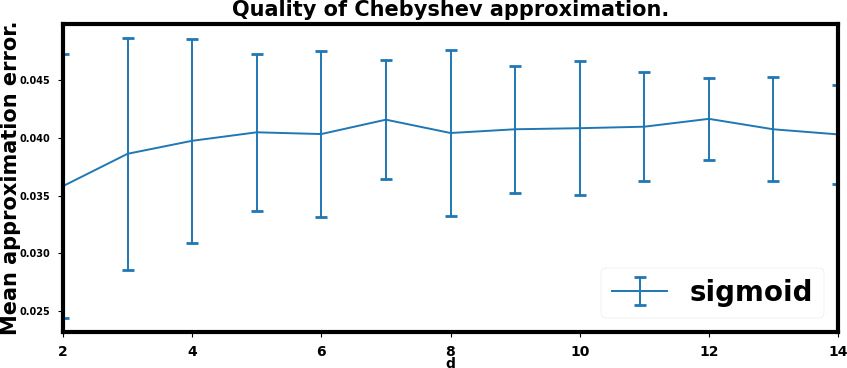
Quality of approximation. We would like to empirically understand the quality of approximation for the expression $\mathbb{E}_{x\sim\mathcal{N}^{d}(\boldsymbol{0},\boldsymbol{\Sigma})}(\frac{\exp(\boldsymbol{x}^{T}\boldsymbol{\theta})}{1+\exp(\boldsymbol{x}^{T}\boldsymbol{\theta})})$, for a fixed $\boldsymbol{\theta}\in\mathbb{R}^{d}$ and $\boldsymbol{\Sigma}\in\mathbb{R}^{d\times d}$.

Figure 6: We plot the mean absolute difference between empirical expectation of sigmoid($\boldsymbol{x}^{T}\boldsymbol{\theta}$) and its 2nd order Chebyshev approximation with $b_{0},b_{1},b_{2}\in[-3,3]$. The mean absolute deviation is computed over 50 independent runs. In each run, we sample a new $\boldsymbol{\theta}$ from standard normal distribution, and the empirical expectation is taken over $1000$ samples drawn from a zero centered multivariate Gaussian with a random full rank co-variance matrix. The co-variance matrix remains fixed for a given dimension for all runs. We also restrict the $L_{2}$ norm of these samples to 1. We can observe that the approximation is moderately accurate.

$\sigma(\boldsymbol{x}^{T}\boldsymbol{\theta})\approx b_{0}+b_{1}x_{1}\theta_{1}+b_{1}x_{2}\theta_{2}+b_{1}x_{3}\theta_{3}+b_{2}x_{1}^{2}\theta^{2}_{1}+b_{2}x_{2}^{2}\theta^{2}_{2}+b_{2}x_{3}^{2}\theta^{2}_{3}+2b_{2}x_{1}x_{2}\theta_{1}\theta_{2}+2b_{2}x_{1}x_{3}\theta_{1}\theta_{3}+2b_{2}x_{2}x_{3}\theta_{2}\theta_{3}$

Figure 7: An example of 2nd order Chebyshev expansion of the sigmoid function for $\boldsymbol{x},\boldsymbol{\theta}\in\mathbb{R}^{3}$.

8 Priors for probabilistic models

Model	Prior
Gaussian	$\theta\sim\mathcal{N}(\mu_{0},\sigma_{0})$ and $\sigma\sim$ Gamma$(\alpha,\beta)$
Exponential	$\theta\sim$ Gamma$(\alpha,\beta)$
Multinomial	$\boldsymbol{\theta}\sim$Dirichlet($\{1\}^{d}$)
Regression	$\boldsymbol{\theta}\sim\mathcal{N}(0,5\boldsymbol{I})$), $\boldsymbol{\Sigma}\sim$ scaled LKJ prior

Figure 8: Priors

LKJ prior for $\boldsymbol{\Sigma}$ (Lewandowski et al.,, 2009). We scale a positive definite correlation matrix from the LKJ correlation distribution of shape $\eta=2$ from both sides with a diagonal matrix with $\mathcal{N}(0,2.5)$ distributed diagonal entries. The probabilistic model is:

$$\boldsymbol{\Omega} \sim\text{LKJ}(2),\quad\boldsymbol{\tau}\sim\mathcal{N}(\mathbf{0},2.5\cdot\mathbf{I}),$$

$$\boldsymbol{\Sigma} =\text{diag}(\boldsymbol{\tau})\,\Omega\,\text{diag}(\boldsymbol{\tau}).$$

9 Missing Proofs

9.1 Proof of Lemma 3.1

Proof.

Let $\{\boldsymbol{x},y\},\{\boldsymbol{x}^{\prime},y^{\prime}\}$ be the neighboring input pairs. We assume that $||\boldsymbol{x}||_{2}\leq R,||\boldsymbol{x}^{\prime}||_{2}\leq R,|y|,|y^{\prime}|\leq R_{y}$. The Gaussian mechanism $\mathcal{M}$ for a single input $\{\boldsymbol{x},y\}$ is,

$$\mathcal{M}(\boldsymbol{x}) \sim\begin{bmatrix}\boldsymbol{t}_{2}(\boldsymbol{x})\\ y\boldsymbol{t}_{1}(\boldsymbol{x})\\ y^{2}\end{bmatrix}+\mathcal{N}\left(0,\begin{bmatrix}\sigma_{1}^{2}\boldsymbol{I}_{d_{2}}&0&0\\ 0&\sigma_{2}^{2}\boldsymbol{I}_{d}&0\\ 0&0&\sigma_{3}^{2}\\ \end{bmatrix}\right)$$ (13)

$$\mathcal{M}(\boldsymbol{x}) \sim\begin{bmatrix}\boldsymbol{I}_{d}&0&0\\ 0&\frac{\sigma_{2}}{\sigma_{1}}\boldsymbol{I}_{d_{2}}&0\\ 0&0&\frac{\sigma_{3}}{\sigma_{1}}\\ \end{bmatrix}\left(\begin{bmatrix}\boldsymbol{t}_{2}(\boldsymbol{x})\\ \frac{\sigma_{1}}{\sigma_{2}}y\boldsymbol{t}_{1}(\boldsymbol{x})\\ \frac{\sigma_{1}}{\sigma_{3}}y^{2}\end{bmatrix}+\mathcal{N}(0,\sigma_{1}^{2}\boldsymbol{I}_{d_{2}+d+1})\right).$$

Removing the constant scaling, we see that it is equivalent to the following mechanism.

$$\mathcal{M}(\boldsymbol{x})=\begin{bmatrix}\boldsymbol{t}_{2}(\boldsymbol{x})\\ \frac{\sigma_{1}}{\sigma_{2}}y\boldsymbol{t}_{1}(\boldsymbol{x})\\ \frac{\sigma_{1}}{\sigma_{3}}y^{2}\end{bmatrix}+\mathcal{N}(0,\sigma_{1}^{2}\boldsymbol{I}_{d_{2}+d+1}).$$

Define

$$F(\boldsymbol{x},y)=\begin{bmatrix}\boldsymbol{t}_{2}(\boldsymbol{x})\\ \frac{\sigma_{1}}{\sigma_{2}}y\boldsymbol{t}_{1}(\boldsymbol{x})\\ \frac{\sigma_{1}}{\sigma_{3}}y^{2}\end{bmatrix}.$$

For the first order terms,

$$||y\boldsymbol{t}_{1}(\boldsymbol{x})-y^{\prime}\boldsymbol{t}_{1}(\boldsymbol{x}^{\prime})||^{2}_{2} =\sum_{j}(yx_{j}-y^{\prime}x^{\prime}_{j})^{2}=y^{2}\sum_{j}x^{2}_{j}+y^{\prime 2}\sum_{j}x^{\prime 2}_{j}-2yy^{\prime}\sum_{j}x_{j}x^{\prime}_{j}$$ (14)

$$\leq 2R^{2}_{y}R^{2}-2yy^{\prime}\langle\boldsymbol{x},\boldsymbol{x}^{\prime}\rangle.$$

Similarly, $(y^{2}-y^{\prime 2})^{2}\leq R_{y}^{4}$. For the second order terms,

$$\norm{\boldsymbol{t}_{2}(\boldsymbol{x})-\boldsymbol{t}_{2}(\boldsymbol{x}^{\prime})}_{2}^{2} =\sum\limits_{j}(x_{j}^{2}-x_{j}^{\prime 2})^{2}+2\sum\limits_{j>k}(x_{j}x_{k}-x_{j}^{\prime}x_{k}^{\prime})^{2}$$ (15)

$$=\sum\limits_{j}x_{j}^{4}+\sum\limits_{j}x_{j}^{\prime 4}-2\sum\limits_{j}x_{j}^{2}x_{j}^{\prime 2}+2\sum\limits_{j>k}x_{j}^{2}x_{k}^{2}+2\sum\limits_{j>k}x_{j}^{\prime 2}x_{k}^{\prime 2}-4\sum\limits_{j>k}x_{j}x_{k}x_{j}^{\prime}x_{k}^{\prime}$$

$$=\left(\sum\limits_{j}x_{j}^{4}+2\sum\limits_{j>k}x_{j}^{2}x_{k}^{2}\right)+\left(\sum\limits_{j}x_{j}^{\prime 4}+2\sum\limits_{j>k}x_{j}^{\prime 2}x_{k}^{\prime 2}\right)-2\sum\limits_{j}x_{j}^{2}x_{j}^{\prime 2}-4\sum\limits_{j>k}x_{j}x_{k}x_{j}^{\prime}x_{k}^{\prime}$$

$$=\left(\sum\limits_{j}x_{j}^{4}+\sum\limits_{j\neq k}x_{j}^{2}x_{k}^{2}\right)+\left(\sum\limits_{j}x_{j}^{\prime 4}+\sum\limits_{j\neq k}x_{j}^{\prime 2}x_{k}^{\prime 2}\right)-2\sum\limits_{j}x_{j}^{2}x_{j}^{\prime 2}-2\sum\limits_{j\neq k}x_{j}x_{k}x_{j}^{\prime}x_{k}^{\prime}$$

$$=\norm{\boldsymbol{x}}_{2}^{4}+\norm{\boldsymbol{x}^{\prime}}_{2}^{4}-2\langle\boldsymbol{x},\boldsymbol{x}^{\prime}\rangle^{2}\leq 2R^{4}-2\langle\boldsymbol{x},\boldsymbol{x}^{\prime}\rangle^{2}.$$

Finally,

$$\norm{F(\boldsymbol{x},y)-F(\boldsymbol{x}^{\prime},y^{\prime})}^{2}_{2} =\norm{\boldsymbol{t}_{2}(\boldsymbol{x})-\boldsymbol{t}_{2}(\boldsymbol{x}^{\prime})}^{2}_{2}+\frac{\sigma_{1}^{2}}{\sigma_{2}^{2}}\norm{y\boldsymbol{t}_{1}(\boldsymbol{x})-y^{\prime}\boldsymbol{t}_{1}(\boldsymbol{x}^{\prime})}^{2}_{2}+\frac{\sigma_{1}^{2}}{\sigma_{3}^{2}}(y^{2}-y^{\prime 2})^{2}$$ (16)

$$\leq 2R^{4}-2\langle\boldsymbol{x},\boldsymbol{x}^{\prime}\rangle^{2}+\frac{\sigma_{1}^{2}}{\sigma_{2}^{2}}[2R_{y}^{2}R^{2}-2yy^{\prime}\langle\boldsymbol{x},\boldsymbol{x}^{\prime}\rangle]+\frac{\sigma_{1}^{2}}{\sigma_{3}^{2}}R_{y}^{4}$$

$$=2R^{4}-2t^{2}+2c_{1}R_{y}^{2}R^{2}-2c_{1}yy^{\prime}t+c_{2}R_{y}^{4},$$

where $c_{1}=\frac{\sigma_{1}^{2}}{\sigma_{2}^{2}}$, $c_{2}=\frac{\sigma_{1}^{2}}{\sigma_{3}^{2}}$ and $t=\langle\boldsymbol{x},\boldsymbol{x}^{\prime}\big{\rangle}$. Above quadratic equation maximizes at $t=-\frac{c_{1}yy^{\prime}}{2}=-\frac{c_{1}R_{y}^{2}}{2}$ and the maximum value is,

$$\Delta_{2}(\boldsymbol{t})=\norm{F(\boldsymbol{x},y)-F(\boldsymbol{x}^{\prime},y^{\prime})}_{2}\leq\sqrt{\frac{\sigma_{1}^{4}R_{y}^{4}}{2\sigma_{2}^{4}}+2R^{4}+\frac{2\sigma_{1}^{2}R_{y}^{2}R^{2}}{\sigma_{2}^{2}}+\frac{\sigma_{1}^{2}R_{y}^{4}}{\sigma_{3}^{2}}}.$$ (17)

∎

9.2 Proof of Lemma 3.2

Proof.

Let us write $g(x)=\sum_{j=0}^{M}g_{j}x^{j}$ and $h(x)=\sum_{i=0}^{2}h_{i}x^{i}$. Now the integral in (7) becomes

$$\Pr[z]=\int_{a}^{b}\Pr[z\mid x]\Pr[x]\differential x=C\frac{1}{\sqrt{2\pi\sigma^{2}}}\sum_{j=0}^{M}g_{j}\int_{a}^{b}x^{j}\exp{-\frac{1}{2\sigma^{2}}\left[(z-x)^{2}-\sum_{i=0}^{2}h_{i}x^{i}\right]}\differential x.$$ (18)

We can clearly see that the exponential term inside the integral is yet another Gaussian kernel of $x$. Next we write the polynomial inside the exponential in a quadratic form:

$$(z-x)^{2}-\sum_{i=0}^{2}h_{i}x^{i} =(1-h_{2})x^{2}-2(z+\frac{h_{1}}{2})x+z^{2}-h_{0}$$ (19)

$$=(1-h_{2})\left[x^{2}-2\frac{(z+\frac{h_{1}}{2})}{(1-h_{2})}x+\frac{(z+\frac{h_{1}}{2})^{2}}{(1-h_{2})^{2}}-\frac{(z+\frac{h_{1}}{2})^{2}}{(1-h_{2})^{2}}\right]+z^{2}-h_{0}$$

$$=(1-h_{2})\left(x-\frac{z+\frac{h_{1}}{2}}{1-h_{2}}\right)^{2}+z^{2}-h_{0}-\frac{(z+\frac{h_{1}}{2})^{2}}{1-h_{2}}.$$

Denote $s^{2}=\frac{\sigma^{2}}{1-h_{2}}$ and $m=\frac{2z+h_{1}}{2-2h_{2}}$, we get

$$\Pr[z]=C\frac{1}{\sqrt{2\pi\sigma^{2}}}\sqrt{2\pi s^{2}}\sum_{j=0}^{M}g_{j}\int_{a}^{b}x^{j}\mathcal{N}(x;m,s^{2})\exp(-\frac{1}{2\sigma^{2}}\left(z^{2}-h_{0}-\frac{(z+\frac{h_{1}}{2})^{2}}{1-h_{2}}\right))\differential x,$$ (20)

where $\mathcal{N}(\cdot;m,s^{2})$ denotes the probability density function of a Gaussian with mean $m$ and variance $s^{2}$. Now, after removing the constant factors out of the integral, we are left with integral

$$\int_{a}^{b}x^{j}\mathcal{N}(x;m,s^{2})\differential x=\left(\Phi\left(\frac{b-m}{s}\right)-\Phi\left(\frac{a-m}{s}\right)\right)\mathbb{E}_{x\sim\text{TrunNorm(m,s,a,b)}}[x^{j}],$$ (21)

where $\Phi$ is the cumulative density function of a std. normal distribution. Now in order to conclude the proof, it suffices to show that the truncated normal distribution has the non-central moments in an tractable form, which has been shown in the past for example by Flecher et al., (2010). ∎

10 Likelihood calculations — uni-variate parameter estimations.

We denote $\Phi_{\boldsymbol{\theta}}(a)=\Pr[x\leq a]$ as the cumulative density function of the corresponding density function.

10.1 Gaussian distribution

We assume the distribution is rectified from both sides with $(a,b)$ and data points are perturbed with $\epsilon$-DP Laplace noise. We intend to learn both mean $\mu$ and variance $\sigma^{2}$. Let $\boldsymbol{\theta}=[\mu,\sigma]$).

$$\Pr[z\mid\boldsymbol{\theta}] =\int_{\mathbb{R}}\Pr[z,x\mid\boldsymbol{\theta}]dx=\int_{\mathbb{R}}\Pr[z\mid x]\times\Pr[x\mid\boldsymbol{\theta},a,b]dx$$ (22)

$$=\frac{\epsilon}{2(b-a)}\int_{\mathbb{R}}\exp(-\frac{\epsilon|z-x|}{(b-a)})\Pr[x\mid\boldsymbol{\theta},a,b]dx$$ (23)

$$=\frac{\epsilon}{2(b-a)}\int_{\mathbb{R}}\exp(-\frac{\epsilon|z-x|}{b-a})\Big{[}\delta_{a}(x)\Phi_{\boldsymbol{\theta}}(a)+\mathbf{1}_{(a<x<b)}\Phi_{\boldsymbol{\theta}}(x)+\delta_{b}(x)(1-\Phi_{\boldsymbol{\theta}}(b))\Big{]}dx$$ (24)

$$=\frac{\epsilon\Phi_{\boldsymbol{\theta}}(a)}{2(b-a)}\exp(-\frac{\epsilon|z-a|}{b-a})+\frac{\epsilon(1-\Phi_{\boldsymbol{\theta}}(b))}{2(b-a)}\exp(-\frac{\epsilon|z-b|}{b-a})$$ (25)

$$+\frac{\epsilon}{2\sqrt{2\pi}(b-a)\sigma}\int_{a}^{b}\exp(-\frac{\epsilon|z-x|}{b-a})\exp(-\frac{(x-\mu)^{2}}{2\sigma^{2}})dx.$$ (26)

Now we focus on the integral in step 26. Since $x\in[a,b]$ and $z\in\mathbb{R}$, the sign of the term $|z-x|$ depends on $z$. To simplify, we set limit $l=max(a,min(b,z))$.

$$\int_{a}^{b}\exp(\frac{-\epsilon|x-z|}{(b-a)})\exp(-\frac{(x-\mu)^{2}}{2\sigma^{2}})dx$$ (27)

$$=\int_{a}^{l}\exp(\frac{\epsilon(x-z)}{b-a})\exp(-\frac{(x-\mu)^{2}}{2\sigma^{2}})dx+\int_{l}^{b}\exp(\frac{\epsilon(z-x)}{b-a})\exp(-\frac{(x-\mu)^{2}}{2\sigma^{2}})dx$$

$$=-\dfrac{\sqrt{{\pi}}{\sigma}\left(\operatorname{erf}\left(\frac{{\epsilon}{\sigma}^{2}+\left(b-a\right)\left({\mu}-l\right)}{\sqrt{2}\left(b-a\right){\sigma}}\right)-\operatorname{erf}\left(\frac{{\epsilon}{\sigma}^{2}+\left(b-a\right)\left({\mu}-a\right)}{\sqrt{2}\left(b-a\right){\sigma}}\right)\right)\exp(-\frac{{\epsilon}\left(2\left(b-a\right)\left(z-{\mu}\right)-{\epsilon}{\sigma}^{2}\right)}{2\left(b-a\right)^{2}})}{\sqrt{2}}$$

$$-\dfrac{\sqrt{{\pi}}{\sigma}\left(\operatorname{erf}\left(\frac{{\epsilon}{\sigma}^{2}-\left(b-a\right)\left({\mu}-l\right)}{\sqrt{2}\left(b-a\right){\sigma}}\right)-\operatorname{erf}\left(\frac{{\epsilon}{\sigma}^{2}-\left(b-a\right)\left({\mu}-b\right)}{\sqrt{2}\left(b-a\right){\sigma}}\right)\right)\mathrm{e}^{\frac{{\epsilon}\left(2\left(b-a\right)\left(z-{\mu}\right)+{\epsilon}{\sigma}^{2}\right)}{2\left(b-a\right)^{2}}}}{\sqrt{2}}$$

Putting this all together yields

$$\Pr[z\mid\boldsymbol{\theta}]= \frac{\epsilon\Phi_{\boldsymbol{\theta}}(a)}{2(b-a)}\exp(-\frac{\epsilon|z-a|}{b-a})+\frac{\epsilon(1-\Phi_{\boldsymbol{\theta}}(b))}{2(b-a)}\exp(-\frac{\epsilon|z-b|}{b-a})$$ (28)

$$+\frac{\epsilon}{4(b-a)}\mathrm{e}^{\frac{(\epsilon\sigma)^{2}}{2(b-a)^{2}}}\Bigg{(}\left(\operatorname{erf}\left(\frac{{\epsilon}{\sigma}^{2}+\left(b-a\right)\left({\mu}-a\right)}{\sqrt{2}\left(b-a\right){\sigma}}\right)-\operatorname{erf}\left(\frac{{\epsilon}{\sigma}^{2}+\left(b-a\right)\left({\mu}-l\right)}{\sqrt{2}\left(b-a\right){\sigma}}\right)\right)\exp(-\frac{{\epsilon}\left(z-{\mu}\right)}{(b-a)})$$

$$+\left(\operatorname{erf}\left(\frac{{\epsilon}{\sigma}^{2}-\left(b-a\right)\left({\mu}-b\right)}{\sqrt{2}\left(b-a\right){\sigma}}\right)-\operatorname{erf}\left(\frac{{\epsilon}{\sigma}^{2}-\left(b-a\right)\left({\mu}-l\right)}{\sqrt{2}\left(b-a\right){\sigma}}\right)\right)\exp(\frac{{\epsilon}\left(z-{\mu}\right)}{(b-a)})\Bigg{)}$$

10.2 Exponential distribution

$$\Pr[z\mid\theta,b] =\int_{0}^{\infty}\Pr[z,x|\theta,b]dx=\int_{0}^{\infty}\Pr[z|x]\times\Pr[x|\theta,b]dx$$ (29)

$$=\int_{0}^{\infty}\frac{\epsilon}{2b}\exp(\frac{-\epsilon|z-x|}{b})\Big{[}\mathbf{1}_{(x\leq b)}f(x)+\delta_{b}(x)(1-\Phi_{\theta}(b))\Big{]}dx$$

$$=\frac{\epsilon}{2b}\Big{[}\int_{0}^{\infty}\exp(\frac{-\epsilon|z-x|}{b})\theta\exp(-\theta x)dx+\int_{0}^{\infty}\exp(\frac{-\epsilon|z-x|}{b})\exp(-\theta b)\delta_{b}(x)dx\Big{]}$$

Let us workout the first integration for the first case. The sign of $|z-x|$ may switch if $z<0$ and it may affect the outcome of the integral. So let’s set the upper limit to a temporary limit $l$. We set $l=max(0,min(b,z))$ to bound $z$ in $[0,b]$.

$$\int_{0}^{b}\exp(\frac{-|z-x|}{b/\epsilon})\theta\exp(-\theta x)dx=\int_{0}^{l}\exp(\frac{x-z}{b/\epsilon})\theta\exp(-\theta x)dx+\int_{l}^{b}\exp(\frac{z-x}{b/\epsilon})\theta\exp(-\theta x)dx$$ (30)

$$=\dfrac{b\theta\left(\exp(l\theta)-\exp(\frac{l\epsilon}{b})\right)\exp(-\frac{\epsilon z}{b}-l\theta)}{b\theta-\epsilon}+\dfrac{b\theta\left(\exp(b\theta+\epsilon)-\exp(l\theta+\frac{l\epsilon}{b})\right)\exp(\frac{\epsilon y-l\epsilon}{b}-b\theta-l\theta-\epsilon)}{b\theta+\epsilon}$$

11 Likelihood calculations for optimal unary encoding (OUE)

$$\Pr[\boldsymbol{z},x=k\mid\boldsymbol{\theta}] =\Pr[\boldsymbol{z}\mid x=k]\Pr[x=k|\boldsymbol{\theta}]$$ (31)

$$=\theta_{k}\times q^{\boldsymbol{z}_{k}}(1-q)^{1-z_{k}}\prod_{j\neq k}p^{1-z_{j}}(1-p)^{z_{j}}$$

$$=\theta_{k}\times\left(\frac{1}{2}\right)^{z_{k}}\left(1-\frac{1}{2}\right)^{1-z_{k}}p^{\sum_{j\neq k}(1-z_{j})}(1-p)^{\sum_{j\neq k}z_{j}}$$

Divide and multiply by $p^{1-z_{k}}(1-p)^{z_{k}}$.

$$\Pr[\boldsymbol{z},x=k\mid\boldsymbol{\theta}]=\theta_{k}\frac{p^{d-\sum_{j}z_{j}}(1-p)^{\sum_{j}z_{j}}}{2p^{1-z_{k}}(1-p)^{z_{k}}}$$ (32)

Let us marginalize the input $x$ out by summing over the domain.

$$\Pr[\boldsymbol{z}\mid\boldsymbol{\theta}] =\sum_{k=1}^{d}\Pr[\boldsymbol{z},x=k\mid\theta]$$ (33)

$$=p^{d-\sum_{j}z_{j}}(1-p)^{\sum_{j}z_{j}}\sum_{k=1}^{d}\frac{\theta_{k}}{2p^{1-z_{k}}(1-p)^{z_{k}}}$$

$$=p^{d}\left(\frac{1-p}{p}\right)^{\sum_{j}z_{j}}\sum_{k=1}^{d}\frac{\theta_{k}}{2p}\left(\frac{1-p}{p}\right)^{-z_{k}}$$

$$=p^{d}\exp(-\epsilon\sum_{j}z_{j})\sum_{k=1}^{d}\frac{\theta_{k}\exp(z_{k}\epsilon)}{2p}$$

The last equality is due to the fact that $\frac{1-p}{p}=\exp(-\epsilon)$.

12 Likelihood calculations for linear/logistic regression — perturbed inputs

Both models do not take any stand on how the sensitivity of the Gaussian mechanism was computed, or the way total privacy budget is split while perturbing $\boldsymbol{x}$ and y.

12.1 Linear regression

Consider the following model where we observe data through Gaussian perturbation.

$$\boldsymbol{x} \sim\mathcal{N}(\mathbf{0},\boldsymbol{\Sigma})$$ (34)

$$\boldsymbol{z}_{\boldsymbol{x}}\mid\boldsymbol{x} \sim\mathcal{N}(\boldsymbol{x},\boldsymbol{\Sigma}_{*})$$

$$y \sim\mathcal{N}(\boldsymbol{\theta}^{T}\boldsymbol{x},\sigma^{2})$$

$$z_{y}\mid y \sim\mathcal{N}(y,\sigma_{*}^{2}).$$

Next we show how to marginalize the latent inputs out from the model. We start by moving the $\boldsymbol{z}_{\boldsymbol{x}}$ out from the integral

$$\Pr[\boldsymbol{z}_{\boldsymbol{x}},z_{y}] =\int\int\Pr[\boldsymbol{x},\boldsymbol{z}_{\boldsymbol{x}}]\Pr[z_{y},y\mid\boldsymbol{x}]\differential\boldsymbol{x}\differential y$$ (35)

$$=\mathcal{N}(\boldsymbol{z}_{\boldsymbol{x}};\boldsymbol{0},\boldsymbol{\Sigma}+\boldsymbol{\Sigma}_{*})\int\int\Pr[\boldsymbol{x}\mid\boldsymbol{z}_{\boldsymbol{x}}]\Pr[y\mid\boldsymbol{x}]\Pr[\boldsymbol{z}_{y}\mid y]\differential\boldsymbol{x}\differential y$$ (36)

$$=\mathcal{N}(\boldsymbol{z}_{\boldsymbol{x}};\boldsymbol{0},\boldsymbol{\Sigma}+\boldsymbol{\Sigma}_{*})\int\Pr[\boldsymbol{z}_{y}\mid y]\int\mathcal{N}(\boldsymbol{x};\underbrace{\boldsymbol{\Sigma}(\boldsymbol{\Sigma}+\boldsymbol{\Sigma}_{*})^{-1}\boldsymbol{z}_{\boldsymbol{x}}}_{:=\boldsymbol{h}_{\boldsymbol{x}}},\underbrace{\boldsymbol{\Sigma}-\boldsymbol{\Sigma}(\boldsymbol{\Sigma}+\boldsymbol{\Sigma}_{*})^{-1}\boldsymbol{\Sigma}}_{:=\boldsymbol{A}})\Pr[y\mid\boldsymbol{x}]\differential\boldsymbol{x}\differential y.$$ (37)

Now note that since the $y$ depends on $\boldsymbol{x}$ through $\boldsymbol{\theta}^{T}\boldsymbol{x}$, the innermost integral can be written in terms of $\boldsymbol{\theta}^{T}\boldsymbol{x}$, which in turn follows a Gaussian distribution $\mathcal{N}(\boldsymbol{\theta}^{T}h_{\boldsymbol{x}},\boldsymbol{\theta}^{T}\boldsymbol{A}\boldsymbol{\theta})$:

$$\int\mathcal{N}(\boldsymbol{x};\boldsymbol{h}_{\boldsymbol{x}},\boldsymbol{A})\Pr[(y\mid\boldsymbol{x}]\differential\boldsymbol{x}=\mathbb{E}_{\boldsymbol{x}\mid\boldsymbol{z}_{\boldsymbol{x}}\sim\mathcal{N}(\boldsymbol{h}_{\boldsymbol{x}},\boldsymbol{A})}[\mathcal{N}(y;\boldsymbol{\theta}^{T}\boldsymbol{x},\sigma^{2})] =\mathbb{E}_{\boldsymbol{\theta}^{T}\boldsymbol{x}\mid\boldsymbol{z}_{\boldsymbol{x}}\sim\mathcal{N}(\boldsymbol{\theta}^{T}h_{\boldsymbol{x}},\boldsymbol{\theta}^{T}\boldsymbol{A}\boldsymbol{\theta})}[\mathcal{N}(y;\boldsymbol{\theta}^{T}\boldsymbol{x},\sigma^{2})]$$ (38)

$$=\mathcal{N}(y;\boldsymbol{\theta}^{T}\boldsymbol{h}_{\boldsymbol{x}},\boldsymbol{\theta}^{T}\boldsymbol{A}\boldsymbol{\theta}+\sigma^{2}).$$ (39)

Finally, we substitute above into (37) and recover

$$\Pr[\boldsymbol{z}_{\boldsymbol{x}},z_{y}] =\mathcal{N}(\boldsymbol{z}_{\boldsymbol{x}};\boldsymbol{0},\boldsymbol{\Sigma}+\boldsymbol{\Sigma}_{*})\int\Pr[\boldsymbol{z}_{y}\mid y]\mathcal{N}(y;\boldsymbol{\theta}^{T}h_{\boldsymbol{x}},\boldsymbol{\theta}^{T}\boldsymbol{A}\boldsymbol{\theta}+\sigma^{2})\differential y$$ (40)

$$=\mathcal{N}(\boldsymbol{z}_{\boldsymbol{x}};\boldsymbol{0},\boldsymbol{\Sigma}+\boldsymbol{\Sigma}_{*})\mathcal{N}(\boldsymbol{z}_{y};\boldsymbol{\theta}^{T}\boldsymbol{h}_{\boldsymbol{x}},\boldsymbol{\theta}^{T}\boldsymbol{A}\boldsymbol{\theta}+\sigma^{2}+\sigma_{*}^{2}).$$ (41)

12.2 Logistic regression

Consider the following model where we observe data through Gaussian and randomized response perturbation.

$$\boldsymbol{x} \sim\mathcal{N}(\mathbf{0},\boldsymbol{\Sigma})$$ (42)

$$\boldsymbol{z}_{\boldsymbol{x}}\mid\boldsymbol{x} \sim\mathcal{N}(\boldsymbol{x},\boldsymbol{\Sigma}_{*})$$

$$y \sim\mathbb{Bern}\Big{(}\frac{1}{1+\exp(-\boldsymbol{x}^{T}\boldsymbol{\theta})}\Big{)}$$

$$z_{y}\mid y \sim\mathbb{Bern}(p).$$

Next we show how to marginalize the latent inputs out from the model. Using the property A5 from (Särkkä,, 2013), we have

$$\boldsymbol{z}_{\boldsymbol{x}} \sim\mathcal{N}(\mathbf{0},\boldsymbol{\Sigma}_{*}+\boldsymbol{\Sigma})$$

$$\boldsymbol{x}\mid\boldsymbol{z}_{\boldsymbol{x}} \sim\mathcal{N}(\boldsymbol{\Sigma}(\boldsymbol{\Sigma}+\boldsymbol{\Sigma}_{*})^{-1}\boldsymbol{z}_{\boldsymbol{x}},\boldsymbol{\Sigma}-\boldsymbol{\Sigma}(\boldsymbol{\Sigma}+\boldsymbol{\Sigma}_{*})^{-1}\boldsymbol{\Sigma}).$$

We denote the posterior parameters with $\mathbf{h}=\boldsymbol{\Sigma}(\boldsymbol{\Sigma}+\boldsymbol{\Sigma}_{*})^{-1}\boldsymbol{z}_{\boldsymbol{x}}$ and $\boldsymbol{A}=\boldsymbol{\Sigma}-\boldsymbol{\Sigma}(\boldsymbol{\Sigma}+\boldsymbol{\Sigma}_{*})^{-1}\boldsymbol{\Sigma}$. Now we can write

$$\Pr[\boldsymbol{z}_{\boldsymbol{x}},z_{y}|\boldsymbol{\theta},\boldsymbol{\Sigma}] =\int_{\Omega(\boldsymbol{X})\Omega(\boldsymbol{Y})}\Pr[\boldsymbol{z}_{\boldsymbol{x}},z_{y},\boldsymbol{x},y|\boldsymbol{\theta},\boldsymbol{\Sigma}]d\Omega(\boldsymbol{X})d\Omega(\boldsymbol{Y})$$ (43)

$$=\int_{\Omega(\boldsymbol{X})\Omega(\boldsymbol{Y})}\Pr[\boldsymbol{x}|\boldsymbol{z}_{\boldsymbol{x}},\boldsymbol{\Sigma}]\Pr[z_{y}|y]\Pr[y|\boldsymbol{x},\boldsymbol{\theta}]\Pr[\boldsymbol{z}_{\boldsymbol{x}}|\boldsymbol{\Sigma}]d\Omega(\boldsymbol{X})d\Omega(\boldsymbol{Y})$$

$$=\Pr[\boldsymbol{z}_{\boldsymbol{x}}\mid\boldsymbol{\Sigma}]\int_{\Omega(\boldsymbol{X})\Omega(\boldsymbol{Y})}\Pr[\boldsymbol{x}|\boldsymbol{z}_{\boldsymbol{x}},\boldsymbol{\Sigma}]\Pr[z_{y}|y]\Pr[y|\boldsymbol{x},\boldsymbol{\theta}]d\Omega(\boldsymbol{X})d\Omega(\boldsymbol{Y})$$

$$=\Pr[\boldsymbol{z}_{\boldsymbol{x}}\mid\boldsymbol{\Sigma}]\int_{\Omega(\boldsymbol{X})}\Pr[\boldsymbol{x}|\boldsymbol{z}_{\boldsymbol{x}},\boldsymbol{\Sigma}]\sum_{j\in\{1,0\}}p^{\mathbf{1}_{j=z_{y}}}(1-p)^{\mathbf{1}_{j\neq z_{y}}}\Pr[y=j|\boldsymbol{x},\boldsymbol{\theta}]d\Omega(\boldsymbol{X})$$

$$=\Pr[\boldsymbol{z}_{\boldsymbol{x}}\mid\boldsymbol{\Sigma}]\int_{\Omega(\boldsymbol{X})}\Pr[\boldsymbol{x}|\boldsymbol{z}_{\boldsymbol{x}},\boldsymbol{\Sigma}]\sum_{j\in\{1,0\}}p^{\mathbf{1}_{j=z_{y}}}(1-p)^{\mathbf{1}_{j\neq z_{y}}}\sigma(\boldsymbol{x}^{T}\boldsymbol{\theta})^{j}(1-\sigma(\boldsymbol{x}^{T}\boldsymbol{\theta}))^{1-j}d\Omega(\boldsymbol{X})$$

$$=\Pr[\boldsymbol{z}_{\boldsymbol{x}}\mid\boldsymbol{\Sigma}]\int_{\Omega(\boldsymbol{X})}\Pr[\boldsymbol{x}|\boldsymbol{z}_{\boldsymbol{x}},\boldsymbol{\Sigma}]\sum_{j\in\{1,0\}}(\frac{p}{1-p})^{\mathbf{1}_{j=z_{y}}}(1-p)\Big{(}\frac{\sigma(\boldsymbol{x}^{T}\boldsymbol{\theta})}{1-\sigma(\boldsymbol{x}^{T}\boldsymbol{\theta})}\Big{)}^{j}(1-\sigma(\boldsymbol{x}^{T}\boldsymbol{\theta}))d\Omega(\boldsymbol{X})$$

$$=\frac{\Pr[\boldsymbol{z}_{\boldsymbol{x}}\mid\boldsymbol{\Sigma}]}{{\exp(c\epsilon)+1}}\int_{\Omega(\boldsymbol{X})}\sum_{j\in\{1,0\}}\exp(c\epsilon)^{\mathbf{1}_{j=z_{y}}}\Pr[\boldsymbol{x}|\boldsymbol{z}_{\boldsymbol{x}},\boldsymbol{\Sigma}]\Big{[}\frac{\exp(j\boldsymbol{x}^{T}\boldsymbol{\theta})}{1+\exp(\boldsymbol{x}^{T}\boldsymbol{\theta})}\Big{]}d\Omega(\boldsymbol{X})$$

$$=\Big{(}\frac{\mathcal{N}(\boldsymbol{z}_{\boldsymbol{x}};\boldsymbol{0},\boldsymbol{\Sigma}_{*}+\boldsymbol{\Sigma})}{{\exp(c\epsilon)+1}}\Big{)}\Big{[}\exp(c\epsilon)^{\mathbf{1}_{z_{y}=1}}\mathbb{E}_{\boldsymbol{x}\sim\mathcal{N}(\boldsymbol{h},\boldsymbol{A})}\Big{(}\frac{\exp(\boldsymbol{x}^{T}\boldsymbol{\theta})}{1+\exp(\boldsymbol{x}^{T}\boldsymbol{\theta})}\Big{)}$$

$$+\exp(c\epsilon)^{\mathbf{1}_{z_{y}=0}}\mathbb{E}_{\boldsymbol{x}\sim\mathcal{N}(\boldsymbol{h},\boldsymbol{A})}\Big{(}\frac{1}{1+\exp(\boldsymbol{x}^{T}\boldsymbol{\theta})}\Big{)}\Big{]}$$

To remove the non-linearity due to sigmoid, we employ Chebyshev approximation of order two. Section 7 introduces the Chebyshev approximation.

$$\mathbb{E}_{\boldsymbol{x}\sim\mathcal{N}(\boldsymbol{h},\boldsymbol{A})}\Big{(}\frac{\exp(\boldsymbol{x}^{T}\boldsymbol{\theta})}{1+\exp(\boldsymbol{x}^{T}\boldsymbol{\theta})}\Big{)}\approx b_{0}+b_{1}\mathbb{E}_{\boldsymbol{x}\sim\mathcal{N}^{d}(\boldsymbol{h},\boldsymbol{A})}[\boldsymbol{x}^{T}\boldsymbol{\theta}]+b_{2}\mathbb{E}_{\boldsymbol{x}\sim\mathcal{N}^{d}(\boldsymbol{h},\boldsymbol{A})}[(\boldsymbol{x}^{T}\boldsymbol{\theta})^{2}]$$ (44)

In the above expressions, $b_{0},b_{1},b_{2}\in\mathbb{R}$ are the Chebyshev coefficients. We can easily solve the expectations in 44 as below.

$$\mathbb{E}_{\boldsymbol{x}\sim\mathcal{N}^{d}(\boldsymbol{h},\boldsymbol{A})}[x_{j}] =h_{j},\forall j\in[d]$$

$$\mathbb{E}_{\boldsymbol{x}\sim\mathcal{N}^{d}(\boldsymbol{h},\boldsymbol{A})}[x_{j}x_{k}] =A_{jk}+h_{j}h_{k},\forall j,k\in[d]$$

Similarly, we can approximate $\mathbb{E}_{\boldsymbol{x}\sim\mathcal{N}(\boldsymbol{h},\boldsymbol{A})}\Big{(}\frac{1}{1+\exp(\boldsymbol{x}^{T}\boldsymbol{\theta})}\Big{)}$ also.

Sensitivity calculation for $\boldsymbol{x}$. Let $\boldsymbol{x},\boldsymbol{x}^{\prime}\in\mathbb{R}^{d},||\boldsymbol{x}||_{2}\leq R,||\boldsymbol{x}^{\prime}||_{2}\leq R$ be the neighboring inputs.

$$||\boldsymbol{x}-\boldsymbol{x}^{\prime}||^{2}_{2}=\sum_{j}(x_{j}-x^{\prime}_{j})^{2}=\sum_{j}x^{2}_{j}+\sum_{j}x^{\prime 2}_{j}-2\sum_{j}x_{j}x^{\prime}_{j}\leq 2R^{2}-2\langle\boldsymbol{x},\boldsymbol{x}^{\prime}\rangle=4R^{2}.$$ (45)

13 Calculations for linear/logistic regression — sufficient statistics

13.1 Sufficient statistics based posterior inference under LDP

Assume that we are directly modelling the sum of locally perturbed sufficient statistics $\boldsymbol{Z}=\boldsymbol{S}+\boldsymbol{H}$ as a sum of two sums $\boldsymbol{S}=\sum_{i}\boldsymbol{s}_{i},\boldsymbol{H}=\sum_{i}\boldsymbol{\zeta}_{i}$. $\boldsymbol{\zeta}_{i}\in\mathcal{N}^{{d+2\choose d}}(\boldsymbol{0},\boldsymbol{\Sigma}_{s}),i\in[N]$. Let $\boldsymbol{\theta}_{,}\boldsymbol{\Sigma}$ be the parameters of a regression task at hand and $\boldsymbol{\mu}_{s},\boldsymbol{\Sigma}_{s}$ be the moments of normal approximation of $\boldsymbol{S}$. $\boldsymbol{\Sigma}_{*}$ is the diagonal co-variance matrix of Gaussian noise.

$$\Pr[\boldsymbol{\theta},\boldsymbol{\Sigma}|\boldsymbol{Z}]\propto\Pr[\boldsymbol{\theta},\boldsymbol{\Sigma},\boldsymbol{Z}] =\int_{\Omega(\boldsymbol{S})}\Pr[\boldsymbol{\theta},\boldsymbol{\Sigma},\boldsymbol{S},\boldsymbol{Z}]\differential\boldsymbol{S}$$ (46)

$$=\int_{\Omega(\boldsymbol{S})}\Pr[\boldsymbol{\theta}]\Pr[\boldsymbol{\Sigma}]\Pr[\boldsymbol{S}\mid\boldsymbol{\theta},\boldsymbol{\Sigma}]\Pr[\boldsymbol{Z}\mid\boldsymbol{S}]\differential\boldsymbol{S}$$

$$=\Pr[\boldsymbol{\theta}]\Pr[\boldsymbol{\Sigma}]\int_{\Omega(\boldsymbol{S})}\Pr[\boldsymbol{Z}\mid\boldsymbol{S}]\Pr[\boldsymbol{S}\mid\boldsymbol{\theta},\boldsymbol{\Sigma}]\differential\boldsymbol{S}$$

$$\approx\Pr[\boldsymbol{\theta}]\Pr[\boldsymbol{\Sigma}]\int_{\Omega(\boldsymbol{S})}\mathcal{N}(\boldsymbol{Z};\boldsymbol{S},N\boldsymbol{\Sigma}_{*})\mathcal{N}(\boldsymbol{S};\boldsymbol{\mu}_{s},\boldsymbol{\Sigma}_{s})\differential\Omega(\boldsymbol{S})$$

$$=\Pr[\boldsymbol{\theta}]\Pr[\boldsymbol{\Sigma}]\int_{\Omega(\boldsymbol{S})}\Pr[\boldsymbol{Z},\boldsymbol{S}|\boldsymbol{\Sigma}_{s},\boldsymbol{\mu}_{s},N\boldsymbol{\Sigma}_{*}]\differential\Omega(\boldsymbol{S})$$

$$=\Pr[\boldsymbol{\theta}]\Pr[\boldsymbol{\Sigma}]\Pr[\boldsymbol{Z}|N\boldsymbol{\Sigma}_{*},\boldsymbol{\mu}_{s},\boldsymbol{\Sigma}_{s}]$$

$$=\Pr[\boldsymbol{\theta}]\Pr[\boldsymbol{\Sigma}]\mathcal{N}(\boldsymbol{Z};\boldsymbol{\mu}_{s},\boldsymbol{\Sigma}_{s}+N\boldsymbol{\Sigma}_{*})$$

13.2 Logistic regression

Given $\boldsymbol{x}\in\mathbb{R}^{d},y\in\{-1,1\}$, Huggins et al., (2017) show that the approximate sufficient statistics for logistic regression are

$$\boldsymbol{t}(\boldsymbol{x},y)=[1,vec(\boldsymbol{x}\boldsymbol{x}^{T})y^{2},\boldsymbol{x}y].$$

We define the functions $\boldsymbol{t}_{1}:\mathbb{R}^{d}\rightarrow\mathbb{R}^{{d+2\choose 2}}$ and $\boldsymbol{t}_{2}:\mathbb{R}^{d}\rightarrow\mathbb{R}^{d}$ as

$$\boldsymbol{t}_{1}(\boldsymbol{x}) =\boldsymbol{x},$$ (47)

$$\boldsymbol{t}_{2}(\boldsymbol{x}) =\begin{bmatrix}x_{1}^{2},\ldots,x_{d}^{2},x_{1}x_{2},\ldots,x_{d-1}x_{d}\end{bmatrix}^{T}.$$

We use the following results from Kulkarni et al., (2021).

Lemma 13.1.

Let $\boldsymbol{t}_{1}$ and $\boldsymbol{t}_{2}$ be defined as in (47) and let $\sigma_{1},\sigma_{2}>0$. Let $\boldsymbol{s}_{1}=y\boldsymbol{t}_{1}(\boldsymbol{x})$ and $\boldsymbol{s}_{2}=\boldsymbol{t}_{2}(\boldsymbol{x})$. Consider the mechanism

$$\mathcal{M}(\boldsymbol{s})=\begin{bmatrix}\boldsymbol{s}_{1}\\ \boldsymbol{s}_{2}\end{bmatrix}+\mathcal{N}\left(0,\begin{bmatrix}\sigma_{1}^{2}\boldsymbol{I}_{d}&0\\ 0&\sigma_{2}^{2}\boldsymbol{I}_{d_{2}}\end{bmatrix}\right),$$

where $d_{2}={d+2\choose 2}$. Assuming $||\boldsymbol{x}||_{2}\leq R$, the tight $(\epsilon,\delta)$-DP for $\mathcal{M}$ is obtained by considering a Gaussian mechanism with noise variance $\sigma_{1}^{2}$ and sensitivity

$$\Delta_{2}(\boldsymbol{t})=\sqrt{\frac{\sigma_{2}^{2}}{2\sigma_{1}^{2}}+2R^{2}+2\frac{\sigma_{1}^{2}}{\sigma_{2}^{2}}R^{4}}.$$

We use the following consequence of Lemma 13.1.

Corollary 13.1.

In the special case $R=1$ and $\sigma_{1}=\sigma_{2}=\sigma$, by Lemma 13.1, the optimal $(\epsilon,\delta)$ is obtained by considering the Gaussian mechanism with noise variance $\sigma^{2}$ and sensitivity $\Delta_{2}(\boldsymbol{t})=\sqrt{4\tfrac{1}{2}}$.

14 Additional Plots

Figure 9: The top plot compares the mean RMSE across 50 independent runs for for LDP posterior means and $L_{2}$ approximations of LDP point estimates.The true histogram parameters ([0.7,0.2,0.1]) as used as the ground truth for computing RMSE. The bottom plot shows the fraction of unusable (trivial, unordered) solutions produced by the Bayesian and the point estimate model.

Figure 10: Histogram discovery: We repeat the inference 100 times for $N=1000$ and $d=6$. For each run, we add-up the number of true $\boldsymbol{\theta}_{i},i\in[d]$’s in 50%, 70%, 90%, and 95% posterior mass, and divide the final count across executions by $100d$.

Figure 11: Exponential parameter discovery: For $N=1000$, we repeat the inference for 80 times for Exponentially distributed data (clipped to $5$) perturbed with Laplace noise for various $\epsilon$ values. In each independent run, we draw $\theta$ from prior. We compute the fraction of runs that included the true $\boldsymbol{\theta}$ in 50%, 70%, 90%, and 95% posterior mass. The legend shows the quantile intervals that captures 50%, 70%, 90%, and 95% posterior mass.

References

• Apple, (2017) Apple (2017). Learning with privacy at scale.
• Avent et al., (2017) Avent, B., Korolova, A., Zeber, D., Hovden, T., and Livshits, B. (2017). BLENDER: Enabling local search with a hybrid differential privacy model. In 26th USENIX Security Symposium (USENIX Security 17). USENIX Association.
• Balle and Wang, (2018) Balle, B. and Wang, Y. (2018). Improving the Gaussian mechanism for differential privacy: Analytical calibration and optimal denoising. In Proceedings of the 35th International Conference on Machine Learning, ICML 2018, Proceedings of Machine Learning Research. PMLR.
• Bassily et al., (2020) Bassily, R., Nissim, K., Stemmer, U., and Thakurta, A. (2020). Practical locally private heavy hitters. Journal of Machine Learning Research.
• Bassily and Smith, (2015) Bassily, R. and Smith, A. (2015). Local, private, efficient protocols for succinct histograms. Proceedings of the forty-seventh annual ACM symposium on Theory of Computing.
• Benson et al., (2018) Benson, A. R., Kumar, R., and Tomkins, A. (2018). A discrete choice model for subset selection. In Proceedings of the eleventh ACM International Conference on Web Search and Data Mining (WSDM). ACM.
• Bernstein and Sheldon, (2018) Bernstein, G. and Sheldon, D. R. (2018). Differentially private Bayesian inference for exponential families. In Advances in Neural Information Processing Systems 31: Annual Conference on Neural Information Processing Systems, (NeurIPS) 2018,.
• Bernstein and Sheldon, (2019) Bernstein, G. and Sheldon, D. R. (2019). Differentially private Bayesian linear regression. In Advances in Neural Information Processing Systems 32: Annual Conference on Neural Information Processing Systems (NeurIPS) 2019.
• Bingham et al., (2018) Bingham, E., Chen, J. P., Jankowiak, M., Obermeyer, F., Pradhan, N., Karaletsos, T., Singh, R., Szerlip, P., Horsfall, P., and Goodman, N. D. (2018). Pyro: Deep Universal Probabilistic Programming. Journal of Machine Learning Research.
• Blake and Merz, (1998) Blake, C. and Merz, C. (1998). UCI machine learning repository.
• Brooks and Gelman, (1998) Brooks, S. P. and Gelman, A. (1998). General methods for monitoring convergence of iterative simulations. Journal of Computational and Graphical Statistics, 7(4):434–455.
• Carpenter et al., (2017) Carpenter, B., Gelman, A., Hoffman, M., Lee, D., Goodrich, B., Betancourt, M., Brubaker, M., Guo, J., Li, P., and Riddell, A. (2017). Stan: A probabilistic programming language. Journal of Statistical Software, Articles, 76(1):1–32.
• Chan et al., (2012) Chan, T.-H. H., Shi, E., and Song, D. (2012). Optimal lower bound for differentially private multi-party aggregation. In Proceedings of the 20th Annual European Conference on Algorithms. Springer-Verlag.
• Chen et al., (2016) Chen, R., Li, H., Qin, A. K., Kasiviswanathan, S. P., and Jin, H. (2016). Private spatial data aggregation in the local setting. In 32nd IEEE International Conference on Data Engineering, ICDE 2016, pages 289–300. IEEE Computer Society.
• Cormode et al., (2021) Cormode, G., Maddock, S., and Maple, C. (2021). Frequency estimation under local differential privacy. Proc. VLDB Endow.
• Cortez et al., (2009) Cortez, P., Cerdeira, A., Almeida, F., Matos, T., and Reis, J. (2009). Modeling wine preferences by data mining from physicochemical properties. Decision Support Systems, 47(4):547–553. Smart Business Networks: Concepts and Empirical Evidence.
• Ding et al., (2017) Ding, B., Kulkarni, J., and Yekhanin, S. (2017). Collecting telemetry data privately. In Advances in Neural Information Processing Systems (NeurlPS).
• Dwork et al., (2006) Dwork, C., McSherry, F., Nissim, K., and Smith, A. D. (2006). Calibrating noise to sensitivity in private data analysis. In Theory of Cryptography, Third Theory of Cryptography Conference, TCC 2006, Proceedings.
• Erlingsson et al., (2019) Erlingsson, Ú., Feldman, V., Mironov, I., Raghunathan, A., Talwar, K., and Thakurta, A. (2019). Amplification by shuffling: From local to central differential privacy via anonymity. In ACM-SIAM Symposium on Discrete Algorithms SODA 2019.
• Erlingsson et al., (2014) Erlingsson, U., Pihur, V., and Korolova, A. (2014). Rappor: Randomized aggregatable privacy-preserving ordinal response. In ACM CCS.
• Evfimievski et al., (2003) Evfimievski, A., Gehrke, J., and Srikant, R. (2003). Limiting privacy breaches in privacy preserving data mining. In Proceedings of the Twenty-Second ACM SIGMOD-SIGACT-SIGART Symposium on Principles of Database Systems, PODS ’03.
• Fanti et al., (2016) Fanti, G., Pihur, V., and Erlingsson, Ú. (2016). Building a rappor with the unknown: Privacy-preserving learning of associations and data dictionaries. Proceedings on Privacy Enhancing Technologies (PETS).
• Flecher et al., (2010) Flecher, C., Allard, D., and Naveau, P. (2010). Truncated skew-normal distributions: moments, estimation by weighted moments and application to climatic data. Metron, 68(3):331–345.
• Foulds et al., (2016) Foulds, J., Geumlek, J., Welling, M., and Chaudhuri, K. (2016). On the theory and practice of privacy-preserving Bayesian data analysis. In Proceedings of the Thirty-Second Conference on Uncertainty in Artificial Intelligence, UAI’16, pages 192–201.
• Hay et al., (2010) Hay, M., Rastogi, V., Miklau, G., and Suciu, D. (2010). Boosting the accuracy of differentially private histograms through consistency. Proc. VLDB Endow.
• Heikkilä et al., (2019) Heikkilä, M. A., Jälkö, J., Dikmen, O., and Honkela, A. (2019). Differentially private Markov chain Monte Carlo. In Advances in Neural Information Processing Systems 32: Annual Conference on Neural Information Processing Systems 2019, NeurIPS 2019.
• Homan and Gelman, (2014) Homan, M. D. and Gelman, A. (2014). The no-u-turn sampler: Adaptively setting path lengths in Hamiltonian Monte Carlo. J. Mach. Learn. Res., 15(1):1593–1623.
• Honkela et al., (2018) Honkela, A., Das, M., Nieminen, A., Dikmen, O., and Kaski, S. (2018). Efficient differentially private learning improves drug sensitivity prediction. Biology direct.
• Huggins et al., (2017) Huggins, J. H., Adams, R. P., and Broderick, T. (2017). PASS-GLM: polynomial approximate sufficient statistics for scalable Bayesian GLM inference. In Advances in Neural Information Processing Systems 30: Annual Conference on Neural Information Processing Systems 2017, 4-9 December 2017.
• Jälkö et al., (2017) Jälkö, J., Dikmen, O., and Honkela, A. (2017). Differentially private variational inference for non-conjugate models. In Uncertainty in Artificial Intelligence 2017, Proceedings of the 33rd Conference (UAI),.
• Jorgensen et al., (2015) Jorgensen, Z., Yu, T., and Cormode, G. (2015). Conservative or liberal? personalized differential privacy. In 31st IEEE International Conference on Data Engineering, ICDE,. IEEE Computer Society.
• Joseph et al., (2019) Joseph, M., Kulkarni, J., Mao, J., and Wu, S. Z. (2019). Locally private gaussian estimation. In Advances in Neural Information Processing Systems (NeurlPS).
• Kairouz et al., (2016) Kairouz, P., Oh, S., and Viswanath, P. (2016). Extremal mechanisms for local differential privacy. Journal of Machine Learning Research.
• Kasiviswanathan et al., (2008) Kasiviswanathan, S. P., Lee, H. K., Nissim, K., Raskhodnikova, S., and Smith, A. (2008). What can we learn privately? In 2008 49th Annual IEEE Symposium on Foundations of Computer Science.
• Kulkarni et al., (2018) Kulkarni, T., Cormode, G., and Srivastava, D. (2018). Marginal release under local differential privacy. In Proceedings of the 2018 International Conference on Management of Data, SIGMOD Conference 2018, Houston, TX, USA, June 10-15, 2018.
• Kulkarni et al., (2019) Kulkarni, T., Cormode, G., and Srivastava, D. (2019). Answering range queries under local differential privacy. Proceedings of the VLDB Endowment.
• Kulkarni et al., (2021) Kulkarni, T., Jälkö, J., Koskela, A., Kaski, S., and Honkela, A. (2021). Differentially private bayesian inference for generalized linear models. In Proceedings of the 38th International Conference on Machine Learning, Proceedings of Machine Learning Research. PMLR.
• Lewandowski et al., (2009) Lewandowski, D., Kurowicka, D., and Joe, H. (2009). Generating random correlation matrices based on vines and extended onion method. Journal of Multivariate Analysis, 100(9):1989 – 2001.
• Li et al., (2019) Li, B., Chen, C., Liu, H., and Carin, L. (2019). On connecting stochastic gradient MCMC and differential privacy. In Chaudhuri, K. and Sugiyama, M., editors, The 22nd International Conference on Artificial Intelligence and Statistics, AISTATS 2019, Proceedings of Machine Learning Research. PMLR.
• Li et al., (2020) Li, Z., Wang, T., Lopuhaä-Zwakenberg, M., Li, N., and Skoric, B. (2020). Estimating numerical distributions under local differential privacy. In Maier, D., Pottinger, R., Doan, A., Tan, W., Alawini, A., and Ngo, H. Q., editors, Proceedings of the 2020 International Conference on Management of Data, SIGMOD Conference.
• Mason and Handscomb, (2002) Mason, J. and Handscomb, D. (2002). Chebyshev Polynomials. CRC Press.
• Nguyen et al., (2016) Nguyen, T. T., Xiao, X., Yang, Y., Hui, S. C., Shin, H., and Shin, J. (2016). Collecting and analyzing data from smart device users with local differential privacy.
• Park et al., (2020) Park, M., Foulds, J. R., Chaudhuri, K., and Welling, M. (2020). Variational Bayes in private settings (VIPS). J. Artif. Intell. Res., 68:109–157.
• Phan et al., (2019) Phan, D., Pradhan, N., and Jankowiak, M. (2019). Composable effects for flexible and accelerated probabilistic programming in numpyro.
• Pihur et al., (2018) Pihur, V., Korolova, A., Liu, F., Sankuratripati, S., Yung, M., Huang, D., and Zeng, R. (2018). Differentially-private ”draw and discard” machine learning.
• Särkkä, (2013) Särkkä, S. (2013). Bayesian Filtering and Smoothing. Bayesian Filtering and Smoothing. Cambridge University Press.
• Schein et al., (2019) Schein, A., Wu, Z. S., Schofield, A., Zhou, M., and Wallach, H. (2019). Locally private Bayesian inference for count models. In Proceedings of the 36th International Conference on Machine Learning, Proceedings of Machine Learning Research. PMLR.
• Smith et al., (2017) Smith, A. D., Thakurta, A., and Upadhyay, J. (2017). Is interaction necessary for distributed private learning? In IEEE Symposium on Security and Privacy, (S&P).
• Vadhan, (2017) Vadhan, S. P. (2017). The complexity of differential privacy. In Tutorials on the Foundations of Cryptography. Springer International Publishing.
• (50) Wang, D., Gaboardi, M., Smith, A., and Xu, J. (2020a). Empirical risk minimization in the non-interactive local model of differential privacy. Journal of Machine Learning Research.
• Wang et al., (2018) Wang, D., Gaboardi, M., and Xu, J. (2018). Efficient empirical risk minimization with smooth loss functions in non-interactive local differential privacy. CoRR, abs/1802.04085.
• Wang and Xu, (2019) Wang, D. and Xu, J. (2019). On sparse linear regression in the local differential privacy model. In Proceedings of the 36th International Conference on Machine Learning, ICML.
• (53) Wang, N., Xiao, X., Yang, Y., Zhao, J., Hui, S. C., Shin, H., Shin, J., and Yu, G. (2019a). Collecting and analyzing multidimensional data with local differential privacy. In 35th IEEE International Conference on Data Engineering, ICDE.
• (54) Wang, N., Xiao, X., Yang, Y., Zhao, J., Hui, S. C., Shin, H., Shin, J., and Yu, G. (2019b). Collecting and analyzing multidimensional data with local differential privacy. In 2019 IEEE 35th International Conference on Data Engineering (ICDE).
• Wang et al., (2017) Wang, T., Blocki, J., Li, N., and Jha, S. (2017). Locally differentially private protocols for frequency estimation. In 26th USENIX Security Symposium, USENIX Security 2017.
• (56) Wang, T., Lopuhaä-Zwakenberg, M., Li, Z., Skoric, B., and Li, N. (2020b). Locally differentially private frequency estimation with consistency. In 27th Annual Network and Distributed System Security Symposium, NDSS 2020.
• (57) Wang, T., Zhang, X., Feng, J., and Yang, X. (2020c). A comprehensive survey on local differential privacy toward data statistics and analysis in crowdsensing.
• Wang et al., (2015) Wang, Y.-X., Fienberg, S., and Smola, A. (2015). Privacy for free: Posterior sampling and stochastic gradient Monte Carlo. In Proceedings of the 32nd International Conference on Machine Learning (ICML-15), pages 2493–2502.
• Warner, (1965) Warner, S. L. (1965). Randomised response: a survey technique for eliminating evasive answer bias. Journal of the American Statistical Association, 60(309):63–69.
• Williams and McSherry, (2010) Williams, O. and McSherry, F. (2010). Probabilistic inference and differential privacy. In Advances in Neural Information Processing Systems, pages 2451–2459.
• Xingxing et al., (2020) Xingxing, X., Shubo, L., Dan, L., Zhaohui, C., and Xiaoguang, N. (2020). A comprehensive survey on local differential privacy. Security and Communication Networks.
• Yang et al., (2021) Yang, J., Wang, T., Li, N., Cheng, X., and Su, S. (2021). Answering multi-dimensional range queries under local differential privacy. Proceedings of the VLDB Endowment.
• Zhang et al., (2018) Zhang, Z., Wang, T., Li, N., He, S., and Chen, J. (2018). CALM: consistent adaptive local marginal for marginal release under local differential privacy. In Proceedings of the 2018 ACM SIGSAC Conference on Computer and Communications Security, CCS.