A demonstration of Modified Treatment Policies to evaluate shifts in mobility and COVID-19 case rates in U.S. counties

Abstract

Mixed evidence exists of associations between mobility data and COVID-19 case rates. We aimed to evaluate the county-level impact of reducing mobility on new COVID-19 cases in summer/fall 2020 in the United States and demonstrate the use of modified treatment policies (MTPs), a recent approach for causal inference with continuous exposures. Using MTPs, we examined the impact of shifting the observed mobility distribution on the number of newly reported cases per 100,000 residents two weeks ahead. We considered ten mobility indices capturing behaviors expected to influence COVID-19 transmission. Primary analyses used targeted minimum loss-based estimation (TMLE) with Super Learner and considered 20+ potential confounders, including recent case rates; we also implemented unadjusted analyses. For most weeks, unadjusted analyses suggested strong associations between mobility indices and subsequent new case rates. However, after confounder adjustment, none of the indices showed consistent associations under mobility reduction. We demonstrated how using MTP with TMLE and Super Learner facilitated the definition of causal effects for continuous exposures without relying on arbitrary discretizations or parametric modeling assumptions. MTPs are a powerful tool for studying the effects of continuous exposures in epidemiology and public health.

1 Background

During a pandemic caused by a virus novel to the human immune system, such as SARS-nCoV-2 (COVID-19), policymakers have only non-pharmaceutical interventions (NPIs) to rely upon while treatments and vaccines are developed, tested, and distributed. Many NPIs are designed to reduce the number of close contacts a person has in order to curtail community spread. However, NPIs are only effective if they actually create the desired changes in behavior and if the changes in behavior have a causal impact on disease transmission.

To aid in COVID-19 response, private companies and research groups [1, 2, 3, 4] developed and maintain data sets aiming to quantify mobility and social distancing in the U.S. and worldwide [5, 6]. These mobility indices are generated from anonymized mobile device tracking data aggregated at some geographic level, such as ZIP code or county. Despite privacy concerns, these indices may be a useful tool for researchers and public health officials [7]. However, it is not clear which of these indices, if any, are meaningful proxies for behaviors that are related to COVID-19 spread, and whether any associations identified persist over time [8].

Estimating the effect of mobility on new COVID-19 case rates is complicated by, among other factors, the presence of confounders, varying epidemic arrival time across different areas, and changing governmental policies. A brief review of the literature on mobility and COVID-19 transmission is provided in Appendix A; our work contributes to that corpus in four critical ways. First, we applied a modified treatment policy (MTP) to define the causal effect of a continuous exposure [9], while avoiding arbitrary categorizations of that exposure or strong parametric assumptions to summarize the causal “dose-response” curve; specifically, we considered additive and multiplicative shifts of the exposure distribution. To the best of our knowledge, this is the first application of MTP in an infectious disease setting, and, thus, this serves as a demonstration of the novel approach for epidemiologists studying the effects of continuous exposures. Second, we used targeted minimum loss-based estimation (TMLE) with Super Learner for statistical estimation and inference, allowing for flexible adjustment for a rich set of county-level confounders [10, 11]. Third, we examined the relationships between mobility and COVID-19 case rates over a longer (four month) timeframe than previously considered in the literature. Finally, we examined a wide set of mobility indices to determine which, if any, might be associated with COVID-19 case rates, and hence be possible proxies for the underlying behaviors that drive COVID-19 spread.

1.1 Why use MTP?

All ten of the mobility indices, our exposures of interest, were continuous. As repeatedly demonstrated in the extensive literature on causal inference for binary exposures, one approach to examining mobility effects would be to discretize the exposure into “high” and “low” levels and ask what would be the expected difference in counterfactual COVID-19 case rates if all counties had “high” versus “low” levels of mobility. However, selecting a binary cut point for this categorization is arbitrary and risks losing information. Additionally, this approach requires a strong assumption on data support: there must be a non-zero probability of having a “high” and a “low” level of mobility within all values of measured adjustment variables [12]. In our application, for example, counties with a high proportion of essential workers might not be able to reduce their overall mobility to the specified “low” level [13], violating the positivity assumption.

As an alternative to categorizing the exposure, we could target the parameters of a marginal structural model (MSM), providing a lower-dimensional summary of the true causal “dose-response” curve [14, 15]. However, even when considered as a “working” model [16], MSMs ultimately rely on strong parametric assumptions to summarize the relationship between the continuous exposure and the expected counterfactual outcome and, thus, to define the causal parameter of interest. In our application, for example, it was unclear a priori whether the relationship between mobility and counterfactual COVID-19 cases rates was linear, quadratic, or had some other form.

Several exciting developments can help overcome the challenges associated with categorizing the continuous exposure or correctly specifying the MSM [17, 18, 19]; however, each has its own limitations. Causal isotonic regression [17], for example, requires a monotonic relationship between the exposure and outcome, which may not be safe to assume in our context. Alternatively, employing incremental odds-based propensity score interventions [18] or incremental causal effects [19] may be unintuitive and/or difficult to translate into policy. Finally, dose-response curves estimated with kernel smoothing [20] may not meet the asymptotic convergence rates, required for accurate confidence interval construction.

Here, we applied MTPs to nonparametrically define the causal effect of interest and to demonstrate their use in epidemiology. In the MTP framework, the research question is translated into a causal effect by considering the impact on the counterfactual outcome of an intervention that shifts the exposure for each observation to a new level $A=a^{d}$, set by a deterministic function $d(a,w)$ of the observed “natural” exposure level $A=a$ and covariates $W=w$ [9]; for example, we might consider an MTP where each county’s mobility is reduced by 10%. MTPs also improve the relevance of our causal questions by allowing, as per Haneuse and Rotnitzky [9], “the set of feasible treatments for each subject [to depend] on attributes that are not fully captured by baseline covariates but which are reasonably captured by the treatment actually received.” Thereby, we can avoid the assumption that, for example, the densely populated Manhattan (New York County) could be shifted to the mobility level of a rural area, even if some observed covariate values (say, demographics) were similar. MTPs are similar to stochastic interventions, where the exposure $a^{d}$ is a random draw from a shifted distribution $A^{d}$ of the observed exposure $A$ [21, 22, 23]. The MTP approach has been used in several biomedical settings [24, 25, 26] and in at least one public policy context [27], but to our knowledge this is the first time it has been applied to infectious disease.

2 Methods

At the county level, we aimed to evaluate the effect of shifting mobility on new COVID-19 cases per 100,000 residents two weeks later during the period from June 1 - November 14, 2020. Data on confirmed COVID-19 cases were obtained from the New York Times [28] and USAFacts [29]. In line with other studies [30, 31], the two-week “leading” period was selected based on the reported incubation time for COVID-19 [32, 33, 34] and to account for delays in case reporting. In sensitivity analyses, we examined the impact on one-week leading case rates.

We considered ten mobility indices, generated from mobile phones and selected to represent a range of behaviors that potentially impact COVID-19 case rates. Specifically, Google’s “residential” index [5] and Facebook’s “single tile user” and “tiles visited” indices [6] were expected to capture shelter-in-place behavior. Additional indices from Google [5] captured changes in workplace attendance (“workplaces”), non-essential travel (“retail and recreation”), and use of public transportation (“transit stations”). Likewise, the “Device Exposure Index” (DEX) and “Adjusted Device Exposure Index” (DEX-A) [3] captured the density of human traffic at locations visited. Finally, Descartes Labs’ “m50” and “m50 Index” [35] captured distance traveled outside the home (full index definitions in Appendix B.1). Each of these constructs was expected to capture distinct elements of social interactions, direct or passive, that could contribute to COVID-19 transmission. As detailed below, we studied the impact of shifts in the distribution of each index independently.

The ten indices were only reported in counties where sufficient observations were available to provide accurate and anonymous data, typically more populous counties. To address this and make the results more comparable across different indices, we excluded counties with fewer than 40,000 residents. This led to the exclusion of 1,948 of 3,139 counties (62%), many of them rural and sparsely populated. The 1,182 included counties represent 90% of the U.S. population. A comparison of the counties included/excluded is in Appendix B.2. Notably, for interpretation of results, this inclusion/exclusion criteria changes our target population from all to just the most populous U.S. counties. For the included counties, Figure 1 summarizes the distributions of each of the ten mobility indices over the study period. The medians of the distributions vary only mildly over our study time-frame, and the overall distributions tend to be either symmetrical or right-skewed, some of which is due to the definition of the index (for example, the “DEX” cannot be negative) and some to the inherent variability of the counties.

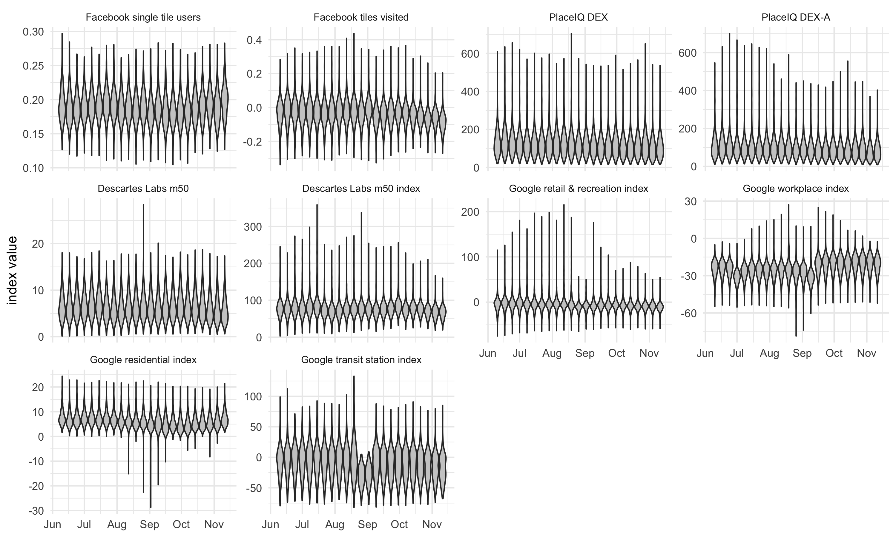
Figure 1: Violin plots of observed distributions of the ten mobility indices over time. Descriptions of the indices are provided in Appendix B.1.

To account for measured differences between counties on factors potentially influencing mobility and case rates (i.e., confounders), we collected a wide range of covariates from public sources. These spanned several domains: socioeconomic (ex: levels of poverty, unemployment, education, median household income, crowded housing, population density, urbanization); health-related (ex: rates of smoking and obesity, pollution, extreme temperatures); demographic (ex: distribution of age, race, sex); and political (ex: 2016 presidential election result, mask mandate level). Additionally, since the one-week-behind case rate could influence that week’s mobility (e.g., people may be less mobile if the perceived danger is higher) and subsequent transmission, previous week case rates were also included in the confounder set. The full list of variables collected and links to their sources are provided in Appendix B.3.

2.1 Data structure, causal model, & causal parameter

To assess impact over time while avoiding holiday- and weekday-level case reporting idiosyncrasies [36], mobility and case data were binned into weeks using a simple mean. We then repeated our analysis in cross-sectional snapshots over each week during the period beginning June 1, 2020 and ending November 14, 2020 separately for each mobility index. More formally, let $t=\{1,\ldots,24\}$ denote the week and $m=\{1,\dots,10\}$ denote the mobility index. Then for time $t$ and for mobility index $m$, let $W_{tm}$ denote the set of potential confounders, $A_{tm}$ the observed mobility level, and $Y_{tm}$ the new COVID-19 cases per 100,000 residents for a given county. We assumed that the following nonparametric structural equation model (NPSEM) characterized the county-level data generating process for week $t$ and mobility index $m$ [37]:

$$W_{tm} =f_{W_{tm}}(U_{W_{tm}})$$

$$A_{tm} =f_{A_{tm}}(W_{tm},U_{A_{tm}})$$

$$Y_{tm} =f_{Y_{tm}}(W_{tm},A_{tm},U_{Y_{tm}})$$ (1)

where $U_{W_{tm}}$, $U_{A_{tm}}$, and $U_{Y_{tm}}$ are unobserved random variables and $f_{W_{tm}}$, $f_{A_{tm}}$, and $f_{Y_{tm}}$ are unspecified (nonparametric) functions that may vary by mobility index and week. For each county $i=\{1,\dots,1182\}$, we assumed its observed data $O_{tmi}=(W_{tmi},A_{tmi},Y_{tmi})$ were generated by sampling from a distribution $\mathbb{P}_{0,tm}$ compatible with this causal model. With $T=24$ time points and $M=10$ mobility indices, we had $T\times M=240$ observed sets, each consisting of 1,182 observations (counties). As previously discussed, we conducted repeated cross-sectional analyses, taking each week and mobility index in turn. (Longitudinal approaches to examine the cumulative effects of mobility shifts over time were of great interest, but beyond the scope of this demonstration paper.) Importantly, we included the previous week’s new case levels in the confounder set for the effect of current mobility on cases two weeks later.

For ease of notation for the remainder of the paper, we will drop the subscripts denoting time $t$ and index $m$ when discussing the causal model $W=f_{W}(U_{W});A=f_{A}(W,U_{A});Y=f_{Y}(W,A,U_{Y})$, the observed data $O_{i}=(W_{i},A_{i},Y_{i})$ for county $i$, and the observed data distribution $\mathbb{P}_{0}$. We emphasize that this was to simplify notation; we are not introducing new assumptions that the data generating processes were common across time or exposure. Each causal and statistical analysis was specific to each week-mobility combination.

Following the MTP framework in [38], we generated counterfactual case rates $Y^{d}=f_{Y}(W,A^{d},U_{Y})$ by intervening on the causal model to shift the observed exposure by some user-specified function: $A^{d}=d(\cdot)$. While this shift function $d$ can depend on covariates, we focused on simpler interventions to shift the observed exposure $A$ by an additive constant $c$ or multiplicative constant $k$: $d(A,c)=c+A$ and $d(A,k)=k\times A$, respectively. By this definition, setting $c=0$ or $k=1$ recovers the observed exposure $A$ and the observed outcome $Y$.

For each index, we selected the scale and the shift amount to reduce mobility based on the index’s definition and range of observed values (Figure 1; Appendix B.1). For example, Facebook’s “single tile user” is a proportion of users who stayed in a single location (presumably, their residence) in a day and is thus bounded by 0 and 1. Based on its observed distribution (pooling over all follow-up weeks), we considered a relative increase of 5 percentage points in primary analyses and 7-8 percentage points in sensitivity analyses; all shifts were truncated at the upper bound of 1. For some indices, such as the DEX-A, which measures the density of mobile devices visiting commercial locations, larger shifts were reasonable; an example of a multiplicative shift of 0.75 to bring each county to 75% of its observed mobility is shown in the left panel of Figure 2. As a third example, consider Google’s “retail and recreation” index, defined as the percentage of visits to non-essential businesses relative to a pre-COVID baseline of 100%. Here, we examined additive shifts of -5 percentage points, bounded by the index limit of -100, shown in the right panel of Figure 2. A list of shifts examined for each variable is given in Appendix B.1.

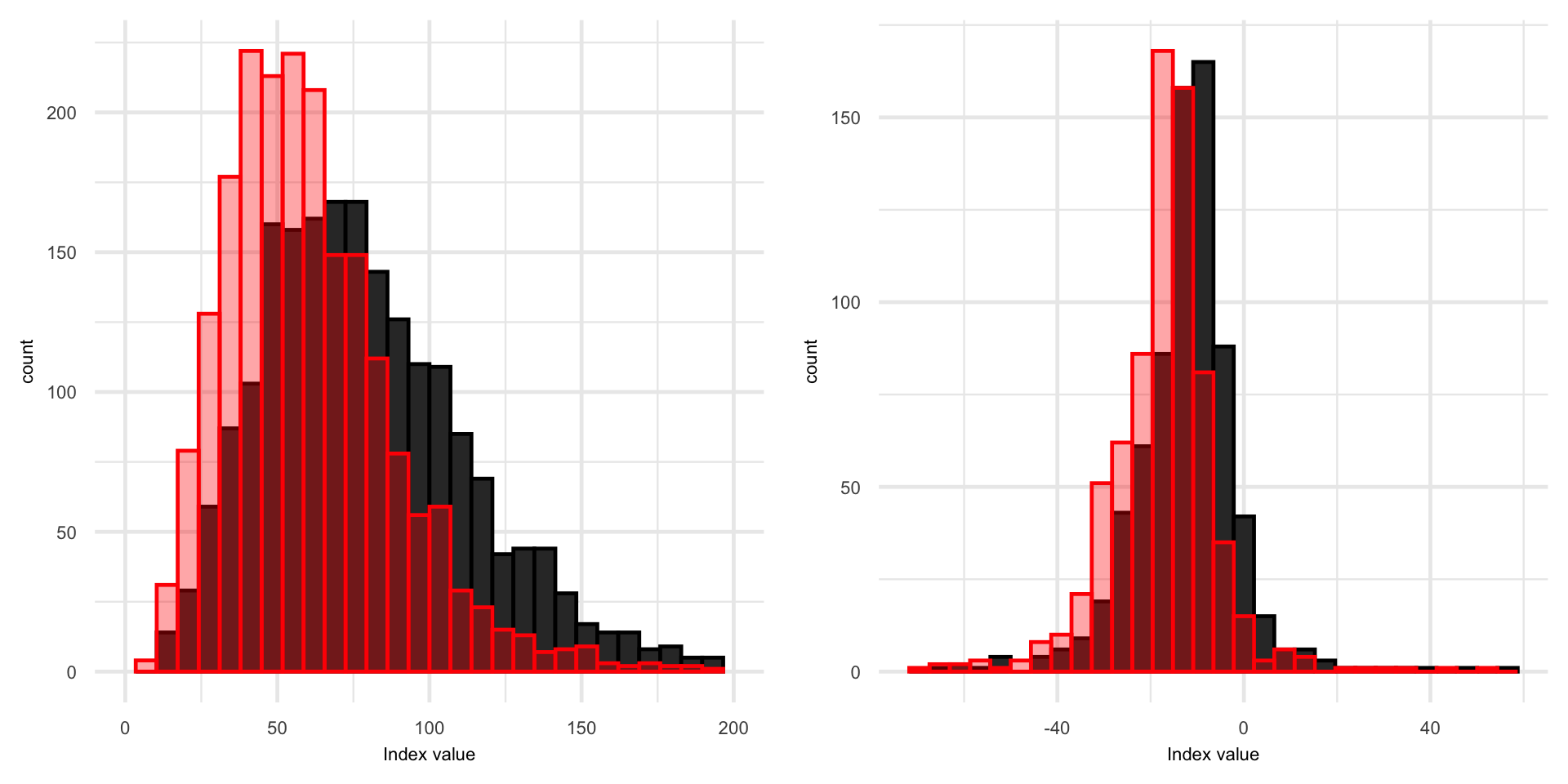
Figure 2: Examples of MTP interventions: a multiplicative shift of 0.75 in the distribution of DEX-A on August 26, 2020 (left) and an additive shift of -5 percentage points in the distribution of Google’s “retail and recreation” index on on August 26, 2020 (right). Observed values are shown in black, and shifted values in red overlay.

For each week and index, we specified our causal parameter $\phi$ as the difference in the expected counterfactual COVID-19 case rate under the shifted mobility and the expected COVID-19 case rate under the observed mobility:

$$\phi^{\Delta}=\mathbb{E}\left[Y^{d}\right]-\mathbb{E}\left[Y\right]$$ (2)

where the expectation is over the (most populous) U.S. counties of our target population.

2.2 Identification & the statistical estimand

For the causal parameter (Eq. 2, involving a summary measure of the distribution of counterfactuals) to be identified in terms of the observed data distribution, several assumptions would be required, discussed in more detail in Appendix C [22, 9, 38]:

• No unmeasured confounding: There are no unmeasured common causes of the mobility index and subsequent case rates, which we can formalize as $Y^{d}\perp\!\!\!\perp A|W$. In our context, this assumption would be violated if, for example, an unmeasured variable influenced both the county-level mobility and the case rate. One possible example could be issuing of and compliance with NPIs; an NPI might reduce mobility and also influence non-mobility-related behavior that is associated with future case rates. We attempted to improve the plausibility of this assumption by considering a very large confounder set including known correlates for our outcome and exposure. Nevertheless, we cannot guarantee that this assumption holds, and therefore limit our interpretations to statistical associations rather than causal effects.

• Positivity: If $(a,w)$ is within the support of $A,W$, then $(d(a,c),w)$ for additive shifts or $(d(a,k),w)$ for multiplicative shifts must also be within the support of $A,W$. In practice, this means that for any given time-slice and set of adjustment covariates, there is a positive probability of finding a county with the same covariate values and a mobility level matching the shifted value. We attempted to improve the plausibility of this assumption by first screening for instrumental variables (Appendix B.3) and then considering small shifts, which avoided extreme density ratios (described below and in Appendix B.1), while recognizing that this approach makes our causal effect data-adaptive.

The additional assumptions of independence between counties, consistency, and time-ordering were already made when specifying the causal model in Eq. 1 and discussed further in Appendix C.

If these identifiability assumptions held, we could specify and focus our estimation efforts on a statistical estimand that equals the wished-for causal effect. In the (likely) case that they are not satisfied, we could still specify and focus our estimation efforts on a statistical estimand that is as close as possible to the causal parameter. Factoring the joint distribution of the observed data $\mathbb{P}_{0}$ into $\mathbb{P}_{0}(O)=\mathbb{P}_{0}(Y|A,W)\mathbb{P}_{0}(A|W)\mathbb{P}_{0}(W)$, Haneuse and Rotnitzky showed [9] that the statistical estimand corresponding to expected counterfactual outcome under shift $d$, $\mathbb{E}[Y^{d}]$, is given by

$$\psi_{0}(A^{d})=\int\mathbb{E}(Y\mid A=a^{d},W=w)\text{d}F_{A,W}(a,w),$$ (3)

with $\text{d}F_{A,W}(a,w)$ as the joint density of received exposures $A$ and covariate levels $W$ being integrated over, equivalent to the extended g-computation formula of Robins et al. [39]. Here and throughout, the subscript $0$, indexing the statistical parameters, is used to emphasize these are functions of the observed data distribution $\mathbb{P}_{0}$. We refer to $\psi_{0}(A^{d})$ as the “shift parameter.” Under no shift, the expected outcome was trivially identified as $\psi_{0}(A)=\mathbb{E}(Y)$. Therefore, our statistical estimand of interest, corresponding to the expected difference in COVID-19 case rates under shifted and observed mobility ($\phi^{\Delta}=\mathbb{E}\left[Y^{d}\right]-\mathbb{E}\left[Y\right]$, given in Eq. 2), was

$$\psi^{\Delta}_{0}=\psi_{0}(A^{d})-\psi_{0}(A)=\int\mathbb{E}(Y\mid A=a^{d},W=w)\text{d}F_{A,W}(a,w)-\mathbb{E}(Y).$$ (4)

All shifts we examined were reductions in mobility; hence, under this definition, we expected $\psi_{0}^{\Delta}$ to be negative if mobility reductions were associated with lower case rates. We reiterate that each of the causal and statistical parameters were specific to the week $t$ and mobility index $m$, but additional subscripting is suppressed for notational convenience.

2.3 Estimation and inference

To estimate the expected outcome under the observed exposure $\psi_{0}(A)=\mathbb{E}(Y)$, we used the empirical mean outcome. For estimating the shift parameter $\psi_{0}(A^{d})$, given in Eq. 3, we used TMLE [10, 11]. TMLE is a general framework for constructing asymptotically linear estimators with an optimal bias-variance tradeoff for a target parameter. Typically, TMLE uses the factorization of the observed data distribution into an outcome regression $\bar{Q}(A,W)=\mathbb{E}(Y\mid A,W)$ and an intervention mechanism $g(A\mid W)=P(A\mid W)$. Then, an initial estimate of the outcome regression $\bar{Q}$ is updated by a fluctuation that is a function of the intervention mechanism. The update step tilts the preliminary estimates toward a solution of the efficient influence function estimating equation, endowing it with desirable asymptotic properties such as double-robustness, described in Appendix D. Further, it allows practitioners to utilize machine learning algorithms in the estimation of $\bar{Q}$ and $g$ while still maintaining valid statistical inference under regularity and convergence conditions [10].

TMLE is a general framework; the exact algorithm may vary depending on the data structure and question of interest. In this application, we used the implementation of Díaz [38] and refer the reader to their paper for the technical details. Here, we summarize briefly the algorithm for the shift parameter $\psi_{0}(A^{d})$, given in Eq. 3; we again emphasize that we repeated these analyses for each of the 240 week-mobility combinations.

First we defined the density ratio

$$r(a,w) =\frac{g^{d}(a|w)}{g(a|w)}$$ (5)

where $g^{d}(a|w)$ is the conditional density of $a$ under the shifted distribution and $g(a|w)$ the conditional density as observed. Unfortunately, estimating the conditional density $g$ directly can be difficult in high dimensions. Few data-adaptive algorithms exist [38], and for those that do [40], computation time can be demanding and data sparsity can make estimates unstable. Luckily, an equivalent estimate for $r$ can be found by recasting it as a classification problem [38]. In this formulation, a data set consisting of two copies of each observation is created, one assigned the observed exposure and one the shifted exposure. Further, each is given an indicator $\Lambda$ for whether it received the natural or shifted value of treatment. Using Bayes’ rule and the fact that $P(\Lambda=1)=P(\Lambda=0)=.5$,

$$r(a,w)=\frac{g^{d}(a|w)}{g(a|w)} =\frac{P(a,w\mid\Lambda=1)}{P(a,w\mid\Lambda=0)}=\frac{P(\Lambda=1\mid a,w)}{P(\Lambda=0\mid a,w)}$$ (6)

$$=\frac{P(\Lambda=1\mid a,w)}{1-P(\Lambda=1\mid a,w)}.$$

In this formulation, the density ratio estimate can be calculated as a function of $P(\Lambda=1\mid a,w)$, which can be estimated using any binary classification method and which we will write as $\tilde{\lambda}$. This innovation by Díaz [38] drastically improved computation time compared to estimating $g$ directly (as was done in several algorithms for stochastic interventions [41, 42]).

To implement estimation of $\tilde{\lambda}$ and the conditional outcome regression $\bar{Q}$ flexibly, we used the ensemble machine learning algorithm Super Learner[43], allowing us to avoid the parametric assumptions inherent in relying on a single regression model and, instead, to harness the strengths of multiple approaches, including nonparametric algorithms. Super Learner creates a convex combination of candidate algorithms chosen through cross-validation to minimize a user-specified loss function. In our case, the Super Learner ensemble included generalized linear models, generalized additive models, gradient boosted decision trees, random forest, and a simple mean.

Given estimates of the nuisance functions $\bar{Q}$ and $\tilde{\lambda}$, Appendix D outlines step-by-step estimation of the shift parameter $\psi_{0}(A^{d})$ and then the association of interest $\psi_{0}^{\Delta}$. The Appendix also discusses asymptotic properties of TMLE, under specific regularity and convergence conditions [10], and how those asymptotic properties can be used to generate Wald-style 95% confidence intervals from the estimated influence curve of $\hat{\psi}^{\Delta}$. All statistical analyses were performed in R version 4.0.3 [44], in particular the ltmp_tmle function in the lmtp package [45]. Code and data for reproduction are available at https://github.com/joshua-nugent/covid-mtp.

3 Results

Figure 3 shows estimates of $\hat{\psi}^{\Delta}$, the difference between the COVID-19 case rate that would be expected under the shifted distribution, after adjusting for measured confounders, and the observed average case rate, with associated 95% confidence intervals (CIs), for each of the mobility indices and weekly time slices from June 1, 2020 to November 14, 2020. For comparison, we also show unadjusted estimates, which is defined analogously to $\hat{\psi}^{\Delta}$, simply without any covariates $W$.

As an example, consider the first panel of Figure 3, showing $\hat{\psi}^{\Delta}$ for “Facebook single tile users,” which measures the proportion of mobile devices in a county that stayed in a single location (presumably, a home) each day, averaged over the week. In the first time-slice (June 1, 2020), the unadjusted results, in gray, showed a small association between reduced mobility (5% increase in the proportion of people staying at home) and new case rates: -3.2 (95%CI: -4.4, -1.9) cases per 100,000 residents two weeks later. After adjusting for confounders (in red), the association shrunk to -0.7 (-2.2, 0.7). In the week of September 28, the results were similar but more extreme: a 5% increase in the proportion of people staying at home in the unadjusted analysis suggested a change of -16.0 (-18.6, -13.3) in new cases per 100,000 residents two weeks later, while that association was attenuated to -4.5 (-7.0, -2.0) after confounder adjustment. Across all of the time slices for that mobility index, we saw the same pattern. Unadjusted estimates of $\hat{\psi}^{\Delta}$ varied, but were negative, as we would expect; lower mobility appeared to be associated with lower new case rates. After adjustment, however, the estimates shrunk towards zero and many of the CIs overlapped with zero.

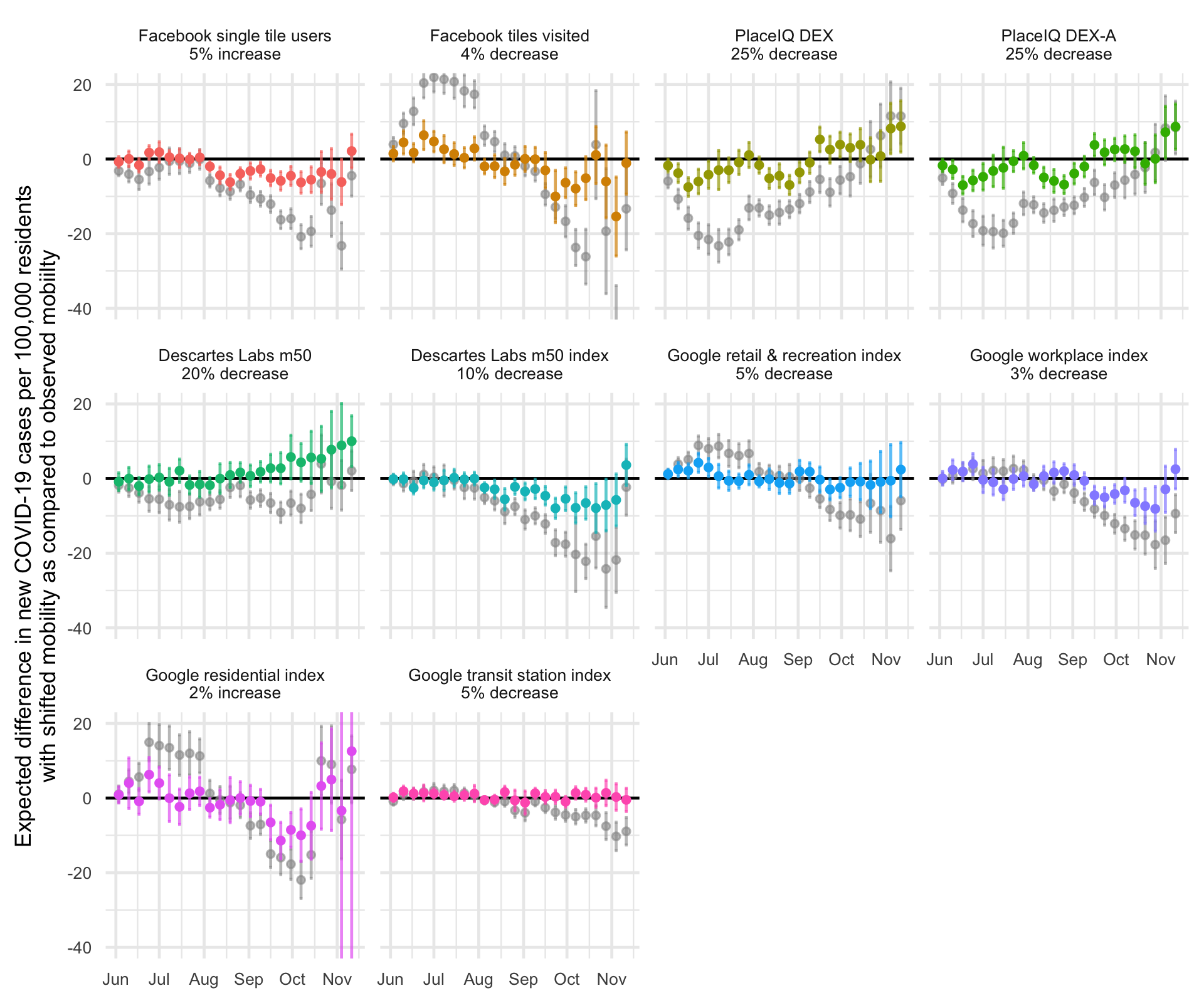
Figure 3: Difference in mean predicted case rates two weeks ahead with shifted distribution vs. observed case rates for weekly time slices from June 1 - November 14, 2020. Unadjusted analyses show some correlation between mobility and case rates (gray values with 95% CIs below the null line of 0), but after adjustment (colored values), no indices show consistent associations across the weeks examined. For most indices, the majority of confidence intervals include 0 after adjustment. Recall that the two stay-at-home measures, Facebook’s ‘single tile users’ and Google’s ‘residential’, were assigned positive shifts, which corresponded to a reduction in mobility.

Broadening the scope to all indices in Figure 3, some patterns emerged. First, almost all unadjusted associations were larger than the adjusted ones, although point estimates were usually in the same direction after adjustment. Second, CIs increased in October and November, suggesting higher outcome variance, more treatment effect variability, or higher density ratios (perhaps from near practical positivity violations). Third and most notable, after adjustment for our confounder set, associations were generally small; CIs overlapped with zero, and point estimates showed almost no consistent trends of positive or negative association.

For example, only six of the indices showed even short-term consistent associations with the outcome after adjustment, perhaps due to seasonal effects: Facebook’s ‘single tile users’ metric (Aug, Sept, Oct), PlaceIQ’s ‘DEX’ and ‘DEX-A’ measures of device density (Jun, Aug), Decartes Labs ‘m50 index’ of distance traveled from the home (Aug, Sept, Oct), Google’s workplace index (Sept, Oct), and Google’s stay-at-home residential index (Sept, Oct). However, these same indices had uncertain associations in other time periods, with CIs overlapping zero, and in several instances had point estimates (and sometimes and CIs) unexpectedly above zero.

Surprisingly, three indices showed positive unadjusted point estimates in June and July (Facebook ‘tiles visited’ and Google’s ‘retail & recreation’ and ‘residential’ indices), with Facebook’s ‘tiles visited’ index showing an unusually large swing between summer and fall. After adjustment, the estimates were strongly attenuated. We performed several sensitivity analyses that did not meaningfully change our results (Appendix E).

4 Discussion

To the best of our knowledge, we are the first to apply MTPs to study the effects of shifting the distribution of a continuous exposure in an infectious disease setting; specifically, we aimed to answer the question of whether reductions in mobility, as captured by mobile phone data, led to reductions in subsequent COVID-19 case rates across U.S. counties in the summer and fall of 2020. We also hope this paper will serve as a demonstration of how the MTP approach can be used by other researchers to nonparametrically define causal effects with continuous exposures; in our case, we examined the impact of additive and multiplicative shifts of the observed exposure distribution. More commonly, continuous exposures are handled by discretizing into binary ‘high’ / ‘low’ categories (which may be defined arbitrarily, or violate positivity assumptions), or, alternatively, the causal “dose-response” curve is summarized with an MSM, relying on strong parametric assumptions (i.e., a generalized linear model to relate the expected counterfactual outcome to the continuous exposure). Additionally, by defining the intervention as a function of the observed exposure value, MTPs can help us to define causal effects that are better supported by the data.

The MTP approach is also simple to implement in software. The recent innovation by [38] to recast estimation of density ratios into a binary classification problem overcomes many of the prior computational challenges for estimation of statistical parameters corresponding to MTPs and stochastic interventions. This innovation is integrated into ltmp R package, which also provides doubly-robust and flexible estimation through TMLE with Super Learner, making it a powerful off-the-shelf option for researchers seeking to implement MTP. Altogether, we believe the MTP framework is an attractive and under-utilized approach to studying the effects for continuous exposures.

Our application of MTP to investigate the relationships between mobility and new COVID-19 case rates suggested that associations varied over time. Although our unadjusted analyses seem to suggest that decreased mobility was associated with reductions in COVID-19 case rates for the majority of timepoints examined, adjusted analyses were strongly attenuated with most 95% confidence intervals crossing the null value. This provides evidence that unadjusted associations may be highly confounded by county characteristics and current case rates. For example, our adjustment set included variables for county-level political lean, which may be a proxy for adherence to NPIs like mask-wearing mandates. It could appear that counties with lower mobility have fewer new cases, but if low-mobility counties are also more consistently adhering to mask-wearing due to underlying political dynamics, the association with mobility would be attenuated after adjustment. Including one-week lagged case rates in the adjustment set could also help control for confounding by epidemic arrival time and intensity. Our results contextualize and help explain findings in the earlier research, outlined in Appendix A, which showed mixed associations depending on the timeframe, mobility index, geographic area, and potential confounder set considered.

There are several limitations to our application, some of which may explain the inconsistent patterns of association seen over time and suggest avenues for future investigation. First, while we chose a timeframe when COVID testing was widely available, differential ascertainment of case rates across counties could bias our estimates. Similarly, while we examined ten distinct mobility indices, we recognize that each is a proxy for underlying mobility patterns in a given county. While we controlled for factors potentially related to use of mobile phones and certain apps (e.g. Facebook), such as age, we cannot rule out the potential for measurement error in the exposure and therefore the potential for bias in our results. Second, while county-level mobility and covariate data were easily accessible, there might be important sub-county level effects that were masked when aggregating to the county-level. Performing this analysis at the zip code or census tract level might reveal stronger or more consistent associations. Indeed, a minimally adjusted analysis of zip-code level mobility data and case rates in five cities [46], while finding a strong association, also reported substantial heterogeneity across space and time. On the other hand, the policy relevance of such results is complicated considering that most public heath measures aiming to limit close contacts (and, indirectly, mobility) are implemented at the county and state level. Third, our assumption of independence between counties is unlikely to hold, given state-level policy enactment and spillover effects between counties. Indeed, the results of spatial and network dependence can be unpredictable [47]; so we hesitate to speculate about the directions in which they might have biased our point estimates or standard errors, but they are likely in play. Fourth, despite our large adjustment set, it is possible that we excluded important confounders, or that we have unmeasured confounding, as is common with observational data. For example, we had no data on the strength of a county’s public health infrastructure or compliance with NPIs, which could presumably impact both the mobility and case rates.

Fifth, while MTPs relax the positivity assumptions of binary, static interventions (requiring all levels of the exposure to be supported within all possible values of adjustment variables [12]), MTPs do require support within the shift value. While reasonable in theory, this is only practically supported when the specified shifts $A^{d}$ are not “too” drastic and the adjustment set $W$ not “too” large. Here, we examined the largest shifts possible where the mobility-specific density ratio $r(a,w)$ was consistently less than 10, which we took as a reasonable cutoff for practical positivity violations. This meant that examining extreme shifts was not possible, because during the study period many counties already had significantly reduced their mobility compared to pre-pandemic baselines. However, sensitivity analyses examining slightly larger shifts, still somewhat supported by the data, yielded similar results (Appendix E.4). If mobility index data were available for the sparsely populated counties that we excluded, it might be possible to expand our target population and investigate a wider range of shifts that might detect stronger or more consistent associations. Indeed, the MTP approach will generally be more informative when a large range of shifts are supported by the data.

Sixth, there are still many unknowns about the dynamics of COVID transmission over space and time as well as their interplay with human behavior. Including one week lagged case rates in our adjustment set may have helped address some of those unknowns, but is likely not able to account for all of the complex dynamics of COVID transmission. For example, the return to schools in Fall 2020 may partially explain how several indices show different behavior in the summer and fall: the adjusted DEX and DEX-A point estimates change sign and the adjusted m50 estimates shift from minimal associations to stronger ones. Additionally, while MTPs facilitated our examination of shifting the mobility distribution, we did not explicitly discuss the policies, such as non-essential business closures, that could generate such shifts. Instead in this demonstration paper, we sought to understand if these mobility indices were consistently associated with subsequent COVID-19 case rates; they were not. Finally, our choice of a cross-sectional time-series analysis in weekly slices may have hidden complex patterns over time. A longitudinal analysis that examines the full scope of mobility over time and its impact on cumulative cases per capita could provide a more complete view of the full impact (or lack thereof) of these mobility indices on case transmission.

5 Conclusion

Altogether, our applied analysis suggested that county-level mobility indices are not generally associated with reductions in subsequent COVID-19 case rates, after adjusting for a wide range of measured confounders. Our analysis, founded in a causal inference framework [48, 49, 50], also highlighted some of the limitations of prior research in this area, including measurement error, dependence between observational units, unmeasured confounding, limited data support, and the many unknowns about COVID-19.

Nonetheless, using MTP allowed us to consider shifts in mobility supported by our observed data, and TMLE allowed for the leveraging of machine learning to minimize parametric assumptions while still providing the basis for valid statistical inference. MTPs can be useful tool for studying the impacts of continuous exposures in epidemiology and beyond.

Appendix A Brief review of the literature on mobility & COVID-19 transmission

Recent papers investigating the associations between mobility, COVID-19 spread, and NPIs can be roughly categorized into one of three bins: work that uses mobility as an input into a more complex model to forecast COVID-19 cases and deaths (see, e.g., [51, 52, 53]); work that assesses the effectiveness of, or compliance with, NPIs, using mobility as an outcome variable (see, e.g., [54, 55, 56, 57, 58, 59]); and finally work that treats mobility as an exposure variable and new COVID-19 case rates or deaths as the outcome. This work falls in the last category.

Most papers focusing on the early-pandemic (Spring 2020) timeframe found strong correlations between mobility and COVID-19 spread [31, 30, 60, 61, 59]. However, these early studies are potentially confounded by the spatial dynamics of where the pandemic arrived first and unmeasured variables such as underlying changes in behavior including mask-wearing or the propensity to socialize outdoors rather than in closed indoor environments (see, e.g., the heterogeneity identified by [58]). In addition, they may be subject to bias from undercounted cases due to lack of testing capacity in many parts of the U.S. [62]. Given these challenges, it is perhaps unsurprising that the associations between mobility and COVID-19 cases were strongly attenuated in studies extended through mid-Summer of 2020 [63, 64].

Our findings on how the associations between mobility and COVID spread vary over time and with confounder adjustment are in line with other results. In an analysis using data from the 25 hardest-hit U.S. counties through mid-April 2020, Badr et al. [30] fit an unadjusted statistical model for future case growth rates based on a mobility measure using number of trips made per day compared to a pre-pandemic baseline. While strong associations were found between changes in their mobility index and county-level case growth 9-12 days later, a later updated analysis [63], using data through September 16 and expanding the dataset to all U.S. counties, showed that the association disappeared after April. Similarly, Gatalo et al. [64], using a slightly different methodology, found strong correlations between mobility and case growth from March 27 to April 20, but only a weak correlation from then until July 22. Another analysis [60], using data through June 9, 2020, treated the inflow of traffic into a county as the exposure, adjusted for a small number of socio-demographic covariates, and found a strong relationship between inflow and new cases 7 days later. Finally, an examination [31] of the correlations between Google’s six mobility indices (retail & recreation, transit stations, workplaces, residential, parks, grocery & pharmacy) and 11-day ahead case growth rates at the county level, stratifying by urban-rural classification, suggested strong associations in the February to April timeframe, especially in more dense counties, but those correlations were weaker when the timeframe was extended to June.

Our work adds to other evidence of confounding in COVID-19 research; for example, McLaren [65] found that some correlations between racial/ethnic groups and COVID-19 mortality disappeared once confounding factors were taken into account, and Wong and Balzer [50] found that associations between mask mandates and future case rates were attenuated after confounder adjustment. We suspect this confounding may explain why our results contradict those of Wellenius et al. [59], who found that mobility levels (using many of the same county-level metrics) in Spring 2020 were strongly associated with COVID case growth rates two weeks later. Their work differed from this analysis in that the researchers did not include any socioeconomic covariates in their parametric model (suggesting a different causal parameter and estimation approach) nor extend their analysis beyond March and early April.

Appendix B Data details

B.1 Mobility index sources, definitions, and shifts considered

Below are the source and the description of each of the ten mobility indices examined. For each, we chose the reported intervention shift value by: (i) examining the observed exposure distribution, given in Figure 1 of the main text; (ii) selecting a set of shifts that seemed to have reasonable support; and (iii) of those, selecting the largest shift that yielded an estimated density ratio $\hat{r}(a,w)=\frac{\hat{g}^{d}(a|w)}{\hat{g}(a|w)}<10$. Recall $g^{d}(a|w)$ is the conditional density of $a$ under the shifted distribution and $g(a|w)$ the conditional density as observed.

Facebook Movement Range

• Single tile users: Percentage of people who stay in a single ‘Bing tile’ (roughly 600 m by 600 m) over an entire day. We examined multiplicative shifts of 1.05, 1.07, and 1.08, and used 1.05 in the primary analysis.

• Tiles visited: Percentage change in the number of Bing tiles a device pinged in a given day, compared to the baseline average for that weekday in February 2020, excluding Presidents’ Day, aggregated at the county level. We examined additive shifts of -3 and -4, and used -4 in the primary analysis.

PlaceIQ

• Device exposure index (DEX): Counts the number of distinct devices that entered the same commercial spaces that day as the target device, then averages that number across all devices in the county. We examined multiplicative shifts of 0.75, 0.7, and 0.65, and used 0.75 in the primary analysis.

• Adjusted DEX (DEX-A): Scaled version of the DEX that adjusts for the possibility of devices sheltering in place, generating no pings, and hence not having their zero-DEX values be counted in the overall average. We examined multiplicative shifts of 0.75, 0.7, and 0.65, and used 0.75 in the primary analysis.

Descartes Labs

• m50: Median maximum distance traveled from starting location by all tracked devices in a county. We examined multiplicative shifts of 0.6, 0.7, and 0.8, and used 0.8 in the primary analysis.

• m50 index: Relative value of m50 relative to median baseline value for that day of the week between February 2, 2020, and March 7, 2020. We examined multiplicative shifts of 0.9 and 0.85, and used 0.9 in the primary analysis.

Google COVID-19 Community Mobility Reports

For Google indices, all of the baseline values are defined as the median value for that day of the week from January 3, 2020 to February 6, 2020.

• Retail & recreation: Percentage point change in number of visits and length of stay from baseline for restaurants, malls, movie theaters, and retail stores (excluding grocery stores and pharmacies). We examined additive shifts of -4, -5, and -6, and used -5 in the primary analysis.

• Workplace: Percentage point change in number of visits and length of stay from baseline for an individual’s place of work. We examined additive shifts of -2, -3, and -4, and used -3 in the primary analysis.

• Residential: Percentage point change from baseline of duration time spent at one’s residence each day. Since the baseline values are high, the variation in this index was smaller than the others. We examined additive shifts of +1, +2, and +3, and used +2 in the primary analysis.

• Transit station: Percentage point change in number of visits and length of stay from baseline for mass transit stations (buses, subways, etc). We examined additive shifts of -5, -10, and -15, and used -5 in the primary analysis.

B.2 Comparison of counties included/excluded

All mobility indices require sufficient sample size within a county to report reliable data on a given day. In low-population counties, this can make the mobility data sparse or nonexistent over the timeframe in question. Hence, to improve comparability across different indices and address positivity violations, we restricted our analysis to counties with 40,000 or more residents. The table below compares the covariate distribution across the included/excluded counties. While a vast number of counties were excluded, they represent only 10% of the U.S. population, and, with the exception of measures of population and 2016 presidential election results, their covariate means were similar to the counties included.

	All counties	Included	Excluded
N	3,158	1,182	1,926
Mean population	105,362	250,886	16,053
Mean population density (/sq. mi)	27,167	62,366	5,608
% Adults without health insurance	14.3%	13%	15%
% Under 18	22.3%	22.6%	22.2%
% Households below poverty line	15.2%	13.8%	16.1%
% Hispanic	9.3%	10.8%	8.4%
% Women	49.9%	50.6%	49.5%
% Black	8.9%	9.9%	8.5%
% Clinton vote in 2016 election	31.7%	38.6%	27.8%
% Drive alone to work	79.2%	80.5%	78.9%

B.3 Adjustment variables and their sources

We gathered a rich set of social, economic, physical, and demographic variables $W$ from the U.S. Census American Community Survey, U.S. Bureau of Labor Statistics, U.S. Centers for Disease Control, U.S. Department of Agriculture, University of Washington Population Health Institute and Department of Political Science, National Oceanic and Atmospheric Administration, and MIT Election Data and Science Lab.

Given plausible concerns about data support and desire to avoid controlling for instrumental variables, we reduced the adjustment set $W$ to eight variables for each index, based on which had the strongest univariate associations with the exposure (mobility index) and outcome (leading new cases per 100,000 people), pooled over all weeks. In sensitivity analyses (Appendix E), we also tested strategies where (i) covariates were chosen week-by-week instead of being held constant across all time slices and (ii) a smaller covariate set was chosen to make possible examinations of larger shift values without practical positivity violations. These sensitivity analyses produced similar results to our main analysis.

The primary analyses included the following covariates in the adjustment set:

• U.S. Census American Community Survey

  • Percentage of households below the poverty line

• University of Washington Population Health Institute, via Robert Wood Johnson Foundation County Health Rankings

  • Percentage of people that identify as Black

  • Percentage of people that identify as Hispanic

  • Percentage of people that drive alone to work

  • Percentage of people that are women (note: values under 49% are often an indicator of a large prison being in the county)

  • Percentage of people that are under 18 years of age

  • Percentage of adults without health insurance

• MIT Election Data and Science Lab

  • Percentage of vote for Hillary Clinton in the 2016 Presidential election

The following covariates were also examined, but not included in the primary analysis.

• U.S. Census American Community Survey

  • Population density

  • Natural logarithm of population density

  • Average household size

  • Percentage of people living below the poverty line

  • Percentage of households with income below the poverty line

  • Percentage of people in the county who live outside of a metropolitan area

• University of Washington Population Health Institute, via Robert Wood Johnson Foundation County Health Rankings

  • Percentage of adults who smoke

  • Percentage of people that identify as Asian

  • Percentage of people that are 65 years of age or older

  • Percentage of people with more than a high school education

  • Index of income inequality

  • Natural logarithm of median household income

  • Level of air particulate matter (pollution)

• State-level social distancing policies in response to the 2019 novel coronavirus in the U.S., University of Washington Department of Political Science

  • Mask mandate level (statewide data only)

• Centers for Disease Control and Prevention

  • Percentage of people who live in crowded housing

  • Percentage of people categorized as obese

  • Percentage of people living with diabetes

• National Oceanic and Atmospheric Administration

  • Absolute daily high temperature deviation from 70 degrees Fahrenheit

• U.S. Bureau of Labor Statistics

  • Unemployment rate

• U.S. Department of Agriculture

  • Presence of a level 5 meatpacking plant (largest plants)

  • Presence of a level 4 meatpacking plant (second largest plants)

  • Presence of a level 4 or level 5 meatpacking plant

Appendix C Details of identification assumptions

Beyond no unmeasured confounding and positivity, there are three additional assumptions that are implied by our adoption of the NPSEM. (1) Independence of counties. This independence assumption is likely violated since there were state-level policies (e.g., stay-at-home orders) that plausibly created dependence between counties in a state. The independence assumption also implies no interfence: The exposure level $a$ for a given county does not affect the outcomes of the other counties. Given that infectious disease spread does not respect town, county, state, or country boundaries, this assumption may be unrealistic. (2) Consistency: If $A=a$ for any county, then $Y(a)=Y$, and hence the full observed set of outcomes when $A^{d}=A$ is simply $Y(A^{d})=Y$. This means that the counterfactual outcome for a county with its observed mobility level is the observed outcome. This assumption is implied by our definition of counterfactuals as derived quantities through interventions on the NPSEM. (3) Time-ordering: The confounders $W$ precede the mobility exposure $A$, which also precedes the case rate outcome $Y$.

Appendix D Estimation and inference

Recall from section 2.3 that we used Super Learner to obtain nuisance function estimates for the conditional mean outcome $\bar{Q}$ and the density ratio $\tilde{\lambda}$. Given these estimates, we first describe how to estimate the shift parameter $\psi_{0}(A^{d})$ and then the associational parameter $\psi_{0}^{\Delta}$. The following steps have been modified for a cross-sectional analysis (i.e., a single week $t$ and a single index $m$) from the longitudinal version of [38]. In practice, we note that our bounded continuous outcome will be scaled to $[0,1]$ (see [66]) before estimation of the conditional mean outcome $\bar{Q}$ and before the steps below.

• Define and calculate the density ratio under the specified shift $\hat{r}(a_{i},w_{i})$ for each county $i=1,...,n$ from $\tilde{\lambda}$ estimated via Super Learner.

• Generate initial conditional expectations for each county, denoted $\bar{Q}(A,W)$.

• Fit the following logistic regression on the observed (scaled) $Y$ values, using the logit of the initial estimates as an offset

  $$\text{logit}(\bar{Q}^{*}(A,W))=\text{logit}(\bar{Q}(A,W))+\epsilon$$

  with weights $\hat{r}(a_{i},w_{i})$, calculating the estimated intercept $\hat{\epsilon}$, where $\bar{Q}^{*}(A,W)$ is now a targeted estimate of the conditional mean outcome.

• Use the resulting $\hat{\epsilon}$ value to generate targeted predictions under a shift, $\bar{Q}^{*}(A^{d},W)$:

  $$\bar{Q}^{*}(A^{d},W) =\text{logit}^{-1}\left[\text{logit}(\bar{Q}(A^{d},W))+\hat{\epsilon}\right].$$

With the updated estimates $\bar{Q}^{*}(A^{d},W)$ in hand (after unscaling), define $\hat{\psi}_{tmle}$ as:

$$\hat{\psi}_{tmle}=\frac{1}{n}\sum_{i=1}^{n}\bar{Q}^{*}(A^{d},W).$$

This TMLE estimator is “doubly-robust” in that it is a consistent estimator of $\psi_{0}(A^{d})$ if estimation of either $\bar{Q}$ or $\tilde{\lambda}$ is consistent. Further, if both are consistent, along with certain regularity conditions and multiplicative $\sqrt{n}$ convergence rates [10], the TMLE converges to a normal distribution with mean 0 and variance equal to the nonparametric efficiency bound, as shown in Theorem 3 of [38]. The efficiency bound for this TMLE depends on the variance of the outcome conditional on $A$ and $W$, the amount of treatment effect variability, and the intensity of shift applied, as measured by the density ratio $r(a,w)$ [38].

The inclusion of a wide variety of algorithms in our Super Learner ensemble improves our chances of meeting the required regularity conditions and, thus, obtaining an asymptotically linear estimator, which is normally distributed in the large data limit. Additionally, since recent work [67] has highlighted the danger that tree-based algorithms may not meet required convergence rates or the Donsker condition, we reran the analyses excluding random forest and gradient boosting from our Super Learner. The exclusion of these algorithms did not notably change our results. Future work using cross-validation (a.k.a. cross-fitting) as part of the estimation process would obviate the Donsker condition and allow for more aggressive machine learning algorithms to be included.

Using the empirical mean $\bar{Y}=\frac{1}{n}\sum_{i=1}^{n}Y_{i}$ to estimate $\psi_{0}(A)=\mathbb{E}(Y)$, we obtain an estimate of the statistical association parameter $\psi_{0}^{\Delta}=\psi_{0}(A^{d})-\psi_{0}(A)$ with

$$\hat{\psi}^{\Delta}=\hat{\psi}_{tmle}-\bar{Y}.$$

Under the above conditions, TMLE is an asymptotically linear estimator of the shift parameter $\psi_{0}(A^{d})$ with influence curve $IC^{d}(O)=r(A,W)[Y-\mathbb{E}\left[Y\mid A,W\right]]+\mathbb{E}\left[Y\mid A^{d},W\right]-\mathbb{E}\left[Y(A^{d})\right]$[38]. Furthermore, the empirical mean $\bar{Y}$ is a linear estimator of the population mean $\psi_{0}(A)$ with influence curve $IC(O)=(Y-\bar{Y})$. By applying the Delta Method, we obtain the influence curve for the TMLE of the associational parameter $\psi_{0}^{\Delta}$:

$$IC^{\Delta}(O) =IC^{d}(O)-IC(O)$$

$$=r(A,W)[Y-\mathbb{E}\left[Y\mid A,W\right]]+\mathbb{E}\left[Y\mid A^{d},W\right]-\mathbb{E}\left[Y(A^{d})\right]-(Y-\bar{Y}).$$

Replacing all of the terms above with the observed data $Y_{i}$ and the estimates from $\bar{Q}$ and $\tilde{\lambda}$ to calculate $\hat{IC}^{\Delta}(O_{i})$, the variance of $\hat{\psi}^{\Delta}$ is well-approximated by the sample variance of the influence curve:

$$Var(\hat{\psi}^{\Delta})=\frac{1}{n}\sum_{i=1}^{n}\hat{IC}^{\Delta}(O_{i})^{2},$$

allowing for the calculation of the 95% Wald-style confidence interval $\hat{\psi}^{\Delta}\pm 1.96\sqrt{Var(\hat{\psi}^{\Delta})}$.

Appendix E Sensitivity analyses

E.1 Using one-week leading case rates as outcome

E.2 Using current-week cases in the adjustment set instead of one-week lagged cases

E.3 Using a time-varying confounder set

We tested three of the indices allowing for a different confounder set $W$, screened in each week time-slice by univariate correlations with the exposure and outcome. As with the main analysis, the adjusted results (shown below for several shift value possibilities) show inconsistent patterns over time and CIs frequently overlap with zero.

E.4 Using a smaller confounder set with larger shifts

We tested three of the indices with a smaller, time-varying confounder set $W$ (four rather than eight), screened in each week time-slice by univariate correlations with the exposure and outcome, with larger shift values. As with the main analysis, the adjusted results (shown below for several shift value possibilities) show inconsistent patterns over time and CIs frequently overlap with zero.

References

- [1] Xiao Huang et al. “Twitter reveals human mobility dynamics during the COVID-19 pandemic” Publisher: Public Library of Science In PLOS ONE 15.11, 2020, pp. e0241957 DOI: 10.1371/journal.pone.0241957
- [2] Emanuele Pepe et al. “COVID-19 outbreak response, a dataset to assess mobility changes in Italy following national lockdown” Number: 1 Publisher: Nature Publishing Group In Scientific Data 7.1, 2020, pp. 230 DOI: 10.1038/s41597-020-00575-2
- [3] Victor Couture et al. “Measuring Movement and Social Contact with Smartphone Data: A Real-Time Application to COVID-19”, 2020 DOI: 10.3386/w27560
- [4] Song Gao et al. “Mapping County-Level Mobility Pattern Changes in the United States in Response to COVID-19”, 2020 DOI: 10.2139/ssrn.3570145
- [5] Google “COVID19 Community Mobility Reports” URL: https://www.google.com/covid19/mobility/
- [6] Facebook “Movement Range Maps - Humanitarian Data Exchange” URL: https://data.humdata.org/dataset/movement-range-maps
- [7] Caroline O. Buckee et al. “Aggregated mobility data could help fight COVID-19” In Science 368.6487, 2020, pp. 145–146 DOI: 10.1126/science.abb8021
- [8] Kyra H. Grantz et al. “The use of mobile phone data to inform analysis of COVID-19 pandemic epidemiology” Number: 1 Publisher: Nature Publishing Group In Nature Communications 11.1, 2020, pp. 4961 DOI: 10.1038/s41467-020-18190-5
- [9] S. Haneuse and A. Rotnitzky “Estimation of the effect of interventions that modify the received treatment” In Statistics in Medicine 32.30, 2013, pp. 5260–5277 DOI: 10.1002/sim.5907
- [10] Mark J. der Laan and Sherri Rose “Targeted Learning: Causal Inference for Observational and Experimental Data”, Springer Series in Statistics New York: Springer-Verlag, 2011 DOI: 10.1007/978-1-4419-9782-1
- [11] Mark J. der Laan and Sherri Rose “Targeted Learning in Data Science: Causal Inference for Complex Longitudinal Studies”, Springer Series in Statistics Springer International Publishing, 2018 DOI: 10.1007/978-3-319-65304-4
- [12] Maya L Petersen et al. “Diagnosing and responding to violations in the positivity assumption” Publisher: SAGE Publications Ltd STM In Stat Methods Med Res 21.1, 2012, pp. 31–54 DOI: 10.1177/0962280210386207
- [13] Oliver Bembom and Mark J. der Laan “A practical illustration of the importance of realistic individualized treatment rules in causal inference” In Electronic Journal of Statistics 1.none, 2007, pp. 574–596 DOI: 10.1214/07-EJS105
- [14] J.M. Robins “Marginal structural models” In 1997 Proceedings of the American Statistical Association, 1998, pp. 1–10
- [15] James M. Robins, Miguel Ángel Hernán and Babette Brumback “Marginal Structural Models and Causal Inference in Epidemiology” In Epidemiology 11.5, 2000 URL: https://journals.lww.com/epidem/Fulltext/2000/09000/Marginal_Structural_Models_and_Causal_Inference_in.11.aspx
- [16] Romain Neugebauer and Mark Laan “Nonparametric causal effects based on marginal structural models” In Journal of Statistical Planning and Inference 137.2, 2007, pp. 419–434 DOI: 10.1016/j.jspi.2005.12.008
- [17] Ted Westling, Peter Gilbert and Marco Carone “Causal isotonic regression” arXiv: 1810.03269 In arXiv:1810.03269 [stat], 2019 URL: http://arxiv.org/abs/1810.03269
- [18] Edward H. Kennedy “Nonparametric Causal Effects Based on Incremental Propensity Score Interventions” In Journal of the American Statistical Association 114.526, 2019, pp. 645–656 DOI: 10.1080/01621459.2017.1422737
- [19] Dominik Rothenhäusler and Bin Yu “Incremental causal effects” arXiv: 1907.13258 In arXiv:1907.13258 [stat], 2020 URL: http://arxiv.org/abs/1907.13258
- [20] Edward H. Kennedy, Zongming Ma, Matthew D. McHugh and Dylan S. Small “Non-parametric methods for doubly robust estimation of continuous treatment effects” In Journal of the Royal Statistical Society: Series B (Statistical Methodology) 79.4, 2017, pp. 1229–1245 DOI: https://doi.org/10.1111/rssb.12212
- [21] Vanessa Didelez, Philip Dawid and Sara Geneletti “Direct and Indirect Effects of Sequential Treatments” In arXiv:1206.6840 [stat], 2012 URL: http://arxiv.org/abs/1206.6840
- [22] Iván Díaz Muñoz and Mark van der Laan “Population Intervention Causal Effects Based on Stochastic Interventions” In Biometrics 68.2, 2012, pp. 541–549 DOI: 10.1111/j.1541-0420.2011.01685.x
- [23] James H. Stock “Nonparametric Policy Analysis” Publisher: [American Statistical Association, Taylor & Francis, Ltd.] In Journal of the American Statistical Association 84.406, 1989, pp. 567–575 DOI: 10.2307/2289944
- [24] Iván Díaz and Nima S. Hejazi “Causal mediation analysis for stochastic interventions” In Journal of the Royal Statistical Society: Series B (Statistical Methodology) 82.3, 2020, pp. 661–683 DOI: 10.1111/rssb.12362
- [25] Hooman Kamel et al. “Relationship between left atrial volume and ischemic stroke subtype” In Annals of Clinical and Translational Neurology 6.8, 2019, pp. 1480–1486 DOI: 10.1002/acn3.50841
- [26] Alan Hubbard et al. “Time-dependent prediction and evaluation of variable importance using superlearning in high-dimensional clinical data” Publisher: Lippincott Williams and Wilkins In The journal of trauma and acute care surgery 75.1 SUPPL1, 2013, pp. S53–S60 DOI: 10.1097/TA.0b013e3182914553
- [27] Kara E. Rudolph et al. “When effects cannot be estimated: redefining estimands to understand the effects of naloxone access laws” arXiv: 2105.02757 In arXiv:2105.02757 [stat], 2021 URL: http://arxiv.org/abs/2105.02757
- [28] The New York Times “Coronavirus (Covid-19) Data in the United States” original-date: 2020-03-24T23:41:39Z, 2020 URL: https://github.com/nytimes/covid-19-data
- [29] “Coronavirus Outbreak Stats & Data” In USAFacts URL: https://usafacts.org/issues/coronavirus/
- [30] Hamada S. Badr et al. “Association between mobility patterns and COVID-19 transmission in the USA: a mathematical modelling study” Publisher: Elsevier In The Lancet Infectious Diseases 0.0, 2020 DOI: 10.1016/S1473-3099(20)30553-3
- [31] Xiaojiang Li “Association Between Population Mobility Reductions and New COVID-19 Diagnoses in the United States Along the Urban–Rural Gradient, February–April, 2020” In Prev. Chronic Dis. 17, 2020 DOI: 10.5888/pcd17.200241
- [32] Natalie M. Linton et al. “Incubation Period and Other Epidemiological Characteristics of 2019 Novel Coronavirus Infections with Right Truncation: A Statistical Analysis of Publicly Available Case Data” In J Clin Med 9.2, 2020 DOI: 10.3390/jcm9020538
- [33] Stephen A. Lauer et al. “The Incubation Period of Coronavirus Disease 2019 (COVID-19) From Publicly Reported Confirmed Cases: Estimation and Application” Publisher: American College of Physicians In Ann Intern Med 172.9, 2020, pp. 577–582 DOI: 10.7326/M20-0504
- [34] Qun Li et al. “Early Transmission Dynamics in Wuhan, China, of Novel Coronavirus–Infected Pneumonia” In New England Journal of Medicine 382.13, 2020, pp. 1199–1207 DOI: 10.1056/NEJMoa2001316
- [35] Descartes Labs “Mobility” URL: https://www.descarteslabs.com/mobility/
- [36] “Analysis & updates — How Day-of-Week Effects Impact COVID-19 Data” In The COVID Tracking Project URL: https://covidtracking.com/analysis-updates/how-day-of-week-effects-impact-covid-19-data
- [37] Judea Pearl “Causality: Models, reasoning, and inference” Pages: xvi, 384, Causality: Models, reasoning, and inference New York, NY, US: Cambridge University Press, 2000
- [38] Iván Díaz, Nicholas Williams, Katherine L. Hoffman and Edward J. Schenck “Nonparametric Causal Effects Based on Longitudinal Modified Treatment Policies” In Journal of the American Statistical Association 0.0, 2021, pp. 1–16 DOI: 10.1080/01621459.2021.1955691
- [39] James M Robins, Miguel A Hernán and UWE SiEBERT “Effects of multiple interventions” Publisher: World Health Organization Geneva In Comparative quantification of health risks: global and regional burden of disease attributable to selected major risk factors 1, 2004, pp. 2191–2230
- [40] David Benkeser and Mark Laan “The Highly Adaptive Lasso Estimator” In Proc Int Conf Data Sci Adv Anal 2016, 2016, pp. 689–696 DOI: 10.1109/DSAA.2016.93
- [41] Nima S Hejazi and David C Benkeser “txshift: Efficient estimation of the causal effects of stochastic interventions in R” Publisher: The Open Journal In Journal of Open Source Software, 2020 DOI: 10.21105/joss.02447
- [42] Nima S Hejazi, Jeremy R Coyle and Mark J Laan “tmle3shift: Targeted Learning of the Causal Effects of Stochastic Interventions”, 2021 DOI: 10.5281/zenodo.4603372
- [43] Mark J. der Laan, Eric C. Polley and Alan E. Hubbard “Super Learner” Publisher: De Gruyter Section: Statistical Applications in Genetics and Molecular Biology In Statistical Applications in Genetics and Molecular Biology 6.1, 2007 DOI: 10.2202/1544-6115.1309
- [44] R Core Team “R: A Language and Environment for Statistical Computing” Vienna, Austria: R Foundation for Statistical Computing, 2021 URL: https://www.R-project.org/
- [45] Nicholas T. Williams and Iván Díaz “lmtp: Non-parametric Causal Effects of Feasible Interventions Based on Modified Treatment Policies”, 2020 DOI: 10.5281/zenodo.3874931
- [46] Edward L. Glaeser, Caitlin Gorback and Stephen J. Redding “How Much does COVID-19 Increase with Mobility? Evidence from New York and Four Other U.S. Cities”, 2020 DOI: 10.3386/w27519
- [47] Youjin Lee and Elizabeth L. Ogburn “Network Dependence Can Lead to Spurious Associations and Invalid Inference” In Journal of the American Statistical Association 116.535, 2021, pp. 1060–1074 DOI: 10.1080/01621459.2020.1782219
- [48] Maya L. Petersen and Mark J. Laan “Causal models and learning from data: integrating causal modeling and statistical estimation” In Epidemiology 25.3, 2014, pp. 418–426 DOI: 10.1097/EDE.0000000000000078
- [49] Maya L. Petersen and Laura B. Balzer “Introduction to Causal Inference” URL: https://www.ucbbiostat.com
- [50] Angus Wong and Laura B. Balzer “Evaluating the Impact of State-Level Public Masking Mandates on New COVID-19 Cases and Deaths in the United States: A Demonstration of the Causal Roadmap” In Epidemiology (in press), 2021 DOI: https://doi.org/10.7275/22030457.0
- [51] Serina Chang et al. “Mobility network models of COVID-19 explain inequities and inform reopening” In Nature, 2020, pp. 1–8 DOI: 10.1038/s41586-020-2923-3
- [52] Victor Chernozhukov, Hiroyuki Kasahara and Paul Schrimpf “Causal impact of masks, policies, behavior on early covid-19 pandemic in the U.S.” In Journal of Econometrics 220.1, Themed Issue: Pandemic Econometrics / Covid Pandemics, 2021, pp. 23–62 DOI: 10.1016/j.jeconom.2020.09.003
- [53] Alexander Karaivanov et al. “Face Masks, Public Policies and Slowing the Spread of COVID-19: Evidence from Canada” Series: Working Paper Series, 2020 DOI: 10.3386/w27891
- [54] Jonathan Jay et al. “Neighbourhood income and physical distancing during the COVID-19 pandemic in the United States” Publisher: Nature Publishing Group In Nature Human Behaviour, 2020, pp. 1–9 DOI: 10.1038/s41562-020-00998-2
- [55] Sumedha Gupta et al. “Tracking Public and Private Responses to the COVID-19 Epidemic: Evidence from State and Local Government Actions” Series: Working Paper Series, 2020 DOI: 10.3386/w27027
- [56] Yuan Lai, Marie-Laure Charpignon, Daniel K. Ebner and Leo Anthony Celi “Unsupervised learning for county-level typological classification for COVID-19 research” In Intelligence-Based Medicine 1-2, 2020, pp. 100002 DOI: 10.1016/j.ibmed.2020.100002
- [57] Takahiro Yabe et al. “Non-compulsory measures sufficiently reduced human mobility in Tokyo during the COVID-19 epidemic” Number: 1 Publisher: Nature Publishing Group In Scientific Reports 10.1, 2020, pp. 18053 DOI: 10.1038/s41598-020-75033-5
- [58] Hunt Allcott et al. “What Explains Temporal and Geographic Variation in the Early US Coronavirus Pandemic?” Series: Working Paper Series, 2020 DOI: 10.3386/w27965
- [59] Gregory A. Wellenius et al. “Impacts of social distancing policies on mobility and COVID-19 case growth in the US” In Nat Commun 12.1, 2021, pp. 3118 DOI: 10.1038/s41467-021-23404-5
- [60] Chenfeng Xiong et al. “Mobile device data reveal the dynamics in a positive relationship between human mobility and COVID-19 infections” In PNAS 117.44, 2020, pp. 27087–27089 DOI: 10.1073/pnas.2010836117
- [61] Joel Persson, Jurriaan F. Parie and Stefan Feuerriegel “Monitoring the COVID-19 epidemic with nationwide telecommunication data” Publisher: National Academy of Sciences Section: Social Sciences In PNAS 118.26, 2021 DOI: 10.1073/pnas.2100664118
- [62] “The COVID Tracking Project” In The COVID Tracking Project URL: https://covidtracking.com/
- [63] Hamada S. Badr and Lauren M. Gardner “Limitations of using mobile phone data to model COVID-19 transmission in the USA” Publisher: Elsevier In The Lancet Infectious Diseases 0.0, 2020 DOI: 10.1016/S1473-3099(20)30861-6
- [64] Oliver Gatalo et al. “Associations between phone mobility data and COVID-19 cases” Publisher: Elsevier In The Lancet Infectious Diseases 0.0, 2020 DOI: 10.1016/S1473-3099(20)30725-8
- [65] John McLaren “Racial Disparity in COVID-19 Deaths: Seeking Economic Roots with Census data.”, 2020 DOI: 10.3386/w27407
- [66] Susan Gruber and Mark J. der Laan “A Targeted Maximum Likelihood Estimator of a Causal Effect on a Bounded Continuous Outcome” Publisher: De Gruyter In The International Journal of Biostatistics 6.1, 2010 DOI: 10.2202/1557-4679.1260
- [67] Laura B Balzer and Ted Westling “Demystifying Statistical Inference When Using Machine Learning in Causal Research” In American Journal of Epidemiology, 2021 DOI: 10.1093/aje/kwab200