Off-policy Reinforcement Learning with Optimistic Exploration and Distribution Correction

Off-policy Reinforcement Learning with Optimistic Exploration and Distribution Correction

Abstract

Improving the sample efficiency of reinforcement learning algorithms requires effective exploration. Following the principle of optimism in the face of uncertainty (OFU), we train a separate exploration policy to maximize the approximate upper confidence bound of the critics in an off-policy actor-critic framework. However, this introduces extra differences between the replay buffer and the target policy regarding their stationary state-action distributions. To mitigate the off-policy-ness, we adapt the recently introduced DICE framework to learn a distribution correction ratio for off-policy RL training. In particular, we correct the training distribution for both policies and critics. Empirically, we evaluate our proposed method in several challenging continuous control tasks and show superior performance compared to state-of-the-art methods. We also conduct extensive ablation studies to demonstrate the effectiveness and rationality of the proposed method.

1 Introduction

Incorporating high capacity function approximators (e.g., neural network) with actor-critic algorithms has shown great promise in many areas (Mnih et al., 2013; Silver et al., 2016; Kalashnikov et al., 2018; Shani et al., 2005; Li et al., 2019). However, its training instability and poor sample efficiency hinder its wider deployment in the real world. While these issues have been studied under different settings, one of the most powerful and practical frameworks is the off-policy actor-critic algorithm  (Degris et al., 2012; Haarnoja et al., 2018; Fujimoto et al., 2018; Lillicrap et al., 2015), where a replay buffer is maintained to store previously collected transitions, and both the policy and the critic are trained by sampling transitions from it. There are two major obstacles that a successful off-policy actor-critic algorithm has to overcome. Firstly, a carefully-designed exploration strategy is required to learn efficiently. Secondly, off-policy training is unstable when combing with function approximation and bootstrapping, known as the deadly triad (Sutton and Barto, 2018; Van Hasselt et al., 2018).

To stabilize training, state-of-the-art (SOTA) methods, e.g., SAC (Haarnoja et al., 2018) and TD3 (Fujimoto et al., 2018), use the minimum value between a pair of critics as an approximate lower bound to alleviate the overestimation of $Q$-values. To facilitate exploration, TD3 injects Gaussian white noise to the deterministic action while SAC explicitly trains its policy to have a target entropy depending on the dimensionality of the action space. Given the success of the OFU principle (Auer et al., 2002; Jin et al., 2020), OAC proposes to maintain a separate exploration policy by maximizing an approximate upper bound of the critics and empirically showing that such an exploration strategy leads to more efficient exploration. To limit the amount of off-policyness and stabilize training, OAC further constrains the KL divergence between the exploration and target policies.

While the intuition of OAC to leverage an “optimistic" exploration policy could be beneficial for the efficient exploration, we argue that an important aspect of off-policy training has not been taken into account in all the above methods, i.e., a faithful policy gradient computation requires samples from the on-policy distribution which is in general not satisfied by directly sampling from the relay buffer in off-policy training. This issue becomes even more severe when a separate exploration policy is adopted. As a trade-off, OAC imposes a KL constraint between the exploration and the target policy, limiting the potential of deploying a more effective exploration policy to execute informative actions spuriously underestimated by the target policy. However, it still suffers from the distribution shift during off-policy training of the target policy.

In this work, we propose directly applying a distribution correction scheme in off-policy RL where a separate optimistic exploration policy can be trained solely on executing the most informative actions without worrying about its “dissimilarity" to the target policy. Estimating the distribution correction ratio, however, is non-trivial. Traditional methods based on importance sampling suffer from high variance (Precup et al., 2001). The recently proposed Distribution Correction Estimation (DICE) family (Nachum et al., 2019a, b; Zhang et al., 2020a, b; Uehara et al., 2020; Yang et al., 2020) provides us with a way to estimate the distribution correction ratio in a low-variance manner by solving a linear program (LP). However, these methods are designed for the off-policy evaluation (OPE) task, where both the target policy and replay buffer are fixed. It is unclear how to incorporate them into the more sophisticated off-policy RL.

In this work, we successfully integrate the DICE optimization scheme into the off-policy actor-critic framework and stabilize the DICE-related training process by modifying the original optimization problem. Compared with OAC, our distribution-corrected training procedure enables learning a more effective exploration policy without enforcing any distance constraint between the exploration and the target policy. Empirically, we show that our methods achieve a higher sample efficiency in challenging continuous control tasks than SOTA off-policy RL algorithms, demonstrating the power of the proposed distribution-corrected off-policy RL framework in allowing for a more effective exploration strategy design. Moreover, we examine the quality of our learned correction ratio by using it to construct the dual estimator proposed in (Yang et al., 2020) to estimate the average per-step rewards (on-policy rewards) of the RL target policy. We highlight that this is harder than the standard OPE setting, as our target policy and replay buffer are changing during RL training. Surprisingly, the dual estimator gives a decent estimation by matching the on-policy rewards, demonstrating the effectiveness of our distribution correction scheme.

To the best of our knowledge, this is the first work to improve the exploration efficiency of RL algorithms by explicitly correcting the training distribution rather than imposing divergence constraints, opening up a direction of potentially more profound exploration strategy design.

2 Preliminaries

2.1 Reinforcement Learning

We consider the standard Reinforcement Learning (RL) setup that maximizes the expected discounted cumulative rewards in an infinite horizon Markov Decision Process (MDP). Formally, a MDP is defined by a tuple ($\mathcal{S}$, $\mathcal{A}$, $R$, $T$, $\gamma$), with state space $\mathcal{S}$, action space $\mathcal{A}$, reward function $R(s,a)$, transition function $T(s^{\prime}|s,a)$, and discount factor $\gamma\in(0,1)$. At timestep $t$, the agent selects an action $a_{t}\sim\pi(\cdot|s_{t})$ for current state $s_{t}$ by policy $\pi(\cdot|s_{t})$, receives a reward $r_{t}:=R(s_{t},a_{t})$ and transits to the next state $s_{t+1}\sim T(\cdot|s_{t},a_{t})$. We define the action value function of policy $\pi$ as $Q^{\pi}(s,a)=\mathbb{E}_{\tau\sim\pi:s_{0}=s,a_{0}=a}[\Sigma^{\infty}_{t=0}\gamma^{t}r_{t}]$, where $\tau=(s_{0},a_{0},r_{0},s_{1},a_{1},r_{1},\ldots)$ is a trajectory generated by rolling out in the environment following $\pi$. Thus, the standard RL objective can be expressed as $J=\mathbb{E}_{s_{0}\sim\rho_{0}(s),a\in\pi}[Q^{\pi}(s_{0},a)]$, where $\rho_{0}$ is the initial state distribution. We further denote the discounted marginal state distribution of $\pi$ as $d^{\pi}(s)$ and the corresponding state-action marginal as $d^{\pi}(s,a)=d^{\pi}(s)\pi(a|s)$.

2.2 Soft Actor-Critic (SAC)

To encourage exploration, SAC (Haarnoja et al., 2018) optimizes the maximum entropy objective $J=\mathbb{E}_{\tau\sim\pi:s_{0}\sim\rho_{0}(s)}[\Sigma^{\infty}_{t=0}\gamma^{t}(r_{t}+\alpha\mathcal{H}(\cdot|\pi(s_{t}))]$, where $\mathcal{H}$ is the entropy function and $\alpha\in\mathbb{R}^{+}$. The resulting target policy $\pi$ has higher entropy, thus generating diverse actions during rollout.

SAC learns the $Q$ value function as critics from the collected experience and uses it to guide the policy (actor) update. To stabilize training, SAC estimates lower confidence bound of the true $Q$ value by maintaining a pair of Q networks, $\hat{Q}_{1}$ and $\hat{Q}_{2}$, and taking their minimum, i.e., $\hat{Q}_{\mathrm{LB}}(s,a)=\min_{i\in\{1,2\}}\hat{Q}_{i}(s,a)$. The two Q networks are structured identically and trained in the same way but initialized differently. The $Q$ value function is trained via value-based methods. The objective function minimizes the expected single-step bellman error. It further keeps $\hat{Q}^{\prime}_{1}$ and $\hat{Q}^{\prime}_{2}$ as the exponential moving average of $\hat{Q}_{1}$ and $\hat{Q}_{2}$ to provide a stable training target. To this end, the target $Q$ value is computed by

$$\mathcal{B}^{\pi}\hat{Q}_{\mathrm{LB}}(s,a)=r-\alpha\gamma\log\pi(\cdot|s^{\prime})+\gamma\min_{i\in\{1,2\}}\hat{Q}^{\prime}_{i}\left(s^{\prime},a^{\prime}\right),$$

where $a^{\prime}\sim\pi\left(\cdot\mid s^{\prime}\right)$, and the training loss for $Q$ functions are

$$L^{i}_{Q}=\underset{(s,a,r,s^{\prime})\sim D}{\mathbb{E}}\left(\hat{Q}_{i}(s,a)-\mathcal{B}^{\pi}\hat{Q}_{\mathrm{LB}}(s,a)\right)^{2},i\in\{1,2\}.$$ (1)

As for the actor, SAC reparameterizes (Kingma and Welling, 2013) the stochastic policy $\pi(\cdot|s)$ as $f_{\theta}(s,\varepsilon)$, where $\varepsilon\sim\mathcal{N}(0,I)$, and derives the policy gradient w.r.t its parameter $\theta$, which is given by

$$\nabla_{\theta}J^{\pi}= \int_{s}d^{\pi}(s)\bigg{(}\int_{\varepsilon}\nabla_{\theta}\hat{Q}_{\mathrm{LB}}\left(s,f_{\theta}(s,\varepsilon)\right)\phi(\varepsilon)d\varepsilon+\alpha\int_{\varepsilon}-\nabla_{\theta}\log f_{\theta}(s,\varepsilon)\phi(\varepsilon)d\varepsilon\bigg{)}ds,$$ (2)

where $\phi(\varepsilon)$ denotes the density function of $\varepsilon$. As we do not have access to the ground truth $d^{\pi}(s)$ during training, SAC approximates $d^{\pi}(s)$ with the state distribution $d^{\mathcal{D}}(s)$ of the replay buffer, and applies the following Monte-Carlo estimator of (2):

$$\nabla_{\theta}J^{\pi}\approx\sum_{s\in\mathcal{D}}\nabla_{\theta}\hat{Q}_{\mathrm{LB}}\left(s,f_{\theta}\left(s,\varepsilon\right)\right)-\alpha\nabla_{\theta}\log f_{\theta}\left(s,\varepsilon\right).$$ (3)

However, when $d^{\pi}(s)$ exhibits large difference from $d^{\mathcal{D}}(s)$, the bias introduced by (3) cannot be ignored. As we will show, correcting such a bias leads to large performance gain.

2.3 Optimistic Actor-Critic (OAC)

OAC (Ciosek et al., 2019) is built on top of SAC (Haarnoja et al., 2018), and proposes to train a separate optimistic exploration policy $\pi_{E}$ in addition to the target policy $\pi_{T}$ for deployment. $\pi_{E}$ is designed to maximize an approximate upper confidence bound $\hat{Q}_{\mathrm{UB}}$ of the true $Q$ value, while $\pi_{T}$ is trained to maximize an approximate lower bound $\hat{Q}_{\mathrm{LB}}$. OAC shows that exploration using $\pi_{E}$ avoids pessimistic under-exploration and directional uniformedness (Ciosek et al., 2019), achieving higher sample efficiency over SAC.

To obtain the approximate upper bound $\hat{Q}_{\mathrm{UB}}$, OAC first computes the mean and variance of the $Q$ estimates from $\hat{Q}_{1}$ and $\hat{Q}_{2}$,

$$\small\mu_{Q}=\frac{1}{2}(\hat{Q}_{1}+\hat{Q}_{2}),\quad\sigma_{Q}=\sqrt{\sum_{i\in\{1,2\}}\frac{1}{2}\left(\hat{Q}_{i}-\mu_{Q}\right)^{2}}=\frac{1}{2}|\hat{Q}_{1}-\hat{Q}_{2}|,$$ (4)

then define $\hat{Q}_{\mathrm{UB}}=\mu_{Q}+\beta_{\mathrm{UB}}\sigma_{Q}$, where $\beta_{\mathrm{UB}}\in\mathbb{R}^{+}$ controls the level of optimism. Note that the previous approximate lower bound $\hat{Q}_{\mathrm{LB}}(s,a)=\min_{i\in\{1,2\}}\hat{Q}_{i}(s,a)$ can be expressed as $\hat{Q}_{\mathrm{LB}}=\mu_{Q}-\beta_{\mathrm{LB}}\sigma_{Q}$ with $\beta_{\mathrm{LB}}=1$.

OAC derives a closed-form solution of the Gaussian exploration policy $\pi_{E}=(\mu_{E},\Sigma_{E})$, by solving an optimization problem that maximizes the expectation (w.r.t. $\pi_{E}$) of a linear approximation of $\hat{Q}_{\mathrm{UB}}$ and constraints the maximum KL Divergence between $\pi_{E}$ and $\pi_{T}$. Given the trained target policy $\pi_{T}=(\mu_{T},\Sigma_{T})$, the closed-form solution of $\pi_{E}$ ends up having a $\mu_{E}$ from a directionally informed shifts of $\mu_{T}$, and a $\Sigma_{E}$ equal to $\Sigma_{T}$.

Although the KL constraint enables a closed-form solution of $\pi_{E}$ and stabilizes the training, we argue that such a constraint limits the potential of $\pi_{E}$ in executing more informative actions that may better correct the spurious estimates of critics, as $\pi_{E}$ is constrained to generate actions that are not far from those generated by $\pi_{T}$ which is trained conservatively from the critics. In our framework, we remove the KL constraint to release the full potential of an optimistic exploration policy while addressing the training stability by explicitly correcting the biased gradient estimator in policy training.

2.4 Distribution Correction Estimation

Distribution Correction Estimation (DICE) family  (Nachum et al., 2019a; Zhang et al., 2020a, b; Uehara et al., 2020; Nachum and Dai, 2020; Nachum et al., 2019b; Yang et al., 2020) is proposed to solve the OPE task, which seeks an estimator of the policy value, i.e., the normalized expected per-step reward, from a static replay buffer $\mathcal{D}$. DICE obtains an unbiased estimator by estimating the distribution correction ratio $\zeta^{*}(s,a)=\frac{d^{\pi}(s,a)}{d^{\mathcal{D}}(s,a)}$, where $d^{\mathcal{D}}(s,a)$ is the state-action distribution of $\mathcal{D}$.

We adapt the DICE optimization scheme to the off-policy actor-critic framework, and use it to estimate the distribution correction ratio for our training.

3 Optimistic Exploration with Explicit Distribution Correction

Figure 1: Overview of our off-policy actor critic framework

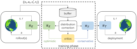
Following the philosophy of OAC and recent advances in the off-policy RL (Lee et al., 2021), we propose to simultaneously train a conservative target policy $\pi_{T}$ for deployment, and an optimistic exploration policy $\pi_{E}$ for executing the most informative actions w.r.t the current $Q$ value estimation. Figure 1 provides an overview of our framework. We apply explicit distribution corrections to train both policies and critics, and no constraint is imposed on $\pi_{E}$ in terms of its divergence from $\pi_{T}$.

In the rest of this section, we first introduce our off-policy training objectives and theoretically show that it forms an unbiased policy gradient estimator for $\pi_{T}$ with the distribution correction ratio. We then elaborate on how to estimate the distribution correction ratio by adapting the DICE optimization scheme. We close this section by summarizing our algorithm with pseudo-codes.

3.1 Off-policy Training Objectives

$\pi_{T}$ and $\pi_{E}$ are parameterized by $\theta_{T}$ and $\theta_{E}$ respectively. We start from the training objective for the target policy $\pi_{T}$. To prevent from overestimation, we follow previous work (Haarnoja et al., 2018; Fujimoto et al., 2018; Ciosek et al., 2019) in using the approximate lower bound $\hat{Q}_{\mathrm{LB}}$ as the critic, and correct the sample distribution with $\frac{d^{\pi_{T}}(s,a)}{d^{\mathcal{D}}(s,a)}$,

$$\hat{J}^{\pi_{T}}=\sum_{(s,a)\in\mathcal{D}}\frac{d^{\pi_{T}}(s,a)}{d^{\mathcal{D}}(s,a)}\big{(}\hat{Q}_{\mathrm{LB}}\left(s,f_{\theta_{T}}\left(s,\varepsilon\right)\right)-\alpha\log f_{\theta_{T}}\left(s,\varepsilon\right)\big{)}.$$ (5)

The following proposition (proved in the Appendix B) shows that the gradient of training objective (5) provides an unbiased estimation of the policy gradient (2). This contrasts with previous off-policy actor-critic algorithms that directly apply the biased estimator (3) in training the target policy.

Proposition 3.1.

$\nabla_{\theta_{T}}\hat{J}^{\pi_{T}}$ gives an unbiased estimate of the policy gradient (2) with $\pi=\pi_{T}$.

Regarding the exploration policy $\pi_{E}$, there are two considerations. Firstly, it should explore optimistically w.r.t. the estimated $Q$ values, in order to collect informative experience to efficiently correct spurious $Q$ estimates. Therefore, we follow OAC to use the approximate upper bound $\hat{Q}_{\mathrm{UB}}$ as critic in the objective. Secondly, the ultimate goal of $\pi_{E}$ and better $Q$ value estimation is to facilitate a more accurate gradient estimate for $\pi_{T}$. Therefore, the training sample distribution for $\pi_{E}$’s objective should be consistent with that for $\pi_{T}$’s. As a result, we apply the same correction ratio as in (5) to get the following objective for $\pi_{E}$,

$$\hat{J}^{\pi_{E}}=\sum_{(s,a)\in\mathcal{D}}\frac{d^{\pi_{T}}(s,a)}{d^{\mathcal{D}}(s,a)}\big{(}\hat{Q}_{\mathrm{UB}}\left(s,f_{\theta_{E}}\left(s,\varepsilon\right)\right)-\alpha\log f_{\theta_{E}}\left(s,\varepsilon\right)\big{)},$$ (6)

again, this is different from all existing works that adopt a separate exploration policy.

As for training the critics, while the best sample distribution for performing off-policy Q learning is still an open problem (Kumar et al., 2020), there exists some empirical work(Sinha et al., 2020; Nachum et al., 2019b) showing that using samples from the same distribution as that for policy training benefits the training of $Q$ functions. Therefore, we also apply the same correction ratio to $Q$ function objectives (1) and obtain the corrected objectives:

$$\hat{L}^{i}_{Q}=\sum_{(s,a)\in\mathcal{D}}\frac{d^{\pi_{T}}(s,a)}{d^{\mathcal{D}}(s,a)}\left(\hat{Q}_{i}(s,a)-\mathcal{B}^{\pi}\hat{Q}_{\mathrm{LB}}(s,a)\right)^{2}$$ (7)

3.2 Estimating Distribution Correction Ratio via DICE

We estimate the distribution correction ratio $\frac{d^{\pi_{T}}(s,a)}{d^{\mathcal{D}}(s,a)}$ by adapting the DICE optimization scheme (Yang et al., 2020). Yang et al. (2020) shows that existing DICE estimators can be formulated as the following min-max distributional linear program with different regularizations,

$$\max_{\zeta\geq 0}\min_{\nu,\lambda}\,\,L_{D}(\zeta,\nu,\lambda):= (1-\gamma)\cdot\mathbb{E}_{a_{0}\sim\pi_{T}\left(s_{0}\right)\atop s_{0}\in\rho_{0}(s)}\left[\nu\left(s_{0},a_{0}\right)\right]$$

$$+\lambda\cdot\left(1-\mathbb{E}_{\left(s,a,r,s^{\prime}\right)\sim d^{\mathcal{D}}}\left[\zeta(s,a)\right]\right)-\alpha_{\zeta}\cdot\mathbb{E}_{(s,a)\sim d^{\mathcal{D}}}\left[g_{2}(\zeta(s,a))\right]$$

$$+\mathbb{E}_{\left(s,a,r,s^{\prime}\right)\sim d^{\mathcal{D}}}\left[\zeta(s,a)\cdot\left(\mathcal{B}^{\pi_{T}}\nu(s,a)-\nu(s,a)\right)\right]$$

$$+\alpha_{\nu}\cdot\mathbb{E}_{(s,a)\sim d^{\mathcal{D}}}\left[g_{1}(\nu(s,a))\right],$$ (8)

where $g_{1}$ and $g_{2}$ are some convex and lower-semicontinuous regularization functions, $\alpha_{\nu}$ and $\alpha_{\zeta}$ control the corresponding regularization strength. By slightly abusing the notation, we define $\mathcal{B}^{\pi_{T}}\nu(s,a)=\alpha_{R}\cdot R(s,a)+\gamma\nu\left(s^{\prime},a^{\prime}\right),a^{\prime}\sim\pi_{T}(s^{\prime})$ with $\alpha_{R}$ scaling the reward. Solving the optimization problem (3.2) for $\zeta$ gives us $\zeta^{*}(s,a)=\frac{d^{\pi_{T}}(s,a)}{d^{\mathcal{D}}(s,a)}$, which is exactly the distribution correction ratio. Note that the formulation supports both discounted and undiscounted return cases.

We now provide intuitions for (3.2). For simplicity, we refer to RHS as the RHS of (3.2). As $\zeta^{*}(s,a)$ is the distribution correction ratio, $\lambda$ is the Lagrangian coefficient to ensure the expectation of $\zeta^{*}(s,a)$ to be $1$. $\nu$ can be viewed as a synonym to the $Q$, with the first line of the RHS giving the normalized expected per-step reward of policy $\pi_{T}$. Line 3 and 4 together can be viewed as the expected single-step bellman error, which becomes clear if referring to the Fenchel Duality and setting $g_{2}(\zeta)=\frac{1}{2}\zeta^{2}$. We refer interested readers to the original paper (Yang et al., 2020) for more details.

Directly applying the above DICE algorithms to the off-policy RL settings cast great optimization difficulties. While OPE assumes a fixed target policy and a static replay buffer with sufficient state-action space coverage (Nachum et al., 2019a), in RL, both the target policy and the replay buffer change during training. We thus make three modifications to (3.2) to overcome the challenges.

Our first modification to (3.2) is removing the $\mathbb{E}_{s_{0}\in\rho_{0}(s),a_{0}\sim\pi\left(s_{0}\right)}\left[\nu\left(s_{0},a_{0}\right)\right]$ term from the objective. In the initial training stage, the state-action pairs stored in the replay buffer only achieve little coverage of the entire state-action space, especially for high dimensional continuous control tasks. As a result, the target policy $\pi_{T}$ may sample some $a_{0}$ that is very different from any collected experience in the replay buffer. $\nu(s_{0},a_{0})$ will then be minimized pathologically low and thus incur a huge error. Note that similar phenomena also appear in the offline RL (Fujimoto et al., 2019; Kumar et al., 2019).

Our second modification is to add an absolute value operator $|\cdot|$ to the single step bellman error $\mathcal{B}^{\pi}\nu(s,a)-\nu(s,a)$. We empirically find that it increases the training stability. The intuition comes from considering solving for $L_{\zeta}$ defined by (11), since when $g_{2}$ is square function then the absolute value automatically helps the $\zeta$ function lie on the positive region without any hard projection.

Our third modification to the original problem (3.2) is to set both $\alpha_{\nu}$ and $\alpha_{\zeta}$ greater than zero. This is different from existing DICE schemes (Yang et al., 2020) that set either $\alpha_{\nu}$ or $\alpha_{\zeta}$ to be zero. Though such a setting introduces bias and has never been applied in existing DICE algorithms, it dramatically stabilizes the training in practice. Moreover, adding two regularizations on a min-max program has been widely applied for faster convergent in optimization literature (Allen-Zhu et al., 2016).

To this end, we obtain as follows the loss functions for each of $\nu$, $\zeta$, and $\lambda$ respectively,

$$L_{\lambda} =\lambda\cdot\left(1-\mathbb{E}_{\left(s,a,r,s^{\prime}\right)\sim d^{\mathcal{D}}}[\zeta(s,a)]\right),$$ (9)

$$L_{\nu} =\mathbb{E}_{\left(s,a,r,s^{\prime}\right)\sim d^{\mathcal{D}}}\left[\zeta(s,a)\cdot\left|\mathcal{B}^{\pi_{T}}\nu(s,a)-\nu(s,a)\right|\right]+\alpha_{\nu}\cdot\mathbb{E}_{(s,a)\sim d^{\mathcal{D}}}\left[g_{1}(\nu(s,a))\right],$$ (10)

$$L_{\zeta} =\alpha_{\zeta}\cdot\mathbb{E}_{(s,a)\sim d^{\mathcal{D}}}\left[g_{2}(\zeta(s,a))\right]-\mathbb{E}_{\left(s,a,r,s^{\prime}\right)\sim d^{\mathcal{D}}}\left[\zeta(s,a)\cdot\left(\left|\mathcal{B}^{\pi_{T}}\nu(s,a)-\nu(s,a)\right|-\lambda\right)\right].$$ (11)

Both $\zeta$ and $\nu$ are parameterized by neural networks with parameters $\eta_{\zeta}$ and $\eta_{\nu}$ respectively. To stabilize the training, we maintain a $\nu^{\prime}$ as the exponential moving average of $\nu$ to compute $\mathcal{B}^{\pi_{T}}\nu(s,a)$.

When applying the learned $\zeta(s,a)$ as a surrogate of $\frac{d^{\pi_{T}}(s,a)}{d^{\mathcal{D}}(s,a)}$ in the RL training objectives, we need to tackle the issue of finite samples since our training is in minibatch. Inspired by (Sinha et al., 2020), we apply self-normalization to $\zeta(s,a)$ with temperature $T$, and use the $\tilde{\zeta}(s,a)$ defined below to construct the RL objectives (5), (6) and (7).

$$\tilde{\zeta}(s,a)=\frac{\zeta(s,a)^{1/T}}{\sum_{(s,a)\sim\mathcal{D}}\zeta(s,a)^{1/T}}.$$ (12)

3.3 Summary of Algorithm

To this end, we summarize our overall algorithm in Algorithm 1. Like conventional off-policy actor-critic algorithms, we alternatively perform environment interactions following $\pi_{E}$ and update of all trainable parameters. In each training step, our algorithm first updates the $\nu$, $\zeta$, and $\lambda$ related to DICE, using SGD w.r.t. losses (10), (11), and (9) respectively, and computes the distribution correction ratio $\tilde{\zeta}$ from the updated $\zeta$. With $\tilde{\zeta}$, our algorithm then performs RL training to update $\pi_{T}$, $\pi_{E}$, $\hat{Q}_{1}$, and $\hat{Q}_{2}$. Finally, soft update of target critics $\hat{Q}^{\prime}_{1}$, $\hat{Q}^{\prime}_{2}$, and $\nu^{\prime}$ is performed

Algorithm 1 Optimistic Exploration with Explicit Distribution Correction

Input: target and explore policy parameters $\theta_{T}$, $\theta_{E}$; $\hat{Q}_{1}$, $\hat{Q}_{2}$ parameters $\omega_{1}$, $\omega_{2}$; $\hat{Q}^{\prime}_{1}$, $\hat{Q}^{\prime}_{2}$ parameters $\omega^{\prime}_{1}$, $\omega^{\prime}_{2}$; $\nu$, $\zeta$ parameters $\eta_{\nu}$, $\eta_{\zeta}$, $\nu^{\prime}$ parameters $\eta_{\nu^{\prime}}$, and $\lambda$; replay buffer $\mathcal{D}$

1:$w^{\prime}_{1}\leftarrow w_{1}$, $w^{\prime}_{2}\leftarrow w_{2}$, $\eta_{\nu^{\prime}}\leftarrow\eta_{\nu}$, $\mathcal{D}\leftarrow\emptyset$

2:repeat

3:     for each environment step do

4:         Sample action $a_{t}\sim\pi_{E}(\cdot|s_{t})$

5:         Observe $s_{t+1}\sim T(\cdot|s_{t},a_{T})$ and $r\left(\mathbf{s}_{t},\mathbf{a}_{t}\right)$

6:         $\mathcal{D}\leftarrow\mathcal{D}\cup\left\{\left(\mathbf{s}_{t},\mathbf{a}_{t},r\left(\mathbf{s}_{t},\mathbf{a}_{t}\right),\mathbf{s}_{t+1}\right)\right\}$

7:     end for

8:     for each training step do

9:         Sample minibatch $B=\{(s,a,r,s^{\prime})\}$ from $\mathcal{D}$

10:         # DICE training

11:         Update $\eta_{\nu}$, $\eta_{\zeta}$, $\lambda$ via $\nabla_{\eta_{\nu}}L_{\nu}$, $\nabla_{\eta_{\zeta}}L_{\zeta}$, $\nabla_{\psi_{\lambda}}L_{\lambda}$

12:         Calculate $\tilde{\zeta}$ with (12)

13:         # RL training

14:         Update $\theta_{T}$ with $\nabla_{\theta_{T}}\hat{J}^{\pi_{T}}$

15:         Update $\theta_{E}$ with $\nabla_{\theta_{E}}\hat{J}^{\pi_{E}}$

16:         Update $w_{i}$ with $\nabla_{w_{i}}\hat{L}^{i}_{Q}$, $i\in\{1,2\}$

17:         # Soft update

18:         $w^{\prime}_{i}\leftarrow\tau w_{i}+(1-\tau)w^{\prime}_{i}$, $i\in\{1,2\}$; $\eta_{\nu^{\prime}}\leftarrow\tau\eta_{\nu}+(1-\tau)\eta_{\nu^{\prime}}$

19:     end for

20:until convergence

4 Experimental Results

We validate the proposed algorithm from three perspectives. First, we compare our algorithm with SOTA off-policy actor-critic algorithms on challenging control tasks. Second, we examine the quality of our learned correction ratio by evaluating whether it helps to provide a reasonable estimate of the on-policy rewards. Third, we ablate key components of our algorithms to evaluate their contributions to the overall performance.

We evaluate on 5 continuous control tasks from the MuJoCo (Todorov et al., 2012) benchmark and compare it with SAC (Haarnoja et al., 2018) and OAC (Ciosek et al., 2019). We further implement a strong baseline OAC + DICE by integrating our DICE correction into OAC, i.e., similar to (5) and (7), using the learned distribution correction ratio to correct the sample distribution for both the target policy training and the critics training.

For each task, we run 5 different random seeds for each algorithm. We evaluate each algorithm every 1000 training steps. Our algorithm introduces additional hyper-parameters (HP), including $\beta_{\mathrm{LB}}$ and $\beta_{\mathrm{UB}}$ that control the extent of conservativeness and optimism respectively, the temperature $T$ from (7), and the set of hyper-parameters from the DICE optimization (9), (10), (11). We provide detailed hyper-parameter tuning procedures in the Appendix C. Note that the implementation of our algorithms are based on OAC’s officially released codes, which themselves are based on the SAC implementation in RLkit . While we are aware of different implementations of SAC with performance variance on different tasks, given the difficulty in reproducing the best RL results in practice (Engstrom et al., 2020; Pineau et al., 2021), we have tried our best to make all comparisons fair and reproducible by implementing all methods and variants in a unified and credible codebase.

4.1 Evaluation on Continuous Control Tasks

Figure 2: Our methods versus SAC, OAC, and the strong baseline OAC + DICE on 5 MuJoco tasks. x-axis indicates the number of environment steps. y-axis indicates the total undiscounted return. The shaded areas denote one standard deviation between 5 runs of different random seeds.

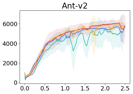
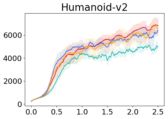
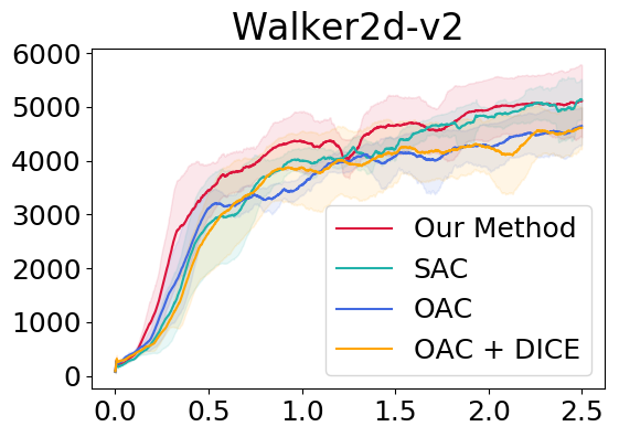
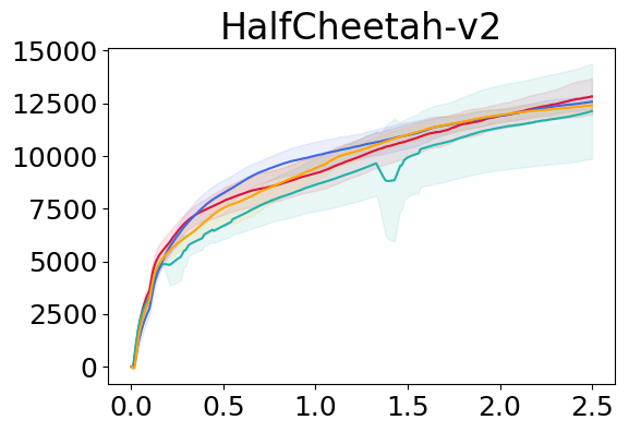
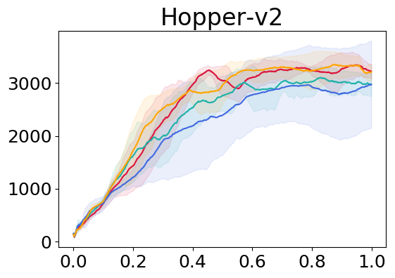
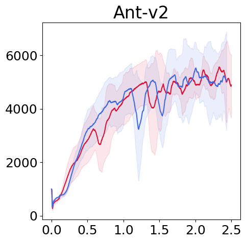
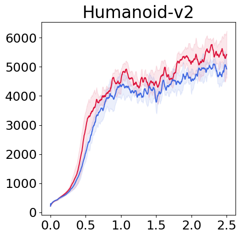
As shown in Figure 2, our method consistently outperforms both OAC and SAC on 4 out of the 5 tasks, while being on par with OAC on the less challenging HalfCheetah. The superior performance of our method vs OAC and SAC demonstrates the effectiveness of the proposed framework and the benefits of both the optimistic exploration and distribution correction for off-policy RL.

We would also like to highlight the performance of our specific baseline OAC + DICE. While it outperforms OAC by a large margin on Hopper, there are only slight improvements over OAC on Humanoid and Ant, even with no performance gain on Walker2d and HalfCheetah. These results demonstrate that the proposed distribution correction scheme at least does not harm the performance and often leads to improvements for off-policy actor-critic algorithms beyond ours. Moreover, the performance of our method vs. OAC + DICE on the more challenging Humanoid, Ant, and Walker2d demonstrates that our exploration policy design is superior to that of OAC when paired with the DICE distribution correction. This is not surprising. Due to the use of KL constraint in OAC, the actions generated by $\pi_{E}$ can not differ much from those generated by $\pi_{T}$ for most of the states. As a result, the potential of $\pi_{E}$ in collecting the most informative experience for correcting the critics has been largely constrained. Our method, on the other hand, does not impose any constraints on the distance between $\pi_{E}$ and $\pi_{T}$, and therefore learns a more effective exploration policy for collecting the informative experience for off-policy training.

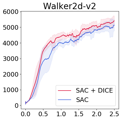
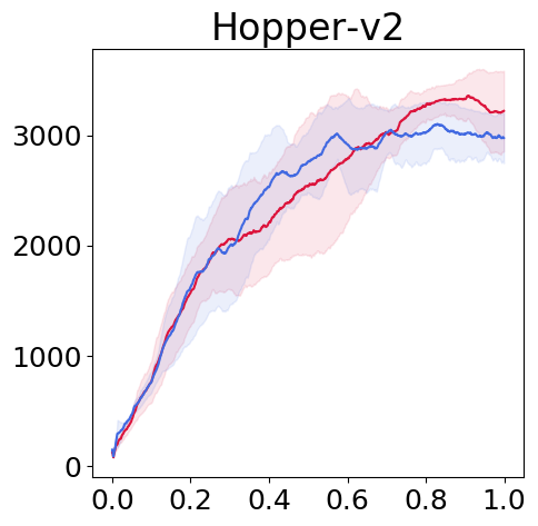
Similarly, we implement SAC + DICE by integrating our DICE correction ratio into SAC without any HP tuning. As shown in Figure 3, SAC + DICE outperforms SAC on the challenging Humanoid and Walker2d by a clear margin while being on par with SAC on the Ant. There is also a slight performance gain on the Hopper. It is worth noting that integrating our learned DICE correction ratio into NO DICE (a variant of ours), OAC, and SAC all results in a performance gain. We thus highlight that our proposed DICE correction scheme effectively benefits general off-policy actor-critic training.

Figure 3: Comparing SAC + DICE vs. SAC on 4 Mujoco environments. x-axis indicates the number of environment steps. y-axis indicates the total undiscounted return. The shaded areas denote one standard deviation between 5 runs of different random seeds.

4.2 Examine the Correction Ratio

Figure 4: Reward estimation results of our method (Our dual estimate), a naive baseline (Batch rewards), and a reference (On-policy rewards) on 5 Mujoco environments. x-axis is the number of environment steps. y-axis is the reward value. The shaded areas denote one standard deviation between 5 runs of different random seeds.

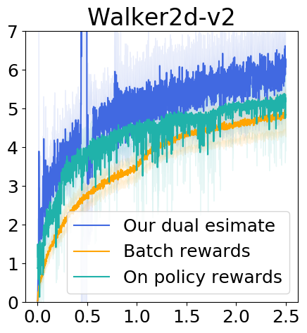
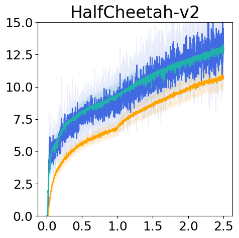
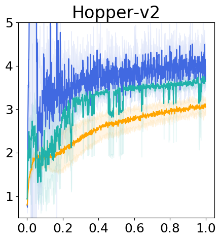
To examine the quality of the learned distribution correction ratio, we propose to tackle a novel OPE setting that is more challenging than the traditional counterpart, where both the target policy and the replay buffer are changing. Following our Algorithm 1 and the same experiment settings in Section 4.1, we now use the following dual estimator defined in (Yang et al., 2020) to estimate the on-policy average per-step rewards $r^{\pi_{T}}_{on}$ (on-policy rewards) of $\pi_{T}$,

$$\hat{\mu}_{\zeta}(\pi_{T})=\sum_{(s,a,r)\in\mathcal{D}}\zeta(s,a)r,$$ (13)

where $\zeta$ is the distribution correction ratio estimated in Algorithm 1. We use the metric $|\hat{\mu}_{\zeta}(\pi_{T})-r^{\pi_{T}}_{on}|$ to evaluate the OPE performance, which directly reflects the quality of $\zeta(s,a)$. If $|\hat{\mu}_{\zeta}(\pi)-r^{\pi_{T}}_{on}|<|r_{\mathcal{D}}-r^{\pi_{T}}_{on}|$, where $r_{\mathcal{D}}$ is the mean reward in the current replay buffer $\mathcal{D}$, correcting the training distribution of RL using the learned $\zeta$ can at least provide positive momentum to the overall training.

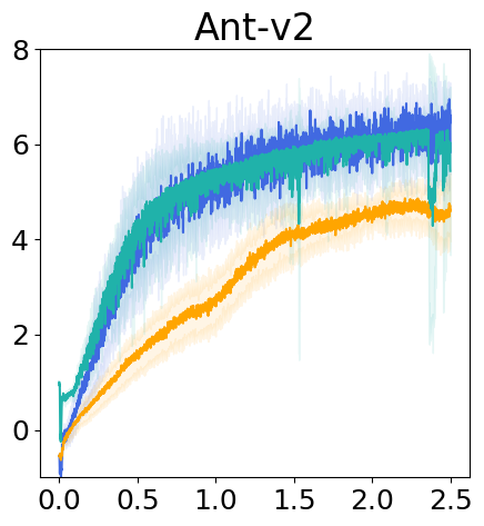
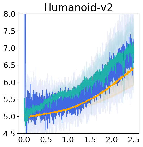
Figure 4 shows the performance of two OPE methods, i.e., “Our dual estimate" (13) and the naive “Batch rewards" baseline, both are estimated using a batch of transitions. We also plot the “on policy rewards" $r^{\pi_{T}}_{on}$ as a reference which averages over the rewards collected by the target policy during evaluation. As shown in Figure 4, our OPE performance is surprisingly decent. The $\hat{\mu}_{\zeta}(\pi)$ learned by our method nicely matches the on-policy reward estimate on Humanoid, Ant, and HalfCheetah, while staying close to the on-policy reward estimate on Hopper and Walker2d. These experimental results demonstrate the effectiveness of our adaptation of the DICE scheme from standard OPE to the off-policy RL setting, which also explains the success of our proposed algorithm in experiments of Section 4.1 where the power of this adapted DICE scheme has been leveraged.

4.3 Ablation Study

Figure 5: Ablation on our method on 5 Mujoco environments. x-axis indicates the number of environment steps. y-axis indicates the total undiscounted return. The shaded areas denote one standard deviation. Please zoom-in to see more details.

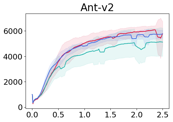
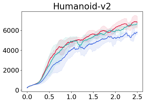
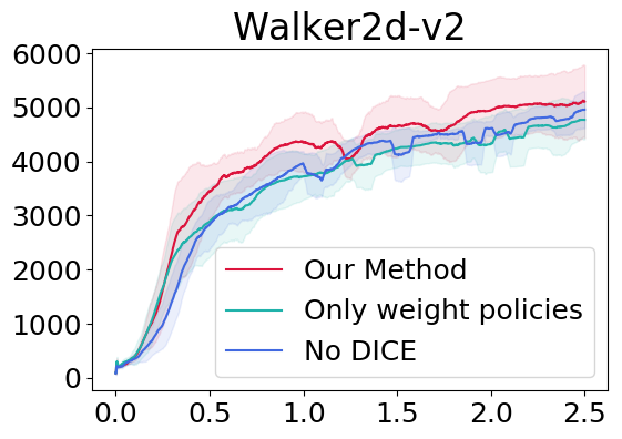
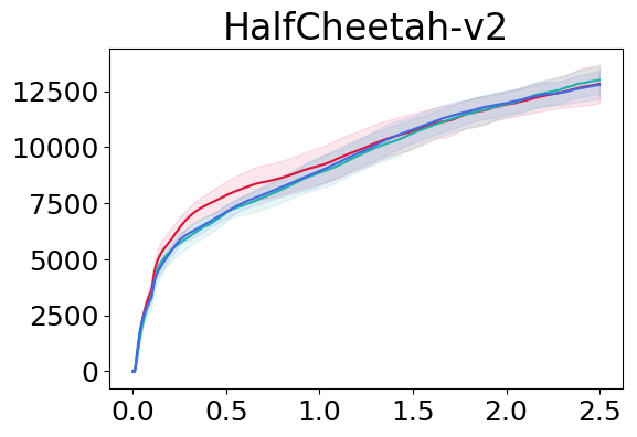
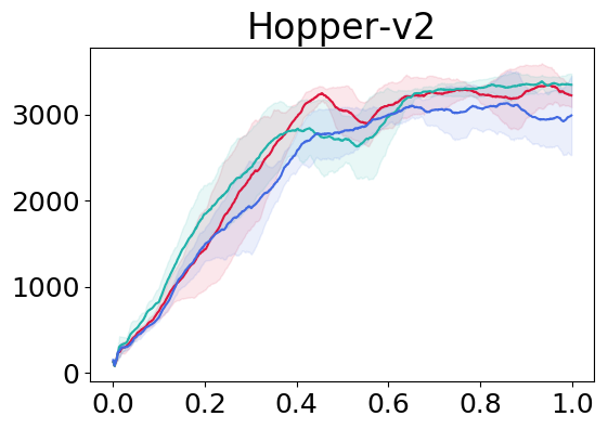
We emphasize the key of our framework is to explicitly correct the RL training distribution while training an explore policy solely to correct the flawed Q value that undermines the target policy’s gradient estimate. In Section 4.1, we already show that having such an exploration is beneficial. We now show by ablation that such an aggressive training strategy is indeed backed by our distribution correction techniques. The first ablated version of our method, No DICE, does not have the DICE component, i.e., its training procedures can be summarized as Algorithm 1 without Line 10-12, and always set $\tilde{\zeta}(s,a)=1$. As shown in Figure 5, the performance drops substantially on Humanoid, Walker2d, and Hopper, and somewhat on Ant and HalfCheetah, demonstrating the necessity of performing an effective distribution correction when applying an aggressive exploration strategy.

The second ablated version is to check the necessity of correcting the state-action distribution w.r.t the $Q$ function loss. We term the version of our method without applying the correction ratio to the $Q$ function objective as Only weight policies. From Figure 5, we can see the performance dropped dramatically on Ant and slightly on the other tasks. We include more ablation studies in the Appendix, showing how different HP influences the performance of our method.

5 Conclusion

In this paper, we proposed a novel off-policy RL paradigm that enables the training of an exploration policy that solely focuses on executing the most informative actions without constraining its divergence from the target policy. We support such an efficient exploration by learning the distribution correction ratio to correct the training distribution, which is realized by successfully adapting the DICE (Yang et al., 2020) optimization schemes into the off-policy actor-critic framework. By evaluating in challenging continuous control tasks, we demonstrate the effectiveness of our method.

Appendix

Outline of the Appendix

In this Appendix, we organize the content in the following ways:

• In Appendix A, we additional related works.

• In Appendix B, we present the proof of Proposition 3.1.

• In Appendix C, we present experiment details and hyper-parameter settings

• In Appendix D, we present additional ablation studies to examine how the hyper-parameters $\beta_{\mathrm{UB}}$, $\beta_{\mathrm{LB}}$ and $T$ impacts the performance. We also show the necessity of correcting the distribution of both the target and exploration policy objectives via comparing with another variant of our approach that only weights the Q function training.

Appendix A Additional Related Work

Incorporating the DICE family  [Nachum et al., 2019a, Zhang et al., 2020a, b, Uehara et al., 2020, Nachum and Dai, 2020, Nachum et al., 2019b, Yang et al., 2020] into the training process of off-policy actor-critic is never easy, as the DICE optimization itself already poses great optimization difficulties. Moreover, in RL, the target policy is always changing and remains unstable. When tackling complicated continuous control tasks with high dimensional state-action space, the instability gets even exacerbated by the limited state-action coverage at the initial training stage [Nachum et al., 2019a]. We tackle such difficulties by directly making modifications to the objectives and successfully stabilize the training. Though suffering from bias, experimental results show that our optimization objective actually leads to surprisingly good OPE performance.

In our work, by explicitly correcting the training distribution, we open up the direction to a potentially more profound exploration strategy design. There are a bunch of literature investigate to design better exploration objective  [Brafman and Tennenholtz, 2002, Kearns and Koller, 1999, Sorg et al., 2012, Lopes et al., 2012, Araya et al., 2012, Doshi-Velez et al., 2010]. While most of the pioneering works mainly tackle the problem in discrete or small state-action space via directly operate on the transition matrix, which cannot be directly extended to complicated continuous control tasks. Noise-based methods [Fortunato et al., 2017, Plappert et al., 2017] improve exploration by perturbing the observation, state, or the parameters in the function approximator for obtaining diverse actions. Intrinsic motivation has also been introduced to encourage the agent to discover novel states [Pathak et al., 2017, Burda et al., 2018a, Stadie et al., 2015, Tang et al., 2017, Pathak et al., 2019] or better understand the environment [Houthooft et al., 2016, Zhao and Tresp, 2019, Burda et al., 2018b, Savinov et al., 2018, Choshen et al., 2018, Denil et al., 2016]. Inspired by Thompson sampling, Osband et al.[Osband et al., 2016] propose to improve exploration of DQN [Mnih et al., 2013] by modeling uncertainty. Eysenbach et al.[Eysenbach et al., 2018] propose to encourage exploration through maximizing the diversity of the learned behavior. SAC [Haarnoja et al., 2018] tries to improve exploration through adding extra regularization on the entropy term, while OAC [Ciosek et al., 2019] derives an upper confidence bound on the state-action value function for facilitating exploration. Although these methods demonstrate that good exploration will benefit the learning process, these works neglect the issue of distribution shift and instability, which is also proven to be a non-trival problem in reinforcement learning [Kumar et al., 2020, Sinha et al., 2020].

Appendix B Proof of Proposition 3.1

Proposition 3.1. $\nabla_{\theta_{T}}\hat{J}^{\pi_{T}}$ gives an unbiased estimate of the policy gradient (2) with $\pi=\pi_{T}$.

Proof.

Recall that

$$\nabla_{\theta}J^{\pi}=\int_{s}d^{\pi}(s)\bigg{(}\int_{\varepsilon}\nabla_{\theta}\hat{Q}_{\mathrm{LB}}\left(s,f_{\theta}(s,\varepsilon)\right)\phi(\varepsilon)d\varepsilon+\alpha\int_{\varepsilon}-\nabla_{\theta}\log f_{\theta}(s,\varepsilon)\phi(\varepsilon)d\varepsilon\bigg{)}ds$$

$$\hat{J}^{\pi_{T}}=\sum_{(s,a)\in\mathcal{D}}\frac{d^{\pi_{T}}(s,a)}{d^{\mathcal{D}}(s,a)}\big{(}\hat{Q}_{\mathrm{LB}}\left(s,f_{\theta_{T}}\left(s,\varepsilon\right)\right)-\alpha\log f_{\theta_{T}}\left(s,\varepsilon\right)\big{)}.$$

Therefore, $\nabla_{\theta_{T}}\hat{J}^{\pi_{T}}$ is an unbiased estimator for

$$\quad\int_{s}\int_{a}d^{\mathcal{D}}(s,a)\frac{d^{\pi_{T}}(s,a)}{d^{\mathcal{D}}(s,a)}\left(\int_{\varepsilon}\nabla_{\theta_{T}}\left(\hat{Q}_{\mathrm{LB}}\left(s,f_{\theta_{T}}(s,\varepsilon)\right)-\alpha\log f_{\theta_{T}}(s,\varepsilon)\right)\phi(\varepsilon)d\varepsilon\right)dads$$

$$=\int_{s}\int_{a}d^{\pi_{T}}(s,a)\left(\int_{\varepsilon}\nabla_{\theta_{T}}\left(\hat{Q}_{\mathrm{LB}}\left(s,f_{\theta_{T}}(s,\varepsilon)\right)-\alpha\log f_{\theta_{T}}(s,\varepsilon)\right)\phi(\varepsilon)d\varepsilon\right)dads$$

$$=\int_{s}d^{\pi_{T}}(s)\left(\int_{\varepsilon}\nabla_{\theta_{T}}\left(\hat{Q}_{\mathrm{LB}}\left(s,f_{\theta_{T}}(s,\varepsilon)\right)-\alpha\log f_{\theta_{T}}(s,\varepsilon)\right)\phi(\varepsilon)d\varepsilon\right)ds=\nabla_{\theta_{T}}J^{\pi_{T}}$$

∎

Appendix C Hyper-parameters (HP) and Experiment Details

The implementation of our method is based on OAC’s officially released codes, which themselves are based on the SAC implementation in RLkit . We are aware of the fact that OAC’s officially released codes${}^{\ref{oac}}$ use a set of HP that is slightly different from its original paper. Specifically, they set $\beta_{\mathrm{LB}}=1.0$ instead of $3.65$ as per (Table 1, Appendix E) of OAC’s original paper [Ciosek et al., 2019].

The implementation to solve the DICE optimization is based on the official dice_rl repo. We set the regularization function $g_{1}(x)=g_{2}(x)=\frac{1}{m}|x|^{m}$ in Equation (10) and (11), where we treat the exponential $p$ as a hyper-parameter. All of our results are obtained by averaging across $5$ fixed random seeds as per Appendix D of OAC’s original paper [Ciosek et al., 2019].

We list the HP specific to our method and those different from SAC and OAC in Table 1. For completeness, we include the HP for SAC and OAC${}^{\ref{oac}}$ in Table 2. We set both $\alpha_{\nu}=1$ and $\alpha_{\zeta}=1$ as we found this is the only setting to stabilize the DICE optimization in our HP space. We set the temperature $T=3.0$ as our preliminary experiment finds the value of $T$ from our HP space will not significantly impact the performance, which is proved in our ablation study (Appendix D.1). As for $\beta_{\mathrm{UB}}$ and $\beta_{\mathrm{LB}}$, we tune their values simultaneously. However, we do not conduct the full sweep in the HP space due to limited computational resources. We empirically find it beneficial to set a similar value for $\beta_{\mathrm{UB}}$ and $\beta_{\mathrm{LB}}$ (Appendix D.2).

Table 1: Hyper-parameters of our method

Hyper-parameters	Value	Range used for tuning
$\beta_{\mathrm{UB}}$	2.0	$\{1.5,2.0,2.5,3.0\}$
$\beta_{\mathrm{LB}}$	2.5	$\{1.5,2.0,2.5,3.0\}$
Temperature $T$	3.0	{2.0, 3.0, 5.0}
Learning rate for $\nu,\zeta,\lambda$	0.0001	Does not tune
$\alpha_{\nu}$	1	{0, 1}
$\alpha_{\zeta}$	1	{0, 1}
discount($\gamma$) for DICE	0.99	Does not tune
Regularization function exponential $m$	1.5	Does not tune
$\nu,\zeta$ network hidden sizes	[256, 256]	Does not tune
$\nu,\zeta,\lambda$ optimizer	Adam [Kingma and Ba, 2014]	Does not tune
$\nu,\zeta$ network nonlinearity	ReLU	Does not tune

Table 2: Hyper-parameters of SAC and OAC${}^{\ref{oac}}$

Parameter	Value
policy and $Q$ optimizer	Adam [Kingma and Ba, 2014]
learning rate for policy and Q	$3\cdot 10^{-4}$
discount($\gamma$)	0.99
replay buffer size	$10^{6}$
policy and $Q$ network hidden sizes	[256, 256]
minibatch size	256
policy and $Q$ nonlinearity	ReLU
target smoothing rate($\tau$)	0.005
target update interval	1
gradient steps	1
OAC-specific Parameter	Value
shift multiplier $\sqrt{2\delta}$	6.86
$\beta_{\mathrm{UB}}$	4.66
$\beta_{\mathrm{LB}}$	1.0

Appendix D Additional Ablation Study

D.1 Ablation study of the temperature $T$

Figure 6: Ablation study on the temperature $T$ of our method on 4 Mujoco environments. x-axis indicates the number of environment steps and y-axis indicates the total undiscounted return. The shaded areas denote one standard deviation between 5 runs of different random seeds.

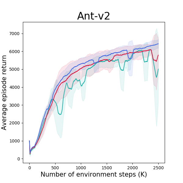
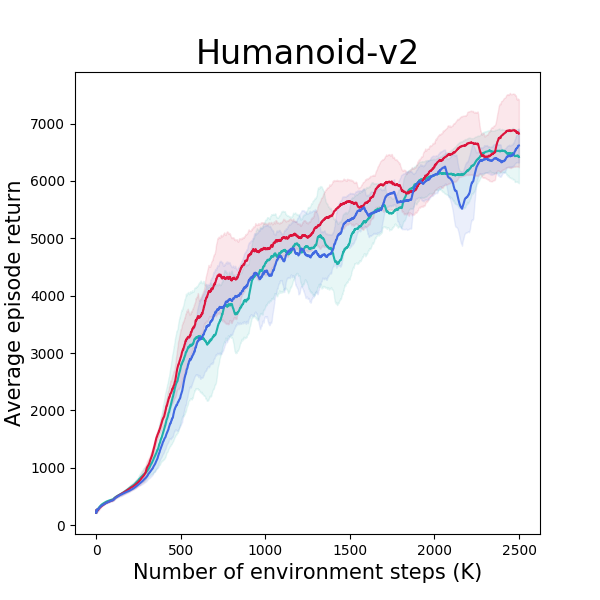
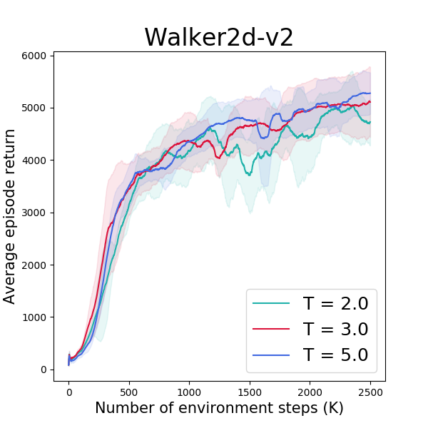
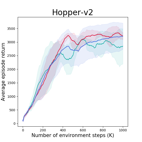
In this section, we examine how the temperature $T$ influences the performance. Note that we keep the other HP unchanged as per Table 1. For $T\in\{2.0,3.0,5.0\}$, we present the performance of Our Method on 4 MuJoCo tasks as shown in Figure 6. A low value of $T$ will introduce instability to the training process, especially for Ant and Walker2d, while the performance on Humanoid remains stable w.r.t different $T$. With $T\geq 3.0$, we can achieve a stable training process and decent final performance in all 4 tasks.

D.2 Ablation study of $\beta_{\mathrm{UB}}$ and $\beta_{\mathrm{LB}}$

Figure 7: Ablation study on the $\beta_{\mathrm{UB}},\beta_{\mathrm{LB}}$ of our method on 4 MuJoco tasks. x-axis indicates the number of environment steps. y-axis indicates the total undiscounted return. The shaded areas denote one standard deviation between 5 runs of different random seeds.

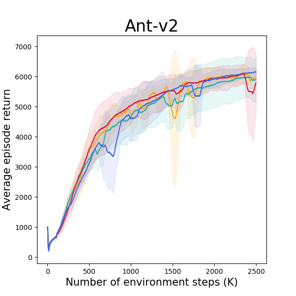
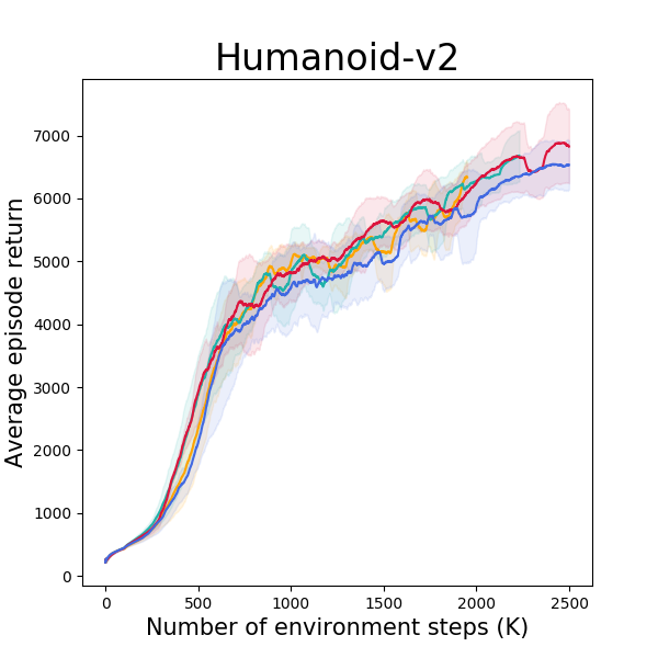
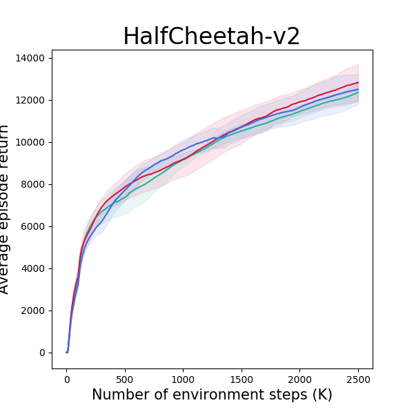
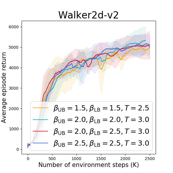
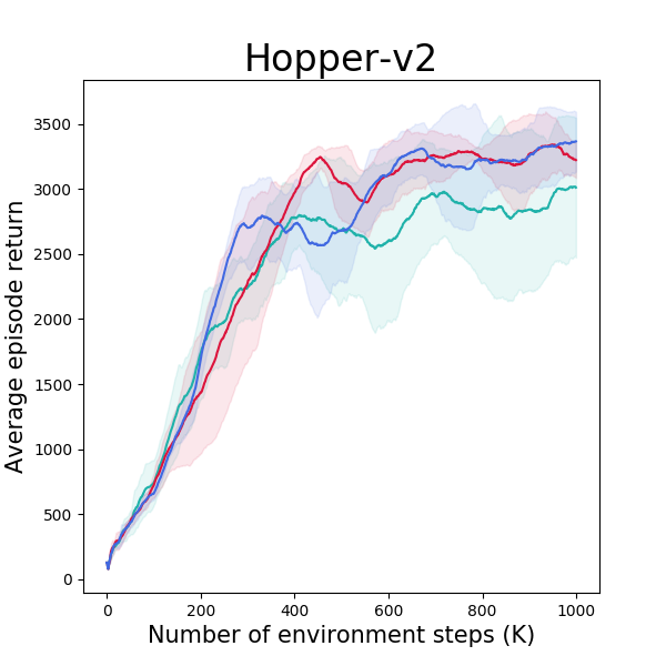
In this section, we examine how different values of $\beta_{\mathrm{UB}}$ and $\beta_{\mathrm{LB}}$ influence the performance of our method. We empirically find that setting similar values to $\beta_{\mathrm{UB}}$ and $\beta_{\mathrm{LB}}$ generally lead to good performance.

Note that the performance of $\beta_{\mathrm{UB}}=1.5$, $\beta_{\mathrm{LB}}=1.5$, and $T=2.5$ is to show that Our Method is robust to a wide range of $\beta_{\mathrm{UB}}$ and $\beta_{\mathrm{LB}}$ beyonds $\{2.0,2.5\}$.

D.3 Ablations on correcting the training distributions of the policies

Figure 8: Ablation study on correcting the training distributions of the policies on 2 MuJoCo tasks. x-axis indicates the number of environment steps. y-axis indicates the total undiscounted return. The shaded areas denote one standard deviation between 5 runs of different random seeds.

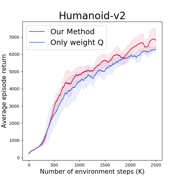
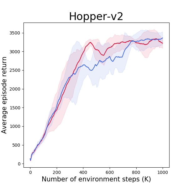
Similar to Only weight policies, we construct the ablated version of our method Only weight Q by removing the distribution correction applied to the target policy’s objective (5) and exploration policy’s objective (6). As shown in Figure 8, ablating the distribution correction for both target and exploration policies of Our Method leads to a clear performance loss on Humanoid. And the ablated version of Our Method also converges slower on the Hopper. Therefore, we can conclude that it is necessary to correct the training distributions of the target and exploration policy.

References

- Mnih et al. [2013] Volodymyr Mnih, Koray Kavukcuoglu, David Silver, Alex Graves, Ioannis Antonoglou, Daan Wierstra, and Martin Riedmiller. Playing atari with deep reinforcement learning. arXiv preprint arXiv:1312.5602, 2013.
- Silver et al. [2016] David Silver, Aja Huang, Chris J Maddison, Arthur Guez, Laurent Sifre, George Van Den Driessche, Julian Schrittwieser, Ioannis Antonoglou, Veda Panneershelvam, Marc Lanctot, et al. Mastering the game of go with deep neural networks and tree search. nature, 529(7587):484–489, 2016.
- Kalashnikov et al. [2018] Dmitry Kalashnikov, Alex Irpan, Peter Pastor, Julian Ibarz, Alexander Herzog, Eric Jang, Deirdre Quillen, Ethan Holly, Mrinal Kalakrishnan, Vincent Vanhoucke, et al. Qt-opt: Scalable deep reinforcement learning for vision-based robotic manipulation. arXiv preprint arXiv:1806.10293, 2018.
- Shani et al. [2005] Guy Shani, David Heckerman, Ronen I Brafman, and Craig Boutilier. An mdp-based recommender system. Journal of Machine Learning Research, 6(9), 2005.
- Li et al. [2019] Jiachen Li, Quan Vuong, Shuang Liu, Minghua Liu, Kamil Ciosek, Keith Ross, Henrik Iskov Christensen, and Hao Su. Multi-task batch reinforcement learning with metric learning. arXiv preprint arXiv:1909.11373, 2019.
- Degris et al. [2012] Thomas Degris, Martha White, and Richard S Sutton. Off-policy actor-critic. arXiv preprint arXiv:1205.4839, 2012.
- Haarnoja et al. [2018] Tuomas Haarnoja, Aurick Zhou, Pieter Abbeel, and Sergey Levine. Soft actor-critic: Off-policy maximum entropy deep reinforcement learning with a stochastic actor. arXiv preprint arXiv:1801.01290, 2018.
- Fujimoto et al. [2018] Scott Fujimoto, Herke van Hoof, and David Meger. Addressing function approximation error in actor-critic methods. CoRR, abs/1802.09477, 2018. URL http://arxiv.org/abs/1802.09477.
- Lillicrap et al. [2015] Timothy P Lillicrap, Jonathan J Hunt, Alexander Pritzel, Nicolas Heess, Tom Erez, Yuval Tassa, David Silver, and Daan Wierstra. Continuous control with deep reinforcement learning. arXiv preprint arXiv:1509.02971, 2015.
- Sutton and Barto [2018] Richard S Sutton and Andrew G Barto. Reinforcement learning: An introduction. MIT press, 2018.
- Van Hasselt et al. [2018] Hado Van Hasselt, Yotam Doron, Florian Strub, Matteo Hessel, Nicolas Sonnerat, and Joseph Modayil. Deep reinforcement learning and the deadly triad. arXiv preprint arXiv:1812.02648, 2018.
- Auer et al. [2002] Peter Auer, Nicolo Cesa-Bianchi, and Paul Fischer. Finite-time analysis of the multiarmed bandit problem. Machine learning, 47(2):235–256, 2002.
- Jin et al. [2020] Chi Jin, Zhuoran Yang, Zhaoran Wang, and Michael I Jordan. Provably efficient reinforcement learning with linear function approximation. In Conference on Learning Theory, pages 2137–2143. PMLR, 2020.
- Precup et al. [2001] Doina Precup, Richard S Sutton, and Sanjoy Dasgupta. Off-policy temporal-difference learning with function approximation. In ICML, pages 417–424, 2001.
- Nachum et al. [2019a] Ofir Nachum, Yinlam Chow, Bo Dai, and Lihong Li. Dualdice: Behavior-agnostic estimation of discounted stationary distribution corrections. arXiv preprint arXiv:1906.04733, 2019a.
- Nachum et al. [2019b] Ofir Nachum, Bo Dai, Ilya Kostrikov, Yinlam Chow, Lihong Li, and Dale Schuurmans. Algaedice: Policy gradient from arbitrary experience. arXiv preprint arXiv:1912.02074, 2019b.
- Zhang et al. [2020a] Ruiyi Zhang, Bo Dai, Lihong Li, and Dale Schuurmans. Gendice: Generalized offline estimation of stationary values. arXiv preprint arXiv:2002.09072, 2020a.
- Zhang et al. [2020b] Shangtong Zhang, Bo Liu, and Shimon Whiteson. Gradientdice: Rethinking generalized offline estimation of stationary values. In International Conference on Machine Learning, pages 11194–11203. PMLR, 2020b.
- Uehara et al. [2020] Masatoshi Uehara, Jiawei Huang, and Nan Jiang. Minimax weight and q-function learning for off-policy evaluation. In International Conference on Machine Learning, pages 9659–9668. PMLR, 2020.
- Yang et al. [2020] Mengjiao Yang, Ofir Nachum, Bo Dai, Lihong Li, and Dale Schuurmans. Off-policy evaluation via the regularized lagrangian. arXiv preprint arXiv:2007.03438, 2020.
- Kingma and Welling [2013] Diederik P Kingma and Max Welling. Auto-encoding variational bayes. arXiv preprint arXiv:1312.6114, 2013.
- Ciosek et al. [2019] Kamil Ciosek, Quan Vuong, Robert Loftin, and Katja Hofmann. Better exploration with optimistic actor-critic. arXiv preprint arXiv:1910.12807, 2019.
- Nachum and Dai [2020] Ofir Nachum and Bo Dai. Reinforcement learning via fenchel-rockafellar duality. arXiv preprint arXiv:2001.01866, 2020.
- Lee et al. [2021] Kimin Lee, Michael Laskin, Aravind Srinivas, and Pieter Abbeel. Sunrise: A simple unified framework for ensemble learning in deep reinforcement learning. In International Conference on Machine Learning, pages 6131–6141. PMLR, 2021.
- Kumar et al. [2020] Aviral Kumar, Abhishek Gupta, and Sergey Levine. Discor: Corrective feedback in reinforcement learning via distribution correction. arXiv preprint arXiv:2003.07305, 2020.
- Sinha et al. [2020] Samarth Sinha, Jiaming Song, Animesh Garg, and Stefano Ermon. Experience replay with likelihood-free importance weights. arXiv preprint arXiv:2006.13169, 2020.
- Fujimoto et al. [2019] Scott Fujimoto, David Meger, and Doina Precup. Off-policy deep reinforcement learning without exploration. In International Conference on Machine Learning, pages 2052–2062, 2019.
- Kumar et al. [2019] Aviral Kumar, Justin Fu, Matthew Soh, George Tucker, and Sergey Levine. Stabilizing off-policy q-learning via bootstrapping error reduction. In Advances in Neural Information Processing Systems, pages 11761–11771, 2019.
- Allen-Zhu et al. [2016] Zeyuan Allen-Zhu, Zhenyu Liao, and Yang Yuan. Optimization Algorithms for Faster Computational Geometry. In Ioannis Chatzigiannakis, Michael Mitzenmacher, Yuval Rabani, and Davide Sangiorgi, editors, 43rd International Colloquium on Automata, Languages, and Programming (ICALP 2016), volume 55 of Leibniz International Proceedings in Informatics (LIPIcs), pages 53:1–53:6, Dagstuhl, Germany, 2016. Schloss Dagstuhl–Leibniz-Zentrum fuer Informatik. ISBN 978-3-95977-013-2. doi: 10.4230/LIPIcs.ICALP.2016.53. URL http://drops.dagstuhl.de/opus/volltexte/2016/6332.
- Todorov et al. [2012] Emanuel Todorov, Tom Erez, and Yuval Tassa. Mujoco: A physics engine for model-based control. In 2012 IEEE/RSJ International Conference on Intelligent Robots and Systems, pages 5026–5033. IEEE, 2012.
- Engstrom et al. [2020] Logan Engstrom, Andrew Ilyas, Shibani Santurkar, Dimitris Tsipras, Firdaus Janoos, Larry Rudolph, and Aleksander Madry. Implementation matters in deep policy gradients: A case study on ppo and trpo. arXiv preprint arXiv:2005.12729, 2020.
- Pineau et al. [2021] Joelle Pineau, Philippe Vincent-Lamarre, Koustuv Sinha, Vincent Larivière, Alina Beygelzimer, Florence d’Alché Buc, Emily Fox, and Hugo Larochelle. Improving reproducibility in machine learning research (a report from the neurips 2019 reproducibility program). Journal of Machine Learning Research, 22, 2021.
- Brafman and Tennenholtz [2002] Ronen I Brafman and Moshe Tennenholtz. R-max-a general polynomial time algorithm for near-optimal reinforcement learning. Journal of Machine Learning Research, 3(Oct):213–231, 2002.
- Kearns and Koller [1999] Michael Kearns and Daphne Koller. Efficient reinforcement learning in factored mdps. In IJCAI, volume 16, pages 740–747, 1999.
- Sorg et al. [2012] Jonathan Sorg, Satinder Singh, and Richard L Lewis. Variance-based rewards for approximate bayesian reinforcement learning. arXiv preprint arXiv:1203.3518, 2012.
- Lopes et al. [2012] Manuel Lopes, Tobias Lang, Marc Toussaint, and Pierre-Yves Oudeyer. Exploration in model-based reinforcement learning by empirically estimating learning progress. In Neural Information Processing Systems (NIPS), 2012.
- Araya et al. [2012] Mauricio Araya, Olivier Buffet, and Vincent Thomas. Near-optimal brl using optimistic local transitions. arXiv preprint arXiv:1206.4613, 2012.
- Doshi-Velez et al. [2010] Finale Doshi-Velez, David Wingate, Nicholas Roy, and Joshua Tenenbaum. Nonparametric bayesian policy priors for reinforcement learning. 2010.
- Fortunato et al. [2017] Meire Fortunato, Mohammad Gheshlaghi Azar, Bilal Piot, Jacob Menick, Ian Osband, Alex Graves, Vlad Mnih, Remi Munos, Demis Hassabis, Olivier Pietquin, et al. Noisy networks for exploration. arXiv preprint arXiv:1706.10295, 2017.
- Plappert et al. [2017] Matthias Plappert, Rein Houthooft, Prafulla Dhariwal, Szymon Sidor, Richard Y Chen, Xi Chen, Tamim Asfour, Pieter Abbeel, and Marcin Andrychowicz. Parameter space noise for exploration. arXiv preprint arXiv:1706.01905, 2017.
- Pathak et al. [2017] Deepak Pathak, Pulkit Agrawal, Alexei A Efros, and Trevor Darrell. Curiosity-driven exploration by self-supervised prediction. In International conference on machine learning, pages 2778–2787. PMLR, 2017.
- Burda et al. [2018a] Yuri Burda, Harri Edwards, Deepak Pathak, Amos Storkey, Trevor Darrell, and Alexei A Efros. Large-scale study of curiosity-driven learning. arXiv preprint arXiv:1808.04355, 2018a.
- Stadie et al. [2015] Bradly C Stadie, Sergey Levine, and Pieter Abbeel. Incentivizing exploration in reinforcement learning with deep predictive models. arXiv preprint arXiv:1507.00814, 2015.
- Tang et al. [2017] Haoran Tang, Rein Houthooft, Davis Foote, Adam Stooke, Xi Chen, Yan Duan, John Schulman, Filip De Turck, and Pieter Abbeel. # exploration: A study of count-based exploration for deep reinforcement learning. In 31st Conference on Neural Information Processing Systems (NIPS), volume 30, pages 1–18, 2017.
- Pathak et al. [2019] Deepak Pathak, Dhiraj Gandhi, and Abhinav Gupta. Self-supervised exploration via disagreement. In International conference on machine learning, pages 5062–5071. PMLR, 2019.
- Houthooft et al. [2016] Rein Houthooft, Xi Chen, Yan Duan, John Schulman, Filip De Turck, and Pieter Abbeel. Vime: Variational information maximizing exploration. arXiv preprint arXiv:1605.09674, 2016.
- Zhao and Tresp [2019] Rui Zhao and Volker Tresp. Curiosity-driven experience prioritization via density estimation. arXiv preprint arXiv:1902.08039, 2019.
- Burda et al. [2018b] Yuri Burda, Harrison Edwards, Amos Storkey, and Oleg Klimov. Exploration by random network distillation. arXiv preprint arXiv:1810.12894, 2018b.
- Savinov et al. [2018] Nikolay Savinov, Anton Raichuk, Raphaël Marinier, Damien Vincent, Marc Pollefeys, Timothy Lillicrap, and Sylvain Gelly. Episodic curiosity through reachability. arXiv preprint arXiv:1810.02274, 2018.
- Choshen et al. [2018] Leshem Choshen, Lior Fox, and Yonatan Loewenstein. Dora the explorer: Directed outreaching reinforcement action-selection. arXiv preprint arXiv:1804.04012, 2018.
- Denil et al. [2016] Misha Denil, Pulkit Agrawal, Tejas D Kulkarni, Tom Erez, Peter Battaglia, and Nando De Freitas. Learning to perform physics experiments via deep reinforcement learning. arXiv preprint arXiv:1611.01843, 2016.
- Osband et al. [2016] Ian Osband, Charles Blundell, Alexander Pritzel, and Benjamin Van Roy. Deep exploration via bootstrapped dqn. Advances in neural information processing systems, 29:4026–4034, 2016.
- Eysenbach et al. [2018] Benjamin Eysenbach, Abhishek Gupta, Julian Ibarz, and Sergey Levine. Diversity is all you need: Learning skills without a reward function. arXiv preprint arXiv:1802.06070, 2018.
- Kingma and Ba [2014] Diederik P Kingma and Jimmy Ba. Adam: A method for stochastic optimization. arXiv preprint arXiv:1412.6980, 2014.