Problems of Position Reconstruction in Silicon Microstrip Detectors

Gregorio Landi
Dipartimento di Fisica e Astronomia, Universita’ di Firenze and INFN, Sezione di Firenze,
Largo E. Fermi 2 (Arcetri) 50125, Firenze, Italy

October 20, 2021 and August 11, 2005
Corresponding author. Gregorio.Landi@fi.infn.it
Abstract

The algorithms for position reconstruction in silicon micro-strip detectors are studied, and the signals of a minimum ionizing particle are simulated. The center-of-gravity distributions of the data events allow the fine tuning of the signal forms and of the strip response functions. In the sensors with floating strips the response function turns out to roughly approximate the response of a triangular function for the size of the signal involved. The simulations are extended to non orthogonal incidence. In these directions, and in general for all the asymmetric signal distributions, the standard application of the Ξ·πœ‚\eta algorithm introduces a systematic error. A signal reconstruction theorem gives the way to implement the corrections of this error.

Keywords: Center of gravity, Ξ·πœ‚\eta-algorithm, Position reconstructions, Silicon detectors.

1 Introduction 2021

Position reconstructions for a special type of silicon micro-strip detectors were the argument of this work. This type of double-sided micro-strip detectors was developed for the ALEPH vertex detector, and installed also in the L3 micro-vertex detector. However, during our participation to the L3 experiment, our attention was attracted by the track reconstruction in the L3 central chambers using the spin glass theory. The definition of a spin, required the sole hit positions, thus, the properties of the signals produced by the micro-strip detectors were completely neglected. Also the developments of refs.Β [1, 2] were conceived principally for electromagnetic calorimeters, only marginally devoted the silicon trackers. However, the availability of a sample of test beam data of those double sided detectors (for the PAMELA experiment) raised our interest for an application of the methods of ref.Β [1]. Though, some new developments were necessary, the limitation of the Ξ·πœ‚\eta-algorithm to symmetric systems came in immediate evidence. The initial constant of the algorithm could be easily selected only in special cases (i.e. for orthogonal incidence without magnetic field). The recommendations of ref.Β [5], of an use for symmetric systems, was completely neglected in the implementation of the algorithm in data analysis of running experiments. The warning about this point probably originates few abandons of the Ξ·πœ‚\eta-algorithm in favor of the simpler center of gravity. Instead, a careful study of the simulations gave us an hint to demonstrate a first method of correcting this systematic error in absence of magnetic field.

The efficacy of the method was tested in a dedicated test beam (PoS(Vertex 2007) 048) with excellent results. Other more sophisticated methods were developed to correct the algorithm also for moderate magnetic fields. A better and simpler method was found as a by-product of an advanced method of track reconstruction. In fact, the observation of anomalies in the distributions of errors in some of the following scatter-plots (figure 11 for example) evidenced the impossibility of an identical variance for the hit errors (a standard assumption of all the books on mathematical statistics) and triggered a deep search for realistic models of the error distributions of the observations. These realistic probabilities, turn out to be different for each hit. As expected for the Landau distribution of charge released. The realistic probabilities allowed substantial increases of the resolution for the track estimators. The developments, in the following, were essential for those advanced tasks, supported also by theorems that impose the account of the hit differences for optimal fits ( arXiv:2103.03464 and therein references).

The two-columns printing of Nuclear Instruments and Methods in Physics Research (A 554 2005 226) introduced few typing errors, undetected by our proof revision, absent in this version.

2 Introduction

The aim of this work is an application of the developments of ref.Β [1] andΒ [2] to the position reconstruction algorithms for silicon microstrip detectors. This application turns out somewhat complex and probably too detailed for the huge amount of data expected by future high energy experiments. But, in some experiments, the alignment parameters of the detector components are obtained through the position reconstruction algorithms. It is evident the need of maximum precision in these calibrations.

The detectors we are interested in are double sided silicon sensors of the type used in ALEPHΒ [3] and L3Β [4]: one side has all the strips connected to the electronics, the other side has one strip each two connected to the electronics. The unconnected strips are called "floating strips".

The first step is the simulation of the signals released in the sensor by a minimum ionizing particle (MIP). Our simulations are intended to be realistic enough to allow a non trivial exploration of the position reconstruction properties for non orthogonal incidences of a MIP. The fact that the strip charge collection works as a powerful low pass filter assures that few parameters are really important. To select them, we will use in reverse mode the properties of the position reconstruction algorithms.

We proved in ref.Β [1] the strict connection of the center of gravity (COG) algorithm with the Fourier Transform (FT) of the signal collected. Thus, our first task will be the calculation of the charge distribution (and its FT) that arrives to the collecting electrodes. The signal shapes we will explore are average signals; the fluctuations of the energy release and of its diffusion are different in each event, but their averages are supposed well defined. Section 2 is devoted to the determination of the FT of the signals integrated by the strips. A parameter is left free and extracted from the data

In the sections 3 and 4, the experimental data are used to define the strip response function and a form factor of the signals. The data are obtained from a test beam of the PAMELA trackerΒ [9], the sensors are double sided and the particle incidence is orthogonal. The strip property is contained in a single function, the response function. In a rudimentary form the strip response function integrates the energy released in its range. The crosstalk (and the loss) modifies this picture and the best form must be extracted from the data. For the floating strip detectors the crosstalk is fundamental and the response function model must be well tuned to produce faithful simulations. In this application we will prove the effectiveness of signal reconstruction theorems that are contained in the COG properties.

Section 5 deals with the simulation of a normal strip detector, here the crosstalk is small, but its effect is well seen in the data.

In section 6 the simulations are extrapolated to non orthogonal incidence of the MIP. We will see that the asymmetry of the signal distribution introduces a systematic error in the standard application of the Ξ·πœ‚\eta-algorithmΒ [5]. A method is defined to correct this error, the corrections are derived from a generalization of a reconstruction theorem to asymmetric signals.

3 The Signal Distribution

3.1 The Charge Diffusion

Our task is the simulation of the signals produced by a MIP crossing a 300 ΞΌπœ‡\mum silicon sensor. In the absence of magnetic field and neglecting δ𝛿\delta-ray production and multiple scattering, the MIP releases the initial ionization along a linear path.

Refer to caption
Figure 1: Reference system on the sensor, the three dashed thick lines are the collecting electrodes, the thin dashed arrow is the direction of an incoming particle forming an angle ΞΈπœƒ\theta with the z𝑧z-axis

The electric field in the interior of the detector drifts the charges toward the corresponding electrode. During the drift, the charge diffusion modifies the form of the initial ionization.

The initial charge distribution (of both signs) is expressed as in ref.Β [1]:

Ο†0​(𝐫,𝐫𝟎,𝐋)=∫01dλ​δ​(π«βˆ’π«0βˆ’π‹β€‹Ξ»)subscriptπœ‘0𝐫subscript𝐫0𝐋superscriptsubscript01differential-dπœ†π›Ώπ«subscript𝐫0π‹πœ†\varphi_{0}(\mathbf{r,r_{0},L})=\int_{0}^{1}\mathrm{d}\lambda\delta(\mathbf{r}-\mathbf{r}_{0}-\mathbf{L}\lambda) (1)

where δ​(𝐫)=δ​(x)​δ​(y)​δ​(z)𝛿𝐫𝛿π‘₯𝛿𝑦𝛿𝑧\delta(\mathbf{r})=\delta(x)\delta(y)\delta(z). Ο†0​(𝐫,𝐫𝟎,𝐋)subscriptπœ‘0𝐫subscript𝐫0𝐋\varphi_{0}(\mathbf{r,r_{0},L}) is a function of 𝐫𝐫\mathbf{r} defined on ℝ3superscriptℝ3\mathbb{R}^{3}, it describes a uniform charge distribution along the vector 𝐋𝐋\mathbf{L} and impact point 𝐫0subscript𝐫0\mathbf{r}_{0}. The impact point is on the detector surface and the ionization path 𝐋≑{Lx,Ly,Lz}𝐋subscript𝐿π‘₯subscript𝐿𝑦subscript𝐿𝑧\mathbf{L}\equiv\{L_{x},L_{y},L_{z}\} is contained in the detector interior. If L0subscript𝐿0L_{0} is the detector thickness, we have Lz=L0subscript𝐿𝑧subscript𝐿0L_{z}=L_{0}.

The diffusion process transforms an initial Dirac-δ𝛿\delta charge distribution in a gaussian of half width proportional to the drift time. The final charge distribution, arriving to the collecting electrodes, has the form:

φ​(𝐫0,𝐫f,𝐋)=βˆ«π‘3d3​𝐫′​φ0​(𝐫′,𝐫𝟎,𝐋)​g​(π«β€²βˆ’π«f)πœ‘subscript𝐫0subscript𝐫𝑓𝐋subscriptsuperscript𝐑3superscriptd3superscript𝐫′subscriptπœ‘0superscript𝐫′subscript𝐫0𝐋𝑔superscript𝐫′subscript𝐫𝑓\varphi(\mathbf{r}_{0},\mathbf{r}_{f},\mathbf{L})=\int_{\mathbf{R}^{3}}\mathrm{d}^{3}\mathbf{r}^{\prime}\varphi_{0}(\mathbf{\mathbf{r}^{\prime},\mathbf{r}_{0},\mathbf{L}})g(\mathbf{r}^{\prime}-\mathbf{r}_{f}) (2)

where 𝐫f={𝐱,zf}subscript𝐫𝑓𝐱subscript𝑧𝑓\mathbf{r}_{f}=\{\mathbf{x},z_{f}\} and 𝐱≑{x,y}𝐱π‘₯𝑦\mathbf{x}\equiv\{x,y\}, 𝐱𝐱\mathbf{x} is defined on ℝ2superscriptℝ2\mathbb{R}^{2} and zfsubscript𝑧𝑓z_{f} is the plane of the collecting electrode, g​(𝐫)𝑔𝐫g(\mathbf{r}) accounts the diffusion process. The reference system is illustrated in figureΒ 1, it has the origin in the plane of the collecting electrodes, the z𝑧z-axis is perpendicular to that plane and directed toward the sensor interior. The xπ‘₯x-axis is perpendicular to the strip direction. For both charge we will put the impact point at z=0𝑧0z=0 and zf=z0=0subscript𝑧𝑓subscript𝑧00z_{f}=z_{0}=0 (in one case the impact point is in reality an outgoing point).

The diffusion gives to g​(𝐫)𝑔𝐫g(\mathbf{r}) the form:

g​(𝐱,t)=1(2​π​σ​(t))​exp⁑[βˆ’π±22​σ​(t)2].𝑔𝐱𝑑12πœ‹πœŽπ‘‘superscript𝐱22𝜎superscript𝑑2g(\mathbf{x},t)=\frac{1}{(\sqrt{2\pi}\sigma(t))}\exp[-\frac{\mathbf{x}^{2}}{2\sigma(t)^{2}}]\,. (3)

σ​(t)πœŽπ‘‘\sigma(t) is a function of the diffusion process and depends from the time t𝑑t spent by the charges in their drift from the production point to z=0𝑧0z=0:

σ​(t)=μ​D​tπœŽπ‘‘πœ‡π·π‘‘\sigma(t)=\sqrt{\mu Dt} (4)

where D𝐷D is proportional to the absolute temperature. The time t𝑑t is connected to the electric field in the semiconductor interior and to the charge mobility. To simplify we will take a constant electric field E𝐸E in z𝑧z direction, and its effective value will be extracted from the data. For t​(z)𝑑𝑧t(z) and ΟƒπœŽ\sigma we have (z=λ​L0π‘§πœ†subscript𝐿0z=\lambda L_{0}):

t​(Ξ»)=λ​L0μ​EΟƒ2=D​L0​λE=α​λα=D​L0Eformulae-sequenceformulae-sequenceπ‘‘πœ†πœ†subscript𝐿0πœ‡πΈsuperscript𝜎2𝐷subscript𝐿0πœ†πΈπ›Όπœ†π›Όπ·subscript𝐿0𝐸t(\lambda)=\frac{\lambda L_{0}}{\mu E}\ \ \ \ \ \sigma^{2}=\frac{DL_{0}\lambda}{E}=\alpha\lambda\ \ \ \ \alpha=\frac{DL_{0}}{E} (5)

More realistic field configuration could be used (with an increase of the unknowns), but this refinement is irrelevant for the simulation.

From equationsΒ 2 andΒ 3, and recalling our position z0=zfsubscript𝑧0subscript𝑧𝑓z_{0}=z_{f}, φ​(𝐫0,𝐫f,𝐋)πœ‘subscript𝐫0subscript𝐫𝑓𝐋\varphi(\mathbf{r}_{0},\mathbf{r}_{f},\mathbf{L}) does not depend on z0subscript𝑧0z_{0} and zfsubscript𝑧𝑓z_{f}, and it becomes:

φ​(𝐱0,𝐱,𝐋)=∫01dλ​1(2​π​α​λ)​exp⁑[βˆ’(π±βˆ’π±0βˆ’π‹x​λ)22​α​λ]πœ‘subscript𝐱0𝐱𝐋superscriptsubscript01differential-dπœ†12πœ‹π›Όπœ†superscript𝐱subscript𝐱0subscript𝐋π‘₯πœ†22π›Όπœ†\varphi(\mathbf{x}_{0},\mathbf{x},\mathbf{L})=\int_{0}^{1}\mathrm{d}\lambda\frac{1}{(\sqrt{2\pi\alpha\lambda})}\exp[-\frac{(\mathbf{x}-\mathbf{x}_{0}-\mathbf{L}_{x}\lambda)^{2}}{2\alpha\lambda}] (6)

where we pose 𝐋x≑{Lx,Ly}subscript𝐋π‘₯subscript𝐿π‘₯subscript𝐿𝑦\mathbf{L}_{x}\equiv\{L_{x},L_{y}\} .

3.2 The Fourier Transform

The equations of ref.Β [1, 2] are expressed with the FT of the charge distribution respect to {𝐱}𝐱\{\mathbf{x}\}. Defining Φ​(𝐱0,𝐋x,𝝎)Ξ¦subscript𝐱0subscript𝐋π‘₯𝝎\Phi(\mathbf{x}_{0},\mathbf{L}_{x},\boldsymbol{\omega}) the FT of φ​(𝐱0,𝐱,𝐋)πœ‘subscript𝐱0𝐱𝐋\varphi(\mathbf{x}_{0},\mathbf{x},\mathbf{L}), its expression is:

Φ​(𝐱0,𝐋x,𝝎)=βˆ«β„2d​𝐱(2​π)2​ρf​(𝐱0,𝐋x,𝐱)​eβˆ’iβ€‹πŽβ‹…π±Ξ¦subscript𝐱0subscript𝐋π‘₯𝝎subscriptsuperscriptℝ2d𝐱superscript2πœ‹2subscriptπœŒπ‘“subscript𝐱0subscript𝐋π‘₯𝐱superscripteβ‹…π‘–πŽπ±\displaystyle\Phi(\mathbf{x}_{0},\mathbf{L}_{x},\boldsymbol{\omega})=\int_{\mathbb{R}^{2}}\frac{\mathrm{d}\mathbf{x}}{(2\pi)^{2}}\,\rho_{f}(\mathbf{x}_{0},\mathbf{L}_{x},\mathbf{x})\,\mathrm{e}^{-i\boldsymbol{\omega}\cdot\mathbf{x}} (7)
=∫01dΞ»β€‹βˆ«β„2eβˆ’iβ€‹πŽβ‹…π±β€‹12​π​α​λ​exp⁑[βˆ’(π±βˆ’π±0βˆ’π‹x​λ)22​α​λ]​d𝐱absentsuperscriptsubscript01differential-dπœ†subscriptsuperscriptℝ2superscripteβ‹…π‘–πŽπ±12πœ‹π›Όπœ†superscript𝐱subscript𝐱0subscript𝐋π‘₯πœ†22π›Όπœ†differential-d𝐱\displaystyle=\int_{0}^{1}\mathrm{d}\lambda\int_{\mathbb{R}^{2}}\mathrm{e}^{-i\boldsymbol{\omega}\cdot\mathbf{x}}\frac{1}{\sqrt{2\pi\alpha\lambda}}\exp{[-\frac{(\mathbf{x}-\mathbf{x}_{0}-\mathbf{L}_{x}\lambda)^{2}}{2\alpha\lambda}]}\mathrm{d}\mathbf{x}
=∫01dλ​eβˆ’i​(𝐱0+𝐋x​λ)β‹…πŽβ€‹eβˆ’Ξ±β€‹Ξ»β€‹Ο‰2/2absentsuperscriptsubscript01differential-dπœ†superscripte⋅𝑖subscript𝐱0subscript𝐋π‘₯πœ†πŽsuperscripteπ›Όπœ†superscriptπœ”22\displaystyle=\int_{0}^{1}\mathrm{d}\lambda\,\mathrm{e}^{-i(\mathbf{x}_{0}+\mathbf{L}_{x}\lambda)\cdot\boldsymbol{\omega}}\,\mathrm{e}^{-\alpha\lambda\omega^{2}/2}

where we pose 𝝎={Ο‰x,Ο‰y}𝝎subscriptπœ”π‘₯subscriptπœ”π‘¦\boldsymbol{\omega}=\{\omega_{x},\omega_{y}\}. The integration on Ξ»πœ†\lambda gives:

Φ​(𝐱0,𝐋x,𝝎)=eβˆ’i​𝐱0β‹…πŽβ€‹1βˆ’eβˆ’iβ€‹π‹π±β‹…πŽβ€‹eβˆ’Ξ±β€‹Ο‰2/2iβ€‹π‹π±β‹…πŽ+α​ω2/2Ξ¦subscript𝐱0subscript𝐋π‘₯𝝎superscripte⋅𝑖subscript𝐱0𝝎1superscripte⋅𝑖subscriptπ‹π±πŽsuperscripte𝛼superscriptπœ”22⋅𝑖subscriptπ‹π±πŽπ›Όsuperscriptπœ”22\Phi(\mathbf{x}_{0},\mathbf{L}_{x},\boldsymbol{\omega})=\mathrm{e}^{-i\mathbf{x}_{0}\cdot\boldsymbol{\omega}}\frac{1-\mathrm{e}^{-i\mathbf{L_{x}}\cdot\boldsymbol{\omega}}\mathrm{e}^{-\alpha\,\omega^{2}/2}}{i\mathbf{L_{x}}\cdot\boldsymbol{\omega}+\alpha\,\omega^{2}/2} (8)

The parameter α𝛼\alpha collects important properties of the detector; temperature, thickness and the effective constant field E𝐸E. The values of α𝛼\alpha for the two sensor sides will be extracted from the data.

The equationΒ (8) allows asymmetric forms for the signal distributions easy to manage even for pixel detectors.

In our equations Φ​(𝐱0,𝐋x,𝝎)Ξ¦subscript𝐱0subscript𝐋π‘₯𝝎\Phi(\mathbf{x}_{0},\mathbf{L}_{x},\boldsymbol{\omega}) has the COG in the origin of the reference system, this gives the relation:

limπŽβ†’0βˆ‚Ξ¦β€‹(𝐱0,𝐋x,𝝎)βˆ‚πŽ=βˆ’12​i​(𝐋𝐱+2​𝐱0)=0.subscriptβ†’πŽ0Ξ¦subscript𝐱0subscript𝐋π‘₯𝝎𝝎12𝑖subscript𝐋𝐱2subscript𝐱00\lim_{\boldsymbol{\omega}\rightarrow 0}\frac{\partial\Phi(\mathbf{x}_{0},\mathbf{L}_{x},\boldsymbol{\omega})}{\partial\boldsymbol{\omega}}=-\frac{1}{2}i(\mathbf{L_{x}}+2\mathbf{x}_{0})=0.

In the plane z=0𝑧0z=0, the impact point 𝐱0subscript𝐱0\mathbf{x}_{0} is related to the to the initial ionization segment 𝐋𝐱subscript𝐋𝐱\mathbf{L_{x}} by:

𝐱0=βˆ’π‹π±2subscript𝐱0subscript𝐋𝐱2\mathbf{x}_{0}=-\frac{\mathbf{L_{x}}}{2}

and it has the same expression as in the absence of diffusion (Ξ±=0𝛼0\alpha=0). We will need impact points uniformly distributed on a strip and, for the above equation, even their COG’s. The FT shift theoremΒ [6] allows to move the COG where needed.

In the following, we will limit our study to inclined tracks with Lxβ‰ 0subscript𝐿π‘₯0L_{x}\neq 0 and Ly=0subscript𝐿𝑦0L_{y}=0 .

The equation (8) can be rearranged in:

Φ​(𝐋𝐱,𝝎)=eβˆ’Ξ±β€‹Ο‰2/4​sin⁑(12β€‹π‹π±β‹…πŽβˆ’i​14​α​ω2)(12β€‹π‹π±β‹…πŽβˆ’i​14​α​ω2).Ξ¦subscriptπ‹π±πŽsuperscripte𝛼superscriptπœ”24β‹…12subscriptπ‹π±πŽπ‘–14𝛼superscriptπœ”2β‹…12subscriptπ‹π±πŽπ‘–14𝛼superscriptπœ”2\Phi(\mathbf{L_{x}},\boldsymbol{\omega})=\mathrm{e}^{-\alpha\,\omega^{2}/4}\frac{\sin(\frac{1}{2}\mathbf{L_{x}}\cdot\boldsymbol{\omega}-i\frac{1}{4}\alpha\omega^{2})}{(\frac{1}{2}\mathbf{L_{x}}\cdot\boldsymbol{\omega}-i\frac{1}{4}\alpha\omega^{2})}. (9)

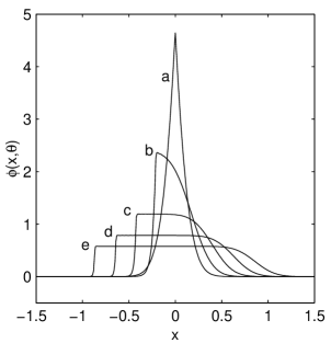
This form is an evident generalization of a track energy introduced in ref.Β [1]. A microstrip sensor integrates on y𝑦y the signal distribution φ​(𝐱,𝐋𝐱)πœ‘π±subscript𝐋𝐱\varphi(\mathbf{x},\mathbf{L_{x}}), and in equationΒ 9 we have Ο‰y=0subscriptπœ”π‘¦0\omega_{y}=0. The surviving Ο‰xsubscriptπœ”π‘₯\omega_{x} variable will be indicated with Ο‰πœ”\omega, and φ​(x)πœ‘π‘₯\varphi(x) the integrated signal distribution. FigureΒ 2 illustrates φ​(x)πœ‘π‘₯\varphi(x) at various incidence angles (Lx=tan⁑(ΞΈ)subscript𝐿π‘₯πœƒL_{x}=\tan(\theta)). The COG of each φ​(x,ΞΈ)πœ‘π‘₯πœƒ\varphi(x,\theta) is in the origin x=0π‘₯0x=0.

Refer to caption
Figure 2: Form of the signal distribution at various incidence angles. The curves aπ‘Ža, b𝑏b, c𝑐c, d𝑑d ed e𝑒e are respectively for ΞΈ=0βˆ˜πœƒsuperscript0\theta=0^{\circ}, ΞΈ=5βˆ˜πœƒsuperscript5\theta=5^{\circ}, ΞΈ=10βˆ˜πœƒsuperscript10\theta=10^{\circ}, ΞΈ=15βˆ˜πœƒsuperscript15\theta=15^{\circ} and ΞΈ=20βˆ˜πœƒsuperscript20\theta=20^{\circ}

3.3 Expressions for the COG and Energy

The asymmetric signal distributions require a slight generalization of the equations in ref.Β [1], where symmetric signals were assumed. The equations of the COG-algorithms with two and three strips will be considered. As in ref.Β [1] we indicate with SΡ​(Ο‰)subscriptSπœ€πœ”\mathrm{S}_{\varepsilon}(\omega) the FT of the sampled convolution of the signal (transformed in a periodic signal with a period T≫τmuch-greater-thanabsent𝜏\gg\tau) with the strip response. The derivative of SΡ​(Ο‰)subscriptSπœ€πœ”\mathrm{S}_{\varepsilon}(\omega) respect to Ο‰πœ”\omega (normalized with SΡ​(0)subscriptSπœ€0\mathrm{S}_{\varepsilon}(0)) is the COG position of the signals collected by the strips. The parameter Ξ΅πœ€\varepsilon is the COG position of the initial signal distribution, and the shift theorem of FT introduces its functional dependence in the equations:

SΡ​(Ο‰)=βˆ‘n=βˆ’βˆž+∞Φnp​P​(2​n​πT)​exp⁑(βˆ’i​2​n​π​ΡT)​H​(Ο‰βˆ’2​n​πT).subscriptSπœ€πœ”superscriptsubscript𝑛superscriptsubscriptΦ𝑛𝑝P2π‘›πœ‹π‘‡π‘–2π‘›πœ‹πœ€π‘‡Hπœ”2π‘›πœ‹π‘‡\mathrm{S}_{\varepsilon}(\omega)=\sum_{n=-\infty}^{+\infty}\Phi_{n}^{p}\ \mathrm{P}(\frac{2n\pi}{T})\exp(\frac{-i2n\pi\varepsilon}{T})\mathrm{H}(\omega-\frac{2n\pi}{T})\,. (10)

In equationΒ 10,   P​(2​n​π/T)P2π‘›πœ‹π‘‡\mathrm{P}(2n\pi/T) is the FT of the strip response function p(x)π‘₯(x), and it will be determined in the following. Ξ¦npsuperscriptsubscriptΦ𝑛𝑝\Phi_{n}^{p} is equationΒ 9 for Ο‰=2​π​n/Tπœ”2πœ‹π‘›π‘‡\omega=2\pi n/T as imposed by periodicity:

Ξ¦np=1T​Φ​(Lx,2​π​nT).superscriptsubscriptΦ𝑛𝑝1𝑇Φsubscript𝐿π‘₯2πœ‹π‘›π‘‡\Phi_{n}^{p}=\frac{1}{T}\Phi(L_{x},\frac{2\pi n}{T})\,. (11)

H​(Ο‰)Hπœ”\mathrm{H}(\omega) is a function of the strip number used in the algorithm. In the case of two strips it is (Ο„πœ\tau is the strip dimension) :

H​(Ο‰)=1+e(βˆ’i​ω​τ)Ξ΅>0formulae-sequenceHπœ”1superscripteπ‘–πœ”πœπœ€0\displaystyle\mathrm{H}(\omega)=1+\mathrm{e}^{(-i\omega\tau)}\qquad\varepsilon>0
H​(Ο‰)=1+e(+i​ω​τ)Ξ΅<0formulae-sequenceHπœ”1superscripteπ‘–πœ”πœπœ€0\displaystyle\mathrm{H}(\omega)=1+\mathrm{e}^{(+i\omega\tau)}\qquad\varepsilon<0

and for three strips:

H​(Ο‰)=1+2​cos⁑(ω​τ)Hπœ”12πœ”πœ\displaystyle\mathrm{H}(\omega)=1+2\cos(\omega\tau)\qquad

Due to the normalization of φ​(x)πœ‘π‘₯\varphi(x) and p(x)π‘₯(x), SΡ​(0)subscriptSπœ€0\mathrm{S}_{\varepsilon}(0) is the signal collection efficiency of the algorithm. The efficiency for the three-strip algorithm is given by:

SΡ​(0)=3​P​(0)T+2β€‹βˆ‘n=1+∞P​(2​n​πT)​[1+2​cos⁑(2​n​π​τT)]​Real​[Ξ¦np​exp⁑(βˆ’i​2​n​π​ΡT)]subscriptSπœ€03P0𝑇2superscriptsubscript𝑛1P2π‘›πœ‹π‘‡delimited-[]122π‘›πœ‹πœπ‘‡Realdelimited-[]superscriptsubscriptΦ𝑛𝑝𝑖2π‘›πœ‹πœ€π‘‡\mathrm{S}_{\varepsilon}(0)=\frac{3\ \mathrm{P}(0)}{T}+2\sum_{n=1}^{+\infty}\ \mathrm{P}(\frac{2n\pi}{T})\big{[}1+2\cos(\frac{2n\pi\tau}{T})\big{]}\mathrm{Real}[\Phi_{n}^{p}\exp(-i\frac{2n\pi\varepsilon}{T})] (12)

and the three-strip COG is:

xg​3=βˆ’4​τSΡ​(0)β€‹βˆ‘n=1+∞P​(2​n​πT)​sin⁑(2​n​π​τT)​Imag​[Ξ¦np​exp⁑(βˆ’i​2​n​π​ΡT)]subscriptπ‘₯𝑔34𝜏subscriptSπœ€0superscriptsubscript𝑛1P2π‘›πœ‹π‘‡2π‘›πœ‹πœπ‘‡Imagdelimited-[]superscriptsubscriptΦ𝑛𝑝𝑖2π‘›πœ‹πœ€π‘‡x_{g3}=\frac{-4\tau}{\mathrm{S}_{\varepsilon}(0)}\sum_{n=1}^{+\infty}\ \mathrm{P}(\frac{2n\pi}{T})\sin(\frac{2n\pi\tau}{T})\,\mathrm{Imag}[\Phi_{n}^{p}\exp(-i\frac{2n\pi\varepsilon}{T})] (13)

If in equationΒ 10 we substitute H​(Ο‰)=exp⁑(βˆ’i​ω​l​τ)π»πœ”π‘–πœ”π‘™πœH(\omega)=\exp(-i\omega l\tau) of a single strip at lβ€‹Ο„π‘™πœl\tau, the expression of SΡ​(Ο‰)subscriptSπœ€πœ”\mathrm{S}_{\varepsilon}(\omega) for Ο‰β†’0β†’πœ”0\omega\rightarrow 0 gives the fraction of the energy collected by the l𝑙l-th strip:

EΞ΅l=βˆ‘n=βˆ’βˆž+∞Φnp​P​(2​π​nT)​exp⁑[βˆ’i​2​π​nT​(Ξ΅βˆ’l​τ)].superscriptsubscriptπΈπœ€π‘™superscriptsubscript𝑛superscriptsubscriptΦ𝑛𝑝𝑃2πœ‹π‘›π‘‡π‘–2πœ‹π‘›π‘‡πœ€π‘™πœE_{\varepsilon}^{l}=\sum_{n=-\infty}^{+\infty}\Phi_{n}^{p}\,P(\frac{2\pi n}{T})\exp\big{[}-i\frac{2\pi n}{T}(\varepsilon-l\tau)\big{]}. (14)

EquationΒ 14 is another way to write the convolution of φ​(xβˆ’Ξ΅)πœ‘π‘₯πœ€\varphi(x-\varepsilon) with p​(x)𝑝π‘₯p(x) for a strip. The periodicity imposed to φ​(x)πœ‘π‘₯\varphi(x) allows to write the convolution as Fourier Series (FS) with all the benefits to use a fast converging discrete sum in place of an integral. So, for the three strip COG xg​3subscriptπ‘₯𝑔3x_{g3}, we can use equationΒ 13 or use xg​3=(EΞ΅1βˆ’EΞ΅βˆ’1)/(EΞ΅1+EΞ΅0+EΞ΅βˆ’1)subscriptπ‘₯𝑔3superscriptsubscriptπΈπœ€1superscriptsubscriptπΈπœ€1superscriptsubscriptπΈπœ€1superscriptsubscriptπΈπœ€0superscriptsubscriptπΈπœ€1x_{g3}=(E_{\varepsilon}^{1}-E_{\varepsilon}^{-1})/(E_{\varepsilon}^{1}+E_{\varepsilon}^{0}+E_{\varepsilon}^{-1}). The last one will be preferred to be consistent with the simulations.

3.4 The Reconstruction of φ​(x)πœ‘π‘₯\varphi(x)

Equation 14 requires further information that we have to extract from the data; a reasonable form of the strip response function p​(x)𝑝π‘₯p(x) (with FT P​(2​n​π/T)P2π‘›πœ‹π‘‡\mathrm{P}(2n\pi/T)) and the best value of α𝛼\alpha of equationΒ 9. These sensor properties are bound together and we must fix their better combination with successive tests. We have some relations to use for this task. The relation, proved in refΒ [1], of d​xg​(Ξ΅)/d​Ρ𝑑subscriptπ‘₯π‘”πœ€π‘‘πœ€d\,x_{g}(\varepsilon)/d\,\varepsilon with φ​(x)πœ‘π‘₯\varphi(x) can be used as a starting point. In that case the response function was an interval function (Π​(x)=1Ξ π‘₯1\Pi(x)=1 for |x|<1/2π‘₯12|x|<1/2 and zero elsewhere). For d​xg​(Ξ΅)/d​Ρ𝑑subscriptπ‘₯π‘”πœ€π‘‘πœ€d\,x_{g}(\varepsilon)/d\,\varepsilon we have (Φ​(Ο‰)Ξ¦πœ”\Phi(\omega) FT of φ​(x)πœ‘π‘₯\varphi(x)) :

d​xgd​Ρ=1+βˆ‘k=1+∞(βˆ’1)k​real​[exp⁑(2​k​π​Ρτ)​Φ​(βˆ’2​k​πτ)]𝑑subscriptπ‘₯π‘”π‘‘πœ€1superscriptsubscriptπ‘˜1superscript1π‘˜realdelimited-[]2π‘˜πœ‹πœ€πœΞ¦2π‘˜πœ‹πœ\frac{dx_{g}}{d\varepsilon}=1+\sum_{k=1}^{+\infty}(-1)^{k}\mathrm{real}\Big{[}\exp\big{(}\frac{2k\pi\varepsilon}{\tau}\big{)}\Phi(-\frac{2k\pi}{\tau})\Big{]}

which for Poisson identityΒ [7] can be reassembled into (with Φ​(0)=1Ξ¦01\Phi(0)=1):

d​xgd​Ρ=βˆ‘k=βˆ’βˆž+∞exp⁑[i​2​k​πτ​(Ο΅βˆ’Ο„2)]​Φ​(βˆ’2​k​πτ)=Ο„β€‹βˆ‘L=βˆ’βˆž+βˆžΟ†β€‹(βˆ’Ξ΅+Ο„2βˆ’L​τ).𝑑subscriptπ‘₯π‘”π‘‘πœ€superscriptsubscriptπ‘˜π‘–2π‘˜πœ‹πœitalic-ϡ𝜏2Ξ¦2π‘˜πœ‹πœπœsuperscriptsubscriptπΏπœ‘πœ€πœ2𝐿𝜏\frac{dx_{g}}{d\varepsilon}=\sum_{k=-\infty}^{+\infty}\exp\big{[}i\frac{2k\pi}{\tau}(\epsilon-\frac{\tau}{2})\big{]}\ \Phi(-\frac{2k\pi}{\tau})=\tau\sum_{L=-\infty}^{+\infty}\varphi(-\varepsilon+\frac{\tau}{2}-L\tau). (15)

If the support of φ​(x)πœ‘π‘₯\varphi(x) is ≀τabsent𝜏\leq\tau , the multiplication of equationΒ 15 by Π​(βˆ’x/Ο„+1/2)Ξ π‘₯𝜏12\Pi(-x/\tau+1/2) reconstructs exactly the function φ​(βˆ’x+Ο„/2)πœ‘π‘₯𝜏2\varphi(-x+\tau/2). It is easy to extract from the reconstruction theoremΒ 15 a relation of peaks in the COG probability distribution and discontinuities in the response function. In regular detector and a φ​(x)πœ‘π‘₯\varphi(x) for ΞΈ=0πœƒ0\theta=0, one has a peak in the COG probability distribution and a discontinuity in p​(x)𝑝π‘₯p(x) at the strip border. In a detector with floating strip the COG probability has three peaks, and we can guess that other discontinuities are present in the response function.

4 The Response Function

4.1 Crosstalk

The set of candidate response function p​(x)𝑝π‘₯p(x) will be selected among the ones defined inΒ [1] as uniform crosstalk, i.e. response function with its influence extending outside the range of a strip and conserving the energy (in the case of an infinite sampling). A sufficient condition for the uniform crosstalk is to have arbitrary functions (even Dirac δ𝛿\delta-function) convoluted with an interval function of size Ο„πœ\tau. In the following we will work with Ο„=1𝜏1\tau=1.

This p​(x)𝑝π‘₯p(x) is suitable to simulate the effect of a floating strip:

p(x)=βˆ«βˆ’βˆž+∞Π(xβˆ’xβ€²){\displaystyle p(x)=\int_{-\infty}^{+\infty}\Pi(x-x^{\prime})\big{\{} a1​[δ​(xβ€²βˆ’1/4)+δ​(xβ€²+1/4)]subscriptπ‘Ž1delimited-[]𝛿superscriptπ‘₯β€²14𝛿superscriptπ‘₯β€²14\displaystyle a_{1}\;[\delta(x^{\prime}-1/4)+\;\delta(x^{\prime}+1/4)] (16)
+a2[Ξ΄(xβ€²βˆ’1/2)+Ξ΄(xβ€²+1/2)]}\displaystyle+a_{2}[\;\delta(x^{\prime}-1/2)+\;\delta(x^{\prime}+1/2)]\big{\}}
Refer to caption
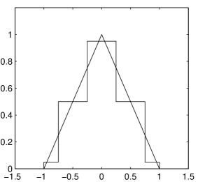
Figure 3: Response function of equationΒ 16 with a1=0.45subscriptπ‘Ž10.45a_{1}=0.45 and a2=0.05subscriptπ‘Ž20.05a_{2}=0.05, a type of uniform crosstalk that reproduces the lateral peaks around xg=Β±1/2subscriptπ‘₯𝑔plus-or-minus12x_{g}=\pm 1/2. The triangular response function (with base 2) is reported for comparison

It is easy to show that the p​(x)𝑝π‘₯p(x) of figureΒ 3 produces the three typical peaks of the Ξ·πœ‚\eta distributionΒ [5] (Ξ·=EL/(EL+ER)πœ‚subscript𝐸𝐿subscript𝐸𝐿subscript𝐸𝑅\eta=E_{L}/(E_{L}+E_{R}) where ELsubscript𝐸𝐿E_{L} and ERsubscript𝐸𝑅E_{R} are the left and right strips of the two largest signal couples) of a floating strip sensor. In fact, figureΒ 3 can be read as the plot of the possible energies collected by the strips in the case of a Dirac δ𝛿\delta signal. The ordinate of each strip center in the array are just the energies collected by an event. Given the strip pitch Ο„=1𝜏1\tau=1, the sample of events is generated by moving the strip array to cover a strip interval. Two possible combination of energy are allowed: equal energies or 0.9 an 0.05. The ratio of one of this pair of energies divided by the sum of the two, gives three δ𝛿\delta-like peaks at the positions 0.054, 0.5, 0.94 and relative intensity (1 2 1). A smearing of the response function with a realistic signal distribution and further fine tuning is able to reproduce the experimental distributions.

The results of an experiment with an infrared laser on a double sided silicon sensorΒ [8] show an energy collection similar to figureΒ 3. In their figure 6 a step-like plot is easily recognized. The due differences must be kept in mind; the laser beam is not a Dirac δ𝛿\delta-function, the strip metallization is opaque to the laser beam.

The response function of equationΒ 16 with a1=0.5subscriptπ‘Ž10.5a_{1}=0.5 and a2=0subscriptπ‘Ž20a_{2}=0 and Φ​(Ο‰)Ξ¦πœ”\Phi(\omega) FT of φ​(x)πœ‘π‘₯\varphi(x) gives for the COG (infinite sampling) the equation:

xg​(Ξ΅)=Ξ΅βˆ’iβ€‹βˆ‘mβ‰ 0,m=βˆ’βˆž+∞(βˆ’1)m4​m​π​Φ​(βˆ’4​π​m)​ei​4​π​m​Ρsubscriptπ‘₯π‘”πœ€πœ€π‘–superscriptsubscriptformulae-sequenceπ‘š0π‘šsuperscript1π‘š4π‘šπœ‹Ξ¦4πœ‹π‘šsuperscripte𝑖4πœ‹π‘šπœ€x_{g}(\varepsilon)=\varepsilon-i\sum_{m\neq 0,m=-\infty}^{+\infty}\frac{(-1)^{m}}{4m\pi}\Phi(-4\pi m)\mathrm{e}^{i4\pi m\varepsilon} (17)

Deriving in Ξ΅πœ€\varepsilon, the Poisson identity gives:

d​xgd​Ρ=12β€‹βˆ‘l=βˆ’βˆž+βˆžΟ†β€‹(βˆ’Ξ΅+14βˆ’l2)dsubscriptπ‘₯𝑔dπœ€12superscriptsubscriptπ‘™πœ‘πœ€14𝑙2\frac{\mathrm{d}x_{g}}{\mathrm{d}\varepsilon}=\frac{1}{2}\sum_{l=-\infty}^{+\infty}\varphi(-\varepsilon+\frac{1}{4}-\frac{l}{2}) (18)

The equationΒ 18 is a sum of infinite copies of φ​(x)πœ‘π‘₯\varphi(x) centered at 1/4 and 3/4 of each strip. It will be used as a guide to select a response function p(x)π‘₯(x) for the simulations.

4.2 Probability Distribution

As we discussed in ref.Β [1], given an identical signal distribution for each event, the probability Γ​(xg)Ξ“subscriptπ‘₯𝑔\Gamma(x_{g}) to have xgsubscriptπ‘₯𝑔x_{g} ( for each algorithm) is the product of the probability P(Ξ΅)πœ€(\varepsilon) to have Ξ΅πœ€\varepsilon and |d​Ρ​(xg)/d​xg|dπœ€subscriptπ‘₯𝑔dsubscriptπ‘₯𝑔|\mathrm{d}\varepsilon(x_{g})/\mathrm{d}x_{g}|:

Γ​(xg)=P​(Ξ΅)​|d​Ρ​(xg)d​xg|Ξ“subscriptπ‘₯𝑔Pπœ€π‘‘πœ€subscriptπ‘₯𝑔𝑑subscriptπ‘₯𝑔\Gamma(x_{g})=\mathrm{P}(\varepsilon)\Big{|}\frac{d\varepsilon(x_{g})}{dx_{g}}\Big{|} (19)

This equation could be handled as a differential equation, if we prove that the unknown function has always the same sign. We showed inΒ [1] that d​Ρ/d​xgπ‘‘πœ€π‘‘subscriptπ‘₯𝑔d\varepsilon/dx_{g} is non negative for a large set of signal distribution and algorithms with different number of strips. For an infinite sampling, equationsΒ 15 andΒ 18 show immediately that d​xg/d​Ρdsubscriptπ‘₯𝑔dπœ€\mathrm{d}x_{g}/\mathrm{d}\varepsilon is always non negative if φ​(Ξ΅)πœ‘πœ€\varphi(\varepsilon) is non negative.

In real events, the conditions giving equationΒ 19 are always violated. The noise is present, the charge deposition fluctuates, different strips are hit in different events, and we never have a single Ρ​(xg)πœ€subscriptπ‘₯𝑔\varepsilon(x_{g}). The experimental probability distribution is an average over different type of signals produced by the particles and of responses of different strips of the detector. Being the probability an average over fluctuations, also the reconstruction will be an average, and it will be effective if the fluctuations and the noise is not too high. With these limitations in mind and for a constant P(Ξ΅)πœ€(\varepsilon), the equationΒ (19) is easy to solve given an initial condition:

Ρ​(xg)=Ο„β€‹βˆ«xg0xgΓ​(y)​𝑑y+Ρ​(xg0).πœ€subscriptπ‘₯π‘”πœsuperscriptsubscriptsuperscriptsubscriptπ‘₯𝑔0subscriptπ‘₯𝑔Γ𝑦differential-dπ‘¦πœ€superscriptsubscriptπ‘₯𝑔0\varepsilon(x_{g})=\tau\int_{x_{g}^{0}}^{x_{g}}\Gamma(y)dy+\varepsilon(x_{g}^{0}). (20)

The selection of the initial condition Ρ​(xg0)πœ€superscriptsubscriptπ‘₯𝑔0\varepsilon(x_{g}^{0}) is a critical point, we will see in the following, for ΞΈβ‰ 0πœƒ0\theta\neq 0, the amplitude of the systematic error given by the error on Ρ​(xg0)πœ€superscriptsubscriptπ‘₯𝑔0\varepsilon(x_{g}^{0}) .

To simplify, the symmetry of the strip response p​(x)𝑝π‘₯p(x) will be assumed. So, for symmetric φ​(x)πœ‘π‘₯\varphi(x), two points have the property xg​(Ξ΅)=Ξ΅subscriptπ‘₯π‘”πœ€πœ€x_{g}(\varepsilon)=\varepsilon: xg​(Β±1/2)=Β±1/2subscriptπ‘₯𝑔plus-or-minus12plus-or-minus12x_{g}(\pm 1/2)=\pm 1/2 and xg​(0)=0subscriptπ‘₯𝑔00x_{g}(0)=0. In this case the initial condition is exactly defined.

4.3 The Data

To fine tuning our simulation, we need a comparison with experimental data. The data used are obtained from a test beam of a tracker prototype for the PAMELAΒ [9] experiment.

The beam particles are Ο€+superscriptπœ‹\pi^{+} and the incidence angle is orthogonal to the plane of the sensors. Each sensor is 300 ΞΌπœ‡\mum thick silicon wafer where the junction side and the ohmic side are arranged to position measurements. In the junction side p+superscript𝑝p^{+} strips are implanted and one of two connected to the read out electronics (pitch 50ΞΌπœ‡\mum). The ohmic side has n+superscript𝑛n^{+} strips orthogonal to the strips of the junction side and each n+superscript𝑛n^{+} strips connected to the read out electronics (pitch 67 ΞΌπœ‡\mum). No magnetic field is present.

The sign of the read-out signals is arranged to be independent from the collected charge. The events are selected in a standard way and, after pedestal and common noise subtraction, they are assembled with the data of the maximum-signal strip at the center of an eleven component vector. The other vector components contain the data of the neighboring strips. The pedestal and common noise subtraction attenuates almost completely the ADC quantization.

Low signal values of any sign, contained in the data, are used in the algorithms. No attention is given to the cluster size. We select the events to have the sum of the collected signal in the maximum strip and in its two adjacent greater than 40 ADC counts and lower than 350 ADC counts. In this range of ADC counts the Landau peak is fully contained. We cut the high energy tail where it is probable to have δ𝛿\delta-rays or other reactions, and the low energy tail for its low signal to noise ratio.

The far strip signals are use to estimate the noise and the crosstalk.

The COG algorithms have the origin of their reference system in the center of the strip with the maximum signal. (In section 6 we will abandon this convention and the true position will be considered)

We indicate with xg​nsubscriptπ‘₯𝑔𝑛x_{gn} the COG calculated with n𝑛n strips. The two strip algorithm xg​2subscriptπ‘₯𝑔2x_{g2} has the best signal to noise ratio, but, due to the crosstalk has an appreciable discontinuity in the origin even with ΞΈ=0πœƒ0\theta=0 and regular strips. The noise strongly attenuates the discontinuity, but a drop around xg​2β‰ˆ0subscriptπ‘₯𝑔20x_{g2}\approx 0 is evident in the probability distribution.

The xg​3subscriptπ‘₯𝑔3x_{g3} algorithm tends to have two region of low probability at the strip borders.

The infinite sampling is excluded for the noise, thus we can expect some deviation in the φ​(Ξ΅)πœ‘πœ€\varphi(\varepsilon) reconstructed with Ξ΅πœ€\varepsilon extracted from xg​2subscriptπ‘₯𝑔2x_{g2} and xg​3subscriptπ‘₯𝑔3x_{g3}. These deviations are well localized and we expect that xg​2subscriptπ‘₯𝑔2x_{g2} and xg​3subscriptπ‘₯𝑔3x_{g3} are interesting reconstruction tools outside the regions of strong deviations.

4.4 Position Reconstruction

In the xg​2subscriptπ‘₯𝑔2x_{g2} algorithm, we use maximum-signal strip and the maximum (of any sign) between the two lateral. In the xg​3subscriptπ‘₯𝑔3x_{g3} we use the maximum-signal strip and the two lateral.

We assume that the probability P(Ξ΅)πœ€(\varepsilon) is constant on a strip length after the subtraction of the maximum integer contained in Ξ΅πœ€\varepsilon, and the noise does not destroy the validity of equationΒ 20. The histograms of Γ​(xg​2)Ξ“subscriptπ‘₯𝑔2\Gamma(x_{g2}) and Γ​(xg​3)Ξ“subscriptπ‘₯𝑔3\Gamma(x_{g3}) are inserted in equationΒ 20, and Ξ΅2​(xg​2)subscriptπœ€2subscriptπ‘₯𝑔2\varepsilon_{2}(x_{g2}) and Ξ΅3​(xg​3)subscriptπœ€3subscriptπ‘₯𝑔3\varepsilon_{3}(x_{g3}) are obtained with a numerical integration. The initial condition Ξ΅2,3​(βˆ’1/2)=βˆ’1/2subscriptπœ€231212\varepsilon_{2,3}(-1/2)=-1/2 is used. Due to the noise Ξ΅2,3​(xg​2,3)subscriptπœ€23subscriptπ‘₯𝑔23\varepsilon_{2,3}(x_{g2,3}) are an estimate of the most probable Ξ΅πœ€\varepsilon given xg​2,3subscriptπ‘₯𝑔23x_{g2,3}. Where Ξ΅2,3subscriptπœ€23\varepsilon_{2,3} or xg​2,3subscriptπ‘₯𝑔23x_{g2,3} indicate simultaneously Ξ΅2subscriptπœ€2\varepsilon_{2} and Ξ΅3subscriptπœ€3\varepsilon_{3} or xg​2subscriptπ‘₯𝑔2x_{g2} and xg​3subscriptπ‘₯𝑔3x_{g3}.

The numerical forms of Ξ΅2,3​(xg​2,3)subscriptπœ€23subscriptπ‘₯𝑔23\varepsilon_{2,3}(x_{g2,3}) are not practical for the successive uses, it is fundamental to have analytical expressions. The natural way to construct analytical expressions is to consider the periodicity of Ρ​(xg)πœ€subscriptπ‘₯𝑔\varepsilon(x_{g}) in presence of a true uniform illumination. This is not our case, but we have to near this condition. Our set of data are scattered on a large set of strips, and it is improbable to have the same strip few times. In the algorithm, we collect together all the signal on a single strip to generate a fictitious uniform illumination on that strip, all the other strips have no illumination. But, due to the uniformity of the strip properties, we can consider all the strips with an identical incident illumination and an identical probability Γ​(xg)Ξ“subscriptπ‘₯𝑔\Gamma(x_{g}), this virtual total probability becomes periodical:

Ξ“p​(xg)=βˆ‘j=βˆ’βˆžβˆžΞ“β€‹(xg+j).superscriptΓ𝑝subscriptπ‘₯𝑔superscriptsubscript𝑗Γsubscriptπ‘₯𝑔𝑗\Gamma^{p}(x_{g})=\sum_{j=-\infty}^{\infty}\Gamma(x_{g}+j)\,.

With Ξ“p​(xg)superscriptΓ𝑝subscriptπ‘₯𝑔\Gamma^{p}(x_{g}), the Fourier series (FS) is the natural way to fit the function Ξ΅nβˆ’xg​nsubscriptπœ€π‘›subscriptπ‘₯𝑔𝑛\varepsilon_{n}-x_{gn} that is itself periodic:

Ξ΅n​(xg​n)βˆ’xg​n=βˆ‘k=βˆ’βˆž+∞αk​ei​2​π​k​xg​nsubscriptπœ€π‘›subscriptπ‘₯𝑔𝑛subscriptπ‘₯𝑔𝑛superscriptsubscriptπ‘˜subscriptπ›Όπ‘˜superscripte𝑖2πœ‹π‘˜subscriptπ‘₯𝑔𝑛\displaystyle\varepsilon_{n}(x_{gn})-x_{gn}=\sum_{k=-\infty}^{+\infty}\alpha_{k}\mathrm{e}^{i2\pi k\,x_{gn}} (21)
xg​n​(Ξ΅n)βˆ’Ξ΅n=βˆ‘k=βˆ’βˆž+∞βk​ei​2​π​k​Ρnsubscriptπ‘₯𝑔𝑛subscriptπœ€π‘›subscriptπœ€π‘›superscriptsubscriptπ‘˜subscriptπ›½π‘˜superscripte𝑖2πœ‹π‘˜subscriptπœ€π‘›\displaystyle x_{gn}(\varepsilon_{n})-\varepsilon_{n}=\sum_{k=-\infty}^{+\infty}\beta_{k}\mathrm{e}^{i2\pi k\varepsilon_{n}}

The periodicity of Ξ“p​(xg​n)superscriptΓ𝑝subscriptπ‘₯𝑔𝑛\Gamma^{p}(x_{gn}) is a method to handle the events with |xg​n|>1/2subscriptπ‘₯𝑔𝑛12|x_{gn}|>1/2. In the xg​2subscriptπ‘₯𝑔2x_{g2}-algorithm, it is very improbable to have |xg​2|>1/2subscriptπ‘₯𝑔212|x_{g2}|>1/2. The less energetic strip must have a large negative value with its modulus greater than 2/3 the energy of the other strip, and this never happens in our data. In the xg​3subscriptπ‘₯𝑔3x_{g3} algorithm, events with |xg​3|>1/2subscriptπ‘₯𝑔312|x_{g3}|>1/2 are possible, and in the xg​4subscriptπ‘₯𝑔4x_{g4} algorithm an important fraction of events has |xg​4|>1/2subscriptπ‘₯𝑔412|x_{g4}|>1/2.

Given our interest in Ξ΅n​(xg​n)subscriptπœ€π‘›subscriptπ‘₯𝑔𝑛\varepsilon_{n}(x_{gn}), we use the first of the equationsΒ LABEL:eq:106 with a reduced number of terms (Ξ±k=0subscriptπ›Όπ‘˜0\alpha_{k}=0 for |k|β‰₯15π‘˜15|k|\geq 15) to filter the high frequencies of the numerical integration on a small bin-size histogram. The Ξ±ksubscriptπ›Όπ‘˜\alpha_{k} are obtained with another numerical integration with the standard form of the FS coefficients.

Dropping the number of strips in the notation, the derivative d​xg​(Ξ΅)/d​Ρdsubscriptπ‘₯π‘”πœ€dπœ€\mathrm{d}x_{g}(\varepsilon)/\mathrm{d}\varepsilon is given by the identity:

d​xg​(Ξ΅)d​Ρ=1d​Ρ​(xg)d​xg=[1+βˆ‘k=βˆ’βˆž+∞(i​2​π​k)​αk​ei​2​π​k​xg]βˆ’1.dsubscriptπ‘₯π‘”πœ€dπœ€1dπœ€subscriptπ‘₯𝑔dsubscriptπ‘₯𝑔superscriptdelimited-[]1superscriptsubscriptπ‘˜π‘–2πœ‹π‘˜subscriptπ›Όπ‘˜superscripte𝑖2πœ‹π‘˜subscriptπ‘₯𝑔1\frac{\mathrm{d}x_{g}(\varepsilon)}{\mathrm{d}\varepsilon}=\frac{1}{\frac{\mathrm{d}\varepsilon(x_{g})}{\mathrm{d}x_{g}}}=[1+\sum_{k=-\infty}^{+\infty}(i2\pi k)\alpha_{k}\mathrm{e}^{i2\pi kx_{g}}]^{-1}. (22)

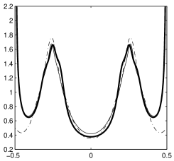
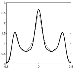
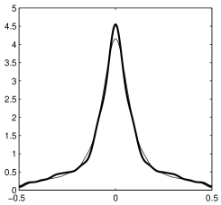
and the plot of the reconstructed φ​(Ξ΅)πœ‘πœ€\varphi(\varepsilon) is generated with Ρ​(xg)πœ€subscriptπ‘₯𝑔\varepsilon(x_{g}) on the xπ‘₯x-axis, and the xgsubscriptπ‘₯𝑔x_{g}-function of equationΒ 22 on the y𝑦y-axis. This method is very effective, as we can see in figureΒ 4. Here the xg​3subscriptπ‘₯𝑔3x_{g3} from data and from the simulations are elaborated in the same way. From equationΒ 18 we expect two copies of φ​(Ξ΅3)πœ‘subscriptπœ€3\varphi(\varepsilon_{3}) centered at Β±0.25plus-or-minus0.25\pm 0.25. The similarity of the two reconstructed φ​(Ξ΅3)πœ‘subscriptπœ€3\varphi(\varepsilon_{3}) is noticeable and they are near to the noiseless d​xg​3​(Ξ΅)/d​Ρdsubscriptπ‘₯𝑔3πœ€dπœ€\mathrm{d}x_{g3}(\varepsilon)/\mathrm{d}\varepsilon (obtained deriving the equationΒ 13). The parameter Ξ±=0.0324𝛼0.0324\alpha=0.0324 is used in the simulations. The details of the simulations will be given in the coming section, here we test the response function and the diffusion parameter α𝛼\alpha.

The two lateral increases are typical of the xg​3subscriptπ‘₯𝑔3x_{g3}-algorithm. In the noiseless case, two discontinuities are present in xg​3​(Ξ΅3)subscriptπ‘₯𝑔3subscriptπœ€3x_{g3}(\varepsilon_{3}) at Ξ΅3=Β±1/2subscriptπœ€3plus-or-minus12\varepsilon_{3}=\pm 1/2. The noise smooths the discontinuities in regions of fast variation that give a substantial increases to the derivative. The noiseless xg​3​(Ξ΅)subscriptπ‘₯𝑔3πœ€x_{g3}(\varepsilon) and its derivative (given by the equationΒ 13) are defined in the interior of a single strip and the two Dirac δ𝛿\delta are outside the definition domain.

Refer to caption
Refer to caption
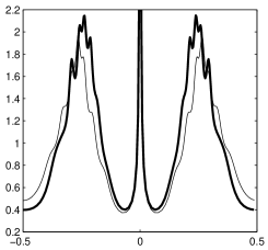
Figure 4: To the left φ​(Ξ΅)πœ‘πœ€\varphi(\varepsilon) obtained by the xg​3subscriptπ‘₯𝑔3x_{g3} algorithm applied to the data (thick line), given by the simulations (thin line), and deriving equationΒ 13 (dash-dot line). To the right the algorithm is xg​2subscriptπ‘₯𝑔2x_{g2}, the thick line is given by the data, the thin line by the simulations.

To see the effect of limited sampling, in the left side of figureΒ 4 the equationΒ 22 is applied to Ξ΅2​(xg​2)subscriptπœ€2subscriptπ‘₯𝑔2\varepsilon_{2}(x_{g2}) given by the data and by the simulations. Even here the two reconstructions are similar, and similar is the number of oscillations, these are given by the lower number of events respect to the regions with Ξ΅β‰ˆ0πœ€0\varepsilon\approx 0 and Ξ΅β‰ˆΒ±1/2πœ€plus-or-minus12\varepsilon\approx\pm 1/2. The large increase for Ξ΅=0πœ€0\varepsilon=0 is typical of xg​2subscriptπ‘₯𝑔2x_{g2} that has there a discontinuity in the absence of noise.
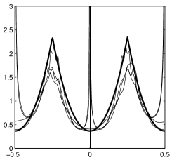
The result of equationΒ 18 is reported in figureΒ 5 with all the reconstructions of figureΒ 4.

Refer to caption
Refer to caption
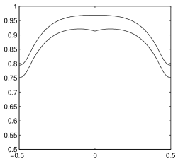
Figure 5: The thick line is φ​(Ξ΅)πœ‘πœ€\varphi(\varepsilon) as given by equationΒ 18, the thin lines are the other reconstructions of figuresΒ 4. To the right, the efficiency of xg3subscriptπ‘₯subscript𝑔3x_{g_{3}} (higher curve) and of xg2subscriptπ‘₯subscript𝑔2x_{g_{2}} (lower curve). The signal loss is visible as the drop around Β±0.5plus-or-minus0.5\pm 0.5.

5 Simulations

5.1 Event Generation

To generate the events, we use the following procedure. A set of random points {Ξ΅i}subscriptπœ€π‘–\{\varepsilon_{i}\} is generated with an uniform distribution on 3 strips. The points Ξ΅isubscriptπœ€π‘–\varepsilon_{i} are used to calculate the fraction of energy EΞ΅ilsuperscriptsubscript𝐸subscriptπœ€π‘–π‘™E_{\varepsilon_{i}}^{l} (equationΒ 14) for five strips {l}𝑙\{l\} centered around the strip containing Ξ΅isubscriptπœ€π‘–\varepsilon_{i}. For each event, a random number is extracted with the distribution of the total experimental charge (in ADC counts) collected by three strips (the one with the maximum signal and the two adjacent). All the EΞ΅ilsuperscriptsubscript𝐸subscriptπœ€π‘–π‘™E_{\varepsilon_{i}}^{l} of the event i𝑖i are scaled with this random factor. The noise is added to each strip with a gaussian distribution modelled from the data.

5.2 Losses

Further details must be defined to fine tuning our simulations to the data. From the beginning, we suppose that the signal shape is the same at least on average. The noise and the fluctuations of the primary ionization modify the pattern of the collected energy for each events, but the xgsubscriptπ‘₯𝑔x_{g}-histograms must not change. On the contrary, the xgsubscriptπ‘₯𝑔x_{g}-histograms for events with energy less than the Landau maximum (175 ADC counts for our data) have a larger probability for |xg|β‰ˆ1/2subscriptπ‘₯𝑔12|x_{g}|\approx 1/2 than the events with higher energies. An easy explanation of these differences can be a signal loss in the detector interior around the floating strip.

We can simulate this loss with an efficiency reduction around the strip borders. Cutting two grooves around x=Β±1/2π‘₯plus-or-minus12x=\pm 1/2 on p​(x)𝑝π‘₯p(x), one obtains the efficiency plots of figureΒ 5. The efficiency drop around x=Β±0.5π‘₯plus-or-minus0.5x=\pm 0.5 is exclusively given by the loss. This type of loss is qualitatively similar to that measured in refΒ [10]; in our case it is guessed by the xg​2,3subscriptπ‘₯𝑔23x_{g2,3}-probability plots for events with different total energy.

5.3 Long Range Crosstalk

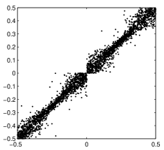
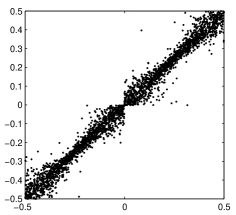
In sectionΒ 4.1 we discussed the main crosstalk produced by the floating strip. But, in the strips adjacent to that used in xg​3subscriptπ‘₯𝑔3x_{g3}, we see an average shift of the collected signals toward the maximum signal strip. This means that a long range crosstalk is present in the data. To produce detailed simulations, other terms must be added to p​(x)𝑝π‘₯p(x) with tails longer than that of figureΒ 3. In figureΒ 6, the effect of the crosstalk (and the quality of the simulations) is clearly seen. Here Ξ΅3​(xg​3​(j))subscriptπœ€3subscriptπ‘₯𝑔3𝑗\varepsilon_{3}(x_{g3}(j)) vs Ξ΅2​(xg​2​(j))subscriptπœ€2subscriptπ‘₯𝑔2𝑗\varepsilon_{2}(x_{g2}(j)) for data events and for simulated events can be compared, it is evident a strict similarity of the distribution patterns. The total elimination of all the crosstalk drastically modifies the scatter plot as can be see in the plots of figureΒ 9.

Refer to caption
Refer to caption
Figure 6: Samples of {Ξ΅3​(xg​3​(j)),Ξ΅2​(xg​2​(j))}subscriptπœ€3subscriptπ‘₯𝑔3𝑗subscriptπœ€2subscriptπ‘₯𝑔2𝑗\{\varepsilon_{3}(x_{g3}(j)),\varepsilon_{2}(x_{g2}(j))\}. To the left the data. To the right the simulations. Identical forbidden regions are present in the two scatter plots.

5.4 Data and Simulations

The consistency of the simulations with the data can be appreciated in figureΒ 7. Here the probability distributions of Ξ“p​xg​3superscriptΓ𝑝subscriptπ‘₯𝑔3\Gamma^{p}x_{g3} are compared. The two curves are obtained from equationΒ LABEL:eq:106, but this time we plot d​Ρ​(xg​3)/d​xg​3dπœ€subscriptπ‘₯𝑔3dsubscriptπ‘₯𝑔3\mathrm{d}\varepsilon(x_{g3})/\mathrm{d}x_{g3} versus xg​3subscriptπ‘₯𝑔3x_{g3}. This is apparently a trivial operation, first Ξ“p​(xg​3)superscriptΓ𝑝subscriptπ‘₯𝑔3\Gamma^{p}(x_{g3}) is integrated an after it is derived to return to Ξ“p​(xg​3)superscriptΓ𝑝subscriptπ‘₯𝑔3\Gamma^{p}(x_{g3}). In reality this procedure applies a consistent low pass filter to Ξ“p​(xg​3)superscriptΓ𝑝subscriptπ‘₯𝑔3\Gamma^{p}(x_{g3}).

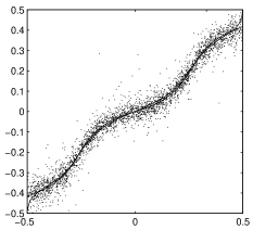
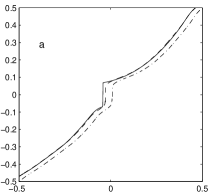
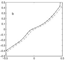
FigureΒ 8 reports a sample of simulated xg​2subscriptπ‘₯𝑔2x_{g2} and xg​3subscriptπ‘₯𝑔3x_{g3} values. The two overlapping lines are xg​2​(Ξ΅2)subscriptπ‘₯𝑔2subscriptπœ€2x_{g2}(\varepsilon_{2}) obtained from simulated events with noise and the noiseless xg​2​(Ξ΅)subscriptπ‘₯𝑔2πœ€x_{g2}(\varepsilon). If we exclude a smoothing in the rapid variation regions (around xg​2=0subscriptπ‘₯𝑔20x_{g2}=0), the overlap is almost complete. The noise works as a low pass filter. Similar overlap is observed even for the noisy xg​3​(Ξ΅3)subscriptπ‘₯𝑔3subscriptπœ€3x_{g3}(\varepsilon_{3})) with the plot of noiseless xg​3​(Ξ΅)subscriptπ‘₯𝑔3πœ€x_{g3}(\varepsilon)). In spite of these overlaps, the error Ξ΅2,3​(xg​2,3)βˆ’Ξ΅subscriptπœ€23subscriptπ‘₯𝑔23πœ€\varepsilon_{2,3}(x_{g2,3})-\varepsilon remains appreciable. In fact, the reconstruction algorithm Ξ΅2,3​(xg​2,3)subscriptπœ€23subscriptπ‘₯𝑔23\varepsilon_{2,3}(x_{g2,3}) explores the scatter-plot of figureΒ 8 along the horizontal line going through xg​2,3subscriptπ‘₯𝑔23x_{g2,3}. The noise shifts xg​2,3subscriptπ‘₯𝑔23x_{g2,3} along a vertical line passing through the noiseless xg​2,3​(Ξ΅)subscriptπ‘₯𝑔23πœ€x_{g2,3}(\varepsilon). If the shift is large and/or the slope of xg​2,3​(Ξ΅2,3)subscriptπ‘₯𝑔23subscriptπœ€23x_{g2,3}(\varepsilon_{2,3}) is small the error is large.

The easy agreement of the simulations with the data (and the small error of the φ​(x)πœ‘π‘₯\varphi(x)-reconstructions) allows to state that the key point of the simulations for the detector with floating strips is a response function p​(x)𝑝π‘₯p(x) with the form of figureΒ 3. This p​(x)𝑝π‘₯p(x) gives even an explanation of the better quality of the reconstruction (and of its error almost independent from ΞΈπœƒ\theta, as it will be seen in the following). In fact, for signal distributions of the size used, its effect is similar to a triangular p​(x)𝑝π‘₯p(x) with base 2​τ2𝜏2\tau. As proved in ref.Β [1], the triangular function with base 2​τ2𝜏2\tau is one of the response function that are free from the COG discretizzation error for any signal distribution (ideal detector). The noise and the information loss, due to a restricted number of strips used in the algorithm, are the most significant limiting factors in the reconstruction, and a true triangular p​(x)𝑝π‘₯p(x) gives modest improvements.

Refer to caption
Figure 7: Probability distribution Ξ“p​(xg​3)superscriptΓ𝑝subscriptπ‘₯𝑔3\Gamma^{p}(x_{g3}) of the simulation (thin line) and of the data (thick line).
Refer to caption
Refer to caption
Figure 8: To the left, the xg​2subscriptπ‘₯𝑔2x_{g2}-positions in function of the corresponding Ξ΅πœ€\varepsilon for the simulated events. The two overlapping curves are: xg​2​(Ξ΅2)subscriptπ‘₯𝑔2subscriptπœ€2x_{g2}(\varepsilon_{2}) and the noiseless xg​2​(Ξ΅)subscriptπ‘₯𝑔2πœ€x_{g2}(\varepsilon). To the right, xg​3subscriptπ‘₯𝑔3x_{g3} and Ξ΅πœ€\varepsilon for the simulated events. The two overlapping curves are xg​3​(Ξ΅3)subscriptπ‘₯𝑔3subscriptπœ€3x_{g3}(\varepsilon_{3}) and the noiseless xg​3​(Ξ΅)subscriptπ‘₯𝑔3πœ€x_{g3}(\varepsilon).

6 Normal-strip side

6.1 The Response Function

The ohmic-side of the sensor has no floating strips, we will call normal strip side the ohmic-side, and normal strips its strips.

The lack of a capacitive coupling in this side produces a large reconstruction error. For ΞΈ=0βˆ˜πœƒsuperscript0\theta=0^{\circ}, an important fraction of the signal tends to concentrate on a single strip giving an high probability to have xg​2,3β‰ˆ0subscriptπ‘₯𝑔230x_{g2,3}\approx 0. A small interstrip capacity is present, but its crosstalk effect remains modest. At any rate, to produce a good simulation, we have to account for this crosstalk with the following empirical response function p​(x)𝑝π‘₯p(x):

p​(x)=𝑝π‘₯absent\displaystyle p(x)= βˆ«βˆ’βˆž+∞dxβ€²Ξ (xβˆ’xβ€²){0.91Ξ΄(xβ€²)+0.063[Ξ΄(xβ€²βˆ’Ο„/2)+Ξ΄(xβ€²+Ο„/2)]\displaystyle\int_{-\infty}^{+\infty}\mathrm{d}x^{\prime}\,\Pi(x-x^{\prime})\Big{\{}0.91\delta(x^{\prime})+0.063[\delta(x^{\prime}-\tau/2)+\delta(x^{\prime}+\tau/2)] (23)
+0.027[Ξ΄(xβ€²βˆ’3Ο„/2)+Ξ΄(xβ€²+3Ο„/2)]}\displaystyle+0.027[\delta(x^{\prime}-3\tau/2)+\delta(x^{\prime}+3\tau/2)]\Big{\}}

The main part of p​(x)𝑝π‘₯p(x) is given by 0.91​Π​(x)0.91Ξ π‘₯0.91\,\Pi(x) (i.e., an interval function), and the small terms are selected to produce an uniform crosstalk. p​(x)𝑝π‘₯p(x) is fine tuned to produce a good agreement of the histograms (and cross-correlations) obtained from the simulation with the corresponding obtained from the data.

Refer to caption
Figure 9: Samples of {Ξ΅3​(xg​3​(j)),Ξ΅2​(xg​2​(j))}subscriptπœ€3subscriptπ‘₯𝑔3𝑗subscriptπœ€2subscriptπ‘₯𝑔2𝑗\{\varepsilon_{3}(x_{g3}(j)),\varepsilon_{2}(x_{g2}(j))\}. Figure a) for the data, b) the simulations with crosstalk, and c) the simulations without the crosstalk .

In figureΒ 9, we show the correlation of Ξ΅3​(xg​3​(j))subscriptπœ€3subscriptπ‘₯𝑔3𝑗\varepsilon_{3}(x_{g3}(j)) vs. Ξ΅2​(xg​2​(j))subscriptπœ€2subscriptπ‘₯𝑔2𝑗\varepsilon_{2}(x_{g2}(j)) in the data, in the simulation with the crosstalk of equationΒ 23, and without crosstalk (p​(x)=Π​(x)𝑝π‘₯Ξ π‘₯p(x)=\Pi(x)). As it is clearly seen, the absence of crosstalk produces a plot drastically different from the data. The crosstalk of equationΒ 23 gives correlations with exclusion regions very similar to the experimental one. This test looks more sensitive than the histograms, here even the noise model can be compared.

6.2 Simulations

The simulated events are generated as in the case of the floating strip, with some evident modifications. The parameter α𝛼\alpha is taken to be 0.02890.02890.0289 (partially scaled to keep into account the difference of Ο„=67β€‹ΞΌπœ67πœ‡\tau=67\mum), and p​(x)𝑝π‘₯p(x) is given by equationΒ 23.

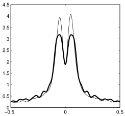
A set of random Ξ΅isubscriptπœ€π‘–\varepsilon_{i} values is generated with an uniform distribution over three strips. The Ξ΅isubscriptπœ€π‘–\varepsilon_{i}-values are the COG of initial ionization distributions. The fraction of the charge collected by each strip is calculated with equationΒ 14, and the simulated collected charge is obtained multiplying by a random factor with a distribution similar to that in the data. A fluctuation with a Poisson distribution is added to the charge collected in each strip. The additive noise is gaussian with zero mean and standard deviation similar to the noise distribution of the distant strips in the data. A comparison of the probability distributions for xg​2subscriptπ‘₯𝑔2x_{g2} and xg​3subscriptπ‘₯𝑔3x_{g3} is reported in figureΒ 10. The plots are produced as explained in sectionΒ 5.4 for the floating strip side. Even in this case the agreement is excellent.
Refer to caption
Refer to caption
Figure 10: To the left, probability distribution for xg​2subscriptπ‘₯𝑔2x_{g2} from the simulations (thin line), and from the data (thick line). To the right, the probability distribution for xg​3subscriptπ‘₯𝑔3x_{g3}; simulations (thin line), data (thick line).

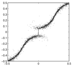
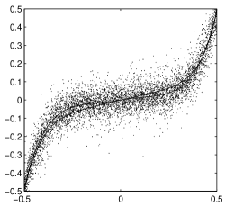
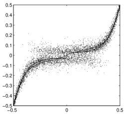
FigureΒ 11 is the equivalent of figureΒ 8 for the normal strip side. Here the simulated events are scattered far from the curves xg​2,3​(Ξ΅2,3)subscriptπ‘₯𝑔23subscriptπœ€23x_{g2,3}(\varepsilon_{2,3}) or the noiseless xg​2,3​(Ξ΅)subscriptπ‘₯𝑔23πœ€x_{g2,3}(\varepsilon), and the position reconstruction with Ξ΅2,3​(xg​2,3)subscriptπœ€23subscriptπ‘₯𝑔23\varepsilon_{2,3}(x_{g2,3}) has a larger error compared to the floating strip side. The overlaps of xg​2,3​(Ξ΅2,3)subscriptπ‘₯𝑔23subscriptπœ€23x_{g2,3}(\varepsilon_{2,3}) with the noiseless xg​2,3​(Ξ΅)subscriptπ‘₯𝑔23πœ€x_{g2,3}(\varepsilon) are smaller than these for the floating strips.
Refer to caption
Refer to caption
Figure 11: To the left, a sample of {Ρ​(j),xg​2​(j)}πœ€π‘—subscriptπ‘₯𝑔2𝑗\{\varepsilon(j),x_{g2}(j)\}, the two curves are: the discontinuous one is the noiseless xg​2​(Ξ΅)subscriptπ‘₯𝑔2πœ€x_{g2}(\varepsilon), the other is xg​2​(Ξ΅2)subscriptπ‘₯𝑔2subscriptπœ€2x_{g2}(\varepsilon_{2}) with Ξ΅2subscriptπœ€2\varepsilon_{2} given by equationΒ 20. To the right, a sample of {Ρ​(j),xg​3​(j)}πœ€π‘—subscriptπ‘₯𝑔3𝑗\{\varepsilon(j),x_{g3}(j)\}. The two curves are the noiseless xg​3​(Ξ΅)subscriptπ‘₯𝑔3πœ€x_{g3}(\varepsilon) and xg​3​(Ξ΅3)subscriptπ‘₯𝑔3subscriptπœ€3x_{g3}(\varepsilon_{3})

7 Directions with ΞΈβ‰ 0πœƒ0\theta\neq 0

7.1 Simulations

The angle ΞΈπœƒ\theta is defined in figureΒ 1, and Lxsubscript𝐿π‘₯L_{x} is given by Lx=L0​tan⁑(ΞΈ)subscript𝐿π‘₯subscript𝐿0πœƒL_{x}=L_{0}\tan(\theta). With Lxβ‰ 0subscript𝐿π‘₯0L_{x}\neq 0, the different diffusion times of the top and the bottom of the track are shifted, and φ​(x)πœ‘π‘₯\varphi(x) becomes asymmetric. FigureΒ 2 shows these asymmetries.

For ΞΈβ‰ 0πœƒ0\theta\neq 0 we have no data consistent with these used for ΞΈ=0πœƒ0\theta=0, and we cannot test the simulations. But, given the agreement reached for ΞΈ=0πœƒ0\theta=0, it is reasonable to proceed with our simulations at least in the range 0βˆ˜β‰€ΞΈβ‰€20∘superscript0πœƒsuperscript200^{\circ}\leq\theta\leq 20^{\circ}. At any rate, we will prove with analytical development our critical results delineated by the simulations. The ΞΈπœƒ\theta-range is covered with steps of 1∘superscript11^{\circ}.

For ΞΈ>20βˆ˜πœƒsuperscript20\theta>20^{\circ}, the loss of information of xg​2subscriptπ‘₯𝑔2x_{g2} and xg​3subscriptπ‘₯𝑔3x_{g3} starts to produce non optimal results. Algorithms with a greater number of strips must be explored and the simulations should be calibrated with the data. Our use of xg​4subscriptπ‘₯𝑔4x_{g4} will be limited to correct the integration constant of equationΒ 20.

In this section Ξ΅nsubscriptπœ€π‘›\varepsilon_{n} and xg​nsubscriptπ‘₯𝑔𝑛x_{gn} indicate the full reconstructed positions in the absolute reference system of the sensor. The origin of this reference system is in the center of a strip and the positions of the maximum signal strip is always an integer number.

7.2 Standard Deviations for the Reconstructions (Normal Strips)

The simulations allow to calculate the standard deviation (SD) in function of ΞΈπœƒ\theta of the various reconstructions, we will start with the normal strips. The trends of the SD can be compared with the COG error for an infinite sampling of noiseless signal distribution. The mean square error for uniform response function was calculated in ref.Β [2] for two dimensional systems. The reduction to one dimensional systems is trivial and gives:

βˆ«βˆ’1/2+1/2(xg​(Ξ΅)βˆ’Ξ΅)2​dΞ΅=βˆ‘k=1+∞|Φ​(βˆ’2​k​π)|2​(P′​(βˆ’2​k​π))2superscriptsubscript1212superscriptsubscriptπ‘₯π‘”πœ€πœ€2differential-dπœ€superscriptsubscriptπ‘˜1superscriptΞ¦2π‘˜πœ‹2superscriptsuperscript𝑃′2π‘˜πœ‹2\int_{-1/2}^{+1/2}(x_{g}(\varepsilon)-\varepsilon)^{2}\mathrm{d}\varepsilon=\sum_{k=1}^{+\infty}|\Phi(-2k\pi)|^{2}(P^{\prime}(-2k\pi))^{2} (24)

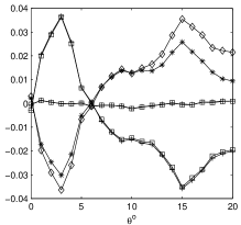
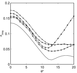
FigureΒ 12 reports various plots of SDs. The continuous line is the result of equationΒ 24 at various ΞΈπœƒ\theta. The other curves are the SD of Ξ΅2,3​(xg​2,3)βˆ’Ξ΅subscriptπœ€23subscriptπ‘₯𝑔23πœ€\varepsilon_{2,3}(x_{g2,3})-\varepsilon and of xg​2,3βˆ’Ξ΅subscriptπ‘₯𝑔23πœ€x_{g2,3}-\varepsilon. For small ΞΈπœƒ\theta the line of is not far from that of Ξ΅2​(xg​2)βˆ’Ξ΅subscriptπœ€2subscriptπ‘₯𝑔2πœ€\varepsilon_{2}(x_{g2})-\varepsilon. For ΞΈ>12βˆ˜πœƒsuperscript12\theta>12^{\circ} the SD of xg​2βˆ’Ξ΅subscriptπ‘₯𝑔2πœ€x_{g2}-\varepsilon starts to increase abandoning the common trends of the other reconstructions. The origin of this increase is connected to the drastic loss of information of the two strip algorithm that produces a large set of forbidden values around xg​2β‰ˆ0subscriptπ‘₯𝑔20x_{g2}\approx 0. In spite of this, the xg​2subscriptπ‘₯𝑔2x_{g2}-algorithm gives an excellent reconstruction Ξ΅2​(xg​2)subscriptπœ€2subscriptπ‘₯𝑔2\varepsilon_{2}(x_{g2}) with a SD better than the SD of Ξ΅3​(xg​3)βˆ’Ξ΅subscriptπœ€3subscriptπ‘₯𝑔3πœ€\varepsilon_{3}(x_{g3})-\varepsilon.

A sort of saturation effect appears when ΞΈ>12βˆ˜πœƒsuperscript12\theta>12^{\circ} for Ξ΅2​(xg​2)βˆ’Ξ΅subscriptπœ€2subscriptπ‘₯𝑔2πœ€\varepsilon_{2}(x_{g2})-\varepsilon, Ξ΅3​(xg​3)βˆ’Ξ΅subscriptπœ€3subscriptπ‘₯𝑔3πœ€\varepsilon_{3}(x_{g3})-\varepsilon and xg​3βˆ’Ξ΅subscriptπ‘₯𝑔3πœ€x_{g3}-\varepsilon. Part of the trend of the analytical calculationΒ 24 is present in the reconstruction errors up to ΞΈβ‰ˆ12βˆ˜πœƒsuperscript12\theta\approx 12^{\circ}, beyond this value the noise (and the loss of information) dominates and the algorithms tend to loose their relations to the noiseless lossless model.
Refer to caption
Figure 12: Standard deviations for various reconstructions, diamond xg​2subscriptπ‘₯𝑔2x_{g2}, circle Ξ΅2subscriptπœ€2\varepsilon_{2}, crosses xg​3subscriptπ‘₯𝑔3x_{g3}, asterisks Ξ΅3subscriptπœ€3\varepsilon_{3}, continuous line the results of equationΒ 24

7.3 Distributions of Ξ΅2,3βˆ’Ξ΅subscriptπœ€23πœ€\varepsilon_{2,3}-\varepsilon

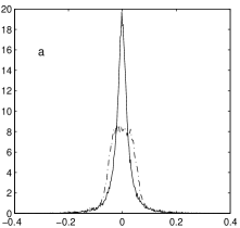
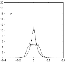
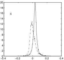
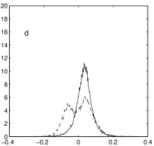
The SD’s are not good parameters to characterize the differences Ξ΅2,3​(xg​2,3)βˆ’Ξ΅subscriptπœ€23subscriptπ‘₯𝑔23πœ€\varepsilon_{2,3}(x_{g2,3})-\varepsilon. Interesting plots are the histograms of the probabilities of Ξ΅2,3​(xg​2,3)βˆ’Ξ΅subscriptπœ€23subscriptπ‘₯𝑔23πœ€\varepsilon_{2,3}(x_{g2,3})-\varepsilon and of xg​2,3βˆ’Ξ΅subscriptπ‘₯𝑔23πœ€x_{g2,3}-\varepsilon. We report them for ΞΈ=0βˆ˜πœƒsuperscript0\theta=0^{\circ} and ΞΈ=5βˆ˜πœƒsuperscript5\theta=5^{\circ} in the figuresΒ 13. The differences Ξ΅2,3​(xg​2,3)βˆ’Ξ΅subscriptπœ€23subscriptπ‘₯𝑔23πœ€\varepsilon_{2,3}(x_{g2,3})-\varepsilon have distributions similar to the Cauchy probability density with a small full width at half maximum (FWHM). It is interesting the dramatic reduction of the FWHM of Ξ΅2,3​(xg​2,3)βˆ’Ξ΅subscriptπœ€23subscriptπ‘₯𝑔23πœ€\varepsilon_{2,3}(x_{g2,3})-\varepsilon respect to the FWHM of xg​2,3βˆ’Ξ΅subscriptπ‘₯𝑔23πœ€x_{g2,3}-\varepsilon al low ΞΈπœƒ\theta. No comparable reduction is observed in the SDs that, excluding the SD of xg​2βˆ’Ξ΅subscriptπ‘₯𝑔2πœ€x_{g2}-\varepsilon, have values and trends similar. The FWHM is an important parameter to describe these distributions. At increasing ΞΈπœƒ\theta, the distributions slowly tend to gaussians.

Refer to caption
Refer to caption
Refer to caption
Refer to caption
Figure 13: Figure (a) is the histogram of Ξ΅2​(xg​2)βˆ’Ξ΅subscriptπœ€2subscriptπ‘₯𝑔2πœ€\varepsilon_{2}(x_{g2})-\varepsilon (continuous line) and of xg​2βˆ’Ξ΅subscriptπ‘₯𝑔2πœ€x_{g2}-\varepsilon (dash-dotted line) for normal strips and ΞΈ=0πœƒ0\theta=0. (b) is the histogram of Ξ΅3​(xg​3)βˆ’Ξ΅subscriptπœ€3subscriptπ‘₯𝑔3πœ€\varepsilon_{3}(x_{g3})-\varepsilon (continuous line) and of xg​3βˆ’Ξ΅subscriptπ‘₯𝑔3πœ€x_{g3}-\varepsilon (dash-dotted line). (c) and (d) are for ΞΈ=5βˆ˜πœƒsuperscript5\theta=5^{\circ}. In (c) it is evident the non zero position of the maximum.

7.4 Error Due to φ​(x)πœ‘π‘₯\varphi(x) Asymmetry

In figureΒ 13 we start to see the effect of the asymmetry of φ​(x)πœ‘π‘₯\varphi(x) in the integration constant of equationΒ 20. For ΞΈ=5βˆ˜πœƒsuperscript5\theta=5^{\circ}, the maximum of the distributions for Ξ΅2,3​(xg​2,3)βˆ’Ξ΅subscriptπœ€23subscriptπ‘₯𝑔23πœ€\varepsilon_{2,3}(x_{g2,3})-\varepsilon is shifted from zero, and all the reconstructed values are shifted accordingly. Even if modest in the scale of the SDs, this shift is of the same order of the FWHM. For the floating strip sensor, the shift can be of the order of the SD, as we will see in the following.
Refer to caption
Refer to caption
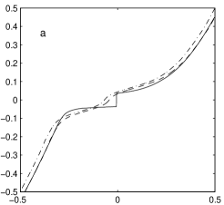
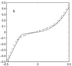
Figure 14: To the left (a) is the plot of xg​2subscriptπ‘₯𝑔2x_{g2} vs Ξ΅2​(xg​2)subscriptπœ€2subscriptπ‘₯𝑔2\varepsilon_{2}(x_{g2}) (dash-dot line) and xg​2subscriptπ‘₯𝑔2x_{g2} noiseless vs. Ξ΅πœ€\varepsilon (solid line) for ΞΈ=5oπœƒsuperscript5π‘œ\theta=5^{o}, the two curves do not coincide as in figureΒ 8, the dashed line is xg​2subscriptπ‘₯𝑔2x_{g2} vs Ξ΅2r​(xg​2)superscriptsubscriptπœ€2π‘Ÿsubscriptπ‘₯𝑔2\varepsilon_{2}^{r}(x_{g2}) corrected as explained in the following. This curve has large overlaps with the noiseless one. To the right (b) the plots of xg​3subscriptπ‘₯𝑔3x_{g3} versus Ξ΅3​(xg​3)subscriptπœ€3subscriptπ‘₯𝑔3\varepsilon_{3}(x_{g3}) (dash dot line) and of xg​3subscriptπ‘₯𝑔3x_{g3} noiseless versus Ξ΅πœ€\varepsilon (solid line) and xg​3subscriptπ‘₯𝑔3x_{g3} vs Ξ΅3r​(xg​3)superscriptsubscriptπœ€3π‘Ÿsubscriptπ‘₯𝑔3\varepsilon_{3}^{r}(x_{g3}) (dashed line)

FigureΒ 14 illustrates the origin of the shift in the maximum of the Ξ΅2,3​(xg​2,3)βˆ’Ξ΅subscriptπœ€23subscriptπ‘₯𝑔23πœ€\varepsilon_{2,3}(x_{g2,3})-\varepsilon probabilities. The lines xg​2,3​(Ξ΅2,3)subscriptπ‘₯𝑔23subscriptπœ€23x_{g2,3}(\varepsilon_{2,3}) do not overlap with the noiseless xg​2,3​(Ξ΅)subscriptπ‘₯𝑔23πœ€x_{g2,3}(\varepsilon), as we have for ΞΈ=0πœƒ0\theta=0, they are shifted to right by a small quantity, thus the reconstructed values Ξ΅2,3​(xg​2,3)subscriptπœ€23subscriptπ‘₯𝑔23\varepsilon_{2,3}(x_{g2,3}) of the events, the maximum and the mean values of Ξ΅2,3​(xg​2,3)βˆ’Ξ΅subscriptπœ€23subscriptπ‘₯𝑔23πœ€\varepsilon_{2,3}(x_{g2,3})-\varepsilon. The corrections, we are going to define, will rigenerate the overlaps. Having to work with mean values, definitions are necessary:

M​Ρ2,3=βˆ‘j=1NΞ΅2,3​(xg​2,3​(j))βˆ’Ξ΅β€‹(j)N𝑀subscriptπœ€23superscriptsubscript𝑗1𝑁subscriptπœ€23subscriptπ‘₯𝑔23π‘—πœ€π‘—π‘\displaystyle M\varepsilon_{2,3}=\sum_{j=1}^{N}\frac{\varepsilon_{2,3}(x_{g2,3}(j))-\varepsilon(j)}{N} (25)
Mx​2,3,4l=βˆ‘j=1Nxg​2,3,4​(j)βˆ’ΞΌβ€‹(j)N,superscriptsubscript𝑀π‘₯234𝑙superscriptsubscript𝑗1𝑁subscriptπ‘₯𝑔234π‘—πœ‡π‘—π‘\displaystyle M_{x2,3,4}^{l}=\sum_{j=1}^{N}\frac{x_{g2,3,4}(j)-\mu(j)}{N},

where μ​(j)πœ‡π‘—\mu(j) is the position of the center of the strip with the maximum signal for the event j𝑗j. The term xg​n​(j)βˆ’ΞΌβ€‹(j)subscriptπ‘₯π‘”π‘›π‘—πœ‡π‘—x_{gn}(j)-\mu(j) is the COG of the event j𝑗j in the virtual strip we used to calculate the probability distribution. We call local these averages to stress their independence from the true event position.
Refer to caption
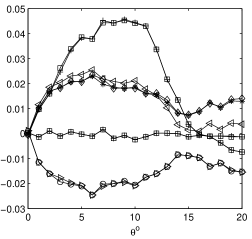
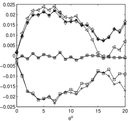
Figure 15: Plots of mean values in function of ΞΈπœƒ\theta. Diamonds Mx​4lsuperscriptsubscript𝑀π‘₯4𝑙M_{x4}^{l}, asterisks Mx​3lsuperscriptsubscript𝑀π‘₯3𝑙M_{x3}^{l}, triangles Mx​2lsuperscriptsubscript𝑀π‘₯2𝑙M_{x2}^{l}, crosses M​Ρ2𝑀subscriptπœ€2M\varepsilon_{2}, squares M​Ρ3𝑀subscriptπœ€3M\varepsilon_{3}, the lines around zero are M​Ρ3r𝑀superscriptsubscriptπœ€3π‘ŸM\varepsilon_{3}^{r} and M​Ρ2r𝑀superscriptsubscriptπœ€2π‘ŸM\varepsilon_{2}^{r}

FigureΒ 15 summarizes the ΞΈπœƒ\theta-dependent averages: M​Ρ2𝑀subscriptπœ€2M\varepsilon_{2}, M​Ρ3𝑀subscriptπœ€3M\varepsilon_{3}, Mx​2lsuperscriptsubscript𝑀π‘₯2𝑙M_{x2}^{l}, Mx​3lsuperscriptsubscript𝑀π‘₯3𝑙M_{x3}^{l} and Mx​4lsuperscriptsubscript𝑀π‘₯4𝑙M_{x4}^{l}. The figure is complex to read in detail. But, at first glance, two almost symmetric group of lines respect to zero are evident. The lines for negative values are the systematic errors M​Ρ2𝑀subscriptπœ€2M\varepsilon_{2} and M​Ρ3𝑀subscriptπœ€3M\varepsilon_{3}. The lines for positive values are the averages Mx​2lsuperscriptsubscript𝑀π‘₯2𝑙M_{x2}^{l}, Mx​3lsuperscriptsubscript𝑀π‘₯3𝑙M_{x3}^{l} and Mx​4lsuperscriptsubscript𝑀π‘₯4𝑙M_{x4}^{l}. The lines (overlapped) around zero are the corrected M​Ρ2𝑀subscriptπœ€2M\varepsilon_{2} and M​Ρ3𝑀subscriptπœ€3M\varepsilon_{3}. It easy to guess that the sought corrections are near to Mx​2lsuperscriptsubscript𝑀π‘₯2𝑙M_{x2}^{l}, Mx​3lsuperscriptsubscript𝑀π‘₯3𝑙M_{x3}^{l} or Mx​4lsuperscriptsubscript𝑀π‘₯4𝑙M_{x4}^{l}, in fact, the sum of M​Ρ2𝑀subscriptπœ€2M\varepsilon_{2} or M​Ρ3𝑀subscriptπœ€3M\varepsilon_{3} with Mx​3lsuperscriptsubscript𝑀π‘₯3𝑙M_{x3}^{l} or Mx​4lsuperscriptsubscript𝑀π‘₯4𝑙M_{x4}^{l} is around zero. A careful observation shows that Mx​2lsuperscriptsubscript𝑀π‘₯2𝑙M_{x2}^{l} is not a good correction.

Given these empirical evidences, it is important to demonstrate their origin to assure us that no simulation inconsistencies mimic the rule. With this aim, we must go in depth in the reconstruction algorithms to isolate the constants (in average) they contain.

7.5 The Complete φ​(x)πœ‘π‘₯\varphi(x)-Reconstruction Theorem

First of all, we must demonstrate the last element required to complete the reconstruction theorem that evidently emerges from equationsΒ 15 and 20. The steps of this reconstruction are recalled here.

Given a set of noiseless and lossless events, originating by the same φ​(Ξ΅)πœ‘πœ€\varphi(\varepsilon), the COG xgsubscriptπ‘₯𝑔x_{g} (infinite sampling) for each event is calculated and a probability distribution Γ​(xg)Ξ“subscriptπ‘₯𝑔\Gamma(x_{g}) is obtained.

The events are supposed to uniformly illuminate all the strips, and a periodic Ξ“p​(xg)superscriptΓ𝑝subscriptπ‘₯𝑔\Gamma^{p}(x_{g}) (Ξ“p​(xg)=Ξ“p​(xg+L)β€‹βˆ€Lβˆˆβ„€superscriptΓ𝑝subscriptπ‘₯𝑔superscriptΓ𝑝subscriptπ‘₯𝑔𝐿for-all𝐿℀\Gamma^{p}(x_{g})=\Gamma^{p}(x_{g}+L)\ \forall L\in\mathbb{Z}) is generated.

The integration of Ξ“p​(xg)superscriptΓ𝑝subscriptπ‘₯𝑔\Gamma^{p}(x_{g}) gives:

Ρ​(xg)=∫xg0xgΞ“p​(y)​𝑑y+Ρ​(xg0).πœ€subscriptπ‘₯𝑔superscriptsubscriptsuperscriptsubscriptπ‘₯𝑔0subscriptπ‘₯𝑔superscriptΓ𝑝𝑦differential-dπ‘¦πœ€superscriptsubscriptπ‘₯𝑔0\varepsilon(x_{g})=\int_{x_{g}^{0}}^{x_{g}}\Gamma^{p}(y)dy+\varepsilon(x_{g}^{0}). (26)

EquationΒ 26 produces the functions Ρ​(xg)πœ€subscriptπ‘₯𝑔\varepsilon(x_{g}) or xg​(Ξ΅)subscriptπ‘₯π‘”πœ€x_{g}(\varepsilon). The periodicity of Ξ“p​(xg)superscriptΓ𝑝subscriptπ‘₯𝑔\Gamma^{p}(x_{g}) allows the formΒ LABEL:eq:106 of a FS for their differences with the following expressions for Ξ±nsubscript𝛼𝑛\alpha_{n} and Ξ²ksubscriptπ›½π‘˜\beta_{k}:

Ξ±n=βˆ«βˆ’1/2+1/2eβˆ’i​2​π​n​y​(Ρ​(y)βˆ’y)​dysubscript𝛼𝑛superscriptsubscript1212superscripte𝑖2πœ‹π‘›π‘¦πœ€π‘¦π‘¦differential-d𝑦\displaystyle\alpha_{n}=\int_{-1/2}^{+1/2}\mathrm{e}^{-i2\pi ny}(\varepsilon(y)-y)\mathrm{d}y (27)
Ξ²k=βˆ«βˆ’1/21/2(yβˆ’Ξ΅β€‹(y))​eβˆ’i​2​π​k​Ρ​(y)​Γ​(y)​dysubscriptπ›½π‘˜superscriptsubscript1212π‘¦πœ€π‘¦superscripte𝑖2πœ‹π‘˜πœ€π‘¦Ξ“π‘¦differential-d𝑦\displaystyle\beta_{k}=\int_{-1/2}^{1/2}(y-\varepsilon(y))\mathrm{e}^{-i2\pi k\varepsilon(y)}\Gamma(y)\mathrm{d}y

For a normalized non negative φ​(Ξ΅)πœ‘πœ€\varphi(\varepsilon) ( φ​(Ξ΅)=Π​(Ξ΅)​φ​(Ξ΅)πœ‘πœ€Ξ πœ€πœ‘πœ€\varphi(\varepsilon)=\Pi(\varepsilon)\,\varphi(\varepsilon)) and the response function p​(x)=Π​(x)𝑝π‘₯Ξ π‘₯p(x)=\Pi(x), the derivate d​xg​(Ξ΅)/d​Ρdsubscriptπ‘₯π‘”πœ€dπœ€\mathrm{d}x_{g}(\varepsilon)/\mathrm{d}\varepsilon allows the selection of the function φ​(Ξ΅βˆ’1/2)πœ‘πœ€12\varphi(\varepsilon-1/2) :

Π​(Ξ΅βˆ’1/2)​d​xgd​Ρ=φ​(Ξ΅βˆ’1/2).Ξ πœ€12𝑑subscriptπ‘₯π‘”π‘‘πœ€πœ‘πœ€12\Pi(\varepsilon-1/2)\frac{dx_{g}}{d\varepsilon}=\varphi(\varepsilon-1/2). (28)

The limitation of the function φ​(Ξ΅)πœ‘πœ€\varphi(\varepsilon) to have the support less than a strip can be easily overcome given p​(x)=Π​(x)𝑝π‘₯Ξ π‘₯p(x)=\Pi(x). Assembling various strips the support can be extended. This method cannot be used with the response function used in equationΒ 18. Even in this case the function φ​(Ξ΅)πœ‘πœ€\varphi(\varepsilon) can be reconstructed, but its support must be less than half strip.

The equationsΒ 26 andΒ 28 contain the integration constant Ρ​(βˆ’1/2)πœ€12\varepsilon(-1/2). In the simulations, Ρ​(βˆ’1/2)πœ€12\varepsilon(-1/2) is always set equal to βˆ’1/212-1/2, this position is exact for symmetric φ​(Ξ΅)πœ‘πœ€\varphi(\varepsilon). For asymmetric φ​(Ξ΅)πœ‘πœ€\varphi(\varepsilon) the incorrect Ρ​(βˆ’1/2)πœ€12\varepsilon(-1/2) shifts φ​(Ξ΅)πœ‘πœ€\varphi(\varepsilon) by Ρ​(βˆ’1/2)+1/2πœ€1212\varepsilon(-1/2)+1/2 giving an incorrect reconstruction. The exact value Ρ​(βˆ’1/2)πœ€12\varepsilon(-1/2) must be extracted from the data to extend the reconstruction theorem to asymmetrical φ​(Ξ΅)πœ‘πœ€\varphi(\varepsilon).

Identical reasoning can be applied to the conventional Ξ·πœ‚\eta algorithm, here the integration starts from zero, the position Ρ​(0)=0πœ€00\varepsilon(0)=0 is correct for ΞΈ=0πœƒ0\theta=0 and symmetric φ​(Ξ΅)πœ‘πœ€\varphi(\varepsilon). For ΞΈβ‰ 0πœƒ0\theta\neq 0 a non zero constant is required.

The empirical property, evident in figureΒ 15, gives a track to complete the theorem. Due to our definitions, we can write the following relations for the mean value of xgsubscriptπ‘₯𝑔x_{g}:

βˆ«βˆ’1/2+1/2Ξ“p​(xg)​xg​dxg=βˆ«βˆ’1/2+1/2xg​d​Ρ​(xg)d​xg​dxg=βˆ«Ξ΅β€‹(βˆ’1/2)Ρ​(+1/2)xg​(Ξ΅)​dΞ΅superscriptsubscript1212superscriptΓ𝑝subscriptπ‘₯𝑔subscriptπ‘₯𝑔differential-dsubscriptπ‘₯𝑔superscriptsubscript1212subscriptπ‘₯𝑔dπœ€subscriptπ‘₯𝑔dsubscriptπ‘₯𝑔differential-dsubscriptπ‘₯𝑔superscriptsubscriptπœ€12πœ€12subscriptπ‘₯π‘”πœ€differential-dπœ€\int_{-1/2}^{+1/2}\Gamma^{p}(x_{g})x_{g}\mathrm{d}x_{g}=\int_{-1/2}^{+1/2}x_{g}\frac{\mathrm{d}\varepsilon(x_{g})}{\mathrm{d}x_{g}}\mathrm{d}x_{g}=\int_{\varepsilon(-1/2)}^{\varepsilon(+1/2)}x_{g}(\varepsilon)\mathrm{d}\varepsilon (29)

Our assumption about the reconstruction of noiseless and lossless events gives for xg​(Ξ΅)subscriptπ‘₯π‘”πœ€x_{g}(\varepsilon) the equation:

xg​(Ξ΅)=Ξ΅+iβ€‹βˆ‘kβ‰ 0,k=βˆ’βˆž+βˆžΞ¦β€‹(βˆ’2​k​π)​P′​(βˆ’2​k​π)​exp⁑(i​ 2​k​π​Ρ)subscriptπ‘₯π‘”πœ€πœ€π‘–superscriptsubscriptformulae-sequenceπ‘˜0π‘˜Ξ¦2π‘˜πœ‹superscriptPβ€²2π‘˜πœ‹π‘–2π‘˜πœ‹πœ€x_{g}(\varepsilon)=\varepsilon+i\sum_{k\neq 0,k=-\infty}^{+\infty}\Phi(-2k\pi)\mathrm{P}^{\prime}(-2k\pi)\exp(i\,2k\pi\varepsilon) (30)

for a generic uniform and symmetric response function p​(x)𝑝π‘₯p(x), and any normalized φ​(Ξ΅)πœ‘πœ€\varphi(\varepsilon). For non symmetric p​(x)𝑝π‘₯p(x) a constant term must be added.

A fundamental property of equationΒ 30 is the absence of the k=0π‘˜0k=0-term in the sum of exponentials (FS). The integral of xg​(Ξ΅)subscriptπ‘₯π‘”πœ€x_{g}(\varepsilon) on a strip length (the period of the FS) has no contribution from the FS, and equationΒ 29 becomes:

βˆ«Ξ΅β€‹(βˆ’1/2)Ρ​(+1/2)xg​(Ξ΅)​dΞ΅=12​[Ρ​(1/2)2βˆ’Ξ΅β€‹(βˆ’1/2)2]superscriptsubscriptπœ€12πœ€12subscriptπ‘₯π‘”πœ€differential-dπœ€12delimited-[]πœ€superscript122πœ€superscript122\int_{\varepsilon(-1/2)}^{\varepsilon(+1/2)}x_{g}(\varepsilon)\mathrm{d}\varepsilon=\frac{1}{2}[\varepsilon(1/2)^{2}-\varepsilon(-1/2)^{2}] (31)

From the periodicity of xg​(Ξ΅)βˆ’Ξ΅subscriptπ‘₯π‘”πœ€πœ€x_{g}(\varepsilon)-\varepsilon and Ρ​(xg)βˆ’xgπœ€subscriptπ‘₯𝑔subscriptπ‘₯𝑔\varepsilon(x_{g})-x_{g} it follows:

Ρ​(xg)βˆ’xg=Ρ​(xgβˆ’1)βˆ’(xgβˆ’1)Ρ​(1/2)βˆ’1/2=Ρ​(βˆ’1/2)+1/2=Ξ”1/2formulae-sequenceπœ€subscriptπ‘₯𝑔subscriptπ‘₯π‘”πœ€subscriptπ‘₯𝑔1subscriptπ‘₯𝑔1πœ€1212πœ€1212subscriptΞ”12\varepsilon(x_{g})-x_{g}=\varepsilon(x_{g}-1)-(x_{g}-1)\ \ \ \ \ \varepsilon(1/2)-1/2=\varepsilon(-1/2)+1/2=\Delta_{1/2}

EquationΒ 29 can be finally expressed as:

βˆ«βˆ’1/2+1/2Ξ“p​(xg)​xg​dxg=Ξ”1/2=Ρ​(βˆ’1/2)+1/2.superscriptsubscript1212superscriptΓ𝑝subscriptπ‘₯𝑔subscriptπ‘₯𝑔differential-dsubscriptπ‘₯𝑔subscriptΞ”12πœ€1212\int_{-1/2}^{+1/2}\Gamma^{p}(x_{g})x_{g}\mathrm{d}x_{g}=\Delta_{1/2}=\varepsilon(-1/2)+1/2. (32)

Ξ”1/2subscriptΞ”12\Delta_{1/2} is just the missing part of the integration constant of equationΒ 26 that completes our initial guess of Ρ​(βˆ’1/2)=βˆ’1/2πœ€1212\varepsilon(-1/2)=-1/2. To conclude, Ξ“p​(xg)superscriptΓ𝑝subscriptπ‘₯𝑔\Gamma^{p}(x_{g}) and its mean value on a strip length allow the reconstruction of asymmetric φ​(Ξ΅)πœ‘πœ€\varphi(\varepsilon).

Excluding equationΒ 28, all the other equations of this section are more general than the needs of φ​(Ξ΅)πœ‘πœ€\varphi(\varepsilon)-reconstruction, and they will be used to correct the systematic error due to the asymmetry in our noisy case.

7.6 Correction of the Systematic Error

As we can see in figureΒ 15, the systematic error is the same for both algorithms. This is not unexpected. In noiseless case, xg​2,3=Β±1/2subscriptπ‘₯𝑔23plus-or-minus12x_{g2,3}=\pm 1/2 is given by the same Ξ΅πœ€\varepsilon-value. If the noise does not contribute in average (and here this is the case for our acceptance of all the energy values corrupted by the noise), the missing constant Ρ​(xg​2,3=βˆ’1/2)+1/2πœ€subscriptπ‘₯𝑔231212\varepsilon(x_{g2,3}=-1/2)+1/2 is the same for MΡ​2subscriptπ‘€πœ€2M_{\varepsilon 2} and MΡ​3subscriptπ‘€πœ€3M_{\varepsilon 3}.

A more precise strategy for the correction of Ξ΅2,3subscriptπœ€23\varepsilon_{2,3} can be found studying their common forms. The final position Ξ΅2,3​(j)subscriptπœ€23𝑗\varepsilon_{2,3}(j) of the event j𝑗j is given by:

Ξ΅2,3​(j)=xg​2,3​(j)+βˆ‘k=βˆ’LLΞ±k​(2,3)​ei​2​π​k​xg​2,3​(j)subscriptπœ€23𝑗subscriptπ‘₯𝑔23𝑗superscriptsubscriptπ‘˜πΏπΏsubscriptπ›Όπ‘˜23superscripte𝑖2πœ‹π‘˜subscriptπ‘₯𝑔23𝑗\varepsilon_{2,3}(j)=x_{g2,3}(j)+\sum_{k=-L}^{L}\,\alpha_{k}(2,3)\mathrm{e}^{i2\pi kx_{g2,3}(j)} (33)

where xg​2,3​(j)subscriptπ‘₯𝑔23𝑗x_{g2,3}(j) is the COG of the event j𝑗j in their true positions (more or less near to the maximum signal strip of the event j𝑗j). {Ξ±l​(2,3)}subscript𝛼𝑙23\{\alpha_{l}(2,3)\} are the constants of the FS for Ξ΅2,3subscriptπœ€23\varepsilon_{2,3}. We need the average of Ξ΅2,3​(j)βˆ’Ξ΅β€‹(j)subscriptπœ€23π‘—πœ€π‘—\varepsilon_{2,3}(j)-\varepsilon(j), the averages of Ξ΅2,3​(j)subscriptπœ€23𝑗\varepsilon_{2,3}(j) and xg​2,3​(j)subscriptπ‘₯𝑔23𝑗x_{g2,3}(j) are transparent. Due to the non uniform distribution of xg​nsubscriptπ‘₯𝑔𝑛x_{gn} in the exponents, the average of the FS is more complex. The xg​n​(j)subscriptπ‘₯𝑔𝑛𝑗x_{gn}(j) are in the global reference system, but the shift of the integer μ​(j)πœ‡π‘—\mu(j) does no modify the exponentials. The average over Γ​(xg​n)Ξ“subscriptπ‘₯𝑔𝑛\Gamma(x_{gn}) due to the periodicity of the exponentials gives:

βˆ«βˆ’βˆž+βˆžΞ“β€‹(xg​n)​ei​ 2​π​k​xg​n​dxg​n=βˆ«βˆ’1/2+1/2Ξ“p​(xg​n)​ei​ 2​π​k​xg​n​dxg​n,superscriptsubscriptΞ“subscriptπ‘₯𝑔𝑛superscripte𝑖2πœ‹π‘˜subscriptπ‘₯𝑔𝑛differential-dsubscriptπ‘₯𝑔𝑛superscriptsubscript1212superscriptΓ𝑝subscriptπ‘₯𝑔𝑛superscripte𝑖2πœ‹π‘˜subscriptπ‘₯𝑔𝑛differential-dsubscriptπ‘₯𝑔𝑛\int_{-\infty}^{+\infty}\Gamma(x_{gn})\mathrm{e}^{i\,2\pi kx_{gn}}\mathrm{d}x_{gn}=\int_{-1/2}^{+1/2}\Gamma^{p}(x_{gn})\mathrm{e}^{i\,2\pi kx_{gn}}\mathrm{d}x_{gn}, (34)

but for equationsΒ 19 and Β 22 the average of the FS becomes:

βˆ‘k=βˆ’L+LΞ±kβ€‹βˆ«βˆ’1/2+1/2Ξ“p​(xg​n)​ei​ 2​π​k​xg​n​dxg​n=Ξ±0+βˆ‘k=βˆ’L+LΞ±kβ€‹Ξ±βˆ’k​i​ 2​π​k.superscriptsubscriptπ‘˜πΏπΏsubscriptπ›Όπ‘˜superscriptsubscript1212superscriptΓ𝑝subscriptπ‘₯𝑔𝑛superscripte𝑖2πœ‹π‘˜subscriptπ‘₯𝑔𝑛differential-dsubscriptπ‘₯𝑔𝑛subscript𝛼0superscriptsubscriptπ‘˜πΏπΏsubscriptπ›Όπ‘˜subscriptπ›Όπ‘˜π‘–2πœ‹π‘˜\sum_{k=-L}^{+L}\alpha_{k}\int_{-1/2}^{+1/2}\Gamma^{p}(x_{gn})\mathrm{e}^{i\,2\pi kx_{gn}}\mathrm{d}x_{gn}=\alpha_{0}+\sum_{k=-L}^{+L}\alpha_{k}\alpha_{-k}i\,2\pi k. (35)

The bilinear term in Ξ±ksubscriptπ›Όπ‘˜\alpha_{k} is zero due to the kπ‘˜k-antisymmetry of its elements, and the average M​Ρ2,3𝑀subscriptπœ€23M\varepsilon_{2,3} is:

M​Ρ2,3=Ξ±0​(2,3)+βˆ‘j=1Nxg​2,3​(j)βˆ’Ξ΅β€‹(j)N=Ξ±0​(2,3)+Mx​2,3l+βˆ‘j=1Nμ​(j)βˆ’Ξ΅β€‹(j)N𝑀subscriptπœ€23subscript𝛼023superscriptsubscript𝑗1𝑁subscriptπ‘₯𝑔23π‘—πœ€π‘—π‘subscript𝛼023superscriptsubscript𝑀π‘₯23𝑙superscriptsubscript𝑗1π‘πœ‡π‘—πœ€π‘—π‘M\varepsilon_{2,3}=\alpha_{0}(2,3)+\sum_{j=1}^{N}\frac{x_{g2,3}(j)-\varepsilon(j)}{N}=\alpha_{0}(2,3)+M_{x2,3}^{l}+\sum_{j=1}^{N}\frac{\mu(j)-\varepsilon(j)}{N} (36)

Recalling the formΒ LABEL:eq:265b of Ξ±0subscript𝛼0\alpha_{0} for any algorithm, the integration on a triangle gives:

Ξ±0=βˆ«βˆ’1/2+1/2dy​[βˆ«βˆ’1/2ydy′​Γp​(yβ€²)βˆ’y]βˆ’12=βˆ’βˆ«βˆ’1/21/2dy′​Γp​(yβ€²)​yβ€²subscript𝛼0superscriptsubscript1212differential-d𝑦delimited-[]superscriptsubscript12𝑦differential-dsuperscript𝑦′superscriptΓ𝑝superscript𝑦′𝑦12superscriptsubscript1212differential-dsuperscript𝑦′superscriptΓ𝑝superscript𝑦′superscript𝑦′\alpha_{0}=\int_{-1/2}^{+1/2}\mathrm{d}y[\int_{-1/2}^{y}\mathrm{d}y^{\prime}\Gamma^{p}(y^{\prime})-y]-\frac{1}{2}=-\int_{-1/2}^{1/2}\mathrm{d}y^{\prime}\Gamma^{p}(y^{\prime})y^{\prime} (37)

In the simulations (and in the data) Ξ±lsubscript𝛼𝑙\alpha_{l}, Mx​2,3lsuperscriptsubscript𝑀π‘₯23𝑙M_{x2,3}^{l} and M​Ρ2,3𝑀subscriptπœ€23M\varepsilon_{2,3} are stochastic variables fluctuating around their mean values, and the following equalities can experience fluctuations due to the statistics:

Ξ±0​(2,3)=βˆ’Mx​2,3lβ‡’M​Ρ2,3=βˆ‘j=1Nμ​(j)βˆ’Ξ΅β€‹(j)Nformulae-sequencesubscript𝛼023superscriptsubscript𝑀π‘₯23𝑙⇒𝑀subscriptπœ€23superscriptsubscript𝑗1π‘πœ‡π‘—πœ€π‘—π‘\alpha_{0}(2,3)=-M_{x2,3}^{l}\ \ \ \ \Rightarrow\ \ \ M\varepsilon_{2,3}=\sum_{j=1}^{N}\frac{\mu(j)-\varepsilon(j)}{N} (38)

Any reference to the used algorithm disappears in the expression of M​Ρ2,3𝑀subscriptπœ€23M\varepsilon_{2,3} and M​Ρ2β‰ˆM​Ρ3𝑀subscriptπœ€2𝑀subscriptπœ€3M\varepsilon_{2}\approx M\varepsilon_{3}. The relation Ξ±0​(2,3)=βˆ’Mx​2,3lsubscript𝛼023superscriptsubscript𝑀π‘₯23𝑙\alpha_{0}(2,3)=-M_{x2,3}^{l} must be handled with care. Different probability distributions are present in the two sides: Ξ±0​(2,3)subscript𝛼023\alpha_{0}(2,3) is defined on a period of the periodic Ξ“p​(xg​2,3)superscriptΓ𝑝subscriptπ‘₯𝑔23\Gamma^{p}(x_{g2,3}), Mx​2,3lsuperscriptsubscript𝑀π‘₯23𝑙M_{x2,3}^{l} is defined on Γ​(xg​2,3)Ξ“subscriptπ‘₯𝑔23\Gamma(x_{g2,3}). These differences are negligible in our simulations of xg​2,3subscriptπ‘₯𝑔23x_{g2,3}, but for xg​4subscriptπ‘₯𝑔4x_{g4} it is large and the systematic error of Ξ΅4subscriptπœ€4\varepsilon_{4} is different from that of Ξ΅2,3subscriptπœ€23\varepsilon_{2,3}.

The correction of M​Ρ2,3𝑀subscriptπœ€23M\varepsilon_{2,3} is obtained recalling equationΒ 30, that for an infinite sampling gives (for asymmetric p​(x)𝑝π‘₯p(x) the following integral is equal to the shift of the COG of p​(x)𝑝π‘₯p(x) respect to the strip center) :

βˆ«βˆ’1/21/2(xg​(Ξ΅)βˆ’Ξ΅)​dΞ΅=0β‡’1Nβ€‹βˆ‘j=1Nxg​n​(j)βˆ’Ξ΅β€‹(j)=0superscriptsubscript1212subscriptπ‘₯π‘”πœ€πœ€differential-dπœ€0β‡’1𝑁superscriptsubscript𝑗1𝑁subscriptπ‘₯π‘”π‘›π‘—πœ€π‘—0\int_{-1/2}^{1/2}(x_{g}(\varepsilon)-\varepsilon)\mathrm{d}\varepsilon=0\ \Rightarrow\ \frac{1}{N}\sum_{j=1}^{N}x_{gn}(j)-\varepsilon(j)=0 (39)

where xg​n​(j)subscriptπ‘₯𝑔𝑛𝑗x_{gn}(j) approximate an infinite sampling containing all the signal strips in the event. For θ≀20βˆ˜πœƒsuperscript20\theta\leq 20^{\circ}, xg​4subscriptπ‘₯𝑔4x_{g4} is negligibly different from an infinite sampling and equationΒ 39 can be recast:

βˆ‘j=1Nxg​4​(j)βˆ’ΞΌβ€‹(j)N+βˆ‘j=1Nμ​(j)βˆ’Ξ΅β€‹(j)N=0β†’Mx​4l=βˆ’βˆ‘j=1Nμ​(j)βˆ’Ξ΅β€‹(j)N.formulae-sequencesuperscriptsubscript𝑗1𝑁subscriptπ‘₯𝑔4π‘—πœ‡π‘—π‘superscriptsubscript𝑗1π‘πœ‡π‘—πœ€π‘—π‘0β†’superscriptsubscript𝑀π‘₯4𝑙superscriptsubscript𝑗1π‘πœ‡π‘—πœ€π‘—π‘\sum_{j=1}^{N}\frac{x_{g4}(j)-\mu(j)}{N}+\sum_{j=1}^{N}\frac{\mu(j)-\varepsilon(j)}{N}=0\ \ \ \ \rightarrow\ \ \ \ M_{x4}^{l}=-\sum_{j=1}^{N}\frac{\mu(j)-\varepsilon(j)}{N}. (40)

The required correction is the mean value of xg​4​(j)subscriptπ‘₯𝑔4𝑗x_{g4}(j) in the reference system of the maximum signal strip we used to collect all the events (in principle scattered in all the detector).

In figureΒ 15, we see that even Mx​3lsuperscriptsubscript𝑀π‘₯3𝑙M_{x3}^{l} can be a good correction in many cases.

We pointed out a possible small non zero value of Mx​2,3l+Ξ±0​(2,3)superscriptsubscript𝑀π‘₯23𝑙subscript𝛼023M_{x2,3}^{l}+\alpha_{0}(2,3), for this the complete correction strategy is expressed by the following rule (for the algorithms with two and three strips):

Ξ΅2,3r​(j)=Ξ΅2,3​(j)βˆ’Mx​2,3lβˆ’Ξ±0​(2,3)+Mx​4l.superscriptsubscriptπœ€23π‘Ÿπ‘—subscriptπœ€23𝑗superscriptsubscript𝑀π‘₯23𝑙subscript𝛼023superscriptsubscript𝑀π‘₯4𝑙\varepsilon_{2,3}^{r}(j)=\varepsilon_{2,3}(j)-M_{x2,3}^{l}-\alpha_{0}(2,3)+M_{x4}^{l}. (41)

For Ξ΅4​(j)subscriptπœ€4𝑗\varepsilon_{4}(j) the correction reduces to the subtraction of Ξ±0​(4)=βˆ’Ξ”1/2subscript𝛼04subscriptΞ”12\alpha_{0}(4)=-\Delta_{1/2} as imposed by equationΒ 32 for the infinite sampling .

In figureΒ 14, the dashed lines is obtained shifting Ξ΅2,3​(xg​2,3)subscriptπœ€23subscriptπ‘₯𝑔23\varepsilon_{2,3}(x_{g2,3}) by βˆ’Mx​2,3lβˆ’Ξ±0​(2,3)+Mx​4lsuperscriptsubscript𝑀π‘₯23𝑙subscript𝛼023superscriptsubscript𝑀π‘₯4𝑙-M_{x2,3}^{l}-\alpha_{0}(2,3)+M_{x4}^{l} and the new lines have a better overlap with the noiseless xg​2,3​(Ξ΅)subscriptπ‘₯𝑔23πœ€x_{g2,3}(\varepsilon).

EquationΒ 41 is able to correct algorithms where Ξ±0​(2,3)subscript𝛼023\alpha_{0}(2,3) is widely different from Mx​2,3lsuperscriptsubscript𝑀π‘₯23𝑙M_{x2,3}^{l} as in our application of an aspect of the Ξ·πœ‚\eta-algorithm. In the Ξ·πœ‚\eta-algorithm, the Ξ·πœ‚\eta-values are 0≀η≀10πœ‚10\leq\eta\leq 1, and the integration on Γ​(Ξ·)Ξ“πœ‚\Gamma(\eta) start from zero. For symmetric φ​(x)πœ‘π‘₯\varphi(x), zero is the right integration constant of equationΒ 26, we use this zero constant for Ξ΅2,3subscriptπœ€23\varepsilon_{2,3} at all θ≀20βˆ˜πœƒsuperscript20\theta\leq 20^{\circ}. In figureΒ 16, the systematic error of M​Ρ2,3𝑀subscriptπœ€23M\varepsilon_{2,3} is reported.

Refer to caption
Figure 16: Plots of mean values in function of ΞΈπœƒ\theta. Crosses M​Ρ2𝑀subscriptπœ€2M\varepsilon_{2}, squares M​Ρ3𝑀subscriptπœ€3M\varepsilon_{3}, diamonds Mx​4lsuperscriptsubscript𝑀π‘₯4𝑙M_{x4}^{l}, asterisks Mx​3lsuperscriptsubscript𝑀π‘₯3𝑙M_{x3}^{l}, triangles Mx​2lsuperscriptsubscript𝑀π‘₯2𝑙M_{x2}^{l}. The lines around zero are M​Ρ2r𝑀superscriptsubscriptπœ€2π‘ŸM\varepsilon_{2}^{r} and M​Ρ3r𝑀superscriptsubscriptπœ€3π‘ŸM\varepsilon_{3}^{r}.

Even here M​Ρ2​(ΞΈ)𝑀subscriptπœ€2πœƒM\varepsilon_{2}(\theta) and M​Ρ3​(ΞΈ)𝑀subscriptπœ€3πœƒM\varepsilon_{3}(\theta) are overlapping. An explanation of this can be obtained observing that xg​2=0subscriptπ‘₯𝑔20x_{g2}=0 and xg​3=0subscriptπ‘₯𝑔30x_{g3}=0 are obtained (in average) for the same Ξ΅πœ€\varepsilon-value, the constant required to correct the systematic error. The differences of Ξ±0​(2,3)subscript𝛼023\alpha_{0}(2,3) from βˆ’Mx​2,3lsuperscriptsubscript𝑀π‘₯23𝑙-M_{x2,3}^{l} can be seen by the lowest lines of figureΒ 16, these are M​Ρ2,3βˆ’Ξ±0​(2,3)βˆ’Mx​2,3l𝑀subscriptπœ€23subscript𝛼023superscriptsubscript𝑀π‘₯23𝑙M\varepsilon_{2,3}-\alpha_{0}(2,3)-M_{x2,3}^{l} and are widely different from M​Ρ2,3𝑀subscriptπœ€23M\varepsilon_{2,3}. In this case, the systematic error is larger than the case with the integration starting at βˆ’1/212-1/2.

The overlap of M​Ρ2​(ΞΈ)𝑀subscriptπœ€2πœƒM\varepsilon_{2}(\theta) with M​Ρ3​(ΞΈ)𝑀subscriptπœ€3πœƒM\varepsilon_{3}(\theta) is a special property of the points Ρ​(βˆ’1/2)πœ€12\varepsilon(-1/2) and of Ρ​(0)πœ€0\varepsilon(0), it disappears with a different stating point of the Ξ“p​(xg)superscriptΓ𝑝subscriptπ‘₯𝑔\Gamma^{p}(x_{g})-integration.

7.7 SD for the Floating Strip Side
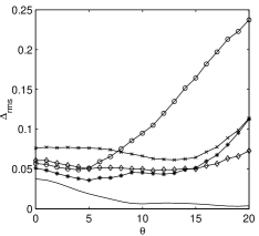
Refer to caption
Figure 17: Trends of the rms errors for various reconstruction algorithms with θ∘superscriptπœƒ\theta^{\circ}: crosses xg​3βˆ’Ξ΅subscriptπ‘₯𝑔3πœ€x_{g3}-\varepsilon, circles xg​2βˆ’Ξ΅subscriptπ‘₯𝑔2πœ€x_{g2}-\varepsilon, diamonds Ξ΅3βˆ’Ξ΅subscriptπœ€3πœ€\varepsilon_{3}-\varepsilon, asterisks Ξ΅2βˆ’Ξ΅subscriptπœ€2πœ€\varepsilon_{2}-\varepsilon, continuous infinite sampling analytical calculation

For ΞΈ=0βˆ˜πœƒsuperscript0\theta=0^{\circ} the SD’s of the various reconstructions are smaller than that of normal strips. At increasing ΞΈπœƒ\theta, the error is almost constant showing that the noise is the dominant factor in reducing the resolution. The SD of xg​2βˆ’Ξ΅subscriptπ‘₯𝑔2πœ€x_{g2}-\varepsilon starts to increase for ΞΈ>5βˆ˜πœƒsuperscript5\theta>5^{\circ}, the loss of information creates a large gap in the xg​2subscriptπ‘₯𝑔2x_{g2}-values around xg​2=0subscriptπ‘₯𝑔20x_{g2}=0. The reconstruction Ξ΅2subscriptπœ€2\varepsilon_{2} is able to keep the error low, but after 15∘superscript1515^{\circ} the SD of Ξ΅3βˆ’Ξ΅subscriptπœ€3πœ€\varepsilon_{3}-\varepsilon is the lowest. The infinite sampling noiseless xgsubscriptπ‘₯𝑔x_{g}-error curve (of equationΒ 24) is always lower than all the other, as we saw in the case of normal strips. The SD of Ξ΅2,3subscriptπœ€23\varepsilon_{2,3} and xg​3subscriptπ‘₯𝑔3x_{g3} show an almost saturating trend up to 15∘superscript1515^{\circ} and after they start to increase.

7.8 Distributions of Ξ΅2,3βˆ’Ξ΅subscriptπœ€23πœ€\varepsilon_{2,3}-\varepsilon

As for the normal strip sensors, the SD (or the rms-error) is not the best parameter to describe the distributions of the differences Ξ΅2,3βˆ’Ξ΅subscriptπœ€23πœ€\varepsilon_{2,3}-\varepsilon. Even for the floating strip sensor, the distributions of the difference Ξ΅2,3βˆ’Ξ΅subscriptπœ€23πœ€\varepsilon_{2,3}-\varepsilon have some similarities with a Cauchy distribution. The histograms of xg​2,3βˆ’Ξ΅subscriptπ‘₯𝑔23πœ€x_{g2,3}-\varepsilon are similar to those of Ξ΅2,3βˆ’Ξ΅subscriptπœ€23πœ€\varepsilon_{2,3}-\varepsilon. This is due to the response function that approximates an ideal detector for signal distributions of this size.

At increasing ΞΈπœƒ\theta a systematic shift of the reconstructed xg​2,3​(Ξ΅2,3)subscriptπ‘₯𝑔23subscriptπœ€23x_{g2,3}(\varepsilon_{2,3}) respect to the noiseless ones is present in figureΒ 19. A shift is evident even in the histograms of the differences Ξ΅2,3βˆ’Ξ΅subscriptπœ€23πœ€\varepsilon_{2,3}-\varepsilon.

At increasing ΞΈπœƒ\theta, figuresΒ 18c and d and figureΒ 19 show shifts similar to those discussed above for the normal strips, and their origin is identical. As anticipated, their order of magnitude is that of the SD.

The histograms of xg​2,3βˆ’Ξ΅subscriptπ‘₯𝑔23πœ€x_{g2,3}-\varepsilon do not show shifts of the mean values, but small shifts are present. The mean value of xgβˆ’Ξ΅subscriptπ‘₯π‘”πœ€x_{g}-\varepsilon is zero only for the infinite sampling case that is well represented by xg​4subscriptπ‘₯𝑔4x_{g4} for θ≀20βˆ˜πœƒsuperscript20\theta\leq 20^{\circ}. In the algorithms with the suppression of signal strips the mean value of xg​nβˆ’Ξ΅subscriptπ‘₯π‘”π‘›πœ€x_{gn}-\varepsilon has a non zero value that can be corrected along the lines of equationΒ 39 andΒ 40.

The corrections of M​Ρ2,3𝑀subscriptπœ€23M\varepsilon_{2,3} are in the form of equationΒ 41. In this sensor side we detected a small signal loss for events around the floating strip, but the corrections work well even here as it can be seen in figureΒ 19. FigureΒ 20 reports M​Ρ2,3​(ΞΈ)𝑀subscriptπœ€23πœƒM\varepsilon_{2,3}(\theta) and Mx​2,3,4l​(ΞΈ)superscriptsubscript𝑀π‘₯234π‘™πœƒM_{x2,3,4}^{l}(\theta), the overlap of M​Ρ2​(ΞΈ)𝑀subscriptπœ€2πœƒM\varepsilon_{2}(\theta) with M​Ρ3​(ΞΈ)𝑀subscriptπœ€3πœƒM\varepsilon_{3}(\theta) indicates that an identical correction is needed and Mx​4lsuperscriptsubscript𝑀π‘₯4𝑙M_{x4}^{l} is the correction. The approximate identity Ξ±0​(2,3)=Mx​2,3lsubscript𝛼023superscriptsubscript𝑀π‘₯23𝑙\alpha_{0}(2,3)=M_{x2,3}^{l} here is well verified.

Refer to caption
Refer to caption
Refer to caption
Refer to caption
Figure 18: To the left (a) it is the histogram of Ξ΅2​(xg​2)βˆ’Ξ΅subscriptπœ€2subscriptπ‘₯𝑔2πœ€\varepsilon_{2}(x_{g2})-\varepsilon (continuous line) and of xg​2βˆ’Ξ΅subscriptπ‘₯𝑔2πœ€x_{g2}-\varepsilon (dash-dotted line) for normal strips and ΞΈ=0βˆ˜πœƒsuperscript0\theta=0^{\circ}. To the right (b) the histogram of Ξ΅3​(xg​3)βˆ’Ξ΅subscriptπœ€3subscriptπ‘₯𝑔3πœ€\varepsilon_{3}(x_{g3})-\varepsilon (continuous line) and of xg​3βˆ’Ξ΅subscriptπ‘₯𝑔3πœ€x_{g3}-\varepsilon (dash-dotted line). c) and d) are for ΞΈ=3βˆ˜πœƒsuperscript3\theta=3^{\circ}. Here, a shift of the maximum respect to zero is evident.
Refer to caption
Refer to caption
Figure 19: To the left (a) is the plot of xg​2subscriptπ‘₯𝑔2x_{g2} vs Ξ΅2​(xg​2)subscriptπœ€2subscriptπ‘₯𝑔2\varepsilon_{2}(x_{g2}) (dash-dot line) and xg​2subscriptπ‘₯𝑔2x_{g2} noiseless vs. Ξ΅πœ€\varepsilon (solid line) for ΞΈ=3βˆ˜πœƒsuperscript3\theta=3^{\circ}, the two curves do not coincide as in figureΒ 8, the dashed line is xg​2subscriptπ‘₯𝑔2x_{g2} vs Ξ΅2r​(xg​2)superscriptsubscriptπœ€2π‘Ÿsubscriptπ‘₯𝑔2\varepsilon_{2}^{r}(x_{g2}) corrected as explained. This curve has large overlaps with the noiseless one. To the right (b) the plots of xg​3subscriptπ‘₯𝑔3x_{g3} versus Ξ΅3​(xg​3)subscriptπœ€3subscriptπ‘₯𝑔3\varepsilon_{3}(x_{g3}) (dash dot line) and of xg​3subscriptπ‘₯𝑔3x_{g3} noiseless versus Ξ΅πœ€\varepsilon (solid line) and xg​3subscriptπ‘₯𝑔3x_{g3} vs Ξ΅3r​(xg​3)superscriptsubscriptπœ€3π‘Ÿsubscriptπ‘₯𝑔3\varepsilon_{3}^{r}(x_{g3}) (dashed line)
Refer to caption
Figure 20: Mean values in function of ΞΈπœƒ\theta, diamonds Mx​4lsuperscriptsubscript𝑀π‘₯4𝑙M_{x4}^{l}, asterisks Mx​2lsuperscriptsubscript𝑀π‘₯2𝑙M_{x2}^{l}, squares M​Ρ3𝑀subscriptπœ€3M\varepsilon_{3}, crosses M​Ρ2𝑀subscriptπœ€2M\varepsilon_{2}, the lines around zero are M​Ρ3c𝑀superscriptsubscriptπœ€3𝑐M\varepsilon_{3}^{c} e M​Ρ2c𝑀superscriptsubscriptπœ€2𝑐M\varepsilon_{2}^{c}.

8 Conclusions

The simulations we realized show useful applications of the results of ref.Β [1]. It turns out sufficiently easy to extract free parameters from the data. The response functions of the strips are optimized for floating strip sensors and normal sensors. For floating strip sensors and signal distributions of this size, the obtained response function can be considered a rough approximation of triangular function with base 2Ο„πœ\tau. This explains the better quality of the position reconstructions of these detectors. The triangular response function (with base 2Ο„πœ\tau) is the simplest response form of a detector (defined ideal in refΒ [1]) where the COG of the hit strips is the exact reconstruction algorithm. The simulations of non orthogonal incoming directions (and asymmetric signals) have immediately underlined the existence of a systematic error in the standard applications of the Ξ·πœ‚\eta algorithm. From the form of our equations, the existence of this type of systematic error is evident from the beginning. The simulations estimate its amplitude, and they give some hint for its suppression. As in the Ξ·πœ‚\eta algorithm, the corrections are extracted from the data. A fundamental step to demonstrate the form of the corrections is the completion of a signal reconstruction theorem for an irregularly sampled, non negative, asymmetric and duration limited signal.

References

  • [1] G. Landi, Nucl. Instr. and Meth. A 485 (2002) 698.
  • [2] G. Landi, Nucl. Instr. and Meth. A 497 (2003) 511.
  • [3] G. Batignani et al., Nucl. Instr. and Meth. A 277 (1989) 147.
  • [4] Acciarri et al., Nucl. Instr. and Meth. A 351 (1994) 300.
  • [5] E. Belau et al., Nucl. Instrum. and Meth. A 214 (1983) 253.
  • [6] R.N. Bracewell, "The Fourier Transform and Its Application" (McGraw-Hill, New York, NY, 1986).
  • [7] D.C. Champeney, "A Handbook of Fourier Theorems" (Cambridge University Press, Cambridge, UK, 1987).
  • [8] I. Abt et al., Nucl. Instrum. and Meth. A 423 (1999) 303.
  • [9] The PAMELA Collaboration in Proceedings XXVI ICRC Salt Lake City Volume OG.4.2.04 1999
  • [10] M. Krammer, H. Pernegger, Nucl. Instr.and Meth. A 397 (1997) 232.