Correlation and Combination of Sets of Parton Distributions

We study the correlation between different sets of parton distributions (PDFs). Specifically, viewing different PDF sets as distinct determinations, generally correlated, of the same underlying physical quantity, we examine the extent to which the correlation between them is due to the underlying data. We do this both for pairs of PDF sets determined using a given fixed methodology, and between sets determined using different methodologies. We show that correlations have a sizable component that is not due to the underlying data, because the data do not determine the PDFs uniquely. We show that the data-driven correlations can be used to assess the efficiency of methodologies used for PDF determination. We also show that the use of data-driven correlations for the combination of different PDFs into a joint set can lead to inconsistent results, and thus that the statistical combination used in constructing the widely used PDF4LHC15 PDF set remains the most reliable method.

1 Uncertainties and correlations of parton distributions

Correlations between parton distribution functions (PDFs) are an important ingredient in the accurate determination of PDFs and their uncertainties, notoriously a current major challenge of contemporary collider precision phenomenology [1]. The correlation between PDFs and physical observables is a tool used to understand both the impact of PDF uncertainties on predictions, and the impact of individual observables on PDF determination, as originally emphasized in Ref. [2], and subsequently exploited for Higgs phenomenology in Sect 3.2 of Ref. [3]. However, more fundamentally, correlations are an integral part of the determination of PDF uncertainties.

Indeed, just as full information on data uncertainties requires knowledge of the experimental covariance matrix, and not just the uncertainty on individual datapoints, full information on PDF uncertainties is encoded in the point-by-point covariance matrix between all pairs of PDFs at any pair of points:

$${\rm Cov}[f_{a}^{p},f_{a}^{q}](x,x^{\prime})=E[f_{a}^{p}(x,Q_{0}^{2})f_{a}^{q}(x^{\prime},Q_{0}^{2})]-E[f_{a}^{p}(x,Q_{0}^{2})]E[f_{a}^{q}(x^{\prime},Q_{0}^{2})],$$ (1)

and associated correlation matrix

$$\rho[f_{a}^{p},f_{a}^{q}](x,x^{\prime})=\frac{{\rm Cov}[f_{a}^{p},f_{a}^{q}](x,x^{\prime})}{\sqrt{{\rm Var}[f_{a}^{p}]{(x)}{\rm Var}[f_{a}^{q}]{(x^{\prime})}}},$$ (2)

where $f^{p}_{a}(x,Q_{0}^{2})$ is the $p$-th PDF with momentum fraction $x$ and a chosen reference scale $Q^{2}_{0}$ in a given PDF set $\Phi_{a}$ and we denote by ${\rm Var}[f^{p}_{a}]$ the variance, i.e. the diagonal element of the covariance matrix

$${\rm Var}[f^{p}_{a}](x)={\rm Cov}[f_{a}^{p},f_{a}^{p}](x,x)=E[f_{a}^{p}(x,Q_{0}^{2})^{2}]-E[f_{a}^{p}(x,Q_{0}^{2})]^{2}.$$ (3)

In what follows, we will use indices $p,q$ to label PDF flavors, and indices $a,b$ to label PDF sets. So $p$ runs over gluon, up, anti-up, down, …, while $a$ runs over NNPDF3.1, NNPDF4.0, MSHT20, CT18…. Henceforth, we will generally consider the case in which $x=x^{\prime}$ and suppress the $x$ and $Q_{0}^{2}$ dependence, so for instance we will write the covariance Eq. (1) as

$${\rm Cov}[f_{a}^{p},f_{a}^{q}]\equiv{\rm Cov}[f_{a}^{p},f_{a}^{q}](x,x)=E[f_{a}^{p}f_{a}^{q}]-E[f^{p}_{a}]E[f_{a}^{q}].$$ (4)

In Eqs. (1-4), $E$ denotes the average over the probability distribution of PDFs; so the PDF covariance matrix ${\rm Cov}[f_{a}^{p},f_{a}^{q}](x,x^{\prime})$ is the second central moment of the joint probability distributions of PDFs. It can be computed in a standard way [4] given a representation of this probability distribution, specifically as a multigaussian in parameter space for a given PDF parametrization, or as a Monte Carlo sample of PDF replicas.

The correlation between PDF flavors Eq. (2) (F-correlation, henceforth) is a standard concept, and it has been widely computed and used. However, one may also define a different kind of correlation: the correlation between PDF sets [5, 6]. Each PDF set is a determination of the same underlying true PDFs. As such, each set can be viewed as a different determination of the same underlying physical quantity. Generally, two determinations of the same quantity are characterized both by an uncertainty, and a correlation between them. In the presence of uncertainties, each determination may be thought of as a random variable. So for a distinct pair of determinations one can define their covariance and correlation, which may then be combined using the standard methodology that is used for the combination of correlated measurements [7, 8]. Indeed, the correlation between two determinations expresses the amount of new information that each determination introduces: two completely independent determinations are fully uncorrelated, while two completely correlated determinations are simply repetitions of the same determination.

Hence we can view any particular PDF set $\Phi_{a}$ containing PDFs $f^{p}_{a}(x,Q_{0}^{2})$ and their uncertainties as an instance of a probability distribution of PDF determinations [9], just like any measurement is an instance of a probability distribution of measurement outcomes. The covariance matrix Eq. (4) can then be viewed as a special case of a more general covariance matrix

$${\rm Cov}[f_{a}^{p},f_{b}^{q}]\equiv{\rm Cov}[f_{a}^{p},f_{b}^{q}](x,x)=E[f_{a}^{p}f^{q}_{b}]-E[f_{a}^{p}]E[f_{b}^{q}]$$ (5)

and corresponding correlation

$$\rho[f_{a}^{p},f_{b}^{q}]=\frac{{\rm Cov}[f_{a}^{p},f_{b}^{q}]}{\sqrt{{\rm Var}[f_{a}^{p}]{\rm Var}[f_{b}^{q}]}},$$ (6)

where again, for simplicity, we only consider the case $x=x^{\prime}$ and suppress the dependence of the PDFs on $x$ and $Q_{0}^{2}$.

Equations (5,6) provide the covariance and correlation, generally between two different PDF flavors, across two different PDF sets, $\Phi_{a}$ and $\Phi_{b}$. We will therefore refer to them as cross-covariance and cross-correlation, respectively. The average in Eq. (5) is now performed over the full probability distribution of PDF sets, i.e. of distinct determinations, of which sets $\Phi_{a}$ and $\Phi_{b}$ are two generic instances. How this might be done in practice is something that we will discuss below.

It is clear that if we take $p=q$ the cross-covariance and cross-correlation Eqs. (5,6) reduce to the covariance and correlation between the two different determinations of PDF $f^{p}$ provided by sets $\Phi_{a}$ and $\Phi_{b}$. Indeed, in this case

$${\rm Cov}[f_{a}^{p},f_{b}^{p}]=E[f_{a}^{p}f^{p}_{b}]-E[f_{a}^{p}]E[f_{b}^{p}],$$ (7)

and the corresponding correlation is

$$\rho[f_{a}^{p},f_{b}^{p}]=\frac{{\rm Cov}[f_{a}^{p},f_{b}^{p}]}{\sqrt{{\rm Var}[f_{a}^{p}]{\rm Var}[f_{b}^{p}]}}.$$ (8)

Equations (7,8) provide respectively the covariance and correlation between two different determinations $f^{p}_{a}(x,Q_{0}^{2})$, $f^{p}_{b}(x,Q_{0}^{2})$ of the $p$-th PDF at point $x$, viewed as two different determinations of the underlying true value, i.e. the covariance and correlation between PDF sets, or S-covariance and S-correlation.

The F-correlation and S-correlation are both special cases of the cross-correlation: the former, specializing to the case in which one compares two different PDFs from the same PDF set, and the latter, specializing to the case in which one compares the same PDF in two different PDF sets. The F-covariance is a covariance in a space of PDFs, within a given set. The S-covariance is instead the covariance in a space of different PDF sets, which is a rather less trivial concept. Specifically, if a Monte Carlo representation is adopted, then a PDF set $\Phi_{a}$ is represented as a set of Monte Carlo PDF replicas $\{f_{a}^{p,(r)}(x,Q_{0}^{2})\}$, and the F-covariance Eq. (1) can be computed by simply averaging over these replicas. In order to achieve something similar for the S-covariance, one would first need to construct replicas that span the space of possible independent determinations of a given PDF — including, say, the results that might have been found by different groups using different methodologies. This is clearly nontrivial.

Elucidating the nontrivial aspects of averaging over the space of PDF determinations is the main goal of this paper.

The reason why the structure of the space of PDF determinations is subtle is that the outcome of a PDF determination does not only depend on the underlying data. Indeed, a PDF determination amounts to the determination of a probability distribution in a space of functions [9], using as input a discrete set of datapoints: hence the outcome is not unique. Specifically, if a very general functional form, such as a neural network, is adopted, then there is an ensemble of best fits of equal quality to fixed underlying data. It has indeed been shown explicitly [10] in the NNPDF framework that if the same data are fitted over and over again, a distribution of best-fit PDFs is obtained, rather than a single answer. In an approach such as the CT18 PDF determination [11] a more restrictive parametrization is adopted and a unique best fit is found, but then the fit is repeated with a large number underlying functional forms also leading to a distribution of best fits.

It is clear that the distribution of best fits for fixed underlying data provides a contribution to the uncertainty (and more generally to the covariance matrix) that is unrelated to the data uncertainty. Accordingly, when computing the S-correlation Eq. (8) there is a contribution to it which comes from integrating over the space of PDFs which correspond to fixed underlying data. But of course, the correlation by construction lies between $-1$ and $+1$, so this also implies that inevitably the data-induced component of the S-correlation is strictly less then one, because it does not include the component that is not data-driven. We will refer to the non-data-driven component as “functional correlation” for short (without committing ourselves to its precise origin). Note that a priori the non-data-driven component also contains uncertainties related to theory choices, such as the value of $\alpha_{s}$, or missing higher order corrections. These are however in principle (though not necessarily in practice) easy to account for by simply varying the relevant parameters, and we will not discuss them here: we will always consider theory assumptions to be fixed.

In the remainder of this paper, we will investigate the relative sizes of the data-driven and functional components. This will be done by computing explicitly the data-driven S-correlation for PDFs determined from the same underlying data. The question we will address is then: how large is the functional component of the correlation, in comparison to the data-driven one — negligible, sizable, perhaps even dominant?

This question is not purely academic, but in fact quite important for applications. First, as mentioned, the F-correlation Eq. (2) is routinely used to estimate the impact of a given dataset on the PDFs. But then, surely knowledge of the size of the data-driven component of the S-correlation is necessary for such an assessment, because it tells us how much the PDF is determined by the underlying data. Furthermore, correlations between independent measurements are normally used when combining different measurements of the same quantity [7]. Combined PDF sets, such as the PDF4LHC15 set [4], can be viewed in a similar way, namely, as the combination of different determinations of the true PDF. At present, these combinations are performed by simply assuming that all PDF sets in the combination are equally likely. However, one might think that they should instead be combined as correlated measurements, and that a determination of the data-driven S-correlation might be useful to this goal [6]. It is then interesting to investigate possible ways to implement such a procedure, and their consequences.

We will answer these questions by computing the data-induced S-correlation explicitly. In Sect. 2 we will present results for the data-driven component of the S-correlation, both between different PDF sets determined from the same underlying data and with the same methodology, and between pairs of PDF sets determined using the same data, but different methodologies. We will use the results to shed light on the origin of the PDF S-correlation, and we will explain how S-correlations can be used as a diagnostic tool when comparing different methodologies. In Sect. 3 we will discuss the implications of our result for the construction of combined PDF sets. After discussing the PDF4LHC15 prescription for the combination of PDF sets in Sect. 3.1, in Sect. 3.2 we will discuss how this could be replaced by a correlated combination, and the consequences of doing so.

2 PDF cross-correlations and S-correlations

2.1 Correlated replicas

Our goal is to compute the cross-correlation between PDF sets, which we can determine from the cross-covariance Eq. (5). We assume that a Monte Carlo representation is used for PDF sets. This assumption is not restrictive, since Hessian PDF sets can be converted into Monte Carlo sets using the methodology of Ref. [12]. A PDF set $\Phi_{a}$ is then represented by a set of $N$ PDF replicas $\{{f_{a}^{p(r)}}:r=1,\ldots N\}$ of the $p$-th PDF flavor $f_{a}^{p}$, that provide an importance sampling of the probability distribution of the the PDF set. We assume for simplicity that the number of PDF replicas $N$ is fixed and sufficiently large that a faithful representation of the underlying probability representation is obtained, and we will provide an estimate of the uncertainty due to finite-size effects. Also, we assume that the PDF sets that are being considered all provide a faithful representation of the underlying data, so that they would for instance pass a closure test [13, 14].

Each replica is equally probable, so replicas are statistically uncorrelated, and estimators of functions of the PDFs are given by simple averages over the replicas,

$$\langle X[f_{a}^{p}]\rangle=\frac{1}{N}\sum_{r=1}^{N}X[{f_{a}^{p}}^{(r)}].$$ (9)

Thus in particular the mean and the F-covariance of the PDF set are given by

$$E[f_{a}^{p}]=\langle f_{a}\rangle,\qquad{\rm Cov}[f_{a}^{p},f_{a}^{q}]=\langle f_{a}^{p}f_{a}^{q}\rangle-\langle f^{p}_{a}\rangle\langle f^{q}_{a}\rangle.$$ (10)

Henceforth, we will use angle brackets to denote the replica average, while the symbol $E$ used in Sect. 2.1 denotes the generic average.

The way PDF replicas are constructed is by first constructing a Monte Carlo representation of the underlying data, i.e. by producing an ensemble of data replicas, such that the ensemble mean reproduces the central value of the original data, and the covariance over the ensemble reproduces the data covariance matrix. These data replicas can then be fitted with whatever methodology is chosen: i.e., a fit to each data replica is performed thereby leading to a best-fit PDF for the given replica. The ensemble of best fits then provides the Monte Carlo representation of PDFs. Note that this can be done in conjunction with any PDF fitting methodology, such as, for example, the MSTW methodology discussed in Ref. [12].

When computing the F-covariance Eqs. (1,10), the same replica is used to determine $f_{a}^{p}$ and $f_{a}^{q}$, so in particular

$$\langle f_{a}^{p}f_{a}^{q}\rangle=\frac{1}{N}\sum_{r=1}^{N}{f_{a}^{p}}^{(r)}{f_{a}^{q}}^{(r)}.$$ (11)

It is important to understand that each PDF replica ${f_{a}^{p}}^{(r)}$ is obtained by fitting to an individual data replica, but, as mentioned, the result of this fit is generally not unique. Indeed, as also mentioned, a distribution of different PDFs is found even when fitting repeatedly the same underlying data. In the NNPDF methodology, that uses a very general neural network as underlying parametrization, this simply follows from the fact that the best-fit neural network trained to fixed underlying data is not unique: each training to fixed underlying data produces a different but equally good answer. In other methodologies this is achieved by considering an ensemble of different functional forms fitted to the same data, each of which gives a different best fit [15, 11, 16]. Clearly, the spread of PDFs fitted to fixed underlying data is completely unrelated to the data uncertainties and correlations. Thus, in order to get the full variance, covariance, ${f_{a}^{p}}^{(r)}$ and ${f_{a}^{q}}^{(r)}$ in Eq. (11) must be PDFs that correspond to the same PDF replica: i.e. to one fixed fit to a fixed data replica.

We would now like to turn to the computation of the S-covariance and S-correlation between two PDF sets $\Phi_{a}$ and $\Phi_{b}$, that we can write as

$${\rm Cov}[f_{a}^{p},f_{b}^{p}] =\langle f_{a}^{p}f_{b}^{p}\rangle-\langle f_{a}^{p}\rangle\langle f_{b}^{p}\rangle,$$ (12)

$$\rho[f_{a}^{p},f_{b}^{p}] =\frac{{\rm Cov}[f_{a}^{p},f_{b}^{p}]}{\sqrt{{\rm Var}[f_{a}^{p}]{\rm Var}[f_{b}^{p}]}}.$$ (13)

Naively, one could think that this might be computed by starting with two sets of PDF replicas representing the two PDF sets, $\{{f_{a}^{p}}^{(r)}\}$ and $\{{f_{b}^{p}}^{(r)}\}$. However it is clear that if these PDF replicas are chosen independently, then the S-covariance, and thus the S-correlation Eq. (8) will always vanish, because the replicas are uncorrelated between sets. Indeed, the same applies to the computation of the standard F-covariance Eq. (10). Namely, if two independent sets of $N$ PDF replicas chosen at random from the same PDF set $\Phi_{a}$ are combined into a set of $2N$ independent PDF replicas then

$$\frac{1}{N}\sum_{r=1}^{N}{f_{a}^{p}}^{(r)}{f_{b}^{p}}^{(N+r)}=\langle f_{a}^{p}\rangle\ \langle f^{p}_{b}\rangle\$$ (14)

and the S-covariance vanishes, where the equality (and thus the vanishing) hold in the large $N$ limit, i.e. within the accuracy of the Monte Carlo representation.

In order to compute the correlation between PDF sets we must thus determine the S-covariance by using PDF replicas that are correlated between PDF set $\Phi_{a}$ and PDF set $\Phi_{b}$. In order to understand what this means, assume for a moment, for the sake of argument, that the data do determine uniquely the best-fit PDF: so that for each data replica there is a unique PDF replica. In this case, when we label each PDF replica ${f_{a}^{p}}^{(r)}$ the index $r$ corresponds uniquely to the specific data replica to which the PDFs have been fitted. Assuming that the two given sets are obtained using two different methodologies, this unique PDF best fit might be slightly different in sets $\Phi_{a}$ and $\Phi_{b}$, so ${f_{a}^{p}}^{(r)}\not={f_{b}^{p}}^{(r)}$. The S-correlation between PDF sets $a$ and $b$ can be computed by simply making sure that the same correlated replica $\{{f_{a}^{p}}^{(r)}\}$ and $\{{f_{b}^{p}}^{(r)}\}$ is used: the cross-covariance Eq. (12) is then generally non-zero, since the PDF replicas are correlated by the choice of the common underlying data replica $r$. This also automatically implies that the PDF set has unit correlation to itself, as it must, because if $a=b$ then the unique answer ${f_{a}^{p}}^{(r)}$ is used in the computation of averages.

However, in actual fact, we know that this is generally not the case: the data replica does not uniquely determine the PDF. So, in a realistic case, for each data replica $r$ and for each PDF set $\Phi_{a}$ there is a distribution of best fits $\{{f_{a}^{p}}^{(r,r^{\prime})}\}$ where now the index $r^{\prime}$ runs over “functional” or methodological replicas: for each data replica, $r$, the index $r^{\prime}$ labels all other aspects that determine the answer. For instance, if parametrization dependence is estimated by varying the functional form, as in Refs. [15, 11, 16], then $r^{\prime}$ would label the different functional forms that are used. If $a=b$, then for fixed $r$ and fixed $r^{\prime}$ the same answer is obtained and the correlation is one: each PDF set has unit correlation to itself. If $a\not=b$, then the S-correlation is found by varying both $r$ and $r^{\prime}$ in a correlated way. If however only $r$ is correlated, and the average over $r^{\prime}$ is performed in an uncorrelated way, the corresponding component of the correlation vanishes according to Eq. (14).

So, if only $r$ is correlated, then the computation provides a non-vanishing component of the S-correlation, namely, its data-driven component, but it misses the functional component, that would also require correlating $r^{\prime}$, and thus it does not give the full correlation. Now, it is clear that if we take $a=b$ in Eq. (12) then the S-covariance reduces to the simple variance and the S-correlation must equal one, at least in the limit of large $N$: it is the correlation of a PDF set to itself. However, if only the data-driven component is included in the computation of the cross-correlation, this consistency check is not satisfied: rather, the result may come out to be less than unity. This deviation from unity tells us, crudely speaking, the extent to which the PDFs are determined by the underlying data. The deviation from one measures the size of the decorrelation due not to having integrated over functional replicas in a correlated way: it tells us how significant the functional component of the S-correlation is.

It is interesting to ask whether the functional component of the cross-correlation could be computed directly. In order to do this, one would need “functional replicas”, namely, one would need to explicitly construct replicas $\{{f_{a}^{p}}^{(r,r^{\prime})}\}$, such that varying the index $r^{\prime}$ fully spans the possible best fits obtained from a fixed underlying data replica $r$. This could perhaps be done when varying aspects of the methodology that influence the final outcome, and that are controlled by a parameter: this parameter would then be fixed to take the same value when computing the S-covariance Eq. (12). We will see an explicit example below, when discussing correlated preprocessing. However, this appears to be nontrivial in general for non-parametric methodology aspects that determine in which of the many equivalent best fits a particular minimization will end up.

In what follows, we will focus on the computation of the data-driven component of the S-correlation. This means that we will use Eq. (12), and we will view the replica index $r$ as an index that labels the underlying pseudodata replica. Then, when comparing two different PDF sets $\Phi_{a}$ and $\Phi_{b}$, the replicas $\{{f_{a}^{p}}^{(r)}\}$ and $\{{f_{b}^{p}}^{(r)}\}$ are fitted to the same underlying data. However, we will also “compare a PDF set $\Phi_{a}$ to itself”. By this, we mean that we will compute the S-correlation (or cross-correlation) by using in Eq. (12) two sets of PDF replicas fitted to the same data replicas using the same methodology, $\{{f_{a}^{p}}^{(r,r^{\prime})}\}$ and $\{{f_{a}^{p}}^{(r,r^{\prime\prime})}\}$, where, as above $r$ labels the data replica while the indices $r^{\prime}$, $r^{\prime\prime}$ span the space of fits to the same data replica. Hence in particular

$$\langle f_{a}^{p}f_{a}^{p}\rangle=\frac{1}{N}\sum_{r=1}^{N}{f_{a}^{p}}^{(r,r^{\prime})}{f_{a}^{p}}^{(r,r^{\prime\prime})}.$$ (15)

In practice, since we have no control on the values of $r^{\prime}$, $r^{\prime\prime}$, $\{{f_{a}^{p}}^{(r,r^{\prime})}\}$ and $\{{f_{a}^{p}}^{(r,r^{\prime\prime})}\}$, are simply two different fits from PDF set $\Phi_{a}$ to the same $r$-th underlying data replica. This is to be contrasted to Eq. (11), used in the computation of the F-correlation, in which the same fit to the same data replica is used: effectively, Eq. (11) corresponds to taking $r^{\prime}=r^{\prime\prime}$ in Eq. (15). We will refer to the situation in which Eq. (15) is used as comparing a PDF set to itself, and we will refer to the resulting correlation as the data-driven component of the correlation.

Figure 1: The kinematic coverage in the $(x,Q^{2})$ plane of the DIS dataset used for the determination of the PDF sets discussed in this paper.

2.2 The data-induced S-correlation and cross-correlation

We compute the data-induced component of the S-correlation, both between a pair of PDF sets determined from the same underlying data using two different methodologies, and between a PDF set and itself, as defined at the end of Sect. 2.1. Specifically, we consider the NNPDF3.1 methodology as presented in Ref. [17], and the NNPDF4.0 methodology recently used for the NNPDF4.0 PDF set [14]. The NNPDF4.0 methodology differs from the NNPDF3.1 methodology mostly because of the choice of PDF parametrization and minimization algorithm, and its main feature is that it is obtained through a hyperoptimization procedure [18]. Here, the details of these two methodologies are not relevant, and it suffices to know that they are both faithful, and compatible with each other (as we will verify explicitly) .

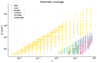
In order to compute the F-correlations and S-correlations shown in this section, we have generated several PDF sets of approximately 1000 PDF replicas each, using the open-source NNPDF code [19]. These PDF replicas have been generated by performing fits to a dataset which consists of the deep-inelastic scattering (DIS) data used for the NNPDF3.1 PDF determination, as listed in Table 1 of Ref. [17]. The kinematic coverage of this data in the $(x,Q^{2})$ plane is shown in Fig. 1. This and all other plots in this paper are produced using validphys [20, 19]. The reasons for choosing a DIS-only dataset are to limit the use of computational resources, as well as to deal with a dataset involving a single, well-understood process, thereby avoiding possible complications related to tensions between data, slow perturbative convergence, and other issues that could obscure our conclusions. Uncertainties on the S-correlations due to the finite size of the replica sample are estimated using a bootstrapping procedure. Further details on the computation of the S-correlation are given in Appendix A.

Figure 2: The gluon PDF as determined with the NNPDF3.1 and NNPDF4.0 methodologies, on a linear (left) and logarithmic (right) scale in $x$.

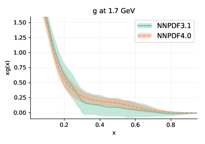
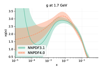
To begin with, we have constructed four PDF sets, all determined from the same underlying data replicas: two using the NNPDF3.1 methodology, and two using the NNPDF4.0 methodology. Whereas a detailed comparison of PDFs produced using the NNPDF4.0 and NNPDF3.1 methodologies is given in Ref. [14], in Fig. 2 we show a representative comparison of the gluon PDF as determined using these two methodologies. The general features of the comparison discussed in Ref. [14] are apparent from this example: namely, first, that results found with either methodology are compatible within uncertainties and central values are generally quite similar, and second, that the NNPDF4.0 methodology leads to rather smaller uncertainties, so generally whereas the NNPDF4.0 central value is within the NNPDF3.1 uncertainty band, the NNPDF3.1 central value is not within the rather smaller NNPDF4.0 uncertainty band.

Figure 3: Distances between central values (top) and uncertainties (bottom) of two PDF sets determined using the NNPDF4.0 methodology. Results are shown both on a logarithmic (left) and linear (right) scale in $x$.

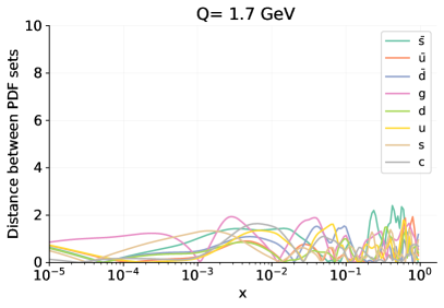
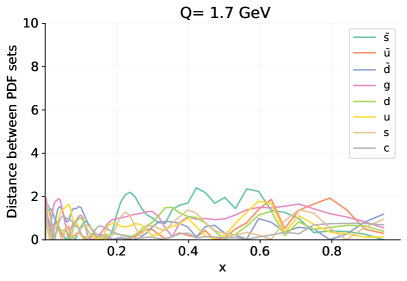
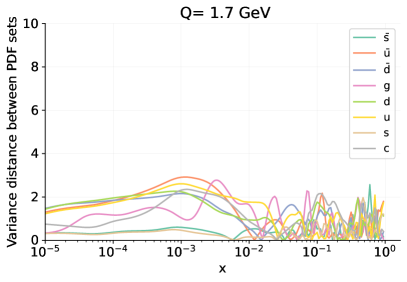
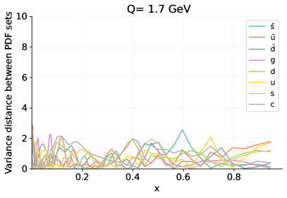
As in all NNPDF determinations, it can be checked explicitly that independently determined PDF replicas all provide a consistent representation of the same underlying probability distribution. Namely, we can check that the standard deviation of the mean of $N_{\rm rep}$ replicas is equal to $\sigma/\sqrt{N_{\rm rep}}$. In order to perform this check, we have generated yet another set of PDF replicas with the NNPDF4.0 methodology, now based on a new set of data replicas. In Fig. 3 we show the distance between the central values and uncertainties of the two different sets of PDF replicas determined using the NNPDF4.0 methodology trained on different sets of data replicas. The distance (defined in Appendix B of Ref. [10]) is the mean square difference of central values in units of the standard deviation of the mean. It is apparent that indeed its value is of order one, as it ought to be. This shows that as the number of replicas increases, both central values and uncertainties of PDFs converge to the mean and standard deviation of the underlying probability distribution.

Having verified that samples of PDF replicas behave as expected, we now proceed to the computation the data-induced component of the S-correlation Eq. (8), as discussed in Sect. 2.1. Results are shown in Fig. 4, where we show the S-correlation between two sets of replicas determined with the NNPDF3.1 methodology (orange); between two sets of replicas determined with the NNPDF4.0 methodology (green); and between a set of replicas determined with the NNPDF3.1 methodology and a set of replicas determined with the NNPDF4.0 methodology (blue). The error bands show the 2$\sigma$ uncertainty due to the finite size of the replica set, estimated using bootstrapping (see Appendix A).

It is apparent from the plots that the data-induced PDF S-correlation drops very quickly to zero outside the data region, as it ought to. For light quarks, the correlations drop to zero for $x\lesssim 10^{-4}$ and $x\gtrsim 0.4$; while the data region is rather smaller for the the gluon and heavy quarks. This is because in a DIS-only PDF determination the gluon PDF is only determined indirectly by scaling violations, while the PDFs for heavier quarks are determined by charged current data, i.e. mostly by fixed-target neutrino DIS data. However, interestingly, even in the middle of the data region the S-correlation of pairs of PDF sets determined using the NNPDF3.1 methodology is typically around 40% and never exceeds 60%. The S-correlation of PDF sets determined using the NNPDF4.0 methodology, in turn, is typically around 60% and never exceeds 80%. The S-correlation between PDF sets determined using the NNPDF3.1 and NNPDF4.0 methodologies, finally, is very similar to the S-correlation between the pair of NNPDF3.1 PDF sets.

As discussed in Sect. 2.1, the deviation from unity of the data-driven S-correlation when comparing of a PDF set to itself is a measure of the size of the functional component of the S-correlation. Both for the NNPDF3.1 and NNPDF4.0 methodologies, this deviation is substantial. Note that, as shown in Fig. 3, any two independent sets of replicas for the same set have the same mean and uncertainty within finite-size fluctuations, and that these fluctuations scale as expected and in particular go to zero in the limit of a large number replicas. Note also that the deviation of the S-correlation from 100% is much larger than the uncertainty due to the finite size of the replica sample, so the correlation loss cannot just be due to an insufficient number of replicas.

The fact that the S-correlation of NNPDF3.1 PDFs is smaller than that of NNPDF4.0 PDFs is consistent with the fact [18, 21, 14] that the NNPDF4.0 methodology leads to smaller uncertainties than the NNPDF3.1 methodology, even though both can be shown to be faithful using closure tests [10, 14]. Indeed, the only way PDF sets determined from the same underlying data can have different uncertainties is if one of the two has a smaller functional (i.e. non-data-driven) component of the uncertainty. But then we would expect that the methodology characterized by a smaller functional uncertainty also has a smaller functional S-correlation: i.e. that it is determined to a greater extent by the underlying data. This is indeed what happens here: NNPDF4.0 has a smaller uncertainty for a fixed dataset, and accordingly a larger S-correlation.

Figure 4: The data-driven component of the S-correlation Eq. (12). Results are shown for all PDF flavors and the gluon. We consider PDF sets determined with the NNPDF3.1 methodology or the NNPDF4.0 methodology, and the three curves shown correspond to comparing pairs of sets with either methodology to themselves (NNPDF3.1: green; NNPDF4.0: orange) or with each other (blue). The shaded band for each curve is the 2$\sigma$ uncertainty due to the finite size of the replica sample, estimated by bootstrapping (see Appendix A). Here and below $\bigcirc$ denotes the operation of comparing quantities computed from two sets of replicas that are correlated by being fitted to the same underlying data.

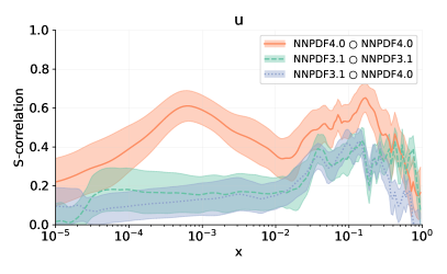
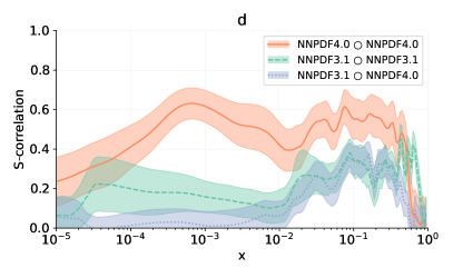
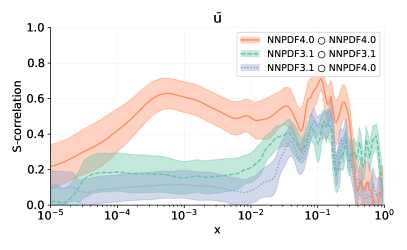
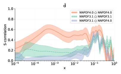
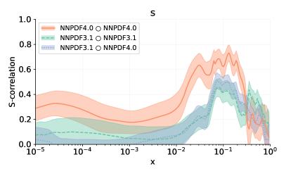
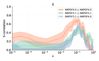
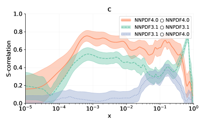
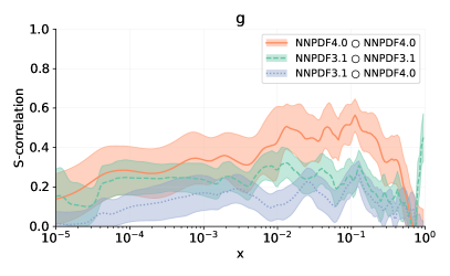
It is interesting to observe that the data-induced component of the S-correlation between NNPDF3.1 and NNPDF4.0 PDFs is almost always similar to that of the PDF set that has the smallest correlation to itself, namely NNPDF3.1 (a possible exception being the charm PDF, which is a special case because in a DIS-only fit it is almost undetermined). This suggests a “weakest-link” explanation: the data are more weakly correlated to NNPDF3.1 than to NNPDF4.0, and so inevitably the data-driven correlation between NNPDF3.1 and NNPDF4.0 is dominated by this weaker correlation. This is apparent, for instance, in the small $x$ region, where the data-driven S-correlation of NNPDF3.1 to itself is significantly weaker than that of NNPDF4.0.

All this suggests that the data-driven component of the S-correlation between PDF sets for a given methodology can be used as a criterion for the assessment of the efficiency of the methodology itself, with the interpretation that a methodology leading to higher cross-correlation is more efficient. Namely, PDFs determined using a methodology characterized by higher S-correlation have a smaller functional component of the S-correlation, i.e. they are to a greater extent determined by the underlying data. So for instance the weaker S-correlation of NNPDF3.1 at small $x$ suggests that in this region the NNPDF3.1 uncertainties could be reduced without loss of accuracy, as is indeed the case [14].

In order to further investigate the functional component of the S-correlation, we have produced sets of PDF replicas in which some methodological choices are correlated or decorrelated. First, we have produced a set of replicas in which preprocessing is also correlated. To understand this, recall that neural networks used to parametrize PDFs include a preprocessing function [18], whose parameters are randomly varied between replicas. We have thus produced a new pair of NNPDF4.0 replicas in which not only the data, but also the preprocessing exponents are correlated: so in Eq. (12), replicas ${f_{a}^{p}(x,Q_{0}^{2})}^{(r)}$ and ${f_{b}^{p}(x,Q_{0}^{2})}^{(r)}$ are not only fitted to the same underlying data, but also have the same value of the preprocessing exponents.

Results are shown in green in Fig. 5, compared to the previous results of Fig. 4, shown in orange. It is clear that in the data region, where the data-induced S-correlation is largest, the extra correlation due to preprocessing is negligible. As PDFs extrapolate further away from the data region, the contribution due to preprocessing is increasingly large: for instance for the gluon at large $x\gtrsim 0.4$ the data-induced correlation rapidly drops to zero as $x\to 1$, but the correlation due preprocessing makes up for the decrease and in fact it somewhat exceeds it as the kinematic boundary at $x=1$ is approached.

Figure 5: The data-driven component of the S-correlation Eq. (12) between PDFs determined with the NNPDF4.0 methodology (same as Fig. 4) compared to the case in which also the preprocessing-induced component is included in the correlation (green), and the case in which the neural network architecture is changed with all other aspects of the methodology kept fixed (blue). Results are shown for the up, anti-down, strange and gluon PDFs.

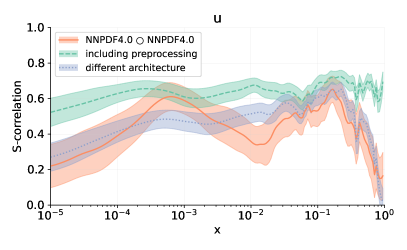
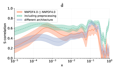
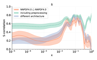
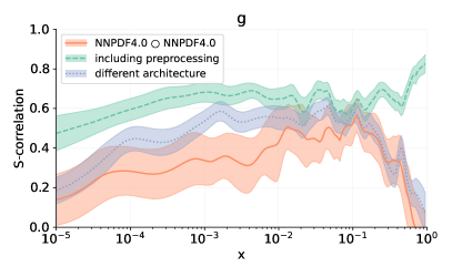
Furthermore, we have produced a PDF set, based on the NNPDF4.0 methodology, but with a different architecture of the neural net, i.e., different number of layers and layer sizes. This is thus effectively a variation of the NNPDF4.0 methodology. Results, also shown in Fig. 5 (in blue), demonstrate that this specific aspect of the methodology has little impact: the S-correlation is essentially the same as in the case where the architecture of the neural networks is the same in the two sets being compared. This shows that these two methodologies lead to very similar results, which in turn suggests that correlating the neural network architecture would have a less significant impact than that of correlating preprocessing.

These two examples illustrate how, at least in principle, all components of the S-correlation could be determined, namely, by correlating all methodological aspects that determine the final result. As already discussed, whereas this is easily done for parametric choices (like the values of the preprocessing exponents), it is rather more difficult for non-parametric aspects, such as, for instance, the choice of minimization settings. These aspects are of course closely tied to the non-uniqueness of the best fit for given data, which leads to functional uncertainties.

Figure 6: Top: comparison of the the data-driven component of the S-correlation Eq. (12) of the up and down PDFs and the up-down cross-correlation Eq. (6). Bottom: comparison between the data-driven component of the up-down cross-correlation Eq. (6) and the standard F-correlation Eq. (2) for the up and down quark PDFs. Results are shown for the NNPDF3.1 (left) and the NNPDF4.0 methodology (right). In all plots (a) and (b) denote two distinct sets of correlated replicas (i.e. fitted to the same underlying data), so (a) $\bigcirc$ (b) denotes the case in which the replicas are correlated but distinct while (a) $\bigcirc$ (a) denotes the case in which the replicas are identical.

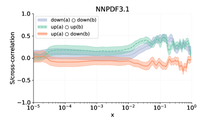
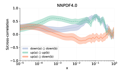
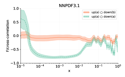
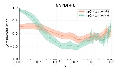
Finally, we compare, for a fixed methodology, the data-driven component of the S-correlation for a pair of PDF flavors, to the cross-correlation between them: in Fig. 6 results are shown for the up and the down PDFs, both for the NNPDF3.1 methodology and the NNPDF4.0 methodology. Clearly, unlike the diagonal S-correlation in the flavor basis Eq. (8), the correlation between two different PDF flavors need not be positive. This is indeed seen in the figure, namely, the up and down PDFs turn out to be anticorrelated at large $x$. Furthermore, one would generally expect any cross-correlation between two different PDF flavors to be weaker than the S-correlation — indeed, if all sources of S-correlation were included, the S-correlation would be 100%. This is again borne out by the explicit computation, that shows that the cross-correlation is generally smaller in modulus than the S-correlation. Note that for the less efficient NNPDF3.1 methodology, for which all S-correlations are smaller, as already discussed, the cross-correlation is accordingly smaller in modulus.

In the same figure we also compare, again for a fixed methodology, the data-induced component of the cross-correlation between the up and down PDFs to the standard F-correlation Eq. (2). Note that if the cross-correlation was entirely data-driven, for a fixed methodology these two quantities would coincide. But in actual fact they differ because in the computation of the F-correlation, Eq. (11) is used (the replicas are fully correlated), while in the computation of the cross-correlation, Eq. (15) is used (the replicas are only correlated through data). Whenever the S-correlation is sizable, the data-induced component of the cross-correlation, and the F-correlation are very close to each other. This means that the functional component of the PDF uncertainty is essentially uncorrelated between different PDFs, i.e. that the standard F-correlation is due to the correlation between the underlying data. This is as one expects, and justifies using PDF correlations to estimate the impact of data uncertainties on PDFs uncertainties and conversely.

However, when the data-induced component of the S-correlation is small, then the S-correlation can differ significantly from the F-correlation. This is clearly seen when comparing the up-down correlation in the region $10^{-4}\lesssim x\lesssim 10^{-2}$ computed with the NNPDF3.1 methodology to that computed with the NNPDF4.0 methodology. With the NNPDF4.0 methodology, the data-driven S-correlation in this region is large, and the standard up-down correlation is quite close to the cross-correlation. With the NNPDF3.1 methodology, on the other hand, the data-driven S-correlation is almost vanishing. This means that, with NNPDF3.1 methodology, PDFs in this region are completely dominated by functional uncertainty, which then screen out the PDF correlation when computing the cross-correlation. In other words, the functional component of the S-correlation (between a PDF and itself) is generally non-negligible, while the functional component of the cross-correlation (between two different PDFs or two different $x$ values) is generally quite small.

3 Combined PDF sets

As already mentioned in Sect. 1, combined PDF sets have been produced [22, 4], with the goal of providing a common, conservative PDF determination. The underlying idea is that so-called “global” PDF sets, namely PDFs determined using the widest possible amount of experimental information available at a given time, differ due to theoretical and methodological assumptions. If these assumptions all satisfy reasonable criteria of reliability, these different PDF determinations are considered to be equally likely, and thus a conservative choice is to combine them into a single determination. One may then reasonably ask whether this combination might be constructed in such a way as to explicitly take account of the cross-correlation between PDF sets.

3.1 The PDF4LHC15 combination

The PDF4LHC15 prescription [4] for combining different PDF sets $\Phi_{a},\,\Phi_{b},\dots$ may be described as follows. All sets being combined are turned into a Monte Carlo representation, as discussed in Sect. 2.1, i.e. each of them is represented by a set of $N$ PDF replicas $\{{f_{i}^{p}}{(r)}:r=1,\ldots N\}$, where the index $i$ runs over the sets that are being combined. The combined set is then defined simply as the union of the replicas in the individual sets: specifically to combine two sets $\Phi_{a}$ and $\Phi_{b}$, we select randomly $\hbox{$\frac{1}{2}$}N$ replicas from each set, and then define the replicas for the combined set $\{F^{p}\}=\{{F^{p}}^{(r)}:r=1,\ldots N\}$ as

$${F^{p}}^{(r)}=\begin{cases}{f_{a}^{p(r)}\qquad\mbox{for $r=1,\ldots,\hbox{$\frac{1}{2}$}N$;}}\\ {f_{b}^{p(r)}\qquad\mbox{for $r=\hbox{$\frac{1}{2}$}N+1,\ldots,N$.}}\end{cases}$$ (16)

The combination assumes that, in the absence of an objective criterion for deciding on the relative probability of the different sets, they are equally probable, and thus that we should take the same number of replicas from each set.

The combined set $\{F^{p}\}$ is then treated in the same way as the individual sets for the calculation of estimators, with the averages taken over all the replicas in the set according to Eq. (9). Thus in particular the mean of any PDF in the combined set is immediately seen to be given by

$$E[F^{p}]=\hbox{$\frac{1}{2}$}(\langle f^{p}_{a}\rangle+\langle f^{p}_{b}\rangle),$$ (17)

while the F-covariance between two PDFs is

$${\rm Cov}[F^{p},F^{q}] = \langle F^{p}F^{q}\rangle-\langle F^{p}\rangle\langle F^{q}\rangle=\hbox{$\frac{1}{2}$}(\langle f^{p}_{a}f^{q}_{a}\rangle+\langle f_{b}^{p}f_{b}^{q}\rangle)-\hbox{$\frac{1}{4}$}(\langle f_{a}^{p}\rangle+\langle f_{b}^{p}\rangle)(\langle f_{a}^{q}\rangle+\langle f^{q}_{b}\rangle)$$ (18)

$$= \hbox{$\frac{1}{2}$}({\rm Cov}[f^{p}_{a},f^{q}_{a}]+{\rm Cov}[f^{p}_{b},f^{q}_{b}])+\hbox{$\frac{1}{4}$}(\langle f^{p}_{a}\rangle-\langle f^{p}_{b}\rangle)(\langle f^{q}_{a}\rangle-\langle f^{q}_{b}\rangle).$$

Thus in the combined set, the central PDF is the mean of the central PDFs in each set (up to the usual statistical uncertainties of order $1/\sqrt{N}$), whereas the uncertainties are always greater than the mean of the uncertainties, the extra term being due to the spread of the central predictions. This is as it should be: when the sets used in the combination disagree, the uncertainty is increased.

The expressions Eqs. (17,18) can be generalized straightforwardly to the combination of $n$ PDF sets, by taking $N/n$ replicas at random from each (always keeping $N\gg n$ of course): then

$$F^{p(r)}=\begin{cases}{f_{a_{1}}^{p(r)}\qquad\mbox{for $r=1,\ldots,\hbox{$\frac{N}{n}$}$;}}\\ {f_{a_{2}}^{p(r)}\qquad\mbox{for $r=\hbox{$\frac{N}{n}$}+1,\ldots,2\hbox{$\frac{N}{n}$}$,}}\\ {\vdots}\qquad\qquad\qquad{\vdots}\\ {f_{a_{n}}^{p(r)}\qquad\mbox{for $r=\hbox{$\frac{n-1}{n}$}N+1,\ldots,N$,}}\end{cases}$$ (19)

and

$$E[F^{p}]=\hbox{$\frac{1}{n}$}\sum_{a}\langle f^{p}_{a}\rangle,\qquad{\rm Cov}[F^{p},F^{q}]=\hbox{$\frac{1}{n}$}\sum_{a}{\rm Cov}[f^{p}_{a},f^{q}_{a}]+\hbox{$\frac{1}{n^{2}}$}\sum_{a\neq b}(\langle f^{p}_{a}\rangle-\langle f^{p}_{b}\rangle)(\langle f^{q}_{a}\rangle-\langle f^{q}_{b}\rangle).$$ (20)

For large $n$ the extra term in the covariance of the combination increases the result according to the covariance of the distribution of central values, since in the pairwise sum there are $n(n-1)$ terms.

The PDF4LHC15 prescription is based on the assumption that the PDF sets that are being combined, viewed as measurements of the true underlying PDF, are all equally likely, which means that they have approximately the same uncertainty and are approximately 100% correlated, i.e. they are not independent. Indeed, independent (uncorrelated or partly correlated) measurements of the same quantity a priori bring in new information on the true value, so the uncertainty on their combination is always smaller or equal to the uncertainty of any of the measurements that are being combined, (see e.g. Ref. [8]), as we shall discuss further in Sect. 3.2 below.

In fact, an important property of the PDF4LHC15 combination prescription is that if the constituent PDF sets $\Phi_{a}$ are perfectly correlated, meaning that taking averages over replicas of the different PDF sets all give the same result, the combination also gives this result. Note that perfectly correlated sets will still be distinct, in the sense that the replicas will not be the same: it is only the averages over the full ensemble of replicas that are the same, in the limit when the number of replicas $N$ becomes very large. An example are the various replica sets considered in Sect. 2.2, all based on the NNPDF4.0 methodology: both the two sets compared in Fig. 3, with replicas based on different underlying data replicas, and those compared in Fig. 4, based on correlated underlying data replicas. For these pairs of sets, $\langle f^{p}_{a}\rangle=\langle f^{p}_{b}\rangle$ for all $a,b$, and ${\rm Cov}[f_{a}^{p},f_{a}^{q}]={\rm Cov}[f_{b}^{p},f_{b}^{q}]$. This is of course true irrespective of the number of sets $n$ used in the combination: it is just the same as when combining several batches of PDF replicas from a given PDF set (such as NNPDF4.0) into a single larger replica set.

To ensure that these assumptions are reasonable, that is, the PDF sets used in the PDF4LHC15 combination are highly correlated, and as such can reasonably be combined by giving equal weight to each set, a number of criteria was adopted [4]:

• Each set is based on a global dataset, and in practice these global datasets are very similar, both in size and content.

• Theoretical calculations are performed to the same order in $\alpha_{s}$, using a VFNS, and benchmarked against one another.

• External parameters such as $\alpha_{s}$ and quark masses are given common values where possible.

• Each PDF determination includes procedural and functional uncertainties in the adopted methodology.

Furthermore, an extensive benchmarking was performed in order to make sure that indeed uncertainties from the various sets were approximately equal, and that these criteria were sufficient to ensure that the PDF sets used in the combination could be be meaningfully assigned equal probability in the combination.

3.2 Correlated PDF combination

It is clear that even though the PDF sets included in the PDF4LHC15 combination are highly correlated, the correlation is manifestly not complete. Even assuming that the benchmarking and parameter settings can achieve complete agreement, there will still be some decorrelation through the choice of global dataset, and in the different methodologies used by the different groups. It has therefore been suggested [6] that a more precise and accurate result might be obtained if different PDFs are combined as independent, partly correlated measurements of the underlying true PDF. The logic is that, even in the presence of a common underlying dataset, each PDF determination, based on a different methodology, might be extracting different information from the data, just like different detectors could provide partly independent though correlated information on the same physical phenomenon. A correlated combination might then be advantageous because it would lead to a more precise and accurate prediction.

Unbiased correlated measurements of the same underlying observable can be combined in a standard way (see e.g. Sect. 7.6 of Ref. [8]). Specifically, viewing the expectation values $E[f_{a}^{p}]$ $a=1,2,\dots$ of PDFs as measurements of an underlying true value, their correlated combination is a weighted average, that we can in turn view as the expectation value of the probability distribution for a combined determination $\tilde{F}^{p}$:

$$E[\tilde{F}^{p}]=\sum_{a}w^{p}_{a}E[f_{a}^{p}],$$ (21)

with weights $w^{p}_{a}$ given by

$$w^{p}_{a}=\frac{\sum_{b}\mathrm{Cov}^{-1}[f_{a}^{p},f_{b}^{p}]}{\sum_{c,d}\mathrm{Cov}^{-1}[f_{c}^{p},f_{d}^{p}]},$$ (22)

where $\mathrm{Cov}^{-1}[f_{a}^{p},f_{b}^{p}]$ is the matrix inverse of the S-covariance. The square uncertainty on the combination Eq. (21) is the variance of the probability distribution of $\tilde{F}^{p}$, given by

$$\mathrm{Var}[\tilde{F}^{p}]=\sum_{a,b}w^{p}_{a}w_{b}^{p}\mathrm{Cov}[f_{a}^{p},f_{b}^{p}].$$ (23)

Of course, all this relies on the assumption that the measurements are unbiased, and that the correlation between them, namely, the S-correlation Eq. (8), can be reliably computed.

Even so, the combination Eq. (21) is subject to several caveats. Specifically, the weights $w^{p}_{a}$ Eq. (22) depend not only on $p$ but also on $x$ because the S-correlation does (recall Eq. (5)), and consequently, the combined PDF Eq. (21) does not automatically satisfy sum rules. Furthermore, for the same reason, the result of the combination will generally depend on the scale at which it is performed, because with $x$-dependent weights even if the PDF sets $f_{a}^{p}$, for each $a$ satisfy QCD evolution equations, the combination does not. Finally, in order to compute physical observables using the combined PDFs, knowledge of the diagonal uncertainty Eq. (23) is not sufficient: rather, the full cross-covariance matrix for all $p,q$ and all $x,y$ would be required. This could be done in principle by sampling the PDFs, computing their F-correlation, and then turning the result into a Hessian representation by using techniques similar to those of Ref. [23]. A way out of all these problems might be to perform the weighted combination Eq. (21) not at the level of PDFs, but rather at the level of physical observables. However, this has the further disadvantage that cross-covariances and weights would have to be re-computed for each new observable.

Be all that as it may, our goal here is not to investigate the most efficient way to implement the weighted combination, but rather, to explore the implications of performing a correlated weighted PDF combination according to Eqs. (21-23). As discussed in Sect. 3.1, in practice the PDF sets in the PDF4LHC15 combination have approximately equal uncertainties. When this is the case, the weights Eq. (22) are all approximately equal, and constant (independent of $x$), and then all the aforementioned problems can be ignored. Indeed, when we combine two PDF sets $\Phi_{a}$ and $\Phi_{b}$ such that ${\rm Var}[f_{a}^{p}]={\rm Var}[f_{b}^{p}]$ the S-covariance is

$$\mathrm{Cov}[f_{a}^{p},f_{b}^{p}]=\big{(}\delta_{ab}+(1-\delta_{ab})\rho[f_{a}^{p},f_{b}^{p}]\big{)}\mathrm{Var}[f_{a}^{p}],$$ (24)

from which it follows, using Eq. (22), that $w_{a}=w_{b}=\hbox{$\frac{1}{2}$}$.

This equal weight situation can be very simply implemented in a Monte Carlo approach, in a completely equivalent way. Indeed, assuming that Monte Carlo replicas are available for two PDFs, $\Phi_{a}$ and $\Phi_{b}$, the correlated combination is found by combining the two sets of replicas into a single replica set given by

$$\tilde{F}^{p(r)}=\hbox{$\frac{1}{2}$}({f_{a}^{p}}^{(r)}+{f_{b}^{p}}^{(r)})$$ (25)

for $r=1,\ldots,N$. Then $E[\tilde{F}^{p}]=\langle F^{p(r)}\rangle=\hbox{$\frac{1}{2}$}(\langle{f_{a}^{p}}^{(r)}\rangle+\langle{f_{b}^{p}}^{(r)}\rangle)$, is in agreement with Eq. (21) when $w_{a}=w_{b}=\hbox{$\frac{1}{2}$}$. The F-covariance Eq. (18) evaluated over the replica set Eq. (25) is now given by

$${\rm Cov}[\tilde{F^{p}},\tilde{F^{q}}] = \langle\tilde{F^{p}}\tilde{F^{q}}\rangle-\langle\tilde{F^{p}}\rangle\langle\tilde{F^{q}}\rangle$$ (26)

$$= \hbox{$\frac{1}{4}$}(\langle f^{p}_{a}f^{q}_{a}\rangle+\langle f^{p}_{b}f^{q}_{b}\rangle+\langle(f^{p}_{a}f_{b}^{q}+(f_{b}^{p}f_{a}^{q})\rangle-\hbox{$\frac{1}{4}$}(\langle f_{a}^{p}\rangle+\langle f_{b}^{p}\rangle)(\langle f_{a}^{q}\rangle+\langle f^{q}_{b}\rangle)$$

$$= \hbox{$\frac{1}{4}$}({\rm Cov}[f^{p}_{a},f^{q}_{a}]+{\rm Cov}[f^{p}_{b},f^{q}_{b}])+\hbox{$\frac{1}{4}$}({\rm Cov}[f^{p}_{a},f^{q}_{b}]+{\rm Cov}[f^{p}_{b},f^{q}_{a}]).$$

Note that when expressed in terms of the replicas from the original sets $\Phi_{a}$ and $\Phi_{b}$ the F-covariance between two PDFs in the combined set now depends on the cross-covariance between the corresponding PDFs of the original sets ${\rm Cov}[f_{a}^{p},f_{b}^{q}]$ Eq. (6). Considering the diagonal case $p=q$ in Eq. (26), the variance of the PDFs of the combined set now depends on the S-correlation, and, using ${\rm Var}[f_{a}^{p}]={\rm Var}[f_{b}^{p}]$, Eq. (26) with $p=q$ reduces to

$${\rm Var}[\tilde{F^{p}}]=\hbox{$\frac{1}{2}$}\left(1+\rho[f^{p}_{a},f^{p}_{b}]\right){\rm Var}[f^{p}_{a}],$$ (27)

which is the same as Eq. (24) when $a=b$.

Using the correlated Monte Carlo approach, the properties of the correlated combination are especially transparent. Specifically, it is clear that the uncertainty computed using Eq. (26) is always smaller than that found using the PDF4LHC15 combination. To see this, note that the correlation $|\rho[f_{a},f_{b}]|\leq 1$ or equivalently $|{\rm Cov}[f_{a},f_{b}]|\leq\sqrt{{\rm Var}[f_{a}]}\sqrt{{\rm Var}[f_{b}]}$. It follows that the square uncertainty on $F^{p}(x,Q_{0}^{2})$ satisfies the inequality

$${\rm Var}[\tilde{F^{p}}]\leq\hbox{$\frac{1}{4}$}({\rm Var}[f^{p}_{a}]+{\rm Var}[f^{p}_{b}])+\hbox{$\frac{1}{2}$}\sqrt{{\rm Var}[f^{p}_{a}]}\sqrt{{\rm Var}[f^{p}_{b}]}\leq\hbox{$\frac{1}{2}$}({\rm Var}[f^{p}_{a}]+{\rm Var}[f^{p}_{b}])\leq{\rm Var}[F^{p}],$$ (28)

where in going from the first to the second inequality we have trivially made use of the fact that $\hbox{$\frac{1}{2}$}(x+y)^{2}\leq x^{2}+y^{2}$, and the third inequality follows from the observation that the second term in Eq. (18) is non-negative.

The second inequality Eq. (28) has the obvious implication that, as already mentioned in Sect. 2.1, and as seen explicitly from Eq. (27), whenever the correlation $\rho[f^{p}_{a},f^{p}_{b}]<1$ the uncertainty of the correlated combination $\tilde{F}^{p}$ is smaller than either of the uncertainties on $f_{a}^{p}$ or $f_{b}^{p}$, that have been assumed to be approximately equal when forming the correlated combination according to Eq. (25), ${\rm Var}[f^{p}_{a}]\approx{\rm Var}[f^{p}_{b}]$.

The third inequality Eq. (28) has the perhaps less obvious implication that even if the two sets are fully correlated, so $\rho[f^{p}_{a},f^{p}_{b}]=1$, the uncertainty on the PDF4LHC15 combination $F^{p}$, can be larger that the uncertainty of either $f_{a}^{p}$ or $f_{b}^{p}$, even though the uncertainty on the correlated combination $\tilde{F^{p}}$ is the same as that on both $f_{a}^{p}$ and $f_{b}^{p}$. This happens whenever the central values of the two sets are not the same $\langle f^{p}_{a}\rangle\not=\langle f^{p}_{b}\rangle$.

This is a situation that the combination formula Eq. (21) cannot accommodate. Indeed, the uncertainty of this correlated combination can never exceed that of the two determinations that are being combined. This follows from the assumption that the two determinations are unbiased estimators of the same underlying true value. Upon these assumptions, unit correlation means that the covariance matrix has a vanishing eigenvalue, so the two determinations have the same central value and uncertainty.

However, it is clearly possible to have two random variables that have unit correlation but do not have the same central value (or uncertainty). In particular the correlation of any two sets of random variables $f^{r}_{1}$ and $f^{r}_{2}$ is invariant under the linear transformations $f^{r}_{1}\to c_{1}f^{r}_{1}+k_{1}$, $f^{r}_{2}\to c_{2}f^{r}_{2}+k_{2}$, for any constants $c_{1},c_{2},k_{1},k_{2}$, which change their mean values and variances. In the Bayesian combination one simply takes the point of view that the two measurements are equally likely determinations of the underlying true quantity, so a priori they might be fully correlated, and yet their mean values and variances might differ. In such a situation, the variance of the PDF4LHC15 combination always comes out larger than those of the determinations that are being combined. So, both the second and the third inequalities Eq. (28) become equalities only if PDF sets $\Phi_{a}$ and $\Phi_{b}$ are identical, i.e. they have the same central value, uncertainty, and unit correlation.

These results are easily generalized to the case of $n$ PDF sets:

$$E[\tilde{F^{p}}]=\frac{1}{n}\sum_{a}\langle f^{p}_{a}\rangle,\qquad{\rm Cov}[\tilde{F^{p}},\tilde{F^{q}}]=\frac{1}{n^{2}}\sum_{a}{\rm Cov}[f^{p}_{a},f^{q}_{a}]+\frac{1}{n^{2}}\sum_{a\neq b}{\rm Cov}[f^{p}_{a},f^{q}_{b}].$$ (29)

In this case

$${\rm Var}[\tilde{F^{p}}]\leq\frac{1}{n^{2}}\sum_{a}{\rm Var}[f^{p}_{a}]+\frac{1}{n^{2}}\sum_{a\neq b}\sqrt{{\rm Var}[f^{p}_{a}]}\sqrt{{\rm Var}[f^{p}_{b}]}\leq\frac{1}{n}\sum_{a}{\rm Var}[f^{p}_{a}]\leq{\rm Var}[F^{p}],$$ (30)

and again equality can only be achieved when there is complete equivalence between all the PDF sets in the combination, i.e. when $f^{p(r)}_{a}=f^{p(r)}_{b}$ for all $r$, $p$ and for all pairs $a,b$. Otherwise, the correlated combination inevitably reduces uncertainties.

Even disregarding the issue related to PDF sets that have different central values despite being very highly correlated, the main problem with the reduction in uncertainty in the correlated combination is that it is reliable only if the cross-correlation has been correctly estimated. In particular, if the cross-correlation is underestimated, then the uncertainty on the combination is underestimated: in the most extreme case, in which two PDFs are fully correlated, but the cross-correlation is incorrectly determined to be very small, the uncertainty on the combination is underestimated by a factor $\sqrt{n}$ (assuming again the uncertainties of the $n$ starting PDFs are approximately the same).

In practice, the problem resides in the construction of the correlated replicas to be used combination Eq. (25): this ought to be done in such a way that the averages over replicas in Eq. (26) lead to a faithful determination of the F-covariance and the S-covariance. As we discussed in Sect. 2.1, if the sets of replicas $\{{f_{a}^{p}}^{(r)}\}$, $\{{f_{b}^{p}}^{(r)}\}$ that are being combined in Eq. (25) are randomly selected from the two sets, then the correlation vanishes regardless of its true value, see Eq. (14). If one selects replicas ${f_{a}^{p}}^{(r)}$, ${f_{a}^{p}}^{(r)}$ that are fitted to the same underlying data replica, then the S-correlation does not vanish, but it is generally underestimated because it only includes its data-driven component, as explicitly shown in Sect. 2.2.

The problem is especially severe when combining $n$ different sets, because in this case underestimating the correlation between each pair of sets will lead to an increasingly large underestimation of the uncertainty on the combination as the number of sets increases. This is because in this case one is effectively assuming that the differences between the different determinations are due to each of them being a partly independent measurement, and as such doing more and more determinations reduces the uncertainty indefinitely.

Figure 7: Check that the Monte Carlo combination Eq. (25) and the correlated combination Eq. (21) of PDF sets yield the same answer. Ten sets sets of 43 NNPDF4.0 PDF replicas are combined : 1) as the correlated weighted average Eq. (21) of the ten result from the ten sets determined using the data-driven component Eq. (12) of the S-correlation (correlated combination); or 2) as the average set of 43 replicas obtained using Eq. (29) from the ten replicas determined from each data replica (Monte Carlo combination). Results are shown for the down (left) and gluon (right) PDF. We show the PDFs normalized to the correlated weighted PDF (top), and the relative 1$\sigma$ uncertainty (bottom).

Figure 8: Comparison of the uncertainty on the correlated PDF combination and the PDF4LHC15 combination for 10 sets of 43 PDF NNPDF4.0 replicas. The correlated combination is obtained as the correlated weighted average of the ten results Eq. (21) (same as shown in Fig. 7); the PDF4LHC15 combination is found by simply combining all replicas in a single 430-replica set.

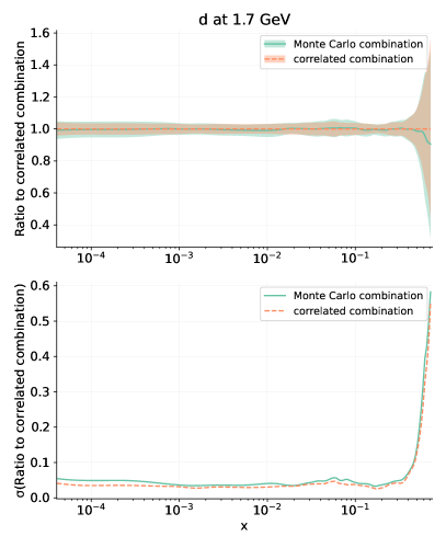
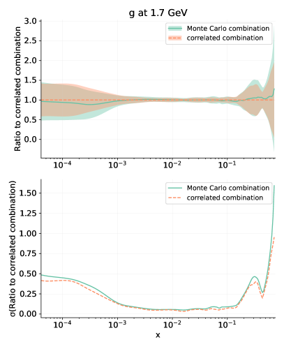
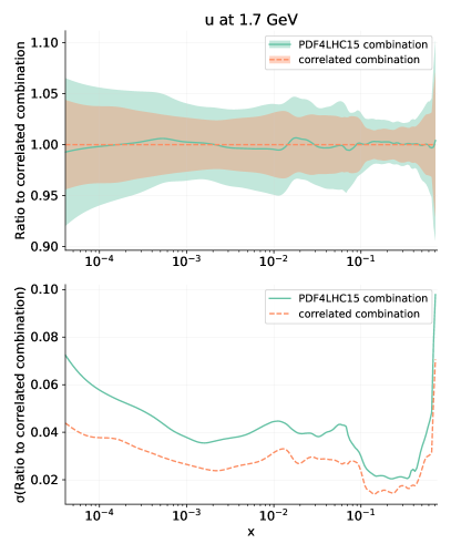
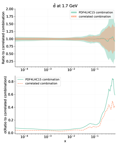
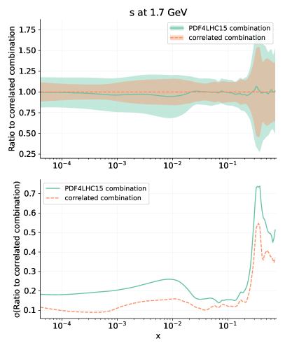
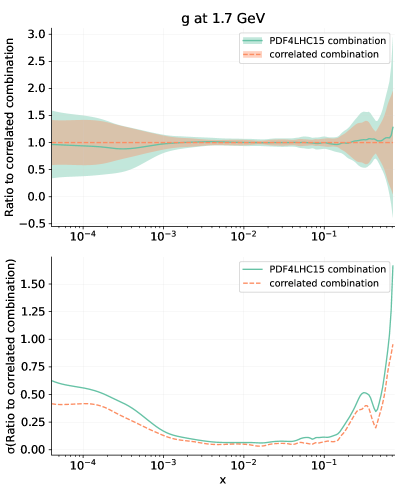
In order to expose the problem, we have considered an implementation of the combination Eq. (21). We have constructed ten sets of $N_{\rm rep}$ PDF replicas, all determined from the same $N_{\rm rep}$ underlying data replicas. In practice we take $N_{\rm rep}=43$ because this is the largest number we got after applying the procedure discussed in Appendix A. We have then computed the ten by ten S-correlation matrix Eq. (12) for each PDF and each $x$ value, and we have combined the ten sets using Eq. (21). We have explicitly checked that this is equivalent to instead using Eq. (29) to combine the ten sets in a single set with 43 replicas. This is demonstrated in Fig. 7 where two representative PDFs determined using either method are compared and seen to agree. This shows that the correlated Monte Carlo combination Eq. (29) is equivalent to the combination using the correlation matrix Eq. (21).

We have then compared this correlated combination to the PDF4LHC15 combination. The latter of course simply consists of putting together all replicas in a single 430 replica PDF set. Results are shown in Fig. 8. It is evident that while the PDF4LHC15 combination gives by construction the correct answer (since in this case the PDF is simply being combined to itself), the correlated combination leads to a rather smaller uncertainty. Clearly this is absurd. The reduction in uncertainty is the consequence of the fact that the S-correlation computed using Eq. (12) only includes the data-induced component. This underestimates the true correlation, because as we have seen in Sect. 2.2 (see in particular Fig. 4) it leads to a S-correlation which is rather lower than one, while in actual fact all these PDFs are fully correlated. The uncertainty reduction is amplified by having combined ten different sets.

We thus see that combining PDFs determined from the same underlying data as if they were correlated measurements leads to an incorrect answer because it neglects the fact that a sizable component of the PDF correlation is not data-driven. Indeed, if one did determine PDF uncertainties in this way, one would reach the paradoxical conclusion that PDF uncertainties can be made smaller at will by simply repeating many times the PDF determination with the same underlying data replicas.

Because of the difficulty in accurately estimating the non-data-driven component of the self-correlation, which is generally significant, this will be the generic scenario. As an especially striking example of this situation, in Fig. 9 we compare the relative uncertainty on the gluon PDF that we find if the gluon is determined using the NNPDF4.0 methodology, the NNPDF3.1 methodology, or the uncorrelated (PDF4LHC15) or correlated combination. As already discussed (see Fig. 2), the uncertainty found using the NNPDF3.1 methodology is rather larger than that found using the NNPDF4.0 methodology. Because, as also discussed, central values are very close, the uncertainty of the PDF4LHC15 combination, Eq. (18) is essentially the average of the uncertainties with the two methodologies. However, the uncertainty on the correlated combination is actually smaller than either of the uncertainties with the two methodologies that are being combined. One would thus reach the paradoxical conclusion that combining PDFs obtained with the more precise NNPDF4.0 methodology with the previous less precise NNPDF3.1 would actually lead to a reduction in uncertainty.

Figure 9: Comparison of the relative uncertainty on the large $x$ gluon PDF determined using (from top to bottom) NNPDF3.1 methodology (purple, dot-dashed), NNPDF3.1 and NNPDF4.0 uncorrelated (PDF4LHC15) combination (green, dotted), NNPDF4.0 methodology (blue, solid), correlated combination (orange, dashes).

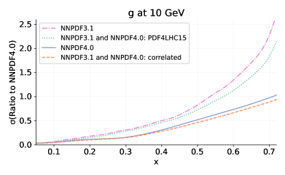
We conclude that a correlated combination inevitably leads to uncertainty underestimation and it cannot be considered as an alternative to the PDF4LHC15 combination, even though the latter might lead to uncertainties that are a little conservative.

4 Conclusions

Treating PDF sets as independent measurements of the same underlying quantity provides a new window into the properties of PDFs, specifically the efficiency of the methodology used to determine the PDFs, and it has allowed us to address in a quantitative way the possibility of performing correlated combinations of PDF sets.

We have studied correlations between pairs of PDF determinations, which we call PDF cross-correlations. By computing these cross-correlations for PDF replicas fitted to the same underlying data replicas, we have shown that the correlation of a PDF set to itself does not come out to be 100% if only the part of the correlation which is due to the underlying data is included. This is due to the fact that a component of the PDF uncertainty, and thus also of the PDF correlation, is not due to the underlying data, but rather of functional origin, namely, related to the fact that the data do not determine uniquely the PDFs. This realization is what allows us to use cross-correlations as a tool in the assessment of the efficiency of the methodology. Indeed, a higher data-driven cross-correlation is an indication of a more efficient methodology, i.e. a methodology that correlates more strongly the PDF to the underlying data.

We have furthermore addressed the feasibility of combining PDF sets as correlated measurements. Specifically, we showed that combining PDFs as correlated measurements will lead the uncertainty of the combination to be underestimated whenever the PDF cross-correlation is underestimated. This will typically happen unless it is possible to determine its functional, non-data-driven component.

In this paper we focused on PDFs produced using the NNPDF framework, in which neural networks are used as basic underlying interpolating functions. The neural network parametrization is redundant, and a best-fit is obtained by not aiming for the minimum of a figure of merit, which would correspond to overlearning, but rather using a variety of techniques such as cross-validation to determine the optimal best fit. In this approach, the presence of a component of the PDF covariance matrix which is not due to the underlying data follows from the fact that this best fit is not unique: an ensemble of best-fit PDFs with non-vanishing covariance is found even when repeatedly fitting the same underlying data.

However, many other modern PDF sets (e.g. CT18 [11] and MSHT20 [16]) rely on parametrizing PDFs with a fixed functional form, for which a unique best fit to any given set of data exists, and is given by the minimum of a figure of merit. Note that this remains true even when used in conjunction with a Monte Carlo approach, in which the fixed functional form is fitted to an ensemble of data replicas [12]. In this case, the functional uncertainty is the result of variations of the functional form, possibly combined with a choice of “tolerance”, whereby an inflation of the $\chi^{2}$ variation corresponding to one-sigma is introduced (either in the data replica generation in a Monte Carlo approach, or in the fitting in a Hessian approach).

A direct computation of the functional contribution to the covariance matrix appears to be very difficult when using the NNPDF approach, and even more challenging when comparing the NNPDF approach to approaches based on an underlying fixed functional form and tolerance. This is due to the difficulty in estimating and even more correlating uncertainties which are not related to the underlying data. In this sense, the results presented here are a first step towards a deeper understanding of origin and meaning of PDF uncertainties.

A general lesson to be learned from this exercise appears to be that if the aim is to improve the accuracy of PDF determination, it is more promising to develop better fitting and diagnostic tools to obtain a more reliable result, than to combine pre-existing determinations in the hope of reducing uncertainties in the combination.

Appendix A Computing cross-correlations in the NNPDF framework

We provide here some details on the computation of the cross-covariance Eq. (12) using NNPDF methodology.

In the NNPDF methodology the data replicas are generated based on a Monte Carlo method with random initialization. Furthermore, input data are split into a training subset used by the optimization algorithm and a validation subset used to validate the optimization [10]. This split is performed randomly for each PDF replica. In order to compute the data-induced component of the cross-correlation therefore we have made sure that the two PDF sets that are being compared are fitted to the same data replicas, with the same training-validation split.

Furthermore, not all fits end up in the final PDF set, but only those that pass post-fit criteria specified in Ref. [10]. Because these criteria are applied a posteriori, it might happen that, for a given underlying data replica, the criteria are only passed by one of the the two PDF replicas that are being compared. For the computation of the cross-correlation, we only include in the final set PDF replicas for which both sets have passed the criteria.

The S-covariance is then computed using Eq. (12), or its obvious generalization in the case of the cross-covariance Eq. (5).

In order to estimate the uncertainty on final results due to the finite size of the replica sample we have used a bootstrapping method [24, 25]. Specifically, we apply a Monte Carlo algorithm to perform a resampling “with replacement” of the PDF replicas. This is of course done synchronously for both PDF sets between which the correlation is calculated. We then calculate the PDF correlation using these resampled PDF sets. This routine is repeated many times to obtain a precise estimate of the standard error of the PDF correlation. The magnitude of the uncertainty decreases with the inverse square root of the number of PDF replicas used to determine the PDF correlation. We have performed this procedure with 200 resampled sets. The value was chosen comparing the 2$\sigma$ standard deviation and the 95% confidence interval, and checking that for any flavor and any value of $x$ they agree.

Finally, we have by default computed the cross-correlation at the scale $Q_{0}=1.7$ GeV, and we have checked that by repeating the computation with different choices of $Q_{0}$ up to 100 GeV results are unchanged.

References

- [1] J. Gao, L. Harland-Lang, and J. Rojo, The Structure of the Proton in the LHC Precision Era, Phys. Rept. 742 (2018) 1–121, [arXiv:1709.04922].
- [2] P. M. Nadolsky et al., Implications of CTEQ global analysis for collider observables, Phys. Rev. D78 (2008) 013004, [arXiv:0802.0007].
- [3] LHC Higgs Cross Section Working Group, S. Dittmaier, et al., Handbook of LHC Higgs Cross Sections: 2. Differential Distributions, CERN-2012-002 (CERN, Geneva, 2012) [arXiv:1201.3084].
- [4] J. Butterworth et al., PDF4LHC recommendations for LHC Run II, J. Phys. G43 (2016) 023001, [arXiv:1510.03865].
- [5] HERAFitter developers’ Team Collaboration, P. Belov et al., Parton distribution functions at LO, NLO and NNLO with correlated uncertainties between orders, Eur. Phys. J. C 74 (2014), no. 10 3039, [arXiv:1404.4234].
- [6] LHC precision EW working group, “Proposal for PDF benchmarking exercise using LHC precision EW data and pseudodata, https://indico.cern.ch/event/775325/contributions/3241729/attachments/1769767/2875062/PDFnote_benchmarking_031218.pdf.” Unpublished note, 2018.
- [7] G. D’Agostini, Bayesian reasoning in data analysis: A critical introduction. World Scientific, 2003.
- [8] G. Cowan, Statistical data analysis. Oxford University Press, 2002.
- [9] W. T. Giele, S. A. Keller, and D. A. Kosower, Parton distribution function uncertainties, hep-ph/0104052.
- [10] NNPDF Collaboration, R. D. Ball et al., Parton distributions for the LHC Run II, JHEP 04 (2015) 040, [arXiv:1410.8849].
- [11] T.-J. Hou et al., New CTEQ global analysis of quantum chromodynamics with high-precision data from the LHC, arXiv:1912.10053.
- [12] G. Watt and R. S. Thorne, Study of Monte Carlo approach to experimental uncertainty propagation with MSTW 2008 PDFs, JHEP 1208 (2012) 052, [arXiv:1205.4024].
- [13] R. D. Ball, Global Parton Distributions for the LHC Run II, Nuovo Cim. C38 (2016), no. 4 127, [arXiv:1507.07891].
- [14] R. D. Ball et al., The Path to Proton Structure at One-Percent Accuracy, arXiv:2109.02653.
- [15] H1 and ZEUS Collaboration, F. Aaron et al., Combined Measurement and QCD Analysis of the Inclusive Scattering Cross Sections at HERA, JHEP 1001 (2010) 109, [arXiv:0911.0884].
- [16] S. Bailey, T. Cridge, L. Harland-Lang, A. Martin, and R. Thorne, Parton distributions from LHC, HERA, Tevatron and fixed target data: MSHT20 PDFs, arXiv:2012.04684.
- [17] NNPDF Collaboration, R. D. Ball et al., Parton distributions from high-precision collider data, Eur. Phys. J. C77 (2017), no. 10 663, [arXiv:1706.00428].
- [18] S. Forte and S. Carrazza, Parton distribution functions, arXiv:2008.12305.
- [19] NNPDF Collaboration, R. D. Ball et al., An open-source machine learning framework for global analyses of parton distributions, arXiv:2109.02671.
- [20] Z. Kassabov, “Reportengine: A framework for declarative data analysis.” https://doi.org/10.5281/zenodo.2571601, Feb., 2019.
- [21] J. Cruz-Martinez, S. Forte, and E. R. Nocera, Future tests of parton distributions, Acta Phys. Polon. B 52 (2021) 243, [arXiv:2103.08606].
- [22] M. Botje et al., The PDF4LHC Working Group Interim Recommendations, arXiv:1101.0538.
- [23] S. Carrazza, S. Forte, Z. Kassabov, J. I. Latorre, and J. Rojo, An Unbiased Hessian Representation for Monte Carlo PDFs, Eur. Phys. J. C75 (2015), no. 8 369, [arXiv:1505.06736].
- [24] B. Efron, Bootstrap Methods: Another Look at the Jackknife, Annals Statist. 7 (1979), no. 1 1–26.
- [25] B. Efron and R. Tibshirani, An introduction to the bootstrap, Statist. Sci. 57 (1986), no. 1 54–75.