Training Deep Neural Networks with Joint Quantization and Pruning of Weights and Activations

Abstract

Quantization and pruning are core techniques used to reduce the inference costs of deep neural networks. State-of-the-art quantization techniques are currently applied to both the weights and activations; however, pruning is most often applied to only the weights of the network. In this work, we jointly apply novel uniform quantization and unstructured pruning methods to both the weights and activations of deep neural networks during training. Using our methods, we empirically evaluate the currently accepted prune-then-quantize paradigm across a wide range of computer vision tasks and observe a non-commutative relationship between pruning and quantization when applied to both the weights and activations of deep neural networks. Informed by these observations, we articulate the non-commutativity hypothesis: for a given deep neural network being trained for a specific task, there exists an exact training schedule in which quantization and pruning can be introduced to optimize network performance. We identify that this optimal ordering not only exists, but also varies across discriminative and generative tasks. Using the optimal training schedule within our training framework, we demonstrate increased performance per memory footprint over existing solutions.

Figure 1: The majority of state-of-the-art frameworks currently default to a “prune-then-quantize" training schedule when jointly applying quantization and pruning to the weights of DNNs (Han et al.,, 2015; Zhao et al., 2019b, ; Yu et al.,, 2020). In such a paradigm, the quantization operator is inactive in the computational order (horizontal flow) until time $t_{+}$, when it is introduced into by the training schedule (vertical flow) to limit precision. Note that in existing approaches, while quantization techniques are applied to both the weights ($\mathbf{w}^{(i)}$) and activations ($\mathbf{h}^{(i)}$) before executing the forward pass of the layer ($L^{(i)}$), pruning is most often only applied to the weights of the network.

1 Introduction

The performance of deep neural networks (DNNs) has been shown to scale with the size of both the training dataset and model architecture (Hestness et al.,, 2017); however, the resources required to deploy large networks for inference can be prohibitive as they often exceed the compute and storage budgets of mobile or edge devices (Han et al.,, 2015; Gale et al.,, 2019). To minimize inference costs, quantization and pruning are widely used techniques that reduce resource requirements by respectively limiting the precision of and removing elements from DNNs.

In this work, we propose a framework for jointly applying novel methods for uniform quantization and unstructured pruning to both the features and weights of DNNs during training. The majority of state-of-the-art techniques for quantization-aware training calculate gradients using the straight-through estimator (STE), which is notoriously sensitive to weight initialization (Yin et al.,, 2019; Gholami et al.,, 2021). To account for this, we propose a modification we refer to as delayed quantization, in which we postpone the STE-based calculations to later training epochs. When applied to generative adversarial networks (GANs) trained on image-to-image translation tasks, we observe a long-tailed distribution of activations, similar to the distribution of weights observed by Wang et al., (2019). To minimize the impact of outliers, we introduce another modification we refer to as saturated quantization, in which we clip the long-tailed distribution of activations based on quantiles determined during training. Finally, we extend the unstructured weight pruning technique proposed by Zhu and Gupta, (2017) to the activation space. To the best of our knowledge, we are the first to thoroughly evaluate the impact of unstructured activation pruning.

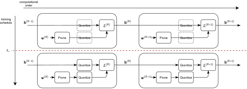
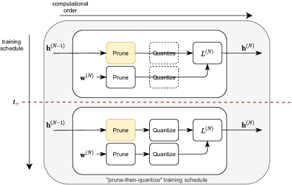
Quantization and pruning techniques are often considered to be independent problems (Paupamah et al.,, 2020; Liang et al.,, 2021); however, recent work has begun to study the joint application of both in a unified scope (Zhao et al., 2019b, ; Yu et al.,, 2020; van Baalen et al.,, 2020). In this work, we aim to more deeply understand the relationship between these optimizations and, in doing so, address two key issues overlooked in previous work: (1) quantization and pruning techniques are often analyzed for either discriminative or generative tasks, rarely both; (2) frameworks for joint quantization and pruning currently default to the “prune-then-quantize” training schedule depicted in Fig. 1 without exploring the alternative. Thus, we evaluate our framework across a wide range of both discriminative and generative tasks and consider the “quantize-the-prune" training schedule in addition to the standard paradigm. In doing so, we observe a non-commutative relationship when applying our novel quantization and pruning methods to both the weights and activations of DNNs. Based on these results, we state the non-commutativity hypothesis.

The Non-Commutativity Hypothesis. For a given deep neural network being trained for a specific task, there exists an exact training schedule in which pruning and quantization can be introduced to optimize the performance of the network on that task.

We empirically evaluate this hypothesis and demonstrate that the optimal ordering in which quantization and pruning can be introduced into the training schedule not only exists but also varies across discriminative and generative tasks. Thus, our results advocate a rethinking of the currently accepted “prune-then-quantize” paradigm. Using the optimal training schedules determined within our framework, we show increased performance per memory footprint over existing solutions.

We summarize our contributions as follows:

1. We propose a framework to train deep neural networks using novel methods for uniform quantization and unstructured pruning on both the weights and activations (Section 3).

2. We demonstrate the non-commutative nature of of quantization and pruning when applied to the weights and activations of DNNs (Section 4.1).

3. We show that our method delivers the best network performance per memory footprint across a wide range of discriminative and generative computer vision tasks when compared to existing state-of-the-art solutions (Section 4.2).

(a)

(b)

Figure 2: As discussed in Section 3, our framework differs from existing solutions in to key ways: (1) we apply unstructured pruning to the activations of the network (yellow); and (2) we enable the consideration of both the standard “prune-then-quantize” training schedule (left) as well as its “quantize-then-prune” analog (right). Using this framework, we empirically evaluate the non-commutativity hypothesis over both discriminative and generative tasks, as discussed in Section 4. Note that under both paradigms, the latent operator (dotted) is activated at time $t_{+}$, at which point both quantization and pruning are applied to both the weights and activations of the DNN.

2 Background

Here, we provide background on the quantization and pruning techniques further detailed in Section 3.

2.1 Uniform Quantization

Quantization minimizes the inference costs by reducing the precision requirements of deep neural networks (DNNs). By uniform quantization, we refer to the process of reducing the precision of all weights and activations to the same number of bits. With energy consumption dominated by data movement, using lower precision representations reduces the energy consumed when running inference by decreasing the memory footprint required to load and store weights and activations while increasing the speed of computations (Horowitz,, 2014; Krishnamoorthi,, 2018). It has been shown that DNNs are resilient to these reductions in precision, and this resilience has been exploited to deploy state-of-the-art models on resource-constrained hardware (Jacob et al.,, 2018; Wu et al.,, 2020; van Baalen et al.,, 2020).

Approaches to quantization are often divided into two categories: post-training quantization and quantization-aware training. Whereas the former applies quantization after a network has been trained, the latter directly considers the loss due to quantization error throughout the training process. It has been shown that quantization-aware training often outperforms post-training quantization  (Krishnamoorthi,, 2018). In Section 3.1, we introduce novel methods for quantization-aware training that uniformly limit the precision of both the weights and activations of DNNs.

2.2 Unstructured Pruning

Pruning is the process of identifying redundant elements to be removed from the computation graph of a DNN. In practice, this is often done by setting the values of the identified elements to zero. The proportion of zero-valued elements is referred to as the network’s sparsity, where a higher value corresponds to fewer non-zero elements (Gale et al.,, 2019).

Pruning techniques are often divided into unstructured or structured approaches which define if and how to impose a pre-defined topology over the computation graph (Gale et al.,, 2019). While structured pruning techniques (e.g., neuron- or channel-pruning) offer simple implementations that efficiently map to modern GPUs, unstructured pruning techniques offer higher compression rates due to their inherent flexibility (Gray et al.,, 2017; Liu et al.,, 2018; Hoefler et al.,, 2021).

Numerous works have studied the benefits of applying unstructured pruning techniques to the weights of DNNs throughout training (Zhu and Gupta,, 2017; Frankle and Carbin,, 2018; Liu et al.,, 2018; Gale et al.,, 2019; Hoefler et al.,, 2021); however, the benefits of also applying unstructured pruning to the activations have yet to be fully explored in the current literature. Existing work on pruning activations has exploited the inherent sparsity patterns in the activations of DNNs to guide post-training model compression techniques (Hu et al.,, 2016) and studied the impact of imposing structured pruning on the activations of DNNs during training (Wang and Zhu,, 2020). However, it has been shown that applying unstructured weight pruning during training achieves higher compression rates while maintaining network performance when compared to post-training or structured techniques (Liu et al.,, 2018; Gale et al.,, 2019). In this work, we are interested in introducing sparsity patterns to guide unstructured pruning of both the weights and activations of DNNs throughout training. To do so, we extend the unstructured pruning techniques proposed by  Zhu and Gupta, (2017) to the activations of DNNs to yield even higher compression rates while maintaining network performance, as further discussed in Section 3.2.

3 Proposed Framework

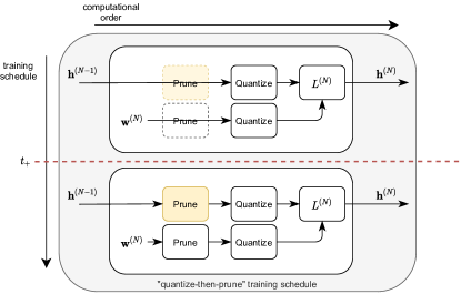
As depicted in Fig. 2, our framework differs from existing solutions in two key ways: (1) we jointly apply our methods for uniform quantization and unstructured pruning to both the weights and activations of DNNs during training; and (2) we enable the consideration of both the standard “prune-then-quantize” training schedule as well as its “quantize-then-prune” analog. As the converse of the “prune-then-quantize” training schedule, the “quantize-then-prune” paradigm deactivates the pruning operator until time $t_{+}$, when it is then introduced into the computational order throughout training. Here, we describe the core methods of our framework.

3.1 Uniform Quantization Method

As shown in Eq. 1, we denote the uniform quantization operator as $Q_{u}(\mathbf{x},d)$, where $\mathbf{x}$ denotes the input to the operator (i.e., weights or activations), $N$ denotes the total number of bits used to represent weights and activations, and $d$ denotes the number of bits used to represent the fractional bits to the right of the decimal.

$$Q_{u}(\mathbf{x},d)=\text{clip}(\lfloor\mathbf{x}\times 2^{d}\rfloor,-2^{N-1},2^{N-1}-1)/2^{d}$$ (1)

To calculate gradients, we use the standard straight-through estimator (STE) given by Eq. 2 which is shown to have superior convergence properties (Hinton et al.,, 2012; Hubara et al.,, 2017). As summarized in Section 1, we introduce delayed and saturated quantization techniques to stabilize STE-based quantization-aware training across both discriminative and generative tasks.

$$\frac{\partial Loss}{\partial\mathbf{x}}=\text{clip}(\frac{\partial Loss}{\partial Q_{u}(\mathbf{x},d)},-2^{N-d-1},2^{N-d-1}-2^{-d})$$ (2)

Delayed Quantization. To account for the instability observed in STE-based quantization-aware training techniques, we delay the quantization of the network to later training stages. Starting with the original full-precision network, we calculate the optimal decimal bits ($d^{*}$) by minimizing the quantization error after a given number of update steps ($t_{q}$), as shown in Eq. 3. Here, $\mathbf{x}_{t}$ denotes the weights or activations at time $t$. Eq. 4 shows the resulting delayed quantization operator.

$$d^{*}=\arg\min_{d}\|Q_{u}(\mathbf{x}_{t_{q}},d)-\mathbf{x}_{t_{q}}\|^{2}$$ (3)

$$\small\begin{split}Q_{u,D}(\mathbf{x}_{t})&=\begin{cases}\mathbf{x}_{t}&t<t_{q}\\ Q_{u}(\mathbf{x}_{t},d^{*})&t\geq t_{q}\\ \end{cases}\\ \end{split}$$ (4)

Quantization Method	Top-1 Acc
Baseline	92.60
$Q_{u,D}(\mathbf{x_{t}})$	92.52
$Q_{u}(\mathbf{x}_{t},N-1)$	75.83
$Q_{u}(\mathbf{x}_{t},\hat{d}^{*})$	18.35

Table 1: We train MobileNetV2 on the CIFAR10 database at 8-bit precision to analyze the performance of our delayed quantization technique $Q_{u,D}(\mathbf{x_{t}})$ against alternate uniform quantization strategies. Here, the baseline is the full precision network. $Q_{u}(\mathbf{x_{t}},N-1)$ follows the approach of Jacob et al., (2018) and $Q_{u}(\mathbf{x_{t}},\hat{d}^{*})$ trains the network from scratch using $d^{*}$ as determined by $Q_{u,D}(\mathbf{x_{t}})$.

(a) MobileNet	Acc
Baseline	92.60
$Q_{8}(w,f)$	92.52

(b) ResNet101	mAP
Baseline	74.47
$Q_{8}(w,f)$	74.25

(c) ESPCN	PSNR
Baseline	32.84
$Q_{8}(w,f)$	32.68

(d) Pix2Pix	FID
Baseline	119.90
$Q_{8}(w,f)$	118.50

Table 2: We evaluate our delayed quantization method across a variety of network architectures trained over a wide range of either discriminative or generative tasks. Experiment settings and notation are further detailed in Section 4.

To demonstrate the benefits of our approach, we compare our delayed quantization operator $Q_{u,D}(\mathbf{x_{t}})$ against two alternate uniform quantization strategies when training MobileNetV2 (Sandler et al.,, 2018) on CIFAR10 (Krizhevsky et al.,, 2009) at 8-bit precision. First, we compare against Jacob et al., (2018), who propose to set the number of decimal bits to $N-1$; we denote this as $Q_{u}(\mathbf{x_{t}},N-1)$. Second, we consider the case in which we use the optimal decimal bits ($d^{*}$) resulting from $Q_{u,D}(\mathbf{x_{t}})$ to retrain a new network from scratch; we denote this as $Q_{u}(\mathbf{x}_{t},\hat{d}^{*})$. The results are given in Table 1, where the full precision network is provided as a baseline. In all experiments, we use the standard Xavior initialization, as is common practice (Glorot and Bengio,, 2010).

It can be clearly seen that our method minimizes performance loss due to quantization error when compared to alternative strategies. While both $Q_{u}(\mathbf{x}_{t},N-1)$ and $Q_{u}(\mathbf{x}_{t},\hat{d}^{*})$ apply constant STE-based quantization throughout training, $Q_{u,D}(\mathbf{x_{t}})$ adaptively fits to distribution shifts caused by DNN parameter updates. We believe the large performance difference between $Q_{u,D}(\mathbf{x_{t}})$ and $Q_{u}(\mathbf{x}_{t},\hat{d}^{*})$ indicates that the distribution of weights and activations of DNNs undergo drastic shifts during training that are not easy to recover from without the adaptive strategy employed by our delayed quantization technique. Unlike previous works (Jacob et al.,, 2018; Bhalgat et al.,, 2020), which use floating point auxiliary weights for simulated quantization or find clever weight initializations to stabilize performance, we argue that our method is simpler, more efficiently implemented, and more robust.

Table 2 provides a thorough evaluation of our delayed quantization method applied across a variety of network architectures to uniformly reduce network precision to 8 bits. Over this wide range of discriminative and generative tasks, we show that our training method minimizes performance loss due to quantization error when compared to their full precision counterparts.

(a) Activations

(b) Weights

Figure 3: Here, we compare the distribution of activations sampled from CycleGAN to those sampled from MobileNetV2 to underscore the extreme outliers that impact delayed quantization. Experiment settings and notations are further detailed in Section 4.

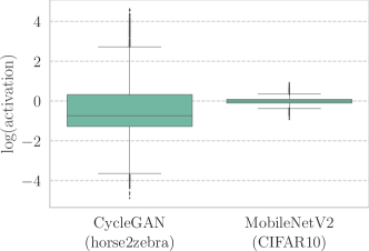
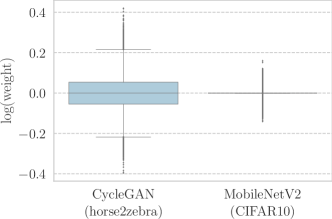
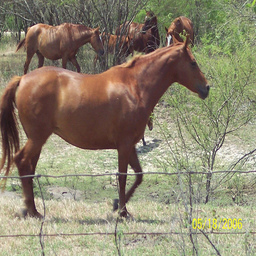
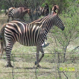
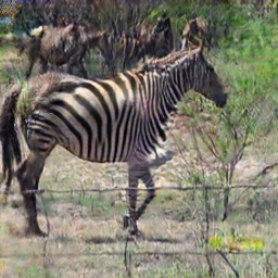
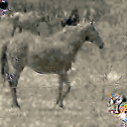
Saturated Quantization. Due to the adaptive nature of our delayed quantization operator, the estimation of the optimal decimal bits ($d^{*}$) as given by Eq. 3 can be sensitive to extreme outliers in the weight or activation distributions. In our experiments, we observe a long-tailed distribution only in the activation space of DNNs trained on generative tasks — more specifically, generative adversarial networks (GANs). As depicted in Fig. 3, the distribution of activations sampled from CycleGAN  (Zhu et al.,, 2017) trained on “horse2zebra" has a much wider range than that of MobileNetV2 trained on CIFAR10. These extreme outliers result in the underestimation of $d^{*}$ and lead to catastrophic degradation of image fidelity, as shown in Fig. 4.

Wang et al., (2019) observe a similar phenomenon in the weights space of GANs and attribute this reduction in network performance to the under-representation of quantized values. Unlike their solution, which is a GAN-specific quantization method based on the expectation-maximization (EM) algorithm, we discover that this under-representation issue can be simply and effectively moderated by clipping the outliers.

Before estimating the optimal decimal bits ($d^{*}$) using Eq. 3, we apply a data-driven saturation function $S_{q_{l},q_{u}}(\mathbf{x})$ defined by Eq. 5. Here, $\mathbf{x}$ denotes the input to the operator (e.g., activations), $q_{l}$ denotes the lower quantile of the distribution of sampled activations using Eq. 6, and $q_{u}$ similarly denotes the upper quantile. Note that $q_{l}$ and $q_{u}$ are hyperparameters such that $q_{l},q_{u}\in[0,1]$ and $q_{l}<q_{u}$. In our experiments with CycleGAN, we use quantiles $q_{l}=0.01\%$ and $q_{u}=99.99\%$.

$$S_{q_{l},q_{u}}(\mathbf{x})=\text{clip}(\mathbf{x},\small{\text{quantile}}(\mathbf{x},q_{l}),\small{\text{quantile}}(\mathbf{x},q_{u}))$$ (5)

$$\text{quantile}(\mathbf{x},a)=a\text{-th quantile of }\mathbf{x}$$ (6)

Thus, when using delayed quantization for GANs, we estimate the optimal decimal bits using Eq. 7. As shown in Fig. 4, applying saturated quantization to the activations of GANs preserves generative quality.

$$d^{*}=\arg\min_{d}\|Q_{u}(\mathbf{x}_{t_{q}},d)-S_{q_{l},q_{u}}(\mathbf{x}_{t_{q}})\|^{2}$$ (7)

(a)

(b)

(c)

(d)

Figure 4: These images were generated from CycleGAN trained on “horse2zebra" using (a) as the input. The baseline (b) shows the resulting translation at full precision, (c) shows the resulting translation when trained at 8-bit precision with saturated quantization over the activation space as well as 50% weight and activation pruning, and (d) shows the resulting translation without saturated quantization. Experiment settings and notations are further detailed in Section 4.

3.2 Unstructured Pruning Method

Magnitude-based unstructured weight pruning has been shown to yield impressive compression rates while maintaining network performance similar to their fully connected counterparts (Han et al.,, 2015; Zhu and Gupta,, 2017; Gale et al.,, 2019). To do so, this class of techniques use weight magnitude as a surrogate for importance when identifying redundant weights to remove from the computation graph. Zhu and Gupta, (2017) propose an unstructured pruning technique that maintains a binary mask for each set of weights and allows for the reactivation of pruned elements throughout training. In this work, we extend this technique to also prune the activations of deep neural networks (DNNs).

As shown in Eq. 8, we denote the unstructured pruning operator $P(\mathbf{x},s)$ as element-wise multiplication between $\mathbf{x}$ and $\mathbf{M}_{\mathbf{x},s}$, where $\mathbf{x}$ denotes the input to the operator (i.e., weights or activations), $s$ denotes the target sparsity as measured by the percentage of zero-valued elements, and $\mathbf{M}_{\mathbf{x},s}$ denotes its binary mask. Given that $(i,j)$ are the row and column indices, respectively, the binary mask $\mathbf{M}_{\mathbf{x},s}$ is calculated using Eq. 9 where the quantile operation is defined by Eq. 6.

$$P(\mathbf{x},s)=\mathbf{x}\circ\mathbf{M}_{\mathbf{x},s}$$ (8)

$$\begin{split}\mathbf{M}_{\mathbf{x},s}^{(i,j)}&=\begin{cases}1&|\mathbf{x}^{(i,j)}|\geq\text{quantile}(|\mathbf{x}|,s)\\ 0&\text{otherwise}\end{cases}\end{split}$$ (9)

As proposed by Zhu and Gupta, (2017), the sparsity level ($s$) is controlled and updated according to a sparsification schedule at time steps $t_{p}+i\Delta t_{p}$ such that $i\in\{1,2,..,,n\}$, where $t_{p}$, $\Delta t_{p}$, and $n$ are hyperparameters that represent the starting step, frequency, and total number of steps, respectively.

Figure 5: Here, we evaluate the effect of window size ($T$) on the resulting PSNR of the ESPCN super resolution network evaluated over Set5.

As an artifact of the commonly used rectified linear unit (ReLU), the activations of DNNs are inherently sparse (Glorot et al.,, 2011; Xu et al.,, 2015); however, this sparsity pattern is neither structured nor static. Contrary to the weights of DNNs, which are static during inference, the activations of DNNs are dynamically conditioned on the input to the network (Zhou et al.,, 2016). This dynamic sparsity pattern is difficult to exploit or optimize during inference. To account for this without sacrificing computational efficiency, we introduce a sliding window technique to stabilize unstructured activation pruning throughout training.

Let $\mathbf{h}_{t}$ denote the activations at time $t$ and $T$ denote the size of the sliding window. We extend the calculation of the binary mask to the activations of DNNs as given by Eq. 9 by evaluating the mask over a running sum within a sliding window of size $T$ as is shown in Eq. 10.

$$\mathbf{M}_{\mathbf{h}_{t},s}(i,j)=\begin{cases}1&\sum\limits_{n=0}^{T-1}|\mathbf{h}_{t-n}(i,j)|\geq\text{\scriptsize quantile}(\sum\limits_{n=0}^{T-1}|\mathbf{h}_{t-n}|,s)\\ 0&\text{otherwise}\end{cases}$$ (10)

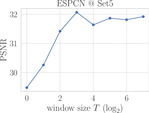
In Fig. 5, we evaluate the effect of window size ($T$) on the PNSR of a super resolution network (ESPCN) (Shi et al.,, 2016) on Set5 (Bevilacqua et al.,, 2012). We observe that while PSNR increases with $T$, the benefit of an increased window size saturates around 16. It is important to note that this not only indicates that our approach can estimate the expected activation pattern, it also aligns with the observation of Hanin and Rolnick, (2019) that ReLU-based DNNs express much fewer activation patterns than their theoretical limit. By applying unstructured pruning to the activation space of these DNNs, we exploit the severe under-utilization of a network’s potential expressiveness and significantly increase compression rates while maintaining performance.

4 Empirical Analysis

(a) Image Classification	Top-1 Acc	PD
Baseline	92.60	0.31
$P_{0.5}(w)\rightarrow Q_{8}(w,f)$	92.23	1.43
$Q_{8}(w,f)\rightarrow P_{0.5}(w)$	85.94	1.33

(b) Object Detection	mAP	PD
Baseline	74.47	0.33
$P_{0.5}(w)\rightarrow Q_{8}(w,f)$	74.44	0.71
$Q_{8}(w,f)\rightarrow P_{0.5}(w)$	74.13	0.71

(c) Super Resolution	PSNR	PD
Baseline	32.84	6.22
$P_{0.5}(w)\rightarrow Q_{8}(w,f)$	32.51	8.36
$Q_{8}(w,f)\rightarrow P_{0.5}(w)$	32.54	8.37

Table 3: Here, we empirically evaluate the non-commutativity hypothesis across both discriminative and generative computer vision tasks. While experiments (a) and (b) favor the standard “prune-the-quantize" training schedule, experiment (c) indicates the need to consider the alternative. Note that notations and experiment settings are discussed in Section 4.

(a) Image Classification	Top-1 Acc	PD
Baseline	92.60	0.31
$P_{0.5}(w,f)\rightarrow Q_{8}(w,f)$	91.44	2.49
$Q_{8}(w,f)\rightarrow P_{0.5}(w,f)$	86.84	2.36

(b) Object Detection	mAP	PD
Baseline	74.47	0.33
$P_{0.5}(w,f)\rightarrow Q_{8}(w,f)$	73.00	0.86
$Q_{8}(w,f)\rightarrow P_{0.5}(w,f)$	70.13	0.82

(c) Super Resolution	PSNR	PD
Baseline	32.84	6.22
$P_{0.5}(w,f)\rightarrow Q_{8}(w,f)$	31.03	8.34
$Q_{8}(w,f)\rightarrow P_{0.5}(w,f)$	31.66	8.51

Table 4: Here, we extend the experiments summarized in Table 3 to include the unstructured activation pruning techniques introduced in Section 3.2. Doing so further accentuates the exact ordering in which quantization and pruning should be introduced into the training schedule to optimize network performance.

In this section, we empirically evaluate the non-commutativity hypothesis and compare our framework to existing state-of-the-art solutions. We demonstrate that our methods deliver superior performance per memory footprint across the following discriminative and generative computer vision tasks:

1. Image classification with MobileNetV2 (Sandler et al.,, 2018) on CIFAR10 (Krizhevsky et al.,, 2009)

2. Object detection with Faster RCNN (Ren et al.,, 2015) using ResNet101 (He et al.,, 2016) on Pascal VOC (Everingham et al.,, 2010)

3. Super resolution with ESPCN (Shi et al.,, 2016) on Set5 (Bevilacqua et al.,, 2012)

4. Image-to-image translation with two generative adversarial networks (GANs): Pix2Pix (Isola et al.,, 2017) and CycleGAN (Zhu et al.,, 2017) trained on facades and horse2zebra, respectively

We implement each task using the existing open-source implementations as provided by their respective authors. We maintain their selected weight initialization techniques and apply all of the same hyperparameters aside from the number of training epochs. We provide further details on experiment setups in Appendix B.

As discussed in Section 3, our framework enables the consideration of both the “prune-then-quantize” and “quantize-then-prune” training schedules when applying our novel uniform quantization and unstructured pruning methods to both the weights and activations of DNNs. Given quantization delay $t_{q}$ and pruning delay $t_{p}$, we define $t_{+}=\text{max}(t_{p},t_{q})$ following Fig. 2. Note that this results in the “quantize-the-prune” paradigm when $t_{q}<t_{p}$ and “prune-then-quantize” otherwise.

We denote the “prune-then-quantize" training schedule as $P_{0.5}(w,f)\rightarrow Q_{8}(w,f)$ when applying both quantization and pruning to both the weights and activations of a DNN using 8-bit precision and a target sparsity of 50%. We denote its “quantize-then-prune" analog as $Q_{8}(w,f)\rightarrow P_{0.5}(w,f)$. Similarly, we denote the standard “prune-then-quantize" training schedule as $P_{0.5}(w)\rightarrow Q_{8}(w,f)$ for the case where no pruning is applied to the activations of the DNN.

Finally, we introduce a metric we refer to as performance density (PD), which we define as the domain-specific performance (e.g., accuracy, PSNR, mAP) divided by the resulting memory footprint of the combined weights and activations. Because increased levels of quantization and pruning invariably lead to drops in network performance, we use this metric to analyze the trade-off between compression and performance across both discriminative and generative tasks.

4.1 Non-Commutativity Hypothesis

To evaluate the non-commutativity hypothesis, we start by evaluating the currently accepted “prune-then-quantize" training schedule $P_{0.5}(w)\rightarrow Q_{8}(w,f)$ across experiments (a), (b), and (c). We compare this training schedule to its “quantize-then-prune" analog $Q_{8}(w,f)\rightarrow P_{0.5}(w)$ and provide the results in Table 3.

Our results indicate a need to rethink the commonly accepted “prune-then-quantize" paradigm. Whereas experiments (a) and (b) support the standard training schedule, experiment (c) highlights the benefits of considering the alternative. Our hypothesis is further strengthened when we apply our unstructured activation pruning methods detailed in Section 3.2.

As shown in Table 4, applying unstructured pruning to the activations in both training schedules further reinforces the correct order that optimizes performance density (PD). When comparing Tables 3 and 4, it is observed that the addition of activation pruning universally provides higher PD as the compression of the activation space significantly reduces the total memory footprint while maintaining network performance.

This result not only empirically validates that there exists an optimal order in which quantization and pruning should be introduced into the training schedule to optimize network performance, it also indicates that this ordering varies across discriminative and generative tasks. As shown in Table 5, this trend holds when extended to experiment (d)—GANs trained for image-to-image translation. The majority of existing works studying quantization and pruning techniques primarily focus on discriminative tasks (e.g., image classification) rather than generative tasks (e.g., image-to-image translation). Recent studies have shown impressive results when applying these techniques to GANs (Wang et al.,, 2019; Zhou et al.,, 2020). We extend our framework to Pix2Pix (d-1) and CycleGAN (d-2) and observe that both networks favor the “quantize-then-prune" training schedule.

(d-1) Pix2Pix	FID	PD
Baseline	119.9	3.67
$P_{0.5}(w,f)\rightarrow Q_{8}(w,f)$	154.8	22.37
$Q_{8}(w,f)\rightarrow P_{0.5}(w,f)$	135.0	25.66

(d-2) CycleGAN	FID	PD
Baseline	67.1	3.28
$P_{0.5}(w,f)\rightarrow Q_{12}(w,f)$	100.4	16.67
$Q_{12}(w,f)\rightarrow P_{0.5}(w,f)$	89.4	18.73

Table 5: Here, we extend the experiments summarized in Table 4 to GANs trained for image-to-image translation. To quantify generative quality, we use the inverse of the Fréchet Inception Distance (FID) (Heusel et al.,, 2017) between the generated samples and real images as the domain-specific performance metric used to calculate PD. Note that a lower FID indicates higher generative quality. In our experiments, we find the CycleGAN activations require a higher bitwidth to maintain network performance.

Method	Network	$N_{W}$	$N_{A}$	$s_{W}$	$s_{A}$	Baseline Acc	Accuracy	Weights (Mb)	Activations (Mb)	PD (Acc/Mb)
(Choi et al.,, 2016)	ResNet-32	8	–	77.8%	–	92.58	92.64 (+0.06)	37.80	131.07	0.55
(Achterhold et al.,, 2018)	DenseNet-76	2	–	54%	–	92.19	91.17 (-1.02)	0.68	282.53	0.32
(Liu et al.,, 2018)	VGG-19	–	–	80%	–	93.5	93.52 (+0.02)	128.26	38.80	0.56
	PreResNet-110	–	–	30%	–	95.04	95.06 (+0.02)	952.03	619.71	0.06
	DenseNet-100	–	–	30%	–	95.24	95.21 (-0.03)	27.11	426.74	0.21
(Zhao et al., 2019a, )	DenseNet-40	–	–	59.7%	–	94.11	93.16 (-0.95)	3.23	114.87	0.79
(Xiao and Wang,, 2019)	VGG-16	–	–	79%	–	93.40	91.5 (-1.9)	98.97	35.39	0.68
(Dettmers and Zettlemoyer,, 2019)	VGG16-C	–	–	95%	–	93.51	93 (-0.51)	23.57	35.39	1.58
	WRN-22-8	–	–	95%	–	95.74	95.07 (-0.67)	27.46	230.69	0.37
(Yang et al.,, 2020)	ResNet-20	1.9	–	54%	–	91.29	91.15 (-0.14)	9.77	78.64	1.03
(van Baalen et al.,, 2020)	VGG-7	4.8	5.4	–	–	93.05	93.23 (+0.18)	43.85	3.27	1.98
(Paupamah et al.,, 2020)	MobileNet	8	8	–	–	91.31	90.59 (-0.72)	25.74	13.17	2.33
(Choi et al.,, 2020)	ResNet-32	8	–	87.5%	–	92.58	92.57 (-0.01)	21.28	131.07	0.61
Ours	MobileNetV2	8	8	50%	–	92.60	92.23 (-0.37)	9.19	55.20	1.43
		8	8	50%	50%		91.44 (-1.16)	9.19	27.60	2.49

Table 6: We demonstrate the superior performance per memory footprint (i.e., performance density) of our framework when compared to existing image classification solutions trained on CIFAR10. By jointly applying uniform quantization and unstructured pruning to both the weights and activations of the DNN, we achieve a higher performance density (PD) with lower compression rates than existing solutions and comparable network performance.

4.2 Comparing Against Existing Methods

Using the optimal orderings determined in Section 4.1, we demonstrate that our framework achieves superior performance per memory footprint (i.e. performance density) when compared to existing image classification solutions trained on on CIFAR10. Table 6 summarizes this comparison, where $N_{W}$ and $N_{A}$ denote the average number of bits used to quantize the weights or activations, respectively. Similarly, $s_{W}$ and $s_{A}$ denote the average weight and activation sparsity, respectively.

From Table 6, it can be observed that our method is uniquely comprehensive, supporting both quantization and pruning over both the weights and activations. Furthermore, our framework achieves the smallest memory footprint and highest performance density (PD) when applying unstructured pruning to the activation space. Unlike methods such as (Yang et al.,, 2020; van Baalen et al.,, 2020), our framework provides direct control over the target bitwidth and sparsity, which is more useful in practical scenarios under tight design constraints.

5 Discussion

It has been shown that activations dominate data movement and therefore time and energy costs during inference in real-time computer vision applications (Horowitz,, 2014; Jha et al.,, 2021; Colbert et al.,, 2021). Extending unstructured pruning to the activation space not only significantly improves the network performance per memory footprint, it also reduces the cost of running inference in resource-constrained settings with limited compute and memory budgets such as edge or mobile computing.

The prevalence of deep learning solutions for edge and mobile applications has resulted in a trend of minimizing the compute and memory requirements of over-parameterized networks. However, since the performance of DNNs is known to scale with the size of the network (Hestness et al.,, 2017), using PD to compare existing solutions that apply quantization and pruning across various neural network architectures provides a holistic view of the compression-accuracy trade-off.

When analyzing our framework, Tables 4 and 5 show discriminative tasks favor the “prune-then-quantize” training schedule while generative tasks favor the alternative. Based on these results, we articulate the non-commutativity conjecture.

The Non-Commutativity Conjecture. The optimal schedule in which quantization and pruning are introduced throughout training is intimately tied to the magnitude of the network’s gradient updates.

Applying unstructured activation pruning throughout training invariably results in shifts in the distribution of activations, which are known to lead to exploding gradients (Littwin and Wolf,, 2018). However, applying STE-based quantization inherently constrains both the activation distribution and their resulting gradients using clipping as shown in Eq. 1 and 2. Additionally, it has been shown that batch normalization stablilizes the distribution of gradients (Santurkar et al.,, 2018). Whereas the authors of the selected discriminative tasks (a) and (b) both utilize batch normalization, the authors of the selected generative tasks (c) and (d) do not. Thus, we conjecture that for the selected generative tasks, quantization acts as a regularizer to stabilize the distribution shifts caused by unstructured activation pruning.

6 Conclusions and Future Work

We propose a framework to apply novel methods for uniform quantization and unstructured pruning to both the weights and activations of DNNs during training. To the best of our knowledge, we are the first to thoroughly evaluate the impact of applying unstructured activation pruning in this setting. Unlike previous work, our framework enables the consideration of both the standard “prune-then-quantize” training schedule as well as its “quantize-the-prune” analog. Using this framework, we evaluate the performance of our methods when jointly applied to DNNs trained over a wide range of discriminative and generative tasks. Based on our observations, we articulate and evaluate the non-commutativity hypothesis to determine that the optimal ordering in which quantization and pruning are introduced into the training schedule not only exists, but also varies across tasks. Using the optimal training schedules for each task, we demonstrate the superior performance per memory footprint of our framework when compared to existing solutions. In future work, we aim to extend our analyses to larger network architectures trained on more complex datasets for tasks not limited to computer vision. Additionally, we aim to explore the application of neural architecture search algorithms in automating the selection and design of layer-specific training schedules.

Appendix

Appendix A Software Library

The code for each algorithm introduced in this paper can be found in our Python library, qsparse, at https://github.com/mlzxy/qsparse. In Listing 6, we provide an example of how to use our algorithms for uniform quantization and unstructured pruning as PyTorch modules (Paszke et al.,, 2019).

The majority of existing model compression and quantization Python libraries provide a minimal set of specialized modules separated, which limits the flexibility of the software interface (Pappalardo,, 2021; Coelho Jr et al.,, 2020; Qat,, 2021). However, the simplicity of our framework enables an efficient software interface. In contrast, qsparse supports a wide range of neural network specifications. To improve the library flexibility, we introduce a technique which directly transforms the weight attribute of the input layer into a pruned or quantized version at runtime. Thus, our library is layer-agnostic and can work with any PyTorch module as long as their parameters can be accessed from their weight attribute, as is standard practice (Paszke et al.,, 2019).

import torch.nn as nnfrom qsparse import prune, quantize# feature pruning and quantizationnn.Sequential(nn.Conv2d(10, 30, 3),prune(0.5, start=1000, interval=100, repetition=3),quantize(bits=8, timeout=2000)  # ‘timeout‘ is ‘quantize step‘ in Alg. 1)# weight pruning and quantization (layers other than ‘Conv2d‘ work as well)qpconv = quantize(prune(nn.Conv2d(10, 30, 3), 0.5), 8)

Figure 6: Examples of our software interface for quantization and pruning on both weights and features

Appendix B Experiment Setup

Using our library, we introduce minimal code changes to the original open-source implementations used for our experiments. We will release the code of each experiment as examples for our library. For each experiment, we maintain the hyperparameters selected by the original authors aside from the number of training epochs. Table 7 summarizes the hyperparameters considered in our experiments.

Param	Description
$t_{q}$	The number of epochs to delay quantization
$q_{u}$	The upper quantile used for saturated quantization
$q_{l}$	The lower quantile used for saturated quantization
$t_{p}$	The number of epochs to delay unstructured pruning
$\Delta t_{p}$	The frequency of updates to the binary mask
$n$	The total number of pruning steps applied throughout training
$T$	The window size used for unstructured activation pruning
$E$	The total number of training epochs

Table 7: Summary of the hyperparameters considered in this work

B.1 Image Classification on Cifar10

We use (kua,, 2021) as the foundation of our image classification experiments and train MobileNetV2 (Sandler et al.,, 2018) on CIFAR10 (Krizhevsky et al.,, 2009). We quantize all the weights and activations to 8-bit precision and use a target sparsity of 50%. We do not quantize the bias as it is typically stored and computed at full precision during on-device inference (Jacob et al.,, 2018). We apply unstructured pruning to both the weights and activations of all hidden layers, leaving the first and last layers densely connected. We set the total number of training epochs ($E$) to 250, $q_{u}$ to 0, $q_{l}$ to 1, and $T$ to $2048$ in each experiment.

Experiment	Settings
$P_{0.5}(*)\rightarrow Q_{8}(*)$	$t_{q}$ was set to 230 and 235 for the weights and activations, respectively. $t_{p},\Delta t_{p},\text{ and }n$ were set to $100,15,\text{ and }4$, respectively.
$Q_{8}(*)\rightarrow P_{0.5}(*)$	$t_{q}$ was set to 160 and 170 for the weights and activations, respectively. $t_{p},\Delta t_{p},\text{ and }n$ were set to 180,15, and 4, respectively.
$Q_{8}(*)$	$t_{q}$ was set to 230 and 240 for the weights and activations, respectively.

Table 8: Summary of the hyperparameters used for image classification

We calculate the performance density (PD) for this task as the accuracy divided by the combined size of the weights and activation of the network in megabits (Mb), such that the units are accuracy-per-megabit (Acc/Mb). The memory footprint of the activations is calculated assuming an input size of (3, 32, 32).

B.2 Super Resolution on Set5

We use (yjn,, 2019) as the foundation of our super resolution experiments and train ESPCN (Shi et al.,, 2016) for using 91-image (Yang et al.,, 2010). Similar to the experiments outlined in Appendix B.1, we quantize all weights and activations at 8-bit precision using a target sparsity of 50% without pruning for first and last layer of the network. We set $E$ to 200, $q_{u}$ to 0, $q_{l}$ to 1, and $T$ to $16$ in each experiment.

Experiment	Settings
$P_{0.5}(*)\rightarrow Q_{8}(*)$	$t_{q}$ was set to 160 and 170 for the weights and activations, respectively. $t_{p},\Delta t_{p},\text{ and }n$ were set to $140,5,\text{ and }4$, respectively.
$Q_{8}(*)\rightarrow P_{0.5}(*)$	$t_{q}$ was set to 140 and 150 for the weights and activations, respectively. $t_{p},\Delta t_{p},\text{ and }n$ were set to 155,5, and 4, respectively.
$Q_{8}(*)$	$t_{q}$ was set to 140 and 150 for the weights and activations, respectively.

Table 9: Summary of the hyperparameters used for super resolution

ESPCN is a fully convolutional network which is trained to upsample image patches of size (17, 17) to (48, 48). During testing, ESPCN is used to upsample images of size (170, 170) to (480, 480). Due to the unequal sizes of training and testing images, the binary mask $\mathbf{M}_{\mathbf{x},s}$ resulting from training using unstructured activation pruning cannot be directly applied for testing. Accounting for this mismatch, we replicate the binary mask $\mathbf{M}_{\mathbf{x},s}$ along the height and width axis of each feature map to align with the testing size requirements.

We calculate the performance density (PD) for this task as the peak signal-to-noise ratio (PSNR) divided by the log of the combined size of the weights and activations as measure in megabits (Mb) such that the units are PSNR / log(Mb). We use $\log$ here as PSNR is a logarithmic domain metric. The memory footprint of the activations is calculated assuming an input size of (1, 170, 170).

B.3 Objection Detection on Pascal VOC

We use (Yang et al.,, 2017) as the foundation of our object detection experiments and train Faster RCNN (Ren et al.,, 2015) using ResNet101 (He et al.,, 2016) on the Pascal VOC dataset (Everingham et al.,, 2010) for all experiments. ResNet101 is pretrained on ImageNet dataset (Russakovsky et al.,, 2015). We follow a experiment setup similar to Appendix B.1, but we do not quantize or prune the first 3 residual blocks as they are frozen in the original paper (Ren et al.,, 2015). We also freeze all pre-trained batch normalization layers. However, these limitations can be overcome with group normalization or synchronized batch normalization according to He et al., (2019). We set $E$ to 9, $q_{u}$ to 0, $q_{l}$ to 1, and $T$ to $32$ in each experiment.

Experiment	Settings
$P_{0.5}(*)\rightarrow Q_{8}(*)$	$t_{q}$ was set to 7.2 and 7.5 for the weights and activations, respectively. $t_{p},\Delta t_{p},\text{ and }n$ were set to $3,0.5,\text{ and }4$, respectively.
$Q_{8}(*)\rightarrow P_{0.5}(*)$	$t_{q}$ was set to 5.2 and 5.5 for the weights and activations, respectively. $t_{p},\Delta t_{p},\text{ and }n$ were set to 5.7, 0.5, and 4, respectively.
$Q_{8}(*)$	$t_{q}$ was set to 5.2 and 5.5 for the weights and activations, respectively.

Table 10: Summary of the hyperparameters used for object detection

Since the image sizes differ between each batch during training, we cannot obtain a fixed size binary mask $\mathbf{M}_{\mathbf{x},s}$ on activation of the convolution layers. Alternatively, we apply channel-wise pruning on convolution activations.

We calculate the performance density (PD) for this task as mean average precision (mAP) divided by the combined size of the weights and activations as measure in gigabits (Gb), such that the units are mAP/Gb. The memory footprint of the activations is calculated assuming an input size of (3, 480, 720).

B.4 Pix2Pix on Facades and CycleGAN on Horse2zebra

We use Pix2Pix (Isola et al.,, 2017) and CycleGAN (Zhu et al.,, 2017) in our generative adversarial network (GAN) experiments. While Pix2Pix uses a UNet architecture (Ronneberger et al.,, 2015), CycleGAN uses a variant of ResNet with deconvolution layers. We use an experimental setup similar to Appendix B.1, but we use 12-bit quantization over the activations of CycleGAN. In addition to skipping first and last layer, we also skip both the second and second-to-last layer of CycleGAN as well as the inner-most UNet layer of Pix2Pix. We set $q_{u}$ to 0 and $q_{l}$ to 1 in each Pix2Pix experiment and $q_{u}$ to 0.0001 and $q_{l}$ to 0.9999 in each CycleGAN experiment. All other hyperparameters are the same between Pix2Pix and CycleGAN. We set $E$ to $300$ and $T$ to $128$.

Experiment	Settings
$P_{0.5}(*)\rightarrow Q_{8}(*)$	$t_{q}$ was set to 280 and 290 for the weights and activations, respectively. $t_{p},\Delta t_{p},\text{ and }n$ were set to $100,15,\text{ and }4$, respectively.
$Q_{8}(*)\rightarrow P_{0.5}(*)$	$t_{q}$ was set to 110 and 120 for the weights and activations, respectively. $t_{p},\Delta t_{p},\text{ and }n$ were set to 130, 15, and 4, respectively.
$Q_{8}(*)$	$t_{q}$ was set to 110 and 120 for the weights and activations, respectively.

Table 11: Summary of the hyperparameters used for object detection

We calculate the performance density (PD) for each task as the Fréchet Inception Distance (FID) divided by the combined size of the weights and activations as measured in bits such that the units are 1/(FID*bits). The memory footprint of the activations is calculated assuming an input size of (3, 256, 256). Figures 7 and 8 respectively show examples of images generated from Pix2Pix and CycleGAN.

Figure 7: Examples of generated images from Pix2Pix.

Figure 8: Examples of generated images from CycleGAN.

References

- yjn, (2019) (2019). yjn870/espcn-pytorch: Pytorch implementation of real-time single image and video super-resolution using an efficient sub-pixel convolutional neural network (cvpr 2016). https://github.com/yjn870/ESPCN-pytorch. (Accessed on 10/05/2021).
- kua, (2021) (2021). kuangliu/pytorch-cifar: 95.47% on cifar10 with pytorch. https://github.com/kuangliu/pytorch-cifar. (Accessed on 10/05/2021).
- Qat, (2021) (2021). torch.nn.qat — pytorch 1.9.0 documentation. https://pytorch.org/docs/stable/torch.nn.qat.html. (Accessed on 09/01/2021).
- Achterhold et al., (2018) Achterhold, J., Koehler, J. M., Schmeink, A., and Genewein, T. (2018). Variational network quantization. In International Conference on Learning Representations.
- Bevilacqua et al., (2012) Bevilacqua, M., Roumy, A., Guillemot, C., and Alberi-Morel, M. L. (2012). Low-complexity single-image super-resolution based on nonnegative neighbor embedding.
- Bhalgat et al., (2020) Bhalgat, Y., Lee, J., Nagel, M., Blankevoort, T., and Kwak, N. (2020). LSQ+: improving low-bit quantization through learnable offsets and better initialization. CoRR, abs/2004.09576.
- Choi et al., (2016) Choi, Y., El-Khamy, M., and Lee, J. (2016). Towards the limit of network quantization. arXiv preprint arXiv:1612.01543.
- Choi et al., (2020) Choi, Y., El-Khamy, M., and Lee, J. (2020). Universal deep neural network compression. IEEE Journal of Selected Topics in Signal Processing, 14(4):715–726.
- Coelho Jr et al., (2020) Coelho Jr, C. N., Kuusela, A., Zhuang, H., Aarrestad, T., Loncar, V., Ngadiuba, J., Pierini, M., and Summers, S. (2020). Ultra low-latency, low-area inference accelerators using heterogeneous deep quantization with qkeras and hls4ml. arXiv e-prints, pages arXiv–2006.
- Colbert et al., (2021) Colbert, I., Kreutz-Delgado, K., and Das, S. (2021). An energy-efficient edge computing paradigm for convolution-based image upsampling. arXiv preprint arXiv:2107.07647.
- Dettmers and Zettlemoyer, (2019) Dettmers, T. and Zettlemoyer, L. (2019). Sparse networks from scratch: Faster training without losing performance. arXiv preprint arXiv:1907.04840.
- Everingham et al., (2010) Everingham, M., Van Gool, L., Williams, C. K., Winn, J., and Zisserman, A. (2010). The pascal visual object classes (voc) challenge. International journal of computer vision, 88(2):303–338.
- Frankle and Carbin, (2018) Frankle, J. and Carbin, M. (2018). The lottery ticket hypothesis: Finding sparse, trainable neural networks. arXiv preprint arXiv:1803.03635.
- Gale et al., (2019) Gale, T., Elsen, E., and Hooker, S. (2019). The state of sparsity in deep neural networks. arXiv preprint arXiv:1902.09574.
- Gholami et al., (2021) Gholami, A., Kim, S., Dong, Z., Yao, Z., Mahoney, M. W., and Keutzer, K. (2021). A survey of quantization methods for efficient neural network inference. arXiv preprint arXiv:2103.13630.
- Glorot and Bengio, (2010) Glorot, X. and Bengio, Y. (2010). Understanding the difficulty of training deep feedforward neural networks. In Proceedings of the thirteenth international conference on artificial intelligence and statistics, pages 249–256. JMLR Workshop and Conference Proceedings.
- Glorot et al., (2011) Glorot, X., Bordes, A., and Bengio, Y. (2011). Deep sparse rectifier neural networks. In Proceedings of the fourteenth international conference on artificial intelligence and statistics, pages 315–323. JMLR Workshop and Conference Proceedings.
- Gray et al., (2017) Gray, S., Radford, A., and Kingma, D. P. (2017). Gpu kernels for block-sparse weights. arXiv preprint arXiv:1711.09224, 3.
- Han et al., (2015) Han, S., Mao, H., and Dally, W. J. (2015). Deep compression: Compressing deep neural networks with pruning, trained quantization and huffman coding. arXiv preprint arXiv:1510.00149.
- Hanin and Rolnick, (2019) Hanin, B. and Rolnick, D. (2019). Deep relu networks have surprisingly few activation patterns.
- He et al., (2019) He, K., Girshick, R., and Dollár, P. (2019). Rethinking imagenet pre-training. In Proceedings of the IEEE/CVF International Conference on Computer Vision, pages 4918–4927.
- He et al., (2016) He, K., Zhang, X., Ren, S., and Sun, J. (2016). Deep residual learning for image recognition. In Proceedings of the IEEE conference on computer vision and pattern recognition, pages 770–778.
- Hestness et al., (2017) Hestness, J., Narang, S., Ardalani, N., Diamos, G., Jun, H., Kianinejad, H., Patwary, M., Ali, M., Yang, Y., and Zhou, Y. (2017). Deep learning scaling is predictable, empirically. arXiv preprint arXiv:1712.00409.
- Heusel et al., (2017) Heusel, M., Ramsauer, H., Unterthiner, T., Nessler, B., and Hochreiter, S. (2017). Gans trained by a two time-scale update rule converge to a local nash equilibrium. Advances in neural information processing systems, 30.
- Hinton et al., (2012) Hinton, G., Srivastava, N., and Swersky, K. (2012). Neural networks for machine learning. Coursera, video lectures, 264(1):2146–2153.
- Hoefler et al., (2021) Hoefler, T., Alistarh, D., Ben-Nun, T., Dryden, N., and Peste, A. (2021). Sparsity in deep learning: Pruning and growth for efficient inference and training in neural networks. arXiv preprint arXiv:2102.00554.
- Horowitz, (2014) Horowitz, M. (2014). 1.1 computing’s energy problem (and what we can do about it). In 2014 IEEE International Solid-State Circuits Conference Digest of Technical Papers (ISSCC), pages 10–14. IEEE.
- Hu et al., (2016) Hu, H., Peng, R., Tai, Y.-W., and Tang, C.-K. (2016). Network trimming: A data-driven neuron pruning approach towards efficient deep architectures. arXiv preprint arXiv:1607.03250.
- Hubara et al., (2017) Hubara, I., Courbariaux, M., Soudry, D., El-Yaniv, R., and Bengio, Y. (2017). Quantized neural networks: Training neural networks with low precision weights and activations. The Journal of Machine Learning Research, 18(1):6869–6898.
- Isola et al., (2017) Isola, P., Zhu, J.-Y., Zhou, T., and Efros, A. A. (2017). Image-to-image translation with conditional adversarial networks. In Proceedings of the IEEE conference on computer vision and pattern recognition, pages 1125–1134.
- Jacob et al., (2018) Jacob, B., Kligys, S., Chen, B., Zhu, M., Tang, M., Howard, A., Adam, H., and Kalenichenko, D. (2018). Quantization and training of neural networks for efficient integer-arithmetic-only inference. In Proceedings of the IEEE conference on computer vision and pattern recognition, pages 2704–2713.
- Jha et al., (2021) Jha, N. K., Mittal, S., and Avancha, S. (2021). Data-type aware arithmetic intensity for deep neural networks. Energy, 120:x109.
- Krishnamoorthi, (2018) Krishnamoorthi, R. (2018). Quantizing deep convolutional networks for efficient inference: A whitepaper. arXiv preprint arXiv:1806.08342.
- Krizhevsky et al., (2009) Krizhevsky, A., Hinton, G., et al. (2009). Learning multiple layers of features from tiny images.
- Liang et al., (2021) Liang, T., Glossner, J., Wang, L., Shi, S., and Zhang, X. (2021). Pruning and quantization for deep neural network acceleration: A survey. Neurocomputing, 461:370–403.
- Littwin and Wolf, (2018) Littwin, E. and Wolf, L. (2018). Regularizing by the variance of the activations’ sample-variances. arXiv preprint arXiv:1811.08764.
- Liu et al., (2018) Liu, Z., Sun, M., Zhou, T., Huang, G., and Darrell, T. (2018). Rethinking the value of network pruning. arXiv preprint arXiv:1810.05270.
- Pappalardo, (2021) Pappalardo, A. (2021). Xilinx/brevitas. https://doi.org/10.5281/zenodo.3333552.
- Paszke et al., (2019) Paszke, A., Gross, S., Massa, F., Lerer, A., Bradbury, J., Chanan, G., Killeen, T., Lin, Z., Gimelshein, N., Antiga, L., et al. (2019). Pytorch: An imperative style, high-performance deep learning library. Advances in neural information processing systems, 32:8026–8037.
- Paupamah et al., (2020) Paupamah, K., James, S., and Klein, R. (2020). Quantisation and pruning for neural network compression and regularisation. In 2020 International SAUPEC/RobMech/PRASA Conference, pages 1–6. IEEE.
- Ren et al., (2015) Ren, S., He, K., Girshick, R., and Sun, J. (2015). Faster r-cnn: Towards real-time object detection with region proposal networks. Advances in neural information processing systems, 28:91–99.
- Ronneberger et al., (2015) Ronneberger, O., Fischer, P., and Brox, T. (2015). U-net: Convolutional networks for biomedical image segmentation. In International Conference on Medical image computing and computer-assisted intervention, pages 234–241. Springer.
- Russakovsky et al., (2015) Russakovsky, O., Deng, J., Su, H., Krause, J., Satheesh, S., Ma, S., Huang, Z., Karpathy, A., Khosla, A., Bernstein, M., Berg, A. C., and Fei-Fei, L. (2015). ImageNet Large Scale Visual Recognition Challenge. International Journal of Computer Vision (IJCV), 115(3):211–252.
- Sandler et al., (2018) Sandler, M., Howard, A., Zhu, M., Zhmoginov, A., and Chen, L.-C. (2018). Mobilenetv2: Inverted residuals and linear bottlenecks. In Proceedings of the IEEE conference on computer vision and pattern recognition, pages 4510–4520.
- Santurkar et al., (2018) Santurkar, S., Tsipras, D., Ilyas, A., and Mądry, A. (2018). How does batch normalization help optimization? In Proceedings of the 32nd international conference on neural information processing systems, pages 2488–2498.
- Shi et al., (2016) Shi, W., Caballero, J., Huszár, F., Totz, J., Aitken, A. P., Bishop, R., Rueckert, D., and Wang, Z. (2016). Real-time single image and video super-resolution using an efficient sub-pixel convolutional neural network. In Proceedings of the IEEE conference on computer vision and pattern recognition, pages 1874–1883.
- van Baalen et al., (2020) van Baalen, M., Louizos, C., Nagel, M., Amjad, R. A., Wang, Y., Blankevoort, T., and Welling, M. (2020). Bayesian bits: Unifying quantization and pruning. arXiv preprint arXiv:2005.07093.
- Wang et al., (2019) Wang, P., Wang, D., Ji, Y., Xie, X., Song, H., Liu, X., Lyu, Y., and Xie, Y. (2019). Qgan: Quantized generative adversarial networks. arXiv preprint arXiv:1901.08263.
- Wang and Zhu, (2020) Wang, W. and Zhu, L. (2020). Structured feature sparsity training for convolutional neural network compression. Journal of Visual Communication and Image Representation, 71:102867.
- Wu et al., (2020) Wu, H., Judd, P., Zhang, X., Isaev, M., and Micikevicius, P. (2020). Integer quantization for deep learning inference: Principles and empirical evaluation. arXiv preprint arXiv:2004.09602.
- Xiao and Wang, (2019) Xiao, X. and Wang, Z. (2019). Autoprune: Automatic network pruning by regularizing auxiliary parameters. Advances in Neural Information Processing Systems 32 (NeurIPS 2019), 32.
- Xu et al., (2015) Xu, B., Wang, N., Chen, T., and Li, M. (2015). Empirical evaluation of rectified activations in convolutional network. arXiv preprint arXiv:1505.00853.
- Yang et al., (2020) Yang, H., Gui, S., Zhu, Y., and Liu, J. (2020). Automatic neural network compression by sparsity-quantization joint learning: A constrained optimization-based approach. In Proceedings of the IEEE/CVF Conference on Computer Vision and Pattern Recognition, pages 2178–2188.
- Yang et al., (2017) Yang, J., Lu, J., Batra, D., and Parikh, D. (2017). A faster pytorch implementation of faster r-cnn. https://github.com/jwyang/faster-rcnn.pytorch.
- Yang et al., (2010) Yang, J., Wright, J., Huang, T. S., and Ma, Y. (2010). Image super-resolution via sparse representation. IEEE transactions on image processing, 19(11):2861–2873.
- Yin et al., (2019) Yin, P., Lyu, J., Zhang, S., Osher, S., Qi, Y., and Xin, J. (2019). Understanding straight-through estimator in training activation quantized neural nets. arXiv preprint arXiv:1903.05662.
- Yu et al., (2020) Yu, P.-H., Wu, S.-S., Klopp, J. P., Chen, L.-G., and Chien, S.-Y. (2020). Joint pruning & quantization for extremely sparse neural networks. arXiv preprint arXiv:2010.01892.
- (58) Zhao, C., Ni, B., Zhang, J., Zhao, Q., Zhang, W., and Tian, Q. (2019a). Variational convolutional neural network pruning. In Proceedings of the IEEE/CVF Conference on Computer Vision and Pattern Recognition, pages 2780–2789.
- (59) Zhao, Y., Gao, X., Bates, D., Mullins, R., and Xu, C.-Z. (2019b). Focused quantization for sparse cnns. Advances in Neural Information Processing Systems, 32:5584–5593.
- Zhou et al., (2016) Zhou, B., Khosla, A., A., L., Oliva, A., and Torralba, A. (2016). Learning Deep Features for Discriminative Localization. CVPR.
- Zhou et al., (2020) Zhou, K., Gao, S., Cheng, J., Gu, Z., Fu, H., Tu, Z., Yang, J., Zhao, Y., and Liu, J. (2020). Sparse-gan: Sparsity-constrained generative adversarial network for anomaly detection in retinal oct image. In 2020 IEEE 17th International Symposium on Biomedical Imaging (ISBI), pages 1227–1231. IEEE.
- Zhu et al., (2017) Zhu, J.-Y., Park, T., Isola, P., and Efros, A. A. (2017). Unpaired image-to-image translation using cycle-consistent adversarial networks. In Proceedings of the IEEE international conference on computer vision, pages 2223–2232.
- Zhu and Gupta, (2017) Zhu, M. and Gupta, S. (2017). To prune, or not to prune: exploring the efficacy of pruning for model compression. arXiv preprint arXiv:1710.01878.