NoiER: An Approach for Training more Reliable Fine-Tuned Downstream Task Models

Abstract

The recent development in pretrained language models trained in a self-supervised fashion, such as BERT, is driving rapid progress in the field of NLP. However, their brilliant performance is based on leveraging syntactic artifacts of the training data rather than fully understanding the intrinsic meaning of language. The excessive exploitation of spurious artifacts causes a problematic issue: The distribution collapse problem, which is the phenomenon that the model fine-tuned on downstream tasks is unable to distinguish out-of-distribution (OOD) sentences while producing a high confidence score. In this paper, we argue that distribution collapse is a prevalent issue in pretrained language models and propose noise entropy regularisation (NoiER) as an efficient learning paradigm that solves the problem without auxiliary models and additional data. The proposed approach improved traditional OOD detection evaluation metrics by 55% on average compared to the original fine-tuned models.

1 Introduction

Contextualised representations of pretrained language models (PLMs) like ELMo Peters et al. (2018), BERT Devlin et al. (2018), and GPT Radford et al. (2018) have accomplished promising results in many NLP tasks. LMs are fine-tuned on downstream tasks while achieving state-of-the-art (SOTA) performance, even exceeding that of humans in several datasets Rajpurkar et al. (2016); Zellers et al. (2018). This new paradigm has become a predominant framework that paves the way for immense progress in NLP. Many novel approaches have been proposed to obtain more elaborate contextualised representations Yang et al. (2019); Clark et al. (2020) or to reduce the size of the model while maintaining its performance Sanh et al. (2019). Based on the promising results of pre-trained LMs, numerous studies argue that they are capable of understanding human language Devlin et al. (2018); Ohsugi et al. (2019).

However, recent studies reveal that the performance of PLMs does not arise from human-level language understanding but is based on their ability to excessively leverage syntactic patterns of training data. Niven and Kao (2019) claim that BERT’s performance is entirely based on the exploitation of spurious statistical cues that are present in the training set. They modified the English Argument Reasoning Comprehension dataset Habernal et al. (2018) by adding adversarial examples that just one token of the original was negated. BERT’s performance on the modified dataset falls short of expectations as a consequence of the excessive usage of the cues in the original training set. Similarly, McCoy et al. (2019) figure out that BERT is only highly competent in leveraging syntactic heuristics. Experiments on the novel HANS dataset, which McCoy et al. (2019) designed to frustrate the heuristics, exhibits a significant decrease in BERT’s performance. Bender and Koller (2020) argue that the widespread belief that pre-trained LMs understand or comprehend is a hype. Based on the result of carefully designed thought experiments, Bender and Koller (2020) show that it is impossible to learn the meaning of language by only leveraging the form of sentences.

The model that lacks generalisation ability tend to fail on data from a different distribution, providing high-confidence predictions while being incorrect Goodfellow et al. (2015); Amodei et al. (2016); Hendrycks and Gimpel (2017). Therefore, the results of the above studies cast the following question:

Can PLMs distinguish in-distribution (IND) and out-of-distribution (OOD) sentences when fine-tuned on downstream tasks?

In the open real world, there exist a huge number of OOD instances. Therefore, even though the models perform brilliantly on a closed-distribution dataset, there is a low chance for the models to be employed in practice, provided that they are incapable of rejecting OOD sentences. Generating incorrect results on these inputs and conducting unwanted commands may result in disasters, which undermines the reliability and reputation of a model. It could also trigger even more severe outcomes, particularly in risk-sensitive applications. Hence, to insist that a model is intelligent and can truly understand language, it should at least be capable of rejecting OOD sentences, just as humans do.

In this paper, we empirically show that distribution collapse, the phenomenon that a model yields high confidence scores on OOD instances and fails to distinguish them from IND instances, is a prevalent issue in the pretraining and fine-tuning framework, even for a simple text classification task. Next, we propose a simple but effective approach, called noise entropy regularisation (NoiER), which has the ability to reject OOD sentences while maintaining a high classification performance. We experimentally confirm that our proposed approach not only alleviates distribution collapse but also outperforms baseline models devised for detecting OOD sentences. The main contributions of this paper can be briefly summarised as follows:

• Through experiments, we reveal that large pre-trained LMs suffer from the distribution collapse issue when fine-tuned on downstream tasks.

• We propose noise entropy regularisation (NoiER) as an efficient method that alleviates the distribution collapse problem without leveraging additional data or adding auxiliary models.

• Compared to the fine-tuned models, our approach produces better AUROC and EER, which are increased by 60% and 49%, respectively, while maintaining a high classification capacity.

2 Related Works

OOD detection plays a crucial role in industrial processes for ensuring reliability and safety Harrou et al. (2016). As a result, numerous studies have been made in various fields, including NLP.

Classification. A simple way to classify OOD instances is to add the “OOD” class to a classifier Kim and Kim (2018). However, this approach is practically inefficient, considering the enormously broad distribution of OOD data. Another approach is detecting OOD sentences in an unsupervised manner by using IND samples only, which is known under several different names, such as one-class classification or novelty detection. Some works that leverage distance-based Oh et al. (2018); Xu et al. (2019) or density-based Song and Suh (2019); Seo et al. (2020) methods have been proposed for text OOD detection. However, most of these approaches are computationally expensive for both training and inference, which interrupts their usage in practical applications.

GAN-based approach. Ryu et al. (2018) leveraged a generative adversarial network (GAN) for OOD sentence detection. They expected the discriminator to reject OOD sentences by training it to distinguish IND sentences from fake instances generated by the generator. Ryu et al. (2018) used pretrained sentence representations for training the GAN.

Threshold-based approach. This approach composes an OOD detector $g(x)$ that judges an instance is OOD if the criterion score is lower than a threshold, i.e., $g(x)=\mathbbm{1}\,(S(x)>\alpha)$, where $\alpha$ denotes a threshold, and $S(x)$ refers to the predicted criterion score. Hendrycks and Gimpel (2017) leveraged the maximum softmax probability (MSP) as the criterion. Ryu et al. (2017) trained a text classifier and an autoencoder, and used the reconstruction errors for discerning OOD sentences.

Liang et al. (2018) proposed a method, called ODIN, which improved the MSP-based approach Hendrycks and Gimpel (2017) by applying temperature scaling and input perturbations. Temperature scaling modifies the softmax output as follows:

$$\begin{gathered}S_{i}(\textrm{x};T)=\frac{exp(f_{i}(\textrm{x})/T)}{\sum_{i=1}^{N}exp(f_{i}(\textrm{x})/T)},\end{gathered}$$ (1)

where $T\in\mathbb{R}^{+}$ denotes the temperature scaling parameter and is set to 1 during training. Next, during the inference process, a small perturbation is added to the input as follows:

$$\begin{gathered}\tilde{\textrm{x}}=\textrm{x}-\epsilon sign(-\nabla_{x}log(S_{\hat{y}}(\textrm{x};T))),\end{gathered}$$ (2)

where $\epsilon$ is the perturbation magnitude and $S_{\hat{y}}(\textrm{x};T)$ $=$ $\max_{i}S_{i}(\textrm{x};T)$. Although ODIN is designed for image classification, it is applicable to any type of classification models. This method has a practical benefit in that model training is unnecessary.

Entropy regularisation. The entropy regularisation is designed to make a threshold-based approach better detect OOD. The model is trained to minimise both cross-entropy loss ($\mathcal{L}_{ce}$) and entropy regularisation loss ($\mathcal{L}_{er}$) that maximises the entropy of the predictive distribution for OOD instances, while making it closer to the uniform distribution. This leads the model to conduct correct predictions for IND samples, while being less confident on OOD instances, and hence improves the performance of the predictive distribution threshold-based methods.

In computer vision, Lee et al. (2018) trained a GAN-based OOD generator to produce OOD examples and used them for minimising $\mathcal{L}_{er}$. Hendrycks et al. (2019) leveraged out-of-distribution datasets to maximise the entropy. Zheng et al. (2020) proposed a model called ER-POG to detect OOD in dialog systems. They observed that generating OOD samples in the continuous space Ryu et al. (2018); Lee et al. (2018) is inefficient for text data. Instead, they leveraged an LSTM-based sequence-to-sequence (Seq2Seq) autoencoder and GAN to generate discrete token OOD samples.

3 Distribution Collapse

In this section, we delve into the distribution collapse issue of PLMs. We experimentally verify that the distribution collapse truly exists in PLMs when they are fine-tuned on downstream tasks.

3.1 IND and OOD Disparity

Assume that a text classification model $M$ is trained to classify a category $C_{i}\in\{C_{1},\ldots,C_{K}\}$ that belongs to IND.The model can detect OOD by rejecting examples that generate threshold-below MSP scores Hendrycks and Gimpel (2017). Therefore, it should produce a high MSP score for an IND instance to not reject it. On the contrary, the predictive distribution for an OOD instance should be close to the uniform distribution, i.e., zero confidence Lee et al. (2018); Hendrycks et al. (2019); Zheng et al. (2020). Therefore, we first define a uniform disparity (UD) for a given sentence set $S$ as follows:

$$\begin{gathered}UD(S,M)=\frac{1}{|S|}\sum_{s_{i}\in S}JSD(M(s_{i}),u),\end{gathered}$$ (3)

where $u$ refers to the uniform distribution, and $JSD$ denotes the Jensen-Shannon divergence. Next, for a given IND set $I$ and OOD set $O$, the IND-OOD disparity (IOD) is calculated as follows:

$$\begin{gathered}\!\!\!\!IOD(I,O,M)=UD(I,M)-UD(O,M).\end{gathered}$$ (4)

Note that the metric is higher the better. Also, it can generate a negative value, which is the most undesirable case.

Table 1: Statistics of datasets for the distribution collapse experiment

	AG’s News	Fake News	Corona Tweets
# of classes	4	2	5
Training set size	120,000	40,408	41,157
Test set size	7,600	4,490	3,798
Avg sentence length	9.61 tokens	17.02 tokens	41.85 tokens

3.2 Experiments

Datasets. For the experiments, we collected three datasets from different domains and tasks: AG’s News dataset Zhang et al. (2015) for topic classification, the Fake News classification dataset Ahmed et al. (2017), and the Corona Tweets dataset, which is designed to classify the sentiment of tweets regarding COVID 19. For AG’s News and Fake News data, we used article titles as input text. We only conducteded minor preprocessing, such as removing the URL and special symbols for a hashtag. The statistics of each dataset are presented in Table 1.

Table 2: Results for the verification of distribution collapse. The name of the dataset corresponds to the IND data. We trained each model 10 times and recorded the average of each metric. The notation “$\uparrow$” denotes that higher values are better, and “$\downarrow$” stands for lower values are better. For the IOD value, we multiplied the original figure with 100 unify the scale with the other metrics. The best values are formatted in bold. The figures of fine-tuned models show a significant difference compared to TFIDF-NB with $p$-value $<$ 0.05 ($\dagger$) and $p$-value $<$ 0.01 (*) using the t-test.

Model

AG’s News

Fake News

Corona Tweets

F1$\uparrow$

IOD$\uparrow$

AUROC$\uparrow$

EER$\downarrow$

F1$\uparrow$

IOD$\uparrow$

AUROC$\uparrow$

EER$\downarrow$

F1$\uparrow$

IOD$\uparrow$

AUROC$\uparrow$

EER$\downarrow$

BERT

89.40*

7.25*

75.87*

31.20*

98.55*

0.64$\dagger$

58.06

44.89

83.17*

-2.13*

40.65*

57.51*

DistilBERT

89.82*

7.35*

76.96*

30.48*

98.62*

1.48

59.94$\dagger$

44.64

81.61*

-2.24*

41.63*

57.02*

Electra

88.91*

7.12*

79.05*

28.11*

98.48*

1.91

57.14

47.79

82.05*

-1.85*

42.28*

56.61*

SqueezeBERT

89.22*

6.05*

74.96*

32.27*

98.46*

1.75

55.45

48.89

82.38*

-1.83*

41.94*

56.83*

ERNIE 2.0

89.45*

5.85*

73.78*

33.07*

98.56*

1.82

50.72

53.06

82.12*

-2.13*

41.00*

56.75*

TFIDF-NB

86.96

14.94

83.10

23.67

95.93

1.35

52.09

49.34

37.10

5.99

73.20

33.19

Experimental Design. To minimise the overlap between each dataset, we conducted experiments on the following three IND-OOD pairs: (1) AG’s News – Corona Tweets, (2) Fake News – Corona Tweets, and (3) Corona Tweets – AG’s News and Fake News. We first trained an IND classifier and measured the F1-score. Next, OOD examples are used to calculate the IOD score. We also measured AUROC and the equal error rate (EER) for evaluating the OOD detection performance. An illustration of these metrics are provided in Appendix A.1. Following the work of Hendrycks and Gimpel (2017), we used the MSP as confidence score.

Model Candidates. We fine-tuned five PLMs for the experiments: BERT Devlin et al. (2018), DistilBERT Sanh et al. (2019), ELECTRA Clark et al. (2020), SqueezeBERT Iandola et al. (2020), and ERNIE 2.0 Sun et al. (2020). We used the transformers package provided by Hugging Face. To avert overfitting as much as possible, we applied dropout Srivastava et al. (2014). In addition, we trained a simple TF-IDF-based naïve Bayes classifier (TFIDF-NB) as baseline.

Training Details. During fine-tuning, 10% of the training set is used as validation set for early stopping. We used the AdamW optimiser Loshchilov and Hutter (2018) for training. The learning rate was 1e-6 for ERNIE 2.0, and 1e-4 for the others.

(a) TFIDF-NB

(b) BERT-base

Figure 1: Maximum predicted probability distribution plots when the AG’s News dataset is IND.

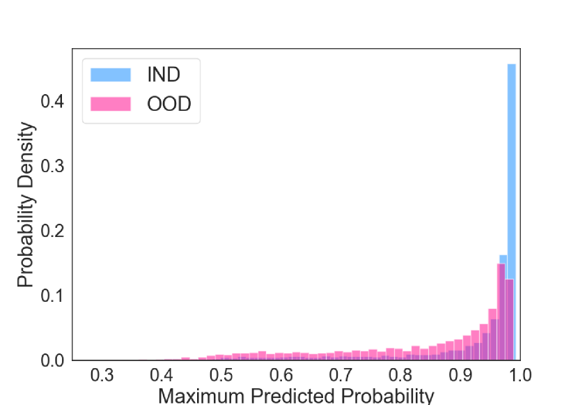
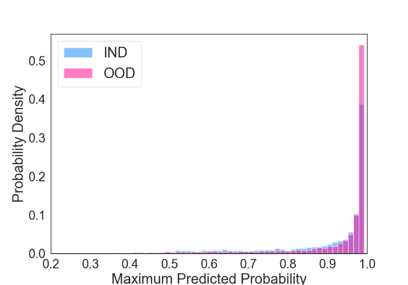
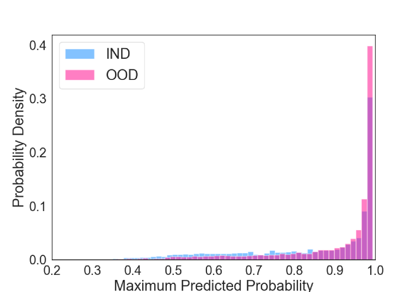
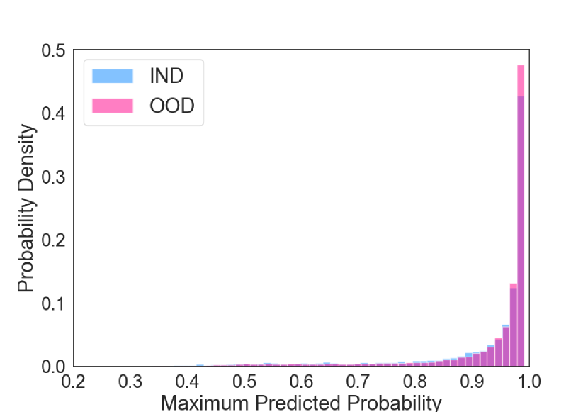
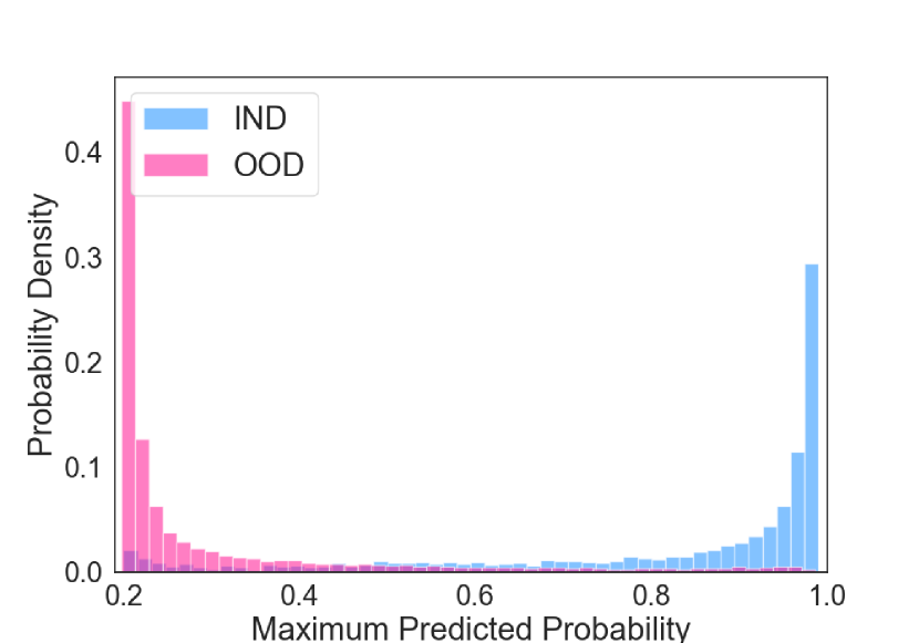
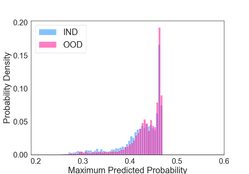
Results. The experimental results are shown in Table 2. Although the fine-tuned PLMs outperformed TFIDF-NB in terms of classification ability, their OOD detection performance fell short of expectation. In particular, they performed less than TFIDF-NB in the AG’s News dataset and entirely failed to detect the OOD in the Corona Tweets dataset while generating negative IOD values. Although the PLMs exhibited better results compared to TFIDF-NB in the Fake News dataset, the difference was not statistically significant apart from DistilBERT. Even ERNIE 2.0, which leverages both text form and external knowledge, failed to yield a promising result. Figure 1 depicts the distributions of the maximum predicted probability of TFIDF-NB and BERT-base on the AG’s News dataset. BERT-base produces very high confidence scores on OOD examples contrary to TFIDF-NB, which is capable of generating a low confidence score on OOD instances. Likewise, the experimental results reveal that PLMs are not competent in detecting OOD sentences when they are fine-tuned in downstream tasks. This supports our claim that PLMs suffer from the distribution collapse issue, which harms the model’s reliability.

4 NoiER: Noise Entropy Regularisation

The most suspicious cause of distribution collapse is the excessive exploitation of syntactic artifacts Niven and Kao (2019); McCoy et al. (2019). Therefore, improving the model’s generalisation ability by preventing the model from learning spurious artifacts is essential to overcome this issue. To this end, we applied the entropy regularisation (ER) technique, which has shown promising performance in improving the model’s robustness Hendrycks et al. (2019); Lee et al. (2018); Zheng et al. (2020). The question is which sentences could be leveraged for minimising the ER term. Collecting OOD instances is practically inefficient, as we illustrated in Section 2. Training an OOD sentence generator Lee et al. (2018); Zheng et al. (2020) also has the demerit that the model becomes highly contingent on the generator’s performance. Also, we have to retrain both the OOD sample generator and classifier whenever the distribution of training data changes, which is a time- and resource-intensive work.

To overcome the practical disadvantage, we decided to leverage a model-free approach by considering noise-added IND sentences as OOD data points. The role of the perturbed sentences is to assist the model with recognising the fact that a data point could be included in OOD even though it has analogous syntactic patterns with IND sentences. Hence, they should satisfy the following conditions:

Condition 1. A noise sentence should share a similar form with IND sentences to a certain extent.

Condition 2. Despite Condition 1, a noise sentence must be considered as OOD sentence.

4.1 Noise Generation Scheme

We used three noise generation functions: deletion, permutation Lample et al. (2018), and replacement.

1. Deletion: This function removes words in a sentence $s$ with the probability of $p_{del}$.

2. Permutation: This function shuffles at most $r_{perm}\%$ of words in a sentence $s$.

3. Replacement: This function replaces words in a sentence $s$ to randomly generated words with the probability of $p_{repl}$.

We distinguished the terminology “word” from “token”, because our approach focuses on generating noise on the word level rather than subword (i.e., token) level. Note that the noise generation methods are independent from the model’s tokenizer. Each noise function has its corresponding hyperparameters. We empirically found the optimum values for each dataset while analysing the IOD value of the validation dataset. More detailed explanations regarding the hyperparameter search are given in Appendix A.2.

Algorithm 1 Noise entropy regularisation training process for fine-tuning model $M_{\theta}$.

Input: An input sentence set $X=(x_{1},x_{2},...,x_{n})$, corresponding label set $Y=(y_{1},y_{2},...,y_{n})$, number of iterations $T$.
Output: A fine-tuned model $M_{\theta}$

1:for iter = 1, …, T do

2:     $X_{b},Y_{b}$ $\leftarrow$ BATCH(X,Y);

3:     ${\tilde{X_{b}}}$ $\leftarrow$ NOISE($X_{b}$);

4:     $\hat{Y}$ $\leftarrow$ $M_{\theta}(X_{b})$;

5:     $\mathcal{L}_{CE}$ $\leftarrow$ $\frac{1}{|X_{b}|}\sum_{y_{i}\in\hat{Y}}-y_{i}\log(\hat{y}_{i})$;

6:     $\mathcal{L}_{ER}$ $\leftarrow$ $\frac{1}{|\tilde{X_{b}}|}\sum_{\tilde{{x_{i}}}\in\tilde{X_{b}}}JSD(M_{\theta}(\tilde{x_{i}}),u)$;

7:     $\mathcal{L}\leftarrow\mathcal{L}_{CE}+\mathcal{L}_{ER}$;

8:     Update $\theta$ by descending its gradient $\nabla_{\theta}\mathcal{L}$

9:end for

4.2 Model Training

For each training iteration, we generated a noise sentence set $\tilde{X}_{b}$. Next, we leveraged $\tilde{X}_{b}$ to reduce the ER term. For a given model $M_{\theta}$, we defined the ER loss as the Jensen-Shannon divergence between the predicted probabilities and uniform distribution to reflect minimising the uniform disparity directly to our training objective:

$$\begin{gathered}\mathcal{L}_{ER}(\theta)=\sum_{\tilde{x_{i}}\in\tilde{X_{b}}}JSD(M_{\theta}(\tilde{x_{i}}),u),\end{gathered}$$ (5)

where $JSD$ and $u$ denote the Jensen-Shannon divergence and the uniform distribution, respectively. Finally, the final training loss is defined as the sum of the cross-entropy loss and the ER loss:

$$\begin{gathered}\mathcal{L}(\theta)=\mathcal{L}_{CE}(\theta)+\alpha\mathcal{L}_{ER}(\theta),\end{gathered}$$ (6)

where $\alpha$ is a hyperparameter, which is set to $\alpha=1$. The overall training process is shown in Algorithm 1.

Table 3: Results for the ablation study on DistilBert. The name of the dataset corresponds to IND. We trained each model 10 times and recorded the average of each metric. The best values are in bold. The notation “$\uparrow$” denotes that higher values are better, and “$\downarrow$” stands for lower values are better. For the IOD value, we multiplied the original figure with 100 to unify the scale with the other metrics. “Full” refers to leveraging the whole noise functions, whereas “w/o” denotes removing the following noise function.

Model	AG’s News				Fake News				Corona Tweets
	F1$\uparrow$	IOD$\uparrow$	AUROC$\uparrow$	EER$\downarrow$	F1$\uparrow$	IOD$\uparrow$	AUROC$\uparrow$	EER$\downarrow$	F1$\uparrow$	IOD$\uparrow$	AUROC$\uparrow$	EER$\downarrow$
Full	93.46	23.54	87.57	19.40	98.92	13.90	83.51	24.19	91.24	36.97	92.43	14.54
w/o Deletion	93.44	35.02	91.47	16.08	99.35	20.22	81.55	28.66	91.26	18.24	79.17	28.59
w/o Permutation	92.99	17.16	83.63	23.72	99.02	11.67	82.58	25.32	90.58	38.07	93.41	13.41
w/o Replacement	92.45	13.54	76.27	28.82	98.85	9.54	75.99	31.55	91.94	40.09	93.71	12.69
only Deletion	91.98	5.48	64.55	38.44	98.77	6.33	71.75	34.52	90.58	41.28	94.96	10.69
only Permutation	93.22	14.86	76.33	29.75	98.83	7.53	59.35	46.53	92.32	20.76	78.77	28.54
only Replacement	94.13	38.37	93.57	13.97	99.17	20.28	83.81	27.97	92.86	8.85	70.60	35.86

Table 4: Results for the comparison with the original fine-tuning framework. The name of the dataset corresponds to IND. We trained each model 10 times and recorded the average of each metric. For each pre-trained models, the best evaluation metric values are in bold. The notation “$\uparrow$” denotes that higher values are better, and “$\downarrow$” stands for lower values are better. “Full” refers to using all noise functions, whereas “Best” denotes the noise function combination that showed the best OOD detection performance. For the IOD value, we multiplied the original figure with 100 to unify the scale with the other metrics. Our proposed approach outperforms original fine-tuned models with $p$-value $<$ 0.05 ($\dagger$) and $p$-value $<$ 0.01 (*) using the t-test.

Model

AG’s News

Fake News

Corona Tweets

F1$\uparrow$

IOD$\uparrow$

AUROC$\uparrow$

EER$\downarrow$

F1$\uparrow$

IOD$\uparrow$

AUROC$\uparrow$

EER$\downarrow$

F1$\uparrow$

IOD$\uparrow$

AUROC$\uparrow$

EER$\downarrow$

BERT

Original

89.40

7.25

76.96

30.48

98.55

0.64

58.06

44.89

83.17

-2.13

40.65

57.51

Ours-Full

88.39*

18.68*

80.60$\dagger$

27.16$\dagger$

97.81*

13.52*

80.44*

27.44*

81.70*

30.33*

86.52*

22.64*

Ours-Best

89.08

33.26*

91.62*

16.94*

98.08*

17.52*

82.39*

29.38*

80.77*

35.95*

90.82*

16.80

DistilBERT

Original

89.82

7.35

75.87

31.20

98.62

1.48

59.94

44.64

81.61

-2.24

41.63

57.02

Ours-Full

88.52*

18.75*

82.08*

25.12*

97.89*

10.34*

76.56*

30.39*

80.72

33.15*

88.85*

19.25*

Ours-Best

88.96*

37.52*

92.87*

14.24*

98.02*

17.20*

80.19*

30.55*

80.23$\dagger$

37.48*

92.58*

13.78*

Electra

Original

88.91

7.12

79.05

28.11

98.48

1.91

57.14

47.79

82.05

-1.85

42.28

56.61

Ours-Full

88.11*

17.24*

79.85

27.58

97.93*

10.12*

76.09*

32.89*

81.34

30.73*

86.38*

22.26*

Ours-Best

88.61

35.74*

91.97*

15.65*

98.16$\dagger$

15.40*

79.77*

32.52*

81.49

34.39*

89.24*

19.01*

SqueezeBERT

Original

88.93

6.68

76.65

30.53

98.33

1.96

59.94

45.06

82.01

-1.85

41.87

56.43

Ours-Full

88.16*

16.34*

79.25$\dagger$

27.98$\dagger$

97.78$\dagger$

9.83*

75.84*

32.42*

81.52

27.29*

83.73*

25.25*

Ours-Best

88.67*

35.73*

91.67*

16.26*

98.30

13.78*

76.55*

35.01*

80.76*

36.16*

90.80*

17.16*

ERNIE 2.0

Original

89.45

5.85

73.78

33.07

98.56

1.82

50.72

53.06

82.12

-2.13

41.00

56.75

Ours-Full

87.96*

18.54*

81.24*

26.19*

97.95*

12.71*

78.24*

28.93*

77.85*

28.52*

86.85*

21.41*

Ours-Best

88.46*

33.77*

91.47*

16.28*

97.95*

15.89*

79.32*

31.98*

80.33*

35.97*

91.21*

16.32*

5 Experiments

We conducted experiments to confirm the effectiveness of the proposed approach under the same experimental design illustrated in Section 3.2.

Table 5: Results for the comparison with baseline models. The name of the dataset corresponds to IND. We trained each model 10 times and recorded the average of each metric. The best value is in bold. NoiER-DistilBERT-Best showed a statistically significant difference compared to other models with $p$-value $<$ 0.05 ($\dagger$) and $p$-value $<$ 0.01 (*) using the t-test. The notation $\uparrow$ denotes that higher values are better, and $\downarrow$ stands for lower values are better. For the IOD value, we multiplied the original figure with 100 to unify the scale with the other metrics.

Model

AG’s News

Fake News

Corona Tweets

F1$\uparrow$

IOD$\uparrow$

AUROC$\uparrow$

EER$\downarrow$

F1$\uparrow$

IOD$\uparrow$

AUROC$\uparrow$

EER$\downarrow$

F1$\uparrow$

IOD$\uparrow$

AUROC$\uparrow$

EER$\downarrow$

MSP-Linear

76.75*

7.61*

70.33*

35.29*

95.07*

5.55*

62.29*

41.73*

45.58*

2.04*

52.76*

48.14*

MSP-DistilBERT

89.82*

7.25*

76.96*

30.48*

98.62*

1.48*

59.94*

44.64*

81.61$\dagger$

-2.24*

41.63*

57.02*

ODIN-Linear

76.75*

7.63*

70.38*

35.29*

95.07*

5.55*

62.30*

41.73*

45.54*

2.05*

52.78*

48.14*

ODIN-DistilBERT

89.83*

7.25*

76.97*

30.47*

98.63*

1.48*

59.97*

44.62*

81.61$\dagger$

-2.24*

41.66*

57.02*

AE-BiLSTMSA

87.11*

-

83.74*

24.38*

97.90

-

52.22*

49.65*

74.31*

-

68.65*

35.97*

AE-DistilBERT

89.82*

-

77.37*

28.97*

98.62*

-

57.60*

45.35*

81.61$\dagger$

-

42.51*

55.22*

ERPOG-DistilBERT

85.11*

22.66*

84.66*

22.98*

94.10*

-5.11*

38.22*

63.08*

29.29*

-5.02*

26.80*

71.53*

GER-DistilBERT

89.51*

0.73*

72.26*

32.87*

98.32$\dagger$

0.29*

59.60*

46.49*

81.34$\dagger$

-0.50*

44.30*

54.86*

CNER-DistilBERT

89.09

3.73*

71.39*

35.37*

97.30*

1.81*

46.59*

55.05*

78.72

-2.95*

40.13*

58.16*

NoiER-DistilBERT-Full

88.52$\dagger$

18.75*

82.08*

25.12*

97.89

10.34*

76.56

30.39

80.72

33.15*

88.85*

19.25*

NoiER-DistilBERT-Best

88.96

37.52

92.87

14.24

98.02

17.20

80.19

30.55

80.23

37.48

92.58

13.78

5.1 Ablation Study

We first performed an ablation study to figure out the influence of noise generation functions. We used DistilBERT for this study, because of its low model complexity, and all PLMs exhibited a similar trend in Table 2. The experiment was conducted for every possible combination of noise functions. For a fair comparision, we used the validation dataset to decide the best combination. The results are summarised in Table 3. We observed that the best combination varies for each dataset. In detail, using the “only Deletion” function was the most efficient for the Corona Tweets. For the AG’s News and Fake News dataset, the “only Replacement” function produced the best results. In addition, using only “Deletion” or “Permutation” has almost no impact on improving the OOD detection performance. We give further explanations regarding this phenomenon in Appendix A.5.

5.2 Comparison with Fine-tuned Models

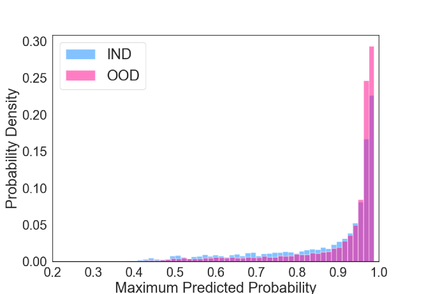
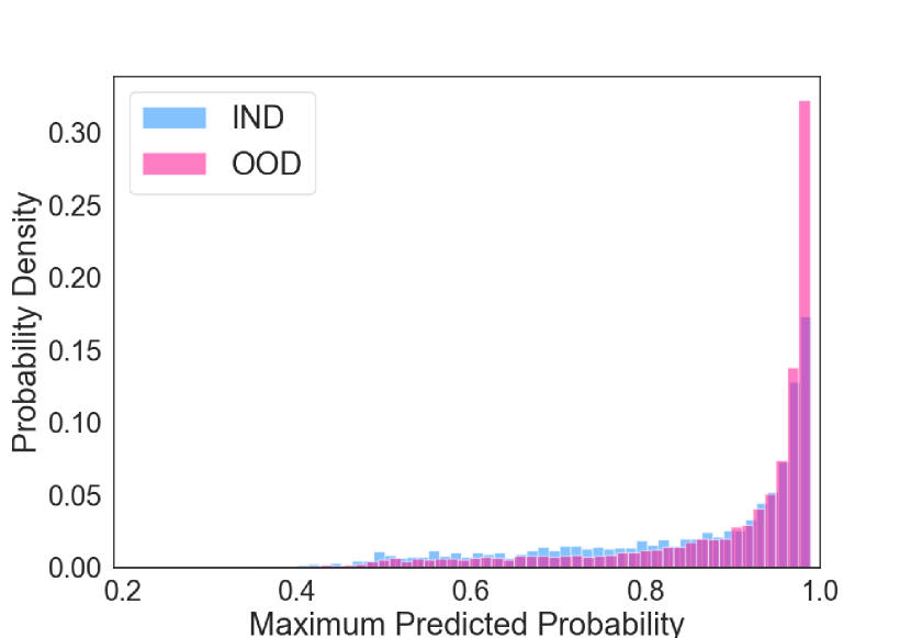
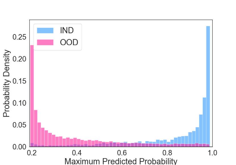
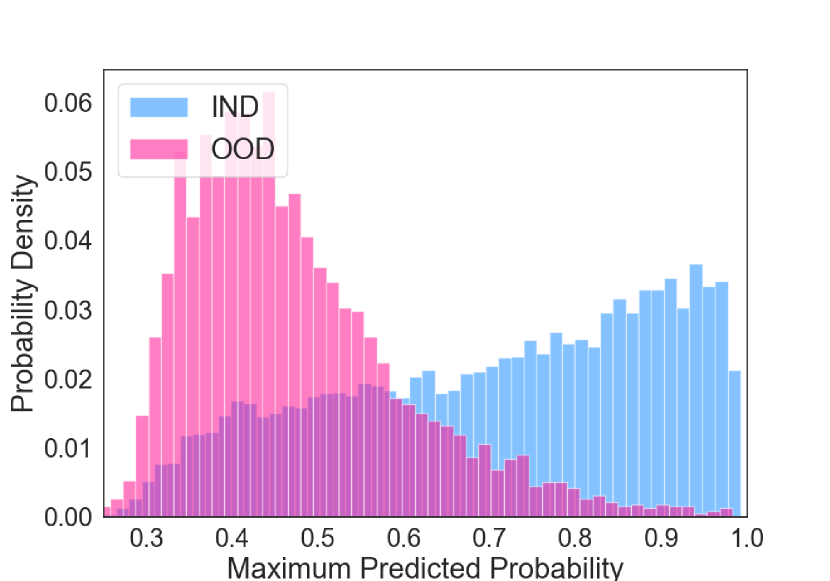
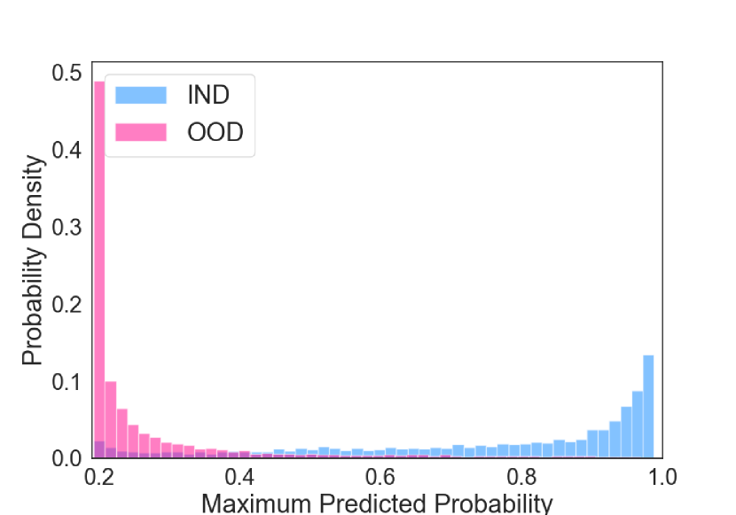
The second experiment is comparing the performance of our proposed approach with that of the originally fine-tuned LMs. The results are summarised in Table 4. We recorded the results of the “Full” model and the best noise function combination for each PLMs. Through the experiments, we confirmed that the “Full” model guarantees an improvement on the OOD detection ability regardless of the dataset and PLMs. Although the F1-score is marginally reduced by 1.1% on average, the decrease is negligible, considering the promising improvement in OOD detection performance. Specifically, for the “Full” model case, the AUROC and EER values increased by 50% and 36% on average, respectively. For the “Best” case, the metrics were improved by 60% and 49% on average, respectively. The outperforming OOD detection ability of our proposed approach can also be verified by the distribution plots in Figure 2.

(a) DistilBERT-base

(b) NoiER-DistilBERT-Best

Figure 2: Maximum predicted probability distribution plots when the Corona Tweets dataset is IND.

5.3 Comparison with Baseline Models

Finally, we conducted an experimental comparison with other baseline approaches. For a fair comparison, we selected OOD detectors that could be applied to PLMs while using IND data only. We used DistilBERT Sanh et al. (2019) as a backbone pretrained model of this study because of its lower training time. The details of the baseline candidates are illustrated below.

1. MSP Hendrycks and Gimpel (2017): We trained two variations of this approach, the original linear classifier (MSP-Linear) and the DistilBERT-based classifier (MSP-DistilBERT).

2. ODIN Liang et al. (2018): We applied this method to MSP-Linear and MSP-DistilBERT, which are denoted ODIN-Linear and ODIN-DistilBERT, respectively. We used the same search space of Liang et al. (2018) for selecting the hyperparameters.

3. AE Ryu et al. (2017): Although the authors used a BiLSTM classifier, we replaced it with a BiLSTM-Self Attention model Lin et al. (2017) (AE-BiLSTMSA) because of the original model’s low performance on the Corona Tweets dataset. We also applied this method to DistilBERT (AE-DistilBERT).

4. ERPOG Zheng et al. (2020): We applied this method to DistilBERT, which is denoted ERPOG-DistilBERT.

5. Variants of our approach: We additionally trained two variants of our approach. The first one is using IND sentences for minimising the ER term. This model can be considered as a special case of generalised entropy regularisation Meister et al. (2020). The second model adds continuous Gaussian noise to the distributed sentence representations Zhang and Yang (2018). We denote the aforementioned baselines GER-DistilBERT and CNER-DistilBERT, respectively.

Table 5 describes the comparison results. The IOD value of AE models are omitted, because they detect OOD by using reconstruction errors. The results reveal that the proposed approach better detects OOD compared to the baselines. The results show that our approach is capable of detecting OOD instances well for all datasets. For the AG’s News dataset, AE-BiLSTMSA and ERPOG-DistilBERT produced promising results among the baselines. They exhibited comparable but slightly better results compared to the “Full” model of our approach in terms of OOD detection ability. However, all the baseline models fell short of distinguishing OOD instances in the Fake News and Corona Tweets dataset. In particular, ERPOG-DistilBERT entirely failed to detect OOD in both datasets. We suspect that this result stems from the relatively longer sentence length compared to the AG’s News dataset. The performance of the LSTM-based Seq2Seq model dwindles as the length of the sequence goes longer Bahdanau et al. (2015), which leads the pseudo-OOD generator to produce defective sentences. Therefore, the ERPOG model is trained with corrupted sentences, which inevitably degrades both the classification and the OOD detection performance. This result reveals the drawback of OOD generator-based approaches.

It is also worth mentioning that the variants of our approach have no impact on the OOD detection performance. Notably, generating continuous noise samples aggravated the distribution collapse issue. This may be due to the natural structure of text data as a discrete token sequence, which makes them suffer from latent vacancy problem Xu et al. (2020). Likewise, the experimental results demonstrate our approach’s effectiveness, which leverages discrete pseudo OOD examples generated in a model-free way.

6 Summary and Outlook

In this paper, we have shown that the distribution collapse is a prevalent issue that frequently occurs in PLMs. This is a problematic issue, because it degrades the reliability of the models. To solve this issue, we propose a simple but effective approach: noise entropy regularisation. The proposed method generates noise sentences, which share a similar syntactic form with IND sentences, and leverages them to minimise entropy regularisation loss. Extensive experiments reveal that the proposed approach significantly improves the OOD detection ability of the original PLMs, while preserving their high performance on classification. Also, it outperforms baseline models designed for OOD text detection. Moreover, our approach is advantageous in terms of its practicality, because additional data or auxiliary models are unnecessary.

As for future works, an interesting topic is to expand our approach to sequential labeling tasks, such as named entity recognition (NER). Also, our approach has a drawback in that it relies on the randomised process, which could generate different outcomes for each training process. Therefore, implementing a more stable method is another interesting research direction.

Appendix A Supplemental Material

A.1 Evaluation Metrics

In addition to the IOD value, we leveraged two widely used metrics: AUROC and EER for measuring OOD detection performance. AUROC is the area under the receiver operating characteristic curve, which is created by plotting the true positive rate (TPR) against the false positive rate (FPR) at diverse levels of thresholds Chen et al. (2005). EER is the intersection point where the false rejection rate (FRR) and the false acceptance rate (FAR) meet Kim et al. (2021). Therefore, lower EER values imply that a model is more accurate.

A.2 Hyperparameter Search

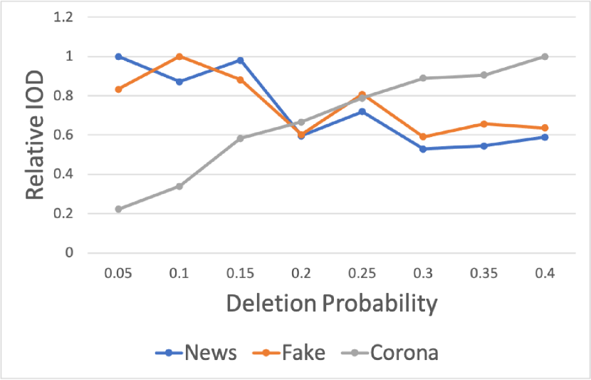
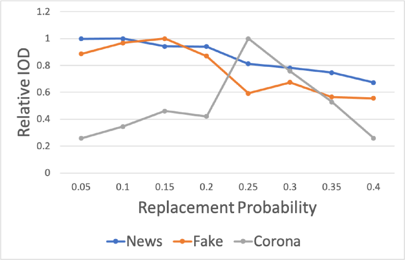
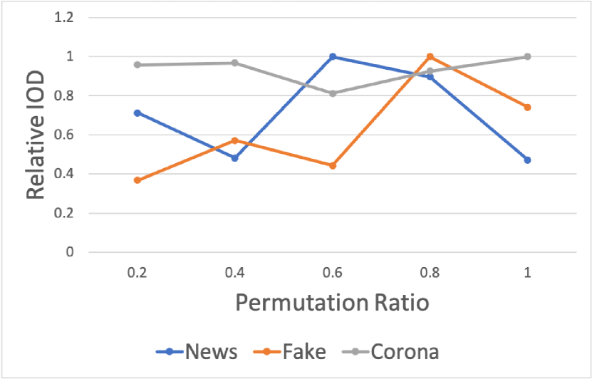
In this section, we present more detailed explanations regarding the noise function’s hyperparameter search. We have three hyperparameters to decide: $p_{del}$, $p_{repl}$, and $r_{perm}$ for deletion, replacement, and permutation, respectively. For the probability $p_{del}$ and $p_{repl}$, we choose from evenly spaced 8 numbers starting from 0.05 and ending at 0.4. For the ratio $r_{perm}$, we select among 0.2, 0.4, 0.6, 0.8, and 1.0. To decide the optimum figures, we leveraged the IOD value of the validation dataset, which is independent from the test dataset. We repeated the training 10 times for each hyperparameter setting and leveraged DistilBERT as a backbone model. Figure 4 presents the relative average IOD values on the hyperparameter settings for each noise functions. The selected values are summarised in Table 6. We found that there exists a strong correlation between the average length of the sentences included in the dataset and the noise generation hyperparameter values. We conjecture that this is because the high noise parameter values on short sentences significantly change the IND sentences, violating Condition 1 in Section 4. On the contrary, low noise parameter values on long sentences make IND and perturbed sentences indistinguishable, which violates Condition 2.

A.3 Correlation between IOD and AUROC

A text classification model that possesses a good OOD detection ability should produce high IOD and AUROC scores. However, this does not imply that the IOD value has a positive correlation with the AUROC score. The model that produces a high IOD value also generates a high AUROC score. However, the vice versa case does not hold in a certain situation. This is because the IOD value merely measures the distribution disparity, whereas AUROC is an evaluation metric that belongs to the accuracy category.

Table 6: Summary of the selected hyper-parameters

	AG’s News	Fake News	Corona Tweets
$p_{del}$	0.05	0.1	0.4
$p_{repl}$	0.1	0.15	0.25
$r_{perm}$	0.6	0.8	1.0

(a) low IOD but high AUROC

Figure 3: Maximum predicted probability distribution plot for explaining uncorrelatedness between IOD and AUROC.

(a) Deletion ($p_{del}$)

(b) Replacement ($p_{repl}$)

(c) Permutation ($r_{perm}$)

Figure 4: Plots for the relative average IOD values for deciding hyper-parameters of noise generation functions.

(a) AG’s News

(b) Fake News

(c) Corona Tweets

Figure 5: Maximum predicted probability distribution plots of GER-DistilBERT.

Algorithm 2 Generating noise sentences.

Input: An input sentence $s=(w_{1},w_{2},...,w_{n})$, where $w_{i}$ is an $i^{th}$ word of the sentence $s$. The hyperparameters: $p_{del}$, $p_{repl}$, and $r_{perm}$.
Output: A noise-added sentence

1:$\hat{s}$ $\leftarrow$ COPY($s$)$\triangleright$ Copy the input

2:while $s==\hat{s}$ do

3:     $p$ $\leftarrow$ UNIFORM(0,1)

4:     if $p$ $\leq\frac{1}{3}$  then $\triangleright$ Delete words

5:         s $\leftarrow$ DELETEWORD(s, $p_{del}$)

6:     else if $p$ $\geq\frac{2}{3}$ then $\triangleright$ Permute words

7:         L $\leftarrow$ len(s)

8:         s $\leftarrow$ PERMUTEWORD(s, $r_{perm}$)

9:     else$\triangleright$ Replace words

10:         s $\leftarrow$ REPLACEWORD(s, $p_{repl}$)

11:     end if

12:end while

A.3.1 Low IOD but High AUROC

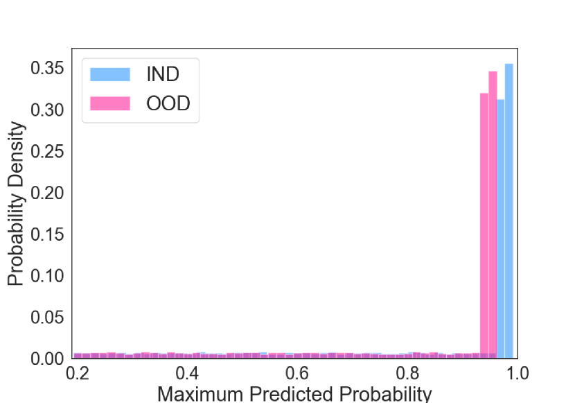
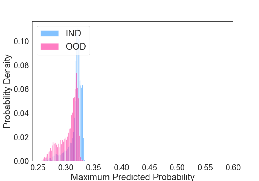
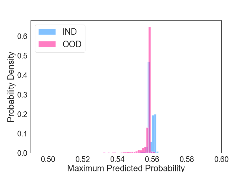
Figure 3(a) well illustrates the corresponding situation. In this example, the AUROC score is quite high, because we can distinguish IND and OOD examples, provided we set a threshold to about 0.95. However, the IOD value is close to 0, because the two distributions are almost similar. In our experiments, the results of GER-DistilBERT on the AG’s News and Fake News dataset, which are provided in Table 5 and Figure 5, correspond to this case.

Although a model can generate a high AUROC score but a low IOD value, it is obvious that a model that produces both a high IOD value and a high AUROC score is a better classification model, because it is much easier to set a threshold for rejecting OOD. Therefore, both metrics have to be considered to fully evaluate the model’s OOD detection performance.

A.4 Noise Generation Algorithm

The overall process for generating noise sentences is described in Algorithm 2. It randomly decides one function from the three candidates. For the ablation study, we manipulated the random probability $p$ to prevent certain functions from being selected.

Table 7: Generated noise examples for the AG’s News dataset

Original sentence	Label	Generated noise
HP shares tumble on profit news	Business	Del	HP shares tumble profit news
		Permute	HP tumble shares on news profit
		Repl	7Z shares tumble GE profit news
How mars fooled the world	Sci/Tech	Del	How mars fooled world
		Permute	mars How fooled the world
		Repl	06B mars fooled the SD8EG
Venezuela opposition holds recall vote	World	Del	Venezuela opposition recall vote
		Permute	opposition Venezuela holds recall vote
		Repl	Venezuela opposition holds 0MUFHF vote
Basketball: China #39;s Yao takes anger out on New Zealand	Sports	Del	Basketball: china #39;s Yao takes out on New Zealand
		Permute	China basketball: #39;s anger out Yao takes New on Zealand
		Repl	Basketball: HRTE5 #39;s Yao takes anger out on New FZH611A

A.5 Ablation Study Result Analysis

In this section, we describe a more detailed explanation of the ablation study results. The notable characteristic is that the “Deletion” and “Permutation” functions are unprofitable, or even worse, work negatively on the AG’s News and Fake News dataset. We conjecture that this phenomenon is due to the length of the input sentence. As illustrated in Appendix A.2, the shorter the input sentence is, the fewer noise is added to prevent violating Condition 1 in Section 4. However, unlike the “Replacement” function, which introduces external words into the sentence, “Deletion” and “Permutation” functions only reorganise words within a sentence. These characteristics inevitably increase the possibility of the sentence being considered as IND. As a result, Condition 2, in Section 4 is violated, which causes a negative influence on the model’s OOD detection ability. Table 7 contains the examples of generated noise sentences on the AG’s News dataset. Unlike the “Replacement” function, considering the result of the “Deletion” and “Permutation” functions as OOD sentences is not reasonable.

The experimental results presented in Table 3 also support the relationship between the input sentence’s length and the effect of the “Deletion” and “Permutation” functions. For the AG’s News dataset, both the “only Deletion” and the “only Permutation” model significantly performed less than the original fine-tuned model under 0.01 confidence level. However, when it comes to the Fake News dataset, the “only Deletion” model’s results showed no difference with the original fine-tuned model. Although the “only Permutation” model did not perform well again, it produced a higher $p$-value. Finally, for the Corona Tweets dataset, both the “only Deletion” and the “only Permutation” model outperformed the original fine-tuned model under 0.01 confidence level. Therefore, we recommend users to remove the “Deletion” and “Permutation” functions, if the dataset that they use to apply our approach on contains many short sentences.

A.6 Example Graphs

We added examples of the maximum predicted probability distribution plots of original fine-tuned models and those of our proposed approach. Figures 6 and 7 present the distribution plots of the fine-tuned models and the NoiER approach on the Corona Tweets dataset. It can be easily seen that the proposed approach distinguishes OOD sentences much better than the original fine-tuned models.

(a) BERT-base

(b) DistilBERT-base

(c) ELECTRA

(d) SqueezeBERT

(e) ERNIE 2.0

Figure 6: Maximum predicted probability distribution plots of original fine-tuned models when Corona Tweets data are IND.

(a) BERT-base

(b) DistilBERT-base

(c) ELECTRA

(d) SqueezeBERT

(e) ERNIE 2.0

Figure 7: Maximum predicted probability distribution plots of NoiER-BEST models when Corona Tweets data are IND.

References

- Ahmed et al. (2017) Hadeer Ahmed, Issa Traore, and Sherif Saad. 2017. Detection of online fake news using n-gram analysis and machine learning techniques. In Intelligent, Secure, and Dependable Systems in Distributed and Cloud Environments, pages 127–138, Cham. Springer International Publishing.
- Amodei et al. (2016) Dario Amodei, Chris Olah, Jacob Steinhardt, Paul Christiano, John Schulman, and Dan Mané. 2016. Concrete problems in ai safety. arXiv preprint arXiv:1606.06565.
- Bahdanau et al. (2015) Dzmitry Bahdanau, Kyunghyun Cho, and Yoshua Bengio. 2015. Neural machine translation by jointly learning to align and translate. International Conference on Learning Representations.
- Bender and Koller (2020) Emily M. Bender and Alexander Koller. 2020. Climbing towards NLU: On meaning, form, and understanding in the age of data. In Proceedings of the 58th Annual Meeting of the Association for Computational Linguistics, pages 5185–5198, Online. Association for Computational Linguistics.
- Chen et al. (2005) Wun-Hwa Chen, Sheng-Hsun Hsu, and Hwang-Pin Shen. 2005. Application of svm and ann for intrusion detection. Computers & Operations Research, 32(10):2617–2634.
- Clark et al. (2020) Kevin Clark, Minh-Thang Luong, Quoc V. Le, and Christopher D. Manning. 2020. ELECTRA: Pre-training text encoders as discriminators rather than generators. In International Conference on Learning Representations.
- Devlin et al. (2018) Jacob Devlin, Ming-Wei Chang, Kenton Lee, and Kristina Toutanova. 2018. BERT: Pre-training of deep bidirectional transformers for language understanding. arXiv preprint arXiv:1810.04805.
- Goodfellow et al. (2015) Ian J Goodfellow, Jonathon Shlens, and Christian Szegedy. 2015. Explaining and harnessing adversarial examples. International Conference on Learning Representations.
- Habernal et al. (2018) Ivan Habernal, Henning Wachsmuth, Iryna Gurevych, and Benno Stein. 2018. The argument reasoning comprehension task: Identification and reconstruction of implicit warrants. In NAACL-HLT.
- Harrou et al. (2016) Fouzi Harrou, Ying Sun, and Sofiane Khadraoui. 2016. Amalgamation of anomaly-detection indices for enhanced process monitoring. Journal of Loss Prevention in the Process Industries, 40:365 – 377.
- Hendrycks and Gimpel (2017) Dan Hendrycks and Kevin Gimpel. 2017. A baseline for detecting misclassified and out-of-distribution examples in neural networks. International Conference on Learning Representations.
- Hendrycks et al. (2019) Dan Hendrycks, Mantas Mazeika, and Thomas Dietterich. 2019. Deep anomaly detection with outlier exposure. International Conference on Learning Representations.
- Iandola et al. (2020) Forrest Iandola, Albert Shaw, Ravi Krishna, and Kurt Keutzer. 2020. SqueezeBERT: What can computer vision teach nlp about efficient neural networks? In Proceedings of SustaiNLP: Workshop on Simple and Efficient Natural Language Processing, pages 124–135.
- Kim et al. (2021) Czangyeob Kim, Myeongjun Jang, Seungwan Seo, Kyeongchan Park, and Pilsung Kang. 2021. Intrusion detection based on sequential information preserving log embedding methods and anomaly detection algorithms. IEEE Access, 9:58088–58101.
- Kim and Kim (2018) Joo-Kyung Kim and Young-Bum Kim. 2018. Joint learning of domain classification and out-of-domain detection with dynamic class weighting for satisficing false acceptance rates. Proc. Interspeech 2018, pages 556–560.
- Lample et al. (2018) Guillaume Lample, Alexis Conneau, Ludovic Denoyer, and Marc’Aurelio Ranzato. 2018. Unsupervised machine translation using monolingual corpora only. International Conference on Learning Representations.
- Lee et al. (2018) Kimin Lee, Honglak Lee, Kibok Lee, and Jinwoo Shin. 2018. Training confidence-calibrated classifiers for detecting out-of-distribution samples. International Conference on Learning Representations.
- Liang et al. (2018) Shiyu Liang, Yixuan Li, and Rayadurgam Srikant. 2018. Enhancing the reliability of out-of-distribution image detection in neural networks. International Conference on Learning Representations.
- Lin et al. (2017) Zhouhan Lin, Minwei Feng, Cicero Nogueira dos Santos, Mo Yu, Bing Xiang, Bowen Zhou, and Yoshua Bengio. 2017. A structured self-attentive sentence embedding. International Conference on Learning Representations.
- Loshchilov and Hutter (2018) Ilya Loshchilov and Frank Hutter. 2018. Decoupled weight decay regularization. In International Conference on Learning Representations.
- McCoy et al. (2019) Tom McCoy, Ellie Pavlick, and Tal Linzen. 2019. Right for the wrong reasons: Diagnosing syntactic heuristics in natural language inference. In Proceedings of the 57th Annual Meeting of the Association for Computational Linguistics, pages 3428–3448.
- Meister et al. (2020) Clara Meister, Elizabeth Salesky, and Ryan Cotterell. 2020. Generalized entropy regularization or: There’s nothing special about label smoothing. arXiv preprint arXiv:2005.00820.
- Niven and Kao (2019) Timothy Niven and Hung-Yu Kao. 2019. Probing neural network comprehension of natural language arguments. In Proceedings of the 57th Annual Meeting of the Association for Computational Linguistics, pages 4658–4664.
- Oh et al. (2018) K. Oh, D. Lee, C. Park, Y. Jeong, S. Hong, S. Kwon, and H. Choi. 2018. Out-of-domain detection method based on sentence distance for dialogue systems. In 2018 IEEE International Conference on Big Data and Smart Computing (BigComp), pages 673–676.
- Ohsugi et al. (2019) Yasuhito Ohsugi, Itsumi Saito, Kyosuke Nishida, Hisako Asano, and Junji Tomita. 2019. A simple but effective method to incorporate multi-turn context with bert for conversational machine comprehension. In Proceedings of the First Workshop on NLP for Conversational AI, pages 11–17.
- Peters et al. (2018) Matthew E. Peters, Mark Neumann, Mohit Iyyer, Matt Gardner, Christopher Clark, Kenton Lee, and Luke Zettlemoyer. 2018. Deep contextualized word representations. In Proceedings of NAACL-HLT, pages 2227–2237.
- Radford et al. (2018) Alec Radford, Karthik Narasimhan, Tim Salimans, and Ilya Sutskever. 2018. Improving language understanding by generative pre-training.
- Rajpurkar et al. (2016) Pranav Rajpurkar, Jian Zhang, Konstantin Lopyrev, and Percy Liang. 2016. SQuAD: 100,000+ questions for machine comprehension of text. In Proceedings of the 2016 Conference on Empirical Methods in Natural Language Processing, pages 2383–2392.
- Ryu et al. (2017) Seonghan Ryu, Seokhwan Kim, Junhwi Choi, Hwanjo Yu, and Gary Geunbae Lee. 2017. Neural sentence embedding using only in-domain sentences for out-of-domain sentence detection in dialog systems. Pattern Recognition Letters, 88:26–32.
- Ryu et al. (2018) Seonghan Ryu, Sangjun Koo, Hwanjo Yu, and Gary Geunbae Lee. 2018. Out-of-domain detection based on generative adversarial network. In Proceedings of the 2018 Conference on Empirical Methods in Natural Language Processing, pages 714–718.
- Sanh et al. (2019) Victor Sanh, Lysandre Debut, Julien Chaumond, and Thomas Wolf. 2019. DistilBERT, a distilled version of BERT: Smaller, faster, cheaper and lighter. arXiv preprint arXiv:1910.01108.
- Seo et al. (2020) Seungwan Seo, Deokseong Seo, Myeongjun Jang, Jaeyun Jeong, and Pilsung Kang. 2020. Unusual customer response identification and visualization based on text mining and anomaly detection. Expert Systems with Applications, 144:113111.
- Song and Suh (2019) Bomi Song and Yongyoon Suh. 2019. Narrative texts-based anomaly detection using accident report documents: The case of chemical process safety. Journal of Loss Prevention in the Process Industries, 57:47 – 54.
- Srivastava et al. (2014) Nitish Srivastava, Geoffrey Hinton, Alex Krizhevsky, Ilya Sutskever, and Ruslan Salakhutdinov. 2014. Dropout: A simple way to prevent neural networks from overfitting. Journal of Machine Learning Research, 15(56):1929–1958.
- Sun et al. (2020) Yu Sun, Shuohuan Wang, Yu-Kun Li, Shikun Feng, Hao Tian, Hua Wu, and Haifeng Wang. 2020. ERNIE 2.0: A continual pre-training framework for language understanding. In Proceedings of AAAI, pages 8968–8975.
- Xu et al. (2019) Hu Xu, Bing Liu, Lei Shu, and P. Yu. 2019. Open-world learning and application to product classification. In The World Wide Web Conference, pages 3413–3419.
- Xu et al. (2020) Peng Xu, Jackie Chi Kit Cheung, and Yanshuai Cao. 2020. On variational learning of controllable representations for text without supervision. In International Conference on Machine Learning, pages 10534–10543. PMLR.
- Yang et al. (2019) Zhilin Yang, Zihang Dai, Yiming Yang, Jaime Carbonell, Russ R. Salakhutdinov, and Quoc V. Le. 2019. Xlnet: Generalized autoregressive pretraining for language understanding. In Advances in Neural Information Processing Systems, pages 5753–5763.
- Zellers et al. (2018) Rowan Zellers, Yonatan Bisk, Roy Schwartz, and Yejin Choi. 2018. SWAG: A large-scale adversarial dataset for grounded commonsense inference. In Proceedings of the 2018 Conference on Empirical Methods in Natural Language Processing, pages 93–104.
- Zhang and Yang (2018) Dongxu Zhang and Zhichao Yang. 2018. Word embedding perturbation for sentence classification. arXiv preprint arXiv:1804.08166.
- Zhang et al. (2015) Xiang Zhang, Junbo Jake Zhao, and Yann LeCun. 2015. Character-level convolutional networks for text classification. In NIPS.
- Zheng et al. (2020) Yinhe Zheng, Guanyi Chen, and Minlie Huang. 2020. Out-of-domain detection for natural language understanding in dialog systems. IEEE/ACM Transactions on Audio, Speech, and Language Processing, 28:1198–1209.