Jet-temperature anisotropy revealed through high-$p_{\perp}$ data

Abstract

We explore to what extent, and how, high-$p_{\perp}$ data and predictions reflect the shape and anisotropy of the QCD medium formed in ultrarelativistic heavy-ion collisions. To this end, we use our recently developed DREENA-A framework, which can accommodate any temperature profile within the dynamical energy loss formalism. We show that the ratio of high-$p_{\perp}$ $v_{2}$ and $(1-R_{AA})$ predictions reaches a well-defined saturation value, which is directly proportional to the time-averaged anisotropy of the evolving QGP, as seen by the jets.

I Introduction

Quark-gluon plasma is a new form of matter created in ultrarelativistic heavy ion collisions. The main goal of relativistic heavy ion physics probe1 ; probe2 ; probe3 ; probe4 is to explore the properties of this new form of matter QGP1 ; QGP2 , which will in turn lead to a fundamental understanding of QCD matter at its basic level. In the QGP tomography approach that we advocate, the energy loss of rare high energy partons traversing the medium is used to map its properties.

We previously argued shapeQGP that, at large enough values of transverse momentum (high-$p_{\perp}$), the ratio of the elliptic flow parameter $v_{2}$ and $1-R_{AA}$, where $R_{AA}$ is the nuclear suppression factor, saturates, and reflects only the geometry of the system. This argument was based on analytic considerations and a simple 1-dimensional expansion Bjorken ; DREENAB . To see how the evolving shape of the collision system is reflected in the high-$p_{\perp}$ observables, we here study the behavior of $v_{2}/(1-R_{AA})$ in a system that expands both in longitudinal and transverse directions.

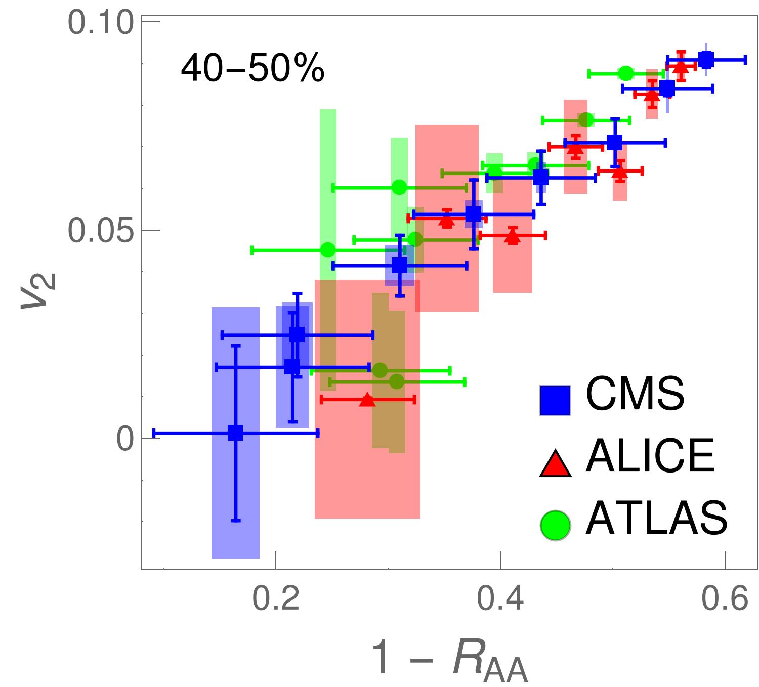
Furthermore, it has been experimentally observed that at high values of transverse momentum $v_{2}$ and $1-R_{AA}$ are directly proportional. This is shown in Fig. 1 for ALICE ALICE_CH_RAA ; ALICE_CH_v2 , CMS CMS_CH_RAA ; CMS_CH_v2 , and ATLAS ATLAS_CH_RAA ; ATLAS_CH_v2 data. Such relationship is equivalent to a $p_{\perp}$-independent ratio of $v_{2}$ and $1-R_{AA}$, and we study whether the fluid dynamical calculation can reproduce such proportionality, and whether we can relate this observation to a physical property of the system, namely to its anisotropy.

Figure 1: $v_{2}$ vs $1\!-\!R_{AA}$ for $p_{\perp}\!>\!10$ GeV data from 5.02 TeV Pb+Pb ALICE ALICE_CH_RAA ; ALICE_CH_v2 (red triangles), CMS CMS_CH_RAA ; CMS_CH_v2 (blue squares) and ATLAS ATLAS_CH_RAA ; ATLAS_CH_v2 (green circles) experiments. The data is shown for the 40-50% centrality bin, while similar relation is obtained for other centralities. Each collaboration’s datapoints correspond to different values of $p_{\perp}$, with both $v_{2}$ and $1\!-\!R_{AA}$ decreasing with increasing $p_{\perp}$.

As is the standard approach in the study of ultrarelativistic heavy-ion collisions, we assume the collision system to behave as a locally thermalized dissipative fluid. It is well known that the transverse expansion of such a system largely depends on the initial gradients of the system, i.e., the initial state, and also on the equation of state (EoS) and dissipative properties of the fluid. Thus, to provide more general conclusions about the asymptotic behavior of $v_{2}/(1-R_{AA})$, it is necessary to explore not only one, but several, different scenarios of fluid-dynamical evolution. On the other hand, to provide physically meaningful results, tuning the calculations to reproduce the observed low-$p_{\perp}$ data is necessary. As known, finding suitable parameter combinations is a considerable task, and therefore we do not explore the parameter space ourselves but employ various initializations, and corresponding parameter sets, presented in the literature. In particular, we restrict ourselves to models tuned to reproduce the Pb+Pb collisions at $\sqrt{s_{\mathrm{NN}}}=5.02$ TeV collision energy at the LHC. We further note that constraining the calculation to reproduce the low-$p_{\perp}$ data does not guarantee the reproduction of the high-$p_{\perp}$ data. Simultaneous reproduction of both is not an aim of this study, but left for future work.

We will see that the temperature evolution in different evolution scenarios is different enough to lead to observable differences in high-$p_{\perp}$ $v_{2}$ and $1-R_{AA}$, and the ratio of these observables is directly related to a suitably defined measure of the system anisotropy.

II Methods

II.1 Medium Evolution

Our starting point and reference is a simple optical Glauber model based initialization, which we use at different initial times $\tau_{0}=0.2,\,0.4,\,0.6,\,0.8$ and $1.0$ fm. The initialization and code used to solve viscous fluid-dynamical equations in 3+1 dimensions are described in detail in Ref. Molnar:2014zha , and parameters to describe Pb+Pb collisions at $\sqrt{s_{\mathrm{NN}}}=5.02$ TeV in Ref. Stojku:2020wkh . In particular, we use a constant shear viscosity to entropy density ratio $\eta/s=0.12$, and the EoS parametrization $s95p$-PCE-v1 Huovinen:2009yb .

Our second option, Glauber + Free streaming, is to use the Glauber model to provide the initial distribution of (marker) particles, allow the particles to stream freely from $\tau=0.2$ to $1.0$ fm, evaluate the energy-momentum tensor of these particles, and use it as the initial state of the fluid. We evolve the fluid using the same code as in the case of pure Glauber initialization. The EoS is $s95p$-PCE175, i.e., a parametrization with $T_{\mathrm{chem}}=175$ MeV Niemi:2015qia , and temperature-independent $\eta/s=0.16$. For further details, see Ref. Stojku:2020wkh .

As more sophisticated initializations, we employ EKRT, IP-Glasma and T_RENTo. The EKRT model Eskola:1999fc ; Paatelainen:2012at ; Paatelainen:2013eea is based on the NLO perturbative QCD computation of the transverse energy and a gluon saturation conjecture. We employ the same setup as used in Ref. Auvinen:2020mpc (see also Niemi:2015qia ), compute an ensemble of event-by-event fluctuating initial density distributions, average them, and use this average as the initial state of the fluid dynamical evolution. We again use the code of Molnar et al., Molnar:2014zha , but restricted to boost-invariant expansion. The shear viscosity over entropy density ratio is temperature dependent with favored parameter values from the Bayesian analysis of Ref. Auvinen:2020mpc . Initial time is $\tau_{0}=0.2$ fm, and the EoS is the $s83s_{18}$ parametrization from Ref. Auvinen:2020mpc .

IP-Glasma model ipglasma ; ipglasma2 is based on Color Glass Condensate Iancu:2002xk ; Iancu:2003xm ; Gelis:2010nm ; Lappi:2010ek . It calculates the initial state as a collision of two color glass condensates and evolves the generated fluctuating gluon fields by solving classical Yang-Mills equations. The calculated event-by-event fluctuating initial states Schenke:2020mbo were further evolved Chun-private using the MUSIC code Schenke:2010nt ; Schenke:2010rr ; Schenke:2011bn constrained to boost-invariant expansion. We subsequently averaged the evaluated temperature profiles to obtain one average profile per centrality class. In these calculations, the switch from Yang-Mills to fluid-dynamical evolution took place at $\tau_{\mathrm{switch}}=0.4$ fm, shear viscosity over entropy density ratio was constant $\eta/s=0.12$, and the temperature-dependent bulk viscosity coefficient over entropy density ratio had its maximum value $\zeta/s=0.13$. The equation of state was based on the HotQCD lattice results HotQCD:2014kol as presented in Ref. Moreland:2015dvc .

T_RENTo Moreland:2014oya is a phenomenological model capable of interpolating between wounded nucleon and binary collision scaling, and with a proper parameter value, of mimicking the EKRT and IP-Glasma initial states. As with the EKRT initialization, we create an ensemble of event-by-event fluctuating initial states, sort them into centrality classes, average, and evolve these average initial states. Unlike in other cases, we employ the version of the VISH2+1 code Song:2007ux described in Refs. Bernhard:2018hnz ; Bernhard:2019bmu . We run the code using the favored values of the Bayesian analysis of Ref. Bernhard:2019bmu ; in particular, allow free streaming until $\tau=1.16$ fm, the minimum value of the temperature-dependent $\eta/s$ is 0.081, and the maximum value of the bulk viscosity coefficient $\zeta/s$ is 0.052. The EoS is the same HotQCD lattice results HotQCD:2014kol based parametrization as used in Refs. Bernhard:2018hnz ; Bernhard:2019bmu .

All these calculations were tuned to reproduce, in minimum, the centrality dependence of the charged particle multiplicity, $p_{\perp}$ distributions and $v_{2}(p_{\perp})$ in Pb+Pb collisions at $\sqrt{s_{\mathrm{NN}}}=5.02$ TeV collisions.

II.2 Energy loss: DREENA-A

To calculate high-$p_{\perp}$ $R_{AA}$ and $v_{2}$, we used our DREENA-A framework DREENA-A , where ’DREENA’ is a shortcut for ”Dynamical Radiative ENergy Loss Approach”. ’A’ stands for Adaptive, meaning that arbitrary temperature profile can be included as input in the framework. The underlying dynamical energy loss formalism MD_Dyn ; MD_Coll , which is implemented in DREENA-A, has several important properties necessary for reliable high-$p_{\perp}$ predictions Blagojevic_JPG :  i) Contrary to widely used static approximation BDMPS ; ASW ; GLV ; HT , the QGP is modeled as a finite size and temperature medium, consisting of dynamical (i.e., moving) partons. ii) Generalized Hard-Thermal-Loop approach Kapusta is used, through which infrared divergences are naturally regulated MD_Dyn ; MD_Coll ; DG_TM . iii) The same theoretical framework is applied to both radiative MD_Dyn and collisional MD_Coll energy loss calculations. iv) Calculations are generalized to include running coupling MD_PLB , and non-perturbative effects related to chromo-electric and chromo-magnetic screening MD_MagnMass ; Peshier . The framework does not have free parameters in the energy loss, i.e., all the parameters are fixed to standard literature values. Consequently, it can fully utilize different temperature profiles as the only input in DREENA-A. $R_{AA}$ and $v_{2}$ predictions, generated under the same formalism and parameter set (and calculated in a conventional way, see e.g. DREENA-A ), can thus be systematically compared to experimental data to map out the bulk properties of QGP.

II.3 Experimental data

We compared our predictions with data from the Pb+Pb collisions at $\sqrt{s_{\mathrm{NN}}}=5.02$ TeV analysed by the LHC experiments ALICE ALICE_CH_RAA ; ALICE_CH_v2 , CMS CMS_CH_RAA ; CMS_CH_v2 , and ATLAS ATLAS_CH_RAA ; ATLAS_CH_v2 . We used $v_{2}$ measurement obtained with the scalar product method. Since we are interested in the high $p_{\perp}$ region, we considered data with $p_{\perp}>10$ GeV. The $p_{\perp}$ bins are chosen as in the $v_{2}$ measurements, and the $R_{AA}$ distributions are interpolated to the chosen binning. Since CMS experiment used coarser granularity in centrality for $R_{AA}$ measurements, i.e. 10-30% and 30-50%, we assigned the values obtained from 10-30% (30-50%) to both 10-20% and 20-30% (30-40% and 40-50%). Finally, combined uncertainties on the $v_{2}/(1-R_{AA})$ are calculated assuming that $v_{2}$ and $R_{AA}$ are correlated.

III Results and discussion

To gain an intuitive insight into how different initializations influence high-$p_{\perp}$ predictions, we show in Fig. 2 temperatures encountered by partons as a function of traversed distance using four different temperature profiles. These plots are produced by generating initial high-$p_{\perp}$ partons’ positions according to binary collision densities. Then these partons traverse the medium in the in-plane (red) or out-of-plane (blue) directions, and the temperature they experience is plotted as a function of their path until they leave QGP. The larger the temperature that partons experience while traversing the QGP, the larger the suppression in high-$p_{\perp}$ observables. Similarly, a larger difference between in-plane or out-of-plane temperatures is related to a larger high-$p_{\perp}$ $v_{2}$.

From Fig. 2, we observe that partons traveling in the in-plane and out-of-plane directions experience different temperatures in different scenarios, and this leads to the different behavior of high-$p_{\perp}$ particles. For example, based on the maximum temperature encountered, we expect the largest suppression (i.e., the smallest $R_{AA}$) for ’EKRT’, while ’Glauber + FS’ are expected to lead to the largest $R_{AA}$. On the other hand, from the difference in in-plane and out-of-plane temperatures, we expect the largest $v_{2}$ for ’Glauber, $\tau_{0}=1$ fm’, followed by ’IP-Glasma’, while $v_{2}$ for ’EKRT’ should be notably smaller. The ordering of $R_{AA}$ and $v_{2}$ is thus different for different evolution scenarios, and therefore it is a priori unclear what the ordering of $v_{2}/(1-R_{AA})$ might be. In this section, we aim to address the following questions: i) Is the saturation in $v_{2}/(1-R_{AA})$ at high-$p_{\perp}$ still observed for these different profiles, as expected from our previous analytical arguments and simple 1D Bjorken expansion shapeQGP ? ii) If yes, does this saturation carry information about the anisotropy of the system, and iii) What kind of anisotropy measure corresponds to the high-$p_{\perp}$ data?

Figure 2: Light red (light blue) shaded areas represent the temperatures along the paths of high-$p_{\perp}$ partons when traversing the medium in the in-plane (out-of-plane) direction. For every scenario, we show 1250 in-plane and out-of-plane trajectories. The temperature profiles are from fluid-dynamical calculations of Pb+Pb collisions in the 30-40% centrality class, utilising the Glauber model (with $\tau_{0}=1.0$ fm), Glauber + free streaming (FS), IP-Glasma, and EKRT initializations. Dark red (dark blue) curves represent the average temperature experienced by the particles in the in-plane (out-of-plane) directions.

To start addressing these questions, we show in Fig. 3 how $v_{2}/(1-R_{AA})$ depends on $p_{\perp}$ for different temperature profiles.  As seen, the ratio is almost independent of $p_{\perp}$ above $p_{\perp}\approx 30$ GeV, although IP-Glasma shows some $p_{\perp}$ dependence even above this limit. We also confirmed that the saturation is obtained for other hydrodynamic calculations outlined in Subsection IIA (not shown). Thus, the phenomenon of $v_{2}/(1-R_{AA})$ saturation is indeed robust, i.e., holds for a variety of different transversally expanding systems.

Figure 3: Theoretical calculations of the $v_{2}/(1-R_{AA})$ ratio as a function of transverse momentum $p_{\perp}$, calculated within DREENA-A framework using four different temperature profiles (Glauber with $\tau_{0}=1.0$ fm, Glauber + free streaming (FS), IP-Glasma, and EKRT). Theoretical predictions are compared with 5.02 TeV Pb+Pb ALICE ALICE_CH_RAA ; ALICE_CH_v2 (red triangles), CMS CMS_CH_RAA ; CMS_CH_v2 (blue squares) and ATLAS ATLAS_CH_RAA ; ATLAS_CH_v2 (green circles) data. Each panel corresponds to a different centrality (10-20%, 20-30%, 30-40%, 40-50%). The bands correspond to the uncertainty in the magnetic to electric mass ratio. The upper (lower) boundary of each band corresponds to $\mu_{M}/\mu_{E}=0.4$ $(0.6)$.

We also observe that some profiles lead to better agreement with the data compared to the others. However, the goal of this paper is not to achieve the best agreement with the data (which is, in itself, a considerable task). Instead, we want to explore how the differences in the medium evolution are reflected through high-$p_{\perp}$ data, and leave the comparison between predictions and the data to later studies (some aspects were addressed in Stojku:2020wkh ).

Figure 4: Charged hadron $v_{2}/(1-R_{AA})$ as a function of path-length anisotropies $\Delta L/L$, for various centrality classes and temperature profiles. The value of transverse momentum is fixed at $p_{\perp}=100$ GeV. The linear fit yields a slope of approximately 1.

To find out whether the saturation values of $v_{2}/(1-R_{AA})$ are correlated with the system geometry, we evaluate the average path length of partons, $\langle L\rangle$, and its anisotropy

$$\frac{\Delta L}{\langle L\rangle}=\frac{\langle L_{out}\rangle-\langle L_{in}\rangle}{\langle L_{out}\rangle+\langle L_{in}\rangle},$$ (1)

where $\langle L_{in}\rangle$ and $\langle L_{out}\rangle$ refer to the average path-length of high-$p_{\perp}$ particles in the in-plane and out-of-plane directions. For every temperature profile, $\langle L_{in}\rangle$ and $\langle L_{out}\rangle$ are calculated using the Monte Carlo method to generate an initial hard parton position in the XY plane according to the binary collision densities. The parton then traverses the medium in the $\phi=0$ (or $\phi=\pi/2$) direction, until the temperature at parton’s current position drops below critical temperature $T_{c}$. We use $T_{c}$=160 MeV, which is within the uncertainty of the lattice QCD critical temperature of $154\pm 9$ MeV Tcritical . We then obtain $\langle L_{in}\rangle$ and $\langle L_{out}\rangle$ by averaging the in-plane and out-of-plane path lengths over many different partons.

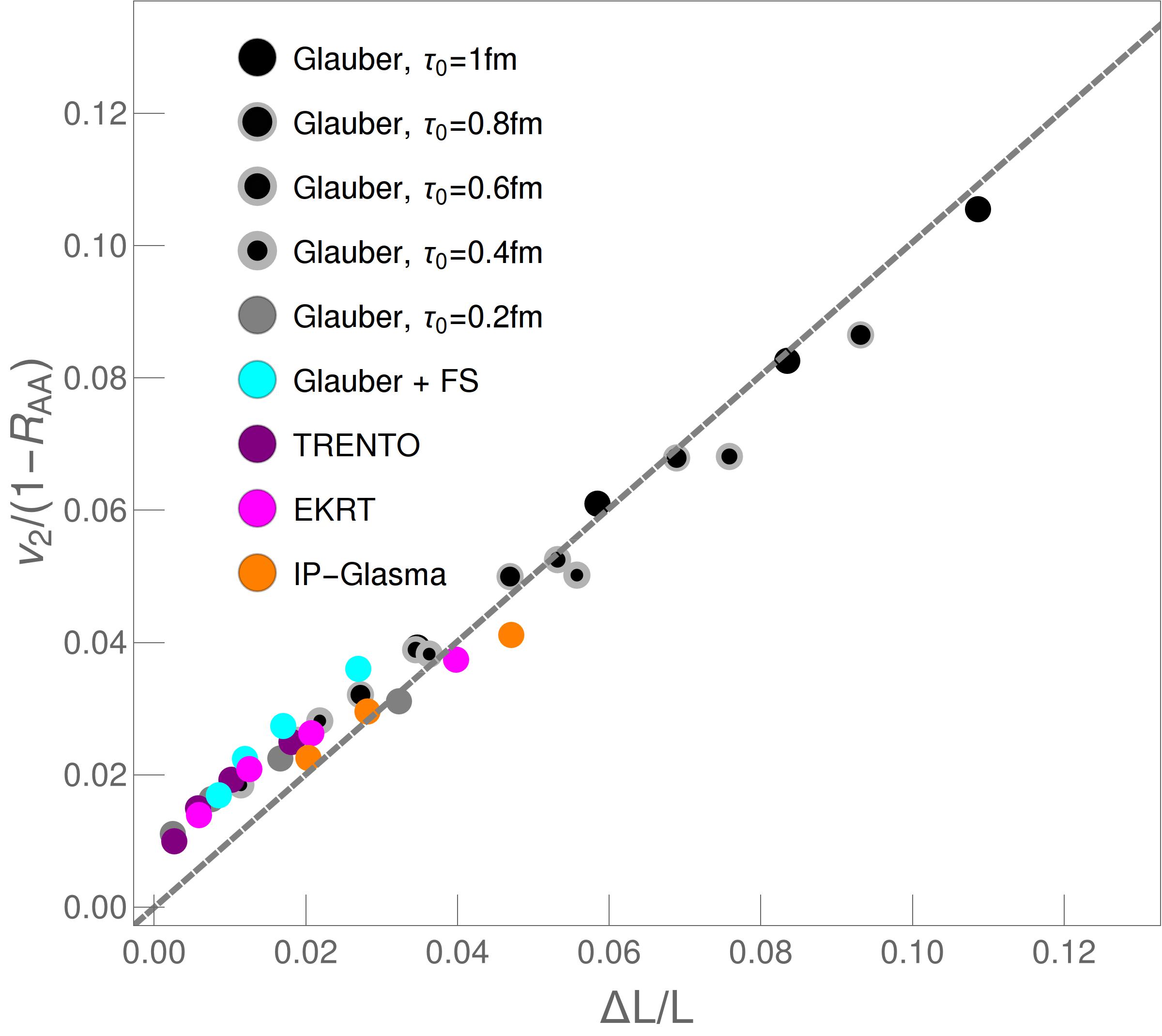
In Fig. 4 we have plotted the values of $v_{2}/(1-R_{AA})$ evaluated at 100 GeV for different evolution scenarios vs. the corresponding path-length anisotropies $\Delta L/\langle L\rangle$. Except for IP-Glasma, each scenario is presented with four points corresponding to the centrality classes 10-20%, 20-30%, 30-40%, 40-50%. We have omitted the 40-50% class of IP-Glasma since the average profile for this centrality class was not smooth enough to produce reliable $v_{2}$ and $R_{AA}$ results.

Figure 4 shows a surprisingly simple relation between $v_{2}/(1-R_{AA})$ and $\Delta L/\langle L\rangle$, where the dependence is linear with a slope of almost 1. The saturation value is therefore dominated by the geometry of the system, although at small values of $\Delta L/\langle L\rangle$ there is a deviation from the linear proportionality. It is worth noticing that here the values of $\Delta L/\langle L\rangle$ are much smaller than in our earlier 1D study shapeQGP . Also, even if the values of $\Delta L/\langle L\rangle$ are very different for different initializations, the initial anisotropies, $\epsilon_{2,2}$, are not so different. The general trend is that the earlier the transverse expansion begins (fluid dynamical or otherwise), the smaller the $\Delta L/\langle L\rangle$ in the same centrality class. The time it takes the parton to reach the edge of the system is almost independent of $\tau_{0}$, but small $\tau_{0}$ means that by the time the parton reaches the edge, the system has evolved longer, and the initial anisotropy has been diluted more. Thus, the earlier the expansion begins, the lower the $\Delta L$, and $\Delta L/\langle L\rangle$ depicts the mentioned sensitivity on the time when expansion begins.

Figure 5: The values of $v_{2}/(1-R_{AA})$ of charged hadrons as a function of the average jet-temperature anisotropy $\langle jT_{2}\rangle$ for various centrality classes and temperature profiles. The value of transverse momentum is fixed at $p_{\perp}=100$ GeV. The linear fit yields a slope of approximately 1.

$\Delta L/\langle L\rangle$ depends on the shape of the system, and how the shape evolves, but it is difficult to see how the evolution affects it. Thus, we wanted to see if it is possible to define a more direct measure of anisotropy, with an explicit dependence on time-evolution. After testing various generalizations of the conventional measure of the spatial anisotropy, $\epsilon_{m,n}$, we ended up evaluating the average of temperature cubed encountered by partons propagating with angle $\phi$ with respect to the reaction plane:

$$jT(\tau,\phi)\equiv\frac{\int\mathrm{d}x\mathrm{d}y\,T^{3}(x+\tau\cos\phi,y+\tau\sin\phi,\tau)\,n_{0}(x,y)}{\int\mathrm{d}x\mathrm{d}y\,n_{0}(x,y)},$$ (2)

where $n_{0}(x,y)$ is the density of the jets produced in the primary collisions, i.e., the density of the binary collisions. This distribution is not azimuthally symmetric, and we may evaluate its second Fourier coefficient:

$$jT_{2}(\tau)=\frac{\int\mathrm{d}x\mathrm{d}y\,n_{0}(x,y)\int\!\mathrm{d}\phi\cos 2\phi\,T^{3}(x+\tau\cos\phi,y+\tau\sin\phi,\tau)}{\int\mathrm{d}x\mathrm{d}y\,n_{0}(x,y)\int\!\mathrm{d}\phi\,T^{3}(x+\tau\cos\phi,y+\tau\sin\phi,\tau)}.$$ (3)

Moreover, a simple time-average of $jT_{2}$,

$$\langle jT_{2}\rangle=\frac{\int_{\tau_{0}}^{\tau_{\mathrm{cut}}}\mathrm{d}\tau\,jT_{2}(\tau)}{\tau_{\mathrm{cut}}-\tau_{0}},$$ (4)

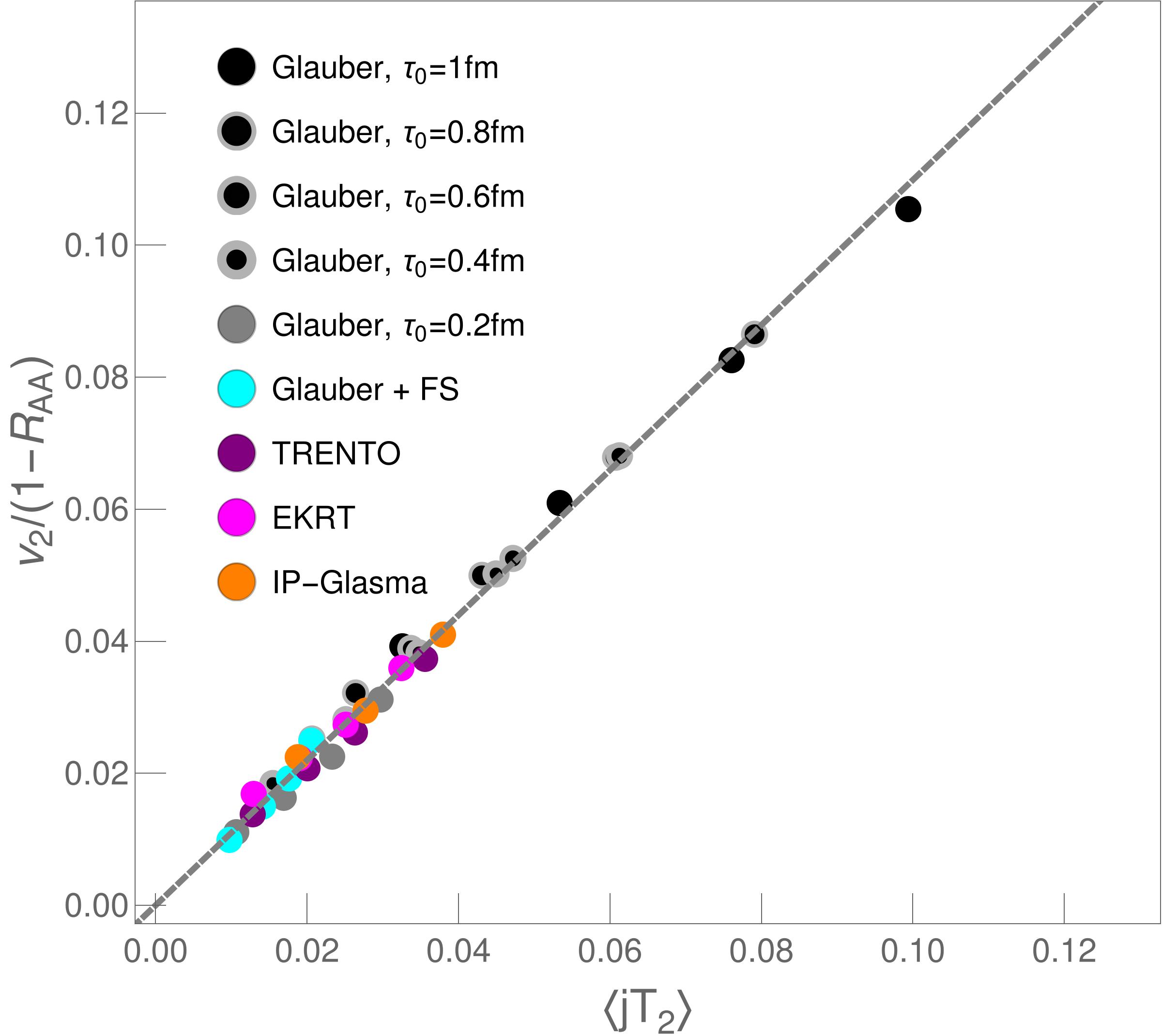
where $\tau_{\mathrm{cut}}$ is defined as the time when the center of the fireball has cooled down to critical temperature $T_{c}$, is directly proportional to the ratio $v_{2}/(1-R_{AA})$ as shown in Fig. 5.

We call this measure the average jet-temperature anisotropy of the system. When we evaluate the ratio of $v_{2}/(1-R_{AA})$ and $\langle jT_{2}\rangle$ in the $p_{\perp}$ range where the $v_{2}/(1-R_{AA})$ ratio has saturated for all models ($p_{\perp}>80$ GeV), and average over all the cases shown in Fig. 5 we obtain

$$\frac{v_{2}/(1-R_{AA})}{\langle jT_{2}\rangle}=1.1\pm 0.1.$$ (5)

Thus, $v_{2}/(1-R_{AA})$ at high-$p_{\perp}$ carries direct information of the system geometry, and its anisotropy. Since unity is within one standard deviation from the average, for practical purposes we use approximation $v_{2}/(1-R_{AA})=\langle jT_{2}\rangle$.

The above analysis was performed on charged hadrons. However, if $v_{2}/(1-R_{AA})$ indeed reflects the anisotropy $\langle jT_{2}\rangle$, then the Eq. (5) should be independent of flavor. Due to large mass, $R_{AA}$ and $v_{2}$ of heavy flavor particles depend on $p_{\perp}$ differently from charged hadrons’ $R_{AA}$ and $v_{2}$. To test whether the $v_{2}/(1-R_{AA})$ ratio of heavy flavor particles also saturates at high $p_{\perp}$, and whether Eq. (5) is valid for them, we performed the same analysis on $R_{AA}$ and $v_{2}$ of D and B mesons. We obtained that $v_{2}/(1-R_{AA})$ indeed saturates at $p_{\perp}>20$ GeV for B mesons and at $p_{\perp}>80$ GeV for D mesons, and that, after saturation, the Eq. (5) is robust for all types of flavor (results not shown). This further supports that $v_{2}/(1-R_{AA})$ at high-$p_{\perp}$ directly carries information on the medium property, as revealed through this extensive analysis.

Figure 6: Constraints to jet-temperature anisotropy ($\langle jT_{2}\rangle$, shown on y-axis) evaluated from high-$p_{\perp}>$ 20GeV $R_{AA}$ and $v_{2}$ experimental data using $\langle jT_{2}\rangle=v_{2}/(1-R_{AA})$ (see Eq. 5), for four different centrality regions (shown on x-axis): 10-20%, 20-30%, 30-40%, 40-50%. 5.02 TeV Pb+Pb ALICE ALICE_CH_RAA ; ALICE_CH_v2 (red triangles), CMS CMS_CH_RAA ; CMS_CH_v2 (blue squares) and ATLAS ATLAS_CH_RAA ; ATLAS_CH_v2 (green circles) data are used. For each centrality, the experimental constraints are compared with the average jet-temperature anisotropy $\langle jT_{2}\rangle$ for various evolution scenarios, indicated on the legend.

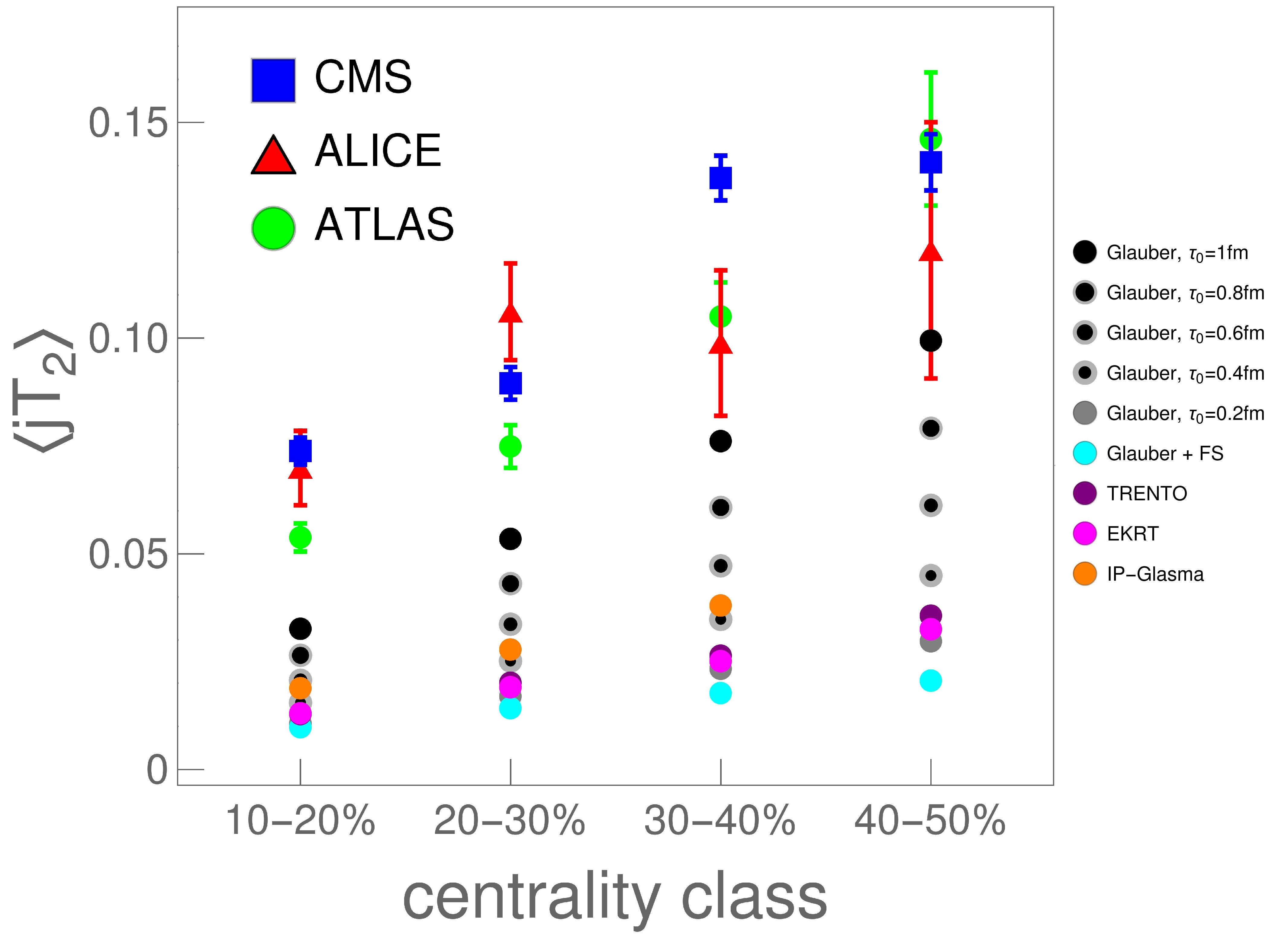
Finally, we evaluated the favored $\langle jT_{2}\rangle$ range from the experimentally measured $R_{AA}(p_{\perp})$ and $v_{2}(p_{\perp})$ for charged hadrons at different centralities. The $\langle jT_{2}\rangle$ values are obtained by fitting $v_{2}(p_{\perp})/(1-R_{AA}(p_{\perp}))$ experimental data shown in Fig. 3 with a constant function for $p_{\perp}>20$ GeV using MINUIT MINUIT package within ROOT ROOT code, taking uncertainties into account. The fitted ratio was then converted to $\langle jT_{2}\rangle$ by assuming their equality. As shown in Fig. 6, all three experiments lead to similar values of $\langle jT_{2}\rangle$, though the uncertainty is still large.

We also note that $\langle jT_{2}\rangle$ is a bulk-medium property, which can be directly evaluated from bulk-medium simulations through Eqs. (2)–(4), independently of high-$p_{\perp}$ data. Thus, experimental data can be used to restrict the value of this quantity. In Fig. 6, we see that none of the evolution scenarios tested in this manuscript is in good agreement with the experimental data (despite the above mentioned large uncertainty), i.e., lead to smaller jet-temperature anisotropy than experimentally favored. We thus show that jet-temperature anisotropy provides an important constraint on bulk-medium simulations, and that future bulk-medium calculations should be tuned to reproduce the experimentally constrained $\langle jT_{2}\rangle$ as well. Moreover, in the high-luminosity $3^{rd}$ run at the LHC, the error bars for $R_{AA}(p_{\perp})$ and $v_{2}(p_{\perp})$ are expected to be significantly reduced, which will subsequently lead to a notably better experimental constraint of $\langle jT_{2}\rangle$, also enabling better constraint on bulk-medium simulations.

IV Summary

In this study, we used our recently developed DREENA-A framework to explore how the temperature evolution of the QGP droplet influences high-$p_{\perp}$ $v_{2}/(1-R_{AA})$ predictions. The framework does not use any free parameter within the energy loss model and consequently allows to fully explore these profiles as the only input in the model. We showed that saturation in $v_{2}/(1-R_{AA})$, clearly seen in the experimental data, is robustly obtained for the comprehensive set of fluid-dynamical calculations covered in this study, as well as different types of flavor. We further revealed that this saturation value corresponds to a property of the system we defined as average jet-temperature anisotropy $\langle jT_{2}\rangle$. We also showed how to relate $\langle jT_{2}\rangle$ to experimental data, providing a new important constraint on bulk-medium simulations. None of the evolution scenarios that we tested here was in good agreement with experimentally inferred $\langle jT_{2}\rangle$ values, which argues that it is important to accordingly tune the bulk-medium simulations, particularly with the high-luminosity $3^{rd}$ run at the LHC. Our approach demonstrates the utility of the QGP tomography, i.e., the potential for extracting the bulk QGP properties jointly from low and high-$p_{\perp}$ data.

Acknowledgments: We thank Chun Shen and Harri Niemi for sharing their results with us. This work is supported by the European Research Council, grant ERC-2016-COG: 725741, and by the Ministry of Science and Technological Development of the Republic of Serbia. PH was also supported by the program Excellence Initiative Research University of the University of Wrocław of the Ministry of Education and Science.

References

- (1) M. Gyulassy and L. McLerran, Nucl. Phys. A 750, 30 (2005).
- (2) E.V. Shuryak, Nucl. Phys. A 750, 64 (2005).
- (3) C.V. Johnson and P. Steinberg, Phys. Today 63, 29 (2010).
- (4) B. Jacak and P. Steinberg, Phys. Today 63, 39 (2010).
- (5) J.C. Collins and M.J. Perry, Phys. Rev. Lett. 34, 1353 (1975).
- (6) G. Baym and S.A. Chin, Phys. Lett. B 62, 241 (1976).
- (7) M. Djordjevic, S. Stojku, M. Djordjevic, P. Huovinen, Phys. Rev. C 100, 031901 (2019).
- (8) J. D. Bjorken, Phys. Rev. D 27, 140 (1983).
- (9) D. Zigic, I. Salom, M. Djordjevic and M. Djordjevic, Phys. Lett. B 791, 236 (2019).
- (10) S. Acharya et al. [ALICE Collaboration], JHEP 1811, 013 (2018).
- (11) S. Acharya et al. [ALICE Collaboration], JHEP 1807, 103 (2018).
- (12) V. Khachatryan et al. [CMS Collaboration], JHEP 1704, 039 (2017).
- (13) A. M. Sirunyan et al. [CMS Collaboration], Phys. Lett. B 776, 195 (2018).
- (14) [ATLAS Collaboration], ATLAS-CONF-2017-012, (unpublished), https://cds.cern.ch/record/2244824.
- (15) M. Aaboud et al. [ATLAS Collaboration], Eur. Phys. J. C 78, 997 (2018).
- (16) E. Molnar, H. Holopainen, P. Huovinen and H. Niemi, Phys. Rev. C 90, 044904 (2014).
- (17) S. Stojku, J. Auvinen, M. Djordjevic, P. Huovinen and M. Djordjevic, arXiv:2008.08987 [nucl-th].
- (18) A. Bazavov et al. [HotQCD Collaboration], Phys. Rev. D 90, 094503 (2014).
- (19) P. Huovinen and P. Petreczky, Nucl. Phys. A 837, 26-53 (2010).
- (20) H. Niemi, K. J. Eskola and R. Paatelainen, Phys. Rev. C 93, 024907 (2016).
- (21) K. J. Eskola, K. Kajantie, P. V. Ruuskanen and K. Tuominen, Nucl. Phys. B 570, 379 (2000).
- (22) R. Paatelainen, K. J. Eskola, H. Holopainen and K. Tuominen, Phys. Rev. C 87, 044904 (2013).
- (23) R. Paatelainen, K. J. Eskola, H. Niemi and K. Tuominen, Phys. Lett. B 731, 126 (2014).
- (24) J. Auvinen, K. J. Eskola, P. Huovinen, H. Niemi, R. Paatelainen and P. Petreczky, Phys. Rev. C 102, 044911 (2020).
- (25) B. Schenke, P. Tribedy and R. Venugopalan, Phys. Rev. Lett. 108, 252301 (2012).
- (26) B. Schenke, P. Tribedy and R. Venugopalan, Phys. Rev. C 86, 034908 (2012).
- (27) E. Iancu, A. Leonidov and L. McLerran, arXiv:hep-ph/0202270.
- (28) E. Iancu and R. Venugopalan, in “Quark-Gluon Plasma 3”, pages 249–363, eds. R. C. Hwa and X.-N. Wang (World Scientific, Singapore, 2004) [arXiv:hep-ph/0303204].
- (29) F. Gelis, E. Iancu, J. Jalilian-Marian and R. Venugopalan, Ann. Rev. Nucl. Part. Sci. 60, 463 (2010).
- (30) T. Lappi, Int. J. Mod. Phys. E 20, 1 (2011).
- (31) B. Schenke, C. Shen and P. Tribedy, Phys. Rev. C 102, 044905 (2020)
- (32) C. Shen, private communication (2020).
- (33) B. Schenke, S. Jeon and C. Gale, Phys. Rev. C 82, 014903 (2010).
- (34) B. Schenke, S. Jeon and C. Gale, Phys. Rev. Lett. 106, 042301 (2011).
- (35) B. Schenke, S. Jeon and C. Gale, Phys. Rev. C 85, 024901 (2012).
- (36) A. Bazavov et al. [HotQCD], Phys. Rev. D 90, 094503 (2014).
- (37) J. S. Moreland and R. A. Soltz, Phys. Rev. C 93, 044913 (2016).
- (38) J. S. Moreland, J. E. Bernhard and S. A. Bass, Phys. Rev. C 92, 011901 (2015).
- (39) H. Song and U. W. Heinz, Phys. Rev. C 77, 064901 (2008).
- (40) J. E. Bernhard, arXiv:1804.06469 [nucl-th].
- (41) J. E. Bernhard, J. S. Moreland and S. A. Bass, Nature Phys. 15, no.11, 1113-1117 (2019).
- (42) D. Zigic, I. Salom, J. Auvinen, P. Huovinen and M. Djordjevic, arXiv:2110.01544 [nucl-th].
- (43) M. Djordjevic, Phys. Rev. C 80, 064909 (2009); M. Djordjevic and U. Heinz, Phys. Rev. Lett. 101, 022302 (2008).
- (44) M. Djordjevic, Phys. Rev. C 74, 064907 (2006).
- (45) B. Blagojevic and M. Djordjevic, J. Phys. G 42, 075105 (2015).
- (46) R. Baier, Y. Dokshitzer, A. Mueller, S. Peigne, and D. Schiff, Nucl. Phys. B 484, 265 (1997).
- (47) N. Armesto, C. A. Salgado, and U. A. Wiedemann, Phys. Rev. D 69, 114003 (2004).
- (48) M. Gyulassy, P. Lévai, and I. Vitev, Nucl. Phys. B 594, 371 (2001).
- (49) X. N. Wang and X. f. Guo, Nucl. Phys. A 696, 788-832 (2001).
- (50) J. I. Kapusta, Finite-Temperature Field Theory (Cambridge University Press, 1989).
- (51) M. Djordjevic and M. Gyulassy, Phys. Rev. C 68, 034914 (2003).
- (52) M. Djordjevic and M. Djordjevic, Phys. Lett. B 734, 286 (2014).
- (53) M. Djordjevic and M. Djordjevic, Phys. Lett. B 709, 229 (2012).
- (54) A. Peshier, hep-ph/0601119 (2006).
- (55) James, F.W. (1994). MINUIT Function Minimization and Error Analysis: Reference Manual Version 94.1.
- (56) R. Brun and F. Rademakers, Nucl. Inst. & Meth. in Phys. Res. A 389 (1997) 81-86.