Learning of Inter-Label Geometric Relationships Using Self-Supervised Learning: Application To Gleason Grade Segmentation

Abstract

Segmentation of Prostate Cancer (PCa) tissues from Gleason graded histopathology images is vital for accurate diagnosis. Although deep learning (DL) based segmentation methods achieve state-of-the-art accuracy, they rely on large datasets with manual annotations. We propose a method to synthesize for PCa histopathology images by learning the geometrical relationship between different disease labels using self-supervised learning. We use a weakly supervised segmentation approach that uses Gleason score to segment the diseased regions and the resulting segmentation map is used to train a Shape Restoration Network (ShaRe-Net) to predict missing mask segments in a self-supervised manner. Using DenseUNet as the backbone generator architecture we incorporate latent variable sampling to inject diversity in the image generation process and thus improve robustness. Experiments on multiple histopathology datasets demonstrate the superiority of our method over competing image synthesis methods for segmentation tasks. Ablation studies show the benefits of integrating geometry and diversity in generating high-quality images, and our self-supervised approach with limited class-labeled data achieves similar performance as fully supervised learning.

I Introduction

Prostate Cancer (PCa) is the sixth most common and second deadliest cancer among men worldwide. The most accurate PCa detection and staging is obtained from the analysis of stained biopsy tissue images. Each tissue region is assigned a Gleason grade between $1$ and $5$ (corresponding to the observed cellular patterns) and the final score is the sum of the most prominent and second most prominent patterns. Gleason scoring is subjective due to high level of heterogeneity leading to significant inter-observer and intra-observer variability [1, 2, 3, 4, 5, 6, 7, 8, 9, 10, 11, 12]. Computer-aided methods can potentially improve consistency, speed, accuracy, and reproducibility of diagnosis. Automated methods, especially state-of-the-art deep learning (DL) methods, require large image datasets for training. Owing to scarcity of such datasets, most approaches apply image augmentation to increase dataset size for network training.

Traditional augmentations such as image rotations or deformations do not fully represent the underlying data distribution of the training set, do not add qualitatively novel information, and are sensitive to parameter choices. Recent data augmentation methods of [13, 14, 15, 16, 17, 18, 19, 20, 21, 22, 23, 24, 25, 26] have used generative adversarial networks (GANs), [27, 28, 29, 30, 31, 32, 33, 34, 35, 36, 37], and show success for medical image classification. However, they have limited relevance for segmentation since they do not model geometric relation between different organs. Hence there is a need for augmentation methods that consider the geometric relation between different anatomical regions (labels) and generate realistic images for diseased and healthy cases.

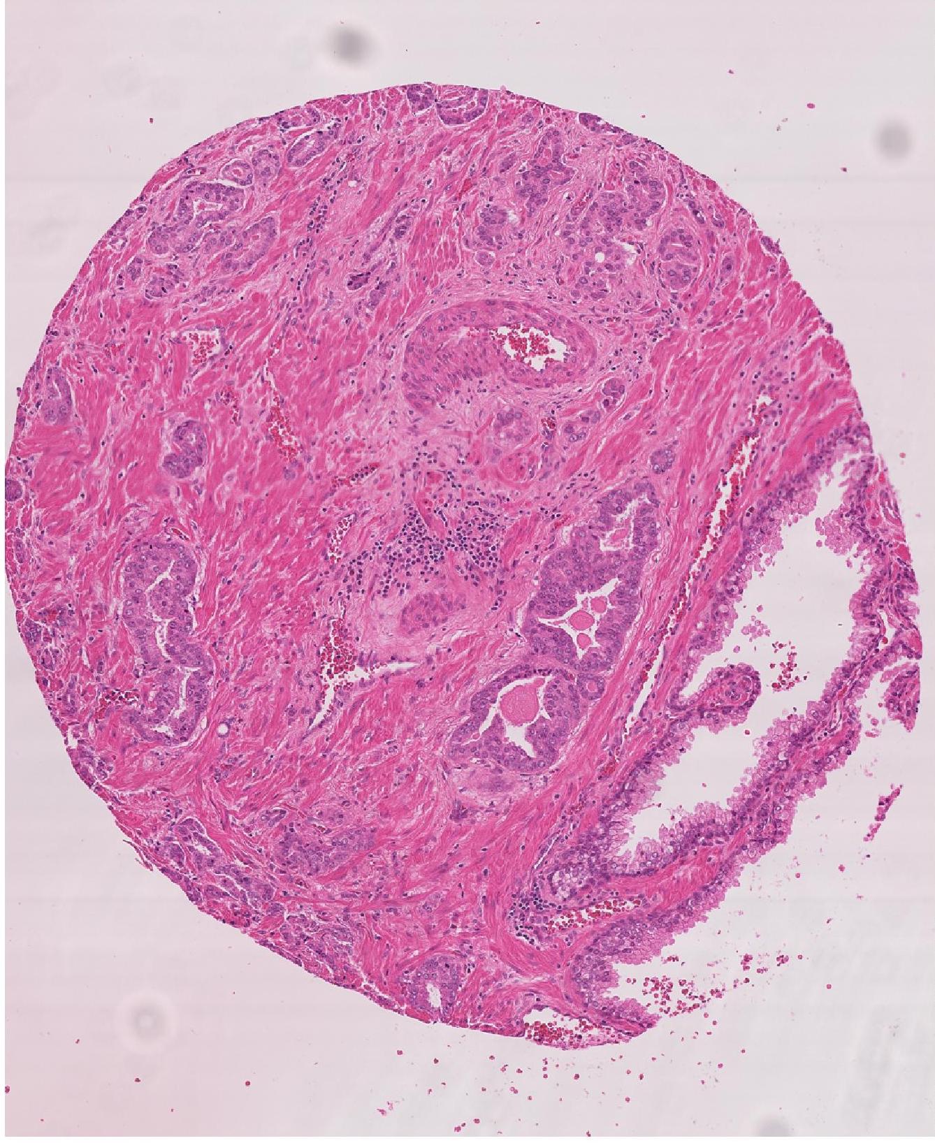
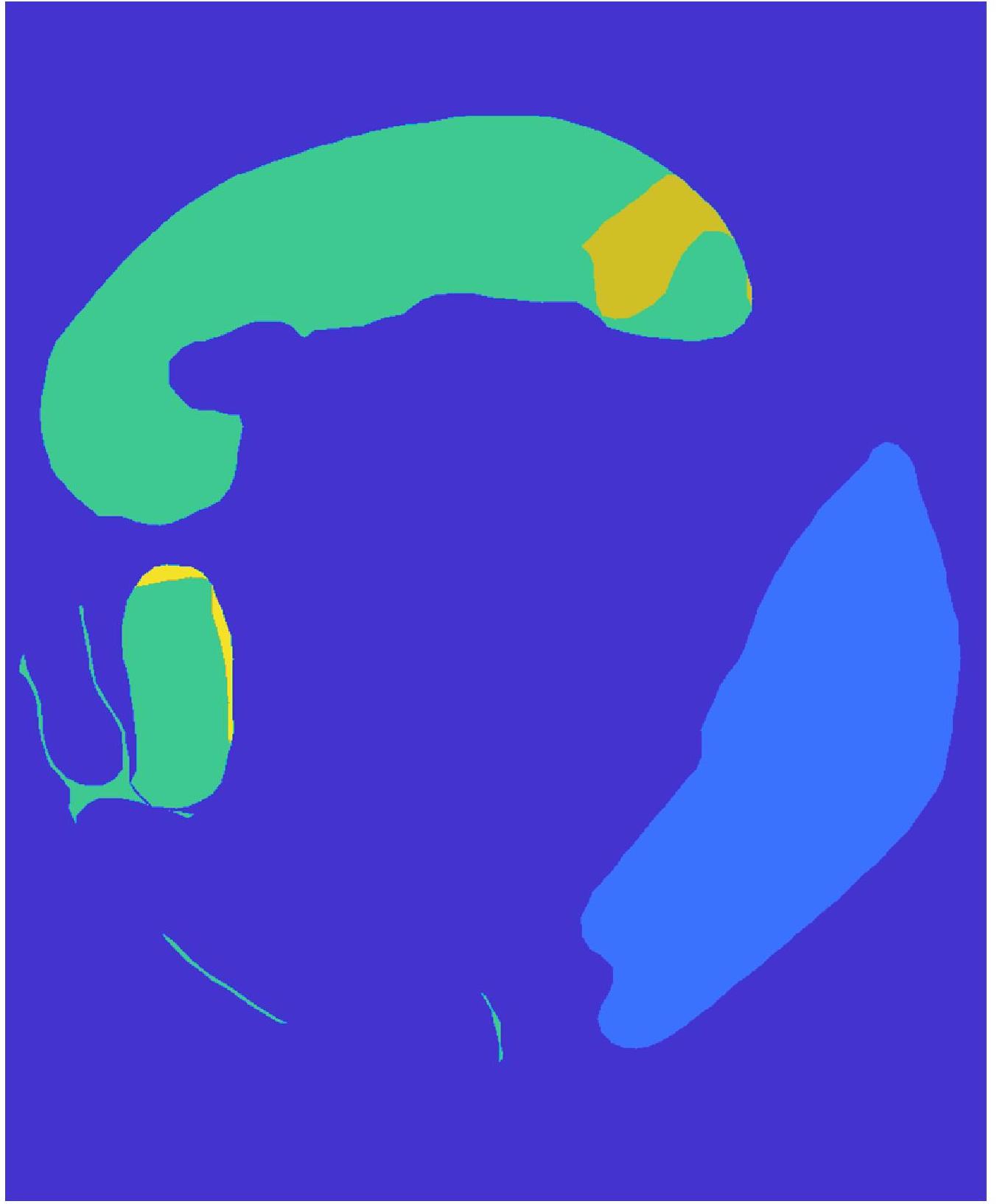
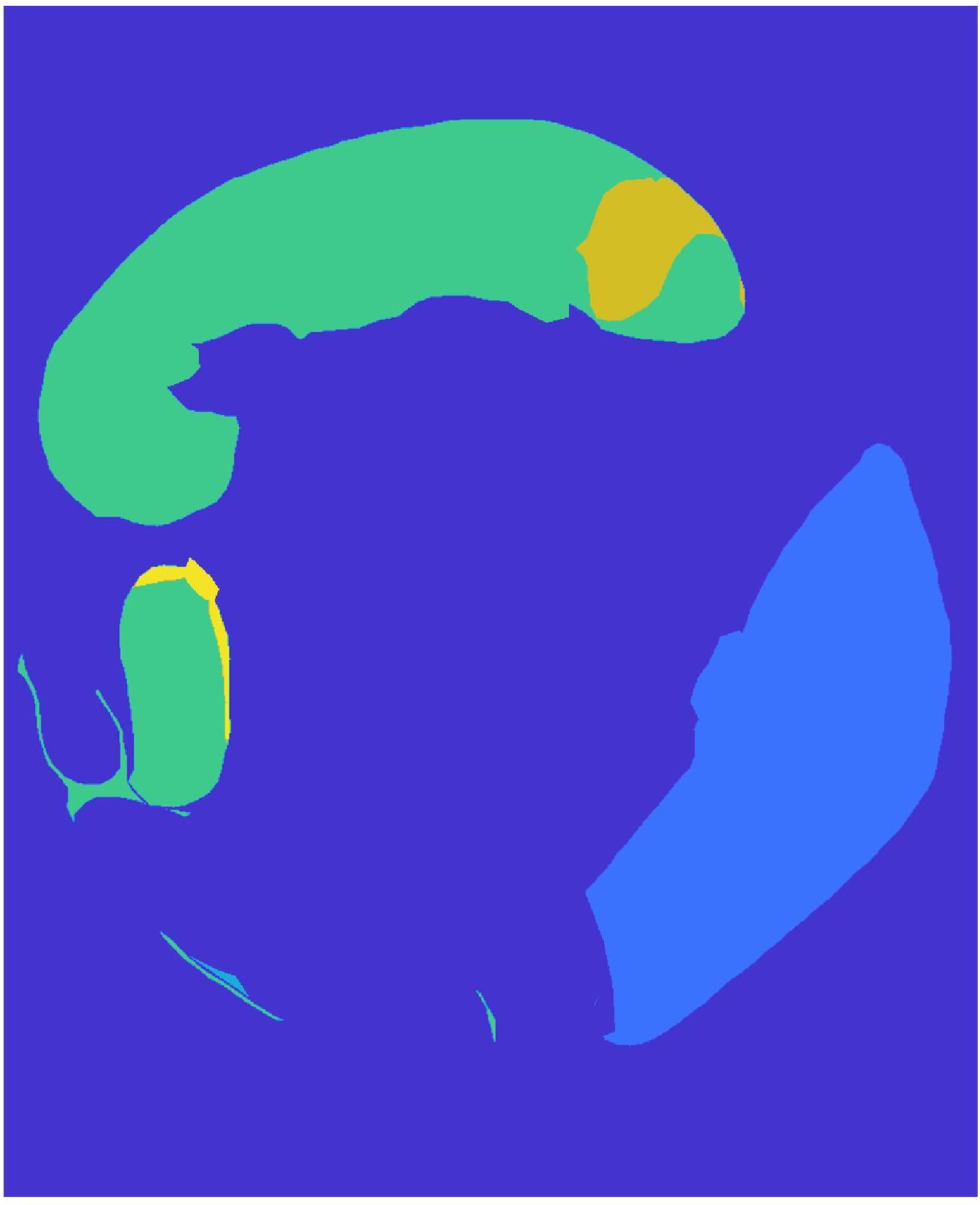
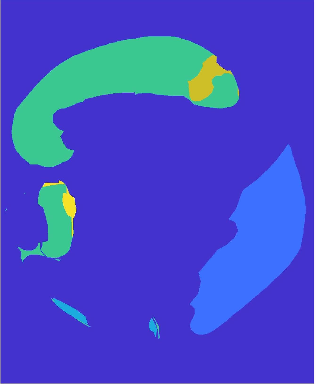
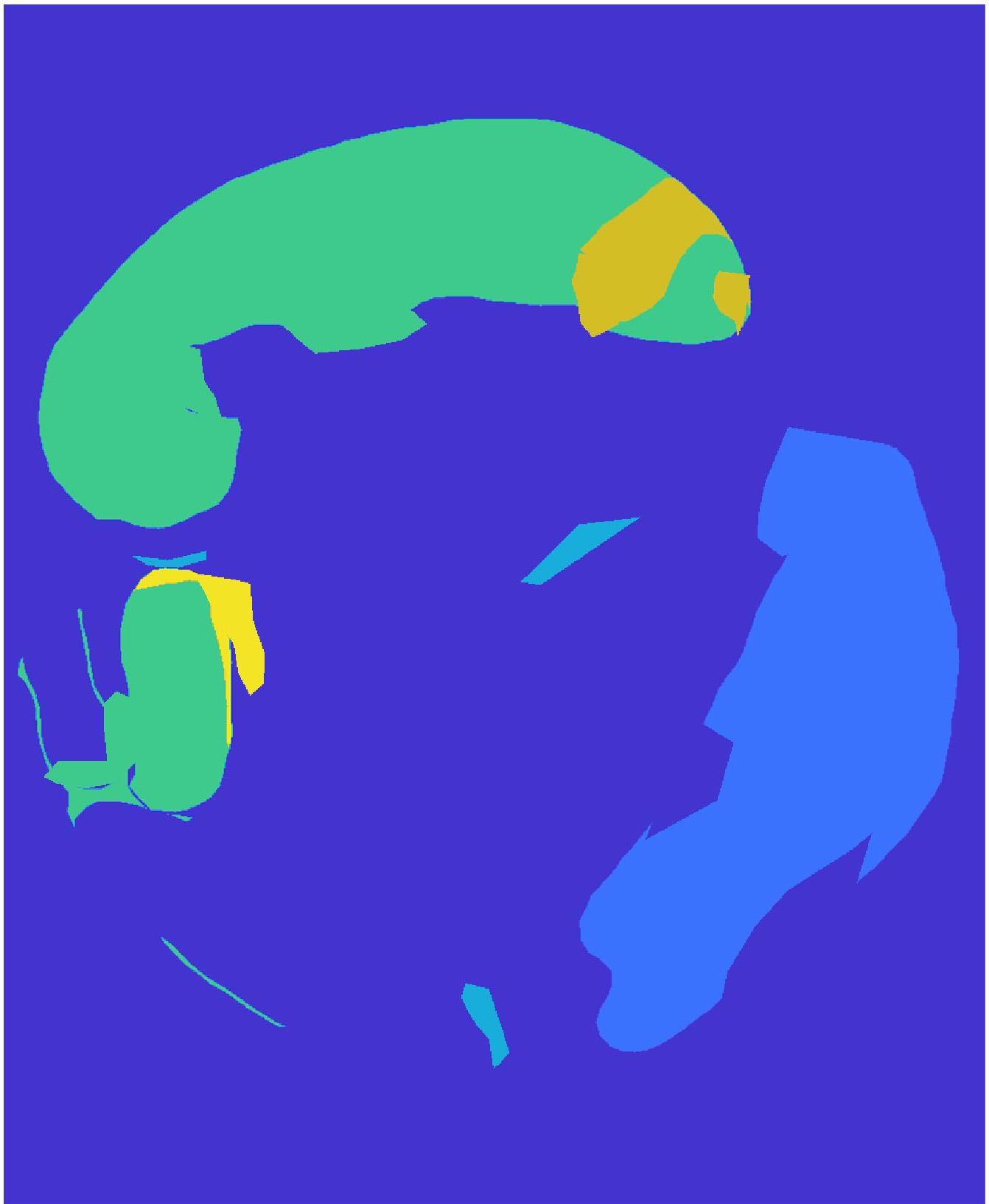
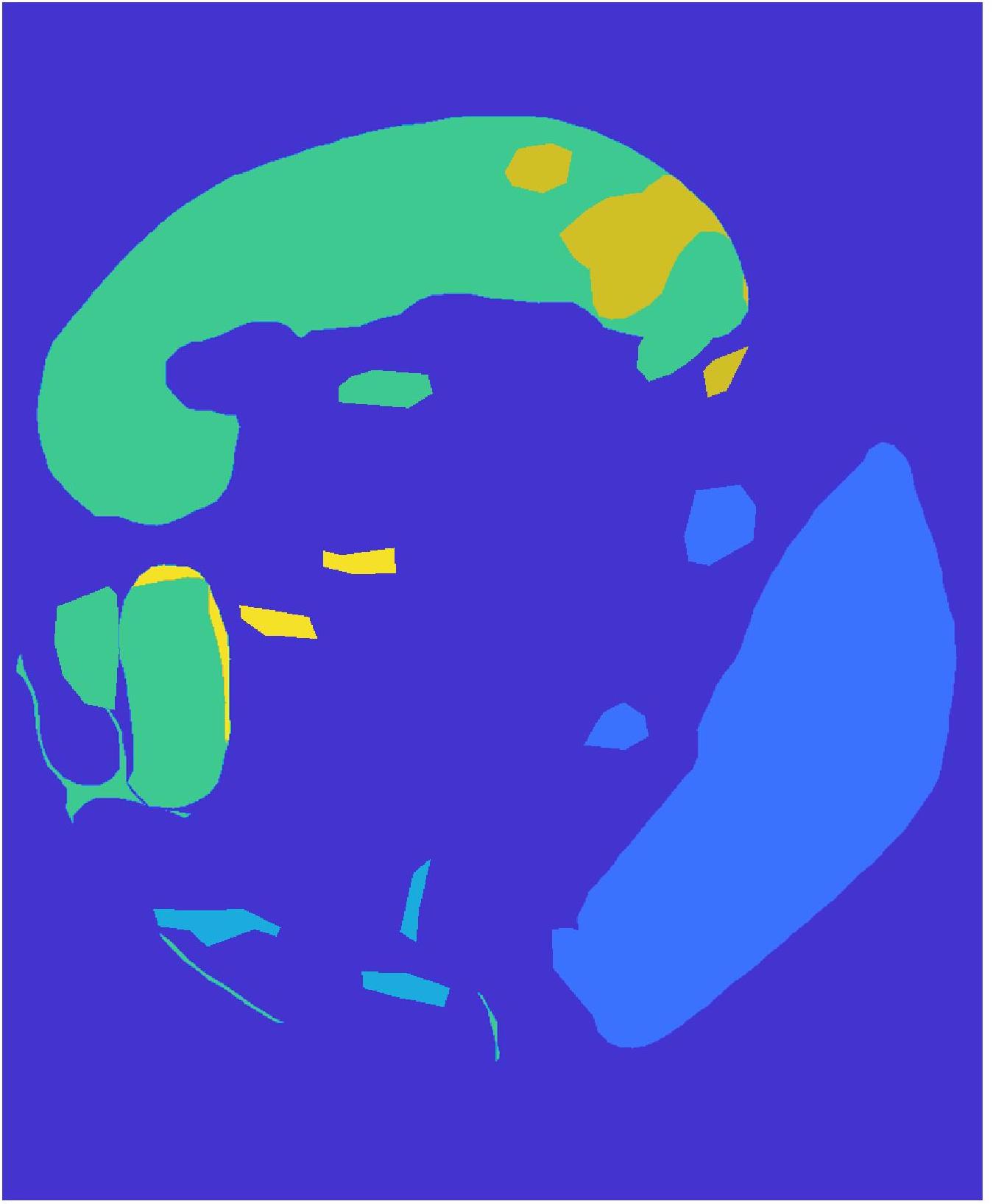
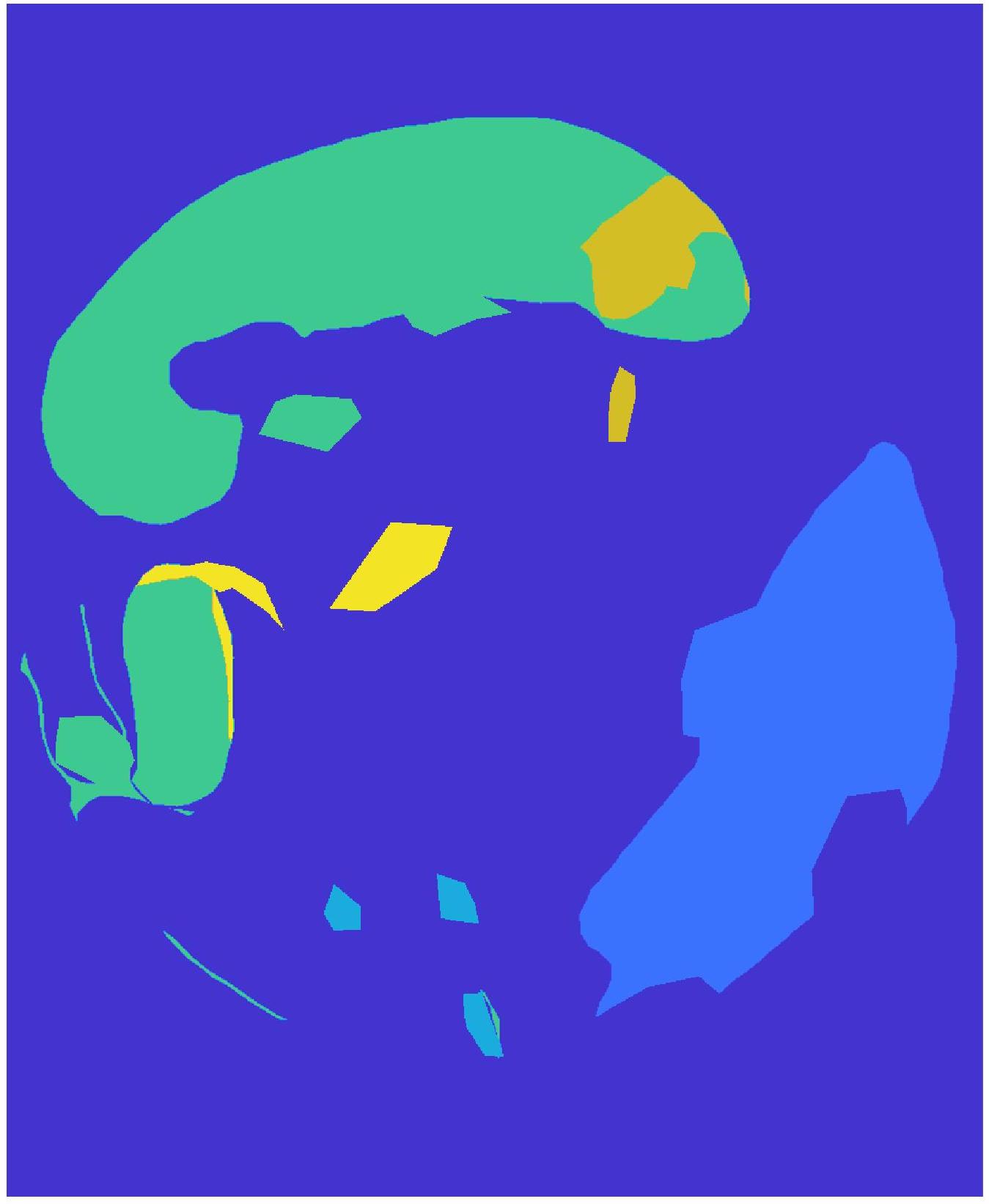
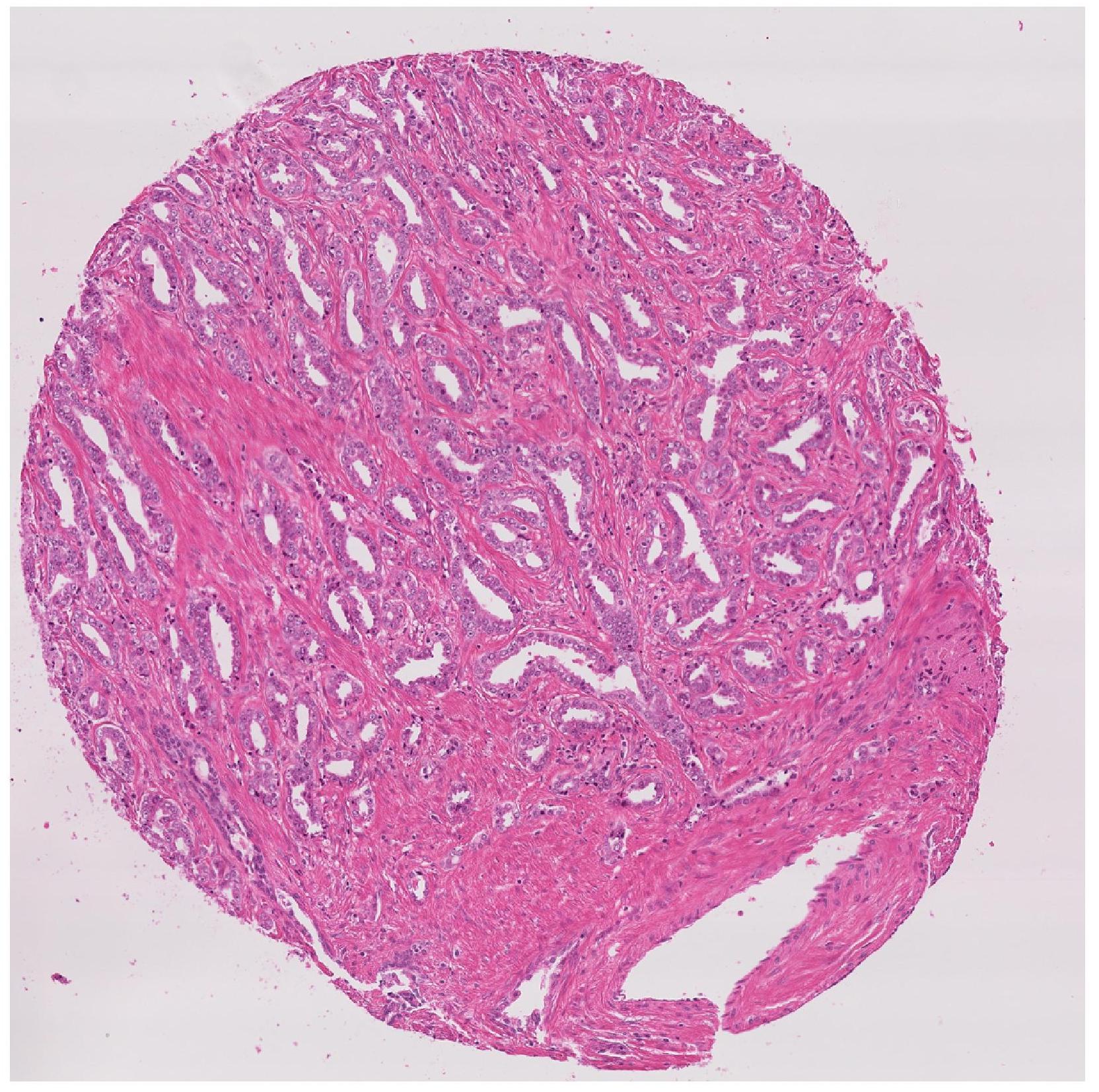
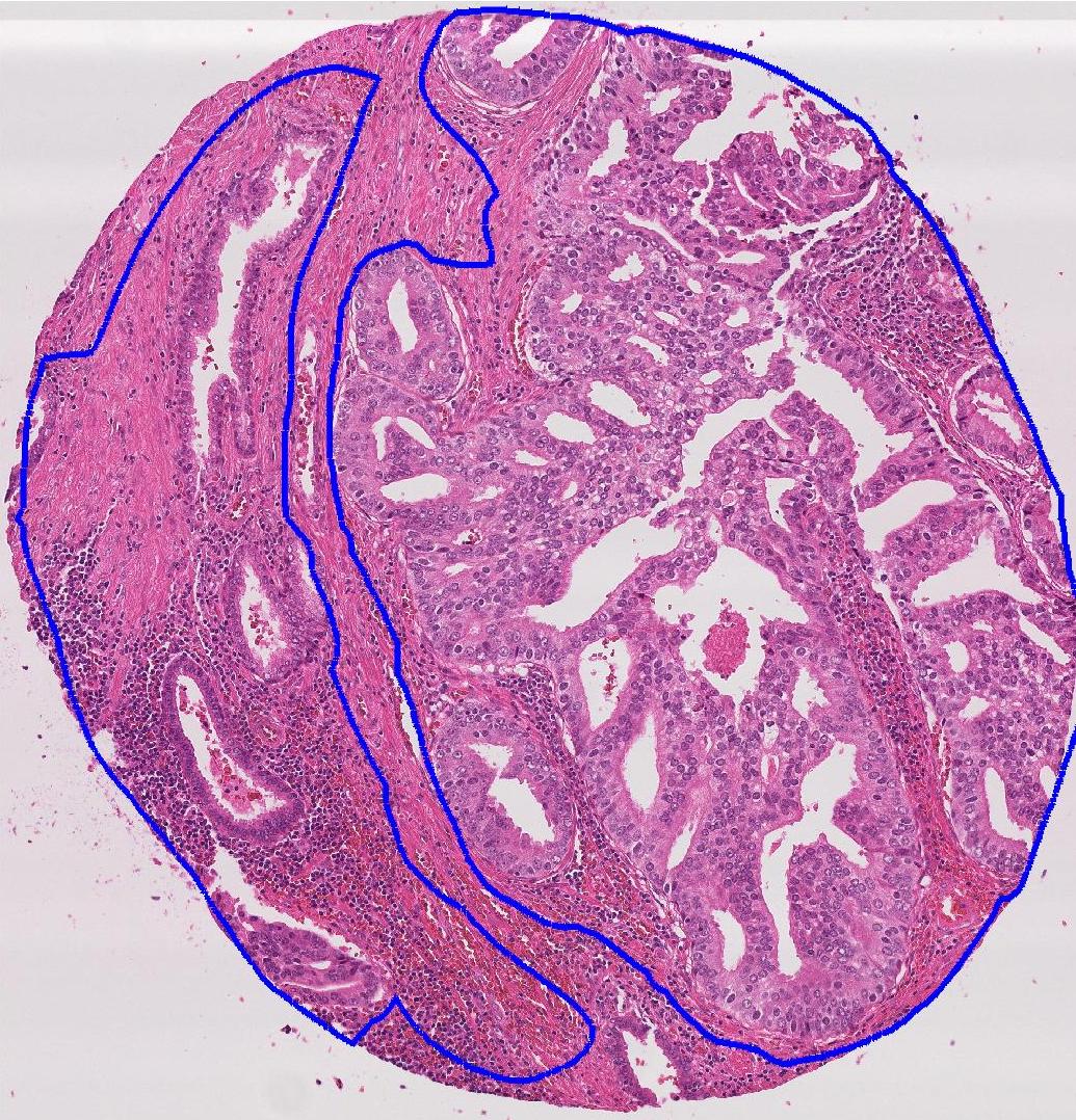
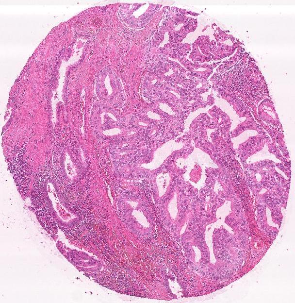
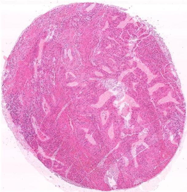
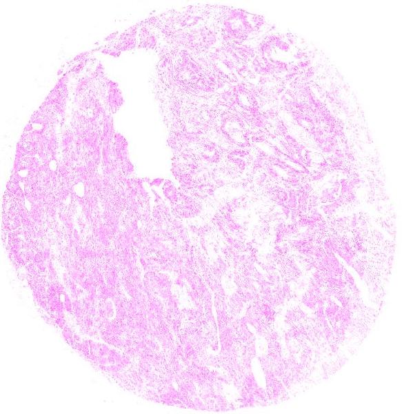
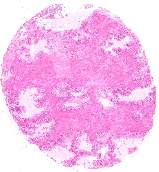
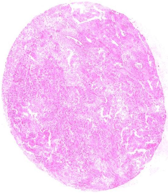
In this paper we propose a method to learn inter label geometric relationships using self-supervised learning. The learned model is used in a GAN framework to generate synthetic PCa histopathology images and used for segmentation of Gleason graded regions. Figure 1 shows example cases of synthetic images generated by our method and other competing techniques. A sample image generated by our approach is more realistic in appearance compared to the the base image, while other images have artifacts, noise, or distorted regions.

(a)	(b)	(c)	(d)	(e)	(f)

Figure 1: (a) Base image with Gleason graded regions shown as blue outline; Example of generated images using: (b) Our proposed $GeoGAN$ method; (c) [38]; (d) [39]; (e) $DAGAN$ method by [40]; (f) $cGAN$ method by [41].

I-A Our Contribution

We propose to generate more informative images by considering the intrinsic relationships between shape and geometry of anatomical structures. We present a Geometry-Aware Shape Generative Adversarial Network (GeoGAN) that learns to generate plausible images of different Gleason graded regions while preserving learned relationships between geometry and shape. Since annotating medical images is a time-consuming task, it is challenging to obtain manually annotated segmentation masks to model the geometrical relation between different image labels. To overcome this challenge, we propose to use a weakly supervised segmentation approach to generate labeled segmentation maps which are used to learn the geometric relationship between different pathological regions.

In an earlier version of our method, [42], we propose a GAN based approach for generating optical coherence tomography (OCT) images of retinal diseases. Apart from applying the method to histopathology images, our current work has the following additional novelties compared to [42]:

1. Weakly Supervised Segmentation: In [42] we used manual segmentation maps to learn inter-label geometrical relationships. However, that restricts the method to those datasets having manually annotated segmented maps, which are time-consuming to obtain. We introduce a novel weakly supervised semantic segmentation (WSSS) method that generates segmentation maps of histopathology images using the knowledge of disease grades. Different from [43]: 1) we use semi-supervised learning and label refinement in addition to clustering of autoencoder features; 2) we apply our approach to semantic segmentation while [43] use their method only for classification.

2. Self-Supervised Learning: We introduce a self-supervised learning based method to learn the inter-label geometrical relationships. In [42] we model this knowledge using a class conditional classifier. However, our experiments show that using the conditional classifier on the weakly supervised segmentation output affects the method’s robustness. Possible reasons are inherent errors in the segmentation output. Hence we use a pre-text task based self-supervised learning approach in this work to introduce greater robustness.

3. Uncertainty sampling: Previously in [42] we used a UNet based generator network for generating samples, and the uncertainty sampling was accordingly formulated. In our current work, we use Dense UNet [44], whose dense connections across previous layers facilitate more significant interaction between different levels of image representation.

II Related Work

Histopathology Image Analysis For Gleason Grading

Introduction of whole slide image (WSI) scanners has opened up the opportunity for computer-aided diagnosis (CAD) to aid pathologists and reduce inter-observer variability [45, 46, 47, 48, 49, 50, 51, 52, 53, 54, 55, 56]. To overcome issue of high dimensional WSI commonly used methods [57, 58, 42, 59, 60, 61, 62, 63, 64, 65, 66, 67] apply patch-level image classification or use sliding windows. Existing work on prostate biopsies use convolution neural networks [68, 69, 70, 71, 72, 73, 74, 75, 76, 77, 78, 79], semantic segmentation [80, 81, 82, 83, 84, 85, 86, 87, 88, 89, 90], feature-engineering [91, 92, 93, 94, 95, 96, 97, 98, 99, 100, 101, 102], and multiple instance learning for binary classification of clinical specimens [103, 104, 105, 106, 107, 108, 109, 110, 111, 112, 113, 114, 115, 116, 117, 118]. Nagpal et al.[119] developed a DL system to perform Gleason scoring and quantification of prostatectomy specimens including fine-grained measures of tumor grading.

Data Augmentation (DA)

Conventional augmentation approaches (such as rotation, scaling, etc.) do not add data diversity and are sensitive to parameter values [120, 121, 122, 123, 124, 125, 126, 127, 128, 129, 130, 131, 132, 133, 134], variation in image resolution, appearance, and quality [135, 136, 137, 138, 139, 140, 141, 142, 143, 144, 145, 146, 147, 148, 149]. Generative adversarial networks (GANs) have been very effective for data augmentation in few shot learning systems [40], chest xray images [41], cervical histopathological images [38], and to generate virtual histopathology images [39]. Zhao et al. [150] proposed a learning-based registration method to register images to an atlas, use the corresponding deformation field to deform a segmentation mask and obtain new data. GANs have also been used for generating synthetic retinal images in [151] and brain magnetic resonance images (MRI) in [13, 152], and generating higher strength MRI from their low strength acquisition counterparts [153]. However, there is no explicit attempt to model attributes such as shape variations that are important to capture different conditions across a population. [154, 155, 156, 157, 158, 159, 160, 161, 162, 163, 164, 165, 166, 167] augmented medical images with simulated anatomical changes but demonstrate inconsistent performance based on transformation functions and parameters.

Image Generation Using Uncertainty

Uncertainty based image generation has been realized using approximate Bayesian inference in scene understanding [168] while Lakshminarayanan et al. [169] generate different samples using an ensemble of $M$ networks and [170] use a single network with $M$ heads for image generation. Sohn et al. [171] use conditional variational autoencoders (cVAE) to model segmentation masks, while in probabilistic UNet [172], cVAE is combined with UNet [173] to generate multiple segmentation masks. Baumgartner et al. [174] generate images with greater diversity by injecting randomness at multiple levels. These approaches do not capture complex correlations between different labels

II-A Self-Supervised Learning

Self-supervised learning methods consist of two distinct approaches: 1) pretext tasks and 2) loss functions used for down-stream tasks. We use the pre-text approach to leverage the learned representation for generating synthetic images. In one of the first works on self-supervised learning in medical imaging, Jamaludin et al. [175] propose a siamese CNN to recognize patients’ MR scans and predict the level of vertebral bodies. Other works include surgical video re-colourisation as a pretext task for surgical instrument segmentation [176], rotation prediction for lung lobe segmentation and nodule detection [177], and disease bounding box localization for cardiac MR image segmentation [178]. Chen et al. [179] use context restoration as a pre-text for classification, segmentation, and disease localization in medical images. Self supervised learning has also been applied to histopathology images, using domain specific pretext tasks [180], semi-supervised histology classification [181] and cancer subtyping using visual dictionaries [182].

III Method

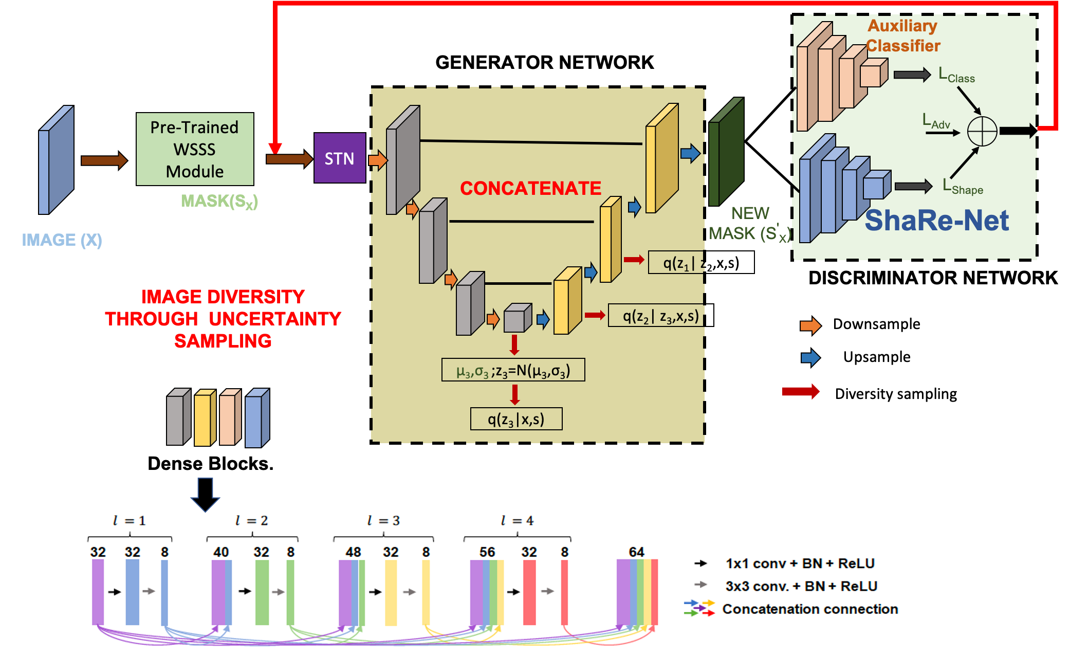
Our objective is to synthesize informative histopathology patches from a base image patch and train a segmentation model. Before the actual training of the synthetic image generator, the base image is segmented using a weakly supervised semantic segmentation step (the “Pre-Trained WSSS Module” in Figure 2). This gives us a base mask to learn inter-label geometric relationships. The first stage of synthetic image generation is a spatial transformation network (STN) that transforms the base mask with different location, scale, and orientation attributes. This initially transformed mask is input to the Dense-UNet based ‘Generator’ that injects diversity, and the discriminator ensures that the final generated mask is representative of the dataset. In addition to the adversarial loss ($L_{Adv}$) we incorporate losses from an auxiliary classifier ($L_{Class}$ to ensure the image has the desired label) and geometric relationship module ($L_{Shape}$ from ShaRe-Net).

Figure 2: Overview of the training stage of our method. The images ($X$) are input to the WSSS module which outputs corresponding segmentation masks ($S_{X}$) $S_{X}$ is input to a STN whose output is fed to the generator network. The DenseUNet based Generator network injects diversity at different levels through uncertainty sampling to generate a new mask $S_{X}^{{}^{\prime}}$. $S_{X}^{{}^{\prime}}$ is fed to the discriminator which evaluates its accuracy based on $L_{class}$, $L_{shape}$ and $L_{adv}$. The provided feedback is used for weight updates to obtain the final model. The architecture of each dense block is shown. Feature-maps from previous layers are concatenated together as the input to the following layers.

III-A Weakly Supervised Semantic Segmentation

To obtain pixel labels from image labels in a weakly supervised setting, we solve an instance-level classification problem with pixels as instances. In a weakly supervised setting, the image (bag) labels are known while the individual pixel (instance) labels need to be determined. A ‘normal’ bag indicates that all instances in the bag are labeled normal, while a ‘diseased’ bag indicates that at least one instance is diseased.

Gleason grades range from $1-5$ and describe resemblance of a biopsy to healthy tissue (lower score) or abnormal tissue (higher score). Most cancers score a grade of 3 or higher. Since prostate tumors are often made of cancerous cells with different grades, two grades are assigned for each patient. A primary grade describes the cells making up the largest area of the tumor, and a secondary grade describes the cells of the next largest area. A Gleason score of, for example, “5+4” indicates that the two most prominent patterns are Gleason grades $5$ and $4$. If the cancer is almost entirely made up of cells with the same score, the grade for that area is counted twice to calculate the total Gleason Score. However, there is also the possibility of the occurrence of other grades (such as $3$), which is not indicated in the bag label. To overcome this obstacle, we combine clustering with bag label information and semi-supervised learning to estimate the instance labels and then use these labels to train a multilabel segmentation network.

The work by Yamamoto et al. [43] investigate explainable features for predicting PCa recurrence where they employ autoencoder feature extraction and clustering. Our approach also uses autoencoder feature extraction followed by clustering to get a first estimate of labels of some pixels. However, not all pixel labels can be estimated by this approach for which we use additional steps such as: 1) semi-supervised learning for identifying labels of unlabeled samples; and 2) label refinement step for correcting the error of previous label prediction step.

The image pixels in our dataset can have any one of $5$ labels - background, benign, Gleason grades $3-5$. We denote these labels, respectively, as $[1,2,3,4,5]$. The background (label $1$) is identified by simple thresholding, and hence the challenge is to identify the instances of other labels. We rarely observe an image with a single label. Hence it is challenging to obtain examples of so-called normal labels (for example, benign). Therefore, we identify all possible subcategories and use knowledge of bag labels to assign labels to samples from all classes.

Figure 3: The workflow of weakly supervised segmentation. The image patch is processed through an autoencoder to extract latent features which are clustered using k-means. The two largest clusters are assigned labels of the Gleason grade and then input to a random forest-based semi-supervised classifier that outputs the unlabeled samples’ labels. The labeled samples are used to train a UNet++ network for obtaining the weakly supervised segmentation output.

III-A1 k-Means Clustering

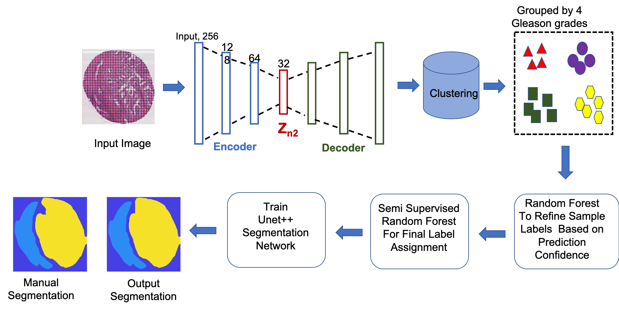
Most weak segmentation methods’ start with class activation maps (CAMs) to get the initial labels. and that requires a sufficiently high number of annotations. To use our method in a low resoruce setting we employ classical machine learning algorithms to identify sample labels. An image patch is split into $n\times n$ blocks ($n=16$). Each block is clustered using deep features extracted from an autoencoder trained to reconstruct the original $n\times n$ block. Note that neither the original mask nor the image are downsampled to lower resolutions.

Figure 3 shows the architecture of the autoencoder feature extractor. The $n\times n$ patch is converted into a $n^{2}$ vector and input to the autoencoder. The encoder stage has two hidden layers, followed by the latent representation of the original patch (denoted as $z_{n^{2}}$). The decoder layer reconstructs the original patch from $z_{n^{2}}$. The feature vectors $z_{n^{2}}$ from all instances of a bag are used as input to a k-means clustering algorithm that assigns each patch to one of $4$ clusters. At this stage, we only separate the samples into different clusters without knowing their actual label.

As stated previously, according to the Gleason grading criteria, the two Gleason grades correspond to the cells with the top two largest areas. The clusters with the highest and second highest number of samples correspond to those pixels/regions assigned the two Gleason scores for the particular image. Note that we group the features onto $4$ clusters for all images despite the fact that many images will have one or two distinct labels. This is due to two factors: 1) it reduces computation time as we do not have to find the optimal number of clusters for each image; 2) those samples which have been assigned labels according to the Gleason grade indicate high label confidence. For those images whose samples belong to, say, cluster $4$ and have been assigned cluster $1$, this discrepancy is corrected in the later stage of label refinement and semi-supervised learning.

Repeating the above steps for all images, we have a mix of ‘labeled’ and ‘unlabeled’ samples. ‘Labeled’ samples refer to those that have been assigned labels according to the image’s Gleason score (i.e., samples from the two largest clusters) and ‘unlabeled’ samples are from the other two clusters. The labeled samples have relatively high confidence and can be relied upon to train a robust and accurate classifier. Our next step is to remove those samples which may have been erroneously assigned to the ‘labeled’ clusters. For this purpose we train a supervised RF classifier to predict sample class using only the labeled samples, identify samples with low prediction confidence and remove them from the ‘labeled’ training set. RF is used because of its low memory requirement and ability to output confidence of predictions. The low confidence samples are then moved to the unlabeled set. We observe approximately $1.5\%$ samples to have low confidence, indicating the robust nature of our clustering approach.

III-A2 Semi Supervised Classification

We adopt the maximum margin approach to semi supervised random forests [183] to determine labels of unlabeled samples. Let $\textbf{g(x)}=[g_{1}(\textbf{x}),\cdots,g_{K}(\textbf{x})]^{T}$ be a multivalued function. g(x) is called a margin vector, if

$$\sum_{i=1}^{K}g_{i}(\textbf{x})=0$$ (1)

We can define the margin for the $i^{th}$ class as $g_{i}(\textbf{x})$ and the true margin as $g_{y}(\textbf{x})$. A loss function $\ell(g_{y}(\textbf{x}))$ is defined to be a margin maximizing loss if $\ell(g_{y}(\textbf{x}))\leq 0$ for all values of $g_{y}$. Therefore, an optimization based on this kind of loss functions will maximize the true margin. In the absence of a label there is no known true margin. Therefore the margin for unlabeled samples is defined as:

$$m_{u}(\textbf{x}_{u})=\max_{i\in\mathcal{Y}}g_{i}(x_{u})=0$$ (2)

where $\mathcal{Y}$ is the set of labels. Note that the predicted label for an unlabeled sample, $x_{u}$, is $C(x)=\arg\max_{i\in Y}g_{i}(x_{u})$.

Similar to the traditional regularization-based semi-supervised learning methods, we also regularize the loss for the labeled samples with a loss over the unlabeled samples. The overall loss function is

$$\mathcal{L}(g)=\frac{1}{\left|\mathcal{X}_{l}\right|}\sum_{(x,y)\in\mathcal{X}_{l}}\ell(g_{y}(x))+\frac{\alpha}{\left|\mathcal{X}_{u}\right|}\sum_{x\in\mathcal{X}_{u}}\ell(m_{u}(x_{u})),$$ (3)

where $\mathcal{X}_{l}$ denotes set of labeled samples, $\mathcal{X}_{u}$ denotes the unlabeled samples, and $\alpha=0.9$ defines the contribution rate of unlabeled samples. Training only on labeled data keeps the loss convex, while additional unlabeled data makes it non-convex. Hence Deterministic Annealing is used to obtain the global optimum and we refer to [183] for further details. The output of this step is a label for each instance ($n\times n$ block)

III-A3 Segmentation Using Standard Network

The assigned labels are mapped back to the $n\times n$ patches to obtain a segmentation map. Using these segmentation maps as the ground truth, we train a UNet++ network [184] to predict the segmentation labels of a new image. The UNet++ network has redesigned skip connections, and the loss function as defined in [184] is a combination of binary cross-entropy and Dice loss,

$$L(Y,\hat{Y})=-\frac{1}{N}\sum_{b=1}^{N}\left(\frac{1}{2}\cdot Y_{b}\cdot\log\hat{Y_{b}}+\frac{2Y_{b}\cdot\hat{Y_{b}}}{Y_{b}+\hat{Y_{b}}}\right)$$ (4)

where $\hat{Y_{b}},Y_{b}$ denote the flattened predicted probabilities and the ground truths of $b^{th}$ image respectively, and $N$ indicates the batch size.

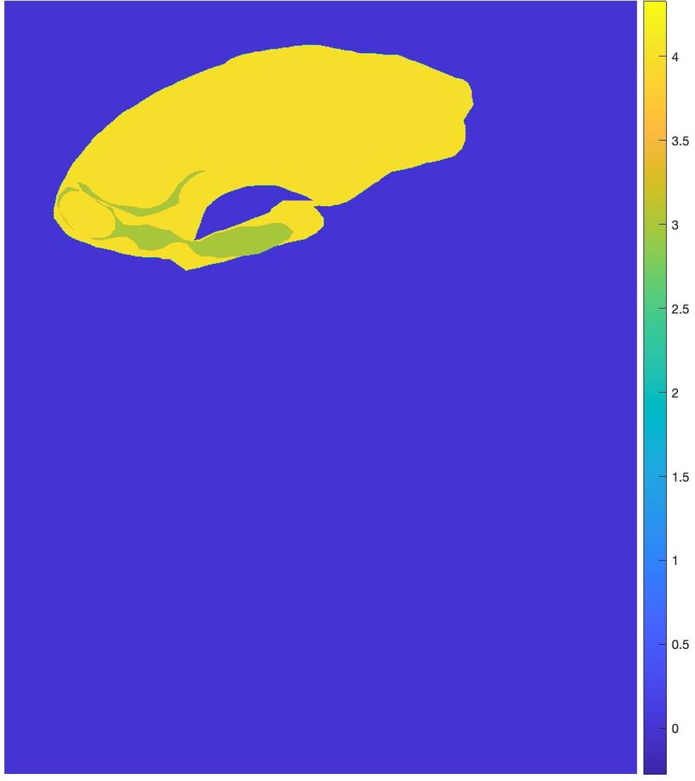
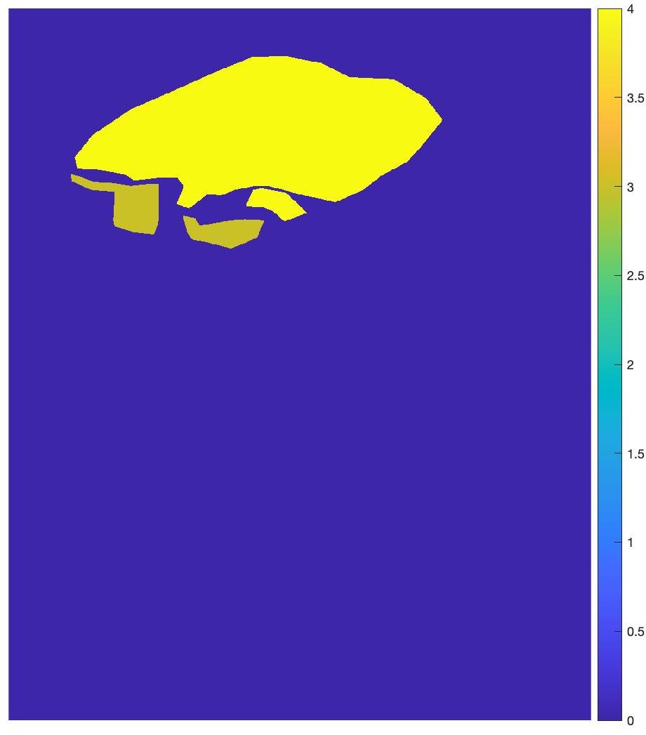
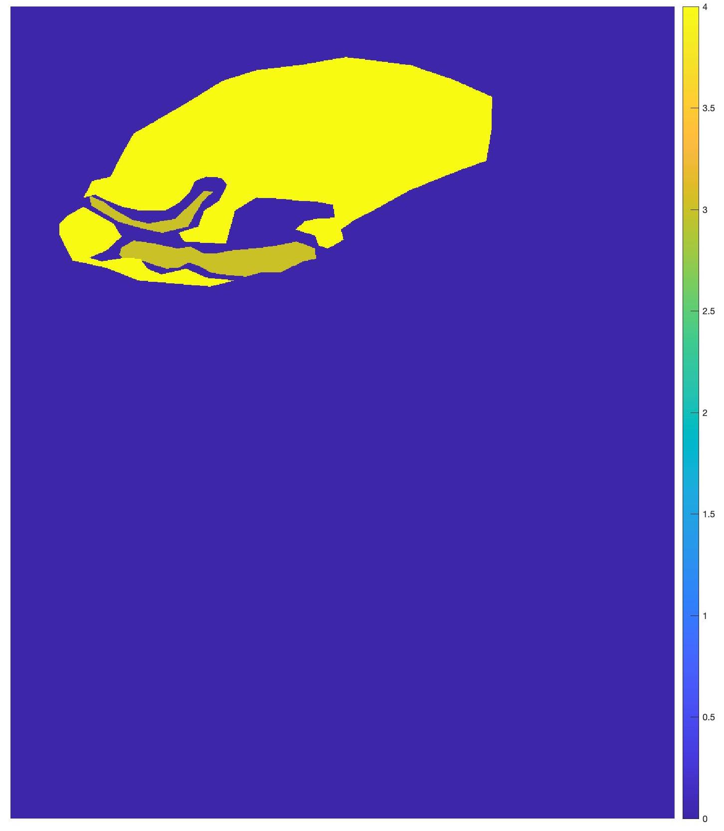
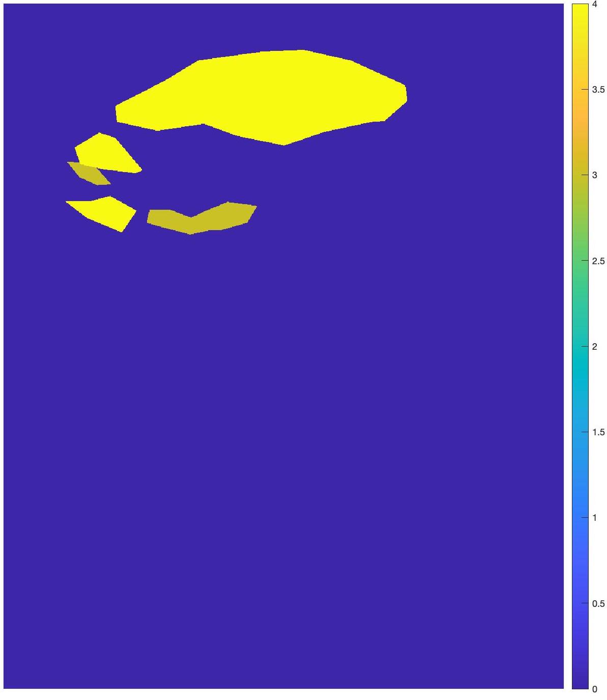
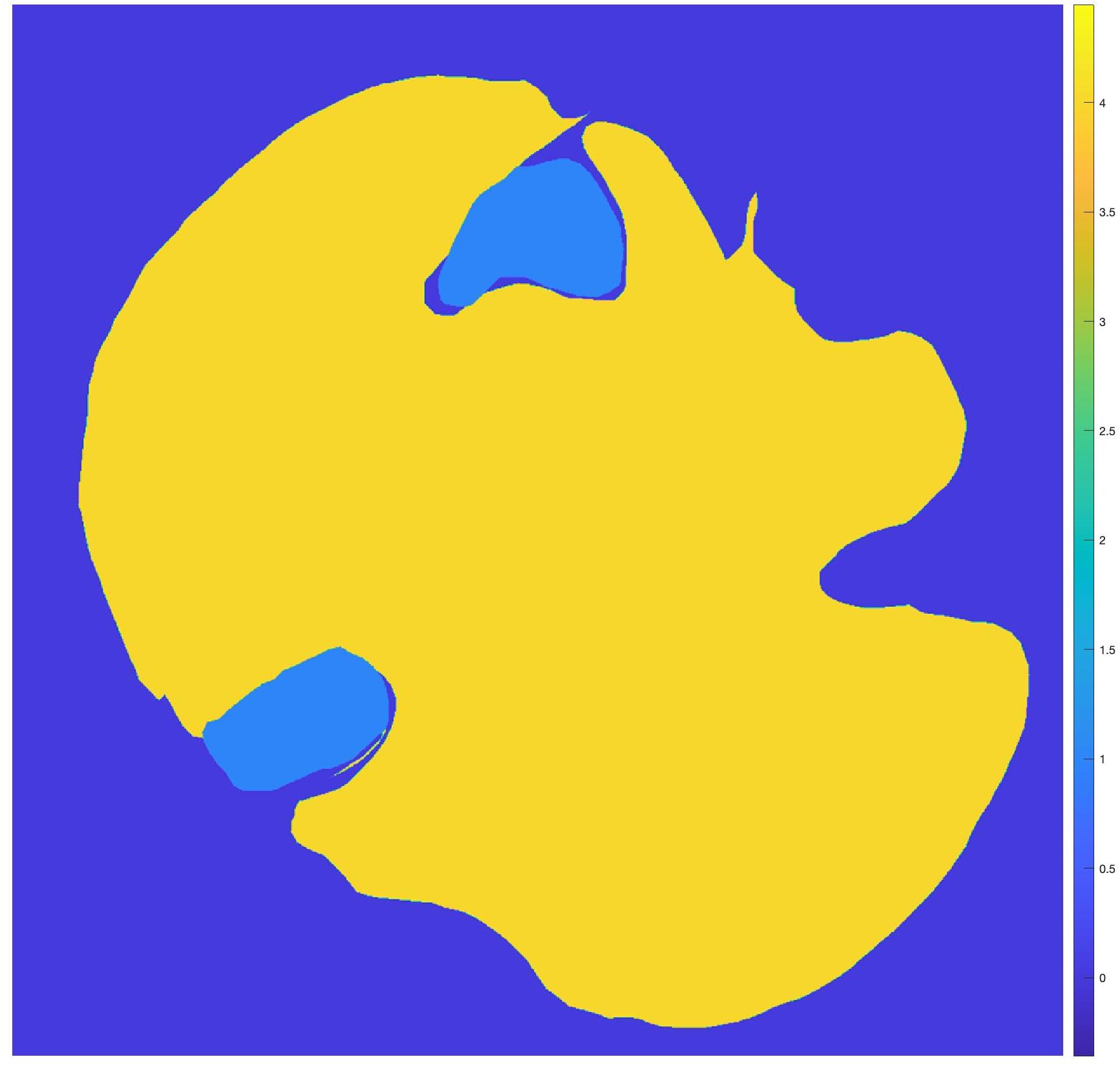
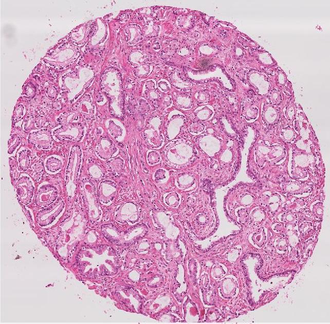
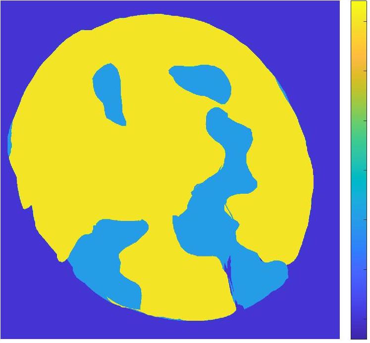
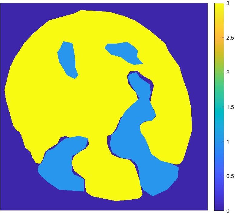
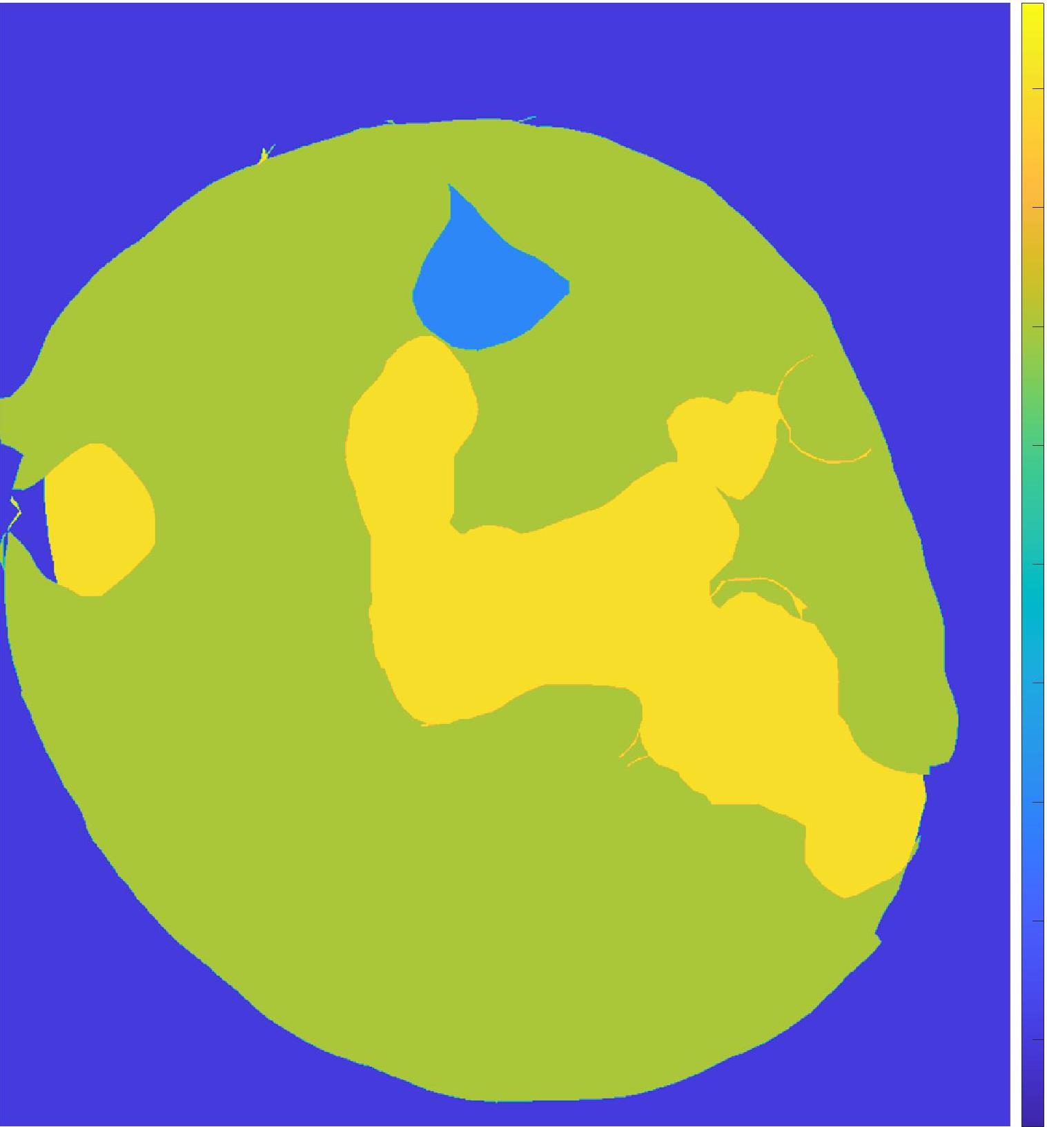
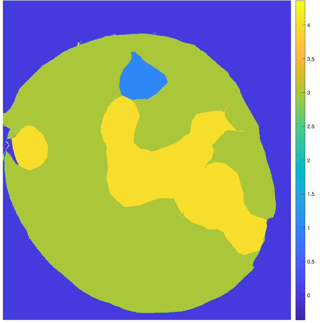
Ground truth maps obtained from the semi-supervised learning step has labels for each $n\times n$ block. Consequently, there will be cases where a pixel outside the actual structure of interest shares its label since it is part of the $n\times n$ block. This erroneous labeling is referred as label noise. Our experimental results show that the UNet++ network is more robust to such label noise than the conventional UNet. Figure 4 shows comparative results of using UNet and UNet++ in obtaining the weak segmentation map. UNet++ proves to be more robust to initial label noise. Figure 5 shows example images, their corresponding expert annotated manual segmentation maps, and the maps obtained using our method. A very high degree of agreement exists between weak supervision generated maps and the ground truth, with a Dice Metric of $0.962$ validating this observation. Without the label refinement step we obtain a Dice Metric of $0.941$, highlighting its contribution in improving segmentation performance. Using UNet we obtain a Dice metric of $0.930$ and $0.907$ (without label refinement), which indicates superior capacity of UNet++ to overcome label noise. Thus we repose high confidence in the weakly supervised generated label maps as representing the correct labels and are reliable enough to model inter-label geometric relationship (as described in the next step).

(a)	(b)	(c)	(d)

Figure 4: Demonstration of UNet++’s robustness to noisy labels. (a) manual ground truth segmentation label map; (b) initial noisy label map before refinement; (c) final label map generated by our weakly-supervised approach using UNet++; (d) label map generated using UNet. The color bar indicates the corresponding labels.

(a)	(b)	(c)

Figure 5: Results for weakly supervised segmentation compared to ground-truth maps. (a) original histopathology image; (b) manual ground truth segmentation label map; (c) label map generated by our weakly-supervised approach. The color bar indicates the corresponding labels.

III-B Geometry Aware Shape Generation

Let us denote an input image as $x$, the corresponding weakly supervised segmentation masks as $s_{x}$ and its label (Gleason score) as $l_{x}$. Our method learns to generate a new segmentation map from the base mask. The first stage is a spatial transformer network (STN) [185] that transforms the base mask with different attributes of location, scale and orientation. The transformations used to obtain new segmentation mask $s_{x}^{{}^{\prime}}$ are applied to $x$ to get corresponding transformed image $x^{{}^{\prime}}$. Since the primary aim of our approach is to learn contours and other shape specific information of anatomical regions, a modified DenseUNet architecture as the generator network effectively captures hierarchical shape information and easily introduces diversity at multiple levels of image generation.

The generator $\textbf{G}_{g}$ takes input $\textbf{s}_{x}$ and a desired label vector of output mask $c_{g}$ to output an affine transformation matrix A via a STN, i.e., $\textbf{G}_{g}$($\textbf{s}_{x},c_{g})=\textbf{A}$. A is used to generate $s_{x}^{{}^{\prime}}$ and $x^{{}^{\prime}}$. The discriminator $\textbf{D}_{class}$ determines whether output image preserves the desired label $c_{g}$ or not. The discriminator $\textbf{D}_{g}$ is tasked with ensuring that the generated masks are realistic. Let the minimax criteria between $\textbf{G}_{g}$ and $\textbf{D}_{g}$ be $\min_{\textbf{G}_{g}}\max_{\textbf{D}_{g}}\textbf{L}_{g}(\textbf{G}_{g},\textbf{D}_{g})$. The loss function $\textbf{L}_{g}$ is,

$$L_{g}=L_{adv}+\lambda_{1}{L}_{class}+\lambda_{2}{L}_{shape}$$ (5)

where 1) $\textbf{L}_{adv}$ is an adversarial loss to ensure $\textbf{G}_{g}$ outputs realistic deformations; 2) $\textbf{L}_{class}$ ensures generated image has same label as $x$ and preserves it’s Gleason grade; and 3) $\textbf{L}_{shape}$ ensures new masks have realistic shapes. $\lambda_{1}=0.95,\lambda_{2}=1$ balance each term’s contribution.

Adversarial loss- $\textbf{L}_{adv}(\textbf{G}_{g},\textbf{D}_{g})$

The STN outputs $\widetilde{A}$, a prediction for A conditioned on $\textbf{s}_{x}$, and a new semantic map $\textbf{s}_{x}\oplus\widetilde{A}(\textbf{s}_{x})$ is generated. $\textbf{L}_{adv}$ is defined as:

$$\begin{split}L_{adv}(G_{g},D_{g})=\mathbb{E}_{x}\left[\log D_{g}(\textbf{s}_{x}\oplus\widetilde{A}(\textbf{s}_{x}))\right]\\ +\mathbb{E}_{\textbf{s}_{x}}\left[\log(1-D_{g}(\textbf{s}_{x}\oplus\widetilde{A}(\textbf{s}_{x})))\right],\end{split}$$ (6)

Classification Loss- $\textbf{L}_{class}$

The affine transformation $\widetilde{A}$ is applied to the base image x to obtain the generated image $\textbf{x}^{{}^{\prime}}$. We add an auxiliary classifier (to ensure the output image has the desired label) when optimizing both $\textbf{G}_{g}$ and $\textbf{D}_{g}$ and define the classification loss as,

$$L_{class}=\mathbb{E}_{\textbf{x}^{{}^{\prime}},c_{g}}[-\log D_{class}(c_{g}|x^{\prime})],$$ (7)

where the term $D_{class}(c_{g}|x^{\prime})$ represents a probability distribution over classification labels computed by $D$.

Shape Loss-$\textbf{L}_{shape}$

Self Supervised Modeling of Inter-Label Geometric Relationships

We propose a novel approach to model the relationship between different anatomical labels. In [42] we achieve this by training a conditional classifier to output the label of an image region given another labeled region. However we find that use of a self-supervised learning based approach is much more effective in learning contextual information than our previous approach. Here we describe our novel approach in modeling the inter-label relationship.

Given a dataset of masks $S=\{s_{1},s_{2},\cdots,s_{N}\}$ consisting of N label masks, a new dataset $\hat{S}=f(S)$ is generated, where $f$ is a function altering the original label maps by arbitrarily masking labeled regions or swapping patches. A CNN is trained to predict the intensity values of the altered pixels. Here the intensity values correspond to the mask’s Gleason labels. The task here is to reconstruct the masks when part of it has been altered. By learning to predict the missing labels the network implicitly learns the geometrical relationship between different anatomical labels (Gleason grades).

We train an Encoder-Decoder style network similar to UNet where the input is the altered mask and the output is the original mask, and use a $L_{2}$ loss term. We call this network as the Shape Restoration Network (ShaRe-Net). To compute $L_{shape}$ we obtain the feature maps of the generated mask ($SN(G_{g}(\textbf{s}_{x}))$ and original mask $SN(\textbf{s}_{x})$ using all layers of ShaRe-Net, and calculate the mean square error values between them.

$$L_{shape}=\frac{1}{N}\sum_{i}^{N}\left(SN(\textbf{s}_{x})-SN(G_{g}(\textbf{s}_{x}))\right)^{2}$$ (8)

$SN(\cdot)$ denotes the input processed through ShaRe-Net.

III-C Sample Diversity From Uncertainty Sampling

Our approach based on uncertainty sampling is inspired from [174]. However we also introduce the novelty of using a Dense UNet architecture [44] instead of UNet. This allows us to reuse information from previous layers which introduces complementary information across layers. This enables the generation step to factor in the dependence across different levels of shape abstraction.

The generated mask $s_{x}^{\prime}$ is obtained by fusing $L$ levels of the generator $G_{g}$ (as shown in Figure 2), each of which is associated with a latent variable $z_{l}$. We use probabilistic uncertainty sampling to model conditional distribution of segmentation masks and use separate latent variables at multi-resolutions to factor inherent uncertainties. The hierarchical approach introduces diversity at different stages and influences different features (e.g., low level features at the early layers and abstract features in the later layers). Denoting the generated mask as $s$ for simplicity, we obtain conditional distribution $p(s|x)$ for $L$ latent levels as:

$$\begin{split}p(s|x)=\int p(s|z_{1},\cdots,z_{L})p(z_{1}|z_{2},x)\cdots\\ p(z_{L-1}|z_{L},x)p(z_{L}|x)dz_{1}\cdots dz_{L}.\end{split}$$ (9)

Latent variable $z_{l}$ models diversity at resolution $2^{-l+1}$ of the original image (e.g. $z_{1}$ and $z_{3}$ denote the original and $1/4$ image resolution). A variational approximation $q(z|s,x)$ approximates the posterior distribution $p(z|s,x)$ where $z=\{z_{1},...,z_{L}\}$. $\log p(s|x)=L(s|x)+KL(q(z|s,x)||p(z|s,x))$, where $L$ is the evidence lower bound, and $KL(.,.)$ is the Kullback-Leibler divergence. The prior and posterior distributions are parameterized as normal distributions $\mathcal{N}(z|\mu,\sigma)$.

Figure 2 shows example implementation for $L=3$. We use $6$ resolution levels and $L=4$ latent levels. Figure 2 shows the latent variables $z_{l}$ forming skip connections such that information between the image and segmentation output goes through a sampling step. The latent variables are not mapped to a 1-D vector to preserve the structural relationship between them, and this substantially improves segmentation accuracy. $z_{l}$’s dimensionality is $r_{x}2^{-l+1}\times r_{y}2^{-l+1}$, where $r_{x}$ , $r_{y}$ are image dimensions.

IV Experimental Results

IV-A Dataset Description

We use the public Gleason grading challenge dataset [186]. A total of 333 Tissue Microarrays (TMAs) from 231 patients who had undergone radical prostatectomy were used for this study. The TMAs were prepared following the standard procedures at the Vancouver Prostate Centre in Vancouver, Canada and was approved by the institutional Clinical Research Ethics Board. The TMAs had been stained in $H\&E$ and scanned at 40x magnification with a SCN400 Slide Scanner (Leica Microsystems, Wetzlar, Germany). The digitized TMA images were loaded onto a Samsung Galaxy Tab A6 Tablet (Samsung Electronics, Yeongtong, Suwon, South Korea). An Android-based application was used for annotation of the images with a stylus. Six pathologists were asked to annotate the TMA images in detail. The pathologists had $27,15,1,24,17$, and $5$ years of experience. Four of the pathologists annotated all $333$ cores. The other two pathologists annotated $191$ and $92$ of the cores. Pixel-wise majority voting was used to construct the “ground truth label”. The training set had $200$ TMAs while the validation set had $44$ TMAs. A separate test set consisting of $87$ TMAs from 60 other patients was used. Patients were randomly assigned to training and test set.

IV-B Experimental Setup, Baselines and Metrics

Our method has the following steps: 1) Use the default training, validation, and test folds of the dataset. 2) Use training images to train the image generator. 3) Generate shapes from the training set and train UNet++ segmentation network [184] on the generated images. 4) Use trained UNet++ to segment test images. 5) Repeat the above steps for different data augmentation methods. Our model is implemented in PyTorch, on a NVIDIA TITAN X GPU. We trained all models using Adam optimiser [187] with a learning rate of $10^{-3}$, batch-size of $16$ and using batch-normalisation. The values of parameters $\lambda_{1}$ and $\lambda_{2}$ in Eqn. 5 were set by a detailed grid search on a separate dataset of $45$ TMAs that was not used for training or testing. They were varied between $[0,1]$ in steps of $0.05$ by fixing $\lambda_{1}$ and varying $\lambda_{2}$ for the whole range. This was repeated for all values of $\lambda_{1}$. The best segmentation accuracy was obtained for $\lambda_{1}=0.97$ and $\lambda_{2}=0.93$, which were our final parameter values.

We denote our method as GeoGAN_WSS (Geometry Aware GANs using weakly supervised segmentation), and compare it’s performance against other methods such as:

1. $DA$- conventional data augmentation consisting of rotation, translation and scaling.

2. $DAGAN$ - data augmentation GANs of [40].

3. $cGAN$ - the conditional GAN based method of [41].

4. $HGAN$- pathology image augmentation method of [38].

5. the image enrichment method of [39].

6. GeoGAN_Manual - Geometry Aware GANs using the manual segmentation maps for image synthesis.

7. GeoGAN_Cond - GeoGAN_WSS using the conditional classifier of [42] instead of self supervised learning for modeling geometrical relationship between labels.

Segmentation performance on the training set is evaluated in terms of Dice Metric (DM), Hausdorff Distance (HD) and Mean Absolute error (MAE). The ranking for the competition was based on a combination of Cohen’s kappa and the F1-scores using the formula:

$$score=\text{Cohen's kappa}+\frac{F1_{macro}+F1_{micro}}{2}$$ (10)

The overall score is the average of all test image scores. Rankings were based on test images. Since we do not have access to the manual segmentations of the test set, we cannot report their corresponding DM, HD and MAE values.

Ablation Experiments: The following variants of our method were used for ablation experiments:

1. GeoGAN${}_{noL_{class}}$- GeoGAN_WSS without classification loss (Eqn.7).

2. GeoGAN${}_{noL_{shape}}$- GeoGAN_WSS without shape relationship modeling term (Eqn.8).

3. GeoGAN_NoSamp - GeoGAN_WSS without uncertainty sampling for injecting diversity.

IV-C Segmentation Results on Gleason Training Data

A suitable image augmentation method should capture the different complex relationships between various labels, with the generated images leading to improvement in segmentation accuracy. Table I shows the average DM, HD, and MAE for different augmentation methods on the Gleason challenge training dataset. Table I also shows the $p$ values comparing the results of all methods with GeoGAN_WSS. Results of GeoGAN_Manual denote the best performance obtained with a given network since they are trained on the clinician provided manual segmentation maps. GeoGAN_WSS’s results show that the WSSS component is very accurate in obtaining semantic segmentation and can be used effectively where manual segmentation maps are unavailable.

Figure 6 shows the segmentation results using a UNet++ trained on images from different image synthesis methods. Figure 6 (a) shows the test image and Figure 6 (b) shows the manual mask. Figures 6 (c)-(f) show, respectively, the segmentation masks obtained by GeoGAN_WSS, [38],[39], $DAGAN$ and $cGAN$. GeoGAN_WSS’s DM is higher than the DM value of the best performing method. Our results clearly show that modeling geometrical features leads to better performance than state of the art segmentation network architectures.

TABLE I: Segmentation results on the training dataset for the Gleason challenge using UNet++. Mean and standard deviation (in brackets) are shown. The best results per metric are shown in bold. $p$ values are with respect to $GeoGAN_{WSS}$

Results for UNet++ Architecture
	Comparison approaches					Proposed
	DA	DAGAN	cGAN	[39]	[38]	GeoGANCond	GeoGANWSS	GeoGANManual
DM	0.843(0.08)	0.891(0.11)	0.881(0.13)	0.895(0.06)	0.901(0.07)	0.918(0.05)	0.937(0.06)	0.942(0.04)
p	0.0002	0.006	0.004	0.0005	0.0003	0.01	-	0.11
MAE	0.088(0.015)	0.072(0.014)	0.079(0.015)	0.068(0.016)	0.061(0.018)	0.052(0.018)	0.030(0.012)	0.023(0.01)
HD	12.6(4.2)	10.9(3.6)	11.1(3.8)	10.2(3.7)	9.3(3.2)	8.8(2.7)	8.4(2.4)	7.9(2.2)

TABLE II: Segmentation results on the training dataset for the Gleason challenge using PSPNet. Mean and standard deviation (in brackets) are shown. The best results per metric are shown in bold. $p$ values are with respect to $GeoGAN_{WSS}$

Results for PSPNet Architecture
	Comparison approaches					Proposed
	DA	DAGAN	cGAN	[39]	[38]	GeoGANCond	GeoGANWSS	GeoGANManual
DM	0.862(0.10)	0.907(0.13)	0.909(0.11)	0.917(0.05)	0.924(0.08)	0.937(0.08)	0.958(0.08)	0.963(0.05)
p	0.0003	0.005	0.003	0.0007	0.0002	0.009	-	0.098
MAE	0.081(0.016)	0.068(0.016)	0.073(0.012)	0.063(0.017)	0.048(0.012)	.034(0.012)	0.026(0.011)	0.021(0.009)
HD	12.1(4.3)	10.7(3.7)	10.9(3.2)	10.1(3.4)	9.0(3.0)	8.7(2.9)	8.2(2.6)	7.8(2.3)

Table II shows segmentation results when using a PSPNet architecture [188] since the top ranked method used a PSPNet architecture for segmentation. GeoGAN’s superior segmentation accuracy is attributed to its capacity to learn the geometrical relationship between different labels (through $L_{shape}$). Thus our attempt to model the intrinsic geometrical relationships between different labels could generate superior quality masks. Moreover, the PSPNet and UNet++ results demonstrate that our image augmentation method does equally well for different segmentation architectures.

(a)	(b)	(c)	(d)	(e)	(f)	(g)

Figure 6: Segmentation results on the Gleason training dataset: (a) original images; (b) manual segmentation masks. Segmented masks using data generated by: (c) GeoGAN_WSS; (d) [38]; (e) [39]; (f) $DAGAN$; (g) $cGAN$. Rows correspond to different images.

IV-D Ablation Studies.

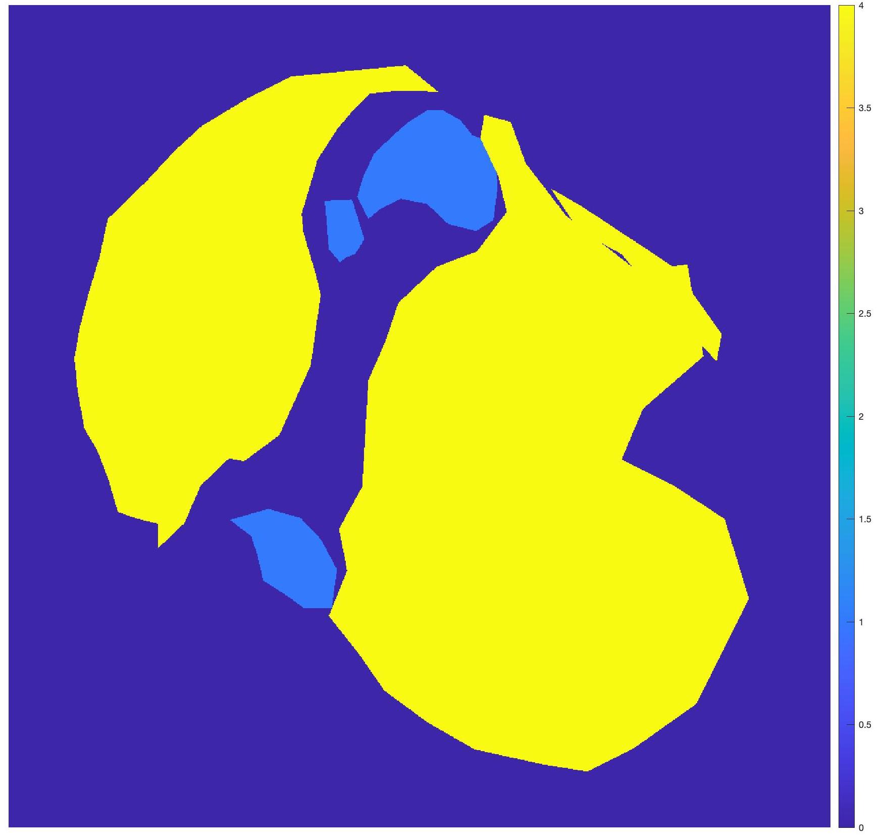
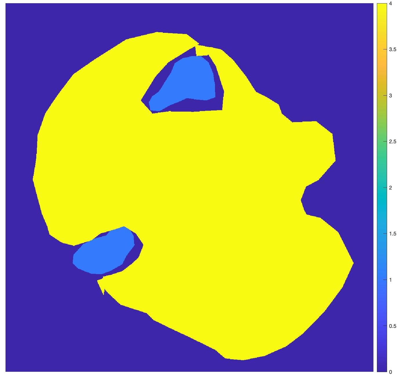
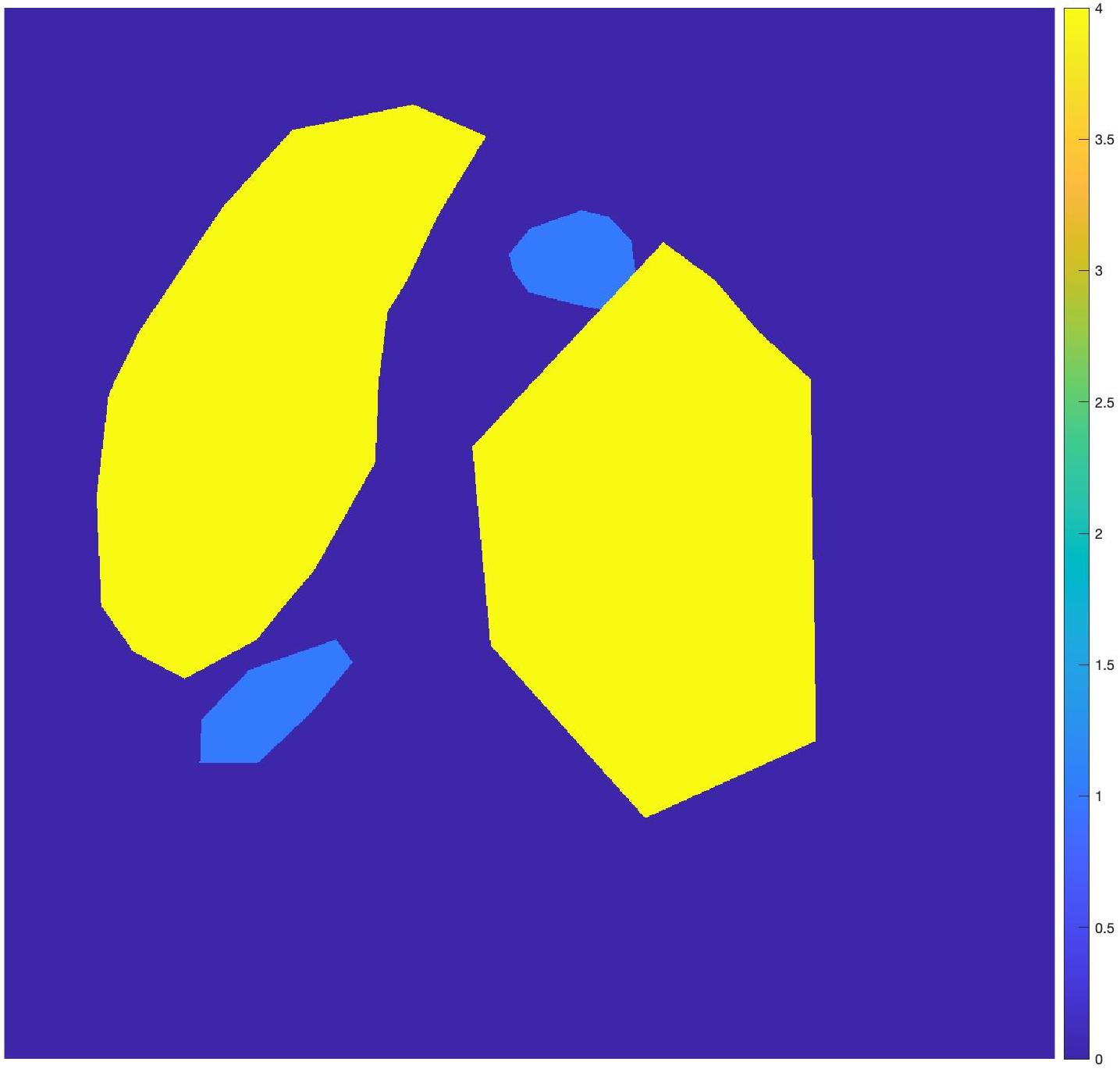
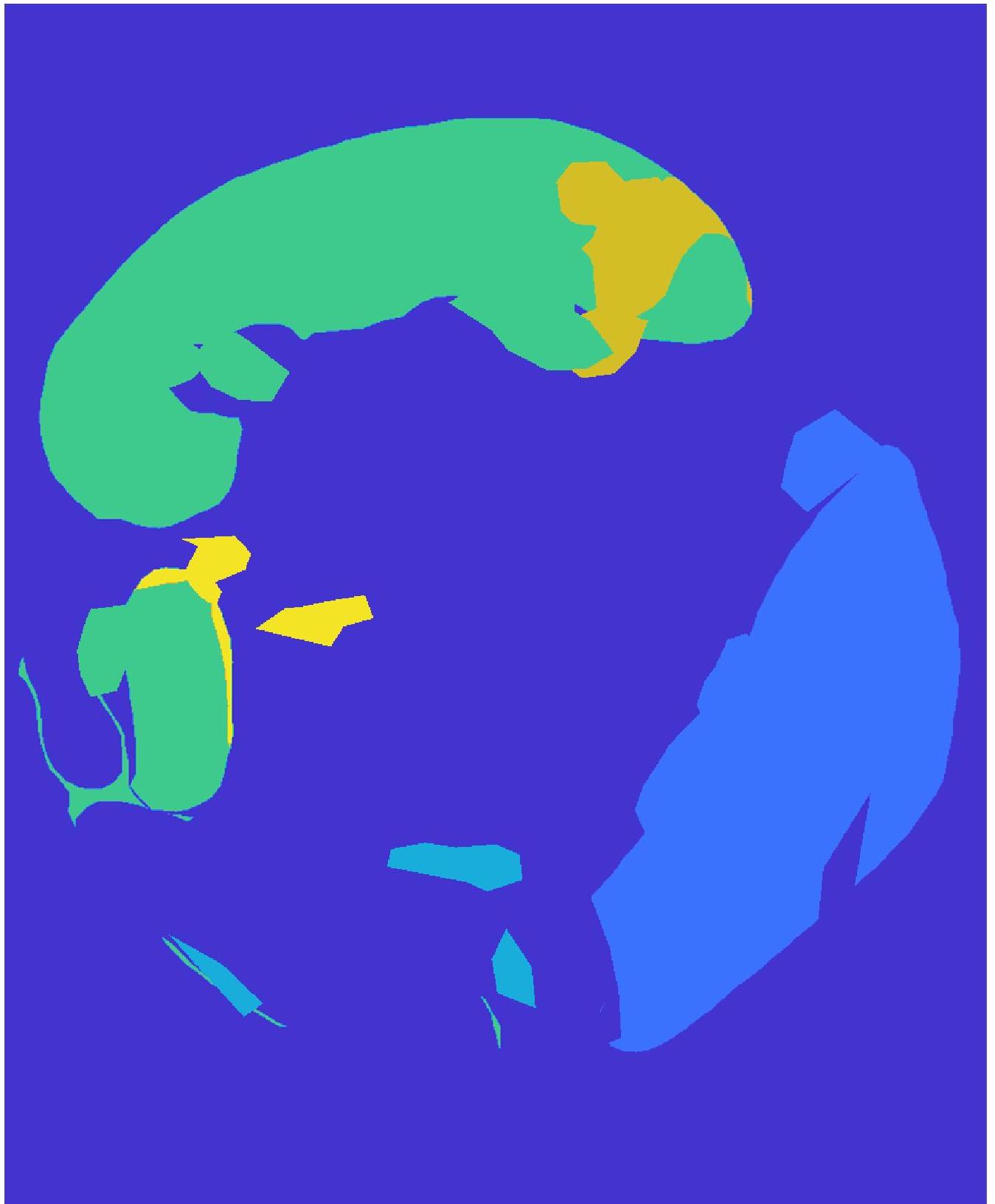
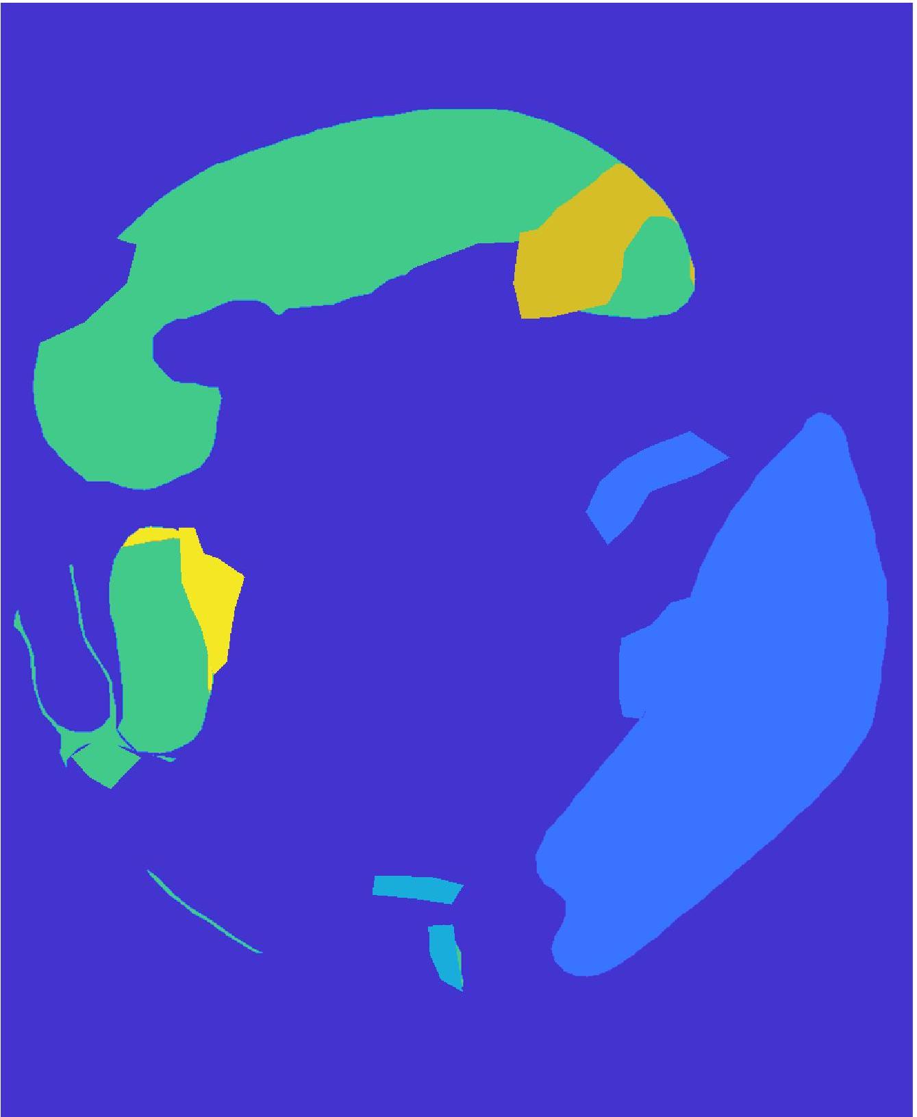
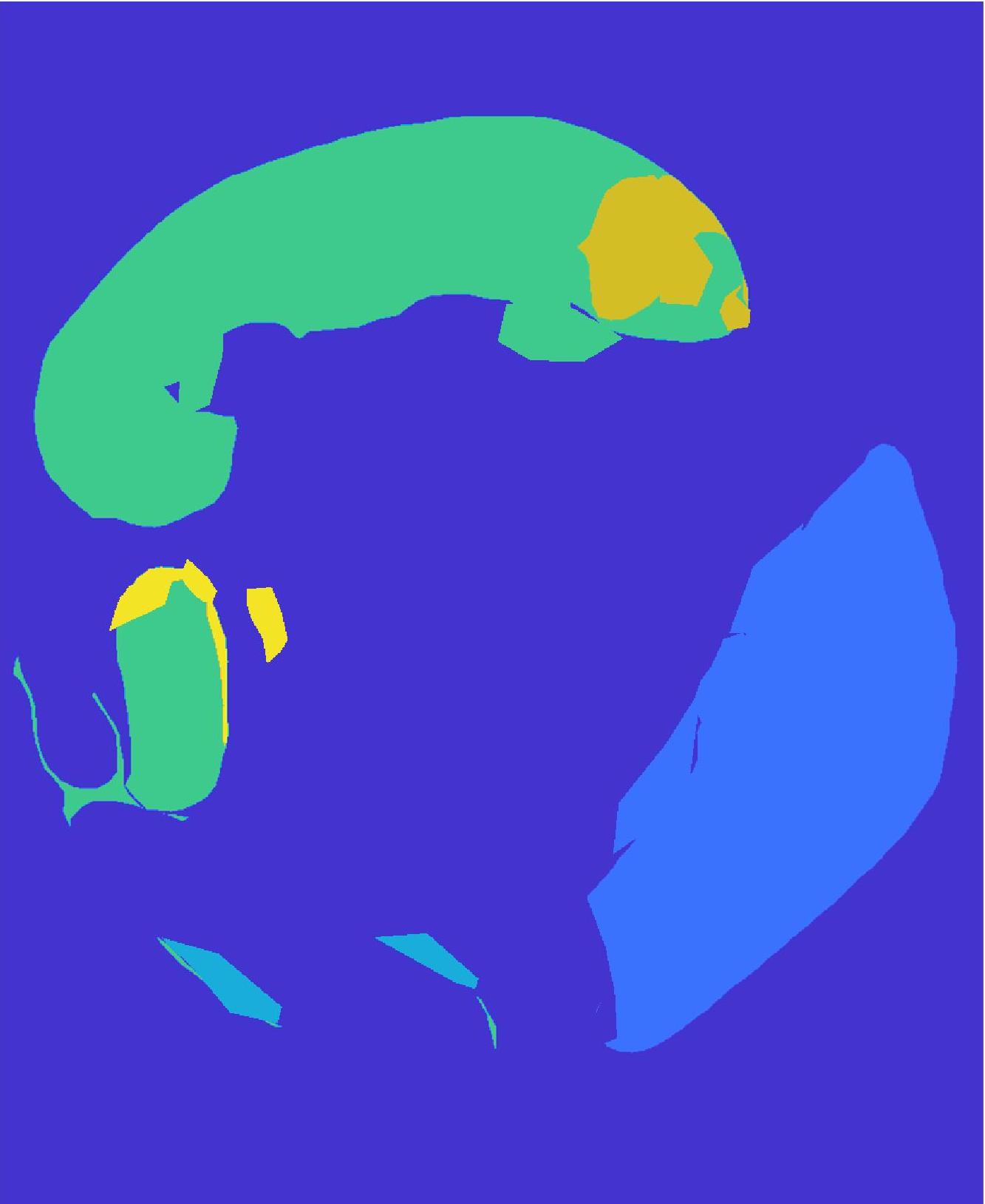
Table III summarizes the segmentation results for different ablation methods using UNet++ while Figure 7 shows the corresponding segmentation mask. The segmentation outputs are quite different from the ground truth and the one obtained by GeoGAN_WSS (Figure 6). In some cases, the normal regions are included as pathological areas, while parts of the diseased regions are not segmented. Either case is undesirable for disease diagnosis and quantification. Thus, different components of our cost functions are integral to the method’s performance. Excluding one or more of classification loss, geometric loss, and sampling loss adversely affects segmentation performance.

(a)	(b)	(c)

Figure 7: Segmentation results for ablation experiments on the training set: (a) $GeoGAN_{noL_{shape}}$; (b) $GeoGAN_{noL_{cls}}$; (c) $GeoGAN_{noSamp}$. Results correspond to the images shown in the two rows of Figure 6.

TABLE III: Mean and standard deviation (in brackets) of segmentation results from ablation studies on training dataset using the UNet++ architecture. HD is in mm.

	GeoGAN	GeoGAN	GeoGAN
	${}_{noL_{cls}}$	${}_{noL_{shape}}$	noSamp
DM	0.891(0.07)	0.899(0.08)	0.895(0.06)
HD	9.6(3.1)	9.1(3.2)	9.4(3.4)
MAE	0.071(0.015)	0.065(0.016)	0.062(0.016)

IV-E Gleason Challenge Results

The ranking of different methods is based on the overall score (Eqn 10) . The scores of GeoGAN_WSS and other methods are summarized in Table IV. Our proposed method outperforms the top-ranked method, thus clearly demonstrating the effectiveness of geometrical modeling in generating informative images. This is particularly helpful in the absence of a large dataset of annotated images.

TABLE IV: Results on the Gleason Challenge dataset for PCa detection based on overall score values.

	GeoGANWSS	Rank 1	Rank 2	Rank 3	Rank 4
Score	0.8835	0.8451	0.7925	0.7896	0.7780
	GeoGANManual	Rank 5	Rank 6	Rank 7	Rank 8
Score	0.8992	0.7597	0.7578	0.7160	0.7125

IV-F Results On Additional Datasets

IV-F1 Segmentation Results on Glas Challenge Dataset

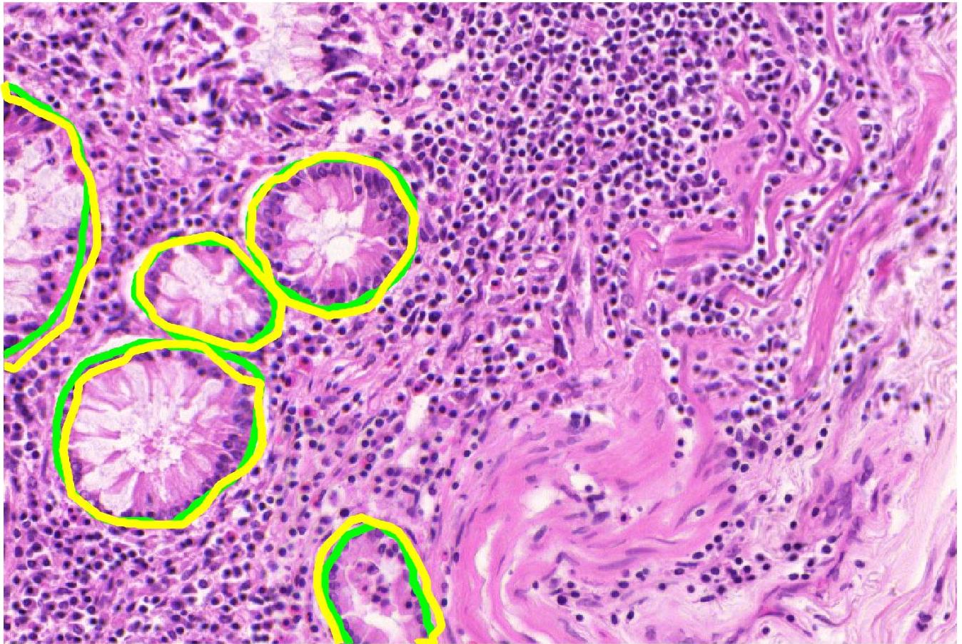
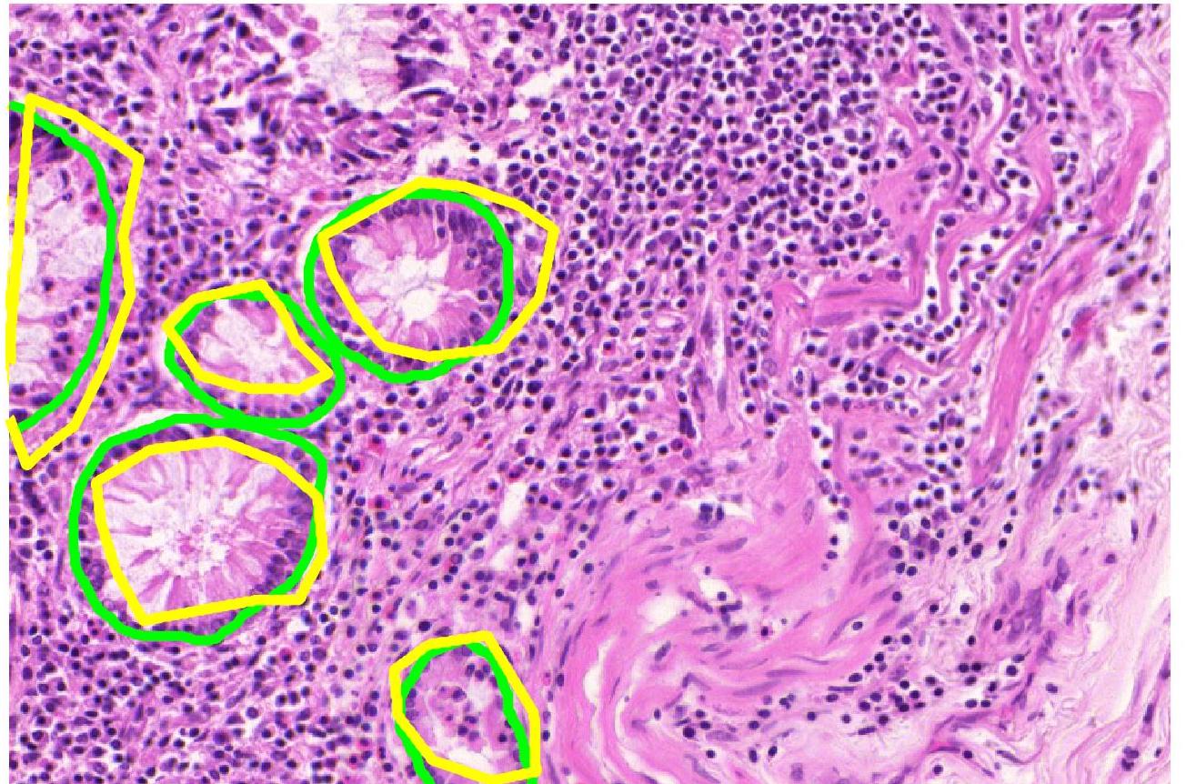
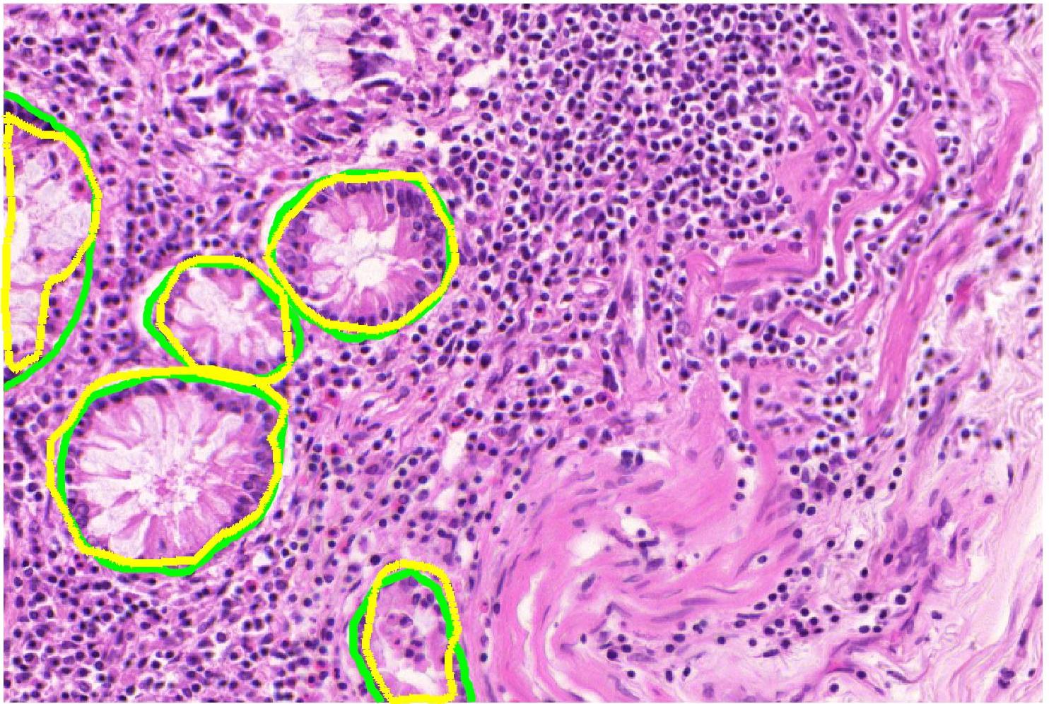
We apply our method on the public GLAS segmentation challenge [189], which has manual segmentation maps of glands in $165$ $H\&E$ stained images derived from $16$ histological sections from different patients with stage $T3$ or $T4$ colorectal adenocarcinoma. The slides were digitized with a Zeiss MIRAX MIDI Slide Scanner having pixel resolution of $0.465\mu$m. The WSIs were rescaled to a pixel resolution of $0.620\mu$m (equivalent to $20\times$ magnification). $52$ visual fields from malignant and benign areas from the WSIs were selected to cover a wide variety of tissues. An expert pathologist graded each visual field as either ‘benign’ or ‘malignant’. Further details of the dataset can be found at [189].

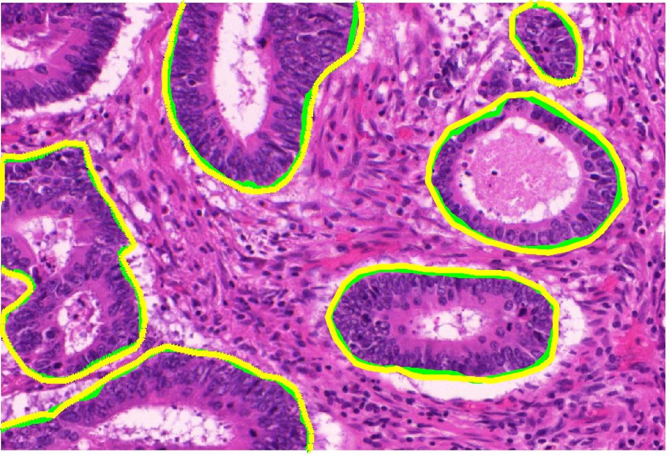
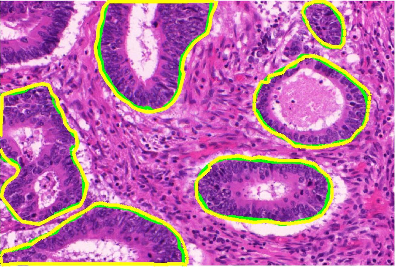
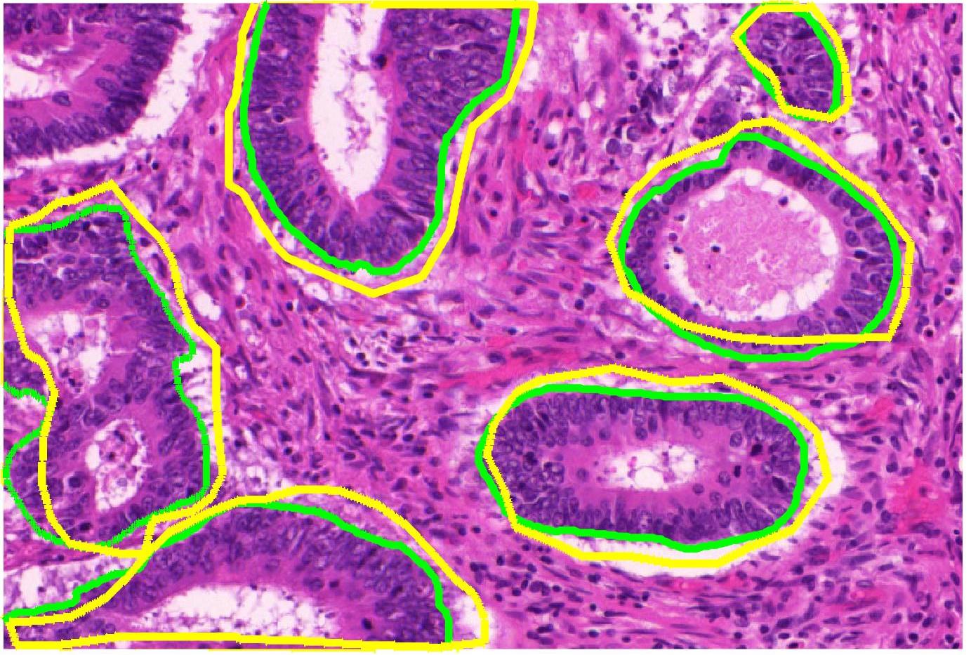
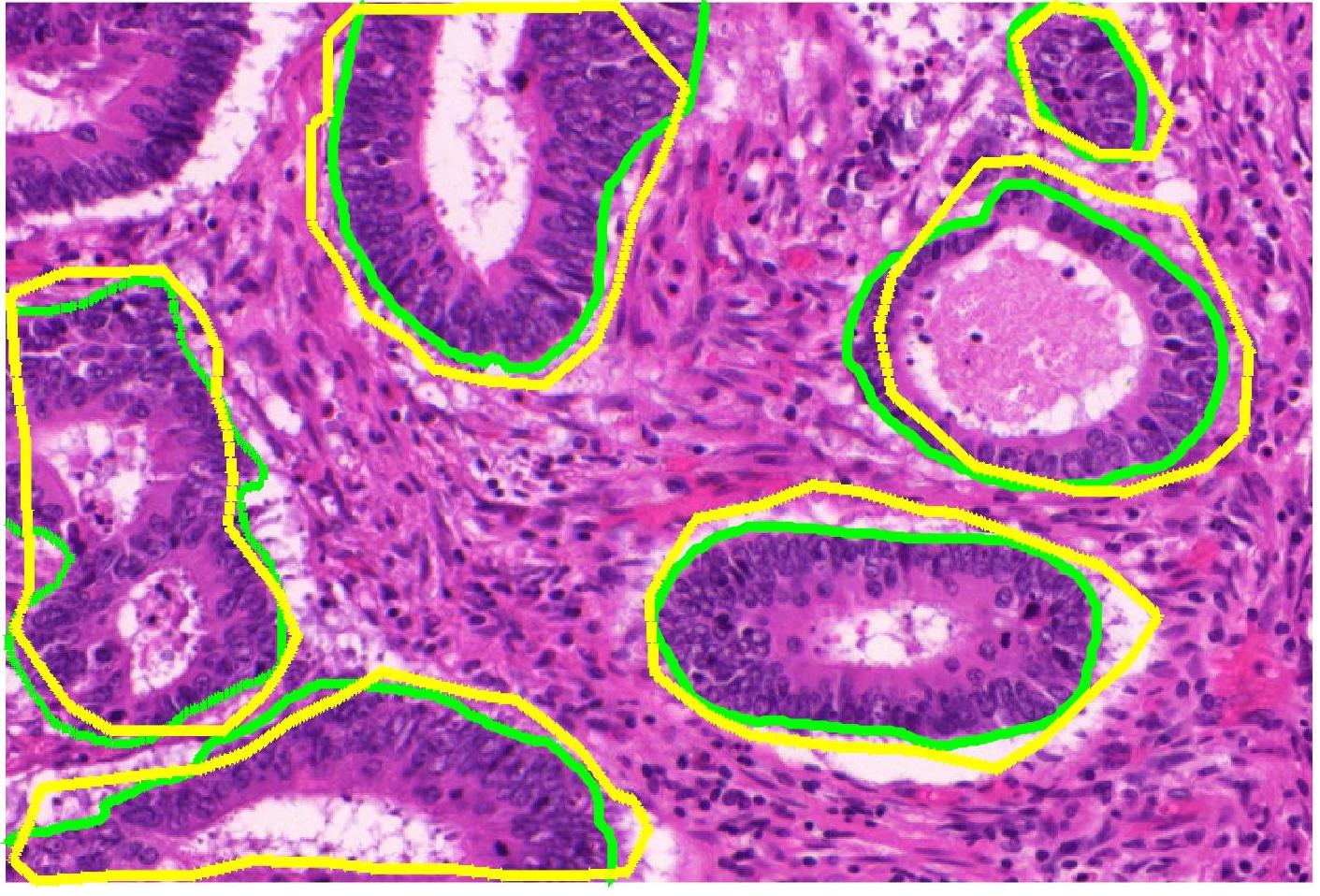
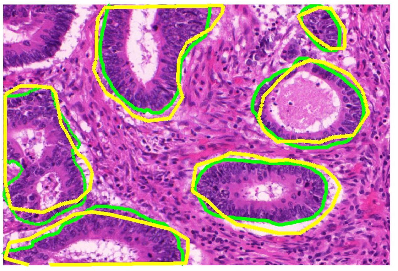
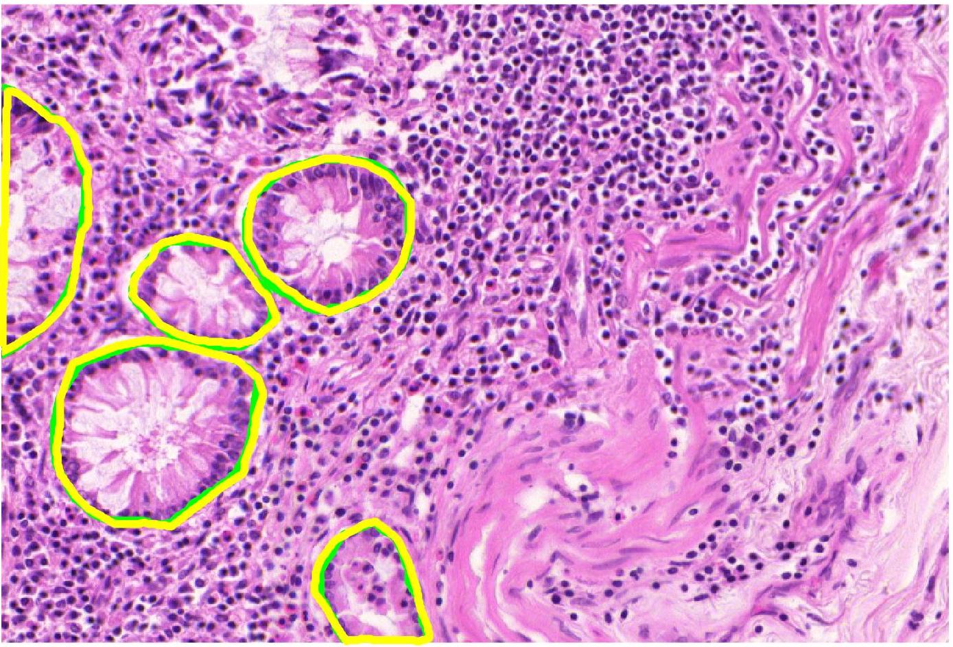
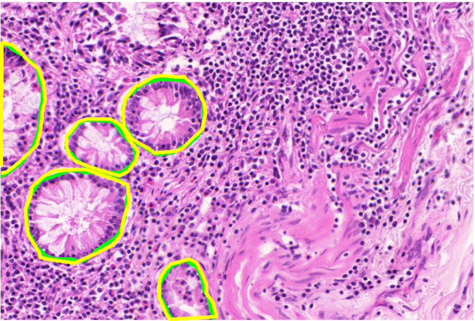
We generate augmented images using GeoGAN_WSS and train a UNet++ segmentation network to obtain the final output. The performance metrics - Dice Metric (DM), Hausdorff distance (HD), F1 score (F1)- for our results (including ablation studies) and top-ranked methods [190, 189] are summarized in Table V. The numbers are taken from the challenge paper in [189] (Table 2). Except for GeoGAN_Manual (equivalent to fully supervised training), our method, GeoGAN_WSS, outperforms all other methods using a standard segmentation architecture. The ablation study experiments’ performance also demonstrates the benefits of including all components of our proposed method. Competing methods in the challenge have used conventional augmentation, whereas our image synthesis approach generates more informative images.

Figure 8 shows example segmentation outputs of GeoGAN_WSS and other variants of our method used for ablation studies. The results clearly show that with the exclusion of our proposed method’s different components, the segmentation performance degrades.

TABLE V: Segmentation results on the GLas Segmentation challenge for GeoGAN_WSS and the top $3$ ranked methods. $HD$ is in mm. Best results per metric in bold.

	GeoGANWSS		Glas Rank 1		Glas Rank 2		GeoGANManual		GeoGAN${}_{noL_{cls}}$		GeoGAN${}_{noL_{shape}}$		GeoGANnoSamp
	Part A	Part B	Part A	Part B	Part A	Part B	Part A	Part B	Part A	Part B	Part A	Part B	Part A	Part B
F1	0.9462	0.7586	0.912	0.716	0.891	0.703	0.9514	0.7694	0.887	0.709	0.903	0.721	0.894	0.715
DM	0.9361	0.8237	0.897	0.781	0.882	0.786	0.9483	0.8361	0.878	0.757	0.892	0.784	0.883	0.761
HD	40.342	140.432	45.418	160.347	57.413	145.575	38.560	139.1842	60.234	163.459	52.32	143.321	56.34	158.753

(a)	(b)	(c)	(d)	(e)

Figure 8: Segmentation results from the GlaS Segmentation Challenge. Original image and contours of different segmentation methods are shown. The manual segmentation is shown as green contour and the algorithm output is shown in yellow for: (a) GeoGAN_Manual; (b) GeoGAN_WSS (c) GeoGAN${}_{noL_{cls}}$; (d) GeoGAN${}_{noL_{Shape}}$; (e) GeoGAN_noSamp. Rows correspond to different images.

IV-F2 Segmentation Results For CAMELYON16

We evaluate our method on the segmentation challenge part of the CAMELYON16 dataset [191] having $270$ WSIs for training and $130$ WSIs for testing. The patches are of dimension $224\times 224$ and were sampled from $10\times$ magnification WSIs (resolution of $0.972\mu m/px$) and the receptive field of a patch covers $217.8\mu$m $\times 217.8\mu$m. Segmentation output is predicted for each patch and then fused to obtain the final WSI mask. At areas of overlap we The results are summarized in Table VI. The baseline values are taken from [192] which is a recent approach using teacher-student model and reports higher values than those reported on the challenge website. Our method outperforms the baseline DenseNet121 architecture and comes close to the state of the art results of [192]. Note that the values are much higher than shown in the leaderboard since many improved methods have been proposed. This indicates that our proposed augmentation approach does very well on different datasets

TABLE VI: Results on the CAMELYON16 dataset’s segmentation challenge for GeoGAN_WSS and the state of the art results from [192].

	DenseNet121	[192]	$GeoGAN_{WSS}$	$GeoGAN_{Manual}$
DM	0.9268	0.9376	0.9311	0.9467
FROC	0.4112	0.3894	0.3982	0.3786

IV-G Comparative Analysis With Contrastive Learning Approaches

Contrastive learning approaches such as MoCo [193] and SimCLR [194] are considered state-of-the-art for downstream task based self-supervised learning u. These methods have been mostly used for classification tasks. For a fair comparison with these methods, we use our data augmentation approach for image classification on the Gleason (using the provided Gleason grades as class labels) and CAMELYON16 dataset. We follow the implementations provided by the authors, and the results are summarized in Table VII, where $ResNet$ indicates method using features derived from a ResNet [195] pre-trained with ImageNet. Both MoCo and SimCLR give similar performance, and the difference in their results is not statistically significant ($p=0.06$). Our results are close to both methods and are statistically not very different from their results. The results indicate that our pre-text task-based approach is equally effective as MoCo and SimCLR for self-supervised learning.

TABLE VII: Results on Gleason 2019 and CAMELYON16 dataset’s classification challenge. Comparison with other self supervised learning approaches using contrastive loss. $p-$values are with respect to GeoGAN_WSS.

CAMELYON16 Results
	MoCo	SimCLR	GeoGAN	GeoGAN	ResNet
	[193]	[194]	WSS	Manual
Acc	0.9012	0.8965	0.8921	0.9032	0.8323
AUC	0.9253	0.9181	0.9171	0.9231	0.8542
$p-$val	0.054	0.067	-	0.062	0.001
Gleason 2019 Results
	MoCo	SimCLR	GeoGAN	GeoGAN	ResNet
	[193]	[194]	WSS	Manual
Acc	0.9191	0.9071	0.9083	0.9165	0.8124
AUC	0.9347	0.9287	0.9292	0.9332	0.8432
$p-$val	0.062	0.057	-	0.066	0.005

IV-H Failure Cases

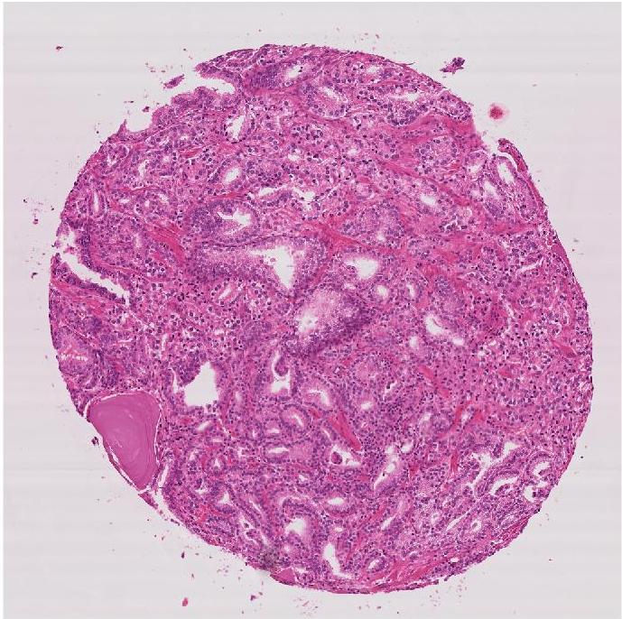
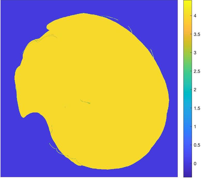
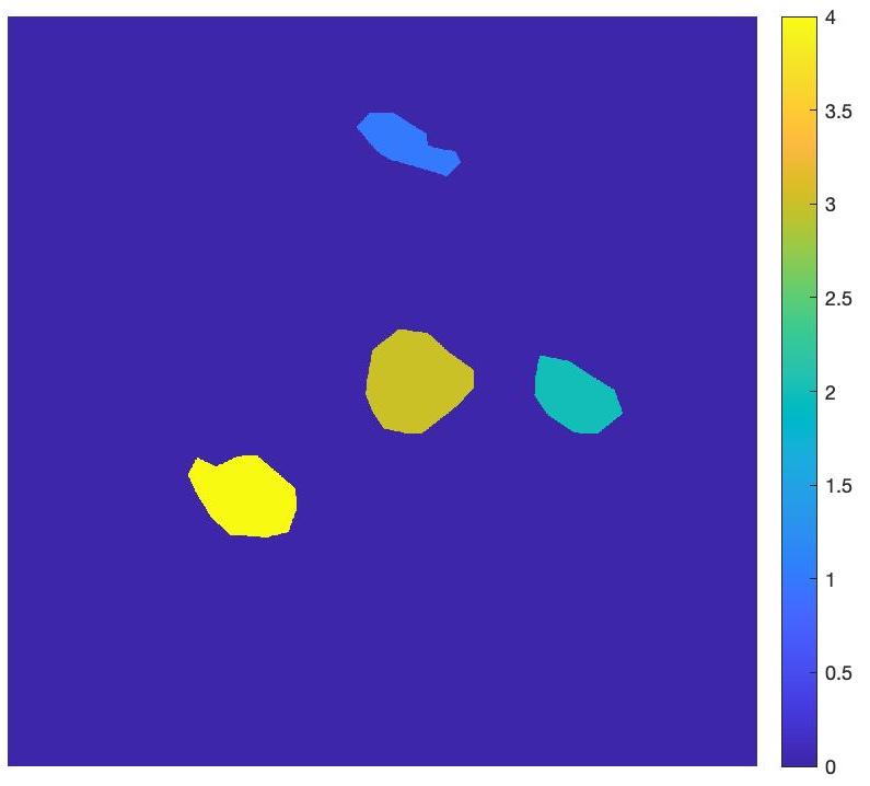
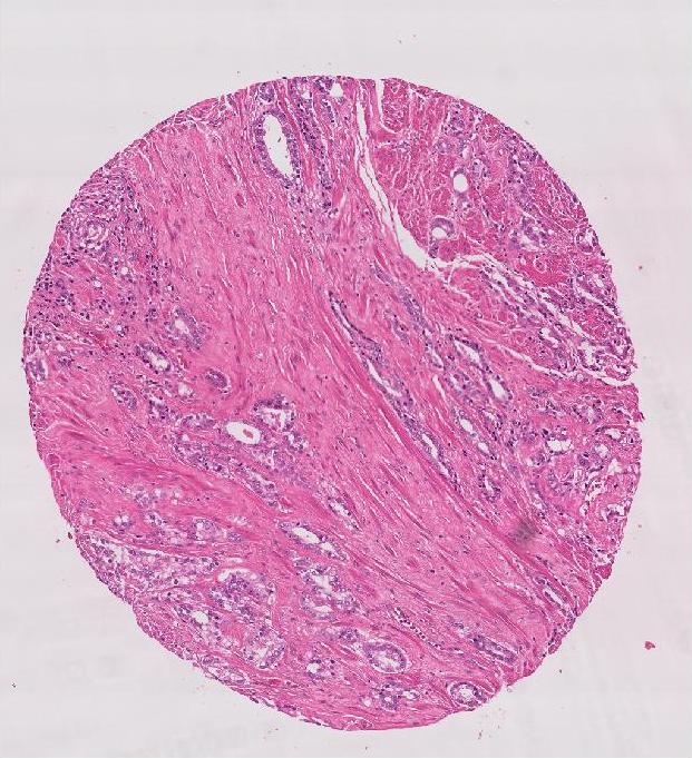
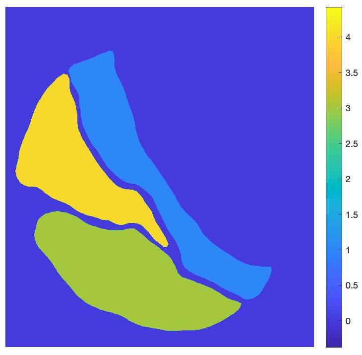
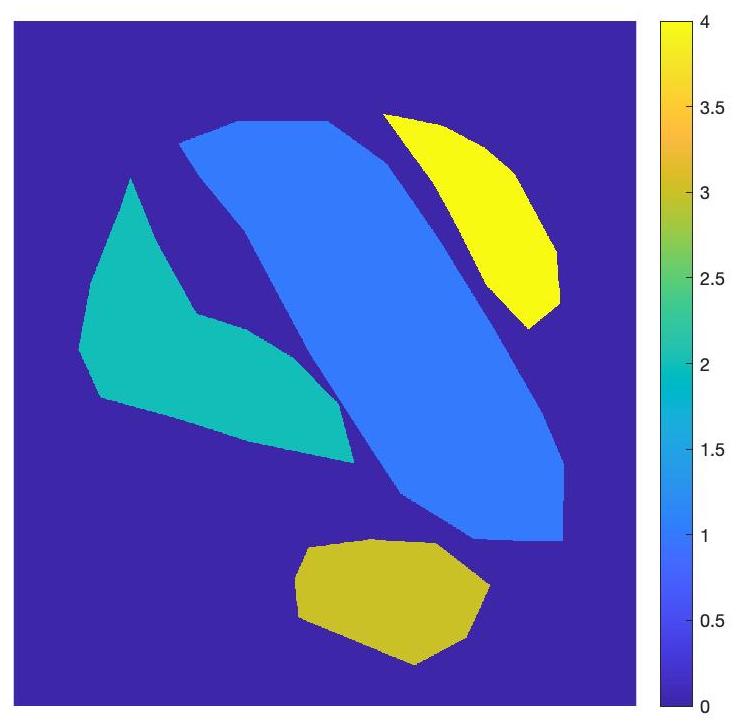
Figure 9 shows examples of some failure cases where our proposed algorithm’s segmentation had very low dice score on the Gleason dataset. The underlying reason is due to various factors such as artifacts or similar-looking structures nearby. In future work on improving the algorithm, we aim to incorporate ways to overcome the challenges posed by dissimilar tissues being too close together.

		DM$=0.37$
		DM$=0.63$
(a)	(b)	(c)

Figure 9: Examples of failure cases: (a) original image; (b) manual segmentation map; (c) segmentation map obtained using GeoGAN_WSS.

V Discussion and Conclusion

We have proposed a novel approach to generate high-quality synthetic histopathology images for segmenting Gleason graded PCa and other pathological conditions. Our method exploits the inherent geometric relationship between different segmentation labels and uses it to guide the shape generation process. We propose a self-supervised learning approach where a shape restoration network (ShaRe-Net) learns to predict the original segmentation mask from its distorted version. The pre-trained ShaRe-Net is used to extract feature maps and integrate them in the training stage. Considering the time and effort required to obtain manual segmentation maps, we propose a weakly supervised segmentation method that generates segmentation maps having high agreement with manual segmentations provided by clinicians.

We also include an uncertainty sampling stage based on a Dense UNet architecture where we inject diversity in the image generation process. The inter-label geometric relationship learnt by ShaRe-Net is leveraged by the sampling stage to generate realistic images which add diversity to the training data. Comparative results with other synthetic image generation methods show that the augmented dataset from our proposed GeoGAN_WSS method outperforms standard data augmentation and other competing methods when applied to the segmentation of PCa (from the Gleason grading challenge) and other pathologies (from CAMELYON and GlaS dataset). The synergy between shape, classification, and sampling terms leads to improved and robust segmentation and each term is important in generating realistic images. Despite the good performance of our method we observe failure cases when the base images are noisy due to inherent characteristics of the image acquisition procedure. In future work we aim to address this challenge.

Our method’s effectiveness is not limited to the Gleason dataset but also exhibits good performance on the GlaS segmentation dataset and the CAMELYON16 dataset. The high-performance gains are mainly due to learning the inter-label geometric relationships. Despite its complexity, our approach is still relevant for clinical use since it doesn’t require much effort from clinicians, shows superior performance than competing methods, and our weakly supervised segmentation step helps reduce clinician involvement.

References

- [1] J. Persson, U. Wilderäng, T. Jiborn, P. N. Wiklund, J.-E. Damber, J. Hugosson, G. Steineck, E. Haglind, and A. Bjartell, “Interobserver variability in the pathological assessment of radical prostatectomy specimens: findings of the laparoscopic prostatectomy robot open (lappro) study.” Scand. J. Urol., vol. 48, no. 2, pp. 160–167, 2014.
- [2] R. Montironia, A. Lopez-Beltran, L. Cheng, F. Montorsi, and M. Scarpelli, “Central prostate pathology review: should it be mandatory?” Eur. Urol., vol. 64, no. 2, pp. 199–201, 2013.
- [3] Y. Mikami, T. Manabe, J. Epstein, T. Shiraishi, M. Furusato, T. Tsuzuki, Y. Matsuno, and H. Sasano, “Accuracy of gleason grading by practicing pathologists and the impact of education on improving agreement,” Hum. Pathol., vol. 34, no. 7, p. 658–665, 2003.
- [4] R. Verma, N. Kumar, A. Patil, and et. al., “Monusac2020: A multi-organ nuclei segmentation and classification challenge,” IEEE TMI, pp. 1–14, 2021.
- [5] D. Mahapatra, “Registration and segmentation methodology for perfusion mr images: Application to cardiac and renal images,” -, pp. –, 2011.
- [6] S. Kuanar, D. Mahapatra, M. Bilas, and K. Rao, “Multi-path dilated convolution network for haze and glow removal in night time images,” The Visual Computer, pp. 1–14, 2021.
- [7] D. Mahapatra, A. Poellinger, L. Shao, and M. Reyes, “Interpretability-driven sample selection using self supervised learning for disease classification and segmentation,” IEEE TMI, pp. 1–15, 2021.
- [8] L. Ju, X. Wang, X. Zhao, H. Lu, D. Mahapatra, P. Bonnington, and Z. Ge, “Synergic adversarial label learning for grading retinal diseases via knowledge distillation and multi-task learning,” IEEE JBHI, vol. 100, pp. 1–14, 2020.
- [9] B. Bozorgtabar, D. Mahapatra, I. Zlobec, T. Rau, and J. Thiran, “Computational pathology.” Frontiers in Medicine, vol. 7, 2020.
- [10] D. Mahapatra and Z. Ge, “Training data independent image registration using generative adversarial networks and domain adaptation.” In press Pattern Recognition, vol. 100, pp. 1–14, 2020.
- [11] Z. Ge, D. Mahapatra, X. Chang, Z. Chen, L. Chi, and H. Lu, “Improving multi-label chest x-ray disease diagnosis by exploiting disease and health labels dependencies.” In press Multimedia Tools and Application, pp. 1–14, 2019.
- [12] B. Bozorgtabar, D. Mahapatra, and J.-P. Thiran, “Exprada: Adversarial domain adaptation for facial expression analysis.” In Press Pattern Recognition, vol. 100, pp. 15–28, 2020.
- [13] C. Han, H. Hayashi, L. Rundo, R. Araki, W. Shimoda, S. Muramatsu, Y. Furukawa, G. Mauri, and H. Nakayama, “Gan-based synthetic brain mr image generation,” in 2018 IEEE 15th International Symposium on Biomedical Imaging (ISBI 2018). IEEE, 2018, pp. 734–738.
- [14] C. Nielsen and M. Okoniewski, “Gan data augmentation through active learning inspired sample acquisition,” in Proceedings of the IEEE Conference on Computer Vision and Pattern Recognition Workshops, 2019, pp. 109–112.
- [15] B. Bozorgtabar, D. Mahapatra, H. von Teng, A. Pollinger, L. Ebner, J.-P. Thiran, and M. Reyes, “Informative sample generation using class aware generative adversarial networks for classification of chest xrays.” Computer Vision and Image Understanding, vol. 184, pp. 57–65, 2019.
- [16] ——, “Informative sample generation using class aware generative adversarial networks for classification of chest xrays.” Computer Vision and Image Understanding, vol. 184, pp. 57–65, 2019.
- [17] D. Mahapatra, B. Bozorgtabar, and R. Garnavi, “Image super-resolution using progressive generative adversarial networks for medical image analysis.” Computerized Medical Imaging and Graphics, vol. 71, pp. 30–39, 2019.
- [18] D. Mahapatra, “Semi-supervised learning and graph cuts for consensus based medical image segmentation.” Pattern Recognition, vol. 63, no. 1, pp. 700–709, 2017.
- [19] J. Zilly, J. Buhmann, and D. Mahapatra, “Glaucoma detection using entropy sampling and ensemble learning for automatic optic cup and disc segmentation.” In Press Computerized Medical Imaging and Graphics, vol. 55, no. 1, pp. 28–41, 2017.
- [20] D. Mahapatra, F. Vos, and J. Buhmann, “Active learning based segmentation of crohns disease from abdominal mri.” Computer Methods and Programs in Biomedicine, vol. 128, no. 1, pp. 75–85, 2016.
- [21] D. Mahapatra and J. Buhmann, “Visual saliency based active learning for prostate mri segmentation.” SPIE Journal of Medical Imaging, vol. 3, no. 1, 2016.
- [22] D. Mahapatra, “Combining multiple expert annotations using semi-supervised learning and graph cuts for medical image segmentation.” Computer Vision and Image Understanding, vol. 151, no. 1, pp. 114–123, 2016.
- [23] Z. Li, D. Mahapatra, J.Tielbeek, J. Stoker, L. van Vliet, and F. Vos, “Image registration based on autocorrelation of local structure.” IEEE Trans. Med. Imaging, vol. 35, no. 1, pp. 63–75, 2016.
- [24] D. Mahapatra, “An automated approach to cardiac rv segmentation from mri using learned semantic information and graph cuts.” J. Digit. Imaging., vol. 27, no. 6, pp. 794–804, 2014.
- [25] D. Mahapatra, S. Gilani, and M. Saini., “Coherency based spatio-temporal saliency detection for video object segmentation.” IEEE Journal of Selected Topics in Signal Processing., vol. 8, no. 3, pp. 454–462, 2014.
- [26] D. Mahapatra and J. Buhmann, “Analyzing training information from random forests for improved image segmentation.” IEEE Trans. Imag. Proc., vol. 23, no. 4, pp. 1504–1512, 2014.
- [27] I. Goodfellow, J. Pouget-Abadie, M. Mirza, B. Xu, D. Warde-Farley, S. Ozair, A. Courville, and Y. Bengio, “Generative adversarial nets,” in Advances in neural information processing systems, 2014, pp. 2672–2680.
- [28] D. Mahapatra and J. Buhmann, “Prostate mri segmentation using learned semantic knowledge and graph cuts.” IEEE Trans. Biomed. Engg., vol. 61, no. 3, pp. 756–764, 2014.
- [29] D. Mahapatra, J.Tielbeek, J. Makanyanga, J. Stoker, S. Taylor, F. Vos, and J. Buhmann, “Automatic detection and segmentation of crohn’s disease tissues from abdominal mri.” IEEE Trans. Med. Imaging, vol. 32, no. 12, pp. 1232–1248, 2013.
- [30] D. Mahapatra, J.Tielbeek, F. Vos, and J. Buhmann, “A supervised learning approach for crohn’s disease detection using higher order image statistics and a novel shape asymmetry measure.” J. Digit. Imaging, vol. 26, no. 5, pp. 920–931, 2013.
- [31] D. Mahapatra, “Cardiac mri segmentation using mutual context information from left and right ventricle.” J. Digit. Imaging, vol. 26, no. 5, pp. 898–908, 2013.
- [32] ——, “Cardiac image segmentation from cine cardiac mri using graph cuts and shape priors.” J. Digit. Imaging, vol. 26, no. 4, pp. 721–730, 2013.
- [33] ——, “Joint segmentation and groupwise registration of cardiac perfusion images using temporal information.” J. Digit. Imaging, vol. 26, no. 2, pp. 173–182, 2013.
- [34] D. Mahapatra and M. Saini, “A particle filter framework for object tracking using visual-saliency information.” Intelligent Multimedia Surveillance, pp. 133–147, 2013.
- [35] D. Mahapatra, “Skull stripping of neonatal brain mri: Using prior shape information with graphcuts.” J. Digit. Imaging, vol. 25, no. 6, pp. 802–814, 2012.
- [36] D. Mahapatra and Y. Sun, “Integrating segmentation information for improved mrf-based elastic image registration.” IEEE Trans. Imag. Proc., vol. 21, no. 1, pp. 170–183, 2012.
- [37] ——, “Mrf based intensity invariant elastic registration of cardiac perfusion images using saliency information,” IEEE Trans. Biomed. Engg., vol. 58, no. 4, pp. 991–1000, 2011.
- [38] Y. Xue, Q. Zhou, J. Ye, R. Long, S. Antani, C. Cornwell, Z. Xue, and X. Huang, “Synthetic augmentation and feature-based filtering for improved cervial histopathology image classification.” in MICCAI., 2019, pp. 387–396.
- [39] L. Gupta, B. Klinkhammer, P. Boor, D. Merhof, and M. Gadermayr, “Gan-based image enrichment in digital pathology boosts segmentation accuracy.” in MICCAI., 2019, pp. 631–639.
- [40] A. Antoniou, A. Storkey, and H. Edwards, “Data augmentation generative adversarial networks,” in arXiv preprint arXiv:1711.04340,, 2017.
- [41] D. Mahapatra, B. Bozorgtabar, J.-P. Thiran, and M. Reyes, “Efficient active learning for image classification and segmentation using a sample selection and conditional generative adversarial network,” in MICCAI, 2018, pp. 580–588.
- [42] D. Mahapatra, B. Bozorgtabar, and L. Shao, “Pathological retinal region segmentation from oct images using geometric relation based augmentation,” in In Proc. IEEE CVPR, 2020, pp. 9611–9620.
- [43] Y. Yamamoto, T. Tsuzuki, J. Akatsuka, and et al., “Automated acquisition of explainable knowledge from unannotated histopathology images,” Nat Commun, vol. 10, no. 5642, pp. https://doi.org/10.1038/s41 467–019–13 647–8, 2019.
- [44] X. Li, H. Chen, X. Qi, Q. Dou, C.-W. Fu, and P.-A. Heng, “H-DenseUNet: Hybrid densely connected unet for liver and tumor segmentation from ct volumes,” IEEE Trans. Med. Imag., vol. 37, no. 12, pp. 2663–2674, 2018.
- [45] S. Doyle, M. Hwang, K. Shah, and et al, “Automated grading of prostate cancer using architectural and textural image features,” in Proc. IEEE ISBI, 2007, pp. 1284–1287.
- [46] D. Mahapatra and Y. Sun, “Rigid registration of renal perfusion images using a neurobiology based visual saliency model,” EURASIP Journal on Image and Video Processing., pp. 1–16, 2010.
- [47] D. Mahapatra, “Registration and segmentation methodology for perfusion mr images: Application to cardiac and renal images,” -, pp. –, 2011.
- [48] ——, “Elastic registration of cardiac perfusion images using saliency information,” Sequence and Genome Analysis – Methods and Applications, pp. 351–364, 2011.
- [49] A. Pandey, B. Paliwal, A. Dhall, R. Subramanian, and D. Mahapatra, “This explains that: Congruent image–report generation for explainable medical image analysis with cyclic generative adversarial networks,” in In MICCAI-iMIMIC 2021, 2021, pp. 1–11.
- [50] S. Srivastava, M. Yaqub, K. Nandakumar, Z. Ge, and D. Mahapatra, “Continual domain incremental learning for chest x-ray classification in low-resource clinical settings,” in In MICCAI-FAIR 2021, 2021, pp. 1–11.
- [51] D. Mahapatra, S. Kuanar, B. Bozorgtabar, and Z. Ge, “Self-supervised learning of inter-label geometric relationships for gleason grade segmentation,” in In MICCAI-DART 2021, 2021, pp. 1–11.
- [52] D. Mahapatra, B. Bozorgtabar, S. Kuanar, and Z. Ge, “Self-supervised multimodal generalized zero shot learning for gleason grading,” in In MICCAI-DART 2021, 2021, pp. 1–11.
- [53] L. Ju, X. Wang, X. Zhao, H. Lu, D. Mahapatra, and Z. Ge, “Relational subsets knowledge distillation for long-tailed retinal diseases recognition,” in In MICCAI 2021, 2021, pp. 1–11.
- [54] J. Tong, D. Mahapatra, P. Bonnington, T. Drummond, and Z. Ge, “Registration of histopathology images using self supervised fine grained feature maps,” in In Proc. MICCAI-DART Workshop, 2020, pp. 41–51.
- [55] D. Mahapatra, B. Bozorgtabar, J.-P. Thiran, and L. Shao, “Structure preserving stain normalization of histopathology images using self supervised semantic guidance,” in In Proc. MICCAI, 2020, pp. 309–319.
- [56] B. Bozorgtabar, D. Mahapatra, J.-P. Thiran, and L. Shao, “SALAD: Self-supervised aggregation learning for anomaly detection on x-rays,” in In Proc. MICCAI, 2020, pp. 468–478.
- [57] L. Hou, D. Samaras, T. Kurc, Y. Gao, J. Davis, and J. Saltz, “Patch-based convolutional neural network for whole slide tissue image classification,” in Proc. IEEE CVPR, 2016, pp. 2424–2433.
- [58] Y. Xu, Z. Jia, L. Wang, Y. Ai, F. Zhang, M. Lai, I. Eric, and C. Chang, “Large scale tissue histopathology image classification, segmentation, and visualization via deep convolutional activation features.” BMC bioinformatics, vol. 18, no. 1, pp. 1–17, 2017.
- [59] S. Kuanar, V. Athitsos, D. Mahapatra, K. Rao, Z. Akhtar, and D. Dasgupta, “Low dose abdominal ct image reconstruction: An unsupervised learning based approach,” in In Proc. IEEE ICIP, 2019, pp. 1351–1355.
- [60] B. Bozorgtabar, M. S. Rad, D. Mahapatra, and J.-P. Thiran, “Syndemo: Synergistic deep feature alignment for joint learning of depth and ego-motion,” in In Proc. IEEE ICCV, 2019.
- [61] Y. Xing, Z. Ge, R. Zeng, D. Mahapatra, J. Seah, M. Law, and T. Drummond, “Adversarial pulmonary pathology translation for pairwise chest x-ray data augmentation,” in In Proc. MICCAI, 2019, pp. 757–765.
- [62] D. Mahapatra and Z. Ge, “Training data independent image registration with gans using transfer learning and segmentation information,” in In Proc. IEEE ISBI, 2019, pp. 709–713.
- [63] D. Mahapatra, S. Bozorgtabar, J.-P. Thiran, and M. Reyes, “Efficient active learning for image classification and segmentation using a sample selection and conditional generative adversarial network,” in In Proc. MICCAI (2), 2018, pp. 580–588.
- [64] D. Mahapatra, Z. Ge, S. Sedai, and R. Chakravorty., “Joint registration and segmentation of xray images using generative adversarial networks,” in In Proc. MICCAI-MLMI, 2018, pp. 73–80.
- [65] S. Sedai, D. Mahapatra, B. Antony, and R. Garnavi, “Joint segmentation and uncertainty visualization of retinal layers in optical coherence tomography images using bayesian deep learning,” in In Proc. MICCAI-OMIA, 2018, pp. 219–227.
- [66] S. Sedai, D. Mahapatra, Z. Ge, R. Chakravorty, and R. Garnavi, “Deep multiscale convolutional feature learning for weakly supervised localization of chest pathologies in x-ray images,” in In Proc. MICCAI-MLMI, 2018, pp. 267–275.
- [67] D. Mahapatra, B. Antony, S. Sedai, and R. Garnavi, “Deformable medical image registration using generative adversarial networks,” in In Proc. IEEE ISBI, 2018, pp. 1449–1453.
- [68] G. Litjens and et al, “Deep learning as a tool for increased accuracy and efficiency of histopathological diagnosis,” Sci Rep, vol. 6, 2016.
- [69] O. del Toro and et al, “Convolutional neural networks for an automatic classification of prostate tissue slides with high–grade Gleason score,” in Medical Imaging 2017: Digital Pathology, 2017, pp. 165–173.
- [70] S. Sedai, D. Mahapatra, S. Hewavitharanage, S. Maetschke, and R. Garnavi, “Semi-supervised segmentation of optic cup in retinal fundus images using variational autoencoder,,” in In Proc. MICCAI, 2017, pp. 75–82.
- [71] D. Mahapatra, S. Bozorgtabar, S. Hewavitahranage, and R. Garnavi, “Image super resolution using generative adversarial networks and local saliencymaps for retinal image analysis,,” in In Proc. MICCAI, 2017, pp. 382–390.
- [72] P. Roy, R. Tennakoon, K. Cao, S. Sedai, D. Mahapatra, S. Maetschke, and R. Garnavi, “A novel hybrid approach for severity assessment of diabetic retinopathy in colour fundus images,,” in In Proc. IEEE ISBI, 2017, pp. 1078–1082.
- [73] P. Roy, R. Chakravorty, S. Sedai, D. Mahapatra, and R. Garnavi, “Automatic eye type detection in retinal fundus image using fusion of transfer learning and anatomical features,” in In Proc. DICTA, 2016, pp. 1–7.
- [74] R. Tennakoon, D. Mahapatra, P. Roy, S. Sedai, and R. Garnavi, “Image quality classification for dr screening using convolutional neural networks,” in In Proc. MICCAI-OMIA, 2016, pp. 113–120.
- [75] S. Sedai, P. Roy, D. Mahapatra, and R. Garnavi, “Segmentation of optic disc and optic cup in retinal images using coupled shape regression,” in In Proc. MICCAI-OMIA, 2016, pp. 1–8.
- [76] D. Mahapatra, “Retinal image quality classification using neurobiological models of the human visual system,” in In Proc. MICCAI-OMIA, 2016, pp. 1–8.
- [77] D. Mahapatra, P. Roy, S. Sedai, and R. Garnavi, “Retinal image quality classification using saliency maps and cnns,” in In Proc. MICCAI-MLMI, 2016, pp. 172–179.
- [78] S. Sedai, P. Roy, D. Mahapatra, and R. Garnavi, “Segmentation of optic disc and optic cup in retinal fundus images using shape regression,” in In Proc. EMBC, 2016, pp. 3260–3264.
- [79] D. Mahapatra, P. Roy, S. Sedai, and R. Garnavi, “A cnn based neurobiology inspired approach for retinal image quality assessment,” in In Proc. EMBC, 2016, pp. 1304–1307.
- [80] N. Ing, Z. Ma, J. Li, H. Salemi, C. Arnold, B. S. Knudsen, and A. Gertych, “Semantic segmentation for prostate cancer grading by convolutional neural networks,” in Medical Imaging 2018: Digital Pathology, 2018, pp. 343 – 355.
- [81] J. Zilly, J. Buhmann, and D. Mahapatra, “Boosting convolutional filters with entropy sampling for optic cup and disc image segmentation from fundus images,” in In Proc. MLMI, 2015, pp. 136–143.
- [82] D. Mahapatra and J. Buhmann, “Visual saliency based active learning for prostate mri segmentation,” in In Proc. MLMI, 2015, pp. 9–16.
- [83] ——, “Obtaining consensus annotations for retinal image segmentation using random forest and graph cuts,” in In Proc. OMIA, 2015, pp. 41–48.
- [84] ——, “A field of experts model for optic cup and disc segmentation from retinal fundus images,” in In Proc. IEEE ISBI, 2015, pp. 218–221.
- [85] D. Mahapatra, Z. Li, F. Vos, and J. Buhmann, “Joint segmentation and groupwise registration of cardiac dce mri using sparse data representations,” in In Proc. IEEE ISBI, 2015, pp. 1312–1315.
- [86] D. Mahapatra, F. Vos, and J. Buhmann, “Crohn’s disease segmentation from mri using learned image priors,” in In Proc. IEEE ISBI, 2015, pp. 625–628.
- [87] H. Kuang, B. Guthier, M. Saini, D. Mahapatra, and A. E. Saddik, “A real-time smart assistant for video surveillance through handheld devices.” in In Proc: ACM Intl. Conf. Multimedia, 2014, pp. 917–920.
- [88] D. Mahapatra, J.Tielbeek, J. Makanyanga, J. Stoker, S. Taylor, F. Vos, and J. Buhmann, “Combining multiple expert annotations using semi-supervised learning and graph cuts for crohn’s disease segmentation,” in In Proc: MICCAI-ABD, 2014.
- [89] P. Schffler, D. Mahapatra, J. Tielbeek, F. Vos, J. Makanyanga, D. Pends, C. Nio, J. Stoker, S. Taylor, and J. Buhmann, “Semi automatic crohns disease severity assessment on mr imaging,” in In Proc: MICCAI-ABD, 2014.
- [90] P. J. Schueffler, D. Mahapatra, F. M. Vos, and J. M. Buhmann, “Computer aided crohn’s disease severity assessment in mri.” in VIGOR++ Workshop 2014-Showcase of Research Outcomes and Future Outlook, 2014, pp. –.
- [91] P. Leo and et al, “Stable and discriminating features are predictive of cancer presence and Gleason grade in radical prostatectomy specimens: a multi-site study,” Sci Rep, vol. 8, 2018.
- [92] D. Mahapatra, J.Tielbeek, J. Makanyanga, J. Stoker, S. Taylor, F. Vos, and J. Buhmann, “Active learning based segmentation of crohn’s disease using principles of visual saliency,” in Proc. IEEE ISBI, 2014, pp. 226–229.
- [93] D. Mahapatra, P. Schffler, J. Tielbeek, F. Vos, and J. Buhmann, “Semi-supervised and active learning for automatic segmentation of crohn’s disease,” in Proc. MICCAI, Part 2, 2013, pp. 214–221.
- [94] P. Schffler, D. Mahapatra, J. Tielbeek, F. Vos, J. Makanyanga, D. Pends, C. Nio, J. Stoker, S. Taylor, and J. Buhmann, “A model development pipeline for crohns disease severity assessment from magnetic resonance images,” in In Proc: MICCAI-ABD, 2013.
- [95] D. Mahapatra, “Graph cut based automatic prostate segmentation using learned semantic information,” in Proc. IEEE ISBI, 2013, pp. 1304–1307.
- [96] D. Mahapatra and J. Buhmann, “Automatic cardiac rv segmentation using semantic information with graph cuts,” in Proc. IEEE ISBI, 2013, pp. 1094–1097.
- [97] D. Mahapatra, J. Tielbeek, F. Vos, and J. Buhmann, “Weakly supervised semantic segmentation of crohn’s disease tissues from abdominal mri,” in Proc. IEEE ISBI, 2013, pp. 832–835.
- [98] D. Mahapatra, J. Tielbeek, F. Vos, and J. B. ., “Crohn’s disease tissue segmentation from abdominal mri using semantic information and graph cuts,” in Proc. IEEE ISBI, 2013, pp. 358–361.
- [99] D. Mahapatra, J. Tielbeek, F. Vos, and J. Buhmann, “Localizing and segmenting crohn’s disease affected regions in abdominal mri using novel context features,” in Proc. SPIE Medical Imaging, 2013.
- [100] D. Mahapatra, J. Tielbeek, J. Buhmann, and F. Vos, “A supervised learning based approach to detect crohn’s disease in abdominal mr volumes,” in Proc. MICCAI workshop Computational and Clinical Applications in Abdominal Imaging(MICCAI-ABD), 2012, pp. 97–106.
- [101] D. Mahapatra, “Cardiac lv and rv segmentation using mutual context information,” in Proc. MICCAI-MLMI, 2012, pp. 201–209.
- [102] ——, “Landmark detection in cardiac mri using learned local image statistics,” in Proc. MICCAI-Statistical Atlases and Computational Models of the Heart. Imaging and Modelling Challenges (STACOM), 2012, pp. 115–124.
- [103] G. Campanella, V. Silva, and T. Fuchs, “Terabyte-scale deep multiple instance learning for classification and localization in pathology,” in arXiv preprint arXiv:1805.06983, 2018.
- [104] F. M. Vos, J. Tielbeek, R. Naziroglu, Z. Li, P. Schffler, D. Mahapatra, A. Wiebel, C. Lavini, J. Buhmann, H. Hege, J. Stoker, and L. van Vliet, “Computational modeling for assessment of IBD: to be or not to be?” in Proc. IEEE EMBC, 2012, pp. 3974–3977.
- [105] D. Mahapatra, “Groupwise registration of dynamic cardiac perfusion images using temporal information and segmentation information,” in In Proc: SPIE Medical Imaging, 2012.
- [106] ——, “Neonatal brain mri skull stripping using graph cuts and shape priors,” in In Proc: MICCAI workshop on Image Analysis of Human Brain Development (IAHBD), 2011.
- [107] D. Mahapatra and Y. Sun, “Orientation histograms as shape priors for left ventricle segmentation using graph cuts,” in In Proc: MICCAI, 2011, pp. 420–427.
- [108] ——, “Joint registration and segmentation of dynamic cardiac perfusion images using mrfs.” in Proc. MICCAI, 2010, pp. 493–501.
- [109] D. Mahapatra and Y. Sun., “An mrf framework for joint registration and segmentation of natural and perfusion images,” in Proc. IEEE ICIP, 2010, pp. 1709–1712.
- [110] D. Mahapatra and Y. Sun, “Retrieval of perfusion images using cosegmentation and shape context information,” in Proc. APSIPA Annual Summit and Conference (ASC), 2010.
- [111] ——, “A saliency based mrf method for the joint registration and segmentation of dynamic renal mr images,” in Proc. ICDIP, 2010.
- [112] ——, “Nonrigid registration of dynamic renal MR images using a saliency based MRF model,” in Proc. MICCAI, 2008, pp. 771–779.
- [113] ——, “Registration of dynamic renal mr images using neurobiological model of saliency,” in Proc. ISBI, 2008, pp. 1119–1122.
- [114] D. Mahapatra, M. Saini, and Y. Sun, “Illumination invariant tracking in office environments using neurobiology-saliency based particle filter,” in IEEE ICME, 2008, pp. 953–956.
- [115] D. Mahapatra, S. Roy, and Y. Sun, “Retrieval of mr kidney images by incorporating shape information in histogram of low level features,” in In 13th International Conference on Biomedical Engineering, 2009, pp. 661–664.
- [116] D. Mahapatra and Y. Sun, “Using saliency features for graphcut segmentation of perfusion kidney images,” in In 13th International Conference on Biomedical Engineering, 2008.
- [117] D. Mahapatra, S. Winkler, and S. Yen, “Motion saliency outweighs other low-level features while watching videos,” in SPIE HVEI., 2008, pp. 1–10.
- [118] D. Mahapatra, A. Routray, and C. Mishra, “An active snake model for classification of extreme emotions,” in IEEE International Conference on Industrial Technology (ICIT), 2006, pp. 2195–2199.
- [119] K. Nagpal, , and et. al., “Development and validation of a deep learning algorithm for improving gleason scoring of prostate cancer,” NPJ Digit. Med, vol. 2, 2019.
- [120] A. Dosovitskiy, P. Fischer, J. T. Springenberg, M. Riedmiller, and T. Brox., “Discriminative unsupervised feature learning with exemplar convolutional neural networks,” IEEE Trans. Patt. Anal. Mach. Intell., vol. 38, no. 9, pp. 1734–1747, 2016.
- [121] D. Mahapatra and A. Singh, “Ct image synthesis using weakly supervised segmentation and geometric inter-label relations for covid image analysis,” in arXiv preprint arXiv:2106.10230, 2021.
- [122] D. Mahapatra, “Self-supervised learning of inter-label geometricrelationships for gleason grade segmentation,” in arXiv preprint arXiv:, 2021.
- [123] S. Kuanar, D. Mahapatra, V. Athitsos, and K. Rao, “Gated fusion network for sao filter and inter frame prediction in versatile video coding,” in arXiv preprint arXiv:2105.12229, 2021.
- [124] D. Mahapatra, “Interpretability-driven sample selection using self supervised learning for disease classification and segmentation,” in arXiv preprint arXiv:2104.06087, 2021.
- [125] S. Kuanar, V. Athitsos, D. Mahapatra, and A. Rajan, “Multi-scale deep learning architecture for nucleus detection in renal cell carcinoma microscopy image,” in arXiv preprint arXiv:2104.13557, 2021.
- [126] L. Ju, X. Wang, L. Wang, T. Liu, X. Zhao, T. Drummond, D. Mahapatra, and Z. Ge, “Relational subsets knowledge distillation for long-tailed retinal diseases recognition,” in arXiv preprint arXiv:2104.11057, 2021.
- [127] L. Ju, X. Wang, L. Wang, D. Mahapatra, X. Zhao, M. Harandi, T. Drummond, T. Liu, and Z. Ge, “Improving medical image classification with label noise using dual-uncertainty estimation,” in arXiv preprint arXiv:2103.00528, 2020.
- [128] B. Bozorgtabar, D. Mahapatra, G. Vray, and J.-P. Thiran, “Anomaly detection on x-rays using self-supervised aggregation learning,” in arXiv preprint arXiv:2010.09856, 2020.
- [129] D. Mahapatra, B. Bozorgtabar, J.-P. Thiran, and L. Shao, “Structure preserving stain normalization of histopathology images using self supervised semantic guidance,” in arXiv preprint arXiv:2008.02101, 2020.
- [130] D. Mahapatra, “Registration of histopathogy images using structural information from fine grained feature maps,” in arXiv preprint arXiv:2007.02078, 2020.
- [131] D. Mahapatra, B. Bozorgtabar, J.-P. Thiran, and L. Shao, “Pathological retinal region segmentation from oct images using geometric relation based augmentation,” in arXiv preprint arXiv:2003.14119, 2020.
- [132] M. Saini, B. Guthier, H. Kuang, D. Mahapatra, and A. Saddik, “szoom: A framework for automatic zoom into high resolution surveillance videos,” in arXiv preprint arXiv:1909.10164, 2019.
- [133] B. Bozorgtabar, D. Mahapatra, H. von Teng, A. Pollinger, L. Ebner, J.-P. Thiran, and M. Reyes, “Informative sample generation using class aware generative adversarial networks for classification of chest xrays,” in arXiv preprint arXiv:1904.10781, 2019.
- [134] D. Mahapatra, “Amd severity prediction and explainability using image registration and deep embedded clustering,” in arXiv preprint arXiv:1907.03075, 2019.
- [135] K. K. Leung, M. J. Clarkson, J. W. Bartlett, S. Clegg, C. R. J. Jr, M. W. Weiner, N. C. Fox, S. Ourselin, and A. D. N. Initiative, “Robust atrophy rate measurement in alzheimer’s disease using multi-site serial mri: tissue-specific intensity normalization and parameter selection,” Neuroimage, vol. 50, no. 2, pp. 516–523, 2010.
- [136] D. Mahapatra, “Generative adversarial networks and domain adaptation for training data independent image registration,” in arXiv preprint arXiv:1910.08593, 2019.
- [137] D. Mahapatra and Z. Ge, “Combining transfer learning and segmentation information with gans for training data independent image registration,” in arXiv preprint arXiv:1903.10139, 2019.
- [138] D. Mahapatra and B. Bozorgtabar, “Progressive generative adversarial networks for medical image super resolution,” in arXiv preprint arXiv:1902.02144, 2019.
- [139] S. Kuanar, K. Rao, D. Mahapatra, and M. Bilas, “Night time haze and glow removal using deep dilated convolutional network,” in arXiv preprint arXiv:1902.00855, 2019.
- [140] Z. Ge, D. Mahapatra, S. Sedai, R. Garnavi, and R. Chakravorty, “Chest x-rays classification: A multi-label and fine-grained problem,” in arXiv preprint arXiv:1807.07247, 2018.
- [141] D. Mahapatra, S. Sedai, and R. Garnavi, “Elastic registration of medical images with gans,” in arXiv preprint arXiv:1805.02369, 2018.
- [142] D. Mahapatra and B. Bozorgtabar, “Retinal vasculature segmentation using local saliency maps and generative adversarial networks for image super resolution,” in arXiv preprint arXiv:1710.04783, 2017.
- [143] D. Mahapatra, “Consensus based medical image segmentation using semi-supervised learning and graph cuts,” in arXiv preprint arXiv:1612.02166, 2017.
- [144] D. Mahapatra, K. Agarwal, R. Khosrowabadi, and D. Prasad, “Recent advances in statistical data and signal analysis: Application to real world diagnostics from medical and biological signals,” in Computational and mathematical methods in medicine, 2016.
- [145] P. Bastide, I. Kiral-Kornek, D. Mahapatra, S. Saha, A. Vishwanath, and S. V. Cavallar, “Crowdsourcing health improvements routes,” in US Patent App. 15/611,519, 2019.
- [146] D. Mahapatra, R. Garnavi, P. Roy, and R. Tennakoon, “System and method to teach and evaluate image grading performance using prior learned expert knowledge base,” in US Patent App. 15/459,457, 2018.
- [147] ——, “System and method to teach and evaluate image grading performance using prior learned expert knowledge base,” in US Patent App. 15/814,590, 2018.
- [148] D. Mahapatra, R. Garnavi, S. Sedai, and R. Tennakoon, “Generating an enriched knowledge base from annotated images,” in US Patent App. 15/429,735, 2018.
- [149] P. Bastide, I. Kiral-Kornek, D. Mahapatra, S. Saha, A. Vishwanath, and S. V. Cavallar, “Visual health maintenance and improvement,” in US Patent 9,993,385, 2018.
- [150] A. Zhao, G. Balakrishnan, F. Durand, J. V. Guttag, and A. V. Dalca, “Data augmentation using learned transforms for one-shot medical image segmentation,” in In Proc. CVPR, 2019, pp. 8543–8552.
- [151] H. Zhao, H. Li, S. Maurer-Stroh, and LiCheng, “Synthesizing retinal and neuronal images with generative adversarial nets.” Med. Imag. Anal, vol. 49, pp. 14–26, 2018.
- [152] H.-C. Shin, N. A. Tenenholtz, J. K. Rogers, C. G. Schwarz, M. L. Senjem, J. L. Gunter, K. Andriole, and M. Michalski, “Medical Image Synthesis for Data Augmentation and Anonymization using Generative Adversarial Networks,” in Proc. MICCAI-SASHIMI, 2018.
- [153] X. Yi, E. Walia, and P. Babyn, “Generative adversarial network in medical imaging: A review,” Med. Imag. Anal., vol. 58, 2019.
- [154] F. Milletari, N. Navab, and S.-A. Ahmadi, “V-net: Fully convolutional neural networks for volumetric medical im- age segmentation.” in Proc. Int. Conf. on 3D vision, 2016, pp. 565–571.
- [155] D. Mahapatra, R. Garnavi, S. Sedai, and R. Tennakoon, “Classification of severity of pathological condition using hybrid image representation,” in US Patent App. 15/426,634, 2018.
- [156] P. Bastide, I. Kiral-Kornek, D. Mahapatra, S. Saha, A. Vishwanath, and S. V. Cavallar, “Machine learned optimizing of health activity for participants during meeting times,” in US Patent App. 15/426,634, 2018.
- [157] D. Mahapatra, R. Garnavi, S. Sedai, R. Tennakoon, and R. Chakravorty, “Early prediction of age related macular degeneration by image reconstruction,” in US Patent App. 15/854,984, 2018.
- [158] ——, “Early prediction of age related macular degeneration by image reconstruction,” in US Patent 9,943,225, 2018.
- [159] D. Mahapatra, R. Garnavi, S. Sedai, and P. Roy, “Retinal image quality assessment, error identification and automatic quality correction,” in US Patent 9,779,492, 2017.
- [160] ——, “Joint segmentation and characteristics estimation in medical images,” in US Patent App. 15/234,426, 2017.
- [161] D. Mahapatra, S. Saha, A. Vishwanath, and P. Bastide, “Generating hyperspectral image database by machine learning and mapping of color images to hyperspectral domain,” in US Patent App. 15/949,528, 2019.
- [162] D. Mahapatra, Z. Ge, and S. Sedai, “Joint registration and segmentation of images using deep learning,” in US Patent App. 16/001,566, 2019.
- [163] R. Garnavi, D. Mahapatra, P. Roy, and R. Tennakoon, “System and method to teach and evaluate image grading performance using prior learned expert knowledge base,” in US Patent App. 10,657,838, 2020.
- [164] B. Antony, S. Sedai, D. Mahapatra, and R. Garnavi, “Real-time passive monitoring and assessment of pediatric eye health,” in US Patent App. 16/178,757, 2020.
- [165] D. Mahapatra, S. Sedai, and K. Halupka, “Uncertainty region based image enhancement,” in US Patent App. 10,832,074, 2020.
- [166] J. D. Hoog, D. Mahapatra, R. Garnavi, and F. Jalali, “Personalized monitoring of injury rehabilitation through mobile device imaging,” in US Patent App. 16/589,046, 2021.
- [167] P. Roy, D. Mahapatra, R. Garnavi, and R. Tennakoon, “System and method to teach and evaluate image grading performance using prior learned expert knowledge base,” in US Patent App. 10,984,674, 2021.
- [168] A. Kendall, V. Badrinarayanan, and R. Cipolla, “Bayesian segnet: Model uncertainty in deep convolutional encoder-decoder architectures for scene understanding.” in arXiv:1511.02680, 2015.
- [169] B. Lakshminarayanan, A. Pritzel, and C. Blundell, “Simple and scalable predictive uncertainty estimation using deep ensembles.” in Proc. NIPS, 2017, pp. 6402–6413.
- [170] C. Rupprecht, I. Laina, R. DiPietro, M. Baust, F. Tombari, N. Navab, and G. D. Hager, “Learning in an uncertain world: Representing ambiguity through multiple hypotheses.” in Proc. CVPR, 2017, pp. 3591–3600.
- [171] K. Sohn, H. Lee, and X. Yan, “Learning structured output representation using deep conditional generative models.” in Proc. NIPS, 2015, pp. 3483–3491.
- [172] S. A. A. Kohl, B. Romera-Paredes, C. Meyer, J. D. Fauw, J. R. Ledsam, K. H. Maier-Hein, S. M. A. Eslami, D. J. Rezende, and O. Ronneberger, “A probabilistic u-net for segmentation of ambiguous images.” in Proc. NIPS, 2018, pp. 6965–6975.
- [173] O. Ronneberger, P. Fischer, and T. Brox, “U-net: Convolutional networks for biomedical image segmentation,” in In Proc. MICCAI, 2015, pp. 234–241.
- [174] C. F. Baumgartner, K. C. Tezcan, K. Chaitanya, A. M. Hötker, U. J. Muehlematter, K. Schawkat, A. S. Becker, O. Donati, and E. Konukoglu, “Phiseg: Capturing uncertainty in medical image segmentation.” in Proc. MICCAI(2), 2019, pp. 119–127.
- [175] A. Jamaludin, T. Kadir, and A. Zissrman, “Self-supervised learning for spinal mris,” in Proc. Deep Learning in Medical Image Analysis and Multimodal Learning for Clinical Decision Support, 2017, pp. 294–302.
- [176] T. Ross, , and et al., “Exploiting the potential of unlabeled endoscopic video data with self-supervised learning,” International Journal of Computer Assisted Radiology and Surgery volume, vol. 13, pp. 925–933, 2018.
- [177] N. Tajbakhsh, Y. Hu, J. Cao, X. Yan, Y. Xiao, Y. Lu, J. Liang, D. Terzopoulos, and X. Ding, “Surrogate supervision for medical image analysis: Effective deep learning from limited quantities of labeled data,” in In Proc. IEEE ISBI, 2019, pp. 1251–1255.
- [178] W. Bai, C. Chen, G. Tarroni, J. Duan, F. Guitton, S. E. Petersen, Y. Guo, P. M. Matthews, and D. Rueckert, “Self-supervised learning for cardiac mr image segmentation by anatomical position prediction,” in In Proc. MICCAI, 2019, pp. 234–241.
- [179] L. Chen, P. Bentley, K. Mori, K. Misawa, M. Fujiwara, and D. Rueckert, “Self-supervised learning for medical image analysis using image context restoration,” Medical Imag. Anal., vol. 58, pp. 1–12, 2019.
- [180] N. A. Koohbanani, B. Unnikrishnan, S. A. Khurram, P. Krishnaswamy, and N. Rajpoot, “Self-path: Self-supervision for classification of pathology images with limited annotations,” in arXiv:2008.05571, 2020.
- [181] M. Y. Lu, R. J. Chen, J. Wang, D. Dillon, and F. Mahmood, “Semi-supervised histology classification using deep multiple instance learning and contrastive predictive coding,” in arXiv:1910.10825, 2019.
- [182] H. Muhammad, C. S. Sigel, G. Campanella, T. Boerner, L. M. Pak, S. Buttner, J. N. IJzermans, B. G. Koerkamp, M. Doukas, W. R. Jarnagin, A. Simpson, and T. J. Fuchs, “Towards unsupervised cancer subtyping: Predicting prognosis using a histologic visual dictionary,” in arXiv:1903.05257, 2019.
- [183] C. Leistner, A. Saffari, J. Santner, and H. Bischof, “Semi-supervised random forests,” in 2009 IEEE 12th International Conference on Computer Vision (ICCV), 2009, pp. 506–513.
- [184] Z. Zhou, M. M. R. Siddiquee, N. Tajbakhsh, and J. Liang, “Unet++: Redesigning skip connections to exploit multiscale features in image segmentation,” IEEE Trans. Med. Imag., pp. 1–10, 2019.
- [185] M. Jaderberg, K. Simonyan, A. Zisserman, and K. Kavukcuoglu, “Spatial transformer networks,” in NIPS, 2015, pp. –.
- [186] D. Karimi, G. Nir, L. Fazli, P. Black, L. Goldenberg, and S. Salcudean, “Deep learning-based gleason grading of prostate cancer from histopathology images-role of multiscale decision aggregation and data augmentation.” IEEE J Biomed Health Inform., vol. 24, no. 5, pp. 1413–1426, 2020.
- [187] D. P. Kingma and J. Ba, “Adam: A method for stochastic optimization,” in arXiv preprint arXiv:1412.6980,, 2014.
- [188] H. Zhao, J. Shi, X. Qi, X. Wang, and J. Jia, “Pyramid scene parsing network,” in CVPR, 2017.
- [189] K. Sirinukunwattana, , and et al., “Gland segmentation in colon histology images: The GlaS challenge contest,” Med. Imag. Anal., vol. 35, pp. 489–502, 2017.
- [190] “Glas segmentation challenge results,” https://warwick.ac.uk/fac/sci/dcs/research /tia/glascontest/results/, accessed: 2020-01-30.
- [191] B. E. Bejnordi, M. Veta, P. J. van Diest, B. van Ginneken, N. Karssemeijer, G. Litjens, J. van der Laak, , and the CAMELYON16 Consortium, “Diagnostic Assessment of Deep Learning Algorithms for Detection of Lymph Node Metastases in Women With Breast Cancer,” JAMA, vol. 318, no. 22, pp. 2199–2210, 2017.
- [192] H.-T. Cheng, C.-F. Yeh, P.-C. Kuo, A. Wei, K.-C. Liu, M.-C. Ko, K.-H. Chao, Y.-C. Peng, and T.-L. Liu, “Self-similarity student for partial label histopathology image segmentation,” in Proc. ECCV, 2020, pp. 1–16.
- [193] K. He, H. Fan, Y. Wu, S. Xie, and R. Girshick, “Momentum contrast for unsupervised visual representation learning,” in Proc. CVPR, 2020, pp. 9729–9738.
- [194] T. Chen, S. Kornblith, M. Norouzi, and G. Hinton, “A simple framework for contrastive learning of visual representations,” in arXiv preprint arXiv:2002.05709, 2020.
- [195] K. He, X. Zhang, S. Ren, and J. Sun, “Deep residual learning for image recognition,” in In Proc. CVPR, 2016.