Particle hopping on a ladder: exact solution using multibalance

Abstract

We study particle hopping on a two-leg ladder where a particle can jump to their immediate neighbours, one at a time, with rates that depend on the occupation of the departure site and a neighbouring site on the other leg. For specific choices of rates, the model can be solved using pairwise balance known earlier. For the other regimes, we introduce a new balance condition called multibalance which helps us in obtaining the exact steady state. The direction of the total current in these models does not necessarily decide the direction of the currents in individual legs; we find the regions in the parameter space where the currents in individual legs alter their direction. In some parameter regime, the total current exhibits the re-entrance phenomena, in the sense that the total current flips its direction with increase of certain parameter and flips it again when the parameter is increased further. It turns out that the multibalance condition we introduce here is very useful and it can be applied generically to several other models. We discuss some of these models in short.

Keywords: Zero-range processes, Non-equilibrium processes, Exact results

1 Introduction

Nonequilibrium steady states (NESS) [1, 2] differ from their equilibrium counterparts which obey detailed balance [3, 4]. Detailed balance ensures that there is no net flow of probability current among any pair of configurations leading to the well known Gibbs-Boltzmann measure in its steady state. Such a generic measure is absent in nonequilibrium and in general, finding an exact NESS measure for any nonequilibrium dynamics is usually difficult. It has been realized that exact solutions of steady state measures for certain non-equilibrium systems and analytical calculation of observables bring much insight to the understanding of the corresponding systems. In context of the exactly solvable interacting non-equilibrium systems, there exist a few successful models. The zero range process (ZRP) [5, 6, 7] and certain lattice gas models in one dimension are perhaps the simplest of them, which exhibit nontrivial static and dynamic properties in the steady state. These models have found applications in describing phase separation criteria in driven lattice gases [8], network re-wiring [9, 10], statics and dynamics of extended objects [11, 12]. etc.

The steady state of the well studied ZRP can be obtained using a pairwise balance (PWB) condition [13] where for every transition $C\to C^{\prime}$ one needs to find a unique configuration $C^{\prime\prime}$ such that the out-flux from $C$ to $C^{\prime}$ is balanced by the in-flux from $C^{\prime\prime}$ to $C$. The steady state of asymmetric simple exclusion process (ASEP) also follows the PWB condition. These models with open boundaries could be solved exactly [14] using a matrix product ansatz (MPA), where the steady state weight of any configuration is represented by a product of non-commuting matrices. This matrix product ansatz has been successfully implemented in several other models. Some examples include ASEP with open boundaries [14, 15], multiple species of particles [16] and models where particles have some internal degrees of freedom [17], non-conserved systems with deposition, evaporation, coagulation-decoagulation like dynamics [18]. Another class of nonequilibrium models, finite range processes (FRP) have been studied recently [19]. It is shown that, for certain specific conditions on hop rates, the FRP has a cluster-factorized steady state (CFSS). The steady states of these models can be achieved by both pairwise balance and $h$-balance conditions [19, 20] and they exhibit a finite dimensional transfer-matrix representation of the steady state.

In this article we introduce another balance condition, namely multibalance (MB), to non-equilibrium steady states (NESS): for every configuration $C,$ the sum of outgoing fluxes to one or more configurations are balanced here by the sum of multiple incoming fluxes. A recent article [21] has independently discussed this balance condition to exactly determine the steady state of a model namely light-heavy (LH) model. This balance condition is referred to as bunchwise balance. We applied the multibalance condition to the model of particle hopping on a two-leg ladder, where the hop rates depend on the occupation number of the departure site and corresponding occupation number in the other leg. The steady state currents in this model exhibit several interesting features. When some of the parameters of the model increased, the total current flipped its direction and further increase of the same parameter resulted in another flip of direction. Along with this re-entrance phenomena, we also find that the direction of the total current does not necessarily dictate the direction of the currents in individual legs; we explicitly obtain the line of separation where currents in individual legs alter their direction.

The new balance condition turns out to be a very useful method to obtain exact steady state of some nonequilibrium models. It can be implemented to obtain factorized or pair-factorized steady states (PFSS), which is described in section 3 and 4. We generalize the hopping rates of the two-leg ladder to obtain a PFSS when the rates satisfy the multibalance conditions. More generic models, like finite range processes which give rise to cluster-factorized steady states (CFSS) and systems with more than one species of particles are discussed briefly in section 5; exact steady states obtained for these models clearly emphasize the utility and strength of this new balance condition.

2 Multibalance (MB)

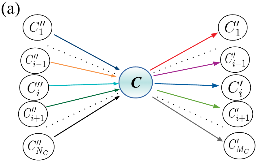
We define a generalized balance condition in nonequilibrium systems such that a bunch of fluxes coming to the configuration $C$ from a set of configurations $\{C^{\prime\prime}_{1},\cdots,C^{\prime\prime}_{N_{C}}\}$ are balanced by the sum of out-fluxes from $C$ to a set of configurations $\{C^{\prime}_{1},\cdots,C^{\prime}_{M_{C}}\}$ in the configuration space.

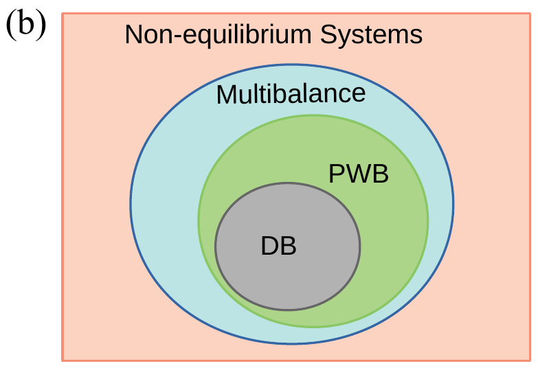
Figure 1: (a) Multibalance: fluxes are represented by arrows. Incoming fluxes to the configuration $C$ from a set of configurations $\{C^{\prime\prime}_{1},\cdots,C^{\prime\prime}_{N_{C}}\}$ are balanced with the outward fluxes from $C$ to the set of configurations $\{C^{\prime}_{1},...,C^{\prime}_{M_{C}}\}$, (b) In nonequilibrium systems, multibalance is a generalised balance condition to obtain the steady state. When $N_{C}=M_{C}=1$, PWB is a subset of multibalance for $C^{\prime\prime}_{1}\neq C_{1}^{\prime}$ and DB is a subset of PWB for $C^{\prime\prime}_{1}=C_{1}^{\prime}$, corresponds to the equilibrium case.

Here $N_{C}$ is the total number of incoming fluxes for the set of configurations $\{C^{\prime\prime}_{1},\cdots,C^{\prime\prime}_{N_{C}}\}$ and $M_{C}$ is the total number of outgoing fluxes for the set of configurations $\{C^{\prime}_{1},...,C^{\prime}_{M_{C}}\}$ as described in Fig. 1(a). At steady state, for any system, the fluxes must balance: $\sum_{C^{\prime}}P(C)W(C\rightarrow C^{\prime})=\sum_{C^{\prime\prime}}P(C^{\prime\prime})W(C^{\prime\prime}\rightarrow C)$. We have denoted $P(C)$ be the probability of the configuration $C$ and it can move to the other configuration $C^{\prime}$ with a dynamical rate $W(C\rightarrow C^{\prime})$. For systems that satisfy a multibalance, these steady state configurations break into many conditions of the form,

$$\sum_{i=1}^{M_{C}}P(C)W(C\rightarrow C^{\prime}_{i})=\sum_{i=1}^{N_{C}}P(C^{\prime\prime}_{i})W(C^{\prime\prime}_{i}\rightarrow C).$$ (1)

Eq. (1) describes that for every configuration $C$, the incoming fluxes from a group of configurations $\{C^{\prime\prime}_{1},\cdots,C^{\prime\prime}_{N_{C}}\}$, are balanced by outgoing fluxes to another uniquely identified group of configurations $\{C^{\prime}_{1},...,C^{\prime}_{M_{C}}\}$. As a special case of multibalance condition, for $N_{C}=M_{C}=1$, if $C^{\prime\prime}_{1}\neq C_{1}^{\prime}$, Eq. (1) reduces to Pairwise balance balance condition (PWB) and for the simplest case when $C^{\prime\prime}_{1}=C_{1}^{\prime}$, it becomes the well known Detailed balance condition (DB) corresponds to the equilibrium case as shown in Fig. 1(b).

2.1 Zero range process (ZRP) in two dimensions with asymmetric rates

The zero range process (ZRP) is a model in which many indistinguishable particles occupy sites on a lattice and these particles hop between neighbouring sites with a rate that depends on the number of particles at the site of departure. The steady state of ZRP can be solved exactly in any dimension for periodic boundaries and in some cases, for open boundaries [7, 22, 23].

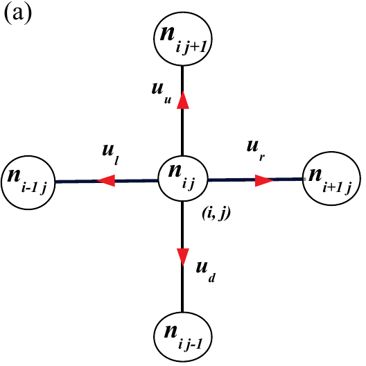
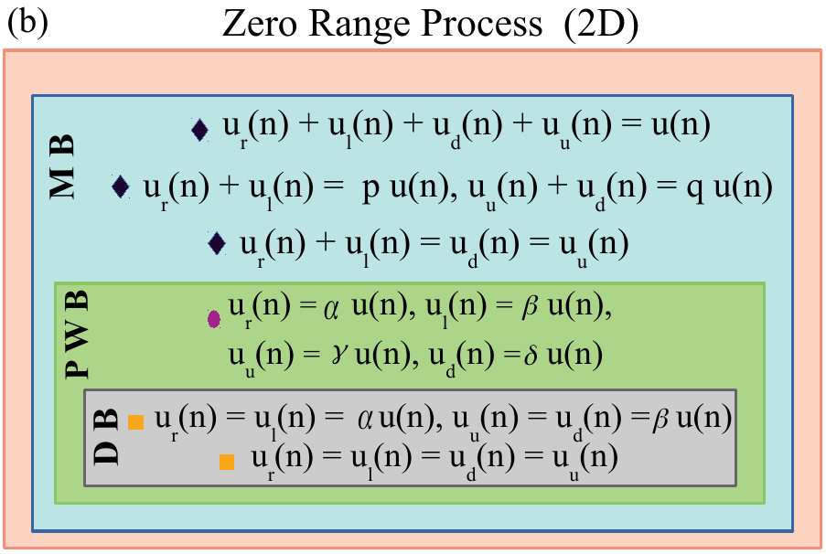
Figure 2: (a) ZRP in two dimensions, where a particle from site $(i,j)$ can hop to its right, left, up and down nearest neighbours with rates $u_{r}(n_{i,j})$, $u_{l}(n_{i,j})$, $u_{u}(n_{i,j})$ and $u_{d}(n_{i,j})$ respectively. $n_{i,j}$ is the number of particles at site $(i,j)$, (b) FSS can be obtained for this 2D ZRP model using different balance schemes - MB, PWB and DB. Examples of corresponding conditions on the hop rates are mentioned there in respective regions and the FSS can be obtained following any of these conditions. Clearly, MB is the generalized choice to obtain the FSS where the hop rates are different in all four directions.

We consider a periodic lattice in two dimensions of size ($L\times L$). Each site $(i,j)$ with, $i=1,2,\cdots L$, $j=1,2,\cdots L$, can be either vacant or it can be occupied by one or more particles $n_{i,j}\leq N$ $\left(N=\sum_{i=1}^{L}\sum_{j=1}^{L}n_{i,j}\right)$. A particle from any of the sites $(i,j)$ can hop to its nearest neighbours (right, left, up and down) with rates $u_{r}(n_{i,j})$, $u_{l}(n_{i,j})$, $u_{u}(n_{i,j})$ and $u_{d}(n_{i,j})$ respectively as shown in Fig. 2(a). We assume that the model evolves to a factorized steady state (FSS)

$$P(\{n_{i,j}\})\propto\prod_{i=1,j=1}^{L}f(n_{i,j})~{}\delta\left(\sum_{i=1,j=1}^{L}n_{i,j}-N\right).$$ (2)

$N$ is the total number of particles and the density of the system $\rho=\frac{N}{L^{2}}$ is conserved by the dynamics. Our task is to verify on what condition we can get FSS as in Eq. (2) for this model
(a) When the rates $u_{r}(n)=u_{l}(n)=\alpha u(n)$ and $u_{u}(n)=u_{d}(n)=\beta u(n)$, where both $\alpha$ and $\beta$ are constants or $u_{r}(n)=u_{l}(n)=u_{u}(n)=u_{d}(n)=u(n)$, we can obtain the FSS using DB condition. (b) FSS can be obtained using PWB condition when all rates $u_{r}(n)$, $u_{l}(n)$, $u_{u}(n)$ and $u_{d}(n)$ differ by a multiplicative constant i.e., the ratios of the rates are independent of $n$. Steady state weight $f(n)=\prod_{\nu=1}^{n}u(\nu)^{-1}$ in both the cases. (c) It is a priori not clear, whether a FSS is at all possible for ZRP when hop rates in all four directions are different. It is possible to obtain the exact FSS as in Eq. (2) using MB that increases the regime of solvability with any of the following conditions on hop rates

$$(i)~{}~{}u_{r}(n)+u_{l}(n)+u_{d}(n)+u_{u}(n)=u(n),$$ (3)

$$(ii)~{}~{}u_{r}(n)+u_{l}(n)=pu(n)~{}{\rm,}~{}~{}u_{u}(n)+u_{d}(n)=qu(n),$$ (4)

$$(iii)~{}~{}u_{r}(n)+u_{l}(n)=u_{u}(n)=u_{d}(n)=u(n),$$ (5)

where $p$ and $q$ in Eq. (4) are constants. The steady state weight is defined as $f(n)=\prod_{\nu=1}^{n}u(\nu)^{-1}$. We provide explicit proof, in the Appendix, that, exact FSS can be obtained when the hop rates satisfy Eqs. (3) - (5).

3 Particle hopping on a two-leg ladder

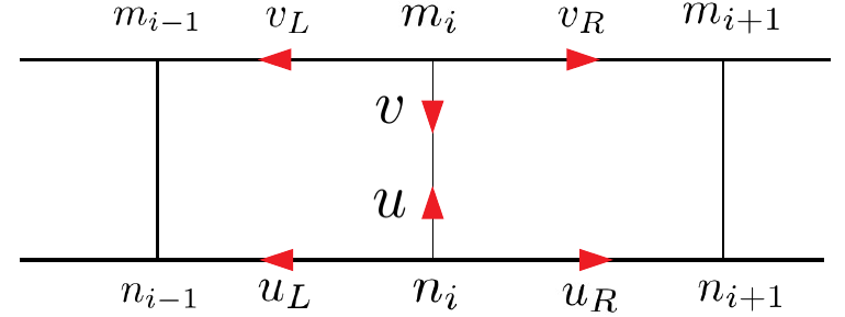
Let us consider a periodic two-leg ladder (see Fig. 3) with sites at each leg are labeled by $i=1,2,\cdots,L$. For both the legs, each site $i$ can be either vacant or it can be occupied by one or more particles: $n_{i}$ particles in the lower leg and $m_{i}$ in the upper leg. We assume that the hop rates depend on the occupation number of the departure site and the corresponding site on the other leg. From any randomly chosen site $i$ of the lower leg, one particle can hop to its right nearest neighbour with rate $u_{R}(n_{i},m_{i})$, left nearest neighbour with rate $u_{L}(n_{i},m_{i})$ and site $i$ of upper leg with rate $u(n_{i},m_{i})$. Similarly for upper leg, one particle from site $i$, can hop to its right and left nearest neighbours with rate $v_{R}(n_{i},m_{i})$ and $v_{L}(n_{i},m_{i})$ respectively and site $i$ of lower leg with rate $v(n_{i},m_{i})$.

Figure 3: Periodic ladder, with two legs, $n_{i}$ and $m_{i}$ are number of particles at site $i$ in the lower and upper leg respectively. A particle from any randomly chosen site $i$ of lower leg, can hop to its right nearest neighbour with rate $u_{R}(n_{i},m_{i})$, left nearest neighbour with rate $u_{L}(n_{i},m_{i})$ and site $i$ of upper leg with rate $u(n_{i},m_{i})$. For upper leg, a particle from site $i$ can hop to its right nearest neighbour with rate $v_{R}(n_{i},m_{i})$, left nearest neighbour with rate $v_{L}(n_{i},m_{i})$ and site $i$ of lower leg with rate $v(n_{i},m_{i})$.

We demand that the model evolves to a FSS

$$P(\{n_{i},m_{i}\})=\frac{1}{Q_{L,N}}\prod_{i=1}^{L}f(n_{i},m_{i})~{}\delta\left(\sum_{i}(n_{i}+m_{i})-N\right)$$ (6)

with a canonical partition function

$$Q_{L,N}=\sum_{\{n_{i}\};\{m_{i}\}}\prod_{i=1}^{L}f(n_{i},m_{i})~{}\delta\left(\sum_{i}(n_{i}+m_{i})-N\right).$$ (7)

The total number of particles $N=\sum_{i=1}^{L}(m_{i}+n_{i})$ and thus the density of the system $\rho=\frac{N}{2L}$ is conserved by the dynamics. FSS as in Eq. (6) can be obtained using - (a) DB, when $u_{R}(n,m)=u_{L}(n,m)=\alpha u(n,m)$, $v_{R}(n,m)=v_{L}(n,m)=\beta v(n,m)$, $\alpha$ and $\beta$ are two different constants. (b) PWB, when the rates $u_{R}(n,m)=\alpha u(n,m)$, $u_{L}(n,m)=\beta u(n,m)$, $v_{R}(n,m)=\gamma v(n,m)$ and $v_{L}(n,m)=\delta v(n,m)$ where $\alpha$, $\beta$, $\gamma$ and $\delta$ are four different constants, i.e, the ratios of the rates are independent of $n$ and $m$. The steady state weight in both the cases is defined by $f(n.m)=\prod_{i=1}^{n}[u(i,m)]^{-1}\prod_{j=1}^{m}[v(0,j)]^{-1}$. Our aim is to find whether such a FSS is possible when rate functions in all hopping directions are different. To answer this question, we employ the MB condition described in Eq. (1).
(i) Let us consider a configuration $C\equiv\{\cdots,n_{i-1},m_{i-1},n_{i},m_{i},n_{i+1},m_{i+1}\cdots\}$. Fluxes generated by particle hopping from site $i$ of lower leg, to its right and left nearest neighbours of this configuration $C$, can be balanced with the flux obtained by a particle hopping from site $i$ in the upper leg of another configuration $C^{\prime}\equiv\{\cdots,n_{i-1},m_{i-1},n_{i}-1,m_{i}+1,n_{i+1},m_{i+1}\cdots\}$ to site $i$ of the lower leg. The flux balance scheme in Eq. (1) gives the following equation

$$v(n_{i}-1,m_{i}+1)~{}P(\cdots,n_{i-1},m_{i-1},n_{i}-1,m_{i}+1,n_{i+1},m_{i+1}\cdots)$$ (8)

$$=[~{}u_{R}(n_{i},m_{i})+u_{L}(n_{i},m_{i})~{}]~{}P(\cdots,n_{i-1},m_{i-1},n_{i},m_{i},n_{i+1},m_{i+1}\cdots).$$ (9)

(ii) Similarly, fluxes generated by a particle hopping from site $i$ of upper leg to its right and left nearest neighbours of the configuration $C$, can be balanced with the flux obtained by a particle hopping from site $i$ in the lower leg of another configuration $C^{\prime\prime}\equiv\{\cdots,n_{i-1},m_{i-1},n_{i}+1,m_{i}-1,n_{i+1},m_{i+1}\cdots\}$ to site $i$ of the upper leg. Then, the flux balance scheme in Eq. (1) gives the following equation

$$u(n_{i}+1,m_{i}-1)~{}P(\cdots,n_{i-1},m_{i-1},n_{i}+1,m_{i}-1,n_{i+1},m_{i+1}\cdots)$$ (10)

$$=[~{}v_{R}(n_{i},m_{i})+v_{L}(n_{i},m_{i})~{}]~{}P(\cdots,n_{i-1},m_{i-1},n_{i},m_{i},n_{i+1},m_{i+1}\cdots).$$ (11)

One can verify that a factorized form of steady state, as in Eq. (6), is indeed possible when the hop rates at site $i$ satisfy the following conditions

$$[~{}u_{R}(n_{i},m_{i})+u_{L}(n_{i},m_{i})~{}]=u(n_{i},m_{i})=\frac{f(n_{i}-1,m_{i})}{f(n_{i},m_{i})},$$ (12)

$$[~{}v_{R}(n_{i},m_{i})+v_{L}(n_{i},m_{i})~{}]=v(n_{i},m_{i})=\frac{f(n_{i},m_{i}-1)}{f(n_{i},m_{i})}$$ (13)

and the steady state weight is defined as

$$f(n,m)=\prod_{i=1}^{n}[u(i,m)]^{-1}\prod_{j=1}^{m}[v(0,j)]^{-1}.$$ (14)

3.1 Calculation of current

One can show following Eqs. (12) and (13) that this particle hopping model on a ladder has a FSS when the asymmetric rate functions satisfy the following distinct functional forms

$$u_{R}(n,m)=u(n,m)~{}[1-\delta+\gamma u(n-1,m)]~{}{\rm;}~{}u_{L}(n,m)=u(n,m)~{}[\delta-\gamma u(n-1,m)],$$ (15)

$$v_{R}(n,m)=v(n,m)~{}[\delta^{\prime}-\gamma^{\prime}v(n,m-1)]~{}{\rm;}~{}v_{L}(n,m)=v(n,m)~{}[1-\delta^{\prime}+\gamma^{\prime}v(n,m-1)],$$ (16)

characterized by four independent parameters $0\leq\delta\leq 1$, $0\leq\gamma\leq\delta/u(n,m)|_{max}$ and $0\leq\delta^{\prime}\leq 1$, $0\leq\gamma^{\prime}\leq\delta^{\prime}/v(n,m)|_{max}$. The range of $\delta$, $\gamma$ and $\delta^{\prime}$, $\gamma^{\prime}$ are chosen such that the hop rates $u_{R,L}(n)$ and $v_{R,L}(n)$ remain positive. We consider the rates $u(n,m)$ and $v(n,m)$ as

$$u(n,m)=\frac{mn+n-m+1}{mn+n+2}~{}~{}{\rm and}~{}~{}v(n,m)=\frac{mn+2}{mn+n+2},$$ (18)

which give a simple expression of the steady state weight

$$f(n,m)=\frac{mn+n+2}{2}.$$ (19)

Let us consider the parameters, $\delta=\frac{n+1}{mn-m+n+1}$, $\gamma=\left(\frac{\alpha}{4}\right)^{2}\frac{m+n}{mn-2m+n}$ and $\delta^{\prime}=\frac{mn-n}{mn+2}$, $\gamma^{\prime}=\left(\frac{\alpha-2}{4}\right)\frac{m+n}{mn-n+2}$, following Eqs. (15) and (16), we get

$$u_{R}(n,m)=\frac{mn-m}{mn+n+2}+\left(\frac{\alpha}{4}\right)^{2}\frac{m+n}{mn+n+2},$$ (20)

$$u_{L}(n,m)=\frac{n+1}{mn+n+2}-\left(\frac{\alpha}{4}\right)^{2}\frac{m+n}{mn+n+2},$$ (21)

$$v_{R}(n,m)=\frac{mn-n}{mn+n+2}-\frac{(\alpha-2)(m+n)}{4(mn+n+2)},$$ (22)

$$v_{L}(n,m)=\frac{n+2}{mn+n+2}+\frac{(\alpha-2)(m+n)}{4(mn+n+2)}.$$ (23)

The model parameter $\alpha$ has been taken in the range $[0,4]$ such that all the rates in Eqs. (20) - (23) remain positive. We can express the grand canonical partition function following Eq. (7), $Z_{L}(z)=\sum_{N=0}^{\infty}z^{N}Q_{L,N}=[F(z)]^{L}$ with

$$F(z)=\sum_{n=0}^{\infty}\sum_{m=0}^{\infty}z^{n}z^{m}f(n,m)=\frac{2z^{2}-3z+2}{2(z-1)^{4}},$$ (24)

where the fugacity $z$ controls the particle density through the relation

$$\rho(z)=(z/2)F^{\prime}(z)/F(z)=\frac{z((5-4z)z-5)}{2(z-1)(2+z(2z-3))}.$$ (25)

In a similar way, one can calculate the particle densities in both legs, $\rho_{1}$ in the lower leg and $\rho_{2}$ in the upper leg as

$$\rho_{1}(z)=\frac{z(3z-2z^{2}-3)}{(z-1)(2+z(2z-3))}~{}~{}{\rm and}~{}~{}\rho_{2}(z)=\frac{2z(z-z^{2}-1)}{(z-1)(2+z(2z-3))}.$$ (26)

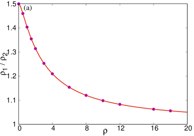
Note that the densities $\rho$, $\rho_{1}$ and $\rho_{2}$ in Eqs. (25) and (26) do not depend on $\alpha$; i.e, for any value of $\alpha$, a given $z$ corresponds to a unique density $\rho$. At $z\rightarrow 0$ (i.e, $\rho\rightarrow 0$), both the densities $\rho_{1}\rightarrow 0$ and $\rho_{2}\rightarrow 0$ but their ratio remains finite, $\frac{3}{2}$. Similarly for $z\rightarrow 1$ (i.e, $\rho\rightarrow\infty$), both $\rho_{1}\rightarrow\infty$ and $\rho_{2}\rightarrow\infty$ but the ratio becomes $1$. The relative particle density $\frac{\rho_{1}}{\rho_{2}}$ as a function of the total density of the system $\rho$ has been shown in Fig. 4(a). We can calculate the currents in both legs, $J_{1}$ for lower leg and $J_{2}$ for upper leg as

$$J_{1}=\frac{1}{F(z)}\sum_{n=1}^{\infty}\sum_{m=0}^{\infty}~{}[u_{r}(n,m)-u_{l}(n,m)]~{}z^{n+m}f(n,m)=\frac{z(z(24-z\alpha^{2})+\alpha^{2}-16)}{4(4z^{2}-6z+4)},$$ (27)

$$J_{2}=\frac{1}{F(z)}\sum_{n=0}^{\infty}\sum_{m=1}^{\infty}~{}[v_{r}(n,m)-v_{l}(n,m)]~{}z^{n+m}f(n,m)=\frac{z(z(6+z(\alpha-2))-\alpha-2)}{4z^{2}-6z+4}$$ (28)

(29)

and the total current can be expressed as

$$J=J_{1}+J_{2}=\frac{z((\alpha-2)^{2}(1-z^{2})-4(z^{2}-12z+7))}{4(4z^{2}-6z+4)}.$$ (30)

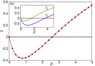
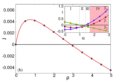
Figure 4: (a) Relative particle density $\frac{\rho_{1}}{\rho_{2}}$ as a function of density $\rho$, measured from simulation (points) on a system of size $L=100$, is compared with exact expressions of $\rho_{1}$ and $\rho_{2}$ as in Eq. (26). (b) The total current $J$ as a function of density $\rho$ for $\alpha=0.6$. The total current reverses its direction at $\rho=2.611$. The inset shows currents $J_{1,2}$ as a function of $\rho$ for $\alpha=0.6$. Points are from simulations with $L=100$ and averaged over $10^{8}$ trajectories, solid lines are exact according to Eqs. (27) - (30).

For $z\rightarrow 1$, the density $\rho\rightarrow\infty$ and the total current $J$ turns out to be $J=2$. For $z\rightarrow 0$, i.e, when $\rho\rightarrow 0$, the total current $J$ vanishes. Infact there exists a line in $\rho$ - $\alpha$ parameter space, where the total current $J$ also vanishes. This line can be expressed following Eq. (30) as

$$z^{*}=\frac{24-\sqrt{(\alpha-2)^{4}-24(\alpha-2)^{2}+464}}{(\alpha-2)^{2}+4}$$ (31)

where, $z^{*}$ is the fugacity. Since $z^{*}$ corresponds to a unique density $\rho^{*}=\rho(z^{*})$, $J=0$ line can also be expressed in terms of the density $\rho^{*}$ as a function of $\alpha$ as

$$\rho^{*}=1-\frac{\kappa^{2}}{8}+\frac{\sqrt{\kappa^{4}-24\kappa^{2}+464}}{8}+\frac{16(\kappa^{2}-12)-96\sqrt{\kappa^{4}-24\kappa^{2}+464}}{3312+7\kappa^{2}(\kappa^{2}-24)}$$ (32)

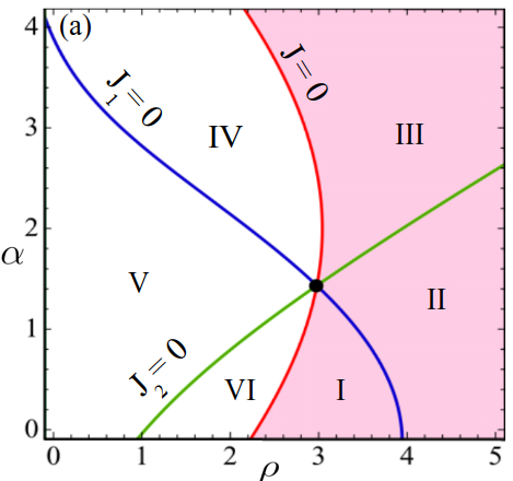
where $\kappa=(\alpha-2)$. Note that $\rho^{*}$ corresponds to the value of density at which the total current $J$ reverses its direction. $\rho^{*}$ as a function of $\alpha$ is shown in Fig. 5(a) and marked as $J=0$ line (the red one). As expected, $\rho^{*}$ as a function of $\alpha$ is symmetric about $\alpha=2$ and has a maximum at $\alpha=2$. Corresponding densities for $\alpha=0$ and $4$ are $\rho_{1}^{*}=(\frac{39}{86}+\frac{31\sqrt{6}}{43})\approx 2.219$ and at $\alpha=2$ the density becomes $\rho_{2}^{*}=(\frac{65}{69}+\frac{53\sqrt{29}}{138})\approx 3.01$. For $\alpha=0.6$, the total current $J$ reverses its direction, following Eq. (32), at $\rho=2.611$ which is shown in Fig. 4(b).

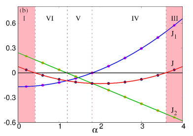
Figure 5: (a) Different regions in $\rho$ - $\alpha$ plane corresponding the direction of flow of the currents $J_{1,2}$ and $J$. Three lines $J=0$, $J_{1}=0$ and $J_{2}=0$ separate this plane in six regions. In the shaded regions I ($J_{1}<0$, $J_{2}>0$ and $J_{2}>|J_{1}|$), II ($J_{1}>0$ and $J_{2}>0$) and III ($J_{1}>0$, $J_{2}<0$ and $J_{1}>|J_{2}|$), total current $J$ flows towards right. Similarly the current $J$ flows towards left in the regions IV ($J_{1}>0$, $J_{2}<0$ and $|J_{2}|>J_{1}$), V ($J_{1}<0$ and $J_{2}<0$) and VI ($J_{1}<0$, $J_{2}>0$ and $|J_{1}|>J_{2}$), (b) $J_{1,2}$ and $J$ as a function of $\alpha$ for $\rho=2.5$. Five different regions are visible at $\rho=2.5$, the total current $J$ exhibits a re-entrance. For $\alpha<0.411$, $J$ is positive, the direction of $J$ is reversed with the increase of $\alpha$ (regions separated by dashed lines). Further for $\alpha>3.589$, $J$ re-enters to the regime of forward flow. Regions marked here carry the same information as in (a). Points are from simulations with $L=100$ and averaged over $10^{8}$ trajectories, solid lines are exact according to Eqs. (27) - (30).

In the $\rho$ - $\alpha$ plane, we have shown the three lines of separations, $J_{1}=0,J_{2}=0,J=0;$ corresponding currents flip their direction when these lines are crossed by varying the density $\rho$ or the parameter $\alpha.$ In the shaded region of Fig. 5(a), the total current $J$ flows towards right. This is possible when I. $J_{1}<0$, $J_{2}>0$ and $J_{2}>|J_{1}|$ or II. when both $J_{1}>0$ and $J_{2}>0$ or III. when $J_{1}>0$, $J_{2}<0$ and $J_{1}>|J_{2}|.$ Similarly when total current $J$ flows towards left, we have three more regions IV. $J_{1}>0$, $J_{2}<0$ and $|J_{2}|>J_{1}$ , V. both $J_{1}<0$ and $J_{2}<0$ and VI. $J_{1}<0$, $J_{2}>0$ and $|J_{1}|>J_{2}$. All these regions are marked in Fig. 5(a). It is evident from the figure that one can access at most four regions by changing $\rho$ for a fixed $\alpha$, whereas at most five regions can be accessed by changing $\alpha$ for a fixed $\rho$. The total current $J$, when $\rho$ is varied, does not exhibit re-entrance, whereas it shows re-entrance when $\alpha$ is varied in a certain zone. This re-entrance of the total current $J$ as a function of $\alpha$ occurs in the density region $\rho_{1}^{*}<\rho<\rho_{2}^{*}$. In Fig. 5(b) we have plotted $J_{1,2}$ and $J$ as a function of $\alpha$ keeping the particle density fixed at $\rho=2.5;$ five different regions are clearly visible. At $\alpha=0$, $J_{1}$ is negative, $J_{2}$ is positive and $J_{2}>|J_{1}|$. Thus at $\alpha=0$ and for small $\alpha$, the total current $J=J_{1}+J_{2}$ is positive. Note that, $\frac{dJ_{1}}{d\alpha}>0$ and $\frac{dJ_{2}}{d\alpha}<0$ following Eqs. (27) and (29). Since, $J_{1}$ increases faster than $J_{2}$, it is evident that for larger $\alpha$ we may get the total current $J$ positive again. Infact, the total current $J$ vanishes at $\alpha=0.411$ and then the direction of the total current is reversed. Further increase of $\alpha$ keeps the direction of the total current unaltered until $\alpha=3.589,$ where $J$ vanishes and then reverses its direction again, re-entering to regime of forward-flow and exhibits the re-entrance.

4 Two-leg ladder with pair factorized steady state

When the steady state is factorized as a product of two site clusters, it is commonly known as pair factorized steady state (PFSS). It was proposed and studied in [24], where it was shown that for a particular class of PFSS, the system under consideration exhibits a condensation transition. Later PFSS has been found in continuous mass-transfer models [25, 26], in systems with open boundaries [27] and in random graphs [28], etc. In our ladder example, we assume that the system evolves to the PFSS which looks like

$$P(\{n_{i},m_{i}\})=\frac{1}{Q_{L,N}}\prod_{i=1}^{L}g(n_{i},m_{i},n_{i+1},m_{i+1})~{}\delta\left(\sum_{i}(n_{i}+m_{i})-N\right)$$ (33)

with a canonical partition function

$$Q_{L,N}=\sum_{\{n_{i}\};\{m_{i}\}}\prod_{i=1}^{L}g(n_{i},m_{i},n_{i+1},m_{i+1})~{}\delta\left(\sum_{i}(n_{i}+m_{i})-N\right).$$ (34)

If the hop rate depends only on the occupation number of the departure site and the corresponding site on the other leg, PFSS as in Eq. (33) is not possible in general. We generalize that the hop rates now depend not only on the occupation number of departure site, also on the occupation numbers of its two nearest neighbours on both legs, i.e, $u\equiv u(n_{i-1},m_{i-1},n_{i},m_{i},n_{i+1},m_{i+1})$. Here also we ask if such a pair factorized form of steady state is possible when all the rate functions are different. We, using similar arguments of MB as described for FSS, find that a pair factorized form of steady state (PFSS) as in Eq. (33) is possible for the two-leg ladder when the hop rates satisfy

$$[~{}u_{R}(n_{i-1},m_{i-1},n_{i},m_{i},n_{i+1},m_{i+1})+u_{L}(n_{i-1},m_{i-1},n_{i},m_{i},n_{i+1},m_{i+1})~{}]$$ (35)

$$=u(n_{i-1},m_{i-1},n_{i},m_{i},n_{i+1},m_{i+1})=\frac{g(n_{i-1},m_{i-1},n_{i}-1,m_{i})}{g(n_{i-1},m_{i-1},n_{i},m_{i})}\frac{g(n_{i}-1,m_{i},n_{i+1},m_{i+1})}{g(n_{i},m_{i},n_{i+1},m_{i+1})},$$ (36)

(37)

$$[~{}v_{R}(n_{i-1},m_{i-1},n_{i},m_{i},n_{i+1},m_{i+1})+v_{L}(n_{i-1},m_{i-1},n_{i},m_{i},n_{i+1},m_{i+1})~{}]$$ (38)

$$=v(n_{i-1},m_{i-1},n_{i},m_{i},n_{i+1},m_{i+1})=\frac{g(n_{i-1},m_{i-1},n_{i},m_{i}-1)}{g(n_{i-1},m_{i-1},n_{i},m_{i})}\frac{g(n_{i},m_{i}-1,n_{i+1},m_{i+1})}{g(n_{i},m_{i},n_{i+1},m_{i+1})}.$$ (39)

(40)

Let us consider that the weight function $g(n_{i},n_{i+1},m_{i},m_{i+1})$ can be written as the inner product of two 2-dimensional vectors [19]

$$g(n_{i},n_{i+1},m_{i},m_{i+1})=\langle\alpha(n_{i},m_{i})|\beta(n_{i+1},m_{i+1})\rangle$$ (41)

In the grand canonical ensemble where the fugacity $z$ controls the density $\rho$, the partition sum can be written as $Z_{L}(z)=\sum_{N=0}^{\infty}Q_{L,N}z^{N}=\Tr[T(z)^{L}]$ with

$$T(z)=\sum_{n=0}^{\infty}\sum_{m=0}^{\infty}z^{n}z^{m}|\beta(n,m)\rangle\langle\alpha(n,m)|.$$ (42)

We consider a simple 2-dimensional representation by taking,

$$\langle\alpha(n,m)|=((n+1)^{-\nu}(m+1)^{-\nu},(m+1)^{-\nu}),$$ (43)

$$\langle\beta(n,m)|=((n+1)^{1-\nu},(n+1)^{1-\nu}(m+1)^{1-\nu}).$$ (44)

The weight function $g(n_{i},n_{i+1},m_{i},m_{i+1})$ can be determined for the above choice of representation following Eq. (41). The transfer matrix $T(z)$, following Eq. (42), becomes

$$T(z)=\frac{1}{z^{2}}\left(\begin{array}[]{cc}Li_{\nu}(z)Li_{2\nu-1}(z)&Li_{\nu-1}(z)Li_{\nu}(z)\\ (Li_{2\nu-1}(z))^{2}&Li_{\nu-1}(z)Li_{2\nu-1}(z)\end{array}\right),$$ (45)

where $Li_{\nu}(z)$ is the Polylogarithm function defined by $Li_{\nu}(z)=\sum_{n=1}^{\infty}\frac{z^{n}}{n^{\nu}}$. The eigenvalues of $T(z)$ are

$$\lambda_{+}=\frac{1}{z^{2}}(Li_{\nu}(z)+Li_{\nu-1}(z))Li_{2\nu-1}(z)~{}~{}{\rm and}~{}~{}\lambda_{-}=0.$$ (46)

The partition function $Z_{L}(z)$ in the thermodynamic limit becomes $Z_{L}(z)\simeq\lambda_{+}(z)^{L}$ which leads to the density fugacity relation

$$\rho(z)=(z/2)\frac{\partial}{\partial z}\ln(\lambda_{+}(z))=\frac{Li_{\nu-2}(z)+Li_{\nu-1}(z)}{2(Li_{\nu-1}(z)+Li_{\nu}(z))}+\frac{Li_{2\nu-2}(z)}{2Li_{2\nu-1}(z)}-1$$ (47)

and the critical density $\rho_{c}=\lim_{z\rightarrow 1}\rho(z)$. The hop rates $u(n_{i-1},m_{i-1},n_{i},m_{i},n_{i+1},m_{i+1})$ and $v(n_{i-1},m_{i-1},n_{i},m_{i},n_{i+1},m_{i+1})$ can be determined following Eq. (44) as

$$u(n_{i-1},m_{i-1},n_{i},m_{i},n_{i+1},m_{i+1})=\left(\frac{n_{i}}{n_{i}+1}\right)^{1-2\nu}\frac{n_{i}^{\nu}(1+m_{i+1})+(1+m_{i+1})^{\nu}}{(1+m_{i+1})^{\nu}+(1+m_{i+1})(1+n_{i})^{\nu}},$$ (48)

$$v(n_{i-1},m_{i-1},n_{i},m_{i},n_{i+1},m_{i+1})=\left(\frac{m_{i}}{m_{i}+1}\right)^{-2\nu}\frac{m_{i}^{\nu}+m_{i}(1+n_{i-1})^{\nu}}{(1+m_{i})^{\nu}+(1+m_{i})(1+n_{i-1})^{\nu}}.$$ (49)

We consider the rates in the horizontal directions

$$u_{R,L}(n_{i-1},m_{i-1},n_{i},m_{i},n_{i+1},m_{i+1})=(u(n_{i-1},m_{i-1},n_{i},m_{i},n_{i+1},m_{i+1})\pm(\alpha^{2}/2-1))/2,$$ (50)

(51)

$$v_{R,L}(n_{i-1},m_{i-1},n_{i},m_{i},n_{i+1},m_{i+1})=(v(n_{i-1},m_{i-1},n_{i},m_{i},n_{i+1},m_{i+1})\pm(1-\alpha))/2,$$ (52)

where in Eqs. (51) and (52), $u_{R}$ and $v_{R}$ corresponds to ${}^{\prime}+^{\prime}$ sign and $u_{L}$ and $v_{L}$ corresponds to ${}^{\prime}-^{\prime}$ sign, such that they satisfy the conditions in Eqs. (37) and (40). One can verify, following Eqs. (37) and (40) that the average hop rates along the vertical direction become equal for both lower and upper leg as

$$\langle u(n_{i-1},m_{i-1},n_{i},m_{i},n_{i+1},m_{i+1})\rangle=\langle v(n_{i-1},m_{i-1},n_{i},m_{i},n_{i+1},m_{i+1})\rangle=z.$$ (53)

We can explicitly calculate the current $J_{1}$ in the lower leg and $J_{2}$ in the upper leg as

$$J_{1}=\langle u_{R}(.)-u_{L}(.)\rangle=(\alpha^{2}/2-1)~{}\left(1-\frac{Tr[~{}T(z)^{L-1}~{}T_{1}(z)~{}]}{Tr(T(z))^{L}}\right)$$ (54)

$$~{}~{}~{}~{}=(\alpha^{2}/2-1)\left(1-\frac{z~{}[~{}Li_{\nu}(z)+Li_{2\nu-1}(z)~{}]}{[~{}Li_{\nu}(z)+Li_{\nu-1}(z)~{}]~{}Li_{2\nu-1}(z)}\right),$$ (55)

$$J_{2}=\langle v_{R}(.)-v_{L}(.)\rangle=(1-\alpha)~{}\left(1-\frac{Tr[~{}T(z)^{L-1}~{}T_{2}(z)~{}]}{Tr(T(z))^{L}}\right)$$ (56)

$$~{}~{}~{}~{}=(1-\alpha)\left(1-\frac{z~{}[~{}Li_{\nu-1}(z)+Li_{2\nu-1}(z)~{}]}{[~{}Li_{\nu}(z)+Li_{\nu-1}(z)~{}]~{}Li_{2\nu-1}(z)}\right),$$ (57)

where the matrices

$$T_{1}(z)=\frac{1}{z}\left(\begin{array}[]{cc}Li_{\nu}(z)&Li_{\nu}(z)\\ Li_{2\nu-1}(z)&Li_{2\nu-1}(z)\end{array}\right)~{}~{}{\rm and}~{}~{}T_{2}(z)=\frac{1}{z}\left(\begin{array}[]{cc}Li_{2\nu-1}(z)&Li_{\nu-1}(z)\\ Li_{2\nu-1}(z)&Li_{\nu-1}(z)\end{array}\right).$$ (58)

The total current of the system is $J=J_{1}+J_{2}.$

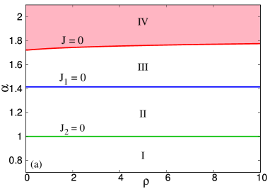
Figure 6: (a) Different regions in $\rho$ - $\alpha$ plane corresponding the direction of flow of the currents $J_{1,2}$ and $J$ for $\nu=1$. Three lines $J=0$, $J_{1}=0$ and $J_{2}=0$ separate this plane in four regions. In the shaded region IV ($J_{1}>0$, $J_{2}<0$ and $J_{1}>|J_{2}|$), the total current $J$ flows towards right. Similarly the total current flows towards left in the regions I ($J_{1}<0$, $J_{2}>0$ and $|J_{1}|>J_{2}$), II ($J_{1}<0$ and $J_{2}<0$) and III ($J_{1}>0$, $J_{2}<0$ and $|J_{2}|>J_{1}$). (b) The total current $J$ as a function of density $\rho$ for $\alpha=1.75$. The total current reverses its direction at density $\rho=2.923$. Inset shows $J_{1,2}$ and $J$ as a function of $\alpha$ for $\nu=1$ and $\rho=0.5$. All four regions are visible at $\rho=0.5$. For small $\alpha$ , $J<0$ and the direction is reversed for $\alpha>1.725$. Regions, separated by dashed lines, carry the same information as in figure (a). Points are from simulations with $L=100$ and averaged over $10^{8}$ trajectories, solid lines are exact according to Eqs. (55) - (57).

We consider a particular case, when $\nu=1$. In the $\rho$ - $\alpha$ plane, we have shown the three lines of separations, $J_{1}=0,J_{2}=0,J=0;$ corresponding currents flip their direction when these lines are crossed by varying the density $\rho$ or the parameter $\alpha.$ In the shaded region (IV) of Fig 6 (a), the total current $J$ flows towards right. For our choices of rates, this is possible only when $J_{1}>0$, $J_{2}<0$ and $J_{1}>|J_{2}|.$ Similarly when the total current $J$ flows towards left, we have three more regions I. $J_{1}<0$, $J_{2}>0$ and $|J_{1}|>J_{2}$, II. both $J_{1}<0$ and $J_{2}<0$ and III. $J_{1}>0$, $J_{2}<0$ and $|J_{2}|>J_{1}$. All these regions are marked in Fig. 6(a). One can access at most two regions by changing $\rho$ for a fixed $\alpha$ (region IV to III), whereas all four regions can be accessed by changing $\alpha$ for a fixed $\rho.$ It is evident from Fig. 6(a) that the total current $J$ as a function of density $\rho$ reverses its direction in a certain zone. This current reversal occurs in the region $1.72<\alpha\leq 1.78$. For $\alpha=1.75$, direction of the total current $J$ is reversed at $\rho\approx 2.923$, which is shown in Fig. 6(b). In the inset of Fig. 6(b), $J_{1,2}$ and $J$ have been plotted as a function of $\alpha$ for a fixed particle density at $\rho=0.5;$ all four regions are clearly visible here. For small $\alpha$, $J$ is negative and vanishes at $\alpha=1.725$ then the direction of the current is reversed. Further increase of $\alpha$ keeps $J$ in this same direction.

5 Multibalance in other nonequilibrium lattice models

Multibalance condition that we introduced is very useful in solving nonequilibrium problems. A few examples are given below.

5.1 Asymmetric finite range process (AFRP) with nearest neighbour and next nearest neighbour hopping

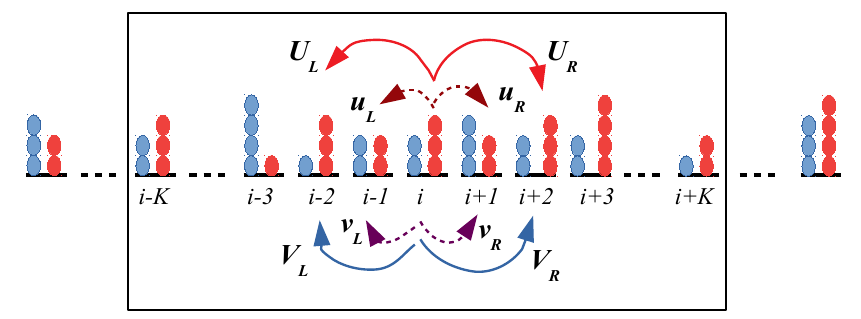
Let us consider a system of $N$ particles on a one dimensional periodic lattice with $L$ sites labeled by $i=1,2,\cdots,L$ (see Fig. 7). Each site $i$ can accommodate $n_{i}\geq 0$ number of particles. From a randomly chosen site $i$, one particle can hop to its right nearest neighbour with rate $u_{R}(.)$, left nearest neighbour with rate $u_{L}(.)$ and as well as to the next nearest neighbours with rates $U_{R}(.)$ for right, $U_{L}(.)$ for left. All these rates depend on the number of particles at all the sites within a range $K$ w.r.t the departure site [19, 20].

Figure 7: FRP in one dimension where one particle hops from a site $i$ to its left and right neighbours with rates $u_{L}(.)$ and $u_{R}(.)$ and left and right next nearest neighbours with rates $U_{L}(.)$ and $U_{R}(.)$. All these rates depend on occupation of site $i$ (here $n_{i}=3$) and all its neighbours within a range $K$.

We assume that the system evolves to a cluster factorized steady state

$$P(\{n_{i}\})\propto\prod_{i=1}^{L}g(n_{i},n_{i+1},\cdots n_{i+K})~{}\delta\left(\sum_{i}n_{i}-N\right).$$ (59)

$N$ is the total number of particles and $\rho=\frac{N}{L}$ is conserved by the dynamics. We now ask, if such a cluster factorized form of steady state is possible when the rates in all four directions are different i.e the ratios of rates are not independent of $n$. We can say that steady state as in Eq. (59) can be obtained using MB for a given function $u(n_{i-K},\cdots,n_{i},\cdots n_{i+K})$, when the hop rates satisfy $u_{R}(n_{i-K},\cdots,n_{i},\cdots n_{i+K})=u_{L}(n_{i-K},\cdots,n_{i},\cdots n_{i+K})=u(n_{i-K},\cdots,n_{i},\cdots n_{i+K})$ and

$$U_{R}(n_{i-K},\cdots,n_{i},\cdots n_{i+K})+U_{L}(n_{i-K},\cdots,n_{i},\cdots n_{i+K})$$ (60)

$$=u(n_{i-K},\cdots,n_{i},\cdots n_{i+K})=\prod_{k=1}^{K}\frac{g(\widetilde{n}_{i-K+k},\widetilde{n}_{i-K+1+k},\cdots,\widetilde{n}_{i+k})}{g(n_{i-K+k},n_{i-K+1+k},\cdots,n_{i+k})},$$ (61)

where $\widetilde{n}_{j}=n_{j}-\delta_{ji}$.

5.2 Two species FRP with directional asymmetry

We consider a one dimensional periodic lattice (see Fig. 8) with sites labeled by $i=1,2,\cdots,L$. At each site $i$, there are $n_{i}$ particles of species $A$ (coloured red) and $m_{i}$ particles of species $B$ (coloured blue). From a randomly chosen site $i$, a particle of species $A$, can hop to its right and left nearest neighbours with rates $u_{R}(.)$ and $u_{L}(.)$, it can hop to right and left next nearest neighbours with rates $U_{R}(.)$ and $U_{L}(.)$.

Figure 8: Two species asymmetric FRP model in one dimension. A particle of species A (coloured red) can hop to its right and left nearest neighbours with rates $u_{R}(.)$ and $u_{L}(.)$, to right and left next nearest neighbours with rates $U_{R}(.)$ and $U_{L}(.)$. Similarly, particle of species $B$ (coloured blue), can hop to its right and left nearest neighbours with rates $v_{R}(.)$ and $v_{L}(.)$, to right and left next nearest neighbours with rates $V_{R}(.)$ and $V_{L}(.)$.

Similarly, a particle of species $B$, can hop to its right and left nearest neighbours with rates $v_{R}(.)$ and $v_{L}(.)$, to right and left next nearest neighbours with rates $V_{R}(.)$ and $V_{L}(.)$. All these rates depend on the number of particles of both species at the departure site and its two nearest neighbours. We demand that this model evolves to a PFSS

$$P(\{n_{i},m_{i}\})\propto\prod_{i=1}^{L}g(n_{i},m_{i},n_{i+1},m_{i+1})~{}\delta\left(\sum_{i}n_{i}-N\right)\delta\left(\sum_{i}m_{i}-M\right),$$ (62)

where, $N$ is total number of particles of species $A$ and $M$ is total number of particles of species $B$. Such a PFSS as in Eq. (62) can be obtained using MB for the given functions of $u(n_{i-1},m_{i-1},n_{i},m_{i},n_{i+1},m_{i+1})$ and $v(n_{i-1},m_{i-1},n_{i},m_{i},n_{i+1},m_{i+1})$, when the hop rates of species $A$ satisfy $u_{R}(n_{i-1},m_{i-1},n_{i},m_{i},n_{i+1},m_{i+1})=u_{L}(n_{i-1},m_{i-1},n_{i},m_{i},n_{i+1},m_{i+1})=u(n_{i-1},m_{i-1},n_{i},m_{i},n_{i+1},m_{i+1})$ and

$$\left[~{}U_{R}(n_{i-1},m_{i-1},n_{i},m_{i},n_{i+1},m_{i+1})+U_{L}(n_{i-1},m_{i-1},n_{i},m_{i},n_{i+1},m_{i+1})~{}\right]$$ (63)

$$=u(n_{i-1},m_{i-1},n_{i},m_{i},n_{i+1},m_{i+1})=\frac{g(n_{i-1},m_{i-1},n_{i}-1,m_{i})}{g(n_{i-1},m_{i-1},n_{i},m_{i})}\frac{g(n_{i}-1,m_{i},n_{i+1},m_{i+1})}{g(n_{i},m_{i},n_{i+1},m_{i+1})},$$ (64)

(65)

similarly, the hop rates of species $B$ satisfy $v_{R}(n_{i-1},m_{i-1},n_{i},m_{i},n_{i+1},m_{i+1})=v_{L}(n_{i-1},m_{i-1},n_{i},m_{i},n_{i+1},m_{i+1})=v(n_{i-1},m_{i-1},n_{i},m_{i},n_{i+1},m_{i+1})$ and

$$\left[~{}V_{R}(n_{i-1},m_{i-1},n_{i},m_{i},n_{i+1},m_{i+1})+V_{L}(n_{i-1},m_{i-1},n_{i},m_{i},n_{i+1},m_{i+1})~{}\right]$$ (66)

$$=v(n_{i-1},m_{i-1},n_{i},m_{i},n_{i+1},m_{i+1})=\frac{g(n_{i-1},m_{i-1},n_{i},m_{i}-1)}{g(n_{i-1},m_{i-1},n_{i},m_{i})}\frac{g(n_{i},m_{i}-1,n_{i+1},m_{i+1})}{g(n_{i},m_{i},n_{i+1},m_{i+1})}.$$ (67)

(68)

6 Summary

The steady states of non-equilibrium systems are very much dependent on the complexity of the dynamics and it is difficult to track down a systematic procedure to obtain the steady state measure of a system with a given dynamics. In this regard, starting from the master equation that governs the time evolution of a many particle system in the configuration space, several flux cancellation schemes have been in use for obtaining the exact steady state weight. These schemes include matrix product ansatz (MPA) [14], h-balance scheme [20] and pairwise balance condition (PWB). In this article we introduced a new kind of balance condition, namely multibalance (MB), where the sum of incoming fluxes from a set of configurations to any configuration $C$ is balanced by the total outgoing flux to set of configurations chosen suitably.

We have applied the MB condition to a class of nonequilibrium lattice models. We have given an example of the asymmetric ZRP in two dimensions and discussed that a factorized steady state (FSS) can be obtained using MB with specific conditions on hop rates. We have considered an interesting model, particle hopping on a ladder, where a particle from a randomly chosen site in one leg, can hop to its two nearest neighbours and also to that site of the other leg. We first assumed that the model evolves to FSS and discussed the cases of obtaining FSS using detailed balance (DB) and PWB, which are well known. We ask that such a FSS is possible at all when hop rates in all directions are different. In this situation, MB can be employed to solve this model exactly to obtain the FSS with specific conditions on the hop rates. We have calculated currents generated by both legs and also the total current for this model. It is shown that the total current flows in same direction in two different regions separated by an intermediate region, where it flows in the opposite direction. To explain this behaviour, we have mentioned it clearly that total current being positive or negative does not always mean that currents on both legs are individually positive or negative.

We extended the model of particle hopping on ladder beyond FSS; we have discussed that pair factorized form of steady state (PFSS) can also be obtained using MB if the hop rates satisfy some other conditions.

The problem which we studied here, can also be mapped to hopping of particles on a periodic lattice, where each particle has two internal degrees of freedom $\sigma=\pm$ that replace the two legs of the ladder. Then $(n_{i},m_{i})$ translates to $(n^{+}_{i},n^{-}_{i}).$ In this model, a particle from site $i$ can hop to its right and left nearest neighbour with rate $u_{R,\sigma}(n^{+}_{i},n^{-}_{i})$ and $u_{L,\sigma}(n^{+}_{i},n^{-}_{i})$ or it can change it’s internal degree of freedom $\sigma\to-\sigma$ with rate $u_{\sigma}(n^{+}_{i},n^{-}_{i})$, which violates the conservation of particles of each kind. $J_{\pm}\equiv J_{1,2}$ are the currents generated by each kind of particles and $J$ is the sum of $J_{+}$ and $J_{-}.$

To emphasize the utility and the strength of the MB condition introduced here, we have discussed a few examples of nonequilibrium lattice models where we can obtain steady state using MB. For the asymmetric finite range process, with nearest and next nearest neighbours hopping, cluster factorized form of steady state (CFSS) can be obtained using MB for certain conditions on hop rates, which helps us calculating the steady state average of the observable using Transfer Matrix method introduced earlier [19]. In another interesting example, we have considered a two species FRP with directional asymmetry, and with nearest neighbours and next nearest neighbours hopping. PFSS can be obtained for this model under specific conditions on hop rates.

In summary, we introduced a new kind of flux balance condition, namely MB, to obtain steady state weights of nonequilibrium systems and demonstrate its utility in many different kinds of non-equilibrium dynamics, including those where the interactions extend beyond two sites. We believe that the MB technique will be very helpful in finding steady states of many other nonequilibrium systems.

Appendix

In this Appendix, we study ZRP in two dimensions and obtain a condition on hop rates so that the steady state is factorized. We write the master equation of ZRP in a periodic two dimensional lattice of size $(L\times L)$, sites $(i,j)$ with $i=1,2,3\cdots L$, $j=1,2,3,\cdots L$ and denote the configurations in terms of the site variables $\{n_{i,j}\}$

$$\frac{d}{dt}P(\{n_{i,j}\})=\sum_{i=1}^{L}\sum_{j=1}^{L}\left[~{}u_{r}(n_{i-1,j}+1)P(\dots n_{i-1,j}+1,n_{i,j}-1\dots)\right.$$ (69)

$$\left.\hskip 42.67912pt+u_{l}(n_{i+1,j}+1)P(\dots n_{i,j}-1,n_{i+1,j}+1\dots)\right.$$ (70)

$$\left.\hskip 42.67912pt+u_{u}(n_{i,j-1}+1)P(\dots n_{i,j-1}+1,\dots n_{i,j}-1\dots)\right.$$ (71)

$$\left.\hskip 42.67912pt+u_{d}(n_{i,j+1}+1)P(\dots n_{i,j}-1\dots n_{i,j+1}+1\dots)~{}\right]$$ (72)

$$\hskip 14.22636pt-\sum_{i=1}^{L}\sum_{j=1}^{L}\left[~{}u_{r}(n_{i,j})+u_{l}(n_{i,j})+u_{u}(n_{i,j})+u_{d}(n_{i,j})~{}\right]\,\,P(\{n_{i,j}\})$$ (73)

We will like to see if there can be a FSS which neither satisfies DB nor satisfies PWB. In particular, we want to see if there is a FSS which can be obtained using MB. With a FSS, the steady state master equation for any arbitrary configuration of this two dimensional ZRP model reads as,

$$\begin{array}[]{c}\sum_{i=1}^{L}\sum_{j=1}^{L}\left[~{}u_{r}(n_{i,j})+u_{l}(n_{i,j})+u_{u}(n_{i,j})+u_{d}(n_{i,j})~{}\right]\\ \dots f(n_{i,j-1})\dots f(n_{i-1,j})f(n_{i,j})f(n_{i+1,j})\dots f(n_{i,j+1})\\ -[~{}\,\sum_{i=1}^{L}\sum_{j=1}^{L}u_{r}(n_{i-1,j}+1)\dots f(n_{i-1,j}+1)f(n_{i,j}-1)\dots\cr+\sum_{i=1}^{L}\sum_{j=1}^{L}u_{l}(n_{i+1,j}+1)\dots f(n_{i,j}-1)f(n_{i+1,j}+1)\dots\cr+\sum_{i=1}^{L}\sum_{j=1}^{L}u_{u}(n_{i,j-1}+1)\dots f(n_{i,j-1}+1)\dots f(n_{i,j}-1)\dots\cr+\sum_{i=1}^{L}\sum_{j=1}^{L}u_{d}(n_{i,j+1}+1)\dots f(n_{i,j}-1)\dots f(n_{i,j+1}+1)\dots~{}]=0.\\ \\ \end{array}$$ (74)

One can show following Eq. (LABEL:eq:master_ZRP1) that it is possible to obtain an exact FSS for this model when

$$u_{r}(n)+u_{l}(n)+u_{u}(n)+u_{d}(n)=u(n)$$ (75)

and the steady state is defined as $f(n)=\prod_{\nu=1}^{n}u(\nu)^{-1}$, if the asymmetric rate functions have the following generic functional form

$$u_{r}(n)=(u(n)/2)~{}[\alpha_{1}-\beta_{1}u(n-1)]~{}{\rm;}~{}~{}u_{l}(n)=(u(n)/2)~{}[1-\alpha_{1}+\beta_{1}u(n-1)],$$ (76)

$$u_{u}(n)=(u(n)/2)~{}[\alpha_{2}-\beta_{2}u(n-1)]~{}{\rm;}~{}~{}u_{d}(n)=(u(n)/2)~{}[1-\alpha_{2}+\beta_{2}u(n-1)],$$ (77)

characterized by the independent parameters $0\leq\alpha_{1}\leq 1$, $0\leq\beta_{1}\leq\alpha_{1}/u(n)|_{max}$, $0\leq\alpha_{2}\leq 1$ and $0\leq\beta_{2}\leq\alpha_{2}/u(n)|_{max}$. The range of $\alpha_{1}$, $\beta_{1}$ and $\alpha_{2}$, $\beta_{2}$ are chosen such that the hop rates $u_{r,l,u,d}(n)$ remain positive. Note that Eq. (75) is the most generalized condition on the hop rates to obtain the FSS using MB. The specific choices of hop rates in Eqs. (4) and (5) for the model described in the text also satisfy this generalized condition in Eq. (75).

References

• [1] Schmittmann, B. and Zia, R. K. P., Statistical Mechanics of Driven Diffusive Systems ed. Domb, C. and Lebowitz, J. L., 1995 Academic Press, New York.
• [2] Nonequilibrium Statistical Mechanics In One Dimension, ed. Privman, V., 1997 Cambridge University Press.
• [3] Tolman, R. C. (1938), The Principles of Statistical Mechanics, Oxford University Press, London, UK.
• [4] Boltzmann, L., (1964), Lectures on gas theory, Berkeley, CA, USA: U. of California Press.
• [5] Spitzer, F., Adv. Math. 5, 246 (1970).
• [6] Evans, M.R., Braz. J. Phys. 1, 42 (2000).
• [7] Evans, M.R., and Hanney, T., J. Phys. A: Math. Gen. 38, R195 (2005).
• [8] Kafri, Y., Levine, E., Mukamel, D., SchΓΌtz, G.M., and TΓΆrΓΆk, J., Phys. Rev. Lett. 89, 035702 (2002).
• [9] Angel, A.G., Evans, M.R., Levine, E., and Mukamel, D., Phys. Rev. E 72, 046132 (2005).
• [10] Mohanty, P.K., and Jalan, S., Phys. Rev. E 77, 045102(R) (2008).
• [11] Gupta, S., Barma, M., Basu, U., and Mohanty, P.K., Phys. Rev. E 84, 041102 (2011).
• [12] Daga, B., and Mohanty, P.K., J. Stat. Mech. P04004 (2015).
• [13] SchΓΌtz, G.M., Ramaswamy, R., Barma, M., J. Phys. A: Math. Gen. 29, 837 (1996).
• [14] Derrida, B., Evans, M.R., Hakim, V., and Pasquier, V., J. Phys. A: Math. Gen. 26, 1493 (1993).
• [15] Blythe, R.A., and Evans, M.R., J. Phys. A: Math. Gen. 40, R333 (2007).
• [16] Evans, M.R., Europhys. Lett. 36, 13. (1996)
• [17] Basu, U., and Mohanty, P.K., Physical Review E 82, 041117,(2010)
• [18] Hinrichsen, H., Sandow, S., and Peschel, I., J. Phys. A: Math. Gen. 29, 2643 (1996).
• [19] Chatterjee, A., Pradhan, P., and Mohanty, P.K., Phys. Rev. E 92, 032103 (2015).
• [20] Chatterjee, A.K., Mohanty, P.K., J. Stat. Mech., 093201, (2017).
• [21] Mahapatra, S., Ramola, K., and Barma, M., Phys. Rev. Research 2, 043279 (2020).
• [22] Levine, E., Mukamel, D., and SchΓΌtz, G.M., J Stat Phys 120, 759 (2005).
• [23] Bertin, E., Vanicat, M., J. Phys. A: Math. Theor. 51, 245001, (2018).
• [24] Evans, M.R., Hanney, T., and Majumdar, S.N., Phys. Rev. Lett. 97, 010602 (2006).
• [25] Bertin, E., Martens, K., Dauchot, O., Droz, M., Phys. Rev. E 75, 031120, (2007)
• [26] Waclaw, B., Sopik, J., Janke, W., Meyer-Ortmanns, H., J. Stat. Mech., P10021 (2009).
• [27] Nagel, H., Labavic, D., Ortmanns, H., Janke, W., Open Boundary Conditions in Stochastic Transport Processes with Pair-factorized Steady States. Physics Procedia, Proceedings of the 27th Workshop on Computer Simulation Studies in Condensed Matter Physics (CSP2014) 57, 77–81, (2014).
• [28] Waclaw, B., Sopik, J., Janke, W., Meyer-Ortmanns, H., J. Phys. A: Math. Theor. 42, 315003, (2009).