Stochastic Normalizing Flows for Inverse Problems: a Markov Chains Viewpoint

Abstract

To overcome topological constraints and improve the expressiveness of normalizing flow architectures, Wu, Köhler and Noé introduced stochastic normalizing flows which combine deterministic, learnable flow transformations with stochastic sampling methods. In this paper, we consider stochastic normalizing flows from a Markov chain point of view. In particular, we replace transition densities by general Markov kernels and establish proofs via Radon-Nikodym derivatives which allows to incorporate distributions without densities in a sound way. Further, we generalize the results for sampling from posterior distributions as required in inverse problems. The performance of the proposed conditional stochastic normalizing flow is demonstrated by numerical examples.

1 Introduction

Deep generative models for approximating complicated and often high-dimensional probability distributions became a rapidly developing research field. Normalizing flows are a popular subclass of these generative models. They can be used to model a target distribution by a simpler latent distribution which is usually the standard normal distribution. In this paper, we are interested in finite normalizing flows which are basically concatenations of learned diffeomorphisms. The parameters of the diffeomorphism are adapted to the target distribution by minimizing a loss functions. To this end, the diffeomorphism must have a tractable Jacobian determinant. For the continuous counterpart of normalizing flows, we refer to the overview paper [43] and the references therein. Suitable architectures of finite normalizing flows include invertible residual neural networks (ResNets) [7, 11, 22], (coupling-based) invertible neural networks (INNs) [4, 14, 29, 34, 40] and autoregessive flows [13, 15, 26, 38].

Unfortunately, INNs as well as ResNets suffer from a limited expressiveness. More precisely, their major drawbacks are topological constraints, see, e.g. [16, 17]. For example, when trying to map a unimodal (Gaussian) distribution to a multimodal one connections between the modes remain. It was shown in [21], see also [8, 12] that for an accurate match, the Lipschitz constant of the inverse flow has to go to infinity. Similar difficulties appear when mapping to heavy-tailed distributions [27]. A special mixture model for the latent variable with sophisticated, learnable probabilities depending on the ovservations was proposed in [21]. In [50], Wu, Köhler and Noé introduced so-called stochastic normalizing flows (SNFs) consisting of a sequence of deterministic flow transformation and stochastic sampling methods with tractable paths, such as Markov Chain Monte Carlo (MCMC) [41] or overdamped Langevin dynamics [48]. This is in very similar fashion to [44] where stochastic layers were used by learning diffusion kernels. Interestingly, they also establish a forward and backward trajectory so that the paper [50] can be seen as a continuation of it. Furthermore, flows combined with stochastic layers where also used in [10, 45].

Stochastic normalizing flows are closely related to the so-called nonequilibrium candidate Monte Carlo method from nonequilibrium statistical mechanics introduced in [36]. Here, the authors constructed a MCMC method by generating a sequence $(x_{n})_{n}$ by the following two steps: first, based on the point $x_{n}$, they construct a candidate $x^{\prime}$ by a sequence of deterministic flow transformations and stochastic sampling methods. Second, they either accept or reject the point $x^{\prime}$. If $x^{\prime}$ is accepted, then $x_{n+1}\coloneqq x^{\prime}$. Otherwise, $x_{n+1}$ is set to a point $\tilde{x}^{\prime}$ generated by the so-called momentum reversed transformations of $x^{\prime}$. The first of these steps is very similar to SNFs with the difference that the deterministic flow transformations are not learned, but given by a certain application. Furthermore, in [2] the authors propose the use of importance sampling and MCMC kernels in conjunction with normalizing flows, but in contrast to [50] the layers are learned individually. Moreover, the authors of [35] combine deterministic and non-deterministic steps for increasing the expressivness of normalizing flow models.

The contribution of this paper is twofold:

First, we derive SNFs from a Markov chain point of view which has the following advantage. The authors of [50] assumed within their theoretical considerations that any transition within a SNF admits a probability density function. Unfortunately, this assumption is not fulfilled if the transition is defined via a deterministic flow or Metropolis-Hastings transitions. In this paper, we define SNFs as pairs of Markov chains $((X_{0},...,X_{T}),(Y_{T},...,Y_{0}))$.

Then, we can replace the transition densities by general Markov kernels and prove the corresponding results via Radon-Nikodym derivatives. Further, we use our formal definitions to show in Theorem 7 that in a "perfectly trained" SNF the distributions $P_{X_{t-1}}$ and $P_{X_{t}}$ before and after a MCMC layer are given by the stationary distribution ("equilibrium") of the corresponding MCMC kernel.

Second, we extend the approach of SNFs to inverse problems, where we are interested in the posterior distribution given the noisy output of an operator. For overview papers on deep learning in inverse problems we refer to [6, 37] and for a recent paper on using pre-trained flows for learning of conditional flow models to [49]. To sample from the posterior distribution we establish conditional SNFs. This generalizes in particular the INN approaches [1, 5, KDSK2020] for sampling from posterior distributions by incorporating stochastic layers.

The rest of the paper is organized as follows: in Section 2, we recall the Markov chain notation and consider normalizing flows within this setting. Then, in Section 3, we introduce SNFs as pairs of Markov chains with certain properties which are fulfilled for many approaches. We propose and examine a corresponding loss function relaying on the Kullback-Leibler divergence. The stochastic Markov kernels/layers are explained and a unbiased estimator for the gradient of the loss function is derived in Section 4. So far no operators were involved in our setting. This changes with Section 5, where we examine posterior estimations related to inverse problems. To this end, we have to enlarge the definition of Markov chains leading to conditional SNFs. Section 6 demonstrates the performance of our conditional SNFs by an artificial example, where the ground truth can be computed analytically and a real-world application from scatterometry. The code for the numerical examples is availible online. Finally, conclusions are drawn in Section 7.

2 Markov Chains and Normalizing Flows

In this section, we recall the basic notations of Markov chains and normalizing flows and relate both concepts. For an overview on Markov kernels see, e.g., [31].

Let $(\Omega,\mathcal{A},\mathbb{P})$ be a probability space. By a probability measure on $\mathbb{R}^{d}$ we always mean a probability measure defined on the Borel $\sigma$-algebra $\mathcal{B}(\mathbb{R}^{d})$. Let ${\mathcal{P}}(\mathbb{R}^{d})$ denote the set of probability measures on $\mathbb{R}^{d}$. Given a random variable $X\mathrel{\mathop{\ordinarycolon}}\Omega\rightarrow\mathbb{R}^{d}$, we use the push-forward notation $P_{X}=X_{\#}\mathbb{P}\coloneqq\mathbb{P}\circ X^{-1}$ for the corresponding measure on $\mathbb{R}^{d}$. A Markov kernel $\mathcal{K}\colon\mathbb{R}^{d}\times\mathcal{B}(\mathbb{R}^{d})\to[0,1]$ is a mapping such that

• $\mathcal{K}(\cdot,B)$ is measurable for any $B\in\mathcal{B}(\mathbb{R}^{d})$, and

• $\mathcal{K}(x,\cdot)$ is a probability measure for any $x\in\mathbb{R}^{d}$.

For a probability measure $\mu$ on $\mathbb{R}^{d}$, the measure $\mu\times\mathcal{K}$ on $\mathbb{R}^{d}\times\mathbb{R}^{d}$ is defined by

$$(\mu\times\mathcal{K})(A\times B)\coloneqq\int_{A}\mathcal{K}(x,B)\mathrm{d}\mu(x)$$

and the measure $\mathcal{K}\times\mu$ by

$$(\mathcal{K}\times\mu)(A\times B)\coloneqq(\mu\times\mathcal{K})(B\times A).$$ (1)

Then, it holds for all integrable $f$ that

$$\int_{\mathbb{R}^{d}\times\mathbb{R}^{d}}f(x,y)\mathrm{d}(\mu\times\mathcal{K})(x,y)=\int_{\mathbb{R}^{d}}\int_{\mathbb{R}^{d}}f(x,y)\mathrm{d}\mathcal{K}(x,\cdot)(y)\mathrm{d}\mu(x),$$

and in particular, for $\mathbf{A}\subseteq\mathbb{R}^{d}\times\mathbb{R}^{d}$,

$$(\mu\times\mathcal{K})(\mathbf{A})=\int_{\mathbb{R}^{d}}\int_{\mathbb{R}^{d}}1_{\mathbf{A}}(x,y)\mathrm{d}\mathcal{K}(x,\cdot)(y)\mathrm{d}\mu(x).$$

A sequence of random variables $(X_{0},\ldots,X_{T})$, $T\in\mathbb{N}$ is called a Markov chain, if there exist Markov kernels, also known as transition kernel, $\mathcal{K}_{t}\colon\mathbb{R}^{d}\times\mathcal{B}(\mathbb{R}^{d})\to[0,1]$ which are versions of $P_{X_{t}|X_{t-1}=\cdot}(\cdot)$, $t=1,\ldots,T$, such that

$$P_{(X_{0},...,X_{T})}=P_{X_{0}}\times\mathcal{K}_{1}\times\cdots\times\mathcal{K}_{T}.$$ (2)

Note that we use the notion of the regular conditional distribution of a random variable $X$ given a random variable $Y$ which is defined as the $P_{Y}$-almost surely unique Markov kernel $P_{Y|X}=P_{Y|X=\cdot}(\cdot)$ with the property

$$P_{X}\times P_{Y|X}=P_{X,Y}.$$

In this sense we will write $\mathcal{K}_{t}=P_{X_{t}|X_{t-1}}$ in (2). A countable sequence $(X_{t})_{t\in\mathbb{N}}$ is a Markov chain, if (2) is fulfilled for every $T\in\mathbb{N}$. If $(X_{0},\ldots,X_{T})$ is a Markov chain, then it can be shown that $(X_{T},\ldots,X_{0})$ is a Markov chain as well.

2.1 Normalizing Flows as Markov Chains

A normalizing flow is often understood as deterministic, invertible transform, which we call $\mathcal{T}_{\theta}\colon\mathbb{R}^{d}\to\mathbb{R}^{d}$, see [39]. Here we focus on invertible neural network $\mathcal{T}_{\theta}$ which are briefly explained in the Appendix A. For better readability, we likewise skip the dependence of $\mathcal{T}_{\theta}$ on the parameter $\theta$ and write just $\mathcal{T}=\mathcal{T}_{\theta}$. Normalizing flows can be used to model the target density $p_{X}$ of a distribution $P_{X}$ by a simpler latent distribution $P_{Z}$ which is usually the standard normal distribution. This is done by learning $\mathcal{T}$ such that it holds

$$P_{X}\approx\mathcal{T}_{\#}P_{Z},\quad\text{or equivalently}\quad P_{Z}\approx\mathcal{T}^{-1}_{\#}P_{X}.$$ (3)

Note that we have by the change of variable formula for the corresponding densities

$$p_{\mathcal{T}_{\#}P_{Z}}(x)=p_{Z}\big{(}\mathcal{T}^{-1}(x)\big{)}|\mathrm{det}\nabla\mathcal{T}^{-1}(x)|,$$ (4)

and by the inverse function theorem that $\Big{(}|\mathrm{det}\nabla\mathcal{T}_{t}^{-1}\left(\mathcal{T}_{t}(x_{t-1})\right)|\big{)}^{-1}=|\mathrm{det}\nabla\mathcal{T}_{t}(x_{t-1})|.$ The approximation can be done by minimizing the Kullback-Leibler divergence. Recall that the Kullback-Leibler divergence $\mathrm{KL}\colon{\mathcal{P}}(\mathbb{R}^{d})\times{\mathcal{P}}(\mathbb{R}^{d})\rightarrow\mathbb{[}0,+\infty]$ of two measures $\mu,\nu\in{\mathcal{P}}(\mathbb{R}^{d})$ with existing Radon-Nikodym derivative $\frac{\mathrm{d}\mu}{\mathrm{d}\nu}$ of $\mu$ with respect to $\nu$ is defined by

$$\mathrm{KL}(\mu,\nu)\coloneqq\int_{\mathbb{R}^{d}}\log\Big{(}\frac{\mathrm{d}\mu}{\mathrm{d}\nu}\Big{)}\,\mathrm{d}\mu=\mathbb{E}_{x\sim\mu}\Big{[}\log\Big{(}\frac{\mathrm{d}\mu}{\mathrm{d}\nu}\Big{)}\Big{]}.$$ (5)

In case that the above Radon-Nikodym derivative does not exist, we have $\mathrm{KL}(\mu,\nu)=+\infty$. Then we have

$$\mathrm{KL}(P_{X},\mathcal{T}_{\#}P_{Z}) =\mathbb{E}_{x\sim P_{X}}\Big{[}\log\Big{(}\frac{p_{X}}{p_{\mathcal{T}_{\#}P_{Z}}}\Big{)}\Big{]}=\mathbb{E}_{x\sim P_{X}}\left[\log p_{X}\right]-\mathbb{E}_{x\sim P_{X}}\left[\log p_{\mathcal{T}_{\#}P_{Z}}\right]$$

$$=\mathbb{E}_{x\sim P_{X}}\left[\log p_{X}\right]-\mathbb{E}_{x\sim P_{X}}\left[\log p_{Z}\circ\mathcal{T}^{-1}\right]-\mathbb{E}_{x\sim P_{X}}\left[\log|\mathrm{det}(\nabla\mathcal{T}^{-1})|\right].$$

Since the first summand is just a constant, this gives rise to the loss function

$$\mathcal{L}_{\text{NF}}(\theta)\coloneqq-\mathbb{E}_{x\sim P_{X}}\left[\log p_{Z}\circ\mathcal{T}^{-1}\right]-\mathbb{E}_{x\sim P_{X}}\left[\log|\mathrm{det}(\nabla\mathcal{T}^{-1})|\right].$$ (6)

The network $\mathcal{T}$ is constructed by concatenating smaller blocks

$$\mathcal{T}=\mathcal{T}_{T}\circ\cdots\circ\mathcal{T}_{1}$$

which are invertible networks on their own. Then, the blocks $\mathcal{T}_{t}\colon\mathbb{R}^{d}\to\mathbb{R}^{d}$ generate a pair of Markov chains $\big{(}(X_{0},...,X_{T}),(Y_{T},...,Y_{0})\big{)}$ by

$$X_{0}\sim P_{Z},\quad X_{t}=\mathcal{T}_{t}(X_{t-1}),$$

$$Y_{T}\sim P_{X},\quad Y_{t-1}=\mathcal{T}_{t}^{-1}(Y_{t})$$

with corresponding Markov kernels

$$\mathcal{K}_{t}(x,\cdot)=P_{X_{t}|X_{t-1}}=\delta_{\mathcal{T}_{t}(x)},\qquad\mathcal{R}_{t}(x,\cdot)=P_{Y_{t-1}|Y_{t}}=\delta_{\mathcal{T}_{t}^{-1}(x)},$$ (7)

where

$$\delta_{x}(A)\coloneqq\begin{cases}1,&$if $x\in A,\\ 0,&$otherwise.$\end{cases}$$

Due to their correspondence to the layers $\mathcal{T}_{t}$ and $\mathcal{T}_{t}^{-1}$ from the normalizing flow $\mathcal{T}$, we call the Markov kernels $\mathcal{K}_{t}$ forward layers, while the Markov kernels $\mathcal{R}_{t}$ are called reverse layers. Both are so-called deterministic layers.

3 Stochastic Normalizing Flows

The limited expressiveness of normalizing flows can be circumvented by introducing so-called stochastic normalizing flows (SNFs). In our Markov chain notation this means that some of the above deterministic layers are replaced by stochastic ones.

A stochastic normalizing flow (SNF) is a pair $\big{(}(X_{0},\ldots,X_{T}),(Y_{T},...,Y_{0})\big{)}$ of Markov chains of $d$-dimensional random variables $X_{t}$ and $Y_{t}$, $t=0,...,T$, with the following properties:

• $P_{X_{t}},P_{Y_{t}}$ have the densities $p_{X_{t}},p_{Y_{t}}\colon\mathbb{R}^{d}\to\mathbb{R}_{>0}$ for any $t=0,...,T$.

• There exist Markov kernels $\mathcal{K}_{t}=P_{X_{t}|X_{t-1}}$ and $\mathcal{R}_{t}=P_{Y_{t-1}|Y_{t}}$, $t=1,...,T$ such that

  $$P_{(X_{0},...,X_{T})} =P_{X_{0}}\times P_{X_{1}|X_{0}}\times\cdots\times P_{X_{T}|X_{T-1}},$$

  $$P_{(Y_{T},...,Y_{0})} =P_{Y_{T}}\times P_{Y_{T-1}|Y_{T}}\times\cdots\times P_{Y_{0}|Y_{1}}.$$

• For $P_{X_{t}}$-almost every $x\in\mathbb{R}^{d_{t}}$, the measures $P_{Y_{t-1}|Y_{t}=x}$ and $P_{X_{t-1}|X_{t}=x}$ are absolutely continuous with respect to each other.

SNFs were initially introduced in [50], but the above definition via Markov chains is novel. Clearly, deterministic normalizing flows are special cases of a SNFs. In our applications, Markov chains usually start with a latent random variable $X_{0}=Z$, which is easy to sample from, and we intend to learn the Markov chain such that $X_{T}$ approximates a target random variable $X$, while the random variable $Y_{T}$ is initialized by $Y_{T}=X$ from a data space and $Y_{0}$ should approximate the latent variable $Z$. Once, we have learned the SNF $((X_{0},...,X_{T}),(Y_{T},...,Y_{0}))$, we can sample from the approximation $X_{T}$ of $X$ as follows:

• Draw a sample $x_{0}$ from $X_{0}=Z$.

• For $t=1,...,T$, draw samples $x_{t}$ from $\mathcal{K}_{t}(x_{t-1},\cdot)=P_{X_{t}|X_{t-1}=x_{t-1}}$.

Then, the samples $x_{T}$ generated by this procedure follow the distribution $P_{X_{T}}$.

Unfortunately, for stochastic layers it is not known how to minimize $\mathrm{KL}(P_{X},P_{X_{T}})$ as it was done for normalizing flows. Instead, we minimize the KL divergence of the joint distributions

$$\mathcal{L}_{\text{SNF}}(\theta)\coloneqq\mathrm{KL}(P_{(Y_{0},...,Y_{T})},P_{(X_{0},...,X_{T})}).$$ (8)

It can be shown that (8) an upper bound of $\mathrm{KL}(P_{Y_{T}},P_{X_{T}})=\mathrm{KL}(P_{X},P_{X_{T}})$. In the case of normalizing flows we will see that the expressions coincides, i.e. $\mathcal{L}_{\text{SNF}}=\mathcal{L}_{\text{NF}}$ up to a constant. For its minimization we need the following lemma. Since we could not find a reference, we give the proof in Appendix B.

Lemma 1.

Let $((X_{0},...,X_{T}),(Y_{T},...,Y_{0}))$ be a SNF. Then, the Radon-Nikodym derivative $f\coloneqq\frac{\mathrm{d}P_{(Y_{0},...,Y_{T})}}{\mathrm{d}P_{(X_{0},...,X_{T})}}$ is given by

$$f(x_{0},...,x_{T}) =\frac{p_{Y_{0}}(x_{0})}{p_{X_{0}}(x_{0})}\prod_{t=1}^{T}g_{t}(x_{t},x_{t-1})=\frac{p_{Y_{T}}(x_{T})}{p_{X_{T}}(x_{T})}\prod_{t=1}^{T}f_{t}(x_{t-1},x_{t})$$

$$=\frac{p_{Y_{T}}(x_{T})}{p_{X_{0}}(x_{0})}\prod_{t=1}^{T}\frac{f_{t}(x_{t-1},x_{t})p_{X_{t-1}}(x_{t-1})}{p_{X_{t}}(x_{t})}.$$ (9)

with Radon-Nikodym derivatives

$$g_{t}(\cdot,x_{t-1})\coloneqq\frac{\mathrm{d}P_{Y_{t}|Y_{t-1}=x_{t-1}}}{\mathrm{d}P_{X_{t}|X_{t-1}=x_{t-1}}},\quad f_{t}(\cdot,x_{t})\coloneqq\frac{\mathrm{d}P_{Y_{t-1}|Y_{t}=x_{t}}}{\mathrm{d}P_{X_{t-1}|X_{t}=x_{t}}}.$$

Since by definition

$$\mathrm{KL}(P_{(Y_{0},...,Y_{T})},P_{(X_{0},...,X_{T})})=\mathbb{E}_{(x_{0},...,x_{T})\sim P_{(Y_{0},...,Y_{T})}}[\log(f(x_{0},...,x_{T}))],$$

the lemma implies immediately the following theorem.

Theorem 2.

Let $((X_{0},...,X_{T}),(Y_{T},...,Y_{0}))$ be a SNF and $X_{0}=Z$, $Y_{T}=X$. Then, loss function in (8) is given by

$$\quad\mathcal{L}_{\mathrm{SNF}}(\theta)=\mathrm{KL}(P_{(Y_{0},...,Y_{T})},P_{(X_{0},...,X_{T})})$$

$$=\mathbb{E}_{(x_{0},...,x_{T})\sim P_{(Y_{0},...,Y_{T})}}\Big{[}-\log(p_{X_{T}}(x_{T}))+\log(p_{X}(x_{T}))+\sum_{t=1}^{T}\log(f_{t}(x_{t-1},x_{t}))\Big{]}$$

$$=\mathbb{E}_{(x_{0},...,x_{T})\sim P_{(Y_{0},...,Y_{T})}}\Big{[}-\log(p_{Z}(x_{0}))+\log(p_{X}(x_{T}))+\sum_{t=1}^{T}\log\Big{(}\frac{f_{t}(x_{t-1},x_{t})p_{X_{t-1}(x_{t-1})}}{p_{X_{t}(x_{t})}}\Big{)}\Big{]}.$$

Remark 3.

If all conditional distributions $P_{X_{t}|X_{t-1}}$ and $P_{Y_{t-1}|Y_{t}}$, $t=1,\ldots,T$ as well as the distributions $P_{X_{0}}$ and $P_{Y_{T}}$ are absolutely continuous with respect to the Lebesgue measure, i.e. have positive densities $p_{X_{t}|X_{t-1}=x_{t-1}}$, $p_{Y_{t-1}|Y_{t}=x_{t}}$, $p_{X_{0}}$ and $p_{Y_{T}}$, then the distribution of $(X_{0},...,X_{T})$ has the density function

$$p_{(X_{0},...,X_{T})}(x_{0},...,x_{T})=p_{X_{0}}(x_{0})\prod_{t=1}^{T}p_{X_{t}|X_{t-1}=x_{t-1}}(x_{t})$$

and similarly for the distributions of $(Y_{0},...,Y_{T})$. In this special case, the Radon-Nikodym derivative in (9) becomes the quotient of the corresponding density functions

$$f(x_{0},...,x_{T})=\frac{p_{(X_{0},...,X_{T})}(x_{0},...,x_{T})}{p_{(Y_{0},...,Y_{T})}(x_{0},...,x_{T})}=\frac{p_{X_{0}}(x_{0})}{p_{Y_{T}}(x_{T})}\prod_{t=1}^{T}\frac{p_{X_{t}|X_{t-1}=x_{t-1}}(x_{t})}{p_{Y_{t-1}|Y_{t}=x_{t}}(x_{t-1})}.$$ (10)

This form is used in several papers as definition of the Radon-Nikodym derivative of $P_{(X_{0},...,X_{T})}$ with respect to $P_{(Y_{0},...,Y_{T})}$ and the densities $p_{X_{t}|X_{t-1}=x_{t-1}}(x_{t})$ and $p_{Y_{t-1}|Y_{t}=x_{t}}(x_{t-1})$ are often called forward and backward probabilities. However, if some conditional distributions do not have a density, then (10) is not longer well-defined. For instance, in the deterministic case $X_{t}=\mathcal{T}_{t}(X_{t-1})$, we have $P_{X_{t}|X_{t-1}=x}=\delta_{\mathcal{T}_{t}(x)}$ and $P_{Y_{t-1}|Y_{t}=x}=\delta_{\mathcal{T}_{t}^{-1}(x)}$. Later, we will consider MCMC layers, which also do not have densities. Then, e.g., the authors of [50] replace the densities $p_{X_{t}|X_{t-1}=x_{t-1}}(x_{t})$ and $p_{Y_{t-1}|Y_{t}=x_{t}}(x_{t-1})$ in (10) by the “$\delta$-functions/distributions" $\delta(x_{t}-\mathcal{T}_{t}(x_{t-1}))$ and $\delta(x_{t-1}-\mathcal{T}_{t}^{-1}(x_{t}))$ and invest some effort to handle the quotient

$$\frac{\delta(x_{t}-\mathcal{T}_{t}(x_{t-1}))}{\delta(x_{t-1}-\mathcal{T}_{t}^{-1}(x_{t}))}.$$

From a mathematical perspective it is not even clear how this expression is defined, such that a mathematically rigorous treatment is not longer possible. In contrast, our approach involves the quotients in (9) which only require that the $P_{Y_{t-1}|Y_{t}=x}$ and $P_{X_{t-1}|X_{t}=x}$ are absolutely continuous with respect to each other, see P3) and that $P_{X_{t}}$ and $P_{Y_{t}}$ are absolutely continuous, see P1). This condition is fulfilled for most of the existing approaches. $\square$

4 Stochastic MCMC and Langevin Layers

Next, we consider two kind of stochastic layers, namely MCMC and (overdamped) Langevin kernels with fixed parameters. Both layers were also used in [50]. Here the corresponding Markov kernels and those in the reverse layers will coincide, i.e.,

$$\mathcal{K}_{t}=\mathcal{R}_{t}.$$

4.1 Langevin Layer

By $\mathcal{N}(m,\Sigma)$, we denote the normal distribution on $\mathbb{R}^{d}$ with density

$$\mathcal{N}(x|m,\Sigma)=(2\pi)^{-\frac{d}{2}}|\Sigma|^{-\frac{1}{2}}\,\exp\left(-\frac{1}{2}(x-m)^{\mathrm{T}}\Sigma^{-1}(x-m)\right).$$ (11)

Let $\xi_{t}\sim\mathcal{N}(0,I)$ such that $\sigma(\xi_{t})$ and $\sigma\left(\cup_{s\leq t-1}\sigma(X_{s})\right)$ are independent. Here $\sigma(X)$ denotes the smallest $\sigma$-algebra generated by the random variable $X$. We assume that we are given a proposal density $p_{t}\colon\mathbb{R}^{d}\to\mathbb{R}_{>0}$ which we specify later. We denote by $u_{t}(x)\coloneqq-\log(p_{t}(x))$ the negative log-likelihood of $p_{t}$ and set

$$X_{t}\coloneqq X_{t-1}-a_{1}\nabla u_{t}(X_{t-1})+a_{2}\xi_{t},$$

where $a_{1},a_{2}>0$ are some predefined constants. Then, the transition kernel is given by

$$\mathcal{K}_{t}(x,\cdot)=\mathcal{N}(x-a_{1}\nabla u_{t}(x),a_{2}^{2}I).$$ (12)

4.2 MCMC Layer

Let $X_{t}^{\prime}$ be a random variable and $U\sim\mathcal{U}_{[0,1]}$ such that
$\left(\sigma(X_{t}^{\prime}),\sigma(U),\sigma\left(\cup_{s\leq t-2}\sigma(X_{s})\right)\right)$ are independent. Further, we assume that the joint distribution $P_{X_{t-1},X_{t}^{\prime}}$ is given by

$$P_{X_{t-1},X_{t}^{\prime}}=P_{X_{t-1}}\times Q_{t}$$

for some appropriately chosen Markov kernel $Q_{t}\colon\mathbb{R}^{d}\times\mathcal{B}(\mathbb{R}^{d})\to[0,1]$, where $Q_{t}(x,\cdot)$ is assumed to have the strictly positive probability density function $q_{t}(\cdot|x)$. Then, for a proposal density $p_{t}\colon\mathbb{R}^{d}\to\mathbb{R}_{>0}$ which we specify later, we set

$$X_{t} \coloneqq 1_{[U,1]}\left(\alpha_{t}(X_{t-1},X_{t}^{\prime})\right)\,X_{t}^{\prime}+1_{[0,U]}\left(\alpha_{t}(X_{t-1},X_{t}^{\prime})\right)\,X_{t-1}$$ (13)

where

$$\alpha_{t}(x,y)\coloneqq\min\left\{1,\frac{p_{t}(y)q_{t}(y|x)}{p_{t}(x)q_{t}(x|y)}\right\}.$$

The corresponding transition kernel $\mathcal{K}_{t}\colon\mathbb{R}^{d}\times\mathcal{B}(\mathbb{R}^{d})\to[0,1]$ is given by

$$\mathcal{K}_{t}(x,A)\coloneqq\int_{A}q_{t}(y|x)\alpha_{t}(x,y)\mathrm{d}y+\delta_{x}(A)\int_{\mathbb{R}^{d}}q_{t}(y|x)\left(1-\alpha_{t}(x,y)\right)\mathrm{d}y.$$ (14)

Remark 4 (Choice of $Q_{t}$).

In our numerical experiments, we consider two choices of $Q_{t}$.

1. The first and most simple idea is to use

   $$Q_{t}(x,\cdot)=\mathcal{N}(x,\sigma^{2}I),\qquad q(\cdot|x)=\mathcal{N}(\cdot|x,\sigma^{2}I).$$

   In this case, we have that $X_{t}^{\prime}=X_{t-1}+\xi_{t}$, where $\xi_{t}\sim\mathcal{N}(0,\sigma^{2}I)$ such that

   $$X_{t}=X_{t-1}+1_{[U,1]}\left(\alpha_{t}(X_{t-1},X_{t}^{\prime})\right)\,\xi_{t}$$

2. The second choice of $Q_{t}$ is the kernel (12) from the Langevin layer, i.e.,

   $$Q_{t}(x,\cdot)=\mathcal{N}(x-a_{1}\nabla u_{t}(x),a_{2}^{2}I),\qquad q(\cdot|x)=\mathcal{N}(\cdot|x-a_{1}\nabla u_{t}(x),a_{2}^{2}I).$$

   Then, we have that $X_{t}^{\prime}=X_{t-1}-a_{1}\nabla u_{t}(X_{t-1})+a_{2}\xi_{t}$, where $\xi_{t}\sim\mathcal{N}(0,I)$ such that

   $$X_{t}=X_{t-1}+1_{[U,1]}\left(\alpha_{t}(X_{t-1},X_{t}^{\prime})\right)\,(a_{2}\xi_{t}-a_{1}\nabla u_{t}(X_{t-1}))$$

Relation to Metropolis-Hastings algorithm

Indeed, this transition kernel is the kernel of a simple MCMC algorithm, namely the Metropolis-Hastings algorithm, see e.g. [41]. Let us briefly recall this algorithm to see the relation. We aim to sample approximately from a proposal distribution $P$ on $\mathbb{R}^{d}$ with probability density function $p$, where we can evaluate $p$ at points in $\mathbb{R}^{d}$. For an appropriately chosen Markov kernel $Q\colon\mathbb{R}^{d}\times\mathcal{B}(\mathbb{R}^{d})\to[0,1]$, where $Q(x,\cdot)$ is assumed to have the strictly positive probability density function $q(\cdot|x)$ the Metropolis-Hastings algorithm generates a sequence $(x_{n})_{n\in\mathbb{N}}$ starting at $x_{0}\in\mathbb{R}^{d}$ by the following steps.

1. Draw $x^{\prime}$ from $Q(x_{n},\cdot)$ and $u$ uniformly in $[0,1]$.

2. Compute the acceptance ratio

   $$\alpha(x_{n},x^{\prime})\coloneqq\min\left\{1,\frac{p(x^{\prime})q(x_{n}|x^{\prime})}{p(x_{n})q(x^{\prime}|x_{n})}\right\}.$$

3. Set

   $$x_{n+1}\coloneqq\left\{\begin{array}[]{ll}x^{\prime}&\mathrm{if}\;u<\alpha(x^{\prime},x_{n}),\\ x_{n+1}\coloneqq x_{n}&\mathrm{otherwise}.\end{array}\right.$$

The Metropolis-Hastings algorithm generates samples of a time-homogeneous Markov chain $(X_{n})_{t\in\mathbb{N}}$ starting at $X_{0}$ with Markov kernel $\mathcal{K}_{\mathrm{MH}}\colon\mathbb{R}^{d}\times\mathcal{B}(\mathbb{R}^{d})\to[0,1]$ given by

$$\mathcal{K}_{\mathrm{MH}}(x,A) =\int_{A}q(y|x)\alpha(x,y)\mathrm{d}y+\delta_{x}(A)\int_{\mathbb{R}^{d}}q(y|x)\left(1-\alpha(x,y)\right)\mathrm{d}y.$$ (15)

Recall that A Markov chain is called time-homogeneous, if $\mathcal{K}_{t}=\mathcal{K}_{t^{\prime}}$ for all $t,t^{\prime}\in\mathbb{N}$. Under mild assumptions, the Markov chain $(X_{n})_{n\in\mathbb{N}}$ admits the unique stationary distribution $P$ and $P_{X_{n}}\to P$ as $n\rightarrow\infty$ in the total variation norm, see, e.g. [47]. We will need Markov kernels $\mathcal{K}_{\mathrm{MH}}$ fulfilling a detailed balance condition with respect to $P$, resp. $p$, i.e.

$$\int_{A}\mathcal{K}_{\mathrm{MH}}(x,B)\mathrm{d}P(x)=\int_{B}\mathcal{K}_{\mathrm{MH}}(x,A)\mathrm{d}P(x),\quad\text{for all }A,B\in\mathcal{B}(\mathbb{R}^{d}).$$ (16)

By (1) the detailed balance condition can be reformulated as $P\times\mathcal{K}_{\mathrm{MH}}=\mathcal{K}_{\mathrm{MH}}\times P$. It can be shown that the kernel $\mathcal{K}_{\mathrm{MH}}$ in (15) fulfills the detailed balance condition with respect to $P$ [41].

Now it becomes clear that our transition kernel $\mathcal{K}_{t}$ in (14) is a Metropolis-Hastings kernel with respect to $p=p_{t}$ and the chosen Markov kernels from Remark 4. Clearly, we have for this setting that $\mathcal{K}_{t}$ fulfills the detailed balance condition with respect to $p_{t}$.

In the case, that $Q$ is given by the kernel from Remark 4 (ii), the Metropolis Hastings algorithm is also called Metropolis-adjusted Langevin algorithm (MALA), see [19, 42].

Remark 5 (Interpolation of the target densities).

Recall that we intend to sample from a random variable $X$ with given density $p_{X}$ using a random variable $Z$ with density $p_{Z}$ by a Markov chain $(X_{0},\ldots,X_{T})$ such that $X_{0}=Z$ and $X_{T}$ approximates $X$ in a sense we have to specify. Therefore it appears reasonable to choose the target densities $p_{t}$ of the stochastic layers as a certain interpolation between $p_{Z}$ and $p_{X}$. In this paper, we use the geometric mean $\smash{p_{t}=c\,p_{Z}^{(T-t)/T}p_{X}^{t/T}}$, where $c$ is a normalizing constant. For an interpretation of this geometric mean as weighted Riemannian center of mass between $p_{Z}$ and $p_{X}$ (pointwise evaluated) on the manifold of positive numbers $\mathbb{R}_{>0}$ with distance $\mathrm{d}_{\mathbb{R}_{>0}}(q_{1},q_{2})\coloneqq|\log q_{1}-\log q_{1}|$ we refer to [9].

4.3 Training of Stochastic Layers

To learn SNFs we have to specify the quotients $\smash{\tfrac{f_{t}(x_{t-1},x_{t})p_{X_{t}}(x_{t})}{p_{X_{t-1}}(x_{t-1})}}$ for the deterministic and stochastic layers in the loss function in Theorem 2. This is done in the next theorem.

Theorem 6.

Let $((X_{0},...,X_{T}),(Y_{T},...,Y_{0}))$ be a SNF and $(x_{0},...,x_{T})\in\mathrm{supp}(P_{(X_{0},...,X_{T})})$
$=\mathrm{supp}(P_{(Y_{0},...,Y_{T})})$. Let $f_{t}(\cdot,x_{t})$ be the Radon-Nikodym derivative $\frac{\mathrm{d}P_{Y_{t-1}|Y_{t}=x_{t}}}{\mathrm{d}P_{X_{t-1}|X_{t}=x_{t}}}$. Then the following holds true:

1. If $\mathcal{K}_{t}$ is a deterministic layer (7) with for some diffeomorphism $\mathcal{T}_{t}\colon\mathbb{R}^{d}\to\mathbb{R}^{d}$ and
   $\mathcal{R}_{t}(x,A)=\delta_{\mathcal{T}_{t}^{-1}(x)}(A)$, then

   $$\frac{p_{X_{t-1}}(x_{t-1})}{p_{X_{t}}(x_{t})}=\frac{1}{|\nabla\mathcal{T}_{t}^{-1}(x_{t})|}\quad\text{and}\quad f_{t}(x_{t-1},x_{t})=1.$$

2. If $\mathcal{K}_{t}$ fulfills the detailed balance condition (16) with respect to some density $p_{t}\colon\mathbb{R}^{d}\to\mathbb{R}_{>0}$ and $\mathcal{R}_{t}=\mathcal{K}_{t}$, then

   $$\frac{f(x_{t-1},x_{t})p_{X_{t-1}}(x_{t-1})}{p_{X_{t}}(x_{t})}=\frac{p_{t}(x_{t-1})}{p_{t}(x_{t})}.$$

3. If $\mathcal{K}_{t}(x,\cdot)=P_{X_{t}|X_{t-1}=x}$ admits the density $p_{X_{t}|X_{t-1}=x}\colon\mathbb{R}^{d}\to\mathbb{R}_{>0}$ and $\mathcal{R}_{t}=\mathcal{K}_{t}$, then

   $$\frac{f(x_{t-1},x_{t})p_{X_{t-1}}(x_{t-1})}{p_{X_{t}}(x_{t})}=\frac{p_{X_{t}|X_{t-1}=x_{t}}(x_{t-1})}{p_{X_{t}|X_{t-1}=x_{t-1}}(x_{t})}.$$ (17)

   Moreover, if $\mathcal{K}_{t}$ is the Langevin kernel (12) with proposal density $p_{t}\colon\mathbb{R}^{d}\to\mathbb{R}_{>0}$ and $u_{t}=-\log(p_{t})$, then

   $$\frac{f(x_{t-1},x_{t})p_{X_{t-1}}(x_{t-1})}{p_{X_{t}}(x_{t})}=\exp\Big{(}\frac{1}{2}(\|\eta_{t}\|^{2}-\|\tilde{\eta}_{t}\|^{2})\Big{)},$$

   where

   $$\eta_{t}\coloneqq\frac{1}{a_{2}}\big{(}x_{t-1}-x_{t}-a_{1}\nabla u_{t}(x_{t-1})\big{)},\quad\tilde{\eta}_{t}\coloneqq\frac{1}{a_{2}}\big{(}x_{t-1}-x_{t}+a_{1}\nabla u_{t}(x_{t})\big{)}.$$

Note that case ii) includes in particular the MCMC layer.

Proof.

i) Since $X_{t}=\mathcal{T}_{t}(X_{t-1})$ holds $P_{(X_{0},...,X_{T})}$-almost surely and since $(x_{0},...,x_{T})$ is contained in the support of $P_{(X_{0},...,X_{T})}$, we have that $x_{t}=\mathcal{T}_{t}(x_{t-1})$. Thus, the change of variables formula (4) yields

$$\frac{p_{X_{t}}(x_{t})}{p_{X_{t-1}}(x_{t-1})}=\frac{p_{X_{t-1}}(x_{t-1})|\mathrm{det}\nabla\mathcal{T}_{t}^{-1}(x_{t})|}{p_{X_{t-1}}(x_{t-1})}=|\nabla\mathcal{T}_{t}^{-1}(x_{t})|.$$

Further, for any measurable rectangle $A\times B$ it holds

$$P_{X_{t-1},X_{t}}(A\times B) =\int_{A}\delta_{\mathcal{T}_{t}(x_{t-1})}(B)\mathrm{d}P_{X_{t-1}}(x_{t-1})=P_{X_{t-1}}(A\cap\mathcal{T}_{t}^{-1}(B))$$

$$=P_{\mathcal{T}_{t}(X_{t-1})}(\mathcal{T}_{t}(A)\cap B)=\int_{B}\delta_{\mathcal{T}_{t}^{-1}(x_{t})}(A)\mathrm{d}P_{X_{t}}(x_{t})$$

$$=(\mathcal{R}_{t}\times P_{X_{t}})(A\times B).$$

Since the measurable rectangles are a $\cap$-stable generator of $\mathcal{B}(\mathbb{R}^{d})\otimes\mathcal{B}(\mathbb{R}^{d})$, we obtain that $P_{X_{t-1},X_{t}}=\mathcal{R}_{t}\times P_{X_{t}}$. By definition, this yields that $\mathcal{R}_{t}=P_{X_{t-1}|X_{t}}$ such that $f_{t}(\cdot,x_{t})=\frac{\mathrm{d}\mathcal{R}_{t}(x_{t},\cdot)}{\mathrm{d}P_{X_{t-1}|X_{t}=x_{t}}}$ is given by $f(x_{t-1},x_{t})=1$.
ii) Denote by $P_{t}$ the measure with density $p_{t}$. Since $\mathcal{R}_{t}=\mathcal{K}_{t}$ and using Lemma 1, we obtain that the Radon-Nikodym derivative $\frac{\mathrm{d}(\mathcal{R}_{t}\times P_{X_{t}})}{\mathrm{d}(\mathcal{K}_{t}\times P_{t})}$ is given by $f(x_{t-1},x_{t})=\tfrac{p_{X_{t}}(x_{t})}{p_{t}(x_{t})}$. Further, we have by the detailed balance condition that

$$\frac{\mathrm{d}(P_{X_{t-1}|X_{t}}\times P_{X_{t}})}{\mathrm{d}(M_{t}\times P_{t})}=\frac{\mathrm{d}P_{X_{t-1},X_{t}}}{\mathrm{d}(P_{t}\times M_{t})}=\frac{\mathrm{d}(P_{X_{t-1}}\times\mathcal{K}_{t})}{\mathrm{d}(P_{t}\times\mathcal{K}_{t})}$$

is given by $g(x_{t-1},x_{t})=\tfrac{p_{X_{t-1}}(x_{t-1})}{p_{t}(x_{t-1})}$. Thus, we obtain that $\frac{\mathrm{d}(\mathcal{R}_{t}\times P_{X_{t}})}{\mathrm{d}(P_{X_{t-1}|X_{t}}\times P_{X_{t}})}$ is given by $\tfrac{f(x_{t-1},x_{t})}{g(x_{t-1},x_{t})}=\tfrac{p_{X_{t}}(x_{t})p_{t}(x_{t-1})}{p_{X_{t-1}}(x_{t-1})p_{t}(x_{t})}$. On the other hand, we see by Lemma 1 that $\frac{\mathrm{d}(\mathcal{R}_{t}\times P_{X_{t}})}{\mathrm{d}(P_{X_{t-1}|X_{t}}\times P_{X_{t}})}$ is given by $f_{t}$. Therefore, we conclude $f_{t}=f/g$, i.e.

$$f_{t}(x_{t-1},x_{t})=\frac{p_{X_{t}}(x_{t})p_{t}(x_{t-1})}{p_{X_{t-1}}(x_{t-1})p_{t}(x_{t})}.$$

Reformulating this equation, proves the claim.
iii) Bayes’ theorem yields that $P_{X_{t-1}|X_{t}=x_{t}}$ has the density

$$p_{X_{t-1}|X_{t}=x_{t}}(x_{t-1})=p_{X_{t}|X_{t-1}=x_{t-1}}(x_{t})\frac{p_{X_{t-1}}(x_{t-1})}{p_{X_{t}}(x_{t})}.$$

Since both $P_{Y_{t-1}|Y_{t}=x_{t}}=\mathcal{K}_{t}(x_{t},\cdot)=P_{X_{t}|X_{t-1}=x_{t}}$ and $P_{X_{t-1}|X_{t}=x_{t}}$ have a density with respect to the Lebesgue measure, we obtain that the Radon-Nikodym derivative $f_{t}(\cdot,x_{t})=\frac{\mathrm{d}P_{Y_{t-1}|Y_{t}=x_{t}}}{\mathrm{d}P_{X_{t-1}|X_{t}=x_{t}}}$ reads as

$$f_{t}(x_{t-1},x_{t})=\frac{p_{Y_{t-1}|Y_{t}=x_{t}}(x_{t-1})}{p_{X_{t-1}|X_{t}=x_{t}}(x_{t-1})}=\frac{p_{X_{t}|X_{t-1}=x_{t}}(x_{t-1})}{p_{X_{t}|X_{t-1}=x_{t-1}}(x_{t})}\frac{p_{X_{t}}(x_{t})}{p_{X_{t-1}}(x_{t-1})}.$$

Reformulating this equation yields (17). Now we have for the Langevin transition kernel that

$$p_{X_{t}|X_{t-1}=x}(y)=\mathcal{N}(y|x-a_{1}\nabla u_{t}(x),a_{2}^{2}I).$$

Inserting $x_{t-1}$ and $x_{t}$, using the properties of the normal distribution, we obtain

$$p_{X_{t}|X_{t-1}=x_{t-1}}(x_{t})=a_{2}^{d}\,\mathcal{N}(\eta_{t}|0,I),\quad p_{X_{t}|X_{t-1}=x_{t}}(x_{t-1})=a_{2}^{d}\,\mathcal{N}(\tilde{\eta}_{t}|0,I).$$

Finally, using (17), we get

$$\frac{f(x_{t-1},x_{t})p_{X_{t-1}}(x_{t-1})}{p_{X_{t}}(x_{t})}=\frac{\mathcal{N}(\tilde{\eta}_{t}|0,I)}{\mathcal{N}(\eta_{t}|0,I)}=\exp\Big{(}\frac{1}{2}(\|\eta_{t}\|^{2}-\|\tilde{\eta}_{t}\|^{2})\Big{)}$$

which finishes the proof. ∎

The following theorem shows that a SNF $((X_{0},...,X_{T}),(Y_{T},...,Y_{0}))$ with $Y_{T}=X$ is "perfectly trained" if and only if $P_{X_{T}}=P_{X}$ and the distributions $P_{X_{t-1}}$ and $P_{X_{t}}$ before and after any MCMC layer $\mathcal{K}_{t}$ are given by the stationary distribution ("equilibrium") of $\mathcal{K}_{t}$. In other words, in the case of a "perfectly trained" SNF, the distribution of $X_{t-1}$ before each MCMC layer $\mathcal{K}_{t}$ is the same as the distribution of $X_{t}$ afterward. Consequently, we can skip the MCMC layers in this case and still end up with the distribution $P_{X_{T}}=P_{X}$.

Theorem 7.

Let $((X_{0},...,X_{T}),(Y_{T},...,Y_{0}))$ be a SNF and $Y_{T}=X$. Then, the following holds true:

• For $t=1,...,T$, we have $\mathbb{E}_{(x_{t-1},x_{t})\sim P_{(Y_{t-1},Y_{t})}}\left[\log(f_{t}(x_{t-1},x_{t}))\right]\geq 0$.

• If $\mathcal{K}_{t}$ fulfills the detailed balance condition (16) with respect to $P_{t}$ with density $p_{t}$ and $\mathcal{R}_{t}=\mathcal{K}_{t}$, then

  $$\mathbb{E}_{(x_{t-1},x_{t})\sim P_{(Y_{t-1},Y_{t})}}\left[\log\left(f_{t}(x_{t-1},x_{t})\right)\right]=0$$

  if and only if $P_{X_{t-1}}=P_{X_{t}}=P_{t}$.

• If each layer of the Markov chain is either deterministic with (7) or fulfills the detailed balance condition with $\mathcal{R}_{t}=\mathcal{K}_{t}$, then

  $$\mathrm{KL}(P_{(Y_{0},...,Y_{T})},P_{(X_{0},...,X_{T})})=0$$

  if and only if $P_{X_{T}}=P_{X}$ and for any layer $\mathcal{K}_{t}$, which fulfills the detailed balance condition, we have $P_{X_{t-1}}=P_{X_{t}}=P_{t}$.

Proof.

i) Since

$$\quad\mathbb{E}_{(x_{t-1},x_{t})\sim P_{(Y_{t-1},Y_{t}})}\left[\log\left(f_{t}(x_{t-1},x_{t})\right)\right]=\mathbb{E}_{x_{t}\sim P_{Y_{t}}}\left[\mathbb{E}_{x_{t-1}\sim P_{Y_{t-1}|Y_{t}=x_{t}}}\left(\log(f_{t}(x_{t-1},x_{t}))\right)\right]$$

$$=\mathbb{E}_{x_{t}\sim P_{Y_{t}}}\big{[}\mathrm{KL}(P_{Y_{t-1}|Y_{t}=x_{t}},P_{X_{t-1}|X_{t}=x_{t}})\big{]}$$

and the integrand is non-negative for all $x_{t}$, the whole expression is non-negative.
ii) By Part i), we conclude that $\mathbb{E}_{x_{t}\sim P_{Y_{t}}}\big{[}\mathrm{KL}(P_{Y_{t-1}|Y_{t}=x_{t}},P_{X_{t-1}|X_{t}=x_{t}})\big{]}=0$, if and only if $P_{X_{t-1}|X_{t}=x_{t}}=P_{Y_{t-1}|Y_{t}=x_{t}}=\mathcal{R}_{t}(x_{t},\cdot)=\mathcal{K}_{t}(x_{t},\cdot)$ for $P_{Y_{t}}$-almost every $x_{t}$. In particular, we have $P_{X_{t-1}}\times\mathcal{K}_{t}(A\times B)=P_{(X_{t-1},X_{t})}=P_{X_{t-1}|X_{t}=x_{t}}\times P_{X_{t}}=\mathcal{K}_{t}\times P_{X_{t}}$. Due to the detailed balance condition we also have $P_{t}\times\mathcal{K}_{t}=\mathcal{K}_{t}\times P_{t}$, the Radon-Nikodym derivatives

$$\frac{\mathrm{d}(P_{X_{t-1}}\times\mathcal{K}_{t})}{\mathrm{d}(P_{t}\times\mathcal{K}_{t})}=\frac{\mathrm{d}(\mathcal{K}_{t}\times P_{X_{t}})}{\mathrm{d}(\mathcal{K}_{t}\times P_{t})}$$

coincide. By Lemma 1 these derivatives are given by

$$f(x_{t-1},x_{t})=\frac{p_{X_{t-1}}(x_{t-1})}{p_{t}(x_{t-1})}\quad\text{and}\quad g(x_{t-1},x_{t})=\frac{p_{X_{t}}(x_{t})}{p_{t}(x_{t})},$$

respectively. Since $f$ is constant in $x_{t}$ and $g$ is constant in $x_{t-1}$, we conclude that there exists some constant $c\geq 0$ such that $p_{X_{t-1}}(x)=c\,p_{t}(x)$ and $p_{X_{t}}(x)=c\,p_{t}(x)$. Due to the fact that $p_{X_{t-1}}$, $p_{X_{t}}$ and $p_{t}$ are probability density functions, we get that $c=1$ and $p_{X_{t-1}}=p_{X_{t}}=p_{t}$ and we are done.
iii) By Theorem 2, the KL divergence can be decomposed into

$$\quad\mathrm{KL}(P_{(Y_{0},...,Y_{T})},P_{(X_{0},...,X_{T}}))$$

$$=\mathbb{E}_{x_{T}\sim P_{X}}\Big{[}\log\Big{(}\frac{p_{X}(x_{T})}{p_{X_{T}}(x_{T})}\Big{)}\Big{]}+\sum_{t=1}^{T}\mathbb{E}_{(x_{t-1},x_{t})\sim P_{(Y_{t-1},Y_{t}})}\left[\log(f_{t}(x_{t-1},x_{t}))\right]$$

$$=\mathrm{KL}(P_{X},P_{X_{T}})+\sum_{t=1}^{T}\mathbb{E}_{(x_{t-1},x_{t})\sim P_{(Y_{t-1},Y_{t}})}(\log(f_{t}(x_{t-1},x_{t}))).$$

Using the non-negativity of the KL divergence and Part i), we obtain that every summand is non-negative. Thus, we have that the above term is equal to zero if and only if every summand is equal to zero. Now $\mathrm{KL}(P_{X},P_{X_{T}})=0$ if and only if $P_{X}=P_{X_{T}}$. If the $t$-th layer is deterministic, then Lemma 6 implies that $f_{t}=1$ such that

$$\mathbb{E}_{(x_{t-1},x_{t})\sim P_{(Y_{t-1},Y_{t}})}\left[\log\left(f_{t}(x_{t-1},x_{t})\right)\right]=0.$$

If the $t$-th layer fulfills the detailed balance condition, then we know by Part ii) that

$$\mathbb{E}_{(x_{t-1},x_{t})\sim P_{(Y_{t-1},Y_{t}})}\left[\log\left(f_{t}(x_{t-1},x_{t})\right)\right]=0$$

if and only if $P_{X_{t-1}}=P_{X_{t}}=P_{t}$. Combining the above arguments yields the claim. ∎

4.4 Differentiation of the Loss Function

In order to learn the parameters of the deterministic layers in the SNF we will apply a stochastic gradient descent algorithm. Therefore we briefly discuss the differentiation of the loss function. For this purpose, we briefly discuss the derivation of an unbiased estimator for $\nabla_{\theta}\mathcal{L}_{\mathrm{SNF}}(\theta)$ based on samples $(x_{0},...,x_{T})$ from the path $(Y_{0},...,Y_{T})$.

Let $((X_{0},...,X_{T}),(Y_{T},...,Y_{0}))=((X_{0}(\omega,\theta),...,X_{T}(\omega,\theta)),(Y_{T}(\omega,\theta),...,Y_{0}(\omega,\theta)))\colon$
$\Omega\times\Theta\to(\mathbb{R}^{d})^{2(T+1)}$ be a stochastic normalizing flow depending on some parameters $\theta$ where $Y_{T}(\omega,\theta)=X(\omega)$ does not depend on $\theta$. Further, let $h\colon(\mathbb{R}^{d})^{T+1}\to\mathbb{R}$ be some differentiable function. In our setting,

$$h\coloneqq\log\Big{(}\frac{\mathrm{d}P_{(Y_{0},...,Y_{T})}}{\mathrm{d}P_{(X_{0},...,X_{T})}}\Big{)}.$$

In the following, we aim to minimize the loss function

$$\mathcal{L}_{\mathrm{SNF}}(\theta)=\mathbb{E}_{(x_{0},...,x_{T})\sim P_{(Y_{0}(\cdot,\theta),...,Y_{T}(\cdot,\theta))}}[h(x_{0},...,x_{T})]$$

by a stochastic gradient descent algorithm. For this purpose, we need to approximate

$$\nabla_{\theta}\mathcal{L}_{\mathrm{SNF}}(\theta)=\nabla_{\theta}\mathbb{E}_{(x_{0},...,x_{T})\sim P_{(Y_{0}(\cdot,\theta),...,Y_{T}(\cdot,\theta))}}[h(x_{0},...,x_{T})]$$ (18)

by a stochastic gradient. The stochastic gradient of $\mathcal{L}_{\mathrm{SNF}}$ is given by the Monte-Carlo approximation of the integral in (18), i.e.,

$$\nabla_{\theta}\mathbb{E}_{(x_{0},...,x_{T})\sim P_{(Y_{0}(\cdot,\theta),...,Y_{T}(\cdot,\theta))}}[h(x_{0},...,x_{T})] \approx\sum_{i=1}^{N}\nabla_{\theta}h(Y_{0}(\omega_{i},\theta)...,Y_{T}(\omega_{i},\theta))$$ (19)

where $\omega_{1},...,\omega_{N}$ are i.i.d. samples from $\Omega$. Under the assumptions that the parameter space is compact and the gradient $\nabla_{\theta}h(Y_{0}(\omega,\theta)...,Y_{T}(\omega,\theta))$ exists and is continuous in $\theta$ for almost every $\omega\in\Omega$, the right side of the above formula is an unbiased estimator of $\nabla_{\theta}\mathcal{L}_{\mathrm{SNF}}(\theta)$, as

$$\int_{\Omega}\nabla_{\theta}h(Y_{0}(\omega,\theta)...,Y_{T}(\omega,\theta))\mathrm{d}P(\omega)=\nabla_{\theta}\int_{\Omega}h(Y_{0}(\omega,\theta)...,Y_{T}(\omega,\theta))\mathrm{d}P(\omega)=\nabla_{\theta}\mathcal{L}_{\mathrm{SNF}}(\theta),$$

where we used Leibniz integral rule to interchange derivative and integral. However, the continuity assumption is violated in the case of MCMC kernels, such that an unbiased estimate requires some closer considerations, see e.g. [46] for some work in this direction. Now, we want to compute the stochastic gradient. Using the chain rule, it suffices to compute for an arbitrary fixed $\omega\in\Omega$ the derivatives $\nabla_{\theta}Y_{t}(\omega,\theta)$ for $t=T,...,0$.

Since $Y_{T}(\omega,\theta)=X(\omega)$ does not depend on $\theta$, we have for $t=T$ that $\nabla_{\theta}Y_{T}(\omega,\theta)=0$. For $t=T,...,1$, we distinguish between the three different kinds of layers for computing $\nabla_{\theta}Y_{t-1}(\omega,\theta)$:

Deterministic layer: Since

$$Y_{t-1}(\omega,\theta)=\mathcal{T}_{t}^{-1}(Y_{t}(\omega,\theta),\theta),$$

we obtain by the chain rule

$$\nabla_{\theta}Y_{t-1}(\omega,\theta)=(\nabla_{2}\mathcal{T}_{t}^{-1})(Y_{t}(\omega,\theta),\theta)+\big{[}(\nabla_{1}\mathcal{T}_{t}^{-1})(Y_{t}(\omega,\theta),\theta)\big{]}\nabla_{\theta}Y_{t}(\omega,\theta),$$

where $\mathcal{T}_{t}^{-1}(\cdot,\theta)$ is the inverse of $\mathcal{T}_{t}(\cdot,\theta)$ and $\nabla_{1}\mathcal{T}_{t}^{-1}$ and $\nabla_{2}\mathcal{T}_{t}^{-1}$ are the derivatives of $\mathcal{T}_{t}^{-1}$ with respect to the first and second argument. This formula coincides with the backpropagation of neural networks.

Langevin layer: In this case, we have

$$Y_{t-1}(\omega,\theta)=Y_{t}(\omega,\theta)-a_{1}\nabla u_{t}(Y_{t}(\omega,\theta))+a_{2}\xi_{t}(\omega)$$

for some standard normally distributed random variable $\xi_{t}$ which is independent from $Y_{T},...,Y_{t}$. Then, the chain rule implies

$$\nabla_{\theta}Y_{t-1}(\omega,\theta)=\nabla_{\theta}Y_{t}(\omega,\theta)-a_{1}\nabla^{2}u_{t}(Y_{t}(\omega,\theta))\nabla_{\theta}Y_{t}(\omega,\theta).$$

MCMC-layer: In the case that we use the kernel $Q_{t}$ from Remark 4 (i), we have

$$Y_{t-1}(\omega,\theta)=Y_{t}(\omega,\theta)+1_{[U_{t}(\omega),1]}\big{(}\alpha_{t}(Y_{t}(\omega,\theta),Y_{t}(\omega,\theta)+\xi_{t}(\omega))\big{)}\xi_{t}(\omega).$$

Since $U_{t}\sim\mathcal{U}_{[0,1]}$, we get almost surely that $U_{t}(\omega)\neq\alpha_{t}(Y_{t}(\omega,\theta),Y_{t}(\omega,\theta)+\xi_{t}(\omega))$. Further, we know that $Y_{t}(\omega,\theta)$ is almost surely continuous in $\theta$. Hence we obtain that
$1_{[U_{t}(\omega),1]}\big{(}\alpha_{t}(Y_{t}(\omega,\theta),Y_{t}(\omega,\theta)+\xi_{t}(\omega))\big{)}$ is locally constant in $\theta$ almost everywhere. This yields that almost surely

$$\nabla_{\theta}[1_{[U_{t}(\omega),1]}\big{(}\alpha_{t}(Y_{t}(\omega,\theta),Y_{t}(\omega,\theta)+\xi_{t}(\omega))\big{)}]=0.$$

Since also $\nabla_{\theta}\xi_{t}(\omega)=0$, we conclude that

$$\nabla_{\theta}Y_{t-1}(\omega,\theta)=\nabla_{\theta}Y_{t}(\omega,\theta)\quad\text{almost surely}.$$

Similarly, for $Q_{t}$ as in Remark 4 (ii), we have that

$$Y_{t-1}(\omega,\theta)=Y_{t}(\omega,\theta)+1_{[U(\omega),1]}\left(\alpha_{t}(Y_{t}(\omega,\theta),Y_{t-1}^{\prime}(\omega,\theta))\right)\,(a_{2}\xi_{t}(\omega)-a_{1}\nabla u_{t}(Y_{t}(\omega,\theta))),$$

where $Y_{t-1}^{\prime}$ fulfills $P_{Y_{t},Y_{t-1}^{\prime}}=P_{Y_{t}}\times Q_{t}$. Then, the application of the chain and product rule yields that $\nabla_{\theta}Y_{t-1}(\omega,\theta)$ is given by

$$\nabla_{\theta}Y_{t}(\omega,\theta)-1_{[U(\omega),1]}\left(\alpha_{t}(Y_{t}(\omega,\theta),Y_{t-1}^{\prime}(\omega,\theta))\right)a_{1}\nabla^{2}u_{t}(Y_{t}(\omega,\theta))\nabla_{\theta}Y_{t}(\omega,\theta).$$

almost surely.

5 Conditional Stochastic Normalizing Flows for Inverse Problems

So far we have only considered the task of sampling from $P_{X}$ using a (simpler) distribution $P_{Z}$. In inverse problems, we have a more general setting. Let $X\colon\Omega\rightarrow\mathbb{R}^{d}$ be random variable with prior distribution $P_{X}$ and let $Y\colon\Omega\rightarrow\mathbb{R}^{\tilde{d}}$ be defined by

$$Y=F(X)+\eta,\qquad X\sim P_{X}$$ (20)

for some (ill-posed), not necessary linear operator $F\colon\mathbb{R}^{d}\rightarrow\mathbb{R}^{\tilde{d}}$ and a random variable $\eta\colon\Omega\rightarrow\mathbb{R}^{\tilde{d}}$ for the noise. Now we aim to sample from the posterior distribution $P_{X|Y=y}$ by taking as input the observation $y\in\mathbb{R}^{\tilde{d}}$ and samples from a random variable $Z$. That is, we aim to train one flow model, which is able to sample from all posterior distributions $P_{X|Y=y}$ with $y\in\mathbb{R}^{\tilde{d}}$, where $y$ is taken as an input. For this purpose, we combine the ideas of conditional INNs and SNFs. We would like to remark that the posterior distribution $P_{X|Y=y}$ heavily depends on the prior distribution $P_{X}$ in the sense that replacing the prior distribution $P_{X}$ can result into a completely different posterior $P_{X|Y=y}$ even if the operator $F$ and the noise model $\eta$ remain to be the same as before.

A conditional SNF conditioned to $Y$ as a pair of sequences $\left((X_{0},...,X_{T}),(Y_{T},...,Y_{0})\right)$ of random variables $X_{t},Y_{t}\colon\Omega\to\mathbb{R}^{d}$ such that

• the conditional distributions $P_{X_{t}|Y=y}$ and $P_{Y_{t}|Y=y}$ have densities

  $$p_{X_{t}}(y,\cdot)\colon\mathbb{R}^{d_{t}}\to\mathbb{R}_{>0},\quad\text{and}\quad p_{Y_{t}}(y,\cdot)\colon\mathbb{R}^{d_{t}}\to\mathbb{R}_{>0}$$

  for $P_{Y}$-almost every $y$ and all $t=1,\ldots,T$,

• for $P_{Y}$-almost every $y$, there exist Markov kernels $\mathcal{K}_{t}\colon\mathbb{R}^{\tilde{d}}\times\mathbb{R}^{d}\times\mathcal{B}(\mathbb{R}^{d})\to[0,1]$ and $\mathcal{R}_{t}\colon\mathbb{R}^{\tilde{d}}\times\mathbb{R}^{d}\times\mathcal{B}(\mathbb{R}^{d})\to[0,1]$ such that

  $$P_{(X_{0},...,X_{T})|Y=y}=P_{X_{0}}\times\mathcal{K}_{1}(y,\cdot,\cdot)\times\cdots\times\mathcal{K}_{T}(y,\cdot,\cdot),$$

  $$P_{(Y_{T},...,Y_{0})|Y=y}=P_{Y_{T}}\times\mathcal{R}_{T}(y,\cdot,\cdot)\times\cdots\times\mathcal{R}_{1}(y,\cdot,\cdot).$$

• for $P_{Y,X_{t}}$-almost every pair $(y,x)\in\mathbb{R}^{\tilde{d}}\times\mathbb{R}^{d}$, the measures $P_{Y_{t-1}|Y_{t}=x,Y=y}$ and
  $P_{X_{t-1}|X_{t}=x,Y=y}$ are absolute continuous with respect to each other.

For applications, one usually sets $X_{0}=Z,$ where $Z$ is a random variable, which is easy to sample from and independent from $Y$, i.e., for every $y\in\mathbb{R}^{\tilde{d}}$ we initialize $P_{X_{0}|Y=y}=P_{Z}$. Then, we aim to approximate for every $y\in\mathbb{R}^{\tilde{d}}$ the distribution $P_{X|Y=y}$ by $P_{X_{T}|Y=y}$. On the other hand, $Y_{T}$ is usually defined by $P_{Y_{T}|Y=y}=P_{X|Y=y}$ and $P_{Y_{0}}$ should approximate the latent distribution $P_{Z}$.

Remark 8.

Let $((X_{0},...,X_{T}),(Y_{T},...,Y_{0}))$ be a conditional SNF. Then, by definition, the pair $((X_{0}^{y},...,X_{T}^{y}),(Y_{T}^{y},...,Y_{0}^{y}))$ with

$$P_{(X_{0}^{y},...,X_{L}^{y})}=P_{(X_{0},...,X_{L})|Y=y}\quad\text{and}\quad P_{(Y_{T}^{y},...,Y_{0}^{y})}=P_{(Y_{T},...,Y_{0})|Y=y}$$

is a SNF as in Section 3 for $P_{Y}$-almost every observation $y\in\mathbb{R}^{\tilde{d}}$. From this viewpoint, a conditional SNF can be viewed as a family of SNFs, where each element approximates the posterior distribution $P_{X|Y=y}$ by $P_{X_{T}^{y}}=P_{X_{T}|Y=y}$ for one $y\in\mathbb{R}^{\tilde{d}}$. $\square$

We learn the parameters in the deterministic layers of a conditional SNF by minimizing the loss function

$$\mathcal{L}_{\mathrm{cSNF}}(\theta)=\mathrm{KL}(P_{(Y,Y_{0},...,Y_{T})},P_{(Y,X_{0},...,X_{T})}).$$ (21)

The following corollary of Theorem 2 establishes the incorporated KL-divergences.

Corollary 9.

Let $((X_{0},\ldots,X_{T}),(Y_{T},\ldots,Y_{0}))$ be a conditional SNF conditioned to $Y$. and let $P_{X_{0}|Y=y}=P_{Z}$ and $P_{Y_{T}|Y=y}=P_{X|Y=y}$. Then the loss function $\mathcal{L}_{\mathrm{cSNF}}$ in (21) is given by

$$\mathcal{L}_{\mathrm{cSNF}}(\theta) =\mathrm{KL}(P_{(Y,Y_{0},...,Y_{T})},P_{(Y,X_{0},...,X_{T})})=\mathbb{E}_{y\sim P_{Y}}\Big{[}\mathbb{E}_{(x_{0},...,x_{T})\sim P_{(Y_{0}^{y},...,Y_{T}^{y})}}\Big{[}$$

$$\qquad-\log(p_{Z}(x_{0}))+\sum_{t=1}^{T}\log\Big{(}\frac{f_{t}^{y}(x_{t-1},x_{t})p_{X^{y}_{t-1}}(x_{t-1})}{p_{X^{y}_{t}}(x_{t})}\Big{)}\Big{]}\Big{]}+\mathrm{const},$$

where $(X_{0}^{y},...,X_{T}^{y})$ and $(Y_{0}^{y},...,Y_{T}^{y})$ are defined as in Remark 8 and $f_{t}^{y}(\cdot,x_{t})$ is the Radon-Nikodym derivative $\frac{\mathrm{d}P_{Y_{t-1}|Y_{t}=x_{t},Y=y}}{\mathrm{d}P_{X_{t-1}|X_{t}=x_{t},Y=y}}$.

Proof.

Using $P_{(Y,Y_{0},...,Y_{T})}=P_{Y}\times P_{(Y_{0},...,Y_{T})|Y}$ and Lemma 1, we obtain

$$\quad\mathrm{KL}(P_{(Y,Y_{0},...,Y_{T})},P_{(Y,X_{0},...,X_{T})})$$

$$=\ E_{(y,x_{0},...,x_{T})\sim P_{(Y,Y_{0},...,Y_{T})}}\Big{[}\log\Big{(}\frac{\mathrm{d}P_{(Y,Y_{0},...,Y_{T})}}{\mathrm{d}P_{(Y,X_{0},...,X_{T})}}(y,x_{0},...,x_{T})\Big{)}\Big{]}$$

$$=\mathbb{E}_{y\sim P_{Y}}\Big{[}\mathbb{E}_{(x_{0},...,x_{T})\sim P_{(Y_{0},...,Y_{T})|Y=y}}\Big{[}\frac{\mathrm{d}P_{(Y_{0},...,Y_{T})|Y=y}}{\mathrm{d}P_{(X_{0},...,X_{T})|Y=y}}(x_{0},...,x_{T})\Big{]}\Big{]}$$

which is equal to $\mathbb{E}_{y\sim P_{Y}}\big{[}\mathrm{KL}(P_{(Y_{0}^{y},...,Y_{T}^{y})},P_{(X_{0}^{y},...,X_{T}^{y})})\big{]}$. Since $((X_{0}^{y},...,X_{T}^{y}),(Y_{T}^{y},...,Y_{0}^{y}))$ is a stochastic normalizing flow, Theorem 2 yields

$$\mathrm{KL}(P_{(Y,Y_{0},...,Y_{T})},P_{(Y,X_{0},...,X_{T})})=\mathbb{E}_{y\sim P_{Y}}\big{[}\mathrm{KL}(P_{(Y_{0}^{y},...,Y_{T}^{y})},P_{(X_{0}^{y},...,X_{T}^{y})})\big{]}$$

$$=\mathbb{E}_{y\sim P_{Y}}\Big{[}\mathbb{E}_{(x_{0},...,x_{T})\sim P_{(Y_{0},...,Y_{T})|Y=y}}\Big{[}$$

$$\quad-\log(p_{Z}(x_{0}))+\log(p_{X|Y=y}(x_{T}))+\sum_{t=1}^{T}\log\Big{(}\frac{f_{t}^{y}(x_{t-1},x_{t})p_{X^{y}_{t-1}}(x_{t-1})}{p_{X^{y}_{t}}(x_{t})}\Big{)}\Big{]}\Big{]}.$$

Finally, the second summand given by

$$\mathbb{E}_{y\sim P_{Y}}[\mathbb{E}_{x_{T}\sim P_{X|Y=y}}[\log(p_{X|Y=y}(x_{T}))]]$$

is a constant. This finishes the proof. ∎

The adaption of the deterministic and stochastic layers to the conditional setting is outlined in Appendix C. Further, for the computation of the term $f_{t}^{y}(x_{t-1},x_{t})p_{X^{y}_{t-1}}(x_{t-1})/p_{X^{y}_{t}}(x_{t})$ corresponding to the three different layers of conditional SNFs, we can adapt Theorem 6 in a straightforward way for conditional SNFs.

Finally, we let us have a look at the KL divergence in the loss function and discuss the consequences if we switch the order of the Markov pairs.

Remark 10.

The KL divergence is not symmetric. Therefore we could also train (conditional) SNFs using instead of ${\mathcal{L}}_{\mathrm{cSNF}}$ the switched KL loss function

$$\tilde{\mathcal{L}}_{\mathrm{cSNF}}(\theta)=\mathrm{KL}(P_{(Y,X_{0},...,X_{T})},P_{(Y,Y_{0},...,Y_{T})})$$

or a convex combination of both. For normalizing flows this was done e.g. in [1, 30]. In the literature, loss functions similar to $\mathcal{L}_{\mathrm{cSNF}}$ are sometimes called forward KL, while loss functions related to $\tilde{\mathcal{L}}_{\mathrm{cSNF}}$ are known as backward KL. Using similar computations as in Corollary 9, we obtain that

$$\tilde{\mathcal{L}}_{\mathrm{cSNF}}(\theta)=\mathrm{KL}(P_{(Y,X_{0},...,X_{T})},P_{(Y,Y_{0},...,Y_{T})})=\mathbb{E}_{y\sim P_{Y}}\Big{[}\mathbb{E}_{(x_{0},...,x_{T})\sim P_{(X_{0}^{y},...,X_{T}^{y})}}\Big{[}$$

$$\qquad-\log(p_{Y|X=x_{T}}(y))-\log(p_{X}(x_{T}))-\sum_{t=1}^{T}\log\Big{(}\frac{f_{t}^{y}(x_{t-1},x_{t})p_{X^{y}_{t-1}}(x_{t-1})}{p_{X^{y}_{t}}(x_{t})}\Big{)}\Big{]}\Big{]}+\mathrm{const},$$

where $p_{Y|X=x_{T}}(y)$ is determined by the noise term in (20). Then the requirements for minimizing $\mathcal{L}_{\mathrm{cSNF}}$ and $\tilde{\mathcal{L}}_{\mathrm{cSNF}}$ differ:
$\quad-$ Forward KL $\mathcal{L}_{\mathrm{cSNF}}$: we need samples $(x,y)$ from the joint distribution $P_{X,Y}$.
$\quad-$ Backward KL $\tilde{\mathcal{L}}_{\mathrm{cSNF}}$: we need samples from $Y$ as well as knowledge over the prior distribution, the forward operator $F$ and the noise distribution of $\eta$ for evaluating $p_{X}$ and $p_{Y|X=x}$.
Further, the loss functions $\mathcal{L}_{\mathrm{cSNF}}$ and $\tilde{\mathcal{L}}_{\mathrm{cSNF}}$ have different approximation properties, see e.g. [32]. By definition, the KL divergence $\mathrm{KL}(P_{1},P_{2})$ between two probabiltiy measures $P_{1}$ and $P_{2}$ is large if there exist regions $A\in\mathcal{B}(\mathbb{R}^{d})$ with $P_{2}(A)\ll P_{1}(A)$. Consequently, the loss function $\mathcal{L}_{\mathrm{cSNF}}$ penalizes samples from the data distribution $P_{X|Y=y}=P_{Y_{T}|Y=y}$ which are out of the distribution $P_{X_{T}|Y=y}$ generated by the conditional SNF. Therefore, the forward KL $\mathcal{L}_{\mathrm{cSNF}}$ is often called mode-covering as the reconstruction includes all samples from the data distribution. Conversely, the loss function $\tilde{\mathcal{L}}_{\mathrm{cSNF}}$ penalizes samples from the conditional SNF $P_{X_{T}|Y=y}$ which are not included within the data distribution $P_{X|Y=y}=P_{Y_{T}|Y=y}$. Thus, the backward KL $\tilde{\mathcal{L}}_{\mathrm{cSNF}}$ is mode-seeking in the sense that it enforces that all samples from the conditional SNF are likely under the data distribution. $\square$

6 Numerical Results

In this section, we demonstrate the performance of our conditional SNFs by two examples. The first one is artificial and uses properties of Gaussian mixture models to get a ground truth. The second example comes from a real-world application in scatterometry. All implementations are done in Python using Pytorch and the FrEIA framework. The code is availible online.

6.1 Posterior Approximation for Gaussian Mixtures

To verify that our proposed methods yield the correct posteriors, we apply our framework to a linear inverse problem, where we can analytically infer the ground truth by the following lemma. Its simple proof can be found, e.g. in [20].

Lemma 11.

Let $X\sim\sum_{k=1}^{K}w_{k}\mathcal{N}(m_{k},\Sigma_{k})$. Suppose that

$$Y=AX+\eta,$$

where $A\mathrel{\mathop{\ordinarycolon}}\mathbb{R}^{d}\rightarrow\mathbb{R}^{\tilde{d}}$ is a linear operator and we have Gaussian noise $\eta\sim N(0,b^{2}I)$. Then

$$P_{X|Y=y}\propto\sum_{k=1}^{K}\tilde{w}_{k}\mathcal{N}(\cdot|\tilde{m}_{k},\tilde{\Sigma}_{k}),$$

where $\propto$ denotes equality up to a multiplicative constant and

$$\tilde{\Sigma}_{k}\coloneqq(\tfrac{1}{b^{2}}A^{\mathrm{T}}A+\Sigma_{k}^{-1})^{-1},\qquad\tilde{m}_{k}\coloneqq\tilde{\Sigma}_{k}(\tfrac{1}{b^{2}}A^{\mathrm{T}}y+\Sigma_{k}^{-1}\mu_{k})$$

and

$$\tilde{w}_{k}\coloneqq\frac{w_{k}}{|\Sigma_{k}|^{\tfrac{1}{2}}}\exp\left(\frac{1}{2}(\tilde{m}_{k}\tilde{\Sigma}_{k}^{-1}\tilde{m}_{k}-m_{k}\Sigma_{k}^{-1}m_{k})\right).$$

In the following, we consider $A\coloneqq 0.1\,\mathrm{diag}((\tfrac{1}{n})_{n=1}^{d})$, where $d=\tilde{d}=100$ and $\eta\sim\mathcal{N}(0,0.1\,I)$. As prior distribution $P_{X}$ we choose a Gaussian mixture model with $K=12$ components, where we draw the means $m_{k}$ uniformly from $[-1,1]^{d}$ and set $\Sigma_{k}\coloneqq 0.01^{2}\,I$.

Model parameters and training

We will approximate the posterior distribution $P_{X|Y=y}$ for arbitrary observations $y$ using a conditional SNF with $T=4$ layers, where the layers themselves are defined as follows:

- $t=1,3$: $\mathcal{K}_{t}(y,x,A)=\delta_{\mathcal{T}_{t}(y,x)}(A)$ deterministic layer, where $\mathcal{T}_{t}$ is a conditional INN with $L=4$ layers, where each subnetwork has two hidden layers with $128$ neurons.

- $t=2,4$: $\mathcal{K}_{t}$ involves $3$ MCMC steps where the Markov kernel $Q_{t}$ is given by (28), using the step sizes of $a_{1}=10^{-4}$ and $a_{2}=\sqrt{2a_{1}}$.
We compare the results of the conditional SNF with a conditional INN with $L=8$ layers, where each subnetwork has two hidden layers with $128$ neurons. Note that the conditional INN and the conditional SNF have the same number of parameters. We do not use any permutations.

We train both networks with the Adam optimizer [28] with a batch size of $1024$ for $20000$ steps and a learning rate of $10^{-4}$ for the loss function (8).

Quality measure

To measure the quality of the approximations of $P_{X|Y=y}$ by $P_{X_{T}|Y=y}$ (conditional SNF) and by $\mathcal{T}(y,\cdot)_{\#}P_{Z}$ (conditional INN), we generate $5000$ samples from each distribution and evaluate the Wasserstein-$1$ distance $W_{1}$ of the arising point measures. We repeat this procedure with $10000$ samples.

Results

We approximate the posterior $P_{X|Y=y_{i}}$ by $P_{X_{T}|Y=y_{i}}$ and $\mathcal{T}(y_{i},\cdot)_{\#}P_{Z}$ for $100$ i.i.d. samples $y_{i}$ from $Y$. The averaged (approximated) distances $W_{1}(P_{X|Y=y_{i}},P_{X_{T}|Y=y_{i}})$ and $W_{1}(P_{X|Y=y_{i}},\mathcal{T}(y_{i},\cdot)_{\#}P_{Z})$ over 5 training runs are given by $1.998\pm 0.09$ and $2.263\pm 0.14$ respectively. We observe that the conditional SNF performs better.

To verify, if $5000$ samples are enough to approximate the Wasserstein distance in $d=100$, we also evaluate with $10000$ samples and obtain that the means over the 5 training runs only differ very slightly (i.e. $1.992$ for the conditional SNF and $2.256$ for the conditional INN).

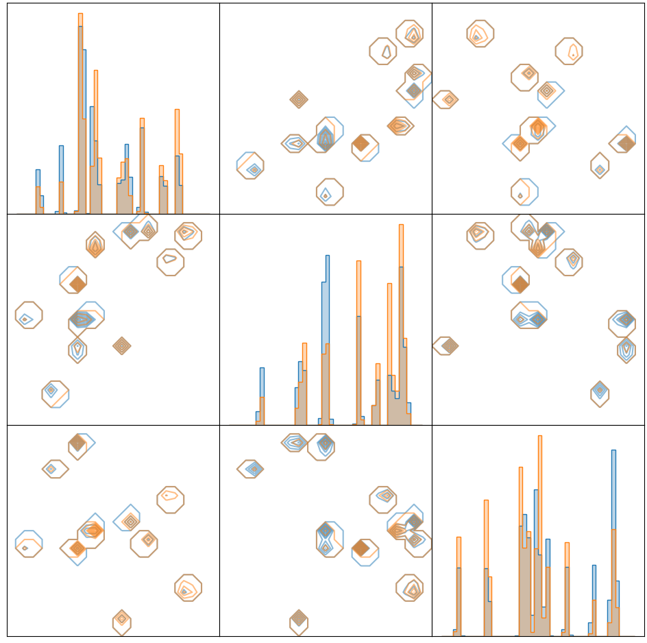
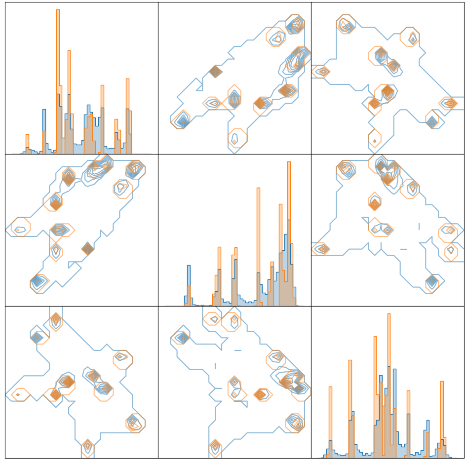
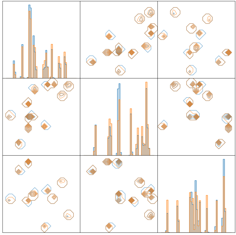
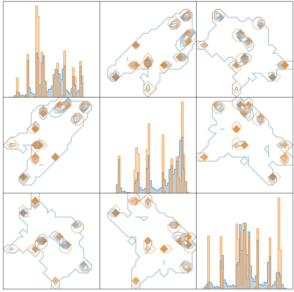
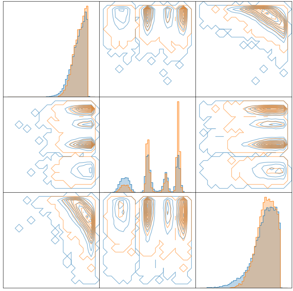
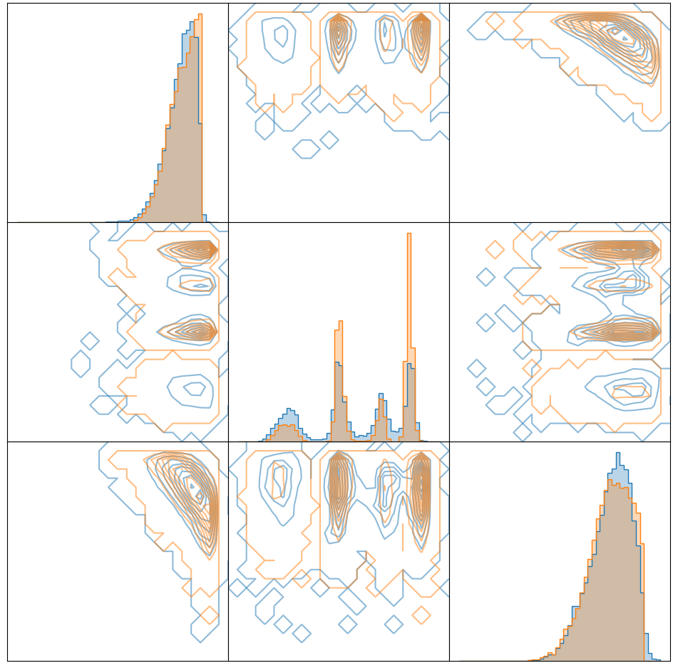
For two exemplar values of $y_{i}$ we plotted histograms of (some marginals of) the samples generated by the ground truth, the conditional SNF and the conditional INN in Figure 1. Here, one can see the topological issues of the conditional INN, which has difficulties to distribute mass to very peaky modes and therefore moves some mass in between them. The MALA layers in the conditional SNF overcome these topological constraints.

Figure 1: Histograms of the first, $50$-th and $100$-th marginal of the ground truth (orange) and the posterior reconstructions using a conditional SNF (left, blue) and a conditional INN (right, blue) for two different samples of $Y$. On the diagonal we plot the one histograms of the one-dimensional marginals, on the off-diagonal we plot the potentials of the two dimensional marginals.

6.2 Example from Scatterometry

Next, we apply the conditional SNFs to a real world inverse problem, where the nonlinear forward operator $F\colon\mathbb{R}^{3}\rightarrow\mathbb{R}^{23}$ describes the diffraction of monochromatic lights on line gratings and is a non-destructive technique to determine the structures of photo masks [23, 24]. The parameters in $x$-space describe the geometry of the line gratings and $Y=F(X)+\eta$ the diffraction pattern. The inverse problem consists now in recovering the geometry given an observation $y$. We assume that the noise $\eta$ is mixed additive and multiplicative Gaussian noise, i.e., $\eta=aF(X)\eta_{1}+b\eta_{2}$, where $\eta_{1},\eta_{2}\sim\mathcal{N}(0,I)$ and $a,b>0$ are some constants. Then, the conditional distribution $P_{Y|X=x}$ is given by $\mathcal{N}\left(F(x),(a^{2}F(x)^{2}+b^{2})\,I\right)$ Here $b$ represents the strength of background noise, while $a$ controls the strength of fluctuations depending on the forward model.

In scatterometry, the forward operator $F$ is known from physics, but its evaluation requires the solution of some partial differential equation [24], which is slow and computationally costly. Therefore, we sample $N=10000$ data points $x_{i}$ uniformly from $[-1,1]^{3}$ and evaluate the exact forward operator $F(x_{i})$, $i=1,...,N$ (which is computationally costly). Then, we approximate $F$ by a feed-forward neural network $\tilde{F}$ with $3$ hidden layers and $256$ neurons in each hidden layer by minimizing the loss function

$$\sum_{i=1}^{N}\|\tilde{F}(x_{i})-F(x_{i})\|^{2}.$$

Throughout this section, we will use this approximation $\tilde{F}$ as our forward operator $F$.

Since we do not have any prior information about the parameters $x$, we choose the prior distribution $P_{X}$ as the uniform distribution on $[-1,1]^{3}$. For the conditional SNF we assumed that $P_{X}$ has a strictly positive density $p_{X}$. To fulfill this assumption, we relax the probability density function of the uniform distribution for $x=(x_{1},x_{2},x_{3})\in\mathbb{R}^{3}$ by

$$p_{X}(x)\coloneqq q(x_{1})q(x_{2})q(x_{3}),\quad q(x)\coloneqq\begin{cases}\frac{\alpha}{2\alpha+2}\exp(-\alpha(-1-x)),&$for $x<-1,\\ \frac{\alpha}{2\alpha+2},&$for $x\in[-1,1],\\ \frac{\alpha}{2\alpha+2}\exp(-\alpha(x-1)),&$for $x>1,\end{cases}$$

where $\alpha\gg 0$ is some constant. Note that for large $\alpha$ and $x_{i}$ outside of $[-1,1]$ the function $q$ becomes small such that $p_{X}$ is small outside of $[-1,1]^{3}$. In our numerical experiments, we choose $\alpha=1000$. Now the density of the posterior distribution $P_{X|Y=y}$ can be evaluated up to a multiplicative constant by Bayes’ theorem as $p_{X|Y=y}(x)\propto p_{Y|X=x}(y)p_{X}(x).$ We can assume for this experiment that $a=0.2$ and $b=0.01$.

Model parameters and training

We train a conditional SNF with $T=8$ layers similarly to the previous example. The layers $\mathcal{K}_{t}$ for $t=1,3,5,7$ are deterministic layers with conditional INNs with $L=1$ layers, where the subnetworks has two hidden layers with $64$ neurons in each hidden layer. We do not use any permutations. The layers $\mathcal{K}_{t}$ for $t=2,4,6,8$ consist of $10$ MCMC steps using the kernel $Q_{t}$ as defined in (27). Here, we set $\sigma=0.4$.

As a comparison, we also implement a conditional INN with $L=4$ layers, where each subnetwork has two hidden layers with $64$ neurons in each hidden layer. Note that this conditional INN has exactly the same number of parameters as the conditional SNF. We train both networks using the Adam optimizer with a batch size of $1600$ and a learning rate of $10^{-3}$ for the loss function (8). For the SNF, we run $40$ epochs, which takes approximately $50$ seconds. Since for the conditional INN it takes longer until the loss saturates, we train the conditional INN for $5000$ epochs, which takes approximately $8$ minutes. Each epoch consists of $8$ steps of the Adam optimizer.

After the training, we approximate the posterior $P_{X|Y=y}$ by the measure $P_{X_{T}|Y=y}$ for the conditional SNF and by the measure $\mathcal{T}(y,\cdot)_{\#}P_{Z}$ for the conditional INN.

Quality measure

Since we do know the ground truth, we use samples generated by the Metropolis-Hastings algorithm as a baseline. To generate a sample from $P_{X|Y=y}$, we run $1000$ steps of the Metropolis Hastings algorithm, i.e., apply $1000$ times the kernel $\mathcal{K}_{\mathrm{MH}}$ from (15), where the density $p$ in (15) is replaced by $p_{X|Y=y}$.

To evaluate the quality of the approximation $P_{X_{T}|Y=y}$ generated by the conditional SNF of $P_{X|Y=y}$, we approximate $\mathrm{KL}(P_{X|Y=y},P_{X_{T}|Y=y})$ as follows: Let $\mathcal{X}=\{x_{i}\mathrel{\mathop{\ordinarycolon}}i=1,...,N\}$, $N=160000$ be samples of $P_{X_{T}|Y=y}$ generated by the conditional SNF and let $\tilde{\mathcal{X}}=\{\tilde{x}_{i}\mathrel{\mathop{\ordinarycolon}}i=1,...,N\}$ be samples from $P_{X|Y=y}$ generated by the Metropolis-Hastings algorithm. We split our domain $[-1,1]^{3}$ into $50^{3}$ cubes $(C_{ijk})_{i,j,k=1}^{50}$ of size $\tfrac{1}{25}$. Then, we approximate $\mathrm{KL}(P_{X|Y=y},P_{X_{T}|Y=y})$ by $\mathrm{KL}(\mu_{\mathrm{MH}},\mu_{\mathrm{SNF}})$, where $\mu_{\mathrm{MH}}$ and $\mu_{\mathrm{SNF}}$ are the discrete measures

$$\mu_{\mathrm{MH}}(i,j,k)\coloneqq\frac{|\tilde{\mathcal{X}}\cap C_{ijk}|}{N},\quad mu_{\mathrm{SNF}}(i,j,k)\coloneqq\frac{|\mathcal{X}\cap C_{ijk}|}{N}.$$

We approximate the the KL divergence $\mathrm{KL}(P_{X|Y=y},\mathcal{T}_{\#}P_{Z})$ analogously.

Results

We approximate the posterior $P_{X|Y=y_{i}}$ by $P_{X_{T}|Y=y_{i}}$ and by $\mathcal{T}(y_{i},\cdot)_{\#}P_{Z}$ for $100$ i.i.d. samples $y_{i}$ of $Y$. Then, the averaged (approximated) Kullback-Leibler divergences $\mathrm{KL}(P_{X|Y=y_{i}},P_{X_{T}|Y=y_{i}})$ and $\mathrm{KL}(P_{X|Y=y_{i}},\mathcal{T}(y_{i},\cdot)_{\#}P_{Z})$ over $100$ observations $y$ is given by $0.58\pm 0.20$ and $0.84\pm 0.29$, respectively.

To check whether $50^{3}$ cubes suffice to approximate the Kullback-Leibler divergence, we also took the same models and evaluated the average KL over 100 observations $y$ with $75^{3}$ cubes and $540000$ samples. Here, we obtained a mean of $0.54$ for the conditional SNF and $0.78$ for the conditional INN, which is close to the results for $50^{3}$ bins.

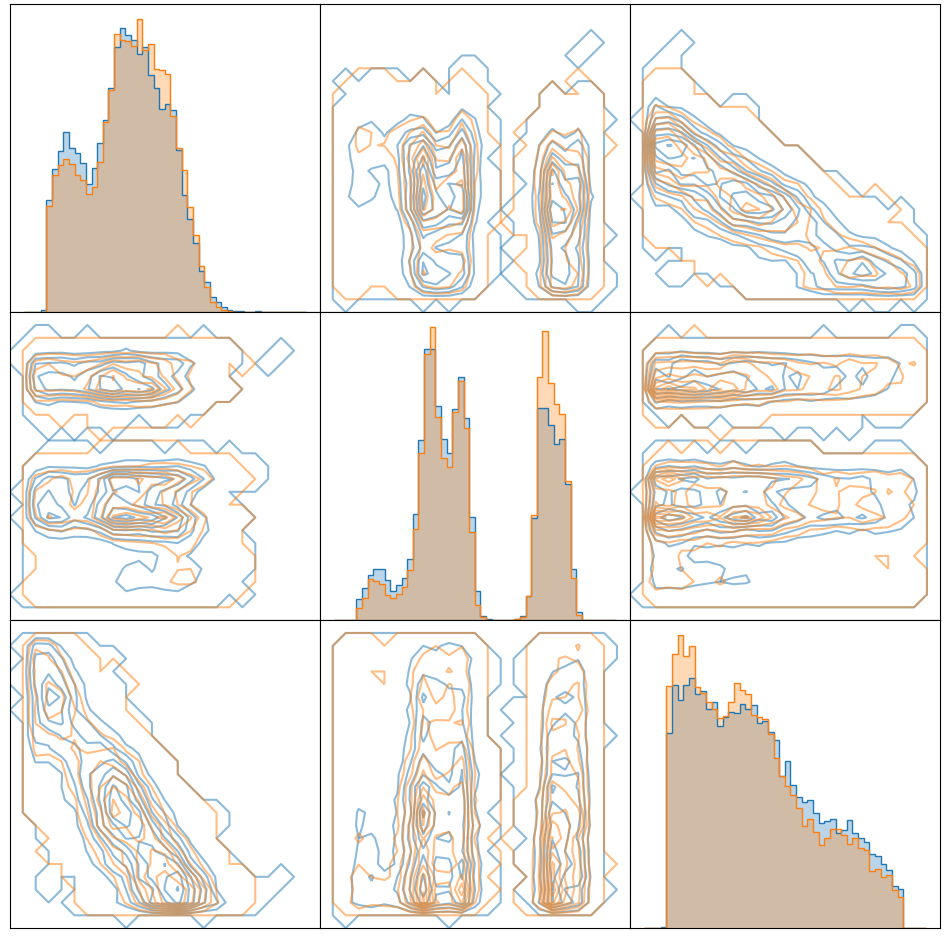
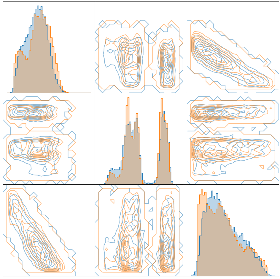
For two exemplar values $y_{i}$, we plotted the histograms of the samples generated by Metropolis Hastings, the conditional SNF and the conditional INN in Figure 2. We observe that the reconstruction using the conditional SNF fits the true posterior generated by the Metropolis-Hastings algorithm better than the reconstruction using the conditional INN, even though the training time of the conditional INN was much longer. In particular, the conditional INN has problems to separate the different modes in the multimodal second component of the posterior.

Figure 2: Histograms of the posterior reconstructions using a conditional SNF (left, blue), a conditional INN (right, blue) and MCMC (orange) for $2$ different samples from $Y$. On the diagonal we plot the one histograms of the one-dimensional marginals, on the off-diagonal we plot the potentials of the two dimensional marginals.

7 Conclusions

We have seen how SNFs can be approached via Markov chains with the advantage that also distributions without densities can be handled in a sound way using general Markov kernels and Radon-Nikodym derivatives. We showed how the concept can be generalized to conditional SNFs for sampling from posterior distributions in inverse problems and gave first numerical examples. As future work, we would like to apply conditional SNFs to inverse problems in imaging. Since the prior distribution $P_{X}$ has to be known, one possibility could be to learn in a first step the prior distribution by an INN as e.g. in [11, 14] or from a patch distribution [25] and to tackle the inverse problem afterwards via a conditional SNF. It would also be interesting to incorporate other layers as variational autoencoders or diffusion flows and to investigate the interplay of both losses of the convex combination [51].

Appendix A Invertible Neural Networks

In this paper, we focus on diffeomorphisms $\mathcal{T}_{t}$ determined by an INN with the architecture proposed in [4]. In the following , we skip the index in the description of the INN $\mathcal{T}_{t}$, but keep in mind that different INNs, i.e. different parameters, are learned for different Markov chain indices $t$. Our INN $\mathcal{T}=\mathcal{T}(\cdot;\theta)$ with parameters $\theta$ is a composition

$$\mathcal{T}=T_{L}\circ P_{L}\circ\dots\circ T_{1}\circ P_{1},$$ (22)

of permutation matrices $P_{\ell}$ and invertible mappings $T_{\ell}$ of the form

$$T_{\ell}(\xi_{1},\xi_{2})=(x_{1},x_{2})\coloneqq\left(\xi_{1}\,\mathrm{e}^{s_{\ell,2}(\xi_{2})}+t_{\ell,2}(\xi_{2}),\,\xi_{2}\,\mathrm{e}^{s_{\ell,1}(x_{1})}+t_{\ell,1}(x_{1})\right)$$

for some splitting $(\xi_{1},\xi_{2})\in\mathbb{R}^{d}$ with $\xi_{i}\in\mathbb{R}^{d_{i}}$, $i=1,2$. Here $s_{\ell,2},t_{\ell,2}\mathrel{\mathop{\ordinarycolon}}\mathbb{R}^{d_{2}}\to\mathbb{R}^{d_{1}}$ and $s_{\ell,1},t_{\ell,1}\mathrel{\mathop{\ordinarycolon}}\mathbb{R}^{d_{1}}\to\mathbb{R}^{d_{2}}$ are ordinary feed-forward neural networks. The parameters $\theta$ of $\mathcal{T}(\cdot;\theta)$ are specified by the parameters of these subnetworks. The inverse of the network layers $T_{l}$ is analytically given by

$$T_{\ell}^{-1}(x_{1},x_{2})=(\xi_{1},\xi_{2})\coloneqq\left(\big{(}x_{1}-t_{\ell,2}(\xi_{2})\big{)}\,\mathrm{e}^{-s_{\ell,2}(\xi_{2})},\,\big{(}x_{2}-t_{\ell,1}(x_{1})\big{)}\,\mathrm{e}^{-s_{\ell,1}(x_{1})}\right)$$

and does not require an inversion of the feed-forward subnetworks. Hence the whole map $\mathcal{T}$ is invertible and allows for a fast evaluation of both forward and inverse map.

In our loss function, we will need the log-determinant of $\mathcal{T}$. Fortunately this can be simply computed by the following considerations: since $T_{\ell}=T_{2,\ell}\circ T_{1,\ell}$ with

$$T_{1,\ell}(\xi_{1},\xi_{2})=(x_{1},\xi_{2}) \coloneqq\left(\xi_{1}\mathrm{e}^{s_{\ell,2}(\xi_{2})}+t_{\ell,2}(\xi_{2}),\xi_{2}\right),$$

$$T_{2,\ell}(x_{1},\xi_{2})=(x_{1},x_{2}) \coloneqq\left(x_{1},\xi_{2}\mathrm{e}^{s_{\ell,1}(x_{1})}+t_{\ell,1}(x_{1})\right),$$

we have

$$\nabla T_{1,\ell}(\xi_{1},\xi_{2}) =\begin{pmatrix}\mathrm{diag}\left(\mathrm{e}^{s_{\ell,2}(\xi_{2})}\right)&\mathrm{diag}\left(\nabla_{\xi_{2}}\left(\xi_{1}\mathrm{e}^{s_{\ell,2}(\xi_{2})}+t_{\ell,2}(\xi_{2})\right)\right)\\ 0&I_{d_{2}}\end{pmatrix}$$

so that $\det\nabla T_{1,\ell}(\xi_{1},\xi_{2})=\prod_{k=1}^{d_{1}}\mathrm{e}^{\left(s_{\ell,2}(\xi_{2})\right)_{k}}$ and similarly for $\nabla T_{2,\ell}$. Applying the chain rule in (22) and noting that the Jacobian of $P_{\ell}$ is just $P_{\ell}$ with $|\det P_{\ell}|=1$, and that $\det(AB)=\det(A)\det(B)$, we conclude

$$\log(|\det\left(\nabla\mathcal{T}(\xi)\right)|)=\sum_{\ell=1}^{L}\left(\operatorname{sum}\left(s_{\ell,2}\left((P_{\ell}\xi^{\ell})_{2}\right)\right)+\operatorname{sum}\left(s_{\ell,1}\left((T_{1,\ell}P_{\ell}\xi^{\ell})_{1}\right)\right)\right),$$

where $\operatorname{sum}$ denotes the sum of the components of the respective vector, $\xi^{1}\coloneqq\xi$ and $\xi^{\ell}=T_{\ell-1}P_{\ell-1}\xi^{\ell-1}$, $\ell=2,\ldots,L$.

Appendix B Proof of Lemma 1

We show the first equation. The second one can be proven analogously using that for a Markov chain $(X_{0},...,X_{T})$ the time-reversal $(X_{T},...,X_{0})$ is again a Markov chain. For $f$ in (9), we consider the measure $\mu\coloneqq f\,P_{(X_{0},...,X_{T})}$ and show that $\mu=P_{(Y_{0},...,Y_{T})}$. For this purpose, let $A_{0}\times\cdots\times A_{T}\subseteq(\mathbb{R}^{d})^{T+1}$ be a measurable rectangle. Then, using that by definition of a regular conditional distribution it holds $P_{(X_{T},X_{0},...,X_{T-1})}=P_{X_{T}}\times P_{(X_{0},...,X_{T-1})|X_{T}}$, we get

$$\mu(A_{0}\times\cdots\times A_{T})=\int\limits_{A_{0}\times\cdots\times A_{T}}\frac{p_{Y_{T}}(x_{T})}{p_{X_{T}}(x_{T})}\prod_{t=1}^{T}f_{t}(x_{t-1},x_{t})\mathrm{d}P_{(X_{0},...,X_{T})}(x_{0},...,x_{T})$$

$$=\int\limits_{A_{T}}\frac{p_{Y_{T}}(x_{T})}{p_{X_{T}}(x_{T})}\int\limits_{A_{0}\times\cdots\times A_{T-1}}\prod_{t=1}^{T}f_{t}(x_{t-1},x_{t})\mathrm{d}P_{(X_{0},...,X_{L-1})|X_{T}=x_{T}}(x_{0},...,x_{T-1})\mathrm{d}P_{X_{T}}(x_{T}).$$

Using that $\frac{p_{Y_{T}}}{p_{X_{T}}}$ is the Radon-Nikodym derivative of $P_{Y_{T}}$ with respect to $P_{X_{T}}$, we obtain

$$\quad\mu(A_{0}\times\cdots\times A_{T})$$

$$=\int\limits_{A_{T}}\int\limits_{A_{0}\times\cdots\times A_{T-1}}\prod_{t=1}^{T}f_{t}(x_{t-1},x_{t})\mathrm{d}P_{(X_{0},...,X_{T-1})|X_{T}=x_{T}}(x_{0},...,x_{T-1})\mathrm{d}P_{Y_{T}}(x_{T}).$$

Thus it suffices to prove for $l=1,...,T$ that

$$I_{l} \coloneqq\int\limits_{A_{0}\times\cdots\times A_{l-1}}\prod_{t=1}^{l}f_{t}(x_{t-1},x_{t})\mathrm{d}P_{(X_{0},...,X_{l-1})|X_{l}=x_{l}}(x_{0},...,x_{l-1})$$

$$=P_{(Y_{0},...,Y_{l-1})|Y_{l}=x_{l}}(A_{0}\times\cdots\times A_{l-1}).$$ (23)

since then

$$\mu(A_{0}\times\cdots\times A_{T}) =\int\limits_{A_{T}}P_{(Y_{0},...,Y_{T-1})|Y_{T}=x_{T}}(A_{0}\times\cdots\times A_{T-1})\mathrm{d}P_{Y_{T}}(x_{T})$$

$$=P_{(Y_{0},...,Y_{T})}(A_{0}\times\cdots\times A_{T})$$

and we are done. We show (23) by induction. Since $f_{1}(\cdot,x_{1})$ is the Radon-Nikodym derivative $\frac{dP_{Y_{0}|Y_{1}=x_{1}}}{dP_{X_{0}|X_{1}=x_{1}}}$, we have for $l=1$ that

$$\int\limits_{A_{0}}f_{1}(x_{0},x_{1})\mathrm{d}P_{X_{0}|X_{1}=x_{1}}(x_{0}) =\int\limits_{A_{0}}1\,\mathrm{d}P_{Y_{0}|Y_{1}=x_{1}}(x_{0})=P_{Y_{0}|Y_{1}=x_{1}}(A_{0}).$$

Now assume that (23) is true for $l-1$. Then it holds

$$I_{l} =\int\limits_{A_{l-1}}\int\limits_{A_{0}\times\cdots\times A_{l-2}}\prod_{t=1}^{l-1}f_{t}(x_{t-1},x_{t})\mathrm{d}P_{(X_{0},...,X_{l-2})|X_{l-1}=x_{l-1},X_{l}=x_{l}}(x_{0},...,x_{l-2})$$

$$\quad\cdot f_{l}(x_{l-1},x_{l})\mathrm{d}P_{X_{l-1}|X_{l}=x_{l}}(x_{l-1}),$$

and by the Markov property of $(X_{T},...,X_{0})$ and the definition of $f_{l}$ further

$$I_{l} =\int\limits_{A_{l-1}}\,I_{l-1}\,\mathrm{d}P_{Y_{l-1}|Y_{l}=x_{l}}(x_{l-1})$$

$$=\int\limits_{A_{l-1}}P_{(Y_{0},...,Y_{l-2})|Y_{l-1}=x_{l-1}}(A_{0}\times\cdots\times A_{l-2})\mathrm{d}P_{Y_{l-1}|Y_{l}=x_{l}}(x_{l-1})$$

$$=\int\limits_{A_{l-1}}P_{(Y_{0},...,Y_{l-2})|Y_{l-1}=x_{l-1},Y_{l}=x_{l}}(A_{0}\times\cdots\times A_{l-2})\mathrm{d}P_{Y_{l-1}|Y_{l}=x_{l}}(x_{l-1})$$

$$=P_{(Y_{0},...,Y_{l-1})|Y_{l}=x_{l}}(A_{0}\times\cdots\times A_{l-1}).$$

Since the measurable rectangles are a $\cap$-stable generator of $\mathcal{B}(\mathbb{R}^{d})$, this proves the claim. $\Box$

Appendix C Deterministic and Stochastic Layers for Conditional SNFs

Deterministic layer: Suppose that $X_{t}\coloneqq\mathcal{T}_{t}(Y,X_{t-1})$ for some measurable mapping $\mathcal{T}_{t}\colon\mathbb{R}^{\tilde{d}}\times\mathbb{R}^{d}\to\mathbb{R}^{d}$ such that $\mathcal{T}_{t}(y,\cdot)$ is a diffeomorphism for any $y\in\mathbb{R}^{\tilde{d}}$. Then we use the Markov kernels given by

$$\mathcal{K}_{t}(y,x,A)\coloneqq\delta_{\mathcal{T}_{t}(y,x)}(A),\quad\mathcal{R}_{t}(y,x,A)\coloneqq\delta_{\mathcal{T}_{t}^{-1}(y;x)}(A),$$

where $\mathcal{T}_{t}^{-1}(y;x)$ denotes the inverse of $\mathcal{T}_{t}(y,\cdot)$ at point $x$.

Such mappings $\mathcal{T}$ can be constructed by using conditional INNs which were introduced in [3, 5] and are closely related to conditional GANs [33]. A conditional INN is a neural network $\mathcal{T}=\mathcal{T}(\cdot,\cdot;\theta)\colon\mathbb{R}^{\tilde{d}}\times\mathbb{R}^{d}\to\mathbb{R}^{d}$ such that $\mathcal{T}(y,\cdot)\colon\mathbb{R}^{d}\to\mathbb{R}^{d}$ is by construction invertible for any $y\in\mathbb{R}^{\tilde{d}}$. In this paper, we use an adaption of the INN architecture (22) to model a conditional INN similarly as in [5]. More precisely, the network $\mathcal{T}(y,\cdot)$ is a composition

$$\mathcal{T}(y,\cdot)=T_{L}(y,\cdot)\circ P_{L}\circ\dots\circ T_{1}(y,\cdot)\circ P_{1},$$ (24)

of permutation matrices $P_{l}$ and mappings $T_{l}\colon\mathbb{R}^{\tilde{d}}\times\mathbb{R}^{d}\to\mathbb{R}^{d}$ of the form

$$T_{l}(y,\xi_{1},\xi_{2})=(x_{1},x_{2})\coloneqq\left(\xi_{1}\,\mathrm{e}^{s_{l,2}(y,\xi_{2})}+t_{l,2}(y,\xi_{2}),\,\xi_{2}\,\mathrm{e}^{s_{l,1}(y,x_{1})}+t_{l,1}(y,x_{1})\right)$$ (25)

for some splitting $(\xi_{1},\xi_{2})\in\mathbb{R}^{d}$ with $\xi_{i}\in\mathbb{R}^{d_{i}}$, $i=1,2$. As before $s_{l,2},t_{l,2}\mathrel{\mathop{\ordinarycolon}}\mathbb{R}^{\tilde{d}}\times\mathbb{R}^{d_{2}}\to\mathbb{R}^{d_{1}}$ and $s_{l,1},t_{l,1}\mathrel{\mathop{\ordinarycolon}}\mathbb{R}^{\tilde{d}}\times\mathbb{R}^{d_{1}}\to\mathbb{R}^{d_{2}}$ are ordinary feed-forward neural networks and the parameters $\theta$ of $\mathcal{T}(\cdot,\cdot;\theta)$ are specified by the parameters of these subnetworks. Note that for any $y\in\mathbb{R}^{\tilde{d}}$ the mapping $T_{l}(y,\cdot)$ is by definition invertible and admits the analytical inverse

$$(T_{l}(y,\cdot))^{-1}(x_{1},x_{2})=(\xi_{1},\xi_{2})\coloneqq\left(\big{(}x_{1}-t_{l,2}(y,\xi_{2})\big{)}\,\mathrm{e}^{-s_{l,2}(y,\xi_{2})},\,\big{(}x_{2}-t_{l,1}(y,x_{1})\big{)}\,\mathrm{e}^{-s_{l,1}(y,x_{1})}\right).$$

We obtain that $\mathcal{T}(y,\cdot)$ is invertible for any $y\in\mathbb{R}^{\tilde{d}}$. Further, both forward and inverse map can be computed very efficiently.

Langevin layer: Let $P_{t}\colon\mathbb{R}^{\tilde{d}}\times\mathcal{B}(\mathbb{R}^{d})\to[0,1]$ be a Markov kernel such that $P_{t}(y,\cdot)$ has the density $p_{t}^{y}\colon\mathbb{R}^{d}\to\mathbb{R}_{>0}$. Further, define $\xi_{t}\sim\mathcal{N}(0,I)$ and $u_{t}^{y}(x)=-\log(p_{t}^{y}(x))$. Then

$$X_{t}\coloneqq X_{t-1}-a_{1}\nabla u^{y}_{t}(X_{t-1})+a_{2}\xi_{t},$$

with $a_{1},a_{2}>0$ has the transition kernel $\mathcal{K}_{t}$ given by

$$\mathcal{K}_{t}(y,x,A)\coloneqq\mathcal{N}(A|x-a_{1}\nabla u_{t}^{y}(x),a_{2}^{2}I).$$

Again, we use $\mathcal{R}_{t}=\mathcal{K}_{t}$ as reverse layer.

MCMC layer: Let $P_{t}\colon\mathbb{R}^{\tilde{d}}\times\mathcal{B}(\mathbb{R}^{d})\to[0,1]$ be a Markov kernel such that $P_{t}(y,\cdot)$ has the density $p_{t}^{y}\colon\mathbb{R}^{d}\to\mathbb{R}_{>0}$. Further, let $Q_{t}\colon\mathbb{R}^{\tilde{d}}\times\mathbb{R}^{d}\times\mathcal{B}(\mathbb{R}^{d})$ be a Markov kernel, such that $Q_{t}(y,x,\cdot)$ admits the strictly positive density $q_{t}^{y}(\cdot|x)$. Define by $X^{\prime}_{t}$ a random variable independent of $(X_{0},...,X_{t-2})$ such that

$$P_{X_{t-1},X^{\prime}_{t}|Y=y}=P_{X_{t}|Y=y}\times Q_{t}(y,\cdot,\cdot)$$

and assume that

$$X_{t}\coloneqq 1_{[U,1]}\big{(}\alpha_{t}^{Y}(X_{t-1},X_{t}^{\prime})\big{)}\,X_{t}^{\prime}+1_{[0,U]}\big{(}\alpha_{t}^{Y}(X_{t-1},X_{t}^{\prime})\big{)}\,X_{t-1}$$

where $\alpha_{t}^{y}(x,w)\coloneqq\left\{\min(1,\tfrac{p^{y}_{t}(w)q_{t}^{y}(x|w)}{p^{y}_{t}(x)q_{t}^{y}(w|x)})\right\}$. Then the transition kernel $\mathcal{K}_{t}$ is given by

$$\mathcal{K}_{t}(y,x,A)\coloneqq\int_{A}q_{t}^{y}(w|x)\alpha_{t}^{y}(x,w)\mathrm{d}w+\delta_{x}(A)\int_{\mathbb{R}^{d}}q_{t}^{y}(w|x)(1-\alpha_{t}^{y}(x,w)))\mathrm{d}w.$$ (26)

Note, that for fixed $y\in\mathbb{R}^{\tilde{d}}$, the kernel $\mathcal{K}_{t}(y,\cdot,\cdot)$ is the Metropolis-Hastings kernel with respect to the density $p^{y}_{t}$ and Markov kernel $Q_{t}(y,\cdot,\cdot)$. Analogously to Remark 4, we consider in our numerical examples the kenels

$$Q_{t}(y,x,\cdot)=\mathcal{N}(x,\sigma^{2}I),\qquad q_{t}^{y}(\cdot|x)=\mathcal{N}(\cdot|x,\sigma^{2}I)$$ (27)

and

$$Q_{t}(y,x,\cdot)=\mathcal{N}(x-a_{1}\nabla u_{t}^{y}(x),a_{2}^{2}I),\qquad q_{t}^{y}(\cdot|x)=\mathcal{N}(\cdot|x-a_{1}\nabla u_{t}^{y}(x),a_{2}^{2}I).$$ (28)

As in the non-conditional case we use $\mathcal{R}_{t}=\mathcal{K}_{t}$ as reverse layer.

References

- [1] A. Andrle, N. Farchmin, P. Hagemann, S. Heidenreich, V. Soltwisch, and G. Steidl. Invertible neural networks versus MCMC for posterior reconstruction in grazing incidence X-ray fluorescence. In A. Elmoataz, J. Fadili, Y. Quéau, J. Rabin, and L. Simon, editors, Scale Space and Variational Methods, volume 12679 of Lecture Notes in Computer Science, pages 528–539. Springer, 2021.
- [2] M. Arbel, A. G. D. G. Matthews, and A. Doucet. Annealed flow transport monte carlo. ArXiv:2102.07501, 2021.
- [3] L. Ardizzone, J. Kruse, C. Lüth, N. Bracher, C. Rother, and U. Köthe. Conditional invertible neural networks for diverse image-to-image translation. In T. S. Z. Akata, A. Geiger, editor, Pattern Recognition: 42nd DAGM German Conference, DAGM GCPR 2020, volume 12544 of Lecture Notes in Computer Science, pages 373–387. Springer, 2021.
- [4] L. Ardizzone, J. Kruse, C. Rother, and U. Köthe. Analyzing inverse problems with invertible neural networks. In International Conference on Learning Representations, 2019.
- [5] L. Ardizzone, C. Lüth, J. Kruse, C. Rother, and U. Köthe. Guided image generation with conditional invertible neural networks. ArXiv:1907.02392, 2019.
- [6] S. Arridge, P. Maass, O. Öktem, and C. B. Schönlieb. Solving inverse problems using data-driven models. Acta Numer., 28:1–174, 2019.
- [7] J. Behrmann, W. Grathwohl, R. T. Chen, D. Duvenaud, and J.-H. Jacobsen. Invertible residual networks. In International Conference on Machine Learning, pages 573–582, 2019.
- [8] J. Behrmann, P. Vicol, K.-C. Wang, R. Grosse, and J.-H. Jacobsen. Understanding and mitigating exploding inverses in invertible neural networks. ArXiv:2006.09347, 2020.
- [9] R. Bergmann, J. H. Fitschen, J. Persch, and G. Steidl. Iterative multiplicative filters for data labeling. Int. J. Comput. Vis., 123(3):123–145, 2017.
- [10] C. Chen, C. Li, L. Chen, W. Wang, Y. Pu, and L. Carin. Continuous-time flows for efficient inference and density estimation. ArXiv:1709.01179, 2017.
- [11] R. T. Q. Chen, J. Behrmann, D. K. Duvenaud, and J.-H. Jacobsen. Residual flows for invertible generative modeling. In Advances in Neural Information Processing Systems, volume 32. Curran Associates, Inc., 2019.
- [12] R. Cornish, A. L. Caterini, G. Deligiannidis, and A. Doucet. Relaxing bijectivity constraints with continuously indexed normalising flows. ArXiv:1909.13833, 2019.
- [13] N. De Cao, I. Titov, and W. Aziz. Block neural autoregressive flow. ArXiv:1904.04676, 2019.
- [14] L. Dinh, J. Sohl-Dickstein, and S. Bengio. Density estimation using real NVP. In International Conference on Learning Representations, 2017.
- [15] C. Durkan, A. Bekasov, I. Murray, and G. Papamakarios. Neural spline flows. Advances in Neural Information Processing Systems, 2019.
- [16] L. Falorsi, P. de Haan, T. R. Davidson, W. De Cao, N., P. M., Forré, and T. S. Cohen. Explorations in homeomorphic variational auto-encoding. ArXiv:1807.04689, 2018.
- [17] L. Falorsi, P. de Haan, T. R. Davidson, and P. Forré. Reparameterizing distributions on Lie groups. ArXiv:1903.02958, 2019.
- [18] R. Flamary, N. Courty, A. Gramfort, M. Z. Alaya, A. Boisbunon, S. Chambon, L. Chapel, A. Corenflos, K. Fatras, N. Fournier, L. Gautheron, N. T. Gayraud, H. Janati, A. Rakotomamonjy, I. Redko, A. Rolet, A. Schutz, V. Seguy, D. J. Sutherland, R. Tavenard, A. Tong, and T. Vayer. POT: Python optimal transport. J. Mach. Learn. Res., 22(78):1–8, 2021.
- [19] M. Girolami and B. Calderhead. Riemann manifold Langevin and Hamiltonian Monte Carlo methods. J. R. Stat. Soc.: Series B (Statistical Methodology), 73(2):123–214, 2011.
- [20] D. Grana, T. Fjeldstad, and H. Omre. Bayesian Gaussian mixture linear inversion for geophysical inverse problems. Math. Geosci., 49(4):493–515, 2017.
- [21] P. L. Hagemann and S. Neumayer. Stabilizing invertible neural networks using mixture models. Inverse Probl., 2021.
- [22] K. He, X. Zhang, S. Ren, and J. Sun. Deep residual learning for image recognition. In Proceedings of the IEEE Conference on Computer Vision and Pattern Recognition, pages 770–778, 2016.
- [23] S. Heidenreich, H. Gross, and M. Bär. Bayesian approach to the statistical inverse problem of scatterometry: Comparison of three surrogate models. Int. J. Uncertain. Quantif., 5(6), 2015.
- [24] S. Heidenreich, H. Gross, and M. Bär. Bayesian approach to determine critical dimensions from scatterometric measurements. Metrologia, 55(6):S201, Dec. 2018.
- [25] J. Hertrich, A. Houdard, and C. Redenbach. Wasserstein patch prior for image superresolution. ArXiv:2109.12880, 2021.
- [26] C.-W. Huang, D. Krueger, A. Lacoste, and A. Courville. Neural autoregressive flows. In International Conference on Machine Learning, pages 2078–2087, 2018.
- [27] P. Jaini, I. Kobyzev, Y. Yu, and M. Brubaker. Tails of lipschitz triangular flows. ArXiv:1907.04481, 2019.
- [28] D. P. Kingma and J. Ba. Adam: A method for stochastic optimization. In International Conference on Learning Representations, 2015.
- [29] D. P. Kingma and P. Dhariwal. Glow: Generative flow with invertible 1x1 convolutions. ArXiv:1807.03039, 2018.
- [30] J. Kruse, G. Detommaso, U. Köthe, and R. Scheichl. HINT: hierarchical invertible neural transport for density estimation and bayesian inference. In AAAI Conference on Artificial Intelligence, pages 8191–8199, 2021.
- [31] J.-F. Le Gall. Brownian motion, martingales, and stochastic calculus, volume 274 of Graduate Texts in Mathematics. Springer, [Cham], 2016.
- [32] T. Minka. Divergence measures and message passing. Technical report, Technical report, Microsoft Research, 2005.
- [33] T. Miyato and M. Koyama. cGANs with projection discriminator. In International Conference on Learning Representations, 2018.
- [34] T. Müller, B. McWilliams, F. Rousselle, M. Gross, and J. Novák. Neural importance sampling. ArXiv:1808.03856, 2018.
- [35] D. Nielsen, P. Jaini, E. Hoogeboom, O. Winther, and M. Welling. SurVAE Flows: surjections to bridge the gap between VAEs and flows. NeurIPS, 2020.
- [36] J. P. Nilmeier, G. E. Crooks, D. D. L. Minh, and J. Chodera. Nonequilibrium candidate Monte Carlo is an efficient tool for equilibrium simulation. Proceedings of the National Academy of Sciences, 108:1009–1018, 2011.
- [37] G. Ongie, A. Jalal, C. A. Metzler, R. G. Baraniuk, A. G. Dimakis, and R. Willett. Deep learning techniques for inverse problems in imaging. IEEE J. Sel. Areas Inf. Theory, 1(1):39–56, 2020.
- [38] G. Papamakarios, T. Pavlakou, , and I. Murray. Masked autoregressive flow for density estimation. Advances in Neural Information Processing Systems, page 2338–2347, 2017.
- [39] D. Rezende and S. Mohamed. Variational inference with normalizing flows. In International Conference on Machine Learning, volume 37 of Proceedings of Machine Learning Research, pages 1530–1538, Lille, France, 2015. PMLR.
- [40] D. J. Rezende and S. Mohamed. Variational inference with normalizing flows. ArXiv:1505.05770, 2015.
- [41] G. O. Roberts and J. S. Rosenthal. General state space Markov chains and MCMC algorithms. Probab. Surv., 1:20 – 71, 2004.
- [42] G. O. Roberts and R. L. Tweedie. Exponential convergence of Langevin distributions and their discrete approximations. Bernoulli, 2(4):341–363, 1996.
- [43] L. Ruthotto and E. Haber. An introduction to deep generative modeling. DMV Mitteilungen, 44(3):1–24, 2021.
- [44] J. Sohl-Dickstein, E. A. Weiss, N. Maheswaranathan, and S. Ganguli. Deep unsupervised learning using nonequilibrium thermodynamics. ArXiv:1503.03585, 2015.
- [45] J. Song, S. Zhao, and S. Ermon. A-NICE-MC: Adversarial training for MCMC. ArXiv:1706.07561, 2018.
- [46] A. Thin, N. Kotelevskii, A. Doucet, A. Durmus, E. Moulines, and M. Panov. Monte Carlo variational auto-encoders. In Proceedings of the 38th International Conference on Machine Learning, volume 139 of Proceedings of Machine Learning Research, pages 10247–10257, 2021.
- [47] D. Tsvetkov, L. Hristov, and R. Angelova-Slavova. On the convergence of the Metropolis-Hastings Markov chains. ArXiv:1302.0654v4, 2020.
- [48] M. Welling and Y. W. Teh. Bayesian learning via stochastic gradient langevin dynamics. In International Conference on Machine Learning, page 681–688, 2011.
- [49] J. Whang, E. M. Lindgren, and A. G. Dimakis. Composing normalizing flows for inverse problems. In International Conference on Machine Learning, 2021.
- [50] H. Wu, J. Köhler, and F. Noé. Stochastic normalizing flows. In Advances in Neural Information Processing Systems, 2020.
- [51] S. Zhang, P. Zhang, and T. Y. Hou. Multiscale invertible generative networks for high-dimensional bayesian inference. ArXiv:2105.05489, 2021.