An experimental study on the multiscale properties of turbulence in bubble-laden flows
Abstract
The properties of bubble-laden turbulent flows at different scales are investigated experimentally, focusing on the flow kinetic energy, energy transfer, and extreme events. The experiments employed particle shadow velocimetry measurements to measure the flow in a column generated by a homogeneous bubble swarm rising in water, for two different bubble diameters ( mm mm) and moderate gas volume fractions (). The two velocity components were measured at high-resolution, and used to construct structure functions up to twelfth order for separations spanning the small to large scales in the flow. Concerning the flow anisotropy, the velocity structure functions are found to differ for separations in the vertical and horizontal directions of the flow, and the cases with smaller bubbles are the most anisotropic, with a dependence on void fraction. The degree of anisotropy is shown to increase as the order of the structure functions is increased, showing that extreme events in the flow are the most anisotropic. Our results show that the average energy transfer with the horizontal velocity component is downscale, just as for the three-dimensional single-phase turbulence. However, the energy transfer associated with the vertical component of the fluid velocity is upscale. The probability density functions of the velocity increments reveal that extreme values become more probable with decreasing Reynolds number, the opposite of the behaviour in single-phase turbulence. We visualize those extreme events and find that regions of intense small scale velocity increments occur near the turbulent/non-turbulent interface at the boundary of the bubble wake.
keywords:
1 Introduction
Particle-laden flows are a central topic in fluid mechanics and omnipresent in nature and technology (Prosperetti & Tryggvason, 2009; Balachandar & Eaton, 2010). While great attention has been given to investigating flows containing suspensions of small inertial, heavy particles (Maxey, 1987; Bec et al., 2006, 2007; Fox, 2014; Ireland et al., 2016a, b; Gustavsson & Mehlig, 2016; Hogendoorn & Poelma, 2018; Dou et al., 2018a, b; Tom & Bragg, 2019; Petersen et al., 2019; Berk & Coletti, 2021), there has been less of a focus on bubbly turbulent flows, partly due to the increased complexity associated with performing experiments or simulations for such flows (Lohse, 2018). Among the various topics relevant to bubbly flows, bubble-induced turbulence (BIT) is an important area for investigation, both for its own fundamental importance and also for understanding bubble motion (Magnaudet & Eames, 2000), deformation (Masuk et al., 2021a; Perrard et al., 2021), coalescence/breakup (Liao & Lucas, 2010; Rivière et al., 2021), clustering mechanisms (Zenit et al., 2001; Maeda et al., 2021), and mixing processes (Alméras et al., 2019) in bubbly flows.
Recently, attention has been given to investigating single-point turbulence statistics in bubble-laden flows. Readers are referred to Risso (2018) and Mathai et al. (2020) for detailed reviews. For flows with low to moderate gas void fraction (), we summarize the following characteristics for homogeneous bubble swarms rising either within a background quiescent or weakly turbulent carrier liquid: (i) the liquid velocity fluctuations are highly anisotropic, with much larger fluctuations in the direction of the mean bubble motion (vertical direction in standard coordinates) (Mudde, 2005; Lu & Tryggvason, 2013; Ma et al., 2020b); (ii) the probability density functions (PDFs) of all fluctuating velocity components are non-Gaussian, and the PDF of the vertical velocity fluctuation is strongly positively skewed, while the other two directions have symmetric PDFs (Riboux et al., 2010; Roghair et al., 2011; Lai & Socolofsky, 2019); (iii) bubbles wakes introduce additional turbulence and enhance turbulence dissipation rates in the vicinity of the bubble surface (Santarelli et al., 2016; Masuk et al., 2021b); (iv) modulation of the liquid mean velocity profile due to interphase momentum transfer, resulting in modifications to the background shear-induced turbulence (Lu & Tryggvason, 2008; Bragg et al., 2021).
Studies that have explored the multiscale properties of bubble-laden turbulence have mainly focused on investigating modifications to the energy spectra of the liquid velocity fluctuations due to the bubbles. Lance & Bataille (1991) were the first to find a power law scaling with a slope of about for the vertical velocity fluctuation in a bubble-laden turbulent channel flows using hot-film anemometry. This scaling that emerges in BIT-dominated flows is in contrast to the classical scaling that appears in many single-phase turbulent flows (Pope, 2000). This scaling was also confirmed by subsequent studies for all the components of the fluctuating fluid velocity, and has been observed both in experiments and direct numerical simulations (DNS) (Riboux et al., 2010; Mendez-Diaz et al., 2013; Pandey et al., 2020; Innocenti et al., 2021) for varying bubble properties.
Beyond the behavior of the energy spectra, knowledge about the multiscale properties of bubble-laden turbulence is quite limited. A pioneering study on this topic is that by Rensen et al. (2005), who performed hot-film anemometry measurements in a bubble-laden water tunnel and found an increase of the second-order structure function for the two-phase case compared with the single-phase case for the same bulk Reynolds number, and that this increase was more pronounced at the small scales than the large scales. Moreover, they considered the probability density functions (PDFs) of the velocity increments and used extended self-similarity (ESS) (Benzi et al., 1993) to show that the flow intermittency is enhanced by the bubbles. Furthermore, they argued that once the bubbles are present in the flow, the dependence of the flow properties on the actual bubble concentration is weak for the range they investigated (). Similar behaviour was also observed later in Biferale et al. (2012) and Ma et al. (2021) when comparing the small-scale properties of bubble-laden and unladen turbulent flows.
To gain more insight into the multiscale energetics of bubble-laden turbulence, Pandey et al. (2020) computed the scale-by-scale average energy budget equation in Fourier space using results from an interface-resolved DNS with several tens of bubbles rising in a initially quiescent flow. They showed that on average there is a downscale energy transfer, just as occurs for the single-phase turbulence in three dimensions (Alexakis & Biferale, 2018). A similar finding was also reported by two more recent DNS studies (Innocenti et al., 2021; Ma et al., 2021). An issue with our previous study (Ma et al., 2021), however, is that the conclusion was drawn based on a one-dimensional dataset, which only allowed us to construct the velocity increments for separations in the spanwise direction of the bubble-laden turbulent channel flow.
Another important point to be quantified is how the bubbles influence the anisotropy of the turbulent flow across the scales. Thanks to significant research efforts, single-phase multiscale anisotropy is understood in considerable detail (Sreenivasan & Antonia, 1997; Biferale & Procaccia, 2005). While phenomenological turbulence theories postulate a return-to-isotropy at small scales (Kolmogorov, 1941; Frisch, 1995), experimental and numerical data have showed persistent small-scale anisotropy (Shen & Warhaft, 2000; Ouellette et al., 2006; Pumir et al., 2016), especially when considering high-order structure functions (Carter & Coletti, 2017; Kurien & Sreenivasan, 2000). In contrast to single-phase turbulence, where anisotropy is usually injected into the flow at the large scales (Chang et al., 2012), bubbles inject anisotropy into the flow at the scale of their diameter/wake, and this often corresponds to the small-scales of the turbulence. As a result of this, bubble-laden turbulent flows can exhibit much stronger anisotropy at the small-scales of the flow compared to their single-phase counterparts with the same bulk Reynolds number (Ma et al., 2021). This behavior was quantified in our recent study by developing a new method based on the barycentric map approach (Banerjee et al., 2007), and the results also revealed that the bubble Reynolds number is the key factor responsible for governing the flow anisotropy, whereas the void fraction does not seem to play an important role, at least for the void fractions considered.
To advance the understanding of the multiscale properties of bubble-laden turbulence, in this paper we present an experimental study based on measurements of millimetre-sized air bubbles with (approximately) fixed shape/size rising in a vertical column of water, using high-resolution particle shadow velocimetry (PSV). The water is deliberately contaminated to allow for the no-slip condition to be satisfied on the bubble surface (Elghobashi, 2019), similar to what is usually assumed in DNS studies. The bubbles are injected uniformly at a low to moderate gas void fractions to minimize the large scale velocity fluctuations in the flow (Harteveld et al., 2003), and we focus on a region of the flow sufficiently far away from the walls of the column where the one-point statistics from both phases are approximately homogeneous across the measurement window. Unlike our previous study that used a one-dimensional DNS dataset (Ma et al., 2021), PSV measures two-dimensional, two component (2D-2C) velocity fields, providing access to both longitudinal and transverse structure function associated with separations along two directions. Moreover, we record a large number of uncorrelated velocity fields, so that structure functions up to twelfth-order can be computed. One of the ways the present work advances that in Ma et al. (2021) is that the resolution of the DNS used in Ma et al. (2021) was insufficient to resolve extreme fluctuations in the flow, and therefore only structure functions up to order four were considered. Here, since experimental data is used there is no question regarding whether the physics of the flow is properly captured in the measured quantities.
The rest of this paper is organized as follows. In § 2, we introduce the experimental set-up and the measurement techniques. We then first present the single-point statistics for both phases in § 3. The multipoint results are divided into three parts, namely, anisotropy in § 4, energy transfer in § 5, and intermittency in § 6.
2 Experimental setup and measurement techniques
2.1 Experimental facility
The experimental data required for the present study has only recently become available thanks to the advance of the PSV measurement technique for two-phase flows (Hessenkemper & Ziegenhein, 2018). We used this method in our experiments, which were conducted in Helmholtz-Zentrum Dresden – Rossendorf, Germany. The experimental setup consists of a rectangular column (depth and width ) made of acrylic glass which is filled with tap water to a height of (figure 1). The temperature in the lab was kept constant at and the density and kinematic viscosity of the water are assumed to be constant with values and , respectively.
To suppress bubble deformation, 1-Pentanol is added to the flow. As demonstrated by Tagawa et al. (2014), 1-Pentanol at such a high concentration leads to a rapid full contamination of the bubbles. The thereby induced immobilization of the otherwise mobile bubble surface results in a nearly no-slip condition at the gas-liquid interphase (Takagi & Matsumoto, 2011; Manikantan & Squires, 2020). A reduction of the bubble rising velocity can also be clearly observed in the experiment by adding this amount of 1-Pentanol, which is explained by the Marangoni effect (Takagi & Matsumoto, 2011). Another feature of 1-Pentanol is that the adsorbed surfactant inhibits bubble coalescence and break-up, so that in each experiment the bubbles are mono-disperse with a fixed bubble size.
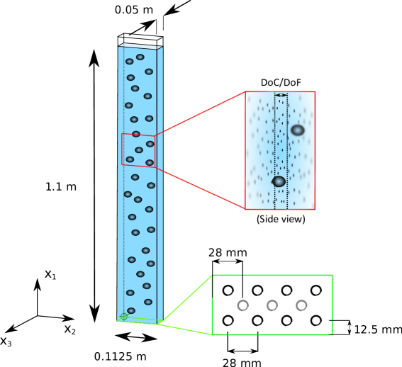
Air bubbles are injected through several spargers that are inserted into holes that have been drilled into the bottom of the column (see bottom right of figure 1 for the sparger configuration). All the spargers are removable, hence, both the gas fraction and the bubble size can be varied by removing or replacing different spargers. In the present study, either all spargers or the outer spargers are used to ensure a homogenous bubble distribution at the measurement height. Here, we use two different spargers with the inner diameter and , corresponding to a constant gas flow rate of and per sparger, respectively (our preliminary tests show that these flow rates lead to a stable production of bubbles of constant size). In summary, we consider two different bubble sizes, and for each bubble size we consider two gas void fractions. These four mono-dispersed cases are labelled as SmLess, SmMore, LaLess, and LaMore in table 1 (Sm/La for smaller/larger bubbles and More/Less for higher/lower gas void fraction), including some basic characteristic dimensionless numbers for the bubbles.
2.2 Measurement techniques
2.2.1 Liquid velocity measurement
Although it is possible to use conventional particle imagine velocimetry (PIV) with a laser-sheet to measure the liquid velocity in bubbly flows, such a side-wise high intensity illumination can result in an inhomogeneous illumination due to unwanted lateral shadows of the bubbles as well as strong light scattering and reflection at the gas-liquid interfaces (Bröder & Sommerfeld, 2007; Tropea, 2011; Ziegenhein & Lucas, 2016). To circumvent these problems, the very recently developed PSV method for dispersed two-phase flows (Hessenkemper & Ziegenhein, 2018) is performed here. The feature of such a measurement is to use a volumetric direct in-line illumination with e.g. LED-backlights for the region of interest, whereby scattering effects are strongly reduced and no lateral bubble shadows occur. By using a shallow depth of field (DoF), sharp tracer particle shadows positioned inside the DoF region can be identified and the particle displacement is evaluated in a PIV-like manner. Hence sometimes this method is also called ‘PIV with LED’ or ‘particle shadow image velocimetry’ (Estevadeordal & Goss, 2005). The top right of figure 1 shows a representation of such a shallow DoF based on the side view of the column. This kind of thin DoF is also frequently used in laser-based PIV measurements, since a laser-sheet thickness below is hard to achieve, while the DoF can be adjusted to even smaller depth expansions (Wereley & Meinhart, 2010). With the present setup, the effective DoF (i.e., depth of correlation (DoC) in the terminology of measurement) is calculated using eq.(2) in Bourdon et al. (2006) as , which is approximately one seventh of the smaller bubble diameter (table 1).
The liquid velocity measurements are performed along the - symmetry plane at the centre of the depth (). In the following, we refer to and as the vertical and horizontal direction, respectively. The measurement height is based on the centre of the field of view (FOV) (figure 1) to ensure that bubbles entering the measurement region have already lost any memory of the way they were injected. The flow is seeded with hollow glass spheres (HGS) – Dantec, and illuminated by a LED-lamp, which consists of small LED arrays arranged in a circular area of diameter and located directly facing the high-speed camera in the -direction. Since the HGS particles are hydrophilic, almost no flotation due to the added surfactant occurs. To fully capture the small-scale fluctuations of the flow, the Stokes number of the seeding particle, defined as must be much smaller than unity, where is the particle response time and is the characteristic time scale of the flow. In the current experiments the highest is for based on the estimated Kolmogorov time scale (table 2), whose estimate is explained in § 3. Image pairs for the velocity determination are acquired with a MotionPro Y3 high-speed CMOS camera, with a frame rate of fps for the smaller bubble cases and 1,100 fps for the larger bubble cases.
Before the velocity interrogation is performed, the comparably large bubble shadows are masked and only interrogation areas outside the mask are considered. Velocity fields are processed using a multipass-refinement procedure, with a final interrogation window size of pixels and overlap. Measurements are obtained by mounting a macro lens (Samyang) with a focal length of and an f-stop of . This provides a FOV of , with a pixel size of m. Since this pixel size is even slightly larger than the seeding particle size, the so-called particle sharpening step (Hessenkemper & Ziegenhein, 2018) is used, which artificially increases the particle size due to a swelling to the neighbouring pixels. Hence, an effective particle size of about - pixels is achieved. In the resulting liquid velocity fields, the spatial resolution (PSV grid) is approximately (, see table 1 for different cases). For more details on the PSV method used in the present measurements, including the whole PIV-like post-processing steps, we refer the readers to Hessenkemper & Ziegenhein (2018).
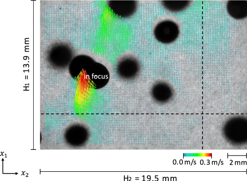
In figure 2 a typical instantaneous FOV with the bubbles and the resulting liquid velocity vector field are shown for the case SmMore. In this snapshot, while there is only one in-focus bubble (identified by the sharp interface), with strong wake entrainment identified in the velocity vector field, the other bubbles are blurred, i.e. out-of-focus. Tracer particles at these locations cannot be detected, so that no liquid velocity fields are available there.
To obtain converged high-order statistics, for each case considered velocity fields were recorded with an image pair acquisition rate of . With interrogation windows in each velocity field, this yields in total data points for each case.
2.2.2 Bubble statistics measurement
| Parameter | SmLess | SmMore | LaLess | LaMore |
|---|---|---|---|---|
| 0.26% | 0.54% | 0.93% | 1.31% | |
| 2.7 | 2.7 | 3.8 | 3.9 | |
| 1.12 | 1.12 | 1.3 | 1.3 | |
| 437 | 437 | 730 | 759 | |
| 1.05 | 1.05 | 2.08 | 2.19 | |
| 524.4 | 522 | 828.5 | 809.5 | |
| 0.925 | 0.931 | 1.027 | 1.158 | |
| 11.6 | 11.6 | 16.4 | 16.8 |
The bubble statistics and properties are evaluated with a separate set of measurements. For these measurements, the flow configurations are kept exactly the same with the exception that no tracer particles are added to the flow and that a larger FOV of (width height) than with PSV for the liquid phase is investigated to obtain sufficient bubble statistics. Here, we have evaluated such image pairs for each case considered.
A machine learning procedure is used to detect and intersect overlapping bubbles in the images (Hessenkemper et al., 2021). The underlying neural network uses a U-Net architecture (Ronneberger et al., 2015) and is trained to find the intersection boundary of a bubble in front of another bubble. Using these intersections, the bubbles are split and an ellipse is fitted to the contour of each bubble. The ellipse parameters are then used to calculate the volume of an axisymmetric spheroid. Since the gas fraction is comparably small, the number of overlapping bubbles is also small and up to now unevaluated errors connected to this are estimated to about . Due to the contamination of the bubbles, deviations from an ellipse due to irregular (wobbling) bubble surfaces are only minor. Example images for the two different bubble sizes with fitted ellipses are given in figure 3 for the cases SmMore and LaLess, respectively. The bubble size is then calculated using the volume-equivalent bubble diameter of a spheroid as , where and are the lengths of the major and minor axes of the fitted ellipse, respectively. For the smaller bubbles, the shape is close to a sphere with a small aspect ratio and we obtain corresponding to an Eötvös number, in our system. In contrast with the larger bubbles, we have , , and . Here, is the density difference between the carrier phase and the dispersed phase and is the surface tensor coefficient. The range of the bubble Reynolds number, , in our experiments are based on and the bubble to liquid relative velocity. Note that although no net liquid flow through a cross-section (- plane) is present (i.e. the bulk velocity of the liquid is zero), for bubble columns, the flow exhibits a large-scale circulation in a time-averaged sense with upward flow in the centre and downward flow close to the walls (Mudde, 2005). This results in a non-negligible upward flow in the measurement area of the present PSV (shown later in § 3), so that the relative velocity in the FOV is in general not equal to the bubble terminal rising velocity. Table 1 lists all the relevant parameters for the bubble properties.
(a)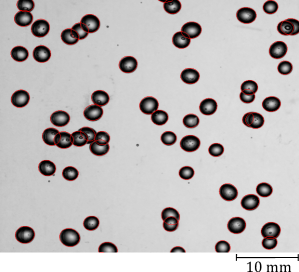
(b)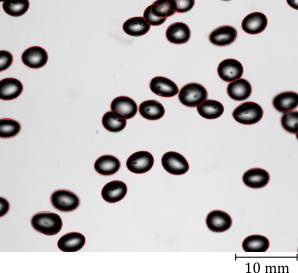
A shallow DoF is used for the measurements conducted to obtain bubble statistics, but it is an order of magnitude larger than that for the liquid velocity measurements due to the different optical system for these two sets of experiments. To measure the bubbles in the -centre region where the liquid velocity measurements were also taken, the average grey value derivative along the bubble contour is calculated. A threshold for this average grey value derivative is used so that only bubbles in the -centre region are considered, and the depth of this -centre region is about . Hence, the evaluated depth for the gas phase is an order of magnitude larger than for the liquid velocity, which is however necessary due to the size of the bubbles. The number of bubbles that fall into this region () is between and summed up over the considered image pairs depending on the case being considered, and this corresponds to an average void fraction range of to (table 1). The bubble velocity was determined by calculating the distance translated by individual bubble centroids, using a standard particle tracking velocimetry algorithm that matches the closest neighbouring bubble in a small search window in the presumed direction of bubble motion (Bröder & Sommerfeld, 2007).
3 Basic flow characterisation
(a)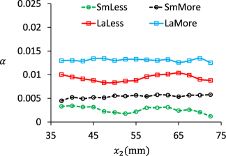
(b)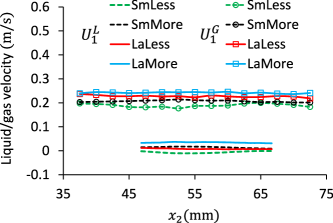
(c)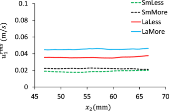
(d)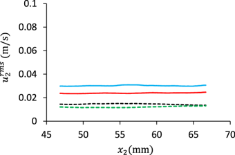
Before exploring the properties of the flow at different scales, we begin with some basic characteristics of the flow as quantified by single-point statistics of both phases. The instantaneous velocity is decomposed into a ensemble-averaged part and a fluctuating part , with associated components .
For all the cases investigated, it is observed that the local void fraction (figure 4a), the vertical gas/liquid mean velocity (figure 4b), and the liquid fluctuating velocity profiles (figure 4c,d) in the observation region (FOV of either liquid or gas) of the column are constant to a very good approximation, impllying statistical homogeneity of the flow in the observation region. As mentioned earlier, for most cases there is a slight upwards mean flow for the liquid phase in the FOV.
According to figure 4, the r.m.s. value of the vertical velocity fluctuation is significantly larger than the horizontal component for the each case, indicating the large scale anisotropy in the flow due to the preferential direction of the bubble motion. The ratio of the vertical to horizontal velocity fluctuation is in the range to for the four cases investigated, which is close to the previous studies of Riboux et al. (2010) and Ma et al. (2021) for bubbles with sizes in the range to . For both components, we find the velocity fluctuations increase with increasing – from SmLess to LaMore.
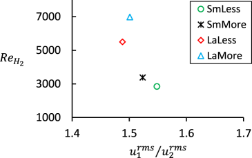
Following Ma et al. (2021), we define a Reynolds number which indicates the range of scales in the turbulent bubbly flows. Here, , and is the weighted turbulent kinetic energy (TKE), , assuming axisymmetry of the flow in the FOV about the vertical direction, and averaged over the FOV of the liquid phase. Note that for our experiments the bulk Reynolds number is zero, since there is no averaged net liquid flow when averaged over the entire flow cross section. Moreover, we are interested in the properties of the fluctuating velocity field, and hence it is more appropriate to consider a Reynolds number based on .
In figure 5 we plot versus large-scale anisotropy ratio (averaged over the FOV of liquid). The figure shows that increases in the order of SmLess, SmMore, LaLess to LaMore, which corresponds to larger bubbles and higher void fraction. Since the Reynolds number of the flow is usually understood to be related to the range of excited scales of motion in the system, this result implies that in the aforementioned sequence the range of excited scales also increases in the flow, hence, the flow becomes increasingly multiscale. Furthermore, we find that for large scales whose velocities are characterized by and , the smaller bubbles produce more anisotropy in the flow than the larger bubbles, as indicated by a larger ratio of for the cases SmLess and SmMore. This is in very close agreement with our previous study based on DNS data of bubble-laden turbulent channel flow driven by a vertical pressure gradient (Ma et al., 2021).
To quantify the PSV resolution with respect to the Kolmogorov scale , we estimate the mean dissipation based on an algebraic relation derived by Ma et al. (2020a) for BIT dominated flows
| (1) |
where the interfacial term for the TKE transport equation is adopted from Ma et al. (2017)
| (2) |
Here, is the mean slip velocity between the bubble and the liquid, and is the drag force on the bubbles averaged over the FOV of the liquid. We can then compute the Kolmogorov length scale , as well the time scale . Both parameters and the ratio of (ranges between and ) are given in table 2 for all the cases. The current PSV spatial resolution and the size of the liquid FOV are comparable to the recent experimental study of Carter & Coletti (2017) on single-phase turbulence using standard PIV (see their small FOV/high resolution measurement).
| Parameter | SmLess | SmMore | LaLess | LaMore |
|---|---|---|---|---|
| 2849 | 3383 | 5502 | 6982 | |
| 0.0147 | 0.0174 | 0.0283 | 0.0359 | |
| 1.54 | 1.52 | 1.49 | 1.50 | |
| 0.0049 | 0.0103 | 0.0199 | 0.0268 | |
| 0.13 | 0.11 | 0.088 | 0.082 | |
| 16.4 | 11.4 | 7.7 | 6.7 | |
| 1.8 | 2.2 | 2.6 | 2.8 |
(a)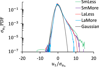
(b)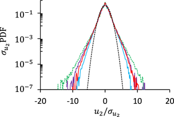
In figure 6 we plot the PDFs of the liquid velocity fluctuations for both directions, normalized by their standard deviations. Due to the large quantity of velocity fields recorded from the experiment, the PDFs are well converged with tails extending to extreme values, and values of the PDF spanning six orders of magnitude, which is much greater than previous experiments for bubbly flows (Riboux et al., 2010; Alméras et al., 2017; Lai & Socolofsky, 2019). Both the vertical and horizontal velocity PDFs are in good quantitative agreement with the previous experimental studies just mentioned. While PDFs of the horizontal velocity fluctuations are symmetric and non-Gaussian, for the vertical component, the PDFs are strongly positively skewed for all the cases. This positive asymmetry originates from the wake entrainment as visualized in figure 2 for the region directly behind the in-focus bubble, which leads to a larger probability of upward fluctuations. The asymmetry of the PDFs is highest for the case SmLess with the the lowest gas void fraction and gradually reduces at larger . In our four cases, increases with increasing , and a similar trend was also reported in figure 5(a) of Prakash et al. (2016). Furthermore, for the PDF of the horizontal velocity component, SmLess is the furthest from Gaussian, associated with stronger large-scale intermittency than the other cases. In many aspects, those results are very different from those of homogeneous isotropic turbulence (HIT) for single-phase flows, for which the PDFs of the velocity fluctuations are almost Gaussian (Gotoh et al., 2002).
4 Turbulence anisotropy quantified using structure functions
While Kolmogorov’s theory assumes local isotropy at the small-scales of turbulent flows (Kolmogorov, 1941, K41 for brevity), many experimental and DNS results reveal persistent anisotropy because the process of a return to isotropy at progressively smaller scales can be very slow (Pumir & Shraiman, 1995; Shen & Warhaft, 2000; Ouellette et al., 2006; Carter & Coletti, 2017). The most systematic approach for characterizing anisotropy at different scales is based on the use of irreducible representations of the SO(3) group (Arad et al., 1999; Biferale & Procaccia, 2005). However, this method requires information on from the complete 3D flow fields, which is often not available. Due to this practical difficulty, many studies on turbulence anisotropy are based on the velocity structure function tensor, and then characterizing anisotropy based on how this quantity varies in different flow directions. The -th order structure function is defined as
| (3) |
where is the fluid velocity increment, and denotes an ensemble average. The calculation of liquid velocity increments in a bubbly flow is, however, delicate, since the liquid velocity is not defined at points occupied by a bubble. To overcome this non-continuous velocity signal challenge, we use the method proposed in (Ma et al., 2017) – store only liquid velocity data along the horizontal/vertical PSV grid lines whenever the entire line was free from bubbles in the considered FOV (see the two dashed lines in figure 2 as example). Based on the velocity fields that were recorded for each case, we were able to extract data along to such vertical/horizontal lines, depending on the case.
4.1 Second-order structure function
We first consider the second-order structure function, whose components are
| (4) |
Hereafter, we suppress the space and time arguments since we are considering a flow which is statistically homogeneous and stationary flows over the FOV. The PSV technique provides access to data associated with separations along two directions, namely, the vertical separation () and the horizontal separation (). Hence, we are able to compute the four contributions
| (5) |
| (6) |
| (7) |
| (8) |
based on the Cartesian coordinate system depicted in figure 1. For an incompressible and isotropic flow, the following relation holds for the transverse structure function
| (9) |
where no summation over is implied.
Figure 7 shows all the measured components of the second-order structure function, as well as obtained from (9) for the representative case SmLess in figure 7(a,d). The results show that the values of the structure functions increase in the order SmLess, SmMore, LaLess, and LaMore, which corresponds to increasing , gas void fraction, and/or bubble Reynolds number. This relationship holds for all of the components computed and across all scales. A similar trend was also reported for all three diagonal components of the second-order structure function based on separations in the spanwise direction of a bubble-laden turbulent channel flow in our recent study (Ma et al., 2021). At the large-scales of a homogeneous flow both and approach unity. Our data for these normalized quantities show that along the separation the quantities converge to unity when . However, while approaches unity, for all the cases. This implies that the FOV is not large enough in the vertical direction to resolve the integral lengthscale of the flow in this direction, while it is for the horizontal direction. However, this may be simply due to the fact that for the FOV.
(a)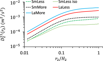
(b)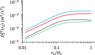
(c)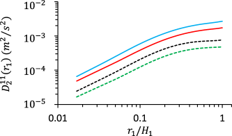
(d)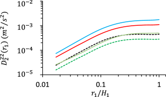
For the SmLess case, departures from are larger at the large scales, reflecting the large scale anisotropy characterized by e.g. in table 2. At for smallest values of , . However, for separations along the vertical direction there are strong departures from at all scales (figure 7d). We obtained similar results (not shown) for the other three cases. Interestingly, such behavior was also observed in Carter & Coletti (2017) for single-phase turbulence generated by jet-stirring (with zero-mean-flow) at a similar range of .
(a)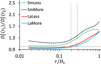
(b)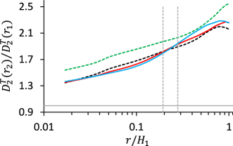
For the second-order structure functions, one of other ways to quantify anisotropy is by the ratios of components such as and , which would be equal to unity for an isotropic flow. The results in figure 8 show that both ratios monotonically decrease for decreasing separation. While the ratio of the longitudinal structure functions is very close to unity at small scales, the ratio of transverse structure functions departs more strongly from unity. By comparing the different cases, the results indicate that the smaller bubbles generate stronger anisotropy in the flow than the larger bubbles across the scales, which is in agreement with the DNS results in Ma et al. (2021) and also the results of large-scale anisotropy in § 3.
In general, the differing behaviour of the second-order structure function in the longitudinal and transverse directions shows that both need to be considered in order to fully consider the turbulence anisotropy across scales. This conclusion based on our bubble-laden flow is in agreement with that of Carter & Coletti (2017) for single-phase turbulence.
4.2 High-order structure function
(a)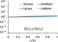
(b)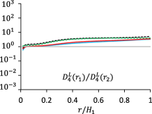
(c)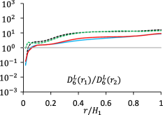
(d)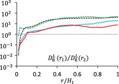
(e)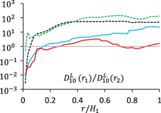
(f)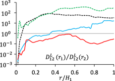
(a)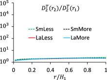
(b)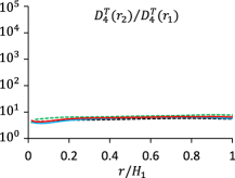
(c)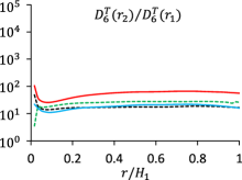
(d)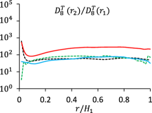
(e)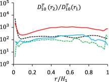
(f)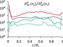
Next, we consider measures of the anisotropy based on even-order structure functions up to order twelve by considering the ratios and which would be equal to unity for an isotropic flow. Using higher order structure functions allows for a characterization of how anisotropic the large fluctuations in the system are. The results in figures 9 and 10 show that the data is statistically well converged up to order 8. For order 10 and 12, although there is considerable noise, the general trend of the results seems clear. The results show that the ratios and deviate increasingly strongly from unity as is increased, with the results for reaching values very far from unity across most of the flow scales. This shows that extreme fluctuations in the flow are more anisotropic than the “typical” fluctuations characterized by the results. Similar behavior has also been observed for single-phase turbulence, showing that higher-order moments are the most anisotropic (Kurien & Sreenivasan, 2000; Warhaft & Shen, 2002). For the longitudinal directions, the results show that just as for the results, the cases with smaller bubbles exhibit greater anisotropy that those with larger bubbles. However, for the transverse direction the LaLess case is by far the most anisotropic. We are not aware of a good explanation for this differing dependence of the longitudinal and transverse anisotropy on the properties of the bubbles.
5 Energy transfer
We now turn to consider the mean energy transfer in the flow, by analysing the third-order structure function as well as the related inter-scale energy transfer term (Hill, 2001; Alexakis & Biferale, 2018)
| (10) |
that appears in the Karman-Howarth type equation governing , where . Note that the divergence term in (10) has been written using the variable to emphasize that this term involves the divergence evaluated at .
The sign of indicates the direction of the non-liner energy transfer between the scales of the flow, and in three-dimensional single-phase turbulence, we have in the inertial and dissipation ranges, corresponding to a downscale transfer of energy from large to small scales on average. With our 2D PSV data we are not able to construct the full quantity , however, we are able to consider some of the contributions .
(a)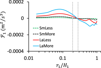
(b)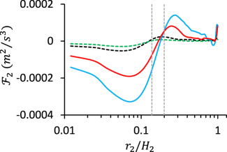
In figure 11 we plot the components and . The peaks in the magnitudes of both and increase in the sequence SmLess, SmMore, LaLess, and LaMore, which corresponds to higher , , and/or . This is in part simply due to the fact that the kinetic energy in the flow increases in this sequence also, and with more kinetic energy at the large scales, there is more available to be passed downscale. Concerning , the results show that at scales , corresponding to energy moving downscale, while at scales , , corresponding to energy moving upscale. In contrast to , the contribution shows an opposite trend, with for at smaller scales indicating a downscale energy transfer. The magnitude of is, however, in general much larger than , implying a higher energy transfer rate in the horizontal direction of the flow. At the low Reynolds number of the flow, there is no inertial range over which either or are constant, indicating that the nonlinear energy transfer is not in the form of a constant flux cascade.
Our previous study (Ma et al., 2021) explored bubble-laden turbulent channel flows and also observed that there is a downscale energy transfer for (where in that paper the 3 direction corresponded to the spanwise direction of the channel flow). However, in that study we could not compute either (streamwise) or (wall-normal) due to the one-dimensional data set being used. Although the type of flow presently under consideration is considerably different from a pressure driven bubble-laden turbulent channel flow, the results nevertheless indicate that the nonlinear energy transfer behaviour may be very different in the different directions of the flow.
These results therefore show that the direction of the energy flux can differ from one direction to another, with revealing an upscale energy transfer at smaller scales, while reveals the opposite. Therefore, although the total energy transfer may be downscale in bubble-turbulent flows (Pandey et al., 2020), some directions of the flow can exhibit an upscale transfer.
(a)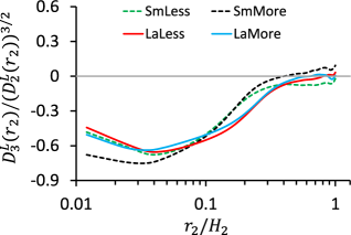
(b)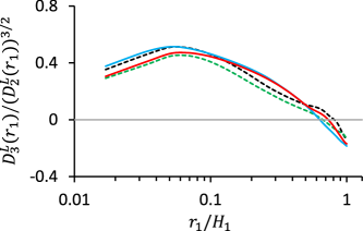
The energy transfer term depends on the third-order structure function, and its behavior may be further understood by considering the associated skewness of the velocity increments. Figure 12 shows (the skewness of the longitudinal velocity increment) for the two separations and . The results show that when is plotted in this normalized form, the results for all of the cases almost collapse, and is not far from the value that occurs for single-phase isotropic turbulence (Davidson, 2015) for . The negative longitudinal skewness along the separation perpendicular to the bubble motion direction was also found in Ma et al. (2021) for some of the bubble-laden cases considered, however for other cases this skewness was actually positive. This is very different from our results where all the cases considered have very similar negative values of the skewness. It is not clear as to whether this is due to the different kinds of flows being studied here and in Ma et al. (2021), or perhaps also because of differences in the parameter space of the bubbles being explored. For vertical separations , also almost collapses for all the cases but is positive at the small scales with a similar magnitude to the results for . This again indicates strong anisotropy for the odd-order structure functions, just as for the even-order structure functions discussed in § 4.
Similar plots are obtained for the transverse structure functions and . The corresponding skewness values were found to be close to zero in both separations directions for all the cases (not shown here).
6 Extreme fluctuations in the flow
Having considered the flow anisotropy and nonlinear energy transfer, we now turn to consider the extreme fluctuations in the flow. Single-phase turbulence at high Reynolds number exhibits fluctuations in space and time of its small-scale quantities that are orders of magnitude larger than the average values, a phenomenon referred to as small-scale intermittency (Frisch, 1995; Sreenivasan & Antonia, 1997). Such extreme fluctuations are critical for many processes in both nature and engineering (Sapsis, 2021), and their investigation continues to be an area of active research (Yeung et al., 2015; Buaria et al., 2019). However, very few studies have explored the topic of intermittency in bubble-laden turbulent flows (see the related works introduced in § 1). In what follows, we focus on extreme fluctuations of the velocity increments in the bubble-laden flow we are considering.
6.1 Probability density functions
(a)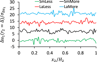
(b)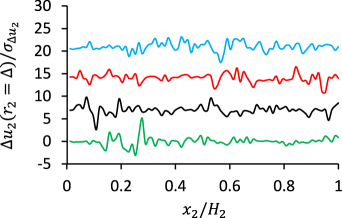
Figure 13 shows the instantaneous velocity increment , normalized by their standard deviation along a line (without bubbles) in the direction of within the FOV. The plots reveal intermittent fluctuations of , with relatively small regions where takes on large values, between which there are relatively small fluctuations of . We will return later to consider how these intermittent large fluctuations of are associated with the bubble wakes in the flow.
(a)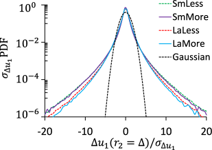
(b)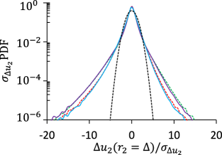
(c)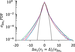
(d)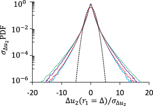
To statistically quantify the extreme events in the flow, the PDFs of the velocity increments can be considered, and these are shown in figure 14, normalized by the standard deviation, for separations equal to one PSV grid . All of the results in figure 14 show that the velocity increments have strongly non-Gaussian PDFs, consistent with the observations based on figure 13. While the PDFs of the transverse velocity increments in plots (a,d) are almost symmetric, the PDFs of the longitudinal velocity increment are negatively skewed for horizontal separations , plot (b), and positively skewed for vertical separations , plot (c), consistent with the skewness results in figure 12. The results also show that the PDFs become increasingly non-Gaussian in the order of LaMore, LaLess, SmMore, SmLess, which corresponds to the order of decreasing Reynolds number. Therefore, surprisingly, while non-Gaussianity of the PDFs of the velocity increments becomes stronger as Reynolds number is increased in single-phase turbulence (Frisch, 1995), the opposite occurs for the bubble-laden turbulent flow considered here.
In turbulent flows, intermittency is characterized not simply by non-Gaussianity of the small-scale flow quantities, but also by the non-Gaussianity depending on scale (as well as Reynolds number) (Frisch, 1995). To consider intermittency in the flow we therefore consider how the normalized PDFs of the velocity increments change with scale. Figure 15 shows the PDFs of the transverse (a,d) and longitudinal (b,c) velocity increments for various separation distances and for the representative case SmMore. The general behavior is very similar to that observed for single-phase turbulence (Ishihara et al., 2009): as the scale is decreased, the PDFs of both the transverse (a,d) and longitudinal (b,c) velocity increments deviate more and more from a Gaussian distribution with the tails becoming increasingly heavy, and the PDFs becoming increasingly peaked. For the PDFs of longitudinal velocity increments are negatively skewed for and positively skewed for , but the skewness becomes progressively weaker as the scale increases, and for the largest scale captured in the FOV, i.e. , we find almost symmetric PDFs.
(a)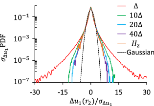
(b)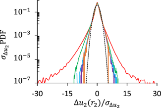
(c)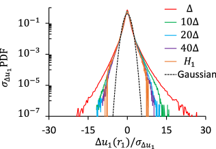
(d)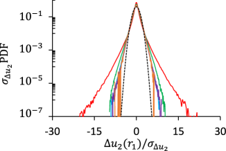
We note that while the PDFs of the velocity increments should asymptote to the single-point PDFs of the velocity in the limit , our data for the PDF of is very different (compare the left tails of the PDFs) from single-point PDF of shown in figure 6(a). This is probably simply due to the fact that, as already noted earlier the size of the FOV is not large enough for this asymptotic regime to be observed. The aforementioned PDFs are however so different that the flow behavior must undergo an interesting transition where negative fluctuations of the vertical velocity begin to be suppressed (but not positive fluctuations) as the scale continues to be increased. This point will be explored in a future work by employing a larger FOV to observe this asymptotic regime.
6.2 Flatness of velocity increment
(a)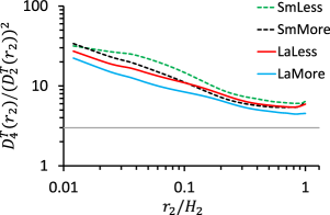
(b)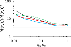
(c)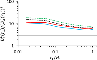
(d)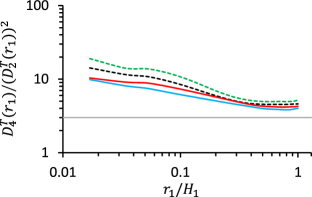
The intermittency and non-Gaussianity can be quantified using the flatness measures defined as (figure 16a,d) and (figure 16b,c). The first observation from the results in figure 16 is that the all four bubble-laden cases show a rather similar behaviour as increases, slowly reducing from values of up to 40 towards the Gaussian value of 3. However, there is still considerable deviation from 3 even at the largest scale , consistent with the PDF results for in figure 15. We also find that for both the transverse or longitudinal flatness measures and along either separations directions, the flatness is largest for the case with smaller , reflecting the same trend as the PDFs of the velocity increments at the single scale (figure 14). The values and behavior of the flatness are similar to those observed in Ma et al. (2021) for the three bubble-laden cases with , although for the present flow the flatness values are larger than those in Ma et al. (2021). For separations , the transverse flatness values are larger than the longitudinal ones, similar to what is observed in isotropic turbulence (Ishihara et al., 2009; Li & Meneveau, 2005). By contrast, for separations , the transverse flatness values are slightly smaller than the longitudinal ones.
6.3 Flow structures associated with extreme fluctuations
We now use flow visualization to understand which regions of the flow are associated with the extreme velocity increments. Figure 17(c,d) give two examples of such flow visualization extracted from a randomly chosen (but representative) FOV result for for the cases SmMore and LaMore, respectively. Each grid in the figure corresponds to an interrogation window of the present PSV. For convenience, we also plot in (a,b) the corresponding original velocity vector fields and denote in each case the in-focus bubbles. The images show that for both cases the regions where the velocity increment takes on extreme values are located in the outer-most region of the individual bubble wakes, while the fluctuations inside the wakes are relatively weak (see c,d). At a result of this it appears that the small-scale intermittency in the present flow already characterized is quite different from the small-scale intermittency that occurs in single-phase turbulence that arises due to nonlinear self amplification of the velocity gradients (Tsinober, 2001; Li & Meneveau, 2005; Buaria et al., 2019, 2020). In particular, the intermittency in the present flow is more similar to what is often called external intermittency (Townsend, 1949), which arises near the interface between two regions of the flow with significantly differing behavior, e.g. such as at the turbulent/non-turbulent interface in turbulent jets (da Silva et al., 2014; Gauding et al., 2021). In the bubble-laden flow we are considering, the intermittency arises at the interface between the edge of the bubble wake and the surrounding relatively quiescent flow.
(a)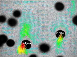
(b)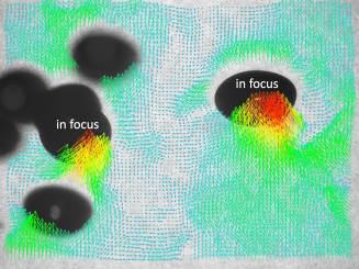
(c)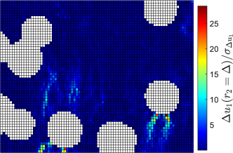
(d)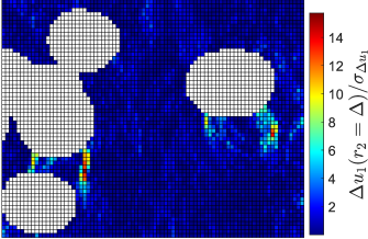
One further observation on figure 17(c,d) is that the extreme values are larger for the smaller bubble wakes than the larger bubble wakes (note the different legend scales in c,d). This point is made clearer in figure 18(a,b) where instead is plotted. Looking at the in-focus bubble on the right-hand side for both cases (where a more complete wake structure is visible than for the left in-focus bubble), we find that the regions of extreme values are larger for the SmMore case. By increasing the threshold to (figure 18c,d), we see that there are still some locations with extreme values satisfying this threshold for the SmMore, while there are none for the LaMore case. Although this observation is only for one snapshot, we have conducted the same analysis for many different snapshots and virtually all of them show the same behaviour. These observations are consistent with the PDF results in figure 14 that show that cases with smaller bubbles (lower ) have heavier tails than the cases with larger bubbles (higher ).
An explanation for why the intermittency is largest for the cases with smaller bubbles and lower volume fractions was given in Ma et al. (2021). When the volume fraction is not too large (but still large enough for the bubbles to make a statistically significant contribution to the flow properties), there are relatively few regions in the flow where turbulence is produced due to the bubble wakes, meaning that turbulence in the flow is very patchy and therefore intermittent. As the volume fraction increases, the regions of the flow influenced by the bubble wakes becomes less rare, and hence intermittency in the flow reduces. This then explains why the SmLess case is the most intermittent, and the LaMore case the least intermittent. Moreover, since the flow we are considering has no background turbulence (i.e. the only turbulence in the flow is the result of the bubble wakes), then this may explain why the intermittency we see is higher than that in Ma et al. (2021) where the flow considered had background turbulence, so that turbulent activity in the flow was not restricted to regions close to the bubbles.
(a)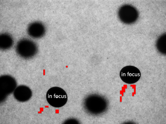
(b)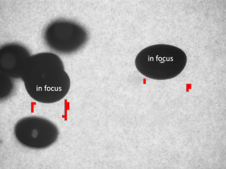
(c)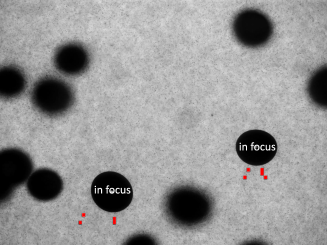
(d)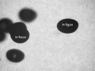
7 Conclusions
In this paper we have presented an analysis of the multiscale properties of a bubble-laden turbulent flow, based on experimental data of a flow in a vertical column with bubble swarms rising in water. The experiment takes advantage of a recently developed PSV technique for particle/bubble flows and provides the first comprehensive data set for computing multipoint measurements (without having to invoke Taylor’s hypothesis, in contrast to, e.g. Rensen et al. (2005)) of flows laden with finite-sized bubbles. By acquiring a very large number of snapshots of the velocity field we are able to compute structure functions of up to twelfth orders, and PDFs that resolve the heavy tails associated with extreme fluctuations in the flow.
The results show that the level of anisotropy in the flow produced by the rising bubbles is strong in general, and not negligible at any scale in the flow. Moreover, the results show that (i) the differing behaviour of the second-order longitudinal and transverse structure functions when measured for separations in different directions shows that both velocity components and separation directions of the 2 dimensional data need to be considered in order to fully characterize the anisotropy of the flow; (ii) the bubble size and void fraction are both important parameters determining the amount of anisotropy in the flow; (iii) higher-order structure functions reveal greater anisotropy across the scales of the flow, such that extreme fluctuations in the flow are the most anisotropic.
Since the PSV data captures two-dimensional data, we were able to consider the energy transfer between scales for two separation directions in the flow. The results revealed a downscale energy transfer on average for horizontal separations, but an upscale energy transfer on average in the vertical direction. However, the horizontal energy transfer was much stronger than that in the vertical direction.
We also investigated extreme events in the flow by considering the normalized probability density functions of the velocity increments in the flow. The results showed that the probability of extreme fluctuations increases with decreasing scale, just as in single-phase turbulence. However, the results also showed that for a given scale the probability of extreme events decreased with increasing Reynolds number, contrary to what occurs in single-phase turbulence. To explore the origin of these extreme fluctuations in the bubble-laden flows, we visualized regions of extreme small-scale velocity increments in the FOV and observed that they are typically located at the boundary of the wakes produced by the bubbles. For the cases with smaller bubbles and lower void fractions, vast regions outside of the bubbles wakes exhibit weak fluctuations, and so this combined with the extreme fluctuations at the bubble wake boundaries leads to strong intermittency. For larger bubbles which produce larger flow Reynolds numbers, and with larger void fractions, the wake regions become less rare in the flow and hence the flow is less intermittent than the former case, even though the Reynolds number is higher. Furthermore, the extreme values were also observed to reach larger values (compared to the standard deviation) for the smaller bubbles, which again causes the smaller bubble cases to exhibit greater intermittency than the larger bubble cases, in addition to the effect arising from the fraction of the flow modified by the bubble wakes.
Finally, it is worth pointing out two limitations with the present PSV data. First, the FOV is not large enough to resolve the integral length scales of the flow, and therefore as discussed in § 6.1 we were not able to fully resolve the transition in the properties of the bubble-laden flow as the scale approaches the intergral length scale. Second, the bubbles considered here all have approximately fixed shape, mimicking in nature small bubbles in a contaminated flow. We are currently performing new experiments with deformable bubbles and differing FOVs in order to address these two points and will report the results in future work.
Acknowledgements
The authors would like to acknowledge Thomas Ziegenhein for providing some routines for calculating bubble statistics. We also thank Ronald Franz and Uwe Hampel for providing the high-speed camera used in the present study.
Funding
T.M. acknowledges funding by Deutsche Forschungsgemeinschaft (DFG, German Research Foundation) under Grants MA 8408/1-1 and MA 8408/2-1.
Declaration of Interests
The authors report no conflict of interest.
Data availability
The data that support the findings of this study are available from the first author T.M. on request.
References
- Alexakis & Biferale (2018) Alexakis, A. & Biferale, L. 2018 Cascades and transitions in turbulent flows. Phys. Rep. 767, 1–101.
- Alméras et al. (2017) Alméras, E., Mathai, V., Lohse, D. & Sun, C. 2017 Experimental investigation of the turbulence induced by a bubble swarm rising within incident turbulence. J. Fluid Mech. 825, 1091–1112.
- Alméras et al. (2019) Alméras, E., Mathai, V., Sun, C. & Lohse, D. 2019 Mixing induced by a bubble swarm rising through incident turbulence. Int. J. Multiphase Flow 114, 316–322.
- Arad et al. (1999) Arad, I., L’vov, V. S. & Procaccia, I. 1999 Correlation functions in isotropic and anisotropic turbulence: The role of the symmetry group. Phys. Rev. E 59 (6), 6753.
- Balachandar & Eaton (2010) Balachandar, S. & Eaton, J. K. 2010 Turbulent dispersed multiphase flow. Annu. Rev. Fluid Mech. 42, 111–33.
- Banerjee et al. (2007) Banerjee, S, Krahl, R, Durst, F & Zenger, Ch 2007 Presentation of anisotropy properties of turbulence, invariants versus eigenvalue approaches. J. Turbul. 8, N32.
- Bec et al. (2006) Bec, J., Biferale, L., Boffetta, G., Celani, A., Cencini, M., Lanotte, A. S., Musacchio, S. & Toschi, F. 2006 Acceleration statistics of heavy particles in turbulence. J. Fluid Mech. 550, 349–358.
- Bec et al. (2007) Bec, J., Biferale, L., Cencini, M., Lanotte, A. S., Musacchio, S. & Toschi, F. 2007 Heavy particle concentration in turbulence at dissipative and inertial scales. Phys. Rev. Lett 98, 084502.
- Benzi et al. (1993) Benzi, R., Ciliberto, S., Tripiccione, R., Baudet, C., Massaioli, F. & Succi, S. 1993 Extended self-similarity in turbulent flows. Phys. Rev. E 48, R29–R32.
- Berk & Coletti (2021) Berk, T. & Coletti, F. 2021 Dynamics of small heavy particles in homogeneous turbulence: a lagrangian experimental study. J. Fluid Mech. 917, A47.
- Biferale et al. (2012) Biferale, L, Perlekar, P, Sbragaglia, M & Toschi, F 2012 Convection in multiphase fluid flows using lattice boltzmann methods. Phys. Rev. Lett. 108 (10), 104502.
- Biferale & Procaccia (2005) Biferale, L. & Procaccia, I. 2005 Anisotropy in turbulent flows and in turbulent transport. Phys. Rep. 414 (2-3), 43–164.
- Bourdon et al. (2006) Bourdon, Christopher J, Olsen, Michael G & Gorby, Allen D 2006 The depth of correlation in micro-PIV for high numerical aperture and immersion objectives. J. Fluids Eng. Trans. ASME 128.
- Bragg et al. (2021) Bragg, A. D., Liao, Y., Fröhlich, J. & Ma, T. 2021 Assessment of the validity of a log-law for wall-bounded turbulent bubbly flows. Int. J. Heat Fluid Flow in press.
- Bröder & Sommerfeld (2007) Bröder, D & Sommerfeld, M 2007 Planar shadow image velocimetry for the analysis of the hydrodynamics in bubbly flows. Measurement Science and Technology 18 (8), 2513.
- Buaria et al. (2020) Buaria, D., Bodenschatz, E. & Pumir, A. 2020 Vortex stretching and enstrophy production in high reynolds number turbulence. Phys. Rev. Fluids 5, 104602.
- Buaria et al. (2019) Buaria, D., Pumir, A., Bodenschatz, E. & Yeung, P. K. 2019 Extreme velocity gradients in turbulent flows. New Journal of Physics 21 (4), 043004.
- Carter & Coletti (2017) Carter, D. W & Coletti, F. 2017 Scale-to-scale anisotropy in homogeneous turbulence. J. Fluid Mech. 827, 250–284.
- Chang et al. (2012) Chang, K., Bewley, G. P. & Bodenschatz, E. 2012 Experimental study of the influence of anisotropy on the inertial scales of turbulence. J. Fluid Mech. 692, 464–481.
- Davidson (2015) Davidson, P. A. 2015 Turbulence: an introduction for scientists and engineers. Oxford university press.
- Dou et al. (2018a) Dou, Z., Bragg, A. D., Hammond, A. L., Liang, Z., Collins, L. R. & Meng, H. 2018a Effects of reynolds number and stokes number on particle-pair relative velocity in isotropic turbulence: a systematic experimental study. J. Fluid Mech. 839, 271–292.
- Dou et al. (2018b) Dou, Z., Ireland, P., Bragg, A.D., Ling, Z., Collins, L.R. & Meng, H. 2018b Particle-pair relative velocity measurement in high-reynolds-number homogeneous and isotropic turbulence using 4-frame particle tracking velocimetry. Experiments in Fluids 59.
- Elghobashi (2019) Elghobashi, S. 2019 Direct numerical simulation of turbulent flows laden with droplets or bubbles. Annu. Rev. Fluid Mech. 51 (1), 217–244.
- Estevadeordal & Goss (2005) Estevadeordal, Jordi & Goss, Larry 2005 PIV with LED: particle shadow velocimetry (PSV) technique. In 43rd AIAA aerospace sciences meeting and exhibit, p. 37.
- Fox (2014) Fox, R. O. 2014 On multiphase turbulence models for collisional fluid-particle flows. J. Fluid Mech. 742, 368–424.
- Frisch (1995) Frisch, U. 1995 Turbulence: the legacy of AN Kolmogorov. Cambridge university press.
- Gauding et al. (2021) Gauding, M, Bode, M, Brahami, Y, Varea, É & Danaila, L 2021 Self-similarity of turbulent jet flows with internal and external intermittency. J. Fluid Mech. 919.
- Gotoh et al. (2002) Gotoh, T., Fukayama, D. & Nakano, T. 2002 Velocity field statistics in homogeneous steady turbulence obtained using a high-resolution direct numerical simulation. Phys. Fluids 14 (3), 1065–1081.
- Gustavsson & Mehlig (2016) Gustavsson, K. & Mehlig, B. 2016 Statistical models for spatial patterns of heavy particles in turbulence. Advances in Physics 65 (1), 1–57.
- Harteveld et al. (2003) Harteveld, W. K., Mudde, R. F. & van den Akker, H. E. A. 2003 Dynamics of a bubble column: influence of gas distribution on coherent structures. Can. J. Chem. Eng. 81 (3-4), 389–394.
- Hessenkemper & Ziegenhein (2018) Hessenkemper, H & Ziegenhein, T 2018 Particle shadow velocimetry (PSV) in bubbly flows. Int. J. Multiphase Flow 106, 268–279.
- Hessenkemper et al. (2021) Hessenkemper, H, Ziegenhein, T & Lucas, D. 2021 Using neural networks for segmantic segmentation of overlapping bubbles in bubbly flows. In preperation .
- Hill (2001) Hill, R. J. 2001 Equations relating structure functions of all orders. J. Fluid Mech. 434, 379–388.
- Hogendoorn & Poelma (2018) Hogendoorn, Willian & Poelma, Christian 2018 Particle-laden pipe flows at high volume fractions show transition without puffs. Phys. Rev. Lett. 121, 194501.
- Innocenti et al. (2021) Innocenti, A., Jaccod, A., Popinet, S. & Chibbaro, S. 2021 Direct numerical simulation of bubble-induced turbulence. J. Fluid Mech. 918.
- Ireland et al. (2016a) Ireland, P.J., Bragg, A.D. & Collins, L.R. 2016a The effect of reynolds number on inertial particle dynamics in isotropic turbulence. part 1. simulations without gravitational effects. J. Fluid Mech. 796, 617–658.
- Ireland et al. (2016b) Ireland, P. J., Bragg, A. D. & Collins, L. R. 2016b The effect of reynolds number on inertial particle dynamics in isotropic turbulence. part 2. simulations with gravitational effects. J. Fluid Mech. 796, 659–711.
- Ishihara et al. (2009) Ishihara, T., Gotoh, T. & Kaneda, Y. 2009 Study of high–reynolds number isotropic turbulence by direct numerical simulation. Annu. Rev. Fluid Mech. 41, 165–180.
- Kolmogorov (1941) Kolmogorov, A. N. 1941 The local structure of turbulence in incompressible viscous fluid for very large reynolds numbers. Dokl. Akad. Nauk SSSR 30, 299–303.
- Kurien & Sreenivasan (2000) Kurien, S. & Sreenivasan, K. R. 2000 Anisotropic scaling contributions to high-order structure functions in high-reynolds-number turbulence. Phys. Rev. E 62 (2), 2206.
- Lai & Socolofsky (2019) Lai, C. C. K. & Socolofsky, S. A. 2019 The turbulent kinetic energy budget in a bubble plume. J. Fluid Mech. 865, 993–1041.
- Lance & Bataille (1991) Lance, M. & Bataille, J. 1991 Turbulence in the liquid phase of a uniform bubbly air-water flow. J. Fluid Mech. 222, 95–118.
- Li & Meneveau (2005) Li, Y. & Meneveau, C. 2005 Origin of non-gaussian statistics in hydrodynamic turbulence. Phys. Rev. Lett. 95 (16), 164502.
- Liao & Lucas (2010) Liao, Y. & Lucas, D. 2010 A literature review on mechanisms and models for the coalescence process of fluid particles. Chemical Engineering Science 65 (10), 2851–2864.
- Lohse (2018) Lohse, D. 2018 Bubble puzzles: From fundamentals to applications. Phys. Rev. Fluids 3 (11), 110504.
- Lu & Tryggvason (2008) Lu, J. & Tryggvason, G. 2008 Effect of bubble deformability in turbulent bubbly upflow in a vertical channel. Phys. Fluids 20, 040701.
- Lu & Tryggvason (2013) Lu, J. & Tryggvason, G. 2013 Dynamics of nearly spherical bubbles in a turbulent channel upflow. J. Fluid Mech. 732, 166–189.
- Ma et al. (2020a) Ma, T., Lucas, D. & Bragg, A. D 2020a Explicit algebraic relation for calculating reynolds normal stresses in flows dominated by bubble-induced turbulence. Phys. Rev. Fluids 5, 084305.
- Ma et al. (2020b) Ma, T., Lucas, D., Jakirlić, S. & Fröhlich, J. 2020b Progress in the second-moment closure for bubbly flow based on direct numerical simulation data. J. Fluid Mech. 883, A9.
- Ma et al. (2021) Ma, T., Ott, B., Fröhlich, J. & Bragg, A. D 2021 Scale-dependent anisotropy, energy transfer and intermittency in bubble-laden turbulent flows. J. Fluid Mech. in press.
- Ma et al. (2017) Ma, T., Santarelli, C., Ziegenhein, T., Lucas, D. & Fröhlich, J. 2017 Direct numerical simulation-based Reynolds-averaged closure for bubble-induced turbulence. Phys. Rev. Fluids 2, 034301.
- Maeda et al. (2021) Maeda, K., Date, M., Sugiyama, K., Takagi, S. & Matsumoto, Y. 2021 Viscid–inviscid interactions of pairwise bubbles in a turbulent channel flow and their implications for bubble clustering. J. Fluid Mech. 919, A30.
- Magnaudet & Eames (2000) Magnaudet, J. & Eames, I. 2000 The motion of high-reynolds-number bubbles in inhomogeneous flows. Annu. Rev. Fluid Mech. 32 (1), 659–708.
- Manikantan & Squires (2020) Manikantan, H. & Squires, T. M 2020 Surfactant dynamics: hidden variables controlling fluid flows. J. Fluid Mech. 892, P1.
- Masuk et al. (2021a) Masuk, A. U. M., Qi, Y., Salibindla, A. K. R. & Ni, R. 2021a Towards a phenomenological model on the deformation and orientation dynamics of finite-sized bubbles in both quiescent and turbulent media. J. Fluid Mech. 920, A4.
- Masuk et al. (2021b) Masuk, A. U. M., Salibindla, A. K. R. & Ni, R. 2021b Simultaneous measurements of deforming hinze-scale bubbles with surrounding turbulence. J. Fluid Mech. 910, A21.
- Mathai et al. (2020) Mathai, V., Lohse, D. & Sun, C. 2020 Bubbly and buoyant particle–laden turbulent flows. Annu. Rev. Condens. Matter Phys. 11 11, 529–559.
- Maxey (1987) Maxey, M. R. 1987 The gravitational settling of aerosol particles in homogeneous turbulence and random flow fields. J. Fluid Mech. 174, 441–465.
- Mendez-Diaz et al. (2013) Mendez-Diaz, S., Serrano-García, J. C., Zenit, R. & Hernández-Cordero, J. A. 2013 Power spectral distributions of pseudo-turbulent bubbly flows. Phys. Fluids 25 (4).
- Mudde (2005) Mudde, R. F. 2005 Gravity-driven bubbly flows. Annu. Rev. Fluid Mech. 37, 393–423.
- Ouellette et al. (2006) Ouellette, N. T., Xu, H., Bourgoin, M. & Bodenschatz, E. 2006 Small-scale anisotropy in lagrangian turbulence. New J. Phys. 8 (6), 102.
- Pandey et al. (2020) Pandey, V., Ramadugu, R. & Perlekar, P. 2020 Liquid velocity fluctuations and energy spectra in three-dimensional buoyancy-driven bubbly flows. J. Fluid Mech. 884, R6.
- Perrard et al. (2021) Perrard, S., Rivière, A., Mostert, W. & Deike, L. 2021 Bubble deformation by a turbulent flow. J. Fluid Mech. 920.
- Petersen et al. (2019) Petersen, A. J., Baker, L. & Coletti, F. 2019 Experimental study of inertial particles clustering and settling in homogeneous turbulence. J. Fluid Mech. 864, 925–970.
- Pope (2000) Pope, S. B. 2000 Turbulent Flows, 1st edn. Cambridge University Press.
- Prakash et al. (2016) Prakash, V. N., Mercado, J. M., van Wijngaarden, L., Mancilla, E., Tagawa, Y., Lohse, D. & Sun, C. 2016 Energy spectra in turbulent bubbly flows. J. Fluid Mech. 791, 174–190.
- Prosperetti & Tryggvason (2009) Prosperetti, A. & Tryggvason, G. 2009 Computational Methods for Multiphase Flow. Cambridge University Press.
- Pumir & Shraiman (1995) Pumir, A. & Shraiman, B. I. 1995 Persistent small scale anisotropy in homogeneous shear flows. Phys. Rev. Lett. 75 (17), 3114.
- Pumir et al. (2016) Pumir, A., Xu, H. & Siggia, E. D. 2016 Small-scale anisotropy in turbulent boundary layers. J. Fluid Mech. 804, 5–23.
- Rensen et al. (2005) Rensen, J., Luther, S. & Lohse, D. 2005 The effect of bubbles on developed turbulence. J. Fluid Mech. 538, 153–187.
- Riboux et al. (2010) Riboux, G., Risso, F. & Legendre, D. 2010 Experimental characterization of the agitation generated by bubbles rising at high Reynolds number. J. Fluid Mech. 643, 509–539.
- Risso (2018) Risso, F. 2018 Agitation, mixing, and transfers induced by bubbles. Annu. Rev. Fluid Mech. 50, 25–48.
- Rivière et al. (2021) Rivière, A., Mostert, W., Perrard, S. & Deike, L. 2021 Sub-hinze scale bubble production in turbulent bubble break-up. J. Fluid Mech. 917.
- Roghair et al. (2011) Roghair, I., Mercado, J. M., Van Sint Annaland, M., Kuipers, H., Sun, C. & Lohse, D. 2011 Energy spectra and bubble velocity distributions in pseudo-turbulence: Numerical simulations vs. experiments. Int. J. Multiphase Flow 37, 1093–1098.
- Ronneberger et al. (2015) Ronneberger, O., Fischer, P. & Brox, T. 2015 U-net: Convolutional networks for biomedical image segmentation. In International Conference on Medical image computing and computer-assisted intervention, pp. 234–241. Springer.
- Santarelli et al. (2016) Santarelli, C., Roussel, J. & Fröhlich, J. 2016 Budget analysis of the turbulent kinetic energy for bubbly flow in a vertical channel. Chem. Eng. Sci. 141, 46–62.
- Sapsis (2021) Sapsis, T. P. 2021 Statistics of extreme events in fluid flows and waves. Annu. Rev. Fluid Mech. 53, 85–111.
- Shen & Warhaft (2000) Shen, X & Warhaft, Z 2000 The anisotropy of the small scale structure in high reynolds number () turbulent shear flow. Phys. Fluids 12 (11), 2976–2989.
- da Silva et al. (2014) da Silva, C. B., Hunt, J. C. R., Eames, I. & Westerweel, J. 2014 Interfacial layers between regions of different turbulence intensity. Annu. Rev. Fluid Mech. 46, 567–590.
- Sreenivasan & Antonia (1997) Sreenivasan, K. R. & Antonia, R. A. 1997 The phenomenology of small-scale turbulence. Annu. Rev. Fluid Mech. 29 (1), 435–472.
- Tagawa et al. (2014) Tagawa, Y., Takagi, S. & Matsumoto, Y. 2014 Surfactant effect on path instability of a rising bubble. J. Fluid Mech. 738, 124.
- Takagi & Matsumoto (2011) Takagi, S. & Matsumoto, Y. 2011 Surfactant effects on bubble motion and bubbly flows. Annu. Rev. Fluid Mech. 43, 615–636.
- Tom & Bragg (2019) Tom, J. & Bragg, A. D. 2019 Multiscale preferential sweeping of particles settling in turbulence. J. Fluid Mech. 871, 244–270.
- Townsend (1949) Townsend, A. 1949 The fully developed wake of a circular cylinder. Aust. J. Chem. 2 (4), 451–468.
- Tropea (2011) Tropea, C. 2011 Optical particle characterization in flows. Annu. Rev. Fluid Mech. 43, 399–426.
- Tsinober (2001) Tsinober, A. 2001 An informal introduction to turbulence. Kluwer Academic Publishers.
- Warhaft & Shen (2002) Warhaft, Z & Shen, X 2002 On the higher order mixed structure functions in laboratory shear flow. Phys. Fluids 14 (7), 2432–2438.
- Wereley & Meinhart (2010) Wereley, S. T. & Meinhart, C. D. 2010 Recent advances in micro-particle image velocimetry. Annu. Rev. Fluid Mech. 42, 557–576.
- Yeung et al. (2015) Yeung, P. K., Zhai, X. M. & Sreenivasan, K. R. 2015 Extreme events in computational turbulence. Proc. Natl. Acad. Sci. 112 (41), 12633–12638.
- Zenit et al. (2001) Zenit, R., Koch, D. L. & Sangani, A. S. 2001 Measurements of the average properties of a suspension of bubbles rising in a vertical channel. J. Fluid Mech. 429, 307–342.
- Ziegenhein & Lucas (2016) Ziegenhein, T. & Lucas, D. 2016 On sampling bias in multiphase flows: Particle image velocimetry in bubbly flows. Flow Measurement and Instrumentation 48, 36–41.