Weighted Low Rank Matrix Approximation and Acceleration

Abstract

Low-rank matrix approximation is one of the central concepts in machine learning, with applications in dimension reduction, de-noising, multivariate statistical methodology, and many more. A recent extension to LRMA is called low-rank matrix completion (LRMC). It solves the LRMA problem when some observations are missing and is especially useful for recommender systems. In this paper, we consider an element-wise weighted generalization of LRMA. The resulting weighted low-rank matrix approximation technique therefore covers LRMC as a special case with binary weights. WLRMA has many applications. For example, it is an essential component of GLM optimization algorithms, where an exponential family is used to model the entries of a matrix, and the matrix of natural parameters admits a low-rank structure. We propose an algorithm for solving the weighted problem, as well as two acceleration techniques. Further, we develop a non-SVD modification of the proposed algorithm that is able to handle extremely high-dimensional data. We compare the performance of all the methods on a small simulation example as well as a real-data application.

Keywords: low-rank approximation, matrix completion, soft-impute, alternating least squares

1 Introduction and background

1.1 Low-rank matrix approximation

Low-rank matrix approximation (LRMA) has always attracted a lot of attention. It arises in a variety of core machine learning techniques including data compression, dimension reduction and de-noising (Markovsky, 2011), and is central to many multivariate statistical techniques such as principal components, linear discriminant analysis and canonical correlation analysis (Mardia et al., 1979). The main goal of the LRMA technique is to identify the “best” way to approximate some given matrix $M\in\mathbb{R}^{n\times p}$ with a rank-$k$ matrix $X\in\mathbb{R}^{n\times p}$ for $k<\min(n,p)$. There are many ways to define “goodness of fit” between a matrix and its approximation. The most natural one is to use the residual sum of squares $\sum_{i=1}^{n}\sum_{j=1}^{p}(M_{ij}-~{}X_{ij})^{2}$ leading to the LMRA problem:

$$\operatornamewithlimits{minimize}_{X\in\mathbb{R}^{n\times p}}\|M-X\|^{2}_{F}\quad\mbox{ subject to }\operatorname{rk}(X)\leq k.$$ (1)

Here $\|\cdot\|_{F}$ refers to Frobenius norm. The solution to this problem is well-know and can be found via the singular value decomposition (SVD) of the matrix $M$ (Eckart & Young, 1936).

1.2 Missing values

The LRMA problem can be extended to the case when only a subset of entries in $M$ is observed. The resulting technique, also known as low-rank matrix completion (LRMC), aims to recover the missing entries of matrix $M$ from partial observations (Candès & Recht, 2008; Mazumder et al., 2010; Nguyen et al., 2019). One of the most famous examples of widespread use of LRMC is the “Netflix” competition, where the goal is to build a movie recommendation system based on users ratings of movies they have seen (Feuerverger et al., 2012). Here $M$ is the matrix of movie ratings (score from one to five), where each column represents a movie, each row represents a user, and most elements in $M$ are missing. We seek a low-rank matrix $X$ that approximates the observed entries of $M$ well, and can be used to fill in the missing values. The low-rank structure has a heuristic justification in terms of “cliques” of users and “genres” of movies.

Following Candes & Tao (2010), to state the corresponding optimization problem one denotes a set of observed entries by $\Omega\in\{1,\ldots,n\}\times\{1,\ldots,p\}$ and defines the projection operator $P_{\Omega}:\mathbb{R}^{n\times p}\to\mathbb{R}^{n\times p}$ as follows

$$(P_{\Omega}(X))_{ij}=\begin{cases}0,\mbox{ if }(i,j)\notin\Omega\\ X_{ij},\mbox{ if }(i,j)\in\Omega.\end{cases}$$

In other words, the projection operator replaces all missing elements by zeroes. The LRMC problem becomes

$$\operatornamewithlimits{minimize}_{X\in\mathbb{R}^{n\times p}}\|P_{\Omega}(M-X)\|^{2}_{F}\quad\mbox{ subject to }\operatorname{rk}(X)\leq k.$$ (2)

The objective in (2) is nothing but the residual sum of squares computed for the set of observed values only, i.e. $\sum_{(i,j)\in\Omega}(M_{ij}-~{}X_{ij})^{2}$. Unlike the complete matrix case, where an explicit solution exists, LRMC requires an iterative algorithm. Hard-impute is an example of such an algorithm, and alternates two steps: the imputation step, where the current guess for $X$ is used to complete the unobserved entries in $M$; and the SVD step which updates the low-rank matrix approximation $X$ (Mazumder et al., 2010).

Note that problem (2) is non-convex, which makes it hard to establish a formal proof of convergence of the algorithm. A natural convex relaxation of the LRMC problem can be stated as follows (Mazumder et al., 2010; Candes & Tao, 2010):

$$\operatornamewithlimits{minimize}_{X\in\mathbb{R}^{n\times m}}\frac{1}{2}\|P_{\Omega}(M-X)\|^{2}_{F}+\lambda\|X\|_{*}$$ (3)

Here $\|\cdot\|_{*}$ refers to the nuclear norm of a matrix (sum of singular values) and is a convex relaxation of the matrix rank function. The iterative algorithm solving (3) is called soft-impute. It is essentially the same as hard-impute, but instead of truncating some eigenvalues to zero at the second step (i.e. computing low-rank approximation) they are shrunk via a soft-thresholding operator (Mazumder et al., 2010). There is a link between problem (2) and its convex relaxation. Since shrinking its nuclear norm is a smooth way to reduce the rank of a matrix, then for $\lambda$ large enough problem (3) will produce a rank $k$ solution.

An alternative view of LRMA was suggested by Rennie & Srebro (2005). One can show that any rank $k$ matrix $X\in\mathbb{R}^{n\times p}$ can be rewritten as $X=AB^{\top},$ where $A\in~{}\mathbb{R}^{n\times k},B\in\mathbb{R}^{p\times k}.$ Restating problem (2) in terms of $A$ and $B$ leads to an equivalent bi-convex problem:

$$\operatornamewithlimits{minimize}_{A\in\mathbb{R}^{n\times k},B\in\mathbb{R}^{p\times k}}\|P_{\Omega}(M-AB^{\top})\|^{2}_{F}$$ (4)

For the convex relaxation the following result holds: if $r$ is the rank of the solution to problem (3), then for any $k>r$ problem (3) is equivalent to

$$\operatornamewithlimits{minimize}_{A\in\mathbb{R}^{n\times k},B\in\mathbb{R}^{p\times k}}\frac{1}{2}\|P_{\Omega}(M-AB^{\top})\|^{2}_{F}+\frac{\lambda}{2}\|A\|^{2}_{F}+\frac{\lambda}{2}\|B\|_{F}^{2}$$ (5)

Hastie et al. (2015) suggest an efficient alternating least squares algorithm for solving problem (5).

1.3 Weighted generalization

In this paper we focus on a weighted generalization of LRMA. There are many applications of WLRMA beyond matrix completion. In Ecology, Robin et al. (2019) and Łukasz Kidziński et al. (2020) propose modelling populations of species using Poisson GLMs. The authors analyse the population matrices (with rows and columns corresponding to sites and species, respectively) using low-rank models. As a result, they develop an iterative algorithm that solves a matrix-type Poisson GLM optimization problem with a low-rank constraint. The algorithm is based on Newton descent where each Newtons step can be restated in the form of a WLRMA problem.

In Tuzhilina et al. (2020) the authors build a technique for chromatin conformation reconstruction. They model the so-called contact matrix, which represents the frequency of contacts between each pair of genomic loci, via a Poisson distribution and link mean contact counts to the pairwise distances between loci. The low-rank constraint is natural here, since chromatin is a 3D structure; in addition the authors model chromatin as a smooth curve. The resulting optimization problem can be solved via an iterative algorithm, where each iteration is equivalent to solving a WLRMA problem.

Note that the projection operator introduced in the previous section is equivalent to multiplying each element of a matrix either by zero (for unobserved entries) or by one (for observed entries). In other words, $P_{\Omega}(X)$ can be rewritten as $W*X$, where $W\in\mathbb{R}^{n\times p}$ is a binary matrix with

$$W_{ij}=~{}\begin{cases}0,\mbox{ if }(i,j)\notin\Omega\\ 1,\mbox{ if }(i,j)\in\Omega\end{cases}$$

and $*$ refers to the Hadamard element-wise product. The natural generalization of the LRMC problem is therefore

$$\operatornamewithlimits{minimize}_{X\in\mathbb{R}^{n\times p}}\|\sqrt{W}*(M-X)\|_{F}^{2}\quad\mbox{subject to }\operatorname{rk}(X)\leq k.$$ (6)

Here $W\in[0,1]^{n\times p}$ is a matrix of weights (not necessary binary) and the objective is simply weighted residual sum of squares $\sum_{i=1}^{n}\sum_{j=1}^{p}W_{ij}(M_{ij}-~{}X_{ij})^{2}$.

Of course, there is a convex relaxation of problem (6), i.e.

$$\operatornamewithlimits{minimize}_{X\in\mathbb{R}^{n\times p}}\frac{1}{2}\|\sqrt{W}*(M-X)\|_{F}^{2}+\lambda\|X\|_{*}$$ (7)

The WLRMA problem was first introduced by Srebro & Jaakkola (2003) (see also Razenshteyn et al., 2016; Dutta et al., 2018; Ban et al., 2019). Originally the authors suggested a simple iterative algorithm that successively replaces the current guess of $X$ by a low-rank-matrix approximation of $W*M+(1-W)*X$. This iterative procedure has a natural interpretation: you first “blend” your current guess for $X$ with the ground truth $M$ (using weights $W$ and $1-W$) and then project the combination back to the manifold of rank-$k$ matrices. With a matrix of binary weights, this procedure coincides with the hard-impute approach discussed above.

This paper is organized as follows. In Section 2 we link the existing WLRMA approach (hereafter we call it baseline) as well as the soft- and hard-impute algorithms to projected gradient descent. In Section 3.1 we use this link to propose an acceleration technique for the baseline method based on Nesterov acceleration. Further we provide an alternative way to improve the speed of WLRMA convergence: we restate the original problem as a fixed point equation and combine projected gradient descent with Anderson acceleration. We discuss these ideas as well as the way to stabilize the convergence behavior of Anderson acceleration in Sections 3.2 and 5. All of the proposed algorithms require us to compute an SVD at each iteration, which is computationally expensive in high-dimensions. In Section 6 we discuss an adaptation of the proposed techniques to the high-dimensional data setting. Finally, we demonstrate and compare the performance of all the methods on a simulation example as well as a real-data example from recomendataion systems (see Sections 4 and 7). When we finished writing this paper we discovered a recent preprint, which shares some of the ideas we propose in Sections 3.1 and 6 (Dutta et al., 2021).

2 Link to proximal gradient descent

In this section we link the WLRMA algorthm proposed in Srebro & Jaakkola (2003) to proximal gradient descent. This connection will subsequently help us to develop several useful algorithmic extensions. Note that the same link can be established for the convex relaxation of the WLRMA problem, as well as the soft- and hard-impute approaches.

Proximal gradient descent (PGD) is a method that allows one to solve non-differentiable convex optimization problems (Combettes & Wajs, 2005; Combettes & Pesquet, 2011). Specifically, suppose you aim to minimize $g(x)+h(x)$ w.r.t. $x\in\mathbb{R}^{d}$, where $g(x)$ is convex and differentiable and $h(x)$ is convex and not necessarily differentiable. For the non-differentiable part we define the proximal operator as follows:

$$\operatorname{prox}_{h}(x)=\operatorname{argmin}_{z}\frac{1}{2}\|x-z\|^{2}_{2}+h(z).$$

If $x^{(0)}$ refers to some initialization of $x$ and $x^{(i)}$ is the value of the optimized parameter at iteration $i$ then the proximal gradient descent update is

$$x^{(i+1)}:=\operatorname{prox}_{h}(x^{(i)}-\nabla g(x^{(i)})).$$

The update can be split in two parts: first the standard gradient step is done using the differentiable part of the objective, then the non-differentiable part is taken into account via proximal mapping.

Now we link PGD to the WLRMA problems (6) and (7). For the non-convex version we first restate problem (6) as follows:

$$\operatornamewithlimits{minimize}_{X\in\mathbb{R}^{n\times p}}\frac{1}{2}\|\sqrt{W}*(M-X)\|_{F}^{2}+\mathbbm{1}_{C}(X)$$

Here $C=\{X\in\mathbb{R}^{n\times p},~{}\operatorname{rk}(X)\leq k\}$ is the set of rank $k$ matrices and

$$\mathbbm{1}_{C}(X)=\begin{cases}0,\mbox{ if }X\in C,\\ \infty,\mbox{ if }X\notin C.\end{cases}$$

is the set indicator function. Since indicator is a non-differentiable function, we set $g(X)=\frac{1}{2}\|\sqrt{W}*(M-X)\|_{F}^{2}$ and $h(X)=\mathbbm{1}_{C}(X)$. It is not difficult to prove that the proximal operator of an indicator function of a set is just the projection onto this set (in the case of the set constraint the algorithm is therefore referred as Projected Gradient Descent). Further, note that projecting onto the set of rank $k$ matrices is equivalent to solving LRMA problem (1). Denote the rank $k$ approximation of matrix $X$ by $\mbox{SVD}_{k}(X)$, i.e. if $X=UDV^{\top}$ is the singular value decomposition then

$$\mbox{SVD}_{k}(X)=U\operatorname{diag}(d_{1},\ldots,d_{k},0,\ldots,0)V^{\top}.$$

Computing the gradient of the differential part of the objective, i.e.

$$\nabla g(X)=-W*(M-X),$$

we get the following PGD update for the WLRMA problem:

$$X^{(i+1)}:=\mbox{SVD}_{k}(W*M+(1-W)*X^{(i)}).$$ (8)

Although motivated by the EM algorithm, the update suggested in Srebro & Jaakkola (2003) coincides with the one we just derived via PGD.

Now let us consider the convex relaxation. Since in problem (7) the nuclear norm is a non-differentiable function of $X$, we set

$f(X)=\frac{1}{2}\|\sqrt{W}*(M-X)\|_{F}^{2}\mbox{ and }h(X)=\lambda\|X\|_{*}$.

One can show that proximal operator for $h(X)$ in this case is the soft-threshold operator (see, for example, Mazumder et al., 2010), i.e. $\operatorname{prox}_{C}(X)=\mbox{S}_{\lambda}(X)$ where

$$\mbox{S}_{\lambda}(X)=U\operatorname{diag}((d_{1}-\lambda)_{+},\ldots,(d_{p}-\lambda)_{+})V^{\top}.$$

and $x_{+}=\max(0,x)$ is the threshold operator. This leads us to the PGD update as follows:

$$X:=\mbox{S}_{\lambda}(W*M+(1-W)*X).$$ (9)

Similar to standard gradient descent, it is possible to add a learning rate $t$ to the PGD procedure leading to the hard and soft updates

$$X^{(i+1)} := \mbox{SVD}_{k}(tW*M+(1-tW)*X^{(i)})\mbox{ and}$$

$$X^{(i+1)} := \mbox{S}_{t\lambda}(tW*M+(1-tW)*X^{(i)})$$

respectively. Although optimizing the learning rate may improve convergence, it can be quite expensive to run line search in the context of WLRMA, as a separate SVD is required for each value of $t$.

3 Acceleration Techniques

There exist several ways to accelerate proximal gradient descent. We discuss two in this section: Nesterov and Anderson acceleration.

3.1 Nesterov

PGD can be combined with Nesterov acceleration, which uses momentum from previous iterations (Nesterov, 1983). Specifically, if we denote

$$V^{(i)}=X^{(i)}+\frac{i-1}{i+2}\left(X^{(i)}-X^{(i-1)}\right)$$ (10)

then the PGD procedure for both non-convex and convex versions of the WLRMA is as follows:

$$X^{(i+1)} :=\mbox{SVD}_{k}(W*M+(1-W)*V^{(i)})\mbox{ and }$$ (11)

$$X^{(i+1)} :=\mbox{S}_{\lambda}(W*M+(1-W)*V^{(i)}).$$ (12)

3.2 Anderson

Here we propose an alternative way to improve the convergence of the WLRMA baseline method via Anderson acceleration. To make it concise we present this technique for the non-convex WLRMA problem only. The same extension can be done for the convex relaxation as well.

Anderson acceleration (AA), or Anderson mixing, is a well-known method demonstrated to be very efficient for accelerating the convergence of fixed-point iterations (see, for example, Anderson, 1965; Walker & Ni, 2011; Zhang et al., 2020). It is similar in flavor to most acceleration methods which combine the previous updates of the optimized parameter to improve the convergence speed. Given some function $f(x):\mathbb{R}^{d}\to\mathbb{R}^{d}$, initialization $x^{(0)}$ and depth $m$, Anderson acceleration solves the fixed point equation $x=f(x)$ via the following steps:

1. Iteration $0$: set $x^{(1)}=f(x^{(0)})$.

2. Iteration $i=1,2,\ldots$:

   1. If $i<m$ we replace $m$ by $m_{*}=\min\{m,i\}$. This step is required only for the first few iterations.

   2. Store updates in a matrix $F^{(i)}=\left(f^{(i-m)},\ldots,f^{(i)}\right)$ where $f^{(j)}=f(x^{(j)})$.

   3. Store residuals in a matrix $R^{(i)}=\left(r^{(i-m)},\ldots,r^{(i)}\right)$ where $r^{(j)}=f^{(j)}-x^{(j)}$.

   4. Find coefficients $\alpha=(\alpha_{m},\ldots,\alpha_{0})^{\top}$ such that $\sum_{j=0}^{m}\alpha_{j}=1$ and that minimize the linear combination of residuals, i.e. $\|R^{(i)}\alpha\|_{2}$.

   5. Combine previous updates setting $x^{(i+1)}=F^{(i)}\alpha.$

Note that the optimization problem

$$\operatornamewithlimits{minimize}_{\alpha:\;\alpha^{\top}\mathbf{1}=1}\left\|R^{(i)}\alpha\right\|_{2}$$ (13)

has an explicit solution

$$\alpha^{*}=\frac{\left({R^{(i)}}^{\top}R^{(i)}\right)^{-1}\mathbf{1}}{\mathbf{1}^{\top}\left({R^{(i)}}^{\top}R^{(i)}\right)^{-1}\mathbf{1}}$$ (14)

which can be found in two steps. First we solve equation ${R^{(i)}}^{\top}R^{(i)}\theta=\mathbf{1}$ and then normalize the solution $\alpha=\frac{\theta}{\mathbf{1}^{\top}\theta}$.

To combine WLRA with Anderson acceleration we first need to restate the PGD procedure as a fixed point equation. Following the idea suggested in the recent paper by Mai & Johansson (2020) we restate the WLRA update as

$$Y^{(i+1)}=W*M+(1-W)*X^{(i)}\mbox{ and }X^{(i+1)}=\mbox{SVD}_{k}(Y^{(i+1)}).$$

Note that $Y^{(i)}$ is an update after the gradient step and in the case of binary weights it will simply represent the imputed matrix $M$. Then the convergence for the baseline WLRMA is guaranteed when the following fixed-point equation (written in terms of the auxiliary variable $Y$) holds

$$Y=f(Y)\mbox{ where }f(Y)=W*M+(1-W)*\mbox{SVD}_{k}(Y).$$

Note that in Anderson acceleration $x$ is assumed to be a vector and the WLRA problem is stated in matrix form, so in order to run Anderson acceleration in the context of WLRMA we need to vectorize all the matrices. We will use lower case letters to denote flattened matrices, e.g. $y=\operatorname{vec}(Y)$ and $f=\operatorname{vec}(f(Y))$. This leads us to the following implementation of the WLRMA-AA algorithm. In order to build similar algorithm for the convex relaxation one replace $\mbox{SVD}_{k}(\cdot)$ by $\mbox{S}_{\lambda}(\cdot)$.

Algorithm 1 WLRMA-Anderson

1. Initialize

   1. Initialize $Y^{(0)}$ (e.g. column mean imputation) and $y^{(0)}=\operatorname{vec}(Y^{{(0)}}).$

   2. Compute $X^{(0)}=\mbox{SVD}_{k}(Y^{(0)}).$

2. Repeat until convergence

   1. Compute $f^{(i)}=\operatorname{vec}(W*M+(1-W)*X^{(i)}).$

   2. Set $r^{(i)}=f^{(i)}-y^{(i)}$

   3. Concatenate $R^{(i)}=[R^{(i-1)}:r^{(i)}],~{}~{}~{}~{}F^{(i)}=[F^{(i-1)}:f^{(i)}].$

   4. Solve OLS:

      1. solve ${R^{(i)}}^{\top}R^{(i)}\theta=\mathbf{1}$ w.r.t. $\theta$,

      2. normalize $\alpha=\frac{\theta}{\mathbf{1}^{\top}\theta}$.

   5. Compute $y^{(i+1)}=F^{(i)}\alpha$ and set $Y^{(i+1)}=\operatorname{matrix}(y^{(i+1)})$.

   6. Update $X^{(i+1)}=\mbox{SVD}_{k}(Y^{(i+1)}).$

   7. Drop the first column of both $F^{(i)}$ and $R^{(i)}$ if they contain more than $m$ columns.

One can find a link between the proposed algorithm and Nesterov acceleration. First note that since $\sum_{i=0}^{m}\alpha_{i}=1$ the update for the auxiliary variable can be rewritten as:

$$Y^{(i+1)}=W*M+(1-W)*\sum_{j=0}^{m}\alpha_{j}X^{(i-j)}.$$ (15)

Thus if we denote

$$V^{(i)}=\sum_{j=0}^{m}\alpha_{j}X^{(i-j)},$$ (16)

which is nothing but some linear combination of previous $X$ updates, then step 2.6 in the above algorithm will coincide with the second step of the Nesterov update (12).

Several tricks are usually applied to improve the performance of Anderson acceleration.

• Since the loss function is not guaranteed to decrease after each Anderson update, one can run guarded Anderson acceleration. In other words, for each step we compare the loss improvement between the simple PGD and accelerated one and choose the update with better improvement. Alternatively, since the most unstable behavior of Anderson acceleration is demonstrated in the first few iterations where the gradient has the largest norm, one can delay the acceleration by a few iterations and start after the most significant drop in the gradient was passed.

• Note that the only information required for computing the Anderson coefficients $\alpha$ is the covariance matrix of the residuals $R^{(i)}$, which costs $O(npm^{2})$. Although in most applications depth is usually chosen to be relatively small ($3-30$, see Anderson, 1965), this computation can be quite expensive if $X$ is high-dimensional and can exceed the SVD cost if one of $n$ or $p$ is less than $m^{2}$. Since only one column of $R^{(i)}$ is updated at each iteration, one can keep and successively update the residual covariance matrix instead of re-computing it after each loop. This reduces the cost to $O(npm).$

4 Simulation

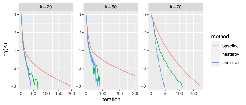
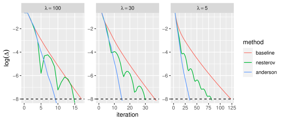
In this section we compare the proposed three methods, i.e. baseline, Nesterov and Anderson WLRMA, on a small simulation example. We generate the data as follows. First we draw $A\in\mathbb{R}^{n\times r}$ and $B\in\mathbb{R}^{p\times r}$ from standard normal distribution and compute $M=AB^{\top}+E.$ Here $E\in\mathbb{R}^{n\times p}$ is some matrix of errors drawn from $\mathcal{N}(0,\sigma^{2})$. We further generate the matrix of weights $W\in\mathbb{R}^{n\times p}$ via uniform distribution. In our experiments we set $n=1000$, $p=100$, $r=70$ and $\sigma=1.$ We initialize $X^{(0)}$ at zero matrix and using the three suggested algorithms, i.e baseline, Nesterov and Anderson WLRMA, we solve problems (6) and (7). For the latter approach, we set depth equal to three. For non-convex WLRA we test $k=20,50,70$. To make the results compatible, for the convex relaxation we search for $\lambda$ that results in approximately the same value of the unpenalized loss (see optimization problem (6)). Thus we vary $\lambda$ in the grid $\lambda=100,30,5.$ We track the relative change in the loss, i.e.

$$\Delta^{(i)}=\left|\frac{\ell(X^{(i+1)})-\ell(X^{(i)})}{\ell(X^{(i)})}\right|.$$ (17)

Here

$$\ell(X)=\|\sqrt{W}*(M-X)\|^{2}_{F}$$

for the WLRMA problem and

$$\ell(X)=\frac{1}{2}\|\sqrt{W}*(M-X)\|^{2}_{F}+\lambda\|X\|_{*}$$

for the convex relaxation. We stop the algorithm as soon as the relative difference is less than some threshold, i.e. $\Delta^{(i)}<\epsilon.$ In our experiments, the maximum number of iterations is limited to $300$ and the convergence threshold is set to $\epsilon=10^{-8}.$

The results are presented in Figure 1. According to our simulation experiments, both acceleration methods reach the convergence points faster than the baseline. Moreover, Anderson improves the convergence speed much more than Nesterov in the case of the convex relaxation. Note also that the convergence of accelerated methods for non-convex WLRA is more erratic comparing to the baseline.

(a) Solving the non-convex WLRMA problem with different ranks $k$.

(b) Solving the WLRMA convex relaxation problem with different penalty factors $\lambda$.

Figure 1: Simulation example. Relative objective change vs. iteration number plotted for baseline, Nesterov and Anderson $m=3$ algorithms. We match the rank and penalty factor of non-convex and convex problems so that top and bottom panels have similar value of the unpenalized objective.

5 Stabilizing Anderson acceleration coefficients

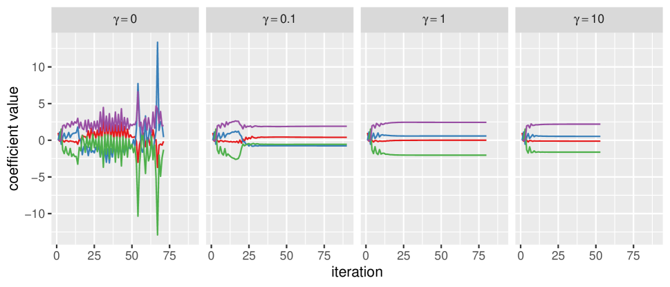
In this section we propose a way to stabilize the behavior of Anderson acceleration in the case of non-convex WLRMA. First, let us plot the coefficient paths, i.e. $\alpha$ vs. iteration. In the left panel of Figure 2 we present the paths produced while solving the WLRMA problem with $k=50$. We observe some significant oscillation in the coefficients, which results in the oscillation of the convergence path of Anderson WLRMA in Figure 1(a) (blue curve on the middle panel).

Figure 2: Coefficient paths obtained via Andersen acceleration with $m=3$ while solving the WLRMA problem for $k=50$. Each of the $m+1$ coefficients is represented in different color. Left panel corresponds to acceleration without stabilization (blue curve on the middle panel in Figure 1(a)). The remaining panels represent acceleration with different smoothing penalties $\gamma$ and $\alpha_{prev}$ equal to the average of three previous coefficient vectors.

To stabilize the coefficient paths we add regularization and restate problem (13) as

$$\operatornamewithlimits{minimize}_{\alpha=(\alpha_{m},\ldots,\alpha_{0})^{\top}}\|R^{(i)}\alpha\|_{2}^{2}+\gamma\|\alpha-\alpha_{prev}\|_{2}^{2}\quad\mbox{ subject to }\sum_{i=0}^{m}\alpha_{i}=1.$$ (18)

Here $\alpha_{prev}$ is the coefficient vector obtained on the previous iteration (regularization depth is equal to one), or the average of $d$ coefficient vectors obtained on several previous iterations (regularization depth is equal to $d$). The penalty in the above problem works in a similar way as acceleration methods: it balances the new update of the optimized variable with the previous guesses thereby smoothing the coefficient paths. On can derive the solution for problem (18).

$$\alpha^{*}_{\gamma}=(I+\gamma K)\alpha^{*}\mbox{ where } K=\big{(}R^{{(i)}^{\top}}R^{(i)}+\gamma I\big{)}^{-1}\big{(}\alpha_{prev}\textbf{1}^{\top}-\textbf{1}\alpha_{prev}^{\top}\big{)}$$

$$\alpha^{*}=\frac{\left(R^{{(i)}^{\top}}R^{(i)}+\gamma I\right)^{-1}\mathbf{1}}{\mathbf{1}^{\top}\left(R^{{(i)}^{\top}}R^{(i)}+\gamma I\right)^{-1}\mathbf{1}}$$

Note that computing $\alpha^{*}_{\gamma}$ involves some simple manipulations with the small $(m+1)\times(m+1)$ covariance matrix of the residuals $R^{(i)}$. Since this matrix is also required to be computed while deriving the unpenalized solution (14), the cost for regularized and non-regularized Anderson is equivalent.

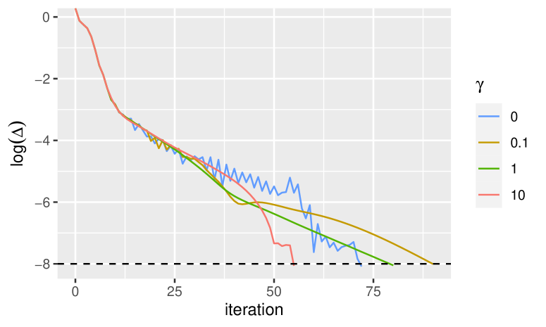
Now we test the proposed regularization technique on the same WLRMA problem. We vary $\gamma$, the smoothing penalty factor, in the grid $\gamma=0.1,1,10$ and consider the average of three previous coefficient vectors for $\alpha_{prev}$. The resulting coefficient paths are presented in Figure 2. As expected, increasing $\gamma$ smooths the coefficient paths. We compare the convergence speed for different $\gamma$ values. According to Figure 3 regularization also makes the convergence curves more smooth. Moreover, for large enough values of $\gamma$ stabilizing Anderson coefficients allows us to reach the convergence point faster.

Figure 3: Convergence comparison for Anderson ($\gamma=0$) and stabilized Anderson ($\gamma=0.1,1,10$). We set $\alpha_{prev}$ to the average of the previous three coefficient vectors. We solve the WLRMA problem for $k=50$, thus blue curve on this plot corresponds to the blue curve on the middle plot of Figure 1(a).

6 High dimensions

6.1 Alternating least squares

In some applications, where $n$ and/or $p$ are extremely large the SVD part of the proximal operator is not plausible. For example, in the Netflix competition the training data matrix was approximately $400K$ by $20K$. In this section we borrow an idea from Hastie et al. (2015), proposed for the low-rank matrix approximation problem with missing values, that allows us to avoid the SVD in high dimensions.

Similar to (4) it is possible to restate the WLRMA problem as

$$\operatornamewithlimits{minimize}_{A\in\mathbb{R}^{n\times k},B\in\mathbb{R}^{p\times k}}\|W*(M-AB^{\top})\|^{2}_{F}$$ (19)

This alternative view of the WLRMA problem is well-studied in literature (see, for example Razenshteyn et al., 2016; Dutta et al., 2018), where the authors propose simple iterative least squares algorithm that alternates two steps: fix $A$ and solve a weighted least squares problem to find $B$; then do the same for $A$ fixing $B$. Although the algorithm avoids the most expensive SVD part of the PGD computations, for general $W$, it is still only moderately efficient as multiple weighted regressions are required for each step (one for each row of $A$ and $B$).

It is easy to show that the proximal step for (6) is equivalent to solving (19) with $M=X-\nabla g(X)=Y$ and unit weights, i.e. $W=1_{n\times p}$. Thus the alternating least squares update can be done via solving an unweighted multiresponse regression problem. To be precise, we get the following updates for non-convex WLRMA

$$B=Y^{\top}A(A^{\top}A)^{-1}\mbox{ and }A=YB(B^{\top}B)^{-1},$$ (20)

which leads us to the following SVD-free alternating algorithm.

Algorithm 2 WLRMA-ALS

1. Initialize

   1. Set $A^{(0)}\in\mathbb{R}^{n\times k}$ and $B^{(0)}\in\mathbb{R}^{p\times k}$ at random.

2. Repeat until convergence

   1. Compute $X^{(i)}=A^{(i)}B^{{(i)}^{\top}}$ and $Y^{(i+1)}=W*M+(1-W)*X^{(i)}.$

   2. Set $B^{(i+1)}:=Y^{{(i+1)}^{\top}}A^{(i)}\big{(}A^{{(i)}^{\top}}A^{(i)}\big{)}^{-1}$

   3. Update $X^{(i)}=A^{(i)}B^{{(i+1)}^{\top}}$ and $Y^{(i+1)}=W*M+(1-W)*X^{(i)}.$

   4. Set $A^{(i+1)}:=Y^{{(i+1)}}B^{(i+1)}\big{(}B^{{(i+1)}^{\top}}B^{(i+1)}\big{)}^{-1}.$

Note that quite many variations of the above algorithm can be derived. For example, one can skip an extra update of $X^{(i)}$ and $Y^{(i+1)}$ (step 2.3). To recover the exact result of the projection step one should alternate 2.2 and 2.4 until the convergence.

It is not hard to build similar algorithm for the WLRMA convex relaxation. We first claim that for each $\lambda>0$ there exists $r$ such that for all $k>r$ problem (7) is equivalent to solving penalized problem

$$\operatornamewithlimits{minimize}_{A\in\mathbb{R}^{n\times k},B\in\mathbb{R}^{p\times k}}\frac{1}{2}\|W*(M-AB^{\top})\|^{2}_{F}+\frac{\lambda}{2}\|A\|^{2}_{F}+\frac{\lambda}{2}\|B\|_{F}^{2}$$ (21)

Next, note that if one matrix ($A$ or $B$) is fixed and the weights are unit, then the other matrix can be found via solving a ridge regression problem. Thus replacing the ALS updates at step 2.2 of the above algorithm by

$$B=Y^{\top}A(A^{\top}A+\lambda I)^{-1}\mbox{ and }A=YB(B^{\top}B+\lambda I)^{-1}$$ (22)

we get a simple alternating procedure solving the WLRMA convex relaxation (7).

To check the convergence of the algorithm one needs to compute the loss functions of (19) or (21). This, again, can be done efficiently using the sparse structure of $W$.

6.2 Sparse weights

In some applications the matrix of weights $W$ can be very sparse. For instance, in the Netflix application, where almost all movie ratings are unobserved, $W$ will mostly contain zeros. It turns out that for sparse weight matrices the storage and computational cost of the ALS algorithm can be significantly reduced. The trick we propose below is especially useful when the high dimensionality of the problem makes it impossible to store $n\times p$ matrices.

Denote $\Omega$ the set of non-zero element of $W$. Following Hastie et al. (2015) we first note that matrix $Y^{(i+1)}$ at step 2.1 and 2.3 can be represented in a sparse + low-rank form as follows:

$$Y^{(i+1)}=\underbrace{W*(M-X^{(i)})}_{sparse}~{}~{}~{}+\underbrace{X^{(i)}}_{low-rank}=S^{(i)}+X^{(i)}.$$

Here the second term $X^{(i)}$ is a high-dimensional but low-rank matrix, that can be stored in the form of $(A,B)$ pair. Furthermore, the first term $S^{(i)}$ is a sparse matrix, which takes only $O(k\times|\Omega|)$ to compute (using the low-rank structure of $X^{(i)}$) and which can be stored in the form of a $|\Omega|$-dimensional vector. This leads us to the implementation of ALS in algorithm 3.

Algorithm 3 WLRMA-ALS-sparse

1. Initialize

   1. Set $A^{(0)}\in\mathbb{R}^{n\times k}$ and $B^{(0)}\in\mathbb{R}^{p\times k}$ at random.

2. Repeat until convergence

   1. Compute sparse $S^{(i)}=W*(M-A^{(i)}B^{{(i)}^{\top}}).$

   2. Compute $H_{A}=A^{(i)}\big{(}A^{{(i)}^{\top}}A^{(i)}\big{)}^{-1}$ and set $B^{(i+1)}=B^{{(i)}^{\top}}A^{{(i)}}H_{A}+S^{{(i)}^{\top}}H_{A}.$

   3. Update sparse $S^{(i)}=W*(M-A^{(i)}B^{{(i+1)}^{\top}}).$

   4. Compute $H_{B}=B^{(i+1)}\big{(}B^{{(i+1)}^{\top}}B^{(i+1)}\big{)}^{-1}$ and set $A^{(i+1)}=A^{(i)}B^{{(i+1)}^{\top}}H_{B}+S^{{(i)}}H_{B}$

Note that $H_{A}$ and $H_{B}$ are cheap to calculate via multiplying skinny matrices. Moreover, step 2.2 and 2.4 can be simplified to

$B^{(i+1)}=B^{(i)}+S^{{(i)}^{\top}}H_{A}$ and $A^{(i+1)}=A^{(i)}+S^{(i)}H_{B}$,

respectively. Then steps 2.2. and 2.4 are easy to handle using the sparse structure of $S^{(i)}$, thereby making the computations for the ALS algorithm very efficient.

Finally, for the convex relaxation we can simply use

$H_{A}=A^{(i)}\big{(}A^{{(i)}^{\top}}A^{(i)}+\lambda I\big{)}^{-1}$ and $H_{B}=B^{(i+1)}\big{(}B^{{(i+1)}^{\top}}B^{(i+1)}+\lambda I\big{)}^{-1}$

which still reduces to “cheap” multiplication of skinny matrices and inverting a small $r\times r$ matrix.

6.3 Acceleration in high dimensions

It is possible to extend all the tricks proposed in Section 6 to accelerated methods as well. For both Nesterov and Anderson acceleration we exploit the following idea. Note that each iteration of the WLRMA-ALS (and its sparse modification) algorithm can be considered as an operator on a pair of matrices $(A,B)$. Specifically, at step 2.1 the algorithm takes $(A^{(i)},B^{(i)})$ and after some transformation at steps 2.1–2.4 it returns the updated pair $(A^{(i+1)},B^{(i+1)}).$ For simplicity, let us denote this operator by $\Phi(A,B)$; this operator will be the main building block of our acceleration algorithm. Further, to introduce acceleration to the algorithm we concatenate matrices $A$ and $B$ an denote the result by $Z$, thus $Z=\begin{pmatrix}A\\ B\end{pmatrix}$. To build our accelerated ALS approaches we apply acceleration to $Z$. For example, in the Nesterov case this will be equivalent to applying acceleration separately to $A$ and $B$.

Algorithm 4 WLRMA-ALS-Nesterov

1. Initialize

   1. Set $A^{(0)}\in\mathbb{R}^{n\times k}$ and $B^{(0)}\in\mathbb{R}^{p\times k}$ at random.

2. Repeat until convergence

   1. Update $V_{A}^{(i)}=A^{(i)}+\frac{i-1}{i+2}\left(A^{(i)}-A^{(i-1)}\right)$ and $V_{B}^{(i)}=B^{(i)}+\frac{i-1}{i+2}\left(B^{(i)}-B^{(i-1)}\right).$

   2. Update $\big{(}A^{(i+1)},B^{(i+1)}\big{)}:=\Phi\big{(}V_{A}^{(i)},V_{B}^{(i)}\big{)}$

To build Anderson acceleration we consider our baseline-ALS algorithm as a successive application of the update $Z^{(i+1)}=\Phi(Z^{(i)})$. This leads us to the fixed-point equation $Z=\Phi(Z)$, which can be solved via Anderson acceleration outline discussed in Section 3.2. Note that the resulting method will operate in terms of skinny $(n+m)\times k$ matrices which makes it very efficient in terms of both computational and storage cost.

6.4 Find the solution rank

Sometimes it can be useful to track the solution rank while updating $A$ and $B$. For example, one can consider the delayed Anderson acceleration (see Section 3.2) and initialize the acceleration as soon as the solution rank becomes less than $k$. To calculate the solution rank for low-rank $X=AB^{\top}$ one can apply the following simple steps:

• Decompose $A$, i.e. $A=U_{A}D_{A}V_{A}^{\top}$.

• Multiply $\tilde{B}=BV_{A}D_{A}$.

• Decompose $\tilde{B}=U_{B}D_{B}V_{B}^{\top}$.

Thus $X=(U_{A}V_{B})D_{B}U_{B}^{\top}$ is the SVD of $X$ and the number of non-zero elements in $D_{B}$ will represent the solution rank. Again, since we work in terms of skinny matrices only, the SVD is cheap to compute.

7 MovieLens data

In this section we test the proposed methods on a real dataset. The dataset describes a 5-star rating and from MovieLens, a movie recommendation service. It contains 1 million ratings from 6000 users on 4000 movies that we store in a large $6000\times 4000$ matrix $M$. Note that $M$ is very sparse: some of the movies were rated by just a few users (if any) and only 5% of values are observed. Although the SVD-based approaches proposed in Sections 2–3 could be applied to this data, each iteration takes several minutes to complete, which makes the convergence process extremely slow.

In Figure 4 we present the results for three ALS methods: baseline, Nesterov and Anderson with depth $m=3$. To initialize the algorithms we use a warm start, which is the ALS solution for non-weighted problem with unobserved values of $X$ replaced by zeroes. To guarantee that loss decreases at each iteration for Anderson Acceleration we use the guarded modification (see Section 3.2). Using the three algorithms under consideration we solve the WLRMA convex relaxation problem varying $\lambda$ in the grid $\lambda=40,50,100$ which results in the solutions of rank $70,20$ and $5$, respectively. We limit the maximum number of iterations to $200$ and set the convergence threshold to $\epsilon=10^{-8}.$

Figure 4: MovieLens example. Comparison of three ALS algorithms: baseline, Nesterov and Anderson with $m=3$. The convex relaxation with different $\lambda$ is solved. Top panel represents the objective relative change vs. time. Bottom panel represents the solution rank vs. time.

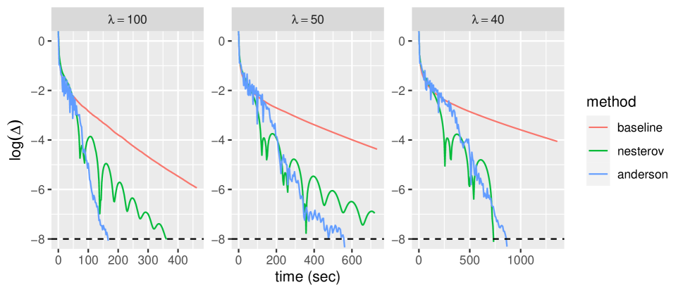
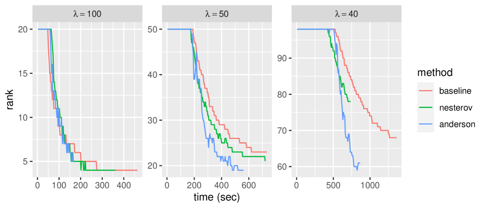
According to the Figure, all three methods achieve reasonable accuracy of $\epsilon=10^{-4}$ in just a few minutes. However, both acceleration methods demonstrate better convergence speed comparing to the baseline ALS technique. Note that for $\lambda=100,50$ Anderson achieves the threshold $\epsilon=10^{-8}$ much faster than the Nesterov. Although for $\lambda=40$ Nesterov is slightly faster than the competitor the rank plot (green curve on the bottom right panel) suggests that it stopped too early. Finally, we observe that for less accurate solutions, e.g. the ones with $\epsilon=10^{-4}$, Nesterov acceleration could outperform the Anderson approach.

8 Discussion

In this paper we proposed a weighted generalization of the low-rank matrix approximation technique. Both classical LRMA problem, which has an explicit solution, and the famous LRMA problem with missing values, which can be solved via iterative soft- or hard-impute algorithms, are special cases of this weighted generalization. To build the baseline algorithm solving the weighted problem we utilize proximal gradient descent. We further suggest two ways to accelerate the baseline method. The first technique is based on the Nesterov acceleration which uses the momentum from the previous iteration. To develop the second acceleration method we restate the WLRMA problem as a fixed-point equation and subsequently utilize Anderson acceleration.

There is still much scope for future work. One interesting direction is to test the proposed methods on some real-data applications with sparse but non-binary weights. For example, one can consider a GLM model with a working response having some low-rank matrix structure. Then each step of the Newton gradient descent will be equivalent to solving a weighted low-rank matrix approximation problem. Furthermore, if a huge portion of data is missing, it becomes a WLRMA problem with a sparse weight matrix. Another direction could be to explore the ways to improve the stability of the Anderson acceleration. There are many tricks beyond the ones discussed in this paper that could help us with this goal; for example, we can test Powell regularization or restart checking proposed in Zhang et al. (2020).

9 Software

Proposed methods are implemented in the R package WLRMA; the software is available from Github (https://github.com/ElenaTuzhilina/WLRMA).

10 Funding

Elena Tuzhilina was supported by Stanford Data Science Scholarship. Trevor Hastie was partially supported by grants DMS-2013736 And IIS 1837931 from the National Science Foundation, and grant 5R01 EB 001988-21 from the National Institutes of Health.

References

- (1)
- Anderson (1965) Anderson, D. G. (1965), ‘Iterative procedures for nonlinear integral equations’, J. ACM 12(4), 547–560.
- Ban et al. (2019) Ban, F., Woodruff, D. & Zhang, R. (2019), Regularized weighted low rank approximation, in ‘Advances in Neural Information Processing Systems’, Vol. 32, Curran Associates, Inc.
- Candes & Tao (2010) Candes, E. J. & Tao, T. (2010), ‘The power of convex relaxation: Near-optimal matrix completion’, IEEE Transactions on Information Theory 56(5), 2053–2080.
- Candès & Recht (2008) Candès, E. & Recht, B. (2008), ‘Exact matrix completion via convex optimization’, 9, 717–772.
- Combettes & Pesquet (2011) Combettes, P. L. & Pesquet, J.-C. (2011), Proximal Splitting Methods in Signal Processing, Springer New York, pp. 185–212.
- Combettes & Wajs (2005) Combettes, P. L. & Wajs, V. R. (2005), ‘Signal recovery by proximal forward-backward splitting’, Multiscale Modeling & Simulation 4(4), 1168–1200.
- Dutta et al. (2018) Dutta, A., Li, X. & Richtárik, P. (2018), ‘Weighted low-rank approximation of matrices and background modeling’, CoRR .
- Dutta et al. (2021) Dutta, A., Liang, J. & Li, X. (2021), ‘A fast and adaptive svd-free algorithm for general weighted low-rank recovery’.
- Eckart & Young (1936) Eckart, C. & Young, G. (1936), ‘The approximation of one matrix by another of lower rank’, Psychometrika 1(3), 211–218.
- Feuerverger et al. (2012) Feuerverger, A., He, Y. & Khatri, S. (2012), ‘Statistical Significance of the Netflix Challenge’, Statistical Science 27(2), 202 – 231.
- Hastie et al. (2015) Hastie, T., Mazumder, R., Lee, J. D. & Zadeh, R. (2015), ‘Matrix completion and low-rank svd via fast alternating least squares’, Journal of Machine Learning Research 16(104), 3367–3402.
- Mai & Johansson (2020) Mai, V. V. & Johansson, M. (2020), ‘Anderson acceleration of proximal gradient methods’.
- Mardia et al. (1979) Mardia, K., Kent, J. & Bibby, J. (1979), Multivariate analysis, Probability and mathematical statistics, Acad. Press.
- Markovsky (2011) Markovsky, I. (2011), Low Rank Approximation: Algorithms, Implementation, Applications, Springer Publishing Company, Incorporated.
- Mazumder et al. (2010) Mazumder, R., Hastie, T. & Tibshirani, R. (2010), ‘Spectral regularization algorithms for learning large incomplete matrices’, Journal of Machine Learning Research 11(80), 2287–2322.
- Nesterov (1983) Nesterov, Y. (1983), ‘A method for solving the convex programming problem with convergence rate ’, Proceedings of the USSR Academy of Sciences 269, 543–547.
- Nguyen et al. (2019) Nguyen, L. T., Kim, J. & Shim, B. (2019), ‘Low-rank matrix completion: A contemporary survey’, IEEE Access 7, 94215–94237.
- Razenshteyn et al. (2016) Razenshteyn, I., Song, Z. & Woodruff, D. P. (2016), Weighted low rank approximations with provable guarantees, STOC ’16, Association for Computing Machinery, New York, NY, USA, p. 250–263.
- Rennie & Srebro (2005) Rennie, J. & Srebro, N. (2005), Fast maximum margin matrix factorization for collaborative prediction, pp. 713–719.
- Robin et al. (2019) Robin, G., Josse, J., Éric Moulines & Sardy, S. (2019), ‘Low-rank model with covariates for count data with missing values’, Journal of Multivariate Analysis 173, 416–434.
- Srebro & Jaakkola (2003) Srebro, N. & Jaakkola, T. (2003), Weighted low-rank approximations, in ‘Proceedings of the Twentieth International Conference on International Conference on Machine Learning’, ICML’03, AAAI Press, p. 720–727.
- Tuzhilina et al. (2020) Tuzhilina, E., Hastie, T. J. & Segal, M. R. (2020), ‘Principal curve approaches for inferring 3D chromatin architecture’, Biostatistics .
- Walker & Ni (2011) Walker, H. F. & Ni, P. (2011), ‘Anderson acceleration for fixed-point iterations’, SIAM Journal on Numerical Analysis 49(4), 1715–1735.
- Zhang et al. (2020) Zhang, J., O’Donoghue, B. & Boyd, S. (2020), ‘Globally convergent type-i anderson acceleration for nonsmooth fixed-point iterations’, SIAM Journal on Optimization 30(4), 3170–3197.
- Łukasz Kidziński et al. (2020) Łukasz Kidziński, Hui, F. K. C., Warton, D. I. & Hastie, T. (2020), ‘Generalized matrix factorization’.