[] Overinference from Weak Signals and Underinference from Strong Signals

1 Introduction

People face a constant stream of new information about future events. For example, people might read a new poll about a politician’s favorability, have a brief conversation with their boss at work, or see news about daily stock-market movements. Much of this information is only weakly informative about the relevant future events — whether the politician will be reelected, whether the person will be promoted, or whether they will have enough money for retirement. How do people update their beliefs in response to these types of weakly informative signals? While there is a large literature studying belief updating, it primarily focuses on people’s reactions to information that is relatively strong, with the common finding that people tend to underinfer from such information. We use new experimental and empirical evidence to show that, while people do underinfer from strong pieces of information, they overinfer from weak pieces of information — behavior that is consistent with a simple theory of cognitive imprecision. Consistent overinference from weak signals leads individuals to overvalue low-quality news, and to form beliefs that are overly extreme and excessively volatile.

We start with the observation that weak-signal settings are understudied in the experimental literature. The online appendix of [11]’s (B19) survey of the literature, for example, lists over 500 experimental treatment blocks across 21 papers that study inference from symmetric binary signals about a binary state. In none of these papers do subjects see signals that have a diagnosticity — the likelihood of seeing an “high” signal conditional on the “high” state — lower than $3/5$. Belief updating in these settings often features underreaction to new information relative to the Bayesian benchmark, particularly when signals are very strong, and much of the past literature has settled on underinference as the dominant form of probabilistic reasoning. For example, [11]’s (B19) “Stylized Fact 1” states that “Underinference is by far the dominant direction of bias.” Given the limited space of signals studied, however, the experimental literature has had little to say about the reaction to signals with lower diagnosticity.

Identifying updating errors outside of the laboratory is more challenging because both people’s beliefs and the correct Bayesian beliefs are often unobservable. One prominent strand of such work uses asset prices as proxies for beliefs or expectations. For individual stocks, there is robust evidence of predictable post-earnings announcement drift — in which a firm’s stock price tends to continue drifting in the same direction as the initial change after an earnings announcement — which appears consistent with initial underreaction to the announcement. But this finding seems to conflict with the large literature on excess volatility in overall stock-market valuations, which instead appears consistent with overreaction. While there are many candidate explanations seeking to reconcile these findings, we focus specifically on the role of signal informativeness. Pieces of news like company earnings announcements are relatively informative ([68]), while much of the information that drives daily market price changes (and volatility) is only weakly informative.

Our core goal, then, is to study how reaction to information varies when signals are weak versus strong. To do so, we both create (in the lab) and find (in asset-price data) environments in which signal strengths vary systematically and updating behavior can be measured consistently.

This is relatively straightforward in an experimental setting, where we have full control of the data-generating process (DGP): in the main treatment of our pre-registered experiment, we study a simple updating environment and vary the signal strength more comprehensively than has been done in past work. In particular, in the simplest treatment block, we expose 500 people to 16 different signal strengths in a version of a commonly used “bookbag-and-poker-chips” experimental design (e.g. [60]) in which people receive one binary signal about a binary state.

The main result of our experiment is that, while people underinfer from strong signals, they overinfer from weak signals. In the simple treatment block, subjects have a prior of $\pi_{0}=1/2$ about a binary state and receive a binary signal with diagnosticity $p>1/2$ that would move a Bayesian to a posterior of $\pi_{1}=p$ that the more likely state will occur. Consistent with nearly all existing evidence, for strong signals for which $p\geq 2/3$, we find robust evidence for underinference: subjects form posteriors $\hat{\pi}_{1}$ that are significantly below $p$. For $p\in[3/5,2/3]$, we do not find clear evidence for over- or underinference: the difference between $\hat{\pi}_{1}$ and $p$ is small. However, for $p\in(1/2,3/5)$, we find clear and robust evidence for overinference: $\hat{\pi}_{1}$ is statistically significantly greater than $p$, and the effect is convex in $p$. For very weak signals, subjects act as if signals are twice as strong as they truly are.

The shape of the belief response function maps closely to the predictions of a theory of cognitive imprecision that we extend, adapting ideas from psychophysics into economic decisionmaking ([29]; [45]). Specifically, we use a meta-Bayesian model in which people are cognitively imprecise about the signal strength $\mathbb{S}$ (similar to models in [59] and [71]). As a consequence, people’s average perception of signal strength — $\hat{\mathbb{S}}=k\cdot\mathbb{S}^{\beta}$ for $\beta\in(0,1)$ — is biased towards “intermediate” strengths. This leads them to perceive weak signals as stronger than they are and strong signals as weaker than they are. In our data, we estimate that $\beta=0.76$ and $k=0.88$, and that there is a switching point of $p=0.64$ at which people switch from overinference to underinference. Given this estimate, it is unsurprising that the plethora of experiments which use signals of precision greater than 0.64 find underinference.

While our simple model’s predictions might plausibly arise from a range of potential psychological microfoundations, we do find further evidence in line with our framework when exploring heterogeneity in treatment effects. Consistent with cognitive naivete affecting misinference, subjects with lower scores on a cognitive reflection test (a modified version of the classic test in [30]) both infer more from weak signals and infer less from strong signals. Relatedly, naivete within the experiment is related to more severe biases; using a within-subject test, we find that subjects who have had more experience in the experiment misinfer less in both directions. Finally, consistent with imprecision being an explanatory factor, we find that subjects with higher variance in how they perceive signals misinfer more in both directions. These heterogeneities suggest that cognitive imprecision affects both the overinference and underinference biases in belief updating, expanding upon the work by [71] and [27] in different decision problems.

If people systematically overinfer from weak signals and underinfer from strong signals, they may overvalue low-quality news and undervalue high-quality news, patterns that are borne out in our data. In an additional treatment of the experiment, subjects are asked to purchase up to three signals of varying strengths. Compared to a payoff-maximizing benchmark, subjects purchase too many weak signals and too few strong signals. These effects can be explained by misinference from both signal strength and signal quantity. To test the latter, we run an additional treatment that varies the number of signals subjects receive, finding consistent evidence that subjects underreact to the quantity of signals (as previously documented by [39]; [13]; and [12]). Combining these factors, people particularly overvalue observing individual weak signals and undervalue observing multiple strong signals.

We use other experimental treatments to explore mechanisms behind these findings. We show that our main results are driven by distorting signal processing, not by distorting probabilities (unlike, for instance, [43]; [66]; and [27]). We are able to distinguish between signal processing distortions and probability distortions by considering how subjects infer from asymmetric signals. A signal that happens to have a likelihood of close to 0.5 does not systematically affect inference, suggesting that it is the signal that is misperceived as opposed to its associated probability. Additionally, we show that, when faced with signals of an uncertain strength, results suggest that people act as if they misperceive possible realizations of the signal.

While our experiment allows us to cleanly identify over- and underinference, there are reasons to think that the behavior we observe may not carry over to real-world situations. First, rewards for accuracy in an experiment are relatively small, so one might think that people will work to correct their biases in higher-stakes environments (e.g. [50]). Second, the setting of the experiment is abstract and unfamiliar to subjects, so they may rely more on heuristics; in real-world settings with more sophisticated people, perhaps familiarity and experience will drive beliefs towards true probabilities (e.g. [52]).

In light of these concerns, we next turn to evidence from more realistic high-stakes settings by studying the movement of market-implied probability distributions in betting and financial markets. A key challenge with testing any theory of updating in real-world observational data is that we no longer have direct knowledge of the true DGP or signal strength. To overcome this challenge, we develop a new empirical method based on theoretical results from [5] and [4]. The core intuition of these papers is that, when a Bayesian is changing their beliefs over time about some event, they must be learning something and therefore (on average) must reduce their uncertainty correspondingly. This intuition can be formalized by defining movement as the sum of the squared deviations of changes in beliefs over time, and uncertainty reduction as the drop in perceived variance in the outcome. While movement and uncertainty reduction may differ for a given signal realization, they must be equal in expectation across signal realizations, regardless of the DGP. This insight allows for a DGP-agnostic test of Bayesian updating in observational data. And crucially for our analysis, these statistics are intuitively and theoretically related to over- and underreaction: overreaction will lead to positive excess movement (movement greater than uncertainty reduction) on average, while underreaction will lead to too little movement relative to the reduction in uncertainty.

While this allows for an intuitive test of over- vs. underreaction with an unknown DGP, to test our theory, we also need to distinguish situations in which signals are weak versus strong. Given that the signal strength is also unobservable, we must instead turn to an ex-ante known (and observable) separating variable that is related to signal strength. Our innovation here is to focus on time to resolution as our separating variable. Intuitively, when a person is predicting the value of the S&P 500 in three months, information today should generally not lead to much belief movement; meanwhile, information today is highly informative for the value of the S&P tomorrow, and we should accordingly observe more movement of short-horizon beliefs in response to information.

Our theory then intuitively suggests that there should be overreaction (and too much movement) at long forecast horizons, and underreaction (and too little movement) at short horizons. We first confirm, by simulating simple DGPs matching our empirical setting, that this pattern exists for an agent who misperceives according to our theory, and that this pattern differs from that under Bayesian updating or constant under- or overreaction. We then turn to the data. We first study sports-betting data, making use of over 5 million transactions from a large sports prediction market for five major sports (corresponding to more than 20,000 sporting events). We then study S&P 500 index option markets, using option-implied beliefs regarding the future value of the S&P from over 4 million daily option prices (corresponding to 5,500 trading dates and 955 option expiration dates).

We start by plotting the average movement and uncertainty reduction over time for the sports and financial data. Both uncertainty reduction and movement are generally increasing as the event continues and resolution approaches. However, movement is generally higher than uncertainty reduction at the beginning of the event and lower at the end of the event. For example, in the options data, there is very little daily uncertainty reduction until a few weeks before the contract expires, but beliefs consistently move back and forth, generating positive movement. In other words, news today appears to hold relatively little information about the value of the S&P in multiple months, but the market acts as if has more diagnosticity. However, within two weeks of a contract’s resolution, the relationship reverses: movement is either less than or equal to uncertainty reduction. That is, as signals become stronger, the market begins to underreact. On net, total movement averaged over an entire option contract is too high, matching the finding of excess movement in [4]. But this overall average masks meaningful heterogeneity as one varies the signal strength, with markets misperceiving in the manner predicted by our theory. The same broad pattern holds in the sports-betting data we consider.

To statistically test this relationship, we regress average movement on average uncertainty reduction in a given time window (where time is measured as distance to resolution). While a Bayesian should have a constant of 0 and slope of 1 in such a regression, we show that the constant is significantly positive and the slope is significantly less than one. The positive constant indicates that when signals are likely to be weak (uncertainty reduction is low), there is too much belief movement. The less than one-for-one slope indicates that as signals become stronger (uncertainty reduction increases), there is a point at which the relationship flips, and there is too little belief movement.

Given that we cannot observe true signal strength, we must rely on our indirect measure (time to resolution) to test the relationship between signal strength and over- vs. underreaction in real-world high-stakes settings. The strength of our experimental setting, meanwhile, is that these variables are fully observable, but the experiment is lower-stakes and less realistic. The two settings thus provide complementary evidence for our theory, whose predictions align well with both sets of data.

Our main experimental results relate to numerous papers on the topic of belief updating, including several papers that present evidence for other forms of over- and underreaction to information. Classically, [39] show that subjects underreact to the credence of a signal relative to its strength, and [56] show that subjects overreact to what a signal says relative to the environment that produces it. More recently, [35] find underreaction to strong signals but even further underreaction to the retraction of those signals, while [46] find overreaction to disconfirming signals, and [15] find overreaction to the retraction of certain types of information that may be classified as weak. This paper also relates to the use of cognitive imprecision in inference problems, such as in [27] and [65], that finds relationships between underreaction to strong pieces of evidence and cognitive imprecision. There is evidence that other forms of decision problems may induce overreaction, as shown by [28] and [1], so we focus on this particular decision problem.

More recently, [7] run an experiment that confirms many of the patterns that we originally documented in our experiment: they also vary signal diagnosticity and find overreaction to weak signals and underreaction to strong signals. Using theory and other treatments, they extend our findings to argue that individuals reduce the complexity of information structures before misinterpreting these structures in ways consistent with cognitive imprecision. By contrast, they do not analyze non-experimental data, whereas we provide additional empirical evidence from sports-betting and financial markets. We see these papers as highly complementary.

Our results are thus further related to a large literature on asset prices and beliefs, as surveyed recently in [9]. [14] provide an early discussion of the possible link between post-earnings drift and underreaction, while [24] do so for the connection between excess volatility and overreaction. [48] aim to reconcile these findings through the lens of the extremeness (or fat-tailedness) of the true distribution of outcomes. We focus instead on the informativeness of signals about a given outcome, which is conceptually different from the extremeness of the outcome distribution.

The paper proceeds as follows. Section 2 introduces the theoretical framework; Section 3 details the experimental design; Section 4 presents the experimental results; Section 5 analyzes the market data; and Section 6 discusses our results and concludes. The Appendix contains additional results and empirical details, and screenshots of the pages in the experiment are provided in the Supplementary Appendix.

2 Theory

2.1 Setup and Intuition

We consider individuals who may misinterpret information they receive. In the environment we study, people begin with a prior at time 0, then receive a signal $s$ about a binary state $\theta\in\{0,1\}$, and form a posterior at time 1. An individual has a prior $\pi_{0}\equiv P(\theta=1)$. The signal either sends a low message or a high message ($s_{L}$ or $s_{H}$), with $P(\theta=1|s_{H})>P(\theta=1|s_{L})$. After seeing signal $s$, the individual forms a posterior belief $\pi_{1}(s)\equiv P(\theta=1|s)$, which we typically shorten to $\pi_{1}$. Defining the logit function $\text{logit}(\pi)\equiv\log\left(\frac{\pi}{1-\pi}\right)$, a Bayesian would form a posterior such that $\text{logit}(\pi_{1})=\text{logit}(\pi_{0})+\log\left(\frac{P(s|\theta=1)}{P(s|\theta=0)}\right)$ (using the setup developed in [37]). We consider a misperceiving person who may over- or underinfer from information and instead forms a posterior of $\text{logit}(\hat{\pi}_{1})=\text{logit}(\pi_{0})+w\log\left(\frac{P(s|\theta=1)}{P(s|\theta=0)}\right)$.

Misperception of Signal Strength

The strength of a signal is defined by its log odds ratio: $\mathbb{S}\equiv\left\lvert\log\left(\frac{P(s|\theta=1)}{P(s|\theta=0)}\right)\right\rvert\in[0,\infty)$. We study how $w$ depends on $s$ through $\mathbb{S}$. We posit that when people receive a signal of strength $\mathbb{S}$, they systematically distort their perception of its strength when using it to form posterior $\hat{\pi}_{1}$. Following [59], and [71], individuals in our model misperceive $\mathbb{S}$ via a form of cognitive imprecision. First, as described by the classic Weber-Fechner law, they interpret changes in $\mathbb{S}$ in relative terms instead of in absolute terms ([29]). Second, they are uncertain as to what the true signal strength is.

Specifically, we follow [71] in assuming that a misperceiving person represents signal strengths $\mathbb{S}$ with a value $r$, which is drawn from a normal distribution with imprecision parameter $\eta$: $r\sim\mathcal{N}(\log\mathbb{S},\eta^{2})$. They have a “cognitive prior” about how strong signals tend to be, and this belief is distributed log-normally: $\log\mathbb{S}\sim\mathcal{N}(\mu_{0},\sigma^{2})$. They update using Bayes’ rule when observing a signal; given $r$, their perceived posterior expectation of $\mathbb{S}$ is

$$\hat{\mathbb{S}}(r)=\mathbb{E}[\mathbb{S}|r]=\exp\left[\left(\frac{\eta^{2}}{\sigma^{2}+\eta^{2}}\right)\log\bar{\mathbb{S}}+\left(\frac{\sigma^{2}}{\sigma^{2}+\eta^{2}}\right)r\right],$$

where $\bar{\mathbb{S}}\equiv\exp(\mu_{0}+\sigma^{2}/2)$ is the prior mean over signal strengths.

Therefore, their perception $\hat{\mathbb{S}}$ of the true signal strength $\mathbb{S}$ is distributed log-normally with mean equal to

$$\mathbb{E}[\hat{\mathbb{S}}]=k\cdot\mathbb{S}^{\beta},$$ (1)

where $k\equiv\exp(\beta^{2}\eta^{2}/2)\cdot\bar{\mathbb{S}}^{1-\beta}$ and $\beta\equiv\sigma^{2}/(\sigma^{2}+\eta^{2})\in(0,1)$.

Our main object of interest is the average level of over- and underinference for different values of $\mathbb{S}$, so we assume for now that each person perceives $\mathbb{S}$ to be exactly the expectation given by (1); that is, when they see a signal of strength $\mathbb{S}$, they always perceive it to be of strength $k\cdot\mathbb{S}^{\beta}$. This simplification makes the functional form a version of the classical one from [63], and it makes the analysis more tractable without affecting the main results qualitatively.

The misperception implied by Equation 1 can be described as the individual misweighting signals: by treating signal $\mathbb{S}$ as having strength $k\cdot\mathbb{S}^{\beta}=k\cdot\mathbb{S}^{-(1-\beta)}\cdot\mathbb{S}$, they are effectively weighting a signal with strength $\mathbb{S}$ by a factor of $k\cdot\mathbb{S}^{-(1-\beta)}$. There is a switching point $\mathbb{S}^{*}\equiv k^{\frac{1}{1-\beta}}$ for which this weight is below 1 (leading to overreaction) if $\mathbb{S}<\mathbb{S}^{*}$, and above 1 (leading to underreaction) if $\mathbb{S}>\mathbb{S}^{*}$.

Updating Given Symmetric Signals

We now focus on symmetric signal structures, which we use in the experiment, in which each signal has the same precision $p\equiv P(s_{H}|\theta=1)=P(s_{L}|\theta=0)>1/2$, and therefore the strength of each signal is $\mathbb{S}=|\text{logit}(p)|$. When the prior is $\pi_{0}=1/2$ (as in our experiment), then the Bayesian posterior equals the signal precision $\pi_{1}=p$. This leads to simplified formulas, which allows for a set of simple two-dimensional graphs that represent the core relationships in the model (we will reproduce these same graphs using experimental data in the next section).

While the Bayesian perceives signals as having the correct strength $\mathbb{S}$, the misperceiving person instead treats each signal as having a mean strength of

$$\hat{\mathbb{S}}=k\cdot(\text{logit}(p))^{-(1-\beta)}.$$ (2)

The top panel of Figure 1 plots the relationship between perceived and true strength (given the parameters $k$ and $\beta$ we estimate from the experiment). For comparison, we also plot the relationship for a Bayesian (for which they are equal) and a person who exhibits constant conservativism (for which perceived strength is always lower than reality). The misperceiving person in our model overreacts to weak signals, but underreacts to strong signals.

When a Bayesian observes a symmetric signal, they will update to either $p$ or $1-p$. Instead, the misperceiving person will update to either $\hat{p}$ or $1-\hat{p}$ at the mean perceived signal strength, where

$$\hat{p}=\frac{\exp(k\cdot(\text{logit}(p))^{\beta})}{1+\exp(k\cdot(\text{logit}(p))^{\beta})}.$$ (3)

That is, $\hat{p}$ can be seen as the perceived precision of the signal. The middle panel of Figure 1 plots the mapping between the perceived and true precision, which is another way of capturing the core error. The misperceiving person believes that signals with little precision are more precise than reality, and signals with high precision are less precise. Note that, as signals become arbitrarily informative or uninformative, their weighting function becomes arbitrarily small or large, but their posteriors converge to the Bayesian’s.

Following the discussion above, a final interpretation is that the individual is misweighting signals. Defining $\hat{w}(p)$ as the weighting function given precision $p$ yields

$$\hat{w}(p)\equiv k\cdot(\text{logit}(p))^{-(1-\beta)}.$$ (4)

The bottom panel of Figure 1 plots the weighting function relative to the precision $p$, again given our experimental parameters. The misperceiving person places too much weight on weak signals and too little weight on strong signals. This is the core prediction from our theoretical framework. While mechanisms other than cognitive uncertainty might generate qualitatively similar patterns, the particular power form of our predicted weighting function aligns closely with our experimental data, as discussed further below.

Figure 1: Theoretical Predictions of Over- and Underinference by Signal Strength

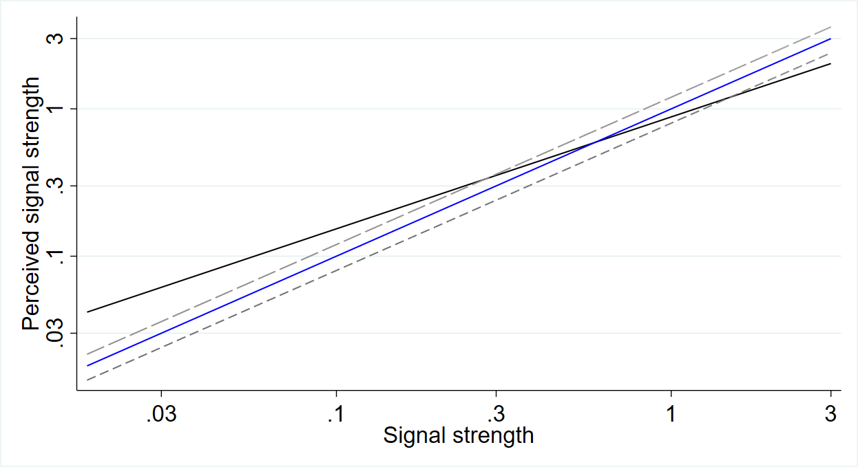
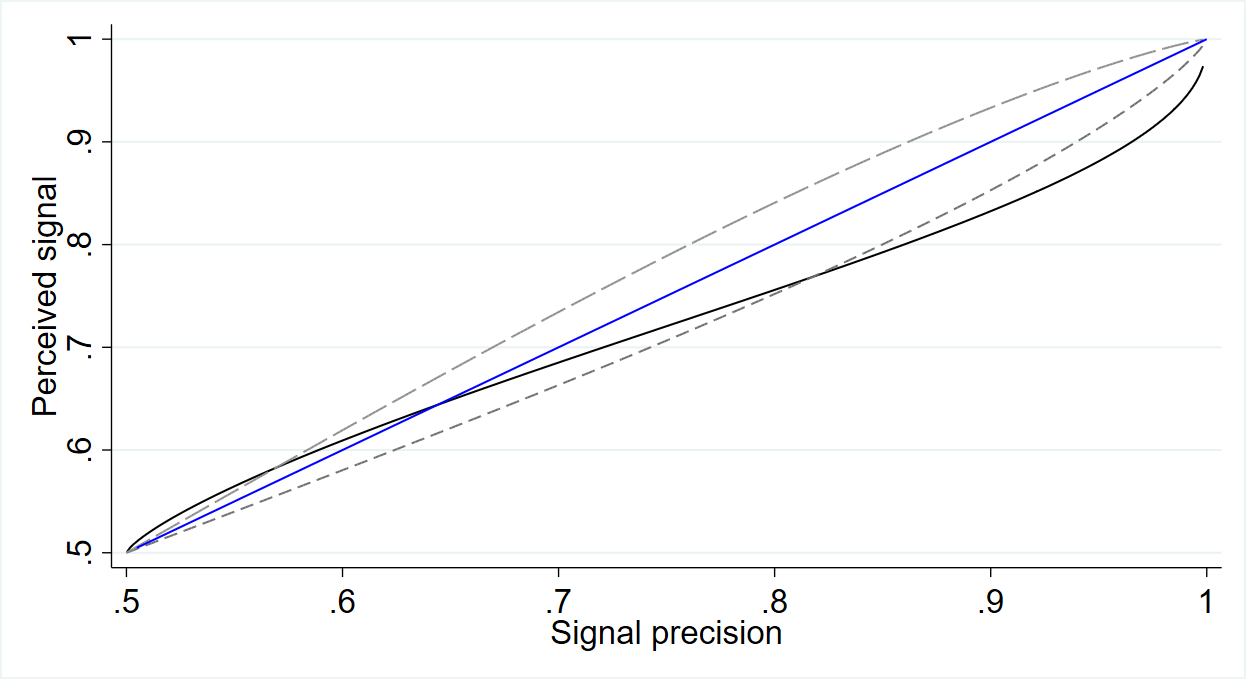
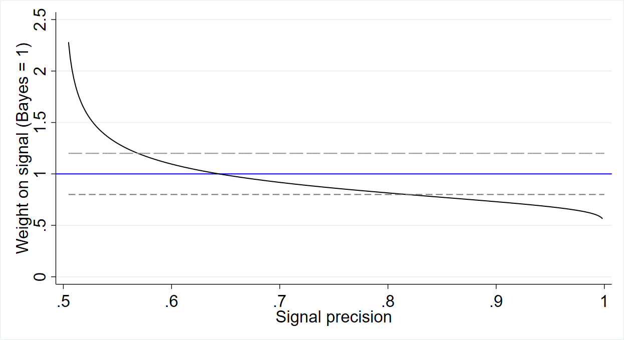
• Notes: These figures provide three representations of the core deviation in our model. Blue lines correspond to Bayesian updating (correct perception of signal strength $\mathbb{S}$), short dashed lines to underinference (with perceived signal strength $0.8\cdot\mathbb{S}$), long dashed lines to overinference (perceived signal strength $1.2\cdot\mathbb{S}$) and black lines to the misperception in our model (perceived signal strength $k\cdot\mathbb{S}^{\beta}$ with $k=0.882$ and $\beta=0.760$). The top panel plots signal strength perception as a function of signal strength on a log-log scale. The middle panel plots the perceived precision as a function of the true precision. The bottom panel plots the weight put on signals as a function of the true precision. All figures show that misperceiving individuals overweight weak signals and underweight strong signals.

2.2 General Model Predictions

Figure 1 shows some properties of the weighting function — in particular, how the agent switches from overinference to underinference as signal strength increases — for one particular parameter set. Proposition 1 shows that this is in fact a general property.

Proposition 1 (Misweighting Information).

The weighting function $\hat{w}(p)$ from Equation 4 and the precision $\hat{p}$ from Equation 3 have the following properties:

1. $\hat{w}(p)$ is decreasing in $p$.

2. There exists a switching point $p^{*}\equiv\frac{k^{\frac{1}{1-\beta}}}{1+k^{\frac{1}{1-\beta}}}$ such that:

   • If the Bayesian perceives the precision to be $p<p^{*}$, $\hat{p}>p$ and $\hat{w}(p)>1$.

   • If the Bayesian perceives the precision to be $p>p^{*}$, $\hat{p}<p$ and $\hat{w}(p)<1$.

The model also makes predictions about which types of individuals and situations will lead to greater overinference from weak signals and underinference from strong signals. Individuals with greater cognitive imprecision, as measured by $\eta^{2}$, act in a way that is further from Bayesian updating for both strong and weak signals. In particular, there is a value

$$\mathbb{S}^{\dagger}=\exp\left(\frac{\sigma^{2}(\sigma^{2}-\eta^{2})}{2(\eta^{2}+\sigma^{2})}\right)\text{ and }p^{\dagger}=\frac{\exp(\mathbb{S}^{\dagger})}{1+\exp(\mathbb{S}^{\dagger})},$$

at which $\frac{\partial\hat{w}(p)}{\partial\eta}>0$ iff $p<p^{\dagger}$. That is, cognitively precise people will behave similar to a Bayesian, while cognitively imprecise people will both overweight sufficiently weak signals and underweight sufficiently strong signals.

The misperceiving person’s instrumental value for a signal tracks signal perceptions. Suppose that after receiving the signal, the person is asked to take an action $a$, and they receive utility $1-(1-a)^{2}$ if $\theta=1$ and $1-a^{2}$ if $\theta=0$. In this setup, a person maximizes expected utility by taking the action corresponding to their belief. Given this choice, a person with belief $\hat{p}$ will expect to earn utility $\hat{p}(1-(1-\hat{p})^{2})+(1-\hat{p})(1-\hat{p}^{2})=1-\hat{p}(1-\hat{p})$. An individual who is aware that they will perceive a signal using Equation 3 will therefore instrumentally value a signal that moves beliefs from 1/2 to $\hat{p}$ at $1/4-\hat{p}(1-\hat{p})$. When individuals start with a prior of 1/2, this means that overinference will lead to excess demand for information and underinference will lead to too little demand, and there will be a switching point at $p^{*}$.

3 Experiment Design

This section overviews the design and the sample, then outlines the timing and treatment blocks, and lastly discusses further details of each treatment block. For full details on the experimental design, Supplementary Appendix C contains screenshots of each type of page.

3.1 Overview and Data

Subjects were told that a computer has randomly selected one of two decks of cards — a Green deck or a Purple deck — and both decks are equally likely ex ante. Each deck has Diamond cards and Spade cards: the Green deck has $D_{1}$ Diamonds and $N-D_{1}$ Spades, and the Purple deck has $D_{2}$ Diamonds and $N-D_{2}$ Spades. While subjects see the numbers themselves, we will discuss results in terms of shares: Green has share $p_{1}$ Diamonds and $1-p_{1}$ Spades, and Purple has share $p_{2}$ Diamonds and $1-p_{2}$ Spades.

On most questions, subjects draw one (or multiple) cards from the selected deck, observe their suit, and are asked to predict the percent chance of the Green deck and Purple deck after observing the cards drawn. These probabilities are restricted to be between 0 and 100 percent and the sum of the percent chances is required to equal 100. One signal corresponds to a draw of one card. On other questions, they are asked to purchase cards prior to seeing their realization. This design is adapted from [36].

The experiment used monetary incentives to elicit subjects’ true beliefs, as incentives have been shown to improve decision-making in these settings (e.g. [38]). We implement a version of the binarized scoring rule ([42]) that is easier for subjects to comprehend: paired-uniform scoring ([67]). Subjects’ answers determine the probability that they win a high bonus as opposed to a low bonus.

The experiment was conducted in March 2021. Subjects were recruited on the online platform Prolific (prolific.co). Prolific was designed by social scientists in order to attain more representative samples online; it has been shown to perform well relative to other subject pools ([40]). 552 subjects completed the experiment. Of these, 500 subjects (91 percent) passed the attention check. As preregistered, analyses are restricted to these 500 subjects.

3.2 Timing

Subjects saw the following five treatment blocks: (1) one symmetric signal, (2) one asymmetric signal, (3) three symmetric signals, (4) demand for information, (5) uncertain signals. Details of each are in the subsequent subsections. The ordering of when subjects saw each treatment block was as follows:

Rounds	Treatment Block	Frequency	Observations
1–12	One symmetric signal	67 percent	4,036
1–12	One asymmetric signal	33 percent	1,964
13	Attention check	100 percent	500
14–18	Three symmetric signals	100 percent	2,500
19–23	Demand for information	100 percent	2,500
24–25	One uncertain signal	100 percent	1,000

Excluding the attention check, there are 8,000 observations. The 4,036 symmetric signals include 3,964 informative and 72 completely uninformative signals. Except when noted, analyses are restricted to the 7,928 informative-signal observations.

Questions within each treatment block were randomized for each subject. The ordering of treatment blocks (besides “one symmetric” and “one asymmetric”) were fixed for ease of subject comprehension. The fixed order makes cross-treatment comparisons more difficult than within-treatment comparisons.

3.3 Treatment Blocks

One Symmetric Signal

This is the case where $p\equiv p_{1}=1-p_{2}$. The Bayesian posterior $\pi_{1}$ is equal to $p$ or $1-p$.

There were 32 possible values of $p$ within the range [0.047, 0.495] or [0.505, 0.953]. These values correspond to 16 possible signal strengths ($\mathbb{S}=|\text{logit }p|$) in the range $\mathbb{S}\in[0.02,3.00]$. On each question, we randomized whether the Green deck or Purple deck had more Diamonds or Spades, which suit was chosen, and whether the deck consisted of 1665 cards or 337 cards. To further ensure that answers are sensible, some subjects also received an uninformative signal in which they draw a Diamond or Spade when $p$ is exactly 1/2.

One Asymmetric Signal

This is the case where $p_{1}\neq 1-p_{2}$. The Bayesian posterior $\pi_{1}$ is $\frac{p_{1}}{p_{1}+p_{2}}$ given a Diamond and $\frac{1-p_{1}}{(1-p_{1})+(1-p_{2})}$ given a Spade.

One of the probabilities was fixed at $0.505$ or $0.495$ and the other probability was randomly chosen from $\{0.18,0.35,0.65,0.82\}$. We randomized which of $p_{1}$ or $p_{2}$ corresponds to the near-0.5 probability, which deck had more Diamonds, which suit was chosen, and whether the deck consisted of 1665 or 337 cards.

Three Symmetric Signals

In this treatment block, subjects saw three simultaneous symmetric signals, each of strength $\mathbb{S}$, but possibly in different directions. For a given $p$, subjects randomly saw (3 Diamonds, 0 Spades), (2 Diamonds, 1 Spade), (1 Diamond, 2 Spades), or (0 Diamonds, 3 Spades) with equal probability.

There were 14 possible values of $p\in[0.047,0.495]\cup[0.505,0.953]$, which corresponded to 14 possible signal strengths. These values were chosen so there would be overlap between the posteriors for five (3,0) signals and five (2,1) signals for a Bayesian, allowing for a sharper comparison. Suit distribution and the card drawn were randomly varied as above; the deck size was fixed for this treatment block at 1665.

Demand for Information

In this treatment block, subjects were given the distribution of cards, but not given a draw of a card. Signals were (known to be) symmetric, so the expected signal strength was $p$ regardless of the signal itself. We fix $p<0.75$. Unlike before, subjects were asked to choose how many cards they would like to purchase, with costs being a convex function of the number of cards. In particular, they were given the option to:

• Draw 0 cards for a cost of $0;

• Draw 1 card for a cost of $0.50;

• Draw 2 cards for a cost of $1.50; or

• Draw 3 cards for a cost of $3.

These numbers were chosen such that purchasing 0 cards is optimal for all $p\in[0.5,0.57]$, purchasing 1 card is optimal for $p\in[0.57,0.62]$, purchasing 2 cards is optimal for $p\in[0.62,0.67]$, and purchasing 3 cards is optimal for $p\in[0.67,0.75]$.

We set five possible values of $p\in\{0.512,0.525,0.550,0.622,0.731\}$ such that optimal level for purchasing ranges from 0 to 3. Suit distribution and the card drawn were randomly varied as above and the deck size was fixed at 1665.

Uncertain Signals

In this treatment block, subjects saw a signal with precision $p$ that was equal to either $p_{L}$ or $p_{H}$, with equal probability. Subjects randomly saw one of the following pairs of values: $\{(p_{L}=0.495$, $p_{H}=0.817),(p_{L}=0.505$, $p_{H}=0.807),(p_{L}=0.495$, $p_{H}=0.193),(p_{L}=0.505$, $p_{H}=0.183)\}$. Note that a Bayesian would have the same perceived signal strength in each of these cases.

Suit distribution and the card drawn were randomly varied as above, and the deck size was fixed at 1665.

4 Experiment Results

This section discusses the results for each treatment block. The first subsection presents the main results from inference from one symmetric signal and explores heterogeneity. Next, results about inference from multiple signals and demand for information are presented. After exploring potential mechanisms, and how the other treatment blocks help disentangle them, we discuss robustness exercises to probe the strength of the main results.

4.1 Main Results

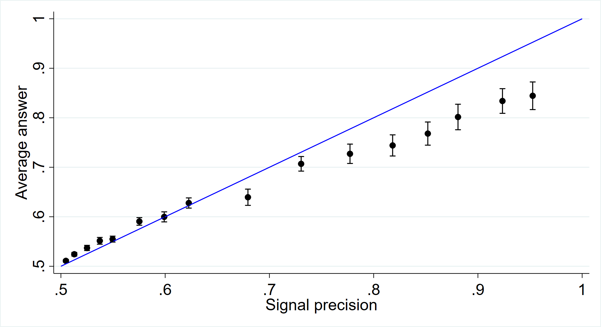
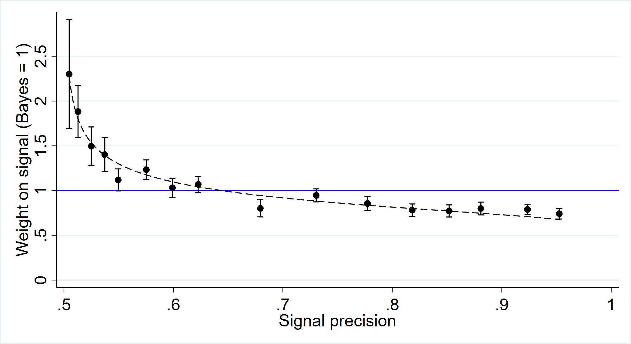
First, we consider how subjects infer from one symmetric signal. Figure 2 presents our main experimental results graphically, comparing our estimates for each condition (black circles) with Bayesian updating (blue lines) and our model’s fitted predictions (dashed lines). Consistent with the theory, subjects systematically overinfer from weak signals and underinfer from strong signals, and the data clearly reject models in which weight is not a function of the Bayesian posterior. The top panel shows that overinference is close to linear in signal strength using a log-log plot, which suggests that the power-law model is a good fit. The middle panel shows that beliefs are increasing but concave in signal precision. The bottom panel provides more evidence that the effect of signal precision on weight is nonlinear. Besides the qualitative explanatory power, the power function from the model in Section 2 predicts the levels of overinference and underinference well.

Figure 2: Over- and Underinference of Symmetric Signals by Signal Strength

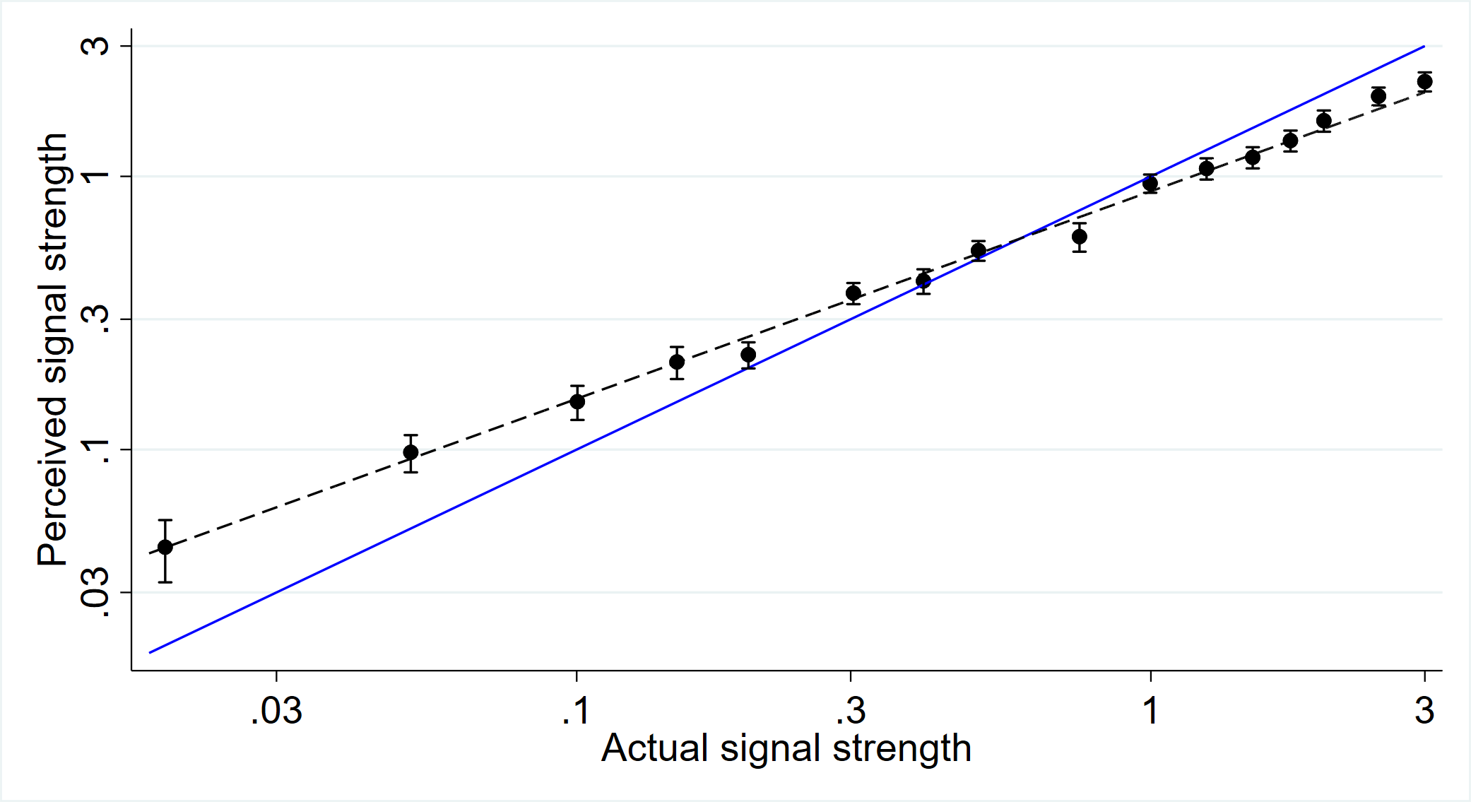
• Notes: The top panel plots signal strength perception as a function of true signal strength on a log-log scale. The middle panel plots the signal strength average answer subjects give as a function of the Bayesian posterior. The bottom panel plots the average weight subjects put on signals relative to a Bayesian. Blue lines indicate Bayesian behavior. The dashed line fits the data with a power weighting function using nonlinear least squares. All panels show that subjects overweight weak signals and underweight strong signals. Observations are winsorized, for each signal strength, at the 5% level. Error bars indicate 95% confidence intervals, clustered at the subject level.

We estimate $p^{*}$ and $\beta$ using nonlinear least squares over signal types $s$:

$$\text{Weight}_{s}=(\text{logit }p^{*})^{-(1-\beta)}\cdot|\text{logit }p_{s}|^{-(1-\beta)}.$$ (5)

The estimated value for $p^{*}$ is 0.64 (s.e. 0.01) and for $\beta$ is 0.76 (s.e. 0.03). The value of $\beta$ is statistically significantly less than one (p-value $<0.001$). These values correspond to an estimate of $k$ of 0.88 (s.e. 0.02). All standard errors are clustered at the subject level.

4.2 Heterogeneity

Average effects mask significant heterogeneities across subjects. Appendix Figure A3 plots the raw cumulative distribution and probability density functions at the individual level. This figure shows that while the majority of subjects overweight weak signals and underweight strong signals, some people are much more susceptible to these misperceptions than others.

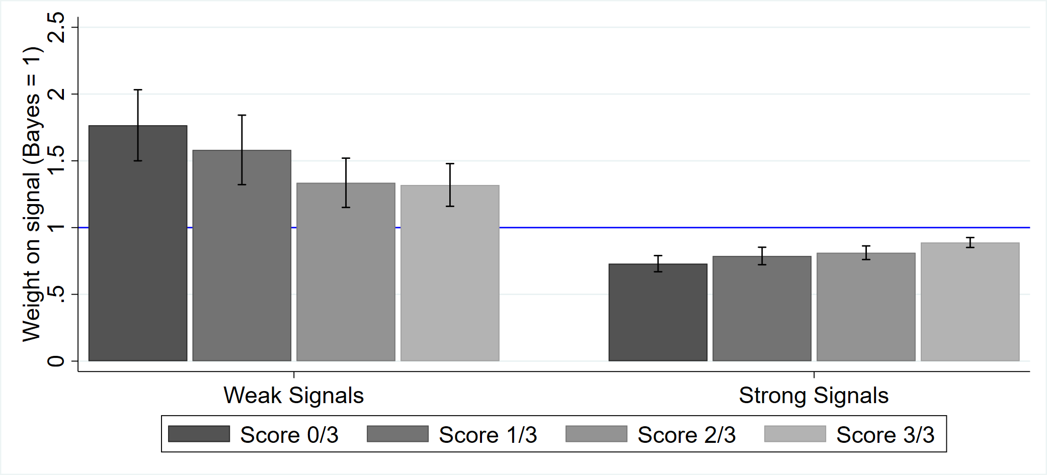
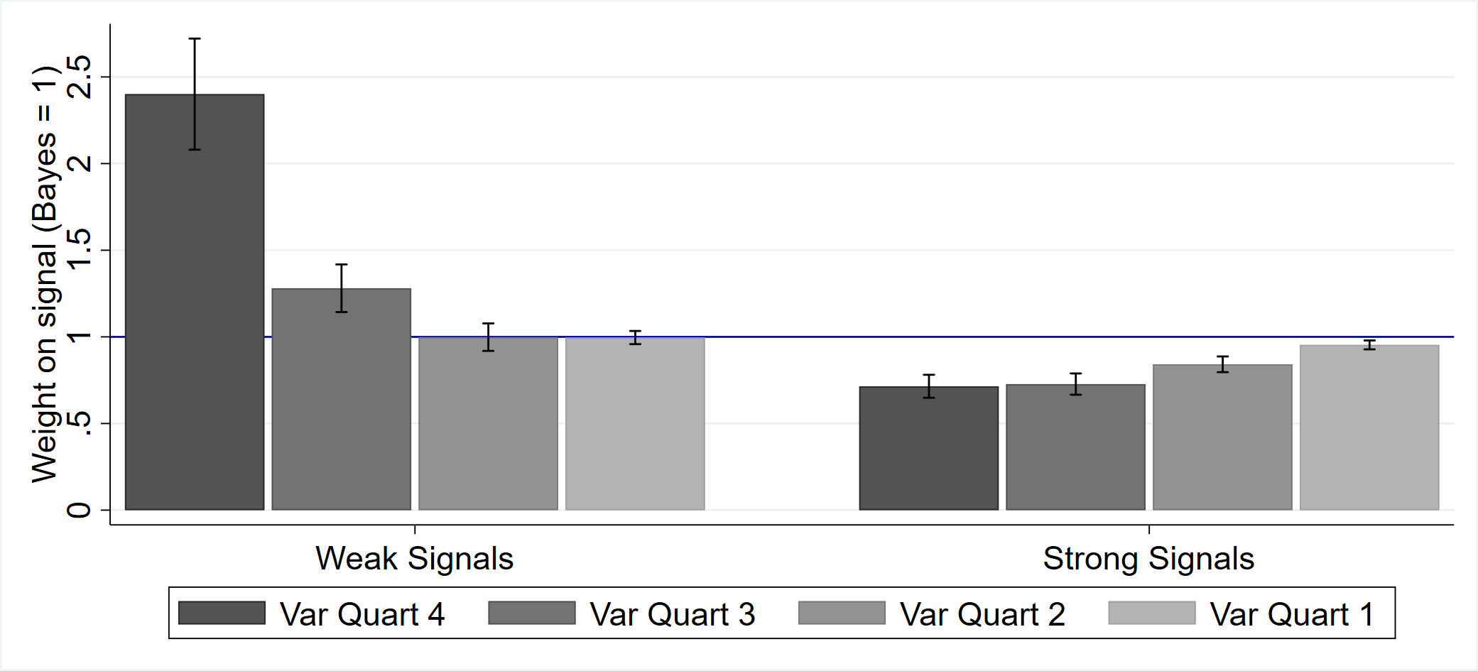
In particular, the types of heterogeneity in treatment effects observed suggest that cognitive sophistication and imprecision are important contributing factors. The three-item cognitive reflection test (CRT) from [30] provides our barometer for cognitive sophistication. The top panel of Figure 3 plots patterns of over- and underinference by CRT score and signal strength. Subjects who score higher on the CRT infer less from weak signals ($p<0.6$) and more from strong signals ($p>0.7$). Moving from a CRT score of 0/3 to 3/3 is associated with a decrease of 0.52 for the weight placed on weak signals (s.e. 0.18, p-value $=0.004$). Meanwhile, this change is associated with an increase of 0.15 weight on strong signals (s.e. 0.043, p-value $<0.001$).

Figure 3: Heterogeneity in Inference from Weak Signals and Strong Signals

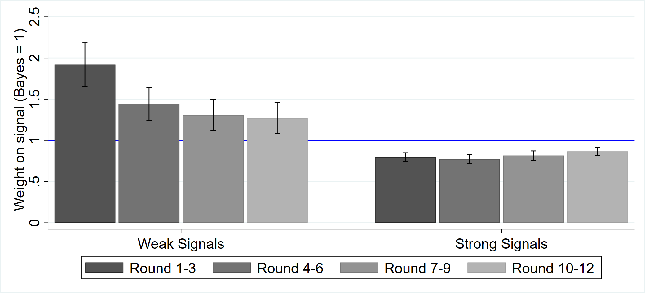
• Notes: In all three panels, the y-axis is weight subjects put on signals. Weak signals have precision between 0.5 and 0.6; strong signals have precision between 0.7 and 1. The top panel plots weight by CRT score. The middle panel plots weight by round in the experiment. The bottom panel plots weight by how much variance the subject has in their answers. Subjects are ranked by variance in weight and split into quartiles; Quart 1 has the least variance. Blue lines indicate Bayesian updating. This figure shows that higher CRT scores, more experience, and lower variance are associated with less weight on weak signals and more weight on strong signals. Error bars indicate 95% confidence intervals.

Subjects may become more cognitively precise as they learn how to interpret more signals, so we next consider how subjects behave over the course of this part of the experiment. Results suggest that there is evidence for learning over the course of the experiment, and the middle panel of Figure 3 plots over/underinference over the course of the twelve rounds. An increase in one round of the experiment is associated with a decrease of 0.074 weight on weak signals (s.e. 0.018, p-value $<0.001$) and an increase of 0.008 weight on strong signals (s.e. 0.004, p-value $=0.039$). Appendix Figure A4 shows similar patterns when comparing subjects who have a higher self-reported level of news consumption; the effects are largely driven by differences in overinference of weak signals.

Finally, one direct proxy for cognitive precision is the variance in subjects’ answers; over the course of the experiment, subjects who have weights that have higher variance are likely to be less cognitively precise, leading them to be less sensitive to the true strength of the signals. The bottom panel of Figure 3 ranks subjects by the variance in their weights in the experiment and plots over/underinference by this ranking. Moving from the 75th percentile in variance to the 25th percentile in variance is associated with a decrease of 0.93 weight on weak signals (s.e. 0.11, p-value $<0.001$) and an increase of 0.17 weight on strong signals (s.e. 0.03, p-value $<0.001$). Note that variance is endogenous to subjects’ signal weight levels, so some of this effect may be mechanical. Both the CRT and news heterogeneity analyses were preregistered, while the variance and round tests were conducted ex post.

We summarize the main and heterogeneous treatment effects in Table 1. The first column effectively restates the main results in Section 4.1. There is a statistically significant negative relationship between signal strength and overinference weight, and the regression model predicts overinference when $\mathbb{S}<0.308/(1.420-1)=0.700$, which corresponds to a switching point of $p=0.668$. Column (2)-(5) describe the heterogeneity results. The interaction between signal strength and CRT score is positive, indicating that the higher the subject’s CRT score, the more they infer as signal strength increases. Similarly, the interaction between signal strength and round number is positive, between signal strength and standard deviation of guesses is negative, and between signal strength and self-reported news consumption is positive. All effects are statistically significant at the 1-percent level.

While Table 1 uses a linear specification, the model suggests that a nonlinear specification may be more appropriate. As such, we show in Appendix Appendix A that results are similar if we estimate a power-law model using nonlinear least squares. The estimate for sensitivity $\beta$ is again significantly below 1, and the heterogeneity-related interaction effects are similar. While the power-law model provides a better fit for the main effect, the specification chosen does not affect the interpretation of any of the results.

Table 1: Effect of Signal Strength on Over- and Underinference

	(1)	(2)	(3)	(4)	(5)
	Main Effects	By CRT Score	By Round	By SD	By News
Signal Strength	-0.308	-0.481	-0.578	0.149	-0.519
	(0.031)	(0.064)	(0.072)	(0.031)	(0.093)
Strength x CRT Score		0.102
		(0.028)
Strength x Round Number			0.042
			(0.009)
Strength x SD of Guesses				-0.430
				(0.038)
Strength x News Cons					0.334
					(0.129)
Constant	1.420	1.421	1.416	1.398	1.420
	(0.030)	(0.030)	(0.030)	(0.021)	(0.030)
Subject FE	Yes	Yes	Yes	Yes	Yes
Round FE	Yes	Yes	Yes	Yes	Yes
Observations	3964	3964	3964	3964	3964
$R^{2}$	0.23	0.23	0.24	0.29	0.23

• Notes: OLS, with standard errors (in parentheses) clustered at subject level. Dependent variable is the weight put on the signal compared to a Bayesian (as defined in Equation 2.) Weights greater than 1 correspond to overinference; weights less than 1 correspond to underinference. Column (1) shows that subjects overinfer from weak signals (since the constant is greater than 1) and that overinference declines for stronger signals. Columns (2)-(5) show heterogeneity across CRT score, round number, standard deviation of over/underweighting, and news consumption, respectively. CRT score ranges from 0 to 3. Round number ranges from 1 to 12. News consumption ranges from 0 to 1.

4.3 Multiple Signals

When subjects receive multiple signals, they weight the signals less than if they receive one signal, as is consistent with past literature (as discussed in [11] and [13]). Appendix Figure A1 shows that subjects put less weight on multiple signals than on one signal, holding the Bayesian posterior fixed. This comparison holds both when signals are all in the same direction and when they are mixed.

These results extend the findings of [39] by showing that people misperceive both the strength and the quantity of signals. When misperceptions about quantity play a larger role than misperceptions about signal strength, there is a downward shift of the curves when people receive multiple signals.

4.4 Demand for Information

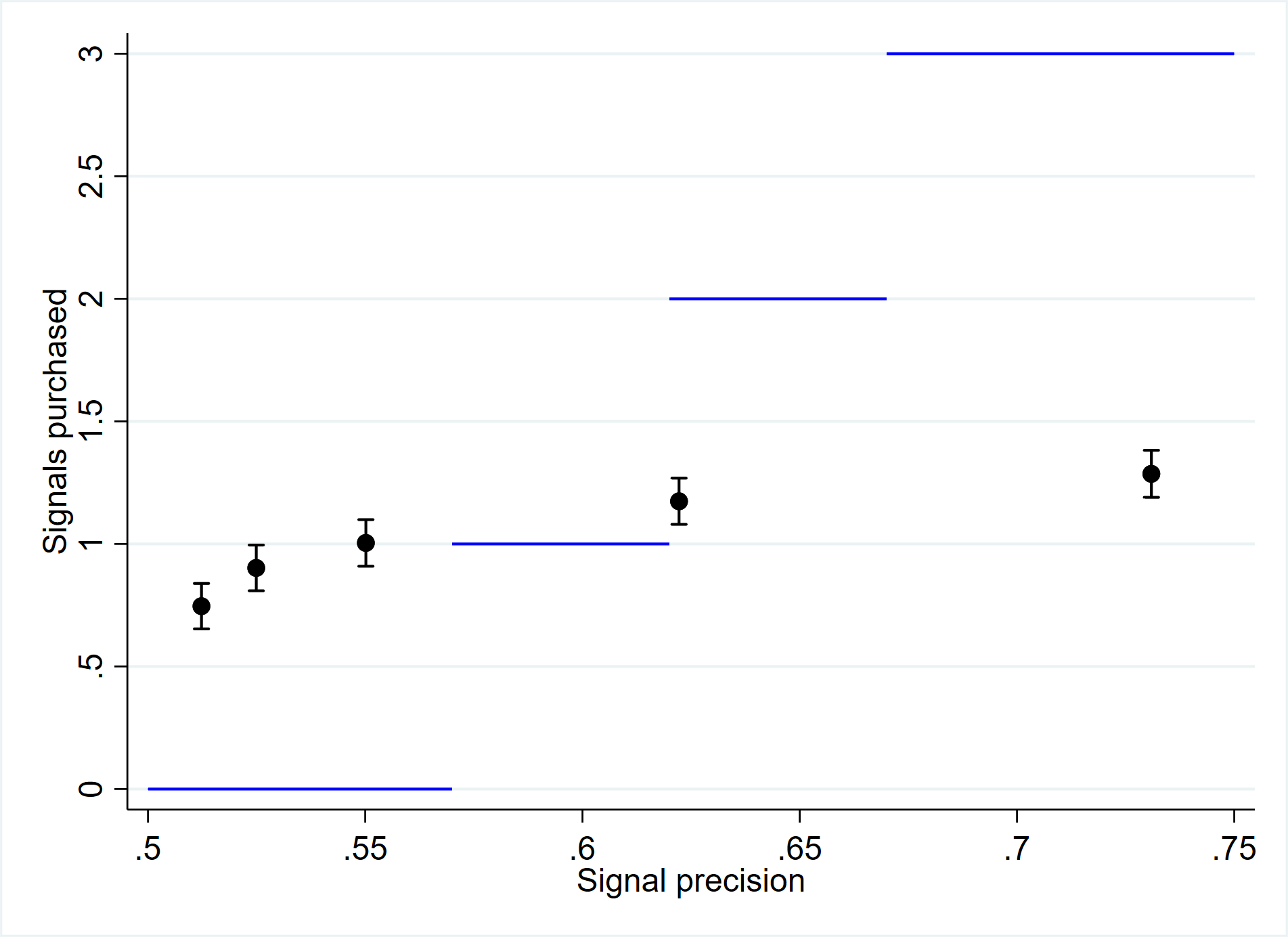
Patterns of overinference and underinference also lead to demand for information that is too high or too low relative to the optimum. Figure 4 plots the average number of signals purchased as a function of each signal strength, comparing subject behavior to the optimal choice if subjects were Bayesian and only valued signals for their instrumental value.

Figure 4: Number of Signals Purchased

• Notes: This figure plots the number of signals purchased as a function of signal precision. The blue lines correspond to the payoff-maximizing number of signals purchased. This figure shows that subjects over-purchase weak signals and under-purchase strong signals. Error bars indicate 95% confidence intervals.

As can be seen in the figure, subjects systematically over-purchase weak signals and under-purchase strong signals. The cost of a signal that leads a Bayesian to form a posterior of less than 0.57 outweighs its benefit; however, the majority of subjects purchase at least one signal when $p=0.55$ and $p=0.525$. Additionally, 81 percent of subjects purchase fewer than the optimal level of three signals when $p=0.73$.

There are other reasons for purchasing signals that are orthogonal to inference. For instance, subjects may be curious to learn the card draw itself, leading them to demand information for its own sake (as in [34]), raising the curve. Subjects’ answers are constrained to be between 0 and 3, so they may prefer to select interior answers, flattening the curve. These effects do not fully explain the results but may contribute to the extremeness. For instance, more subjects purchase zero or one signals when $p=0.73$ than purchase two or three, which cannot be fully explained by curiosity or interior guesses. There is also suggestive evidence that differences in signal purchasing is partly explained by differences in inference at the individual level: subjects who purchase more signals on average have posteriors that move 0.49 pp further (s.e. 0.32 pp, $p=0.124$) on all other questions.

4.5 Mechanisms

Overreaction and underreaction could be driven by misperceptions of signal strength or driven by misperceptions of probabilities that happen to be close to 1/2. For instance, if $p_{1}=0.505$ and $p_{2}=0.495$, overinference may be due to misperceptions of weak signals or due to the fact that $p_{1}$ is only slightly greater than $1-p_{1}$. To disentangle these hypotheses, we compare behavior in the treatment asymmetric signals when $p_{1}=0.505$ and $p_{2}=p_{H}$ to behavior when $p_{1}=0.495$ and $p_{2}=p_{H}$, where $p_{H}\gg 0.5$.

We find that misperceptions of signal strength explains these findings better. Subjects do not systematically infer differently when $p_{1}=0.505$ and $p_{1}=0.495$. When $p_{1}=0.505$, the average $\beta$ is 0.54 (s.e. 0.05). When $p_{1}=0.495$, the average $\beta$ is 0.60 (s.e. 0.05). The difference is not statistically significant (-0.06, s.e. 0.07, p-value $=0.404$) and the point estimate is in the opposite direction of that of the alternative model.

Next, we consider how people respond to signals of uncertain strength. Misperceiving people may apply their weighting function and signal combination in one of two ways. They might either first combine the signals and then weight the combined signal, or they may first weight the signals separately and then combine the weighted components.

Consider a signal that either leads a Bayesian to a posterior of $p_{L}\gtrless 1/2$ or $p_{H}>\max\{p_{L},1-p_{L}\}>1/2$, each with probability 1/2. Denoting by $\hat{p}$ the agent’s posterior, the “combined signals” model predicts $\text{logit}(\tilde{p})=K\cdot(\text{logit}[(p_{L}+p_{H})/2)]^{\beta}$. The “separate signals” model predicts $\text{logit}(\tilde{p})=1/2\cdot\left[k*(\text{logit}(p_{L}/2))^{\beta}+K*(\text{logit}(p_{H}/2))^{\beta}\right]$ when $p_{L}>1/2$ and $\text{logit}(\tilde{p})=1/2\cdot\left[-k*(\text{logit}((1-p_{L})/2))^{\beta}+k*(\text{logit}(p_{H}/2))^{\beta}\right]$ when $p_{L}<1/2$. These models make noticeably different predictions when $p_{L}$ is close to 1/2. The combined signals model predicts smooth behavior and a higher $\tilde{p}$, while the separate signals model predicts a kink at $p_{L}=1/2$ and a lower $\tilde{p}$.

In the experiment, subjects receive $(p_{L}=0.505$, $p_{H}=0.807)$ or $(p_{L}=0.495$, $p_{H}=0.817)$. The Bayesian model predicts posteriors of 0.656. Using the estimated parameters as before ($\beta=0.760$ and $k=0.882$), the combined signals model predicts near-Bayesian posteriors of 0.653 in each case. Meanwhile, the separate signals model predicts underinference and asymmetry, with a posterior of 0.636 when the signals are both larger than 0.5 and 0.628 when they are in opposite directions.

Empirically, the separate signals model fits the data best. The fit is better for both levels and differences. Subjects’ posteriors are 0.620 (s.e. 0.057) when the signal directions are aligned and 0.609 (s.e. 0.054) when they are misaligned. In fact, subjects underinfer slightly more than the separate signals model predicts (see [51] for one possible explanation). Underinference is suggestively more severe when the directions are misaligned (p-value $=0.106$) and the point estimate for this difference is similar to that of the theoretical prediction. The difference in behavior from combined and separate signals also indicates that subjects’ behavior is inconsistent with [21]’s (C-WP) framework of divisible updating.

4.6 Robustness

This section considers three alternative hypotheses for these results that are unrelated to over- or underinference.

First, it is possible that subjects dislike stating “50 percent” even when signals are very uninformative. There is no systematic evidence for this. Among the 72 subjects who see a completely uninformative signal (where the decks each have 832 Diamonds and 832 Spades), 69 of them (96 percent) give an answer of exactly 50 percent.

Second, it is possible that subjects are systematically more inclined to prefer Green over Purple, or attend more to Diamonds over Spades, or vice versa. If this were the case, then subjects may overinfer in one direction and underinfer in the opposite direction by a different amount, leading to average misinference. However, there is no evidence of color asymmetry; subjects’ average estimate of P(Green) is 0.503 (s.e. 0.002). There is also no evidence for suit asymmetry; on average, subjects’ signal weight is 1.156 (s.e. 0.031) when they see a Diamond and 1.134 (s.e. 0.035) when they see a Spade.

Third, it is possible that something about the particular number of cards in the deck leads subjects to misperceive signal strength. For instance, they may have a left-digit bias ([64]). Recall that for the one-signal questions, the deck size was randomly either 1,665 or 337. The deck size leads to a statistically significant shift in the estimated switching point $p^{*}$ but not in the sensitivity $\beta$: $p^{*}$ for the larger deck is 0.68 (s.e. 0.02) and $\beta$ is 0.75 (s.e. 0.03); $p^{*}$ for the smaller deck is 0.61 (s.e. 0.01) and $\beta$ is 0.77 (s.e. 0.04). With each deck size, $\beta$ is statistically significantly less than 1 ($p$-values $<0.001$).

It is possible that these factors have modest quantitative effects on the main estimates, but they cannot entirely explain the results.

5 Evidence from Finance and Sports Betting

While the experimental setting is tightly controlled, its abstract features naturally raise questions of external validity. To test the implications of our theory in more realistic high-stakes settings, we therefore now consider evidence from a set of sports betting markets and financial markets. Departing from the experimental environment comes at a cost, as we no longer have direct knowledge of the true DGP or the informativeness of specific signals to which prices are responding. But we choose a set of markets to analyze so as to obtain close proxies for signal informativeness under minimal assumptions: we consider the prices of binary bets (with payouts of either $0 or $1) with known terminal horizon, for which we can construct proxies for signal informativeness under the null of Bayesian updating. By considering price movements across informativeness regimes, we test whether the patterns of overinference vs. underinference documented in the experiment apply in this real-world financial-market setting. We first describe our setting and estimation strategy in more detail, before turning to our empirical results.

5.1 Conceptual Setup

To set the stage for our empirical analysis, we first describe the conceptual framework that we then take to the data. This section builds closely on [5] (AR AR21) and [4] (AL AL-WP) to generalize Section 2 to handle multiple periods with arbitrary signals. Time is indexed by $t=0,1,2,\ldots,T$. As before, there is a binary state $\theta\in\{0,1\}$. Each period, a person observes a signal $s_{t}$ drawn from arbitrary distribution $DGP(s_{t}\,|\,\theta,H_{t-1}),$ where $H_{t}\equiv\{s_{1},s_{2},...\}$ is the history of signal realizations. The person’s belief in state 1 at time $t$ given the DGP and history $H_{t}$ is denoted by $\pi_{t}(H_{t})$ (or $\pi_{t}$ for short). The belief stream $\bm{\pi}$ refers to the collection of the person’s beliefs over time.

While we cannot directly test for overinference vs. underinference without knowledge of the DGP, keeping track of the following two objects will allow for well-motivated indirect tests. First, define the movement of a belief stream from period $t_{1}$ to $t_{2}>t_{1}$ as the sum of squared changes of beliefs over these periods:

$$m_{t_{1},t_{2}}(\bm{\pi})\equiv\sum\nolimits_{\tau=t_{1}}^{t_{2}-1}(\pi_{\tau+1}-\pi_{\tau})^{2}.$$

Then, defining the uncertainty of belief at period $t$ as $u_{t}(\bm{\pi})\equiv(1-\pi_{t})\pi_{t}$, we define uncertainty reduction from period $t_{1}$ to period $t_{2}>t_{1}$ as:

$$r_{t_{1},t_{2}}(\bm{\pi})\equiv\sum\nolimits_{\tau=t_{1}}^{t_{2}-1}(u_{\tau}(\bm{\pi})-u_{\tau+1}(\bm{\pi}))=u_{t_{1}}(\bm{\pi})-u_{t_{2}}(\bm{\pi}).$$

For each variable, we define the concomitant random variable in capital letters (e.g., $M_{t_{1},t_{2}}$).

Under the null model of Bayesian updating, beliefs satisfy $\pi_{t}(H_{t})=\mathbb{E}[\theta\,|\,H_{t}]$ for all $H_{t}$, where $\mathbb{E}$ is the expectation under the true (physical) measure. We denote $\mathbb{E}_{t}[\cdot]=\mathbb{E}[\,\cdot\,|\,H_{t}].$

The Equality of Movement and Uncertainty Reduction

As in AR (AR21), the martingale property of beliefs under the null implies that, regardless of the DGP, expected Bayesian belief movement from any period $t_{1}$ to period $t_{2}$ must equal expected uncertainty reduction:

Proposition 2 (Movement and Uncertainty Reduction).

Assume $\pi_{t}(H_{t})=\mathbb{E}_{t}[\theta]$. For any DGP and for any periods $t_{1}$ and $t_{2}$, $\mathbb{E}_{t_{1}}[M_{t_{1},t_{2}}]=\mathbb{E}_{t_{2}}[R_{t_{1},t_{2}}].$

This result formalizes the “correct” amount of belief volatility (or movement) under rationality, without the need to know the true unobservable DGP. One can then follow AR (AR21) to use this result as the basis for a statistical test for Bayesian updating: given a set of belief streams, one can calculate the difference between movement and uncertainty reduction (which they call “excess movement”) and then apply a means test to see if the average difference is statistically different from zero. If so, one can reject — with a certain confidence level — that the beliefs arose from Bayesian updating. This result thus provides a testable link between belief movement, uncertainty reduction, and signal informativeness: when we observe a Bayesian person’s beliefs moving, this must (on average) mean that she is receiving informative signals and reducing her uncertainty accordingly.

We emphasize two crucial features of this test: (1) it is valid regardless of the DGP, and (2) it can be applied to arbitrary belief substreams (from period $t_{1}$ to $t_{2}$), as Proposition 2 applies ex ante in all cases. Thus, given some ex ante known and observable sorting variable related to signal strength, we can test whether excess movement is related to signal strength. We will use time to resolution ($T-t$) as our separating variable, and we discuss its relation to signal strength — and the relation of excess movement to over- and underinference — below.

Underreaction and Overreaction

There is a natural connection between excess movement and overreaction: people who overreact are intuitively moving around “too much” relative to the informativeness of signals. AR (AR21) formalize this connection. In particular, Proposition 6 of that paper demonstrates that in a two-period environment, a person with a correct prior who overinfers from signals will exhibit a positive excess movement statistic, while a person who underinfers will exhibit a negative statistic. Proposition 7 then demonstrates that the same relationship holds over many periods in a simple symmetric binary-signal environment (even though the person no longer necessarily has the correct beliefs in later periods). With other DGPs, however, it is challenging to obtain general analytic results. Consequently, we turn to simulations to confirm the intuition that the same intuitive relationships hold under our updating model in environments that more closely map to our empirical setting.

5.2 Simulated Belief Streams

We use simulations to understand basic patterns in movement and uncertainty reduction for a person who updates using our model in Section 2 when forming beliefs about the outcome of a sporting event or the future level of the stock market. These settings feature similar signals (points scored, daily returns) received in each period, with the aggregate of that information determining the final state. To transparently model such situations, we consider a simple DGP in which there are two “teams” representing the two states, exactly one team scores in each of $T$ periods, each team has equal probability of scoring in each period, and the final state is which team has the highest score after the final period. For example, if a team is leading by one score with 2 periods left, they have a 75% chance of being the final winner because they win if they score in one of the final 2 periods.

Figure 5: Simulated Movement and Uncertainty Reduction Over Time For Different Models

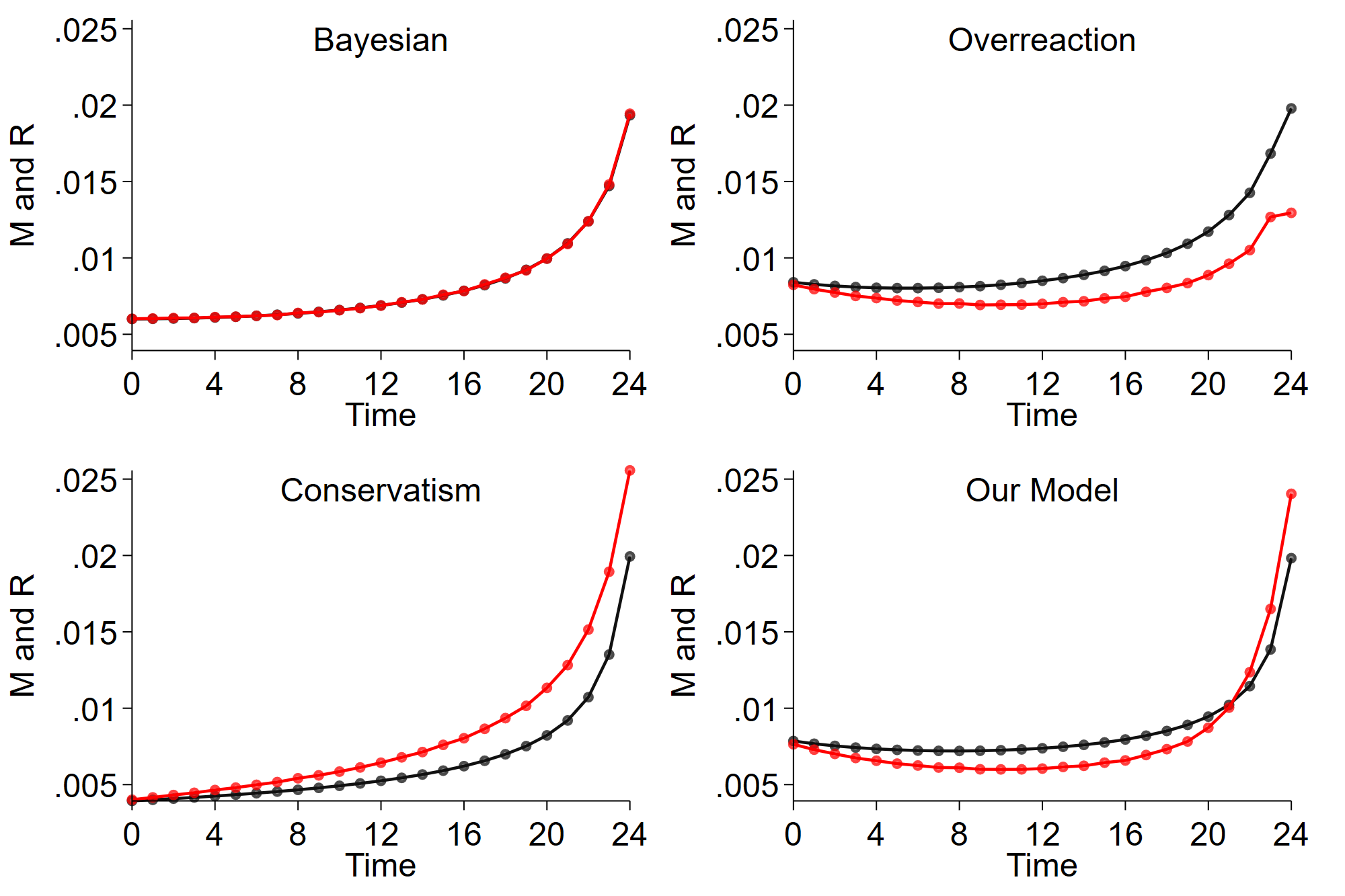
• Notes: This figure shows the average movement (black line) and uncertainty reduction (red line) statistics over time for four different models, averaged over 1 million simulations of the game-like DGP discussed in the text with $T=27$. The updating models are (1) Bayesian updating (the signal strength is correctly perceived as $\mathbb{S}$), (2) conservatism (the perceived signal strength is $0.8\cdot\mathbb{S}$), (3) overreaction (the perceived signal strength is $1.2\cdot\mathbb{S}$), and (4) our model (the perceived signal strength is $k\cdot\mathbb{S}^{\beta}$ with $k=0.882$ and $\beta=0.760$). For Bayesian updating, these statistics are always equal. For conservatism, movement is always less than uncertainty reduction, and the opposite is true for overreaction. For the misperceiving person in our model, movement is greater than uncertainty reduction in early time periods (where signals are generally weak) and lower in later time periods (where signals are generally strong).

The top-left panel of Figure 5 shows the expected movement and uncertainty reduction statistics over time for a Bayesian (calculated from one million simulations of this DGP). First, as predicted by Proposition 2, the statistics are equal at each period. Next, note that both statistics are rising as the resolution of the game approaches. The initial periods always contain very little information, while the later periods sometimes contain no information (because one team has an insurmountable lead) and sometimes contain a large quantity of information (because the scores are very close). Overall, though, signal strength rises over time, and average movement and uncertainty reduction increase accordingly. As we show shortly, this pattern will also hold in all of our empirical settings.

What do the statistics look like for misperceiving people? Following intuition and the theoretical results from simpler DGPs, overreaction (top-right panel) leads to positive excess movement in every period, while the opposite is true for underreaction (bottom-left panel). The bottom-right panel displays the results for our model, with parameters estimated from our experiment as in Section 4.1 ($\beta=0.760,k=0.882$). In the early periods, average signal strength is low, leading to overreaction, which in turn generates excess movement. In later periods, the amount of information revealed is higher, leading to underreaction. Belief movement increases, but not in line with the increase in uncertainty reduction. There is therefore a switching period at which average movement crosses below uncertainty reduction. This pattern is consistent with our model, but it does not occur under Bayesian updating or when there is universal overreaction or underreaction.

5.3 Sports Betting Data

Data Description

We start with data on sports betting. Our data comes from Betfair, which operates a large prediction market in which individuals are matched on an exchange to make opposing financial bets about the outcome of a sporting event. As in a standard centralized financial exchange, one can observe time-stamped transaction prices — determined by supply and demand — for a contract in which one party pays another a set amount given a particular realized outcome of the game. These are the same data as used in AR (AR21), and we use the same sample (2006–2014) and data filters (discussed further below) as in that paper.

Given our focus in this section on equilibrium bet-price data, we follow the literature that interprets these prices as “market beliefs.” An excess movement test based on Proposition 2, therefore, can be viewed in this setting as a test of the joint null that market prices may be interpreted as beliefs and that these beliefs are Bayesian. But while this might affect the interpretation of full-sample excess movement tests, it poses less of a problem for our purposes. We are fixing the environment (i.e., the particular betting market in question) and comparing excess movement as one varies the signal strength (proxied by time to maturity) within this environment. If we assume that the mapping from individual to market beliefs does not change systematically within a stream as one moves closer to maturity, our findings are at minimum directionally informative about both individual and market-level reactions to information across signal-strength regimes.

We focus on markets for five major sports (soccer, American football, baseball, basketball, and hockey), and we restrict attention to contracts over the final winner of the game (and omit more exotic contracts, such as which team will be winning at the midpoint and the number of goals scored). We use observations only when the game is being played. To remove extremely high-frequency noise, we follow AR (AR21) and keep at most one observation per minute, and also drop observations with less than 1% of average volume. Finally, we attempt to have similar timing in events by dropping (less common) events in a category for which the timing of the game is different (such as WNBA games, in which the game time is shorter than the NBA).

Graphs of Movement and Uncertainty Reduction

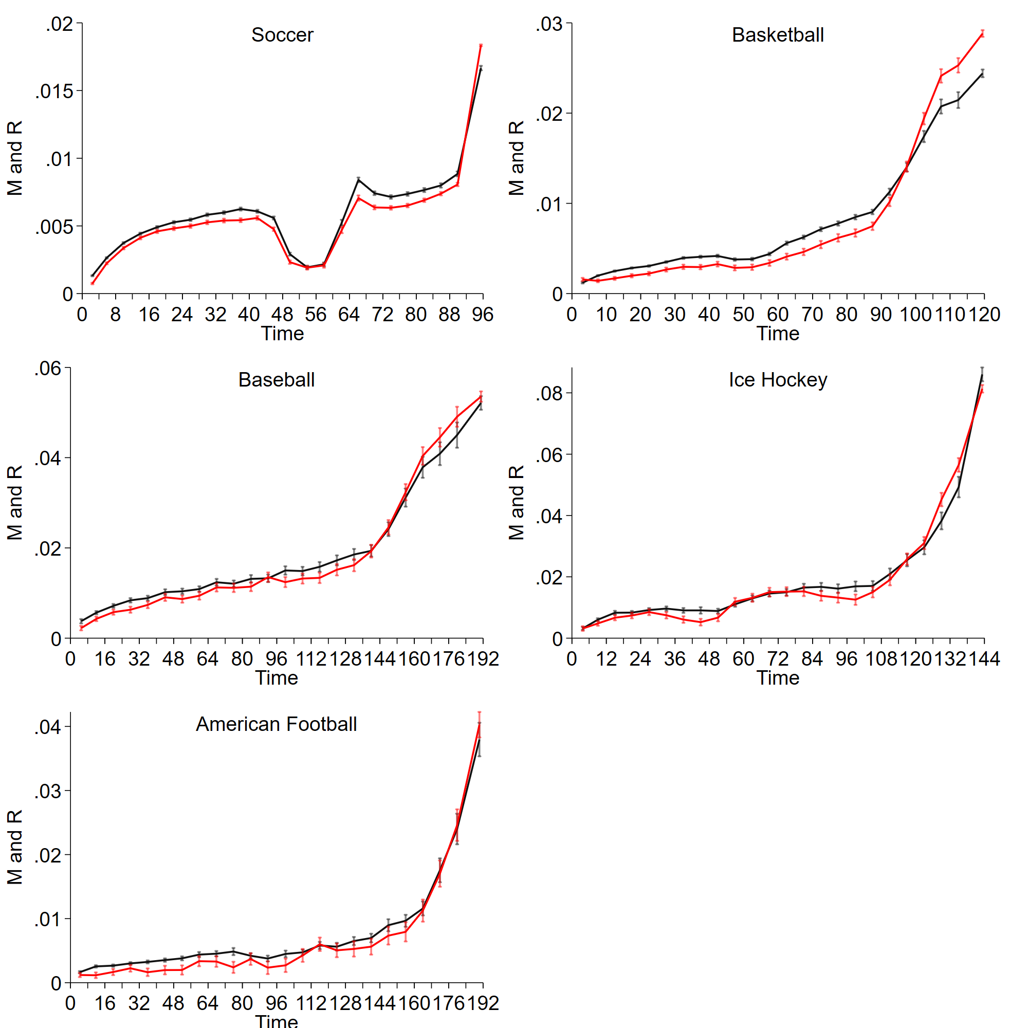
Figure 6 shows average movement and uncertainty reduction (as well as confidence intervals) across time for each sport. Observations occur in continuous time and therefore must be aggregated in some way. Our data contain clock-time (“1:31pm”) rather than game-time (“4:50 through the third quarter”) observations; we therefore consider average movement and uncertainty reduction for observations within 24 time chunks, each of which corresponds to $1/24$ the length of an average game. As in the simulations, average movement and uncertainty reduction are generally increasing over time (with the exception of mid-period breaks). Early in games for each sport, movement is greater than uncertainty reduction, and for each sport there is a time at which movement drops below uncertainty reduction. For four of the five sports, movement then continues to be lower than uncertainty reduction after this time (for hockey, movement stays lower than uncertainty until the final period). The market accordingly appears to overreact to the less-informative signals at the beginning of a game, and underreact to the more-informative signals at the end of a game.

Figure 6: Movement and Uncertainty Reduction Over Time for Different Sports

• Notes: This figure shows the average movement (black line) and uncertainty reduction (red line) statistics over time for five different sports (as well as 95% confidence intervals). In each case, movement is greater than uncertainty reduction in early time periods and then drops below in later time periods.

Statistical Tests

Are the patterns in the figures statistically meaningful? To answer this question, we require a test to determine if there is overreaction (captured by expected movement being greater than uncertainty reduction) when signals are weak (captured by low uncertainty reduction), and underreaction when signals are strong. We therefore regress average movement in each period on average uncertainty reduction in each period. Under the null hypothesis of Bayesian updating, the constant will be equal to 0 and the slope coefficient equal to 1, as average movement should be equal to average uncertainty reduction in every period. However, for a misperceiving person who updates according to our model, average movement will be higher than average uncertainty reduction when reduction is low, but lower than uncertainty reduction when reduction is high, such that the constant will be positive and the slope coefficient will be less than one.

The results for these regressions are shown in the first five columns of Table 2. Given that the regressions use calculated averages, we bootstrap standard errors by resampling events with replacement and recalculating averages 10,000 times (OLS standard errors are very similar). For each sport, the slope and constant coefficients are highly statistically significantly different from the Bayesian benchmark in the direction predicted by the theory: we consistently observe evidence for overinference from weak signals (when average uncertainty reduction is low) and underinference from strong signals (when reduction is high).

To understand the magnitude of the estimates, note that beliefs moving 3 percentage points up and then 3 points down would produce movement of 0.0018 (close to the average constant coefficient) and no uncertainty reduction. Given this average constant, the average slope coefficient then implies that movement will cross uncertainty reduction when both are around 0.014, which corresponds to one belief movement of around 12 percentage points.

Table 2: Regressions of Movement on Uncertainty Reduction

Dep Var:	Sports					Finance
Movement	Soccer	Basketball	Baseball	Hockey	Football	Raw	Risk-Adj.
Uncert. Red.	0.918	0.806	0.889	0.945	0.912	0.680	0.733
	(0.005)	(0.008)	(0.013)	(0.013)	(0.027)	(0.040)	(0.041)
Constant	0.0009	0.0018	0.0026	0.0018	0.0015	0.0065	0.0060
	(0.0001)	(0.0001)	(0.0002)	(0.0002)	(0.0002)	(0.0003)	(0.0003)
$R^{2}$	0.977	0.985	0.995	0.976	0.995	0.944	0.941
Time Chunks	24	24	24	24	24	24	24
Events	6,584	5,176	3,927	4,123	1,390	955	955
Observations	4,589,289	867,567	166,346	109,751	86,193	58,864	58,864
$p$-val.: $\beta_{1}=1$	<0.001	<0.001	<0.001	<0.001	0.007	<0.001	<0.001
$p$-val.: $\beta_{0}=0$	<0.001	<0.001	<0.001	<0.001	<0.001	<0.001	<0.001

• Notes: This table presents the results from OLS regressions (with bootstrapped standard errors in parentheses) of average movement in a time period on average uncertainty reduction for five sports and the options data.

Note that we are regressing the average movement in a time chunk on the average uncertainty reduction. We do this because, for a Bayesian, the expected movement at any time $\mathbb{E}_{t}[M_{t,t+1}]$ must equal the expected uncertainty reduction $\mathbb{E}_{t}[R_{t,t+1}]$. However, any individual belief change does not yield movement and reduction equal to these expectations, but rather equal to these expectations plus a mean-zero error term. Therefore, if we simply regressed all the (unaveraged) movement statistics on the (unaveraged) uncertainty reduction statistics, there would be significant attenuation bias due to error in the independent variable. By taking the average over thousands of belief changes at a given time horizon, we are able to estimate the expectation at that time plus a tiny error term, effectively eliminating this bias. In our case, the estimated variance of the error term at each period is more than 100,000 times smaller than the estimated variance of the independent variable, such that the attenuation bias is negligible. Note that the $R^{2}$ values in all cases are very close to 1: variation in movement can be explained almost entirely by variation in uncertainty reduction, but only when the coefficient is less than one.

5.4 Index Options Data

Data Description

The sports betting data provide a useful lab for studying beliefs in an incentivized setting, but they come naturally with some limitations: trading budgets are capped, and payoffs are unrelated to macroeconomically relevant outcomes. So we now consider market-implied beliefs data from a large-scale financial market of first-order importance: options on the S&P 500 index, which are effectively bets on the value of the market index as of some fixed future expiration date. As in AL (AL-WP), we obtain data from OptionMetrics on S&P index option prices with all available strike prices and expiration dates traded on the Chicago Board Options Exchange (CBOE). The sample of trading dates is 1996–2018. We use daily (end-of-day) data, and we implement the same data filters as described in AL (AL-WP); see Section B.1 for further details.

Converting Option Prices to Market-Implied Beliefs

On any given trading date $t$, there are prices for a wide range of S&P options with the same expiration date $T$. The options differ only in their strike prices $K$ (for a call option, the minimum S&P index value at which the option will obtain a positive payoff at expiration). The set of option prices for a given $(t,T)$ pair can thus be translated, using standard methods following [19], into a market-implied (or risk-neutral) probability distribution over the future S&P price on the option expiration date.

Unlike in the case of sports betting data, index options have payoffs that are tied (by construction) to the value of aggregate wealth. Option prices therefore reflect risk aversion in addition to subjective probability assessments about the future index value. This is the main complication in using option-implied probability distributions: they do not, in general, correspond to any notion of aggregate subjective beliefs. (They are equivalent to subjective beliefs only in the case of risk neutrality over the index value, which motivates referring to them as risk-neutral beliefs.) For example, suppose that there are two possible date-$T$ macroeconomic states that are perceived by investors as equally likely. If investors value a marginal dollar in the “bad” state (when the market is low) more than in the “good” state (when the market is high), they will be willing to pay more for the option that pays off in that state. If these risk preferences are not taken into account, one will (falsely) conclude that investors believe that the bad state is more likely.

Addressing this issue is the main theoretical task taken up in AL (AL-WP). That paper shows that under certain assumptions, one can place a bound on excess movement in risk-neutral (RN) beliefs under the null that underlying subjective beliefs are rational. The bound is tight in the space of possible DGPs — that is, one can construct a DGP under which it holds exactly — but it is not necessarily tight under the true real-world DGP. We therefore provide two sets of results in the current analysis, (1) using the raw RN beliefs, and alternatively (2) translating these beliefs to a set of physical (subjective) beliefs under an assumption on risk aversion. For (2), we consider multiple possible assumptions in translating from risk-neutral to physical beliefs, detailed in Appendix B.2. While the hundreds of possible assumptions and parameterizations matter in determining the physical belief estimated for a given risk-neutral belief, their effect on our movement and uncertainty-reduction statistics is so small as to be nearly indetectable. We therefore report results here under our main translation, which assumes a representative investor with power utility over the terminal index value. For robustness, we present estimates under a wide range of alternative parameterizations in Appendix Figure A9, finding that these choices have little effect on our results.

To implement our measurement of RN beliefs, we follow AL (AL-WP) and partition the state space of possible date-$T$ index values into discrete ranges. To maintain the same set of states across expiration dates $T$, we set the states to correspond to ranges for the log return on the S&P 500 from the first observable option trading date to the expiration date. There are 9 potential terminal return states $\theta_{j}$, with $\theta_{1}$ realized if the log return in excess of the risk-free rate is less than $-0.2$ (roughly -20%); $\theta_{2}$ if the log excess return is in the range $(-0.2,-0.15]$; $\theta_{3}$ if $(-0.15,-0.1]$; and so on, so that each state (aside from the extreme states $\theta_{1}$ and $\theta_{9}$, which we discard in our analysis) corresponds to a five-percentage-point range for the S&P’s excess return. The RN belief distribution is then the option-price-implied conditional (date-$t$) probability distribution over each of these 9 states. We measure this distribution for each trading date $t$ until option expiration, at which point we assign probability 1 to the observed realized return state for the S&P 500. We again aggregate the data into 24 time chunks by trading days to expiration, and we average movement and uncertainty reduction statistics using beliefs over all states $\theta_{j}$ for $j=2,\ldots,8$.

Graphs of Movement and Uncertainty Reduction

Figure 7 shows average movement and uncertainty reduction over time in the options data, analogous to Figure 6. The left panel shows the average movement and uncertainty reduction statistics for the raw risk-neutral beliefs, and the right panel shows the statistics for physical beliefs obtained under the main risk adjustment procedure. Time is in trading days, with date 0 normalized to roughly 100 trading days from expiration (there are longer-horizon options for which the same results hold, but we choose to cut off the graph at 100 days for readability). In both cases, movement is consistently above uncertainty reduction relatively far from expiration, when signals are only very weakly informative and uncertainty reduction is statistically indistinguishable from zero. Uncertainty reduction increases dramatically closer to expiration (when market movements are more informative regarding the true index value at the expiration date); while option-implied belief movement increases alongside uncertainty reduction, it appears to do so less than one for one, with uncertainty reduction crossing above movement roughly  10 days from expiration. The patterns observed in this high-stakes financial market are similar to those in the sports betting data for many sports plotted in Figure 6. They are also strikingly similar to the simulated results from our theoretical framework plotted in the bottom-right panel of Figure 5. Recall that these simulations are parameterized using the estimates from our experimental data, so the theory accordingly helps unify the evidence obtained in both the lab and real-world data.

Figure 7: Movement and Uncertainty Reduction Over Time for Finance Data

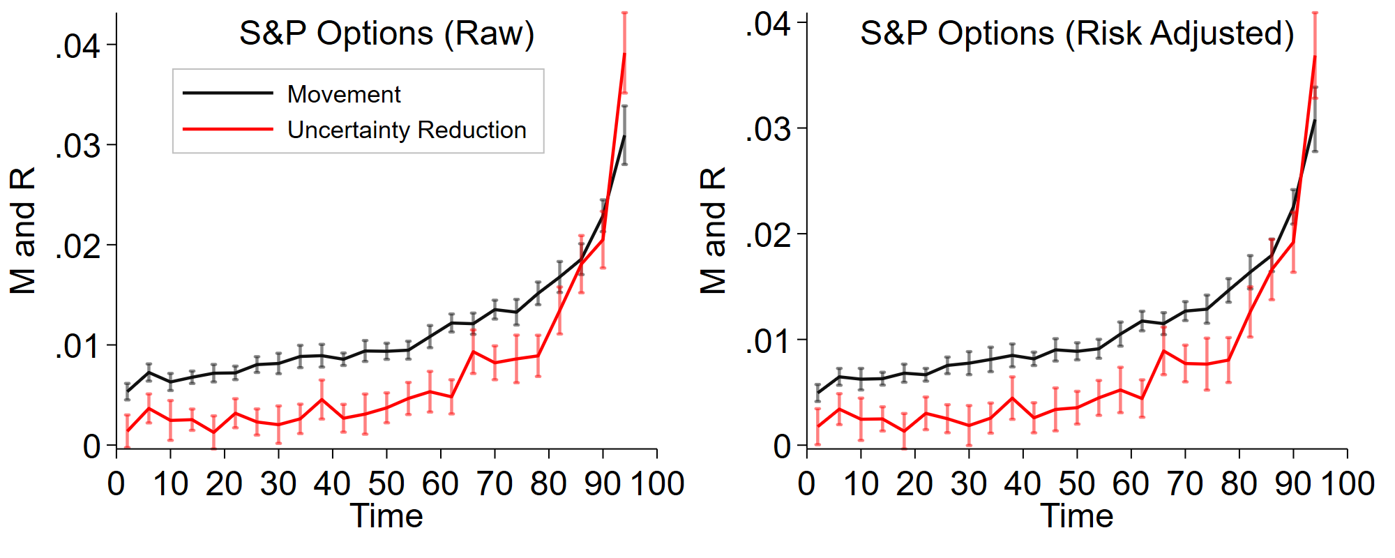
• Notes: This figure shows the average movement (black line) and uncertainty reduction (red line) statistics over time for the beliefs implied by option data (with 95% confidence intervals). The left-hand panel uses the implied unadjusted (risk-neutral) beliefs. The right-hand panel uses a risk adjustment described in the text. Movement is greater than uncertainty at the start of the contract. At the later stages, movement is lower than uncertainty reduction.

Statistical Tests

We conclude this analysis by conducting the same formal tests as in the previous case, regressing average movement on average uncertainty reduction in each time chunk. The results are shown in the final two columns of Table 2. For both the raw and risk-adjusted data, the estimated slope and constant are again highly statistically significantly different from the Bayesian benchmark in the direction predicted by our theory. The positive constant again indicates overreaction when signal informativeness (uncertainty reduction) is low, as movement is significantly positive in these cases; meanwhile, the slope being less than one (and numerically nearly identical to the estimated slope in the sports betting data) indicates underreaction for high enough levels of signal informativeness. The market therefore appears to misperceive in the way predicted for individuals modeled in Section 2. More broadly, the consistent results from the lab and from observational data indicate that there seems to be a unifying explanation for underreaction and overreaction that applies across settings.

6 Discussion and Conclusion

We provide evidence that people overinfer from weak signals and underinfer from strong signals. We demonstrate this phenomenon in a tightly controlled experiment and using a new empirical method applied to betting and financial markets. In each setting, beliefs appear to move in the correct direction and shift more when signals are stronger. But perceptions of signal strengths appear consistently anchored toward some moderate level; in other words, people act as if they are partially neglecting information about the strength of the signal by not fully adjusting their perception of signal strength from some default level. In the experiment, the neglected information is direct numerical information about the signal strength. In the empirical settings, the neglected information is time to resolution, which is an important determinant of signal strength.

Partial neglect of this type is well captured by a model of cognitive imprecision. In the model, a person takes a weighted average of a prior expectation of signal strength (modeled as a primitive) and a cognitive meta-signal about that strength (which takes new information into account, with some noise). Intuitively, when people see a signal that would seem to imply a movement from 50% to 51%, it seems “too small” given their expectation, and they shade upwards, and vice versa for a signal that implies a movement from 50% to 90%. People thus do not fully adjust their perceptions of signal strength from their prior, which can explain the patterns of partial neglect of information we see in the data.

We therefore see the model as providing a parsimonious structure that is able to organize our core experimental and empirical findings. In addition to generating the main patterns of over- and underinference in both sets of data, the model can also explain the shape of the overinference function and patterns of heterogeneity we observe in the experimental data. That said, we see our main contribution as empirical, providing consistent evidence across domains about what drives misinference. There remain interesting open questions on how people form cognitive defaults in novel settings, and what structure the noise in signal processing takes, that might be fruitfully addressed in future work.

Regarding the core empirical contribution, the experimental and observational settings provide complementary evidence. The experimental setting allows us to have complete control of the DGP and conduct more nuanced tests, but it is — as with most experiments — artificial and low-stakes. As such, we turn to observational data to show that our findings persist in high-stakes and real-world decision-making environments, recognizing that these naturalistic settings lead to other issues given the complexity and opacity of the underlying DGP. The basic takeaway, though — that updating behavior differs robustly by signal strength, with overinference from weak signals and underinference from strong signals — applies robustly across domains, and helps unify seemingly contradictory results in past literature.

Appendix

Appendix A Additional Results

[htbp!] Nonlinear Effect of Signal Strength on Over/Underinference (1) (2) (3) (4) (5) Main Effects By CRT Score By Round By SD By News Switching point $p^{*}$ 0.644 0.624 0.628 0.702 0.628 (0.011) (0.013) (0.013) (0.014) (0.015) Sensitivity $\beta$ 0.761 0.741 0.745 0.803 0.745 (0.028) (0.034) (0.035) (0.028) (0.036) $\beta_{1}$ x CRT Score 0.024 (0.007) $\beta_{1}$ x Round Number 0.005 (0.002) $\beta_{1}$ x SD of Guesses -0.198 (0.044) $\beta_{1}$ x News Cons 0.054 (0.027) Observations 3964 3964 3964 3964 3964 $R^{2}$ 0.38 0.38 0.38 0.38 0.38

• Notes: Nonlinear least squares, with standard errors (in parentheses) clustered at subject level. Dependent variable is the weight put on the signal compared to a Bayesian (as defined in Equation 2.) The function estimated is $\frac{\text{logit}(p^{*})^{1-\beta}}{\text{logit}(\pi_{1})^{1-\beta}}$ for (1) and $\frac{\text{logit}(p^{*})^{1-\beta-\beta_{1}\cdot\text{Interaction}}}{\text{logit}(\pi_{1})^{1-\beta-\beta_{1}\cdot\text{Interaction}}}$ for each interaction from (2)-(5). $p^{*}$ is the value of $\pi_{1}$ for which subjects switch from overinference to underinference. $\beta<1$ means that subjects are insufficiently sensitive to signal strength. Columns (2)-(5) show heterogeneity of $\beta$ across CRT score, round number, standard deviation of over/underweighting, and news consumption, respectively. CRT score ranges from 0 to 3. Round number ranges from 1 to 12. News consumption ranges from 0 to 1.

Figure A1: Over- and Underinference by Number and Type of Signals

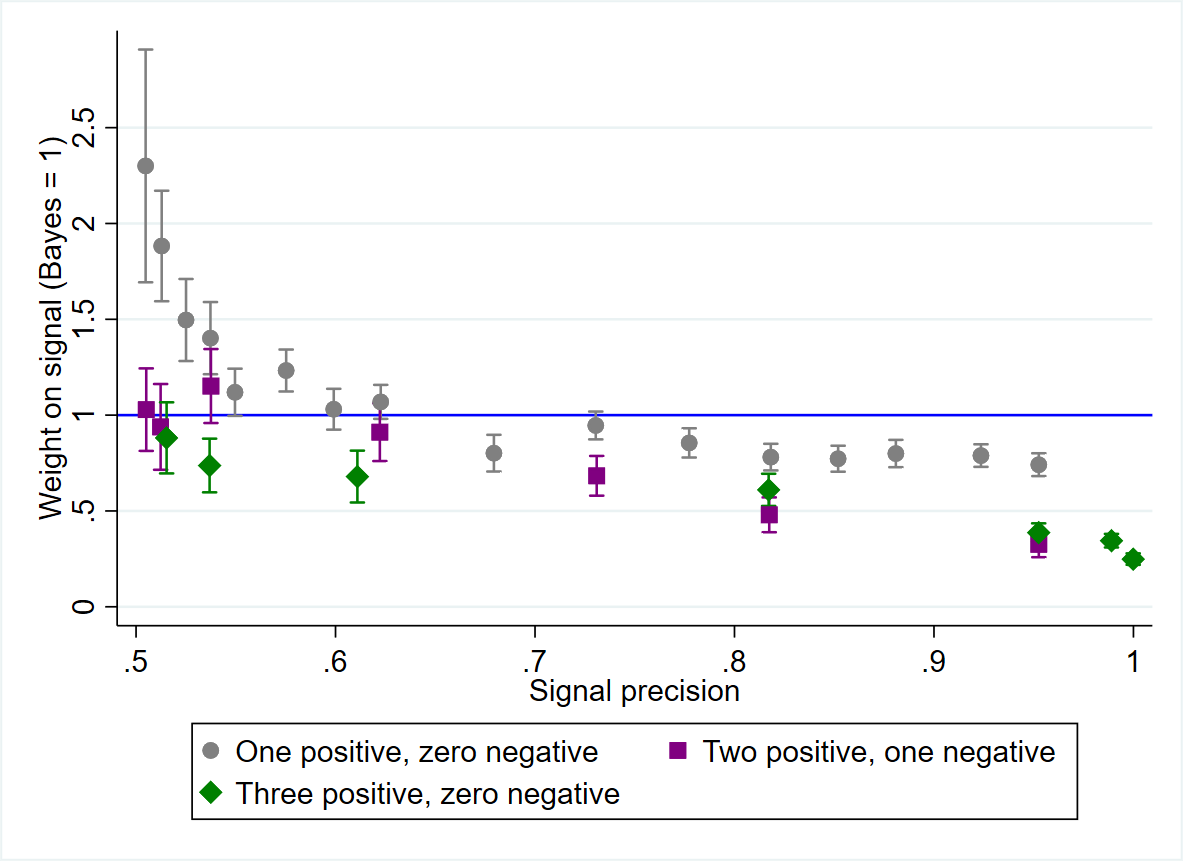
• Notes: This figure plots the average weight subjects put on signals relative to a Bayesian (indicated by the blue line), split by signal distribution. Grey circles correspond to one signal of strength $S$ (as in Figure 2); purple squares correspond to two signals of strength $S$ in one direction and one signal of strength $S$ in the opposing direction; green diamonds correspond to three signals of strength $S/3$ in the same the direction. This figure shows that subjects put less weight on three signals as compared to the weight they put on one signal. Error bars indicate 95% confidence intervals.

Figure A2: Over- and Underinference of Symmetric Signals by Signal Strength: Alternative Approach

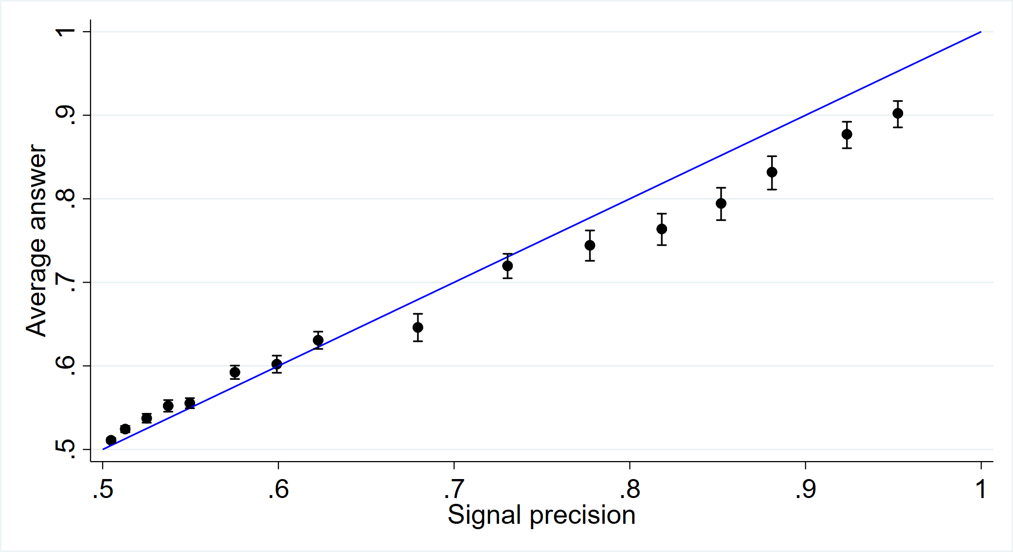
• Notes: This figure plots the average answer subjects give as a function of the Bayesian posterior. It differs from Figure 2 by first transforming subjects’ answers to be signal strengths, then averaging them, and then transforming back into precision estimates (as opposed to just averaging). The blue line indicates Bayesian behavior. The figure shows that subjects overweight weak signals and underweight strong signals. Error bars indicate 95% confidence intervals, clustered at the subject level.

Figure A3: Heterogeneity in Inference at the Individual Level

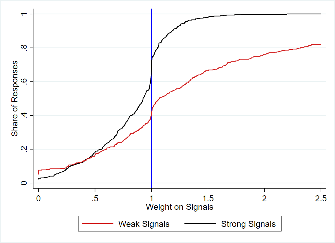
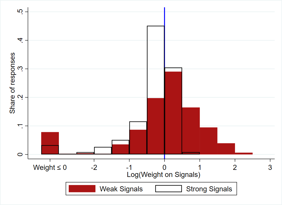
• Notes: This figure shows how much weight put on weak and strong signals at the individual level, where weight is defined relative to a Bayesian as in the main text. The top panel shows the CDF of individuals’ weights on strong and weak signals. The vertical line at 1 represents Bayesian updating. The bottom panel shows the PDF of the log of individuals’ weights on strong and weak signals. The vertical line at 0 represents Bayesian updating. Subjects with nonpositive weight are separated out. Weak signals have precision $p<0.6$ and strong signals have precision $p>0.7$. Observations are winsorized, for each signal strength, at the 5% level.

Figure A4: Heterogeneity in Inference from by News Consumption

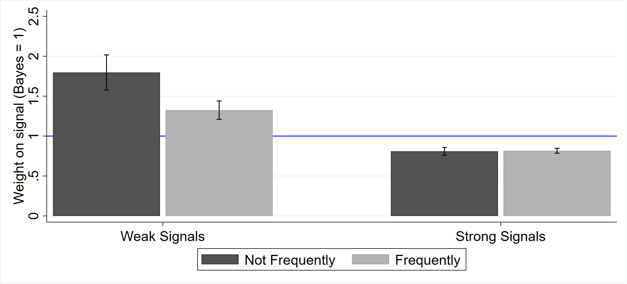
• Notes: The y-axis is weight subjects put on signals. Weak signals have precision between 0.5 and 0.6; strong signals have precision between 0.7 and 1. This figure plots weight by self-reported news consumption. Individuals who consume news “Never,” “Rarely,” or “Occasionally” are categorized as “Not Frequently.” Individuals who consume news “Somewhat Frequently,” “Frequently,” or “Very Frequently” are categorized as “Frequently.” This figure shows that news consumption is associated with less weight on weak signals and similar weight on strong signals. Error bars indicate 95% confidence intervals.

Figure A5: Movement and Uncertainty Reduction Over Time for Different Sports: 12 Time Chunks

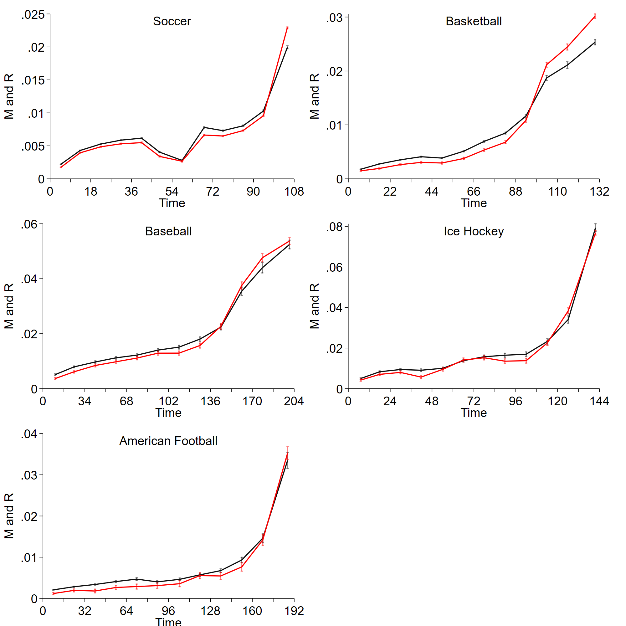
• Notes: This figure replicates Figure 6 with 36 time chunks.

Figure A6: Movement and Uncertainty Reduction Over Time for Finance Data: 12 Time Chunks

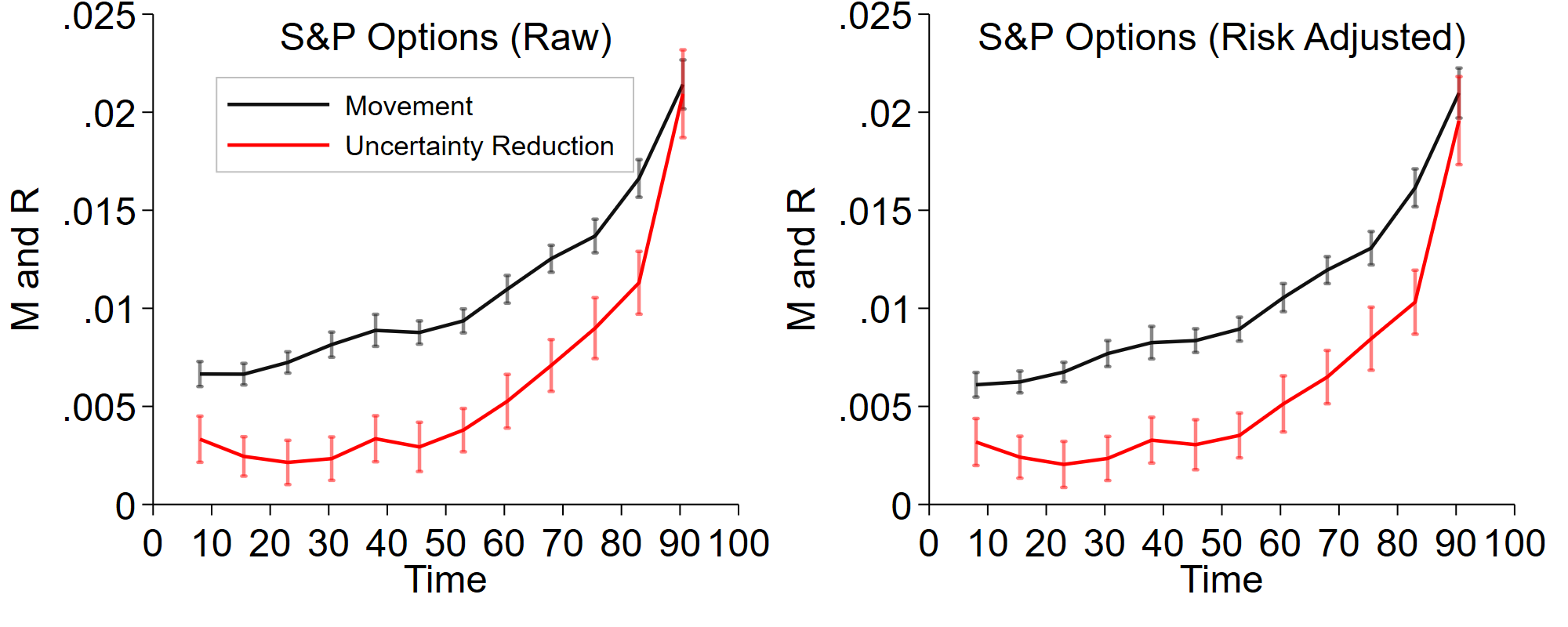
• Notes: This figure replicates Figure 7 with 12 time chunks.

Table A1: Regressions of Movement on Uncertainty Reduction: 12 Time Chunks

Dep Var:	Sports					Finance
Movement	Soccer	Basketball	Baseball	Hockey	Football	Raw	Risk-Adj.
Uncert. Red.	0.839	0.797	0.903	0.987	0.912	0.796	0.861
	(0.006)	(0.007)	(0.012)	(0.012)	(0.027)	(0.054)	(0.063)
Constant	0.0014	0.0018	0.0024	0.0013	0.0015	0.0060	0.0054
	(0.0003)	(0.0003)	(0.0004)	(0.0009)	(0.0002)	(0.0005)	(0.0005)
$R^{2}$	0.984	0.991	0.996	0.990	0.997	0.945	0.941
Time Chunks	12	12	12	12	12	12	12
Events	6,584	5,176	3,927	4,123	1,390	955	955
Observations	4,589,289	867,567	166,346	109,751	86,193	58,864	58,864
$p$-val.: $\beta_{1}=1$	<0.001	<0.001	<0.001	0.274	0.002	0.004	0.025
$p$-val.: $\beta_{0}=0$	<0.001	<0.001	<0.001	<0.001	<0.001	<0.001	<0.001

• Notes: This table replicates Table 2 with 12 time chunks.

Figure A7: Movement and Uncertainty Reduction Over Time for Different Sports: 36 Time Chunks

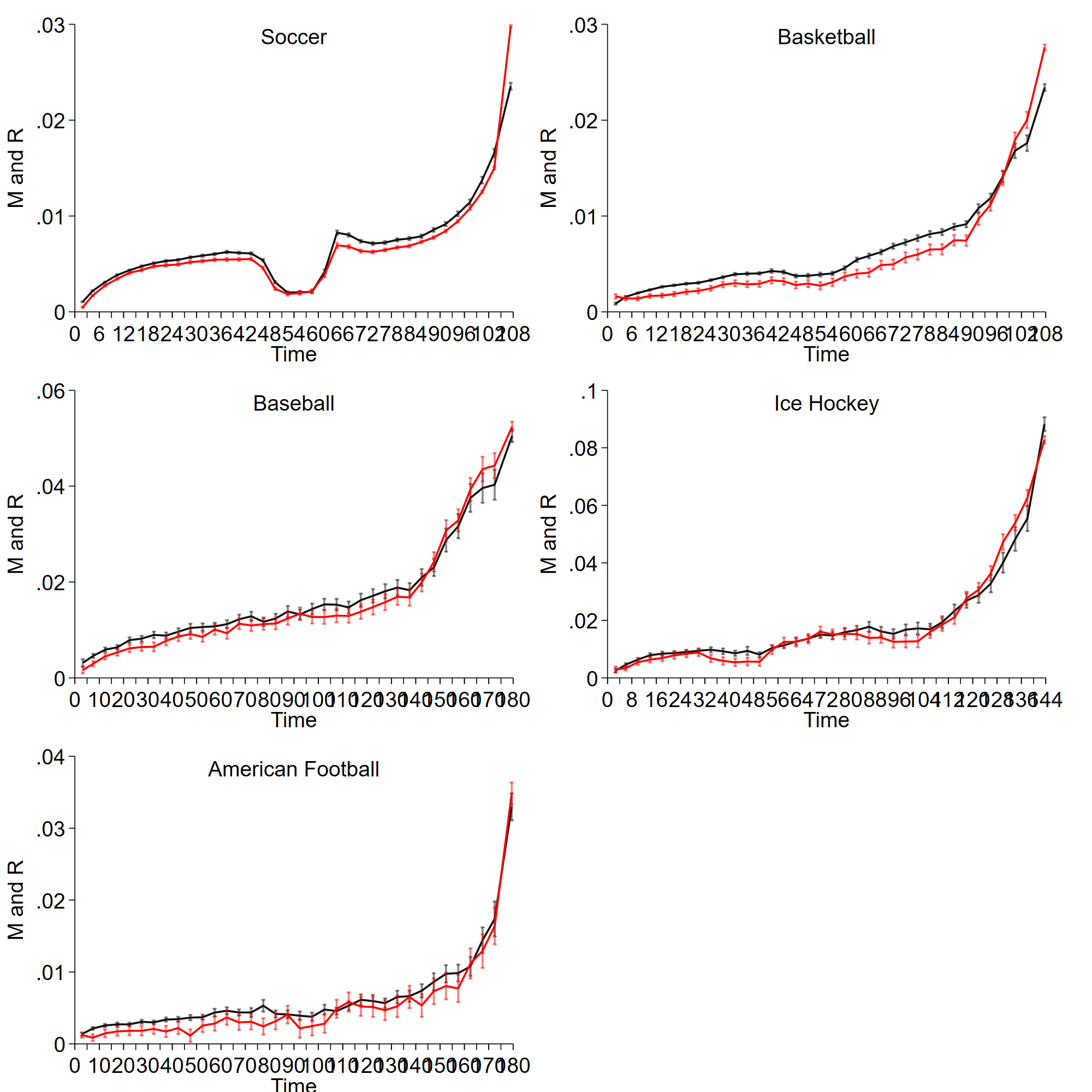
• Notes: This figure replicates Figure 6 with 36 time chunks.

Figure A8: Movement and Uncertainty Reduction Over Time for Finance Data: 36 Time Chunks

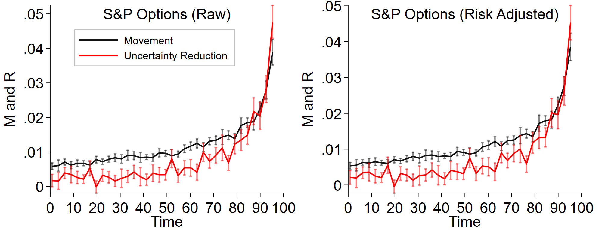
• Notes: This figure replicates Figure 7 with 36 time chunks.

Table A2: Regressions of Movement on Uncertainty Reduction: 36 Time Chunks

Dep Var:	Sports					Finance
Movement	Soccer	Basketball	Baseball	Hockey	Football	Raw	Risk-Adj.
Uncert. Red.	0.847	0.849	0.883	0.925	0.920	0.705	0.751
	(0.003)	(0.008)	(0.015)	(0.013)	(0.026)	(0.035)	(0.040)
Constant	0.0014	0.0016	0.0027	0.0020	0.0015	0.0063	0.0058
	(0.0001)	(0.0001)	(0.0002)	(0.0002)	(0.0001)	(0.0003)	(0.0003)
$R^{2}$	0.955	0.974	0.993	0.975	0.982	0.932	0.928
Time Chunks	36	36	36	36	36	36	36
Events	6,584	5,176	3,927	4,123	1,390	955	955
Observations	4,589,289	867,567	166,346	109,751	86,193	58,864	58,864
$p$-val.: $\beta_{1}=1$	<0.001	<0.001	<0.001	<0.001	0.054	<0.001	<0.001
$p$-val.: $\beta_{0}=0$	<0.001	<0.001	<0.001	<0.001	0.051	<0.001	<0.001

• Notes: This table replicates Table 2 with 36 time chunks.

Figure A9: Movement and Uncertainty Reduction for Options: Alternative Adjustments

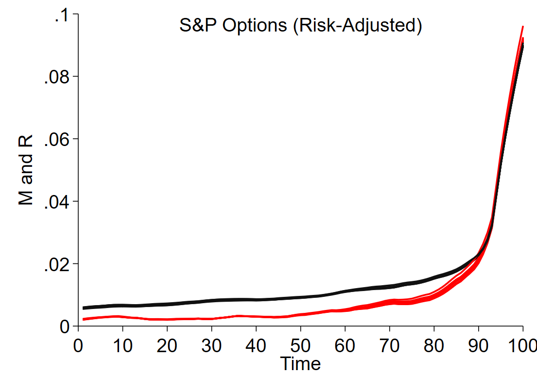
• Notes: This figure shows the smoothed average movement (black lines) and uncertainty reduction (red lines) statistics over time for the beliefs implied by option data (with 95% confidence intervals). Each line represents a different method to calculate risk-adjusted beliefs. While the different methods do lead to different inferred beliefs, the broad pattern of movement and uncertainty curves is very similar across the methods.

Appendix B Implementation Details for Finance Data

This Appendix describes our use of option-price data, as introduced in Section 5.4, in greater detail. First, we describe briefly how we translate from option prices to risk-neutral beliefs, and then we detail how we translate from risk-neutral to physical beliefs under different parameterizations for risk aversion.

B.1 Option Filters and the Risk-Neutral Distribution

Starting from the OptionMetrics data, we collect the same auxiliary data and take the same steps as described in full in Online Appendix C.5 of AL (2022) to measure the risk-neutral distribution for each date in our sample. First, we apply standard filters to the raw option-price data. We drop any options with bid or ask price of zero (or less than zero), with uncomputable Black–Scholes implied volatility or with implied volatility of greater than 100 percent, with more than one year to maturity, or (for call options) with mid prices greater than the price of the underlying; we drop any option cross-section (i.e., the full set of prices for the pair $(t,T)$) with no trading volume on date $t$, with fewer than three listed prices across different strikes, or for which there are fewer than three strikes for which both call and put prices are available (as is necessary to calculate the forward price and risk-free rate, which we calculate by applying the put-call parity relationship). We then measure the risk-neutral distribution following [53]: we translate the option mid-price quotes into implied volatilities; fit a clamped cubic spline to the implied volatility curve (with respect to the strike price) for each $(t,T)$ pair; transform these fitted implied volatilities back to prices; and then apply the usual [19] result to translate from prices to a risk-neutral distribution. Again see AL (2022) for full details.

B.2 Translating from Risk-Neutral to Physical Beliefs

We now describe the translation from risk-neutral to physical beliefs in greater detail. Assume there exists a representative investor (“the market”) with time-separable utility over the market index value. Assume, as above, that the state space (the set of possible terminal index values $V_{T}$) is discrete, with states indexed by $j$ ($V_{T}=\theta_{j}$ for $j=1,2,\ldots,J$), and denote terminal utility by $U(V_{T})$. The physical belief regarding the likelihood of state $j$ is $\pi_{t,j}$, and the risk-neutral belief is $\pi^{*}_{t,j}$. The two are related as follows:

$$\pi^{*}_{t,j}=\frac{U^{\prime}(\theta_{j})\pi_{t,j}}{\sum_{k}U^{\prime}(\theta_{k})\pi_{t,k}}.$$ (B1)

Our main translation assumes that $U^{\prime}(V_{T})=V_{T}^{-\gamma},$ corresponding to the assumption of power utility over the terminal index return, with constant relative risk aversion coefficient of $\gamma$. We then follow [16] in estimating $\gamma$ as the value under which the physical beliefs over the S&P 500 value at the one-month horizon are well calibrated (i.e., unbiased); see [16] for details on the maximum likelihood estimation procedure.

We then consider hundreds of generalizations of this basic framework. First, we reparameterize (B1) in terms of the ratio of marginal utilities (or SDF realizations) across adjacent index states $\phi_{j}$, by substituting $U^{\prime}(\theta_{j})=\phi_{j}U^{\prime}(\theta_{j-1})$. We then make a range of assumptions on the function $\phi_{j}$. We assume that $\phi_{j}$ varies by state $j$, either linearly or quadratically in $V_{T}$, and we estimate $\phi_{j}$ by maximum likelihood for each state; we assume that $\phi_{j}$ varies over time (either linearly or quadratically) or by horizon to expiration (as in [49]); and then we consider interactions in which $\phi_{j}$ varies both by bin $j$ and over time. In all cases (as can be seen in Figure A9, the right panel of which contains one line for each parameterization), the movement and uncertainty reduction statistics are close to unchanged. (This is in contrast to the physical probabilities, which do change depending on the parameterization; it is their evolution over time that is unchanged.)

Supplementary Appendix

Appendix C Experiment Study Materials

References

- [1] Hassan Afrouzi, Spencer Kwon, Augustin Landier, Yueran Ma and David Thesmar “Overreaction in Expectations: Evidence and Theory” In Working Paper, 2021
- [2] Sandro Ambuehl and Shengwu Li “Belief updating and the demand for information” In Games and Economic Behavior, 2018
- [3] George Marios Angeletos, Zhen Huo and Karthik A. Sastry “Imperfect macroeconomic expectations: Evidence and theory” In NBER Macroeconomics Annual 2020, 2021
- [4] Ned Augenblick and Eben Lazarus “A New Test of Excess Movement in Asset Prices” In Working Paper, 2022
- [5] Ned Augenblick and Matthew Rabin “Belief Movement, Uncertainty Reduction, and Rational Updating” In The Quarterly Journal of Economics, 2021
- [6] Yaron Azrieli, Christopher Chambers and Paul Healy “Incentives in Experiments: A Theoretical Analysis” In Journal of Political Economy, 2018
- [7] Cuimin Ba, J. Bohren and Alex Imas “Over- and Underreaction to Information” In Working Paper, 2022
- [8] Nicholas Barberis “Thirty years of prospect theory in economics: A review and assessment” In Journal of Economic Perspectives, 2013
- [9] Nicholas Barberis “Psychology-Based Models of Asset Prices and Trading Volume” In Chapter for the Handbook of Behavioral Economics, 2018
- [10] Lee Roy Beach, James Wise and Scott Barclay “Sample proportions and subjective probability revisions” In Organizational Behavior and Human Performance, 1970
- [11] Daniel Benjamin “Errors in Probabilistic Reasoning and Judgment Biases” In Chapter for the Handbook of Behavioral Economics, 2019
- [12] Daniel Benjamin, Don Moore and Matthew Rabin “Biased Beliefs about Random Samples: Evidence from Two Integrated Experiments” In Working Paper, 2018
- [13] Daniel Benjamin, Matthew Rabin and Collin Raymond “A Model of Nonbelief in the Law of Large Numbers” In Journal of the European Economic Association, 2016
- [14] Victor L. Bernard and Jacob K. Thomas “Post-Earnings-Announcement Drift: Delayed Price Response or Risk Premium?” In Journal of Accounting Research, 1989
- [15] Manudeep Bhuller and Henrik Sigstad “Do Judges Learn? The Causal Effects of Reversals on Judicial Decision-Making” In Working Paper, 2021
- [16] Robert R. Bliss and Nikolaus Panigirtzoglou “Option-Implied Risk Aversion Estimates” In Journal of Finance, 2004
- [17] Pedro Bordalo, Katherine Coffman, Nicola Gennaioli and Andrei Shleifer “Stereotypes” In Quarterly Journal of Economics, 2016
- [18] Pedro Bordalo, Nicola Gennaioli, Rafael La Porta and Andrei Shleifer “Belief Overreaction and Stock Market Puzzles” In Working Paper, 2022
- [19] Douglas T. Breeden and Robert H. Litzenberger “Prices of State-Contingent Claims Implicit in Option Prices” In Journal of Business, 1978
- [20] Alasdair Brown and Fuyu Yang “The wisdom of large and small crowds: Evidence from repeated natural experiments in sports betting” In International Journal of Forecasting, 2019
- [21] Martin Cripps “Divisible Updating” In Working Paper, 2018
- [22] Daniele d’Arienzo “Maturity increasing overreaction and bond market puzzles” In Working Paper, 2020
- [23] Chetan Dave and Katherine Wolfe “On confirmation bias and deviations from Bayesian updating” In Working Paper, 2003
- [24] Werner F.. De Bondt and Richard Thaler “Does the Stock Market Overreact?” In Journal of Finance, 1985
- [25] Michael Donnell and Wesley Du Charme “The effect of Bayesian feedback on learning in an odds estimation task” In Organizational Behavior and Human Performance, 1975
- [26] Ward Edwards “Conservatism in human information processing” In Formal Representation of Human Judgment (Ed: Kleinmuntz, B.) New York: Wiley, 1968
- [27] Benjamin Enke and Thomas Graeber “Cognitive Uncertainty” In Working Paper, 2023
- [28] Tony Fan, Yucheng Liang and Cameron Peng “Belief Updating: Inference versus Forecast Revision” In Working Paper, 2021
- [29] Gustav Fechner “Elements of Psychophysics” Breitkopf & Hartel (English translation: Holt, Rinehart,Winston, 1966)., 1860
- [30] Shane Frederick “Cognitive Reflection and Decision Making” In Journal of Economic Perspectives, 2005
- [31] Cary Frydman and Lawrence Jin “Efficient Coding and Risky Choice” In Working Paper, 2020
- [32] Stefano Giglio and Bryan Kelly “Excess Volatility: Beyond Discount Rates” In Quarterly Journal of Economics, 2018
- [33] Steven Gjerstad “Risk Aversion, Beliefs, and Prediction Market Equilibrium” In Working Paper, 2005
- [34] Russell Golman, George Loewenstein, Andras Molnar and Silvia Saccardo “The Demand for, and Avoidance of, Information” In Working Paper, 2021
- [35] Duarte Gonçalves, Jonathan Libgober and Jack Willis “Learning versus Unlearning: An Experiment on Retractions” In Working Paper, 2022
- [36] Paul Green, Michael Halbert and Patrick Robinson “An Experiment in Probability Estimation” In Journal of Marketing Research, 1965
- [37] David Grether “Bayes Rule as a Descriptive Model: The Representativeness Heuristic” In The Quarterly Journal of Economics, 1980
- [38] David Grether “Testing Bayes rule and the representativeness heuristic: Some experimental evidence” In Journal of Economic Behavior and Organization, 1992
- [39] Dale Griffin and Amos Tversky “The Weighing of Evidence and the Determinants of Confidence” In Cognitive Psychology, 1992
- [40] Neeraja Gupta, Luca Rigotti and Alistair Wilson “The Experimenters’ Dilemma: Inferential Preferences over Populations” In Working Paper, 2021
- [41] Charles Holt and Angela Smith “An update on Bayesian updating” In Journal of Economic Behavior and Organization, 2009
- [42] Tanjim Hossain and Ryo Okui “The binarized scoring rule” In The Review of Economic Studies, 2013
- [43] Daniel Kahneman and Amos Tversky “Prospect theory: An analysis of decision under risk” In Econometrica, 1979
- [44] Edna Kaufman, Miles Lord, Thomas Whelan Reese and John Volkman “The Discrimination of Visual Number” In The American Journal of Psychology, 1949
- [45] Mel Win Khaw, Ziang Li and Michael Woodford “Cognitive Imprecision and Small-Stakes Risk Aversion” In The Review of Economic Studies, 2021
- [46] Pascal Kieren, Jan Müller-Dethard and Martin Weber “Can Agents Add and Subtract When Forming Beliefs? Evidence from the Lab and Field” In Working Paper, 2022
- [47] Carlo Kraemer and Martin Weber “How Do People Take into Account Weight, Strength and Quality of Segregated vs. Aggregated Data? Experimental Evidence” In Journal of Risk and Uncertainty, 2004
- [48] Spencer Yongwook Kwon and Johnny Tang “Extreme Events and Overreaction to News” In Working Paper, 2022
- [49] Eben Lazarus “Horizon-Dependent Risk Pricing: Evidence from Short-Dated Options” In Working Paper, 2022
- [50] Steven Levitt and John A. List “What Do Laboratory Experiments Measuring Social Preferences Reveal About the Real World?” In Journal of Economic Perspectives, 2007
- [51] Yucheng Liang “Learning from Unknown Information Sources” In Working Paper, 2021
- [52] John A. List “Does Market Experience Eliminate Market Anomalies?” In Quarterly Journal of Economics, 2003
- [53] Allan M. Malz “A simple and reliable way to compute option-based risk-neutral distributions” In FRB of New York Staff Report 677, 2014
- [54] Charles F. Manski “Interpreting the predictions of prediction markets” In Economics Letters, 2006
- [55] Ian W.. Martin and Dimitris Papadimitriou “Sentiment and Speculation in a Market with Heterogeneous Beliefs” In American Economic Review, 2022
- [56] Cade Massey and George Wu “Detecting regime shifts: the causes of under- and overreaction” In Management Science, 2005
- [57] Marco Ottaviani and Peter Norman Sørensen “Price Reaction to Information with Heterogeneous Beliefs and Wealth Effects: Underreaction, Momentum, and Reversal” In American Economic Review, 2015
- [58] Cameron Peterson and Alan Miller “Sensitivity of subjective probability revision” In Journal of Experimental Psychology, 1965
- [59] Frederike Petzschner, Stefan Glasauer and Klaas Stephan “A Bayesian perspective on magnitude estimation” In Trends in Cognitive Sciences, 2015
- [60] Lawrence Phillips and Ward Edwards “Conservatism in a simple probability inference task” In Journal of Experimental Psychology, 1966
- [61] Shunichiro Sasaki and Toshiji Kawagoe “Belief Updating in Individual and Social Learning: A Field Experiment on the Internet” In Working Paper, 2007
- [62] Robert J. Shiller “Do Stock Prices Move Too Much to be Justified by Subsequent Changes in Dividends?” In American Economic Review, 1981
- [63] Stanley Smith Stevens “On the Theory of Scales of Measurement” In Science, 1946
- [64] Manoj Thomas and Vicki Morwitz “Penny Wise and Pound Foolish: The Left-Digit Effect in Price Cognition” In Journal of Consumer Research, 2005
- [65] Mattie Toma and Elizabeth Bell “Understanding and Improving Policymakers’ Sensitivity to Impact” In Working Paper, 2022
- [66] Amos Tversky and Daniel Kahneman “Advances in prospect theory: Cumulative representation of uncertainty” In Journal of Risk and Uncertainty, 1992
- [67] Emanuel Vespa and Alistair Wilson “Paired-Uniform Scoring: Implementing a Binarized Scoring Rule with Non-Mathematical Language” In Working Paper, 2017
- [68] Tuomo Vuolteenaho “What Drives Firm-Level Stock Returns?” In J. of Finance, 2002
- [69] Chen Wang “Under-and Overreaction in Yield Curve Expectations” In Working Paper, 2021
- [70] Justin Wolfers and Eric Zitzewitz “Interpreting prediction market prices as probabilities” In Working Paper, 2006
- [71] Michael Woodford “Modeling Imprecision in Perception, Valuation, and Choice” In Annual Review of Economics, 2020