Singularities and heteroclinic connections in complex-valued evolutionary equations with a quadratic nonlinearity
Abstract
In this paper, we consider the dynamics of solutions to complex-valued evolutionary partial differential equations (PDEs) and show existence of heteroclinic orbits from nontrivial equilibria to zero via computer-assisted proofs. We also show that the existence of unbounded solutions along unstable manifolds at the equilibrium follows from the existence of heteroclinic orbits. Our computer-assisted proof consists of three separate techniques of rigorous numerics: an enclosure of a local unstable manifold at the equilibria, a rigorous integration of PDEs, and a constructive validation of a trapping region around the zero equilibrium.
Keywords: nonlinear heat equation, heteroclinic connections, global existence of solution, rigorous numerics
1 Introduction
Understanding the long term behavior of solutions to evolutionary equations is fundamental to the discipline. This begins with questions of existence, and whether local existence can be extended globally. Of the solutions which exist globally, coherent structures (such as equilibria, traveling waves and periodic orbits) serve as emblematic examples of how solutions to a PDE may behave. The local stability of these coherent structures helps to inform us as to what type of phenomena are generically observable: while stable structures are robust and attract nearby trajectories, unstable objects repel solutions and are harder to detect. Nevertheless unstable objects are critically important in understanding the transient behavior of a system, and understanding to which particular stable state solutions will be attracted.
Characterizing the long term behavior of trajectories near an unstable object requires a global analysis, combining a perturbative analysis of solutions near the unstable object, with a non-perturbative analysis for when the solution is far from the invariant object. The non-perturbative analysis is genuinely difficult, and one often turns to numerical methods for insight. There are well established algorithms for integrating PDEs within a certain degree of precision. However in cases where the global existence of solutions is unknown, such as the 3D Navier-Stokes, it is not always obvious whether numerical results indicative of blowup are a genuine feature of the dynamics, or an artifact of the numerical method’s finite precision.
It is along these lines that we study the global dynamics and global wellposedness (or lack thereof) of the class of complex-valued nonlinear heat equations
| (1) |
under the periodic boundary condition in , where and . As a case study, we investigate trajectories on the unstable manifold of a nontrivial equilibrium of (1) at parameters . We numerically observe that most solutions are heteroclinic to the zero solution, however some solutions appear to grow without bound. By employing state-of-the-art techniques in validated numerics, we are able to rigorously characterize the limiting behavior of some solutions, and identify others where the numerical precision is lacking. Furthermore, through a forcing argument we can confirm the existence of unbounded solutions within the unstable manifold when .
Equation (1) can be seen as a generalization of a classical model for blowup in PDEs. When and the initial data is real, this reduces to the quadratic case of the Fujita equation on a bounded domain [Fuj66] whose blowup properties for non-negative initial data have been studied extensively [Lev90, DL00]. However as a complex equation the condition of non-negative real initial data is not an open property and finite time blowup, while present, does not occur as robustly [GNSY13]. By varying , we are able to compare the blowup phenomena and mechanisms between qualitatively disparate types of evolutionary equations. When then (1) is a nonlinear heat equation, when then (1) is a nonlinear Schrödinger equation, and for other values of the equation is similar to the complex Ginzburg-Landau equation.
Furthermore this equation arises from the mathematical studies by Masuda [Mas83, Mas84] and numerical observations by Cho et al. [COS16] to consider the nonlinear heat equation in the complex plane of time
| (2) |
on a straight path . This setting is slightly different from typical settings of complex-valued nonlinear heat equations, which often consider the complex-valued unknown function and both time and space variables are real-valued, see [GNSY13] for example. Our setting here is the case of nonlinear heat equations whose time variable is complex-valued.
As an innovative work, Masuda has considered the Cauchy problem of (2) under Neumann boundary conditions in [Mas83, Mas84]. He has proved global well-posedness of analytic solutions of (2) in a specific domain and existence of branching singularities at the movable singularity, which is called blow-up times in the case of real-valued nonlinear heat equations. Following Masuda’s studies, Cho et al. have numerically observed solution dynamics of the Cauchy problem of (2) under the periodic boundary condition in [COS16]. They have also presented that the solution may converge to the zero function on the straight path . This result agrees with Masda’s mathematical results in the case of the periodic boundary conditions.
Moreover, the present authors with H. Okamoto have studied the Cauchy problem of (2) under the same setting as Cho et al. [COS16] in [TLJO19] and have proved two results with computer-assistance. The first one is that there exists a branching singularity at the blow-up time, which extends the mathematical results by Masuda and mathematically proves numerical observations by Cho et al. The second one is global existence of the solution to the Cauchy problem of (1) for some . In particular, the initial data is given by , which is relatively large and far from a constant function. Therefore, this result agrees with Masuda’s work without the assumption of closeness to a constant. The proofs of these results are obtained by the tools of rigorous numerics such as rigorous integrator of time-dependent PDEs and numerical validation of center-stable manifolds. For further work using complexification to regularize singularities see [KSK17] and the references therein.
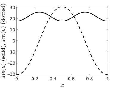
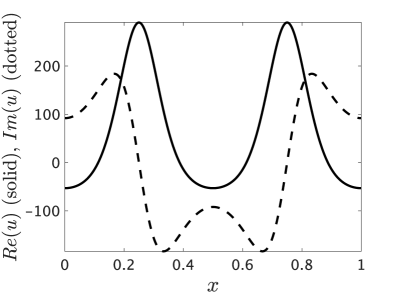
In contrast to the strictly real version of (2), the complex PDE in (1) possesses a diverse array of global solutions and a rich dynamical structure. In [JLT20] it was shown that when this equation has non-trivial complex-valued equilibria, whose profiles are shown in Figure 1. One may immediately see that the equilibria of (1) are independent of . In [JLT20] it was also shown that there exists an open set of homoclinic connections at the zero function, that is solutions which limit to the zero in both forward and backward time. Additionally in [Jaq21] it is shown that for , there are periodic orbits, and large monochromatic initial data which blows up in the norm.
Note also that since (1) has a nonlinearity of homogeneous degree then there exists a rescaling of solutions. That is, if solves (1) then
solves (1) as well. Hence the nontrivial equilibria proved to exist in [JLT20] in fact generate infinite families of equilibria of arbitrarily large norm. Furthermore, if there exists a heteroclinic orbit between the base nontrivial equilibria and the zero function, then it yields existence of a countable infinite number of heteroclinic orbits. This is in fact the case when .
Theorem 1.1 ([JLT20, Theorem 1.9]).
The heteroclinic orbit is obtained by combining three separate techniques of computer-assisted proofs: an enclosure of a local unstable manifold at the equilibria, a rigorous integration of the flow (starting from the unstable manifold) and a proof that the solution enters a validated stable set. The heteroclinic orbit is then obtained as a corollary, relying on the fact that when then (1) is a nonlinear Schrödinger equation, and moreover a reversible equation. In the case we would expect the heteroclinic orbit , although probably not , to persist.
In this paper, we perform a systematic study of the long term behavior of trajectories on the unstable manifold of the equilibrium in Figure 1 for . To focus our analysis we will restrict ourselves to studying a 1-complex dimensional submanifold. We will note however that while is unstable for all , its Morse index (that is the number of eigenvalues with positive real part), and hence the dimension of its unstable manifold does not stay constant as varies.
Indeed, for the equilibrium solution to (1), the eigenvalue problem is to find a pair such that
| (3) |
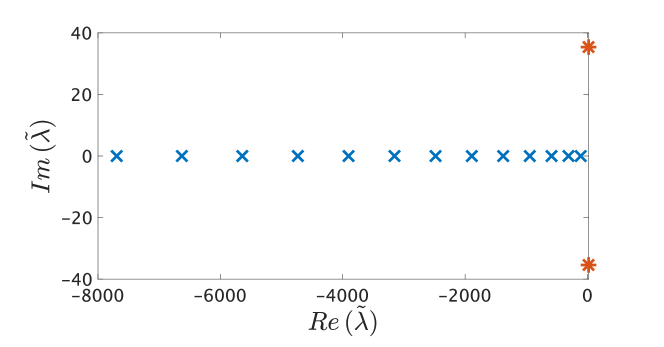
If there exists an eigenpair for , then will be an eigenpair for any and . For , we numerically calculate the eigenvalues with the largest real part to be:
| (4) | ||||
| (5) | ||||
| (6) | ||||
| (7) |
The rest of the eigenvalues appear to have zero imaginary part, see Figure 2, but this we cannot prove.
Given the rescaling of eigenvalues by the parameter and our calculation of the eigenvalues when , we can numerically determine the Morse index of the equilibrium. Then at some , there is one unstable eigenvalue, one purely imaginary eigenvalue, and infinitely many stable eigenvalues. Furthermore, for this equilibrium has two unstable eigenvalues, and for the equilibrium has only one unstable eigenvalue. Hence, for all the equilibrium will have an unstable manifold of complex dimension of or .
To restrict our analysis to something more tractable, we focus on the equilibrium shown in Figure 1. Then we will consider just the 1-complex dimensional unstable manifold of the equilibrium associated to the eigenvalue with the largest positive real part (sometimes called the strong unstable manifold). Let be an indexed parameter by integer . We will study solution behavior coming out of the 1-complex dimensional unstable manifold associated with the eigenpair . The index is taken from to so that we go around the manifold to investigate the solution behavior. Along this circular organization of the unstable manifold, we are able to show that many points will converge to zero. (These are just for particular angles. While the proof does extend to some open set about each angle, this is not the precise theorem we are stating here.) However for other angles we are not able to complete the proof. Below is what we can rigorously prove.
Remark 1.1.
Throughout the paper we work with a fixed eigenpair such that for all . This selection of eigenvalue corresponds with the lower red asterisk in Figure 2. For the choice of eigenvector , which in this case is neither unique in its phase nor its amplitude, we have fixed a particular choice in our code [JLT21].
Theorem 1.2.
Consider the nontrivial equilibrium to equation (1) and fix the eigenpair as described in Remark 1.1. For , let be a coordinate chart for a 1-complex dimensional submanifold of the unstable manifold.
-
(a)
For we prove that there exists a heteroclinic orbit from to (through the point ) for each integer degree angle except for the range .
-
(b)
For we prove that there exists a heteroclinic orbit from to (through the point ) for each integer degree angle except for the range .
-
(c)
For we prove that there exists a heteroclinic orbit from to (through the point ) for each integer degree angle except for the range .
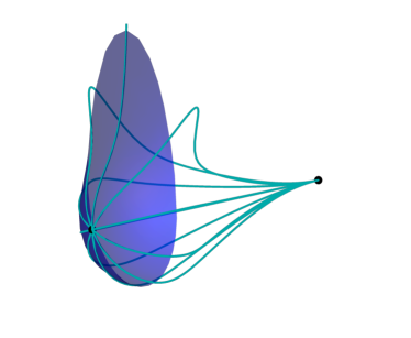
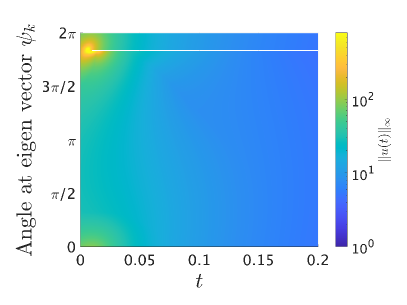
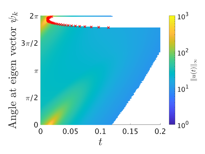
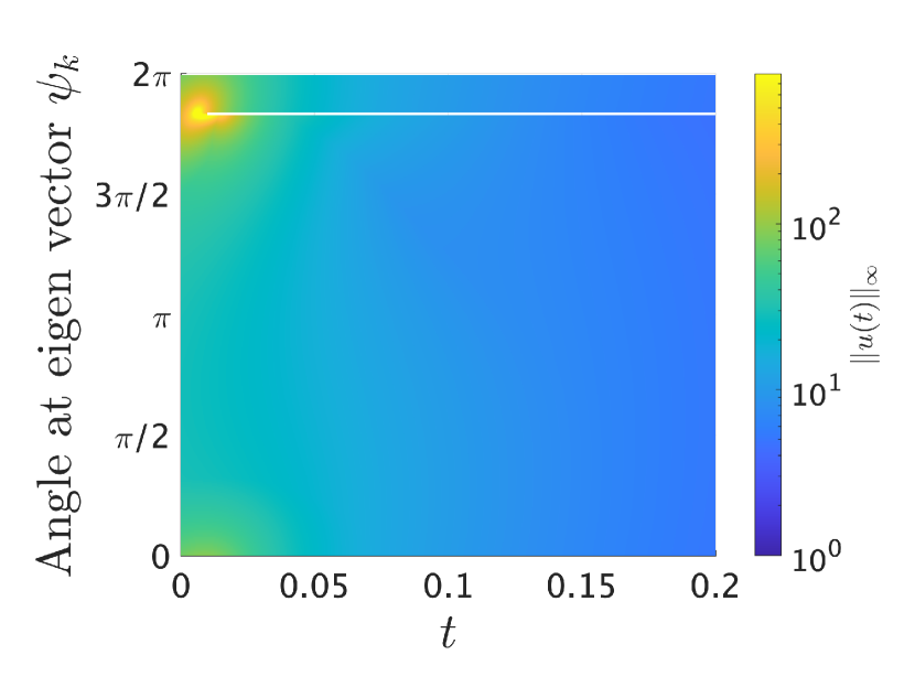
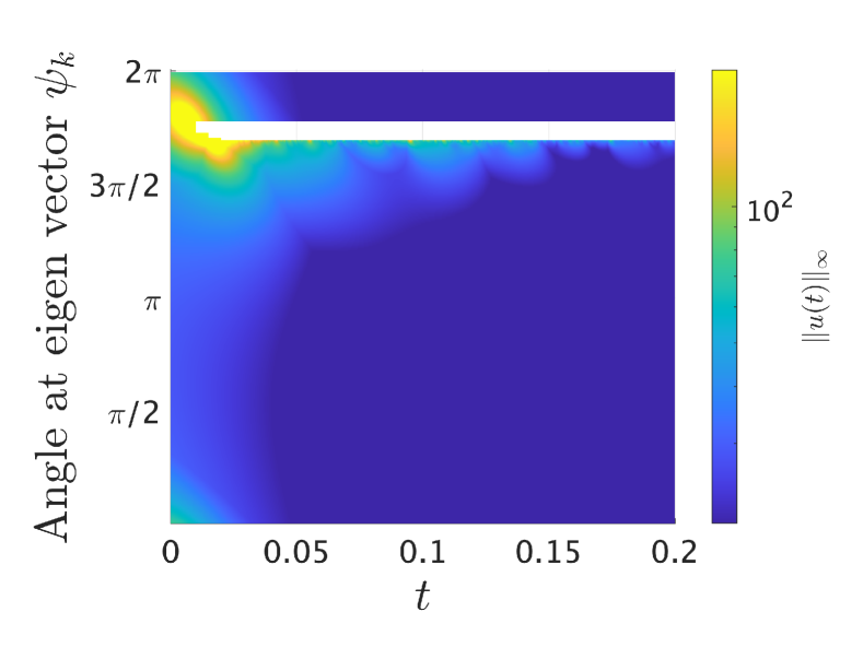
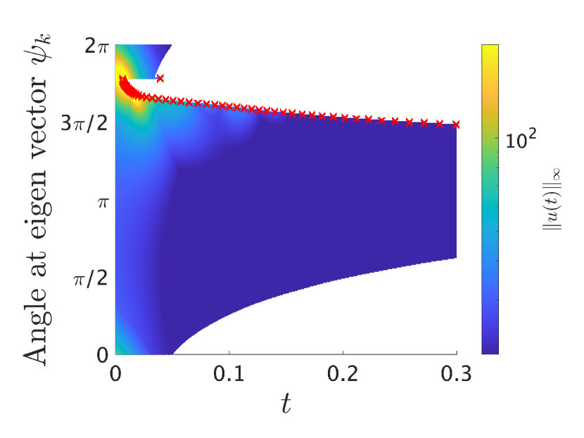
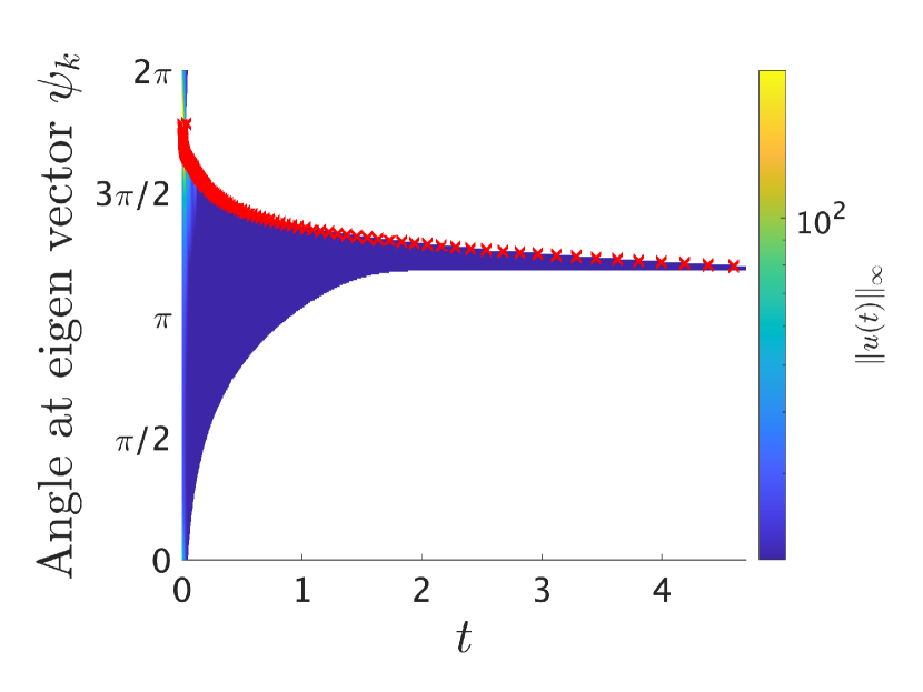
For angles at which we are unable to obtain a computer-assisted proof (CAP), the long term behavior of the solution is unclear. One possibility is that the solution will eventually converge to zero, however the precision of our computation was insufficient to produce a CAP. Another possibility is that the solution will grow without bound, either in finite time (a blowup solution) or in infinite time (a growup solution). We suspect the angles where our CAP fails to form a neighborhood about a growup/blowup solution, see Figure 3. For example, in our purely numerical calculations at our non-rigorous integrator failed at only a single angle . Furthermore, solutions on either side of this non-proof interval display qualitatively different behavior suggestive of a branching singularity, see Figure 4. We note that our CAP approach succeeded in proving non-trivial solution behaviors for the angle , whose amplitude is significantly large.
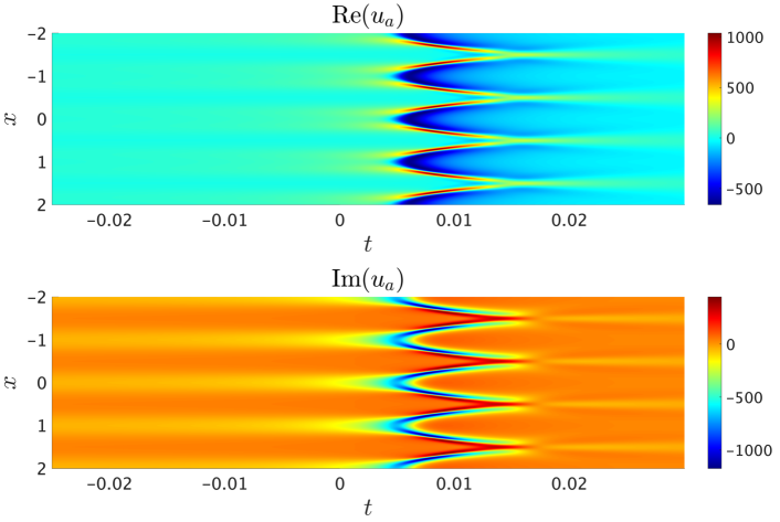
() A part of heteroclinic connection from to at the angle with .
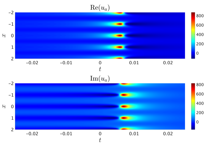
() A part of heteroclinic connection from to at the angle with .
By using validated numerics we are able to be notified of the possible existence of singularities that would otherwise be subtle to detect. If we had used a coarser resolution of angles in our calculation of Figure 3 (right) we may have missed the single angle where our non-rigorous numerics break down. (In fact for our non-rigorous computations did not breakdown for any of the angles .) While evidence of a branching singularity can still be found in a faint discontinuity in the graph of (as and are varied), it is a subtle matter to verify. In contrast, by using validated numerics we are readily alerted to a possible singularity. However with the present methods it is unclear how to distinguish between an isolated singularity, and singularities occurring on a very small interval of .
Furthermore, when we are able to prove the existence of unbounded solutions.
Theorem 1.3.
Consider the non-trivial equilibrium for (1). Let . There exists a point in the unstable manifold of through which the solution is unbounded in positive time.
This proof closely mimics a result obtained in [Stu18] and relies on the fact that the nonlinearity in (1) is holomorphic and (1) generates an analytic semigroup when . We conjecture that the nonlinear Schrödinger equation () also has solutions that are unbounded. Note also that this theorem does not distinguish between finite time blowup and infinite time growup.
The rest of the paper is organized as follows: In the following three sections, we briefly show three separate fundamental techniques of computer-assisted proofs. These have been introduced in previous studies [TLJO19, JLT20], and some minor modifications are made for the current problem. In Section 2 we introduce the parameterization method for 1-complex dimensional unstable manifolds of equilibrium to (1). Section 3 is devoted to introducing a method of rigorous integration of PDEs in forward time. Section 4 is an introduction of constructing a trapping region near the zero equilibrium. Finally, we conclude in Section 5, where we present the proof of our main theorems (Theorems 1.2 and 1.3), and conclude with discussions and outlook of the present study.
2 Parameterization of the Local Unstable Manifold
As mentioned already in the Introduction, the proof of Theorem 1.2 relies on a rigorous parameterization of the unstable manifold of a steady state (see Figure 1) of the nonlinear equation (1). Note that satisfies . Solutions of (1) with periodic boundary conditions may be expanded in Fourier series as
| (8) |
and matching like terms, this leads to the infinite system of nonlinear ODEs
| (9) |
where , which denotes the discrete convolution. As in [JLT20], we assume that the Fourier coefficients in (8) satisfy the symmetry
| (10) |
From the symmetry assumption, one only needs to solve for the non-negative Fourier coefficients. Let so that (9) can be more densely written as . Denote by the Fourier coefficients of the steady state (already proven in [JLT20]), that is
By construction, since is an equilibrium, its Fourier coefficients satisfy .
Denote the unstable manifold of the steady states by
Consider the solution of the linearized problem (3) (as described in Remark 1.1) such that the real part of the eigenvalue is positive. Under these assumptions, we introduce the theory to parameterize 1-complex dimensional unstable manifolds of steady states of the nonlinear equation (1). The approach is based on the Parameterization Method (e.g. see [CFdlL03a, CFdlL03b, CFdlL05]) for unstable manifolds, and follows closely the presentation of [RMJ19].
We are interested in solutions of (9) whose spectral representation have geometrically decaying Fourier coefficients. Given an geometric decay rate , this feature is encapsulated in the weighted Banach algebra
| (11) |
Indeed, given two sequences , with their discrete convolution given component-wise by
| (12) |
one has that .
Denote by the Fourier coefficients of the eigenvector (which solves (3)), that is
The Fourier eigenpair satisfies , which becomes, in the space of Fourier coefficients
Note that for and , we assume that the symmetry condition (10) holds. The (computer-assisted) approach to obtain the steady state and the eigenpair is already obtained and presented in [RMJ19].
Denote by the closed unit disk centered at in the complex plane.
Given an angle , we look for a function satisfying the invariance equation
| (13) |
for all subject to the first order constraints
| (14) |
If solves (13) subject to the first order constraints (14), then one can easily verify that for every , the function
| (15) |
solves the differential equation on given by on . Moreover, since and , then parameterizes a subset of the unstable manifold for given by
| (16) |
We call the set in (16) the local unstable manifold at associated to in the direction . Note that is a sub-manifold of the unstable manifold .
The strategy is now clear: compute a function which solves (13) subject to the first order constraints given in (14). We represent as a power series
| (17) |
The coefficients of the power series (17) are elements of the Banach space
| (18) |
Define the Taylor-Fourier product as follows: given ,
| (19) |
where is the standard discrete convolution (12). One can verify that is a Banach algebra, that is given ,
| (20) |
Plugging the power series (17) in the invariance equation (13) and imposing the first order constraints (14) leads to look for a solution of , where the map is given by
| (21) |
The following result shows that a zero of provides the Fourier-Taylor coefficients of the expansion of a parameterization of the local unstable manifold at associated to in the direction .
Lemma 2.1.
Let and suppose that solves . For each , denote . Then, for each ,
The previous result paves the way to come, that is to prove the existence of such that . This is done using the following Newton-Kantorovich type theorem, which we now introduce. Before that, denote by the closed ball of radius centered at .
Theorem 2.2 (A Newton-Kantorovich type theorem).
Let be a bounded linear operator (typically an approximate inverse of ). Consider a point (typically a numerical approximation), assume that is injective and that . Let be a nonnegative constant, and a function satisfying
| (22) | ||||
| (23) |
where denotes the operator norm. Define the radii polynomial by
| (24) |
If there exists such that , then there exists a unique such that .
Since the construction of the bounds and satisfying (22) and (23), respectively, is almost exactly the same as the ones presented in [JLT20], we omit their construction here.
In practice, the rigorous computation of , the local unstable manifold at associated to in the direction is done as follows. Starting with the Fourier coefficients of the steady state and the eigenpair , we consider a finite dimensional reduction of defined in (21) on which we apply Newton’s method to obtain a numerical approximation , yielding a Fourier-Taylor coefficients of the approximation
| (25) |
We wrote a MATLAB program (available at [JLT21]) which rigorously computes (i.e. controlling the floating point errors) the bounds and as presented in Theorem 2.2. The program uses the interval arithmetic library INTLAB available at [Rum99]. Fixing and using the MATLAB program, the code verifies the existence of such that . By Theorem 2.2, there exists a unique such that . By construction, the resulting function given by
parameterizes the local unstable manifold at associated to in the direction . Moreover, for each , . We get the rigorous error bound
We applied this approach to obtain the parameterizations of for the values . As pointed out already in [JLT20] (see Remark 3.3), the continuity of the bounds and in the parameter implies that if the computer-assisted proof is performed for , then, there exists such that , and hence, the unique solution of satisfies . This in turn implies that for each , and therefore the corresponding points on are analytic in space.
3 Rigorous Integrator
In this section we briefly introduce a method of rigorous numerical integration for (1) in forward time. This is firstly proposed in [TLJO19] and then slightly improved for integrating the solution of the nonlinear Schrödinger (NLS) case () in [JLT20]. For proving the existence of heteroclinic orbits for (1), this integrator will propagate the rigorous inclusion of 1-complex dimensional unstable manifold , which is given by the parameterization method described in Section 2.
Let us assume that the initial data is presented by the Fourier series
where is the same sequence space as in the previous section, but the definition of its norm is slightly changed as because there is no need to assume the symmetry (10) in the followings. Under the Fourier ansatz of defined in (8), we consider the Cauchy problem of (9) with the initial data . For a fixed time , let be a time step. The Banach space in which we validate rigorously the local existence of the solution is defined by
Let be a truncated approximation of with the Fourier projection . We rigorously include the solution of (9) in a neighborhood of defined by
To represent the ODEs (9) more densely, we define the Laplacian operator acting on as
and denotes the domain of the operator . For let us define
| (26) |
Then we consider the ODEs (9) as the zero-finding problem . That is, if with the initial condition holds, such solves the Cauchy problem of (9). We also define an operator as
| (27) |
where is the evolution operator (cf., e.g.,[Paz83]) on . Such evolution operator is defined by a solution map of the linearized problem of (9) at ,
| (28) |
with any initial data (). In other words, the evolution operator provides the solution of (28) via the relation . In [TLJO19, Theorem 3.2], we give a hypothesis to validate existence of the evolution operator. Checking the hypothesis by using rigorous numerics, we also provide a uniform bound of the evolution operator over the simplex , that is a computable constant satisfying
| (29) |
Such a constant is obtained by solving the linearized problem (28) via decomposing the solution by the finite mode and the tail for satisfying .
The rigorous integrator we used for proving heteroclinic orbits is based on the following theorem, which provides the local existence (in time) of the solution via interval techniques.
Theorem 3.1 ([TLJO19, Theorem 4.1]).
Given the approximate solution of (9) and the initial sequence , assume that holds for . Assume also that, for any , holds, where is given by
| (30) |
Here, and satisfy and , respectively. If there exists such that
then the exact Fourier coefficients of the solution of (9) are rigorously included in and are unique in .
The proof of Theorem 3.1 is based on Banach’s fixed-point theorem for the operator defined in (27). For more details, we refer to our previous papers [TLJO19, Section 4] for the case of and [JLT20, Section 4] for .
We applied this theorem iteratively to extend the local inclusion of the solution over longer time intervals. Let be grid points in time. We call the time step. Let us also define () with the stepsize of , which can be changed adaptively. Firstly, we assume that the solution of (9) is rigorously included in , where denotes an approximate solution given in . Secondly, we set the next time step in order to obtain the uniform bound of evolution operator . Thirdly, the initial data is updated by the endpoint of solution on , that is . Replacing , we apply Theorem 3.1 for the Cauchy problem on . We validate the sufficient condition of Theorem 3.1 and then obtain the next inclusion . Finally, go back to the second step and repeat these processes several times. Thus, we can extend the local inclusion of solution until the sufficient condition of Theorem 3.1 is no longer satisfied. This time stepping scheme works successfully for the complex-valued nonlinear heat equations with the cases .
To complete the proof of existence of heteroclinic orbits, we need to prove the global existence of the solution after the numerical verification of the local inclusion using the time stepping. We construct a trapping region near the zero equilibrium, which guarantees the global existence of solution converging to zero. The next section is devoted to introducing how we construct such a trapping region rigorously.
4 Trapping Region
If the zero equilibrium to (1) was linearly stable then it would be relatively straightforward to construct a trapping region, that is an open set within which every initial condition will converge to the zero equilibrium in forward time. However this is not the case. Indeed, from (9) one sees that the linearized flow has eigenvalues for all . For all there exists a single zero eigenvalue, which presents a significant obstacle in identifying a trapping region.
The eigenspace associated with the zero eigenvalue corresponds to spatially constant solutions, and naturally forms an invariant subspace of the nonlinear dynamics. The dynamics on this subspace are governed by the ordinary differential equation , whose solutions with initial condition may be explicitly given by below
| (31) |
Geometrically, these solutions foliate the origin by homoclinic orbits, with the exception of initial conditions which blowup in finite positive/negative time.
While the center manifold associated with the zero eigenvalue contains solutions which blowup in finite time, an open set of initial conditions solutions will converge to zero with monotonically decreasing norm. To that end we make the following definition.
Definition 4.1.
For any define the region
| (32) |
To then develop a trapping region about the zero equilibrium, we will restrict to initial data whose zeroth Fourier coefficients are contained in some region . When then all of the other eigenvalues in the linearization have negative real part. In [TLJO19], we characterized an explicit trapping region about the zero equilibrium using a Lyapunov-Perron argument to demonstrate a stable foliation of the region . However this analysis depended on the eigenvalues having a negative real part, and could not be extended to the case .
Treating the NLS case (where all eigenvalues lie on the imaginary axis) requires a different approach. In [JLT20] a theorem was proved which identifies a trapping region about the zero equilibrium, by blowing up the dynamics about the spatially homogeneous solutions. This approach does not take advantage of any exponential decay in the higher Fourier modes, as it was constructed to treat the NLS case where no such decay is present. However in the case where the trapping region argument in [JLT20] can be readily adapted, as the exponential decay in the higher Fourier modes only assists in the analysis.
Let denote the inclusion into the 0th Fourier mode. Below we present the trapping region theorem from [JLT20] adapted for the case when one is integrating in the complex plane of time. The proof is trivially different, and is left to the reader.
Theorem 4.2 (cf [JLT20] Theorem 2.3).
In short, if parameters are such that the inequality (34) is satisfied, then is a trapping region. As the left-hand side of (34) is monotonically increasing in and , it is ideal to take these parameters as small as possible. For an explicit sequence , one may readily compute values of , for which , and then search for a value of for which (34) is satisfied. A similar procedure may be done when considering a ball about , and we refer to [JLT20] for further details.
5 Results and discussions
Finally, combining the above three techniques, namely the parameterization of the local unstable manifold (Section 2), the rigorous integrator (Section 3) and the computation of the trapping region (Section 4), we present the proofs of our main theorems. The proof of Theorem 1.2 is completed with computer assistance. All the codes for generating the following results with computer-assisted proofs are available at [JLT21].
5.1 Proof of Theorem 1.2 and 1.3
Proof of Theorem 1.2.
Our proof of existence of heteroclinic orbits consist of three parts. Firstly we construct the parameterization of the strong unstable manifold associated with the eigenpair introduced in Section 2. Secondly rigorous integrator provided in Section 3 starts from the rigorous inclusion of the endpoint of unstable manifold. The integrator propagates the inclusion of a point on the unstable manifold in forward time using the time stepping scheme. Finally, we validate that the hypothesis of Theorem 4.2 holds after several time stepping, that is the solution of the Cauchy problem enters the trapping region described in Section 4. Then the whole orbit connects the equilibrium to zero. This completes the proof.
(a) For , our computer-assisted approach succeeded in proving the heteroclinic orbits with indices . The results of validation are shown in Figure 5 (right). We have almost the same solution distribution as the one given by non-rigorous numerics. For indices , Our computer-assisted approach failed to prove the global existence of solution (in the third step). There are two reasons for such failure. One is that the propagation of errors causes the validation to fail. This is a limitation of the rigorous integrator. Further improvements of the integrator are needed to better control the propagation of errors. The other is that the asymptotic to an unbounded solution makes it impossible to validate the global existence of solutions. As presented in Figure 3, the solution profile appears to blowup for some angles. Since our proof is based on rigorous numerics, we have strong evidence of existence of blow-up solutions.
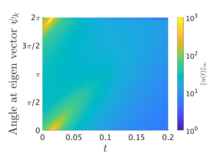
(b) We show the results for the case of in Figure 6 (right). As in the case of , the distribution of solutions is almost the same as the one obtained by non-rigorous numerics. Our computer-assisted approach succeeded in proving existence of heteroclininc orbits except for the indices , which is slightly narrower compared with the case of . This is because the amplitude of the solution profiles is smaller than that for . The main difference from the case of is that the Morse index of the equilibrium is different (2 for and 1 for ). Other than that, the results of computer-assisted proofs were almost the same as the case. We also have an evidence to conjecture that there could be blow-up solutions for some angles.
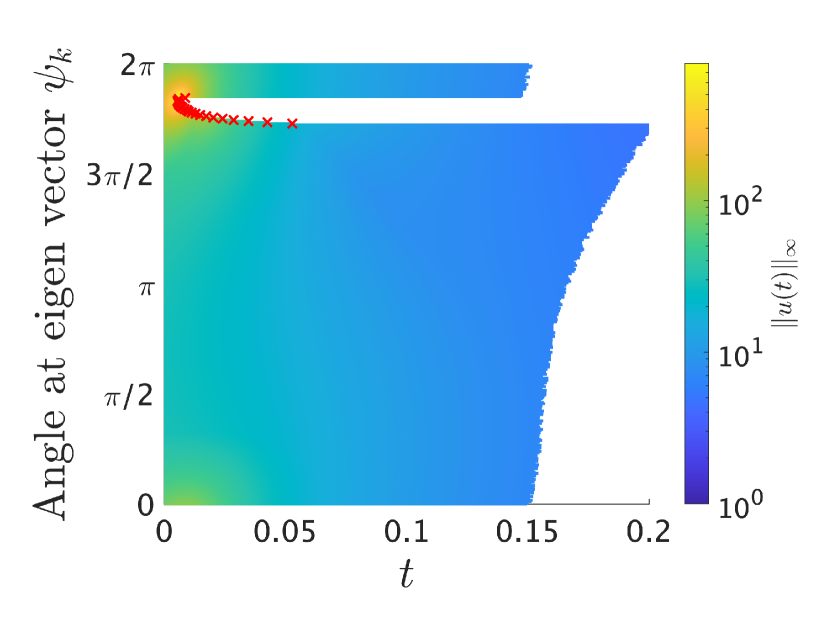
(c) Finally, for (the nonlinear Schrödinger case), Figure 7 (b) and (c) show results of our computer-assisted proofs. In this case the nontrivial equilibrium has one unstable eigenvalue, one stable eigenvalue, and infinitely many imaginary eigenvalues. Therefore it is easy to predict that the dynamics of the solution is different from the cases . Compared to the other two cases, the behavior of the solution is more complicated, which is shown in Figure 7 (a). The former solution appears to be transitioning smoothly, while the latter solution appears to be more oscillatory. Then such oscillatory behaving solution is difficult to validate, and failed in the range . More precisely, the error propagation is so significant that it is difficult to integrate the solution rigorously (see Figure 7 (c)). However, our results, as in the other two cases, suggest that there could be a blowup of solutions at certain angles. ∎
(a)
(b)
(c)
Proof of Theorem 1.3.
The proof follows from virtually the same argument as given in [Stu18, Lemma 2.6], which we summarize below.
For and the unit disk , let denote a parameterization of the strong unstable manifold about the equilibrium given in Theorem 1.2. By the construction, as described in Section 2, the map is analytic. Fix a continuous linear functional which separates and , whereby and is analytic.
Consider the flow map of the evolutionary equation (1). If then is an analytic semigroup. For we define a sequence of projected time- maps given by
As this is a composition of analytic functions, each is analytic.
The proof of unbounded solutions proceeds by contradiction. Suppose there is a uniform bound such that for all . By the construction of our parameterization , we have for all . As we have demonstrated with computer-assisted proofs at parameters , there exists a heteroclinic point such that and , the zero equilibrium. As the trapping region constructed in Theorem 4.2 is an open set, then there exists a neighborhood about such that all points in are heteroclinic points between and . Hence for all . Recall that as separates and , then .
Since the functions are uniformly bounded, by the Vitali theorem there exists an analytic function to which the sequence converges uniformly on compact subsets. As argued above, for all . As is analytic and locally constant on the open set , then must be constant and equal on all of . But this contradicts . Thus the functions cannot be uniformly bounded for all . As was chosen to be an arbitrary continuous linear functional which separates and , it follows that the globalization of the strong unstable manifold of must be unbounded.
∎
Theorem 1.3 establishes the existence of solutions which limit to the non-trivial equilibrium in negative time, and are unbounded in positive time. However it does not distinguish whether such a solution exists for all time, a so-called growup solution, or blows up in finite time. Note also that Theorem 1.3 is stated just for , because we cite Theorem 1.2 for the existence of a heteroclinic orbit. For other values of the existence of an heteroclinic orbit from to similarly would force the existence of unbounded solutions. However this argument does not readily extend to the case . This is because when then (1) becomes a nonlinear Schrödinger equation, and the flow map generates a continuous semigroup, but not an analytic semigroup.
5.2 Discussion and Outlook
Numerics are often indispensable in understanding nonlinear evolutionary equations. However the reliability of these techniques are significantly affected when trajectories are integrated for a long time or their norm becomes very large. This is necessarily the case when studying unstable manifolds or blowup solutions, so it is important to know how much we can trust numerics in these situations.
In this work, we have investigated the long term behavior of solutions in the (1-complex dimensional) strong unstable manifold of a nontrivial equilibrium . By considering the equation (1) for the parameters we are able to investigate how our numerical technique behave in the dissipative regime, the dispersive regime, and in between.
By using rigorous numerics, we are able to answer questions that are not typically accessible by standard numerical methods. Namely we are able to rigorously establish that the finite precision with which we performed our computations was sufficient to prove the existence of heteroclinic orbits from to . Hence additional calculations at higher precision are not necessary for us to be confident of our result. And by using a forcing argument from complex analysis, we are able to establish the existence of unbounded solutions which limit to in negative time.
The restriction to only considering the strong unstable manifold of provides a tractable restriction for us to focus our analysis. This isolates the primary difficulties of long integration time, and solutions which pass near a singularity. However as mentioned in Section 1, for the unstable manifold of has complex dimension two. Thus our restriction to the strong unstable manifold is not capturing all of the dynamics in the entire unstable manifold. Not to mention that equation (1) has infinitely other equilibria which we have not studied in this paper.
Nevertheless, the entire picture of how all of the dynamics behave on these strong unstable manifolds is still incomplete. Somewhat generalizing the open question in [JLT20], we make the following conjecture.
Conjecture 5.1.
For all there exists a unique trajectory in the (1-complex dimensional) strong unstable manifold of which blows up in finite time.
It could be feasible to extend our current techniques used to prove Theorem 1.2 by a parameter continuation in , and prove that there is a heteroclinic orbit from to for all . By the same argument in Theorem 1.3 this would force the existence of unbounded solutions which limit to in backwards time, for all . However it still remains to prove the existence of unbounded solutions in the NLS case of .
Furthermore our current proof of unbounded solutions does not establish finite time blowup. In the case we proved in [TLJO19] that the initial data blows up at time using rigorous numerics. This argument followed the approach of Masuda, wherein we integrated the solution in the complex plane of time to establish a branching singularity. Such an approach could be directly applied to prove blowup for other initial data, but only if the blowup set is robust and not isolated. In finite dimensional ODEs the recent work [LMT21] has demonstrated computer-assisted proofs of unstable blowup. However it is unclear how to extend this technique to the infinite dimensional case.
Acknowledgements
The second author was supported by an NSERC Discovery Grant. The third author was supported by JSPS KAKENHI Grant Numbers JP18K13453, JP20H01820, JP21H01001.
References
- [CFdlL03a] X. Cabré, E. Fontich, and R. de la Llave. The parameterization method for invariant manifolds. I. Manifolds associated to non-resonant subspaces. Indiana Univ. Math. J., 52(2):283–328, 2003.
- [CFdlL03b] X. Cabré, E. Fontich, and R. de la Llave. The parameterization method for invariant manifolds. II. Regularity with respect to parameters. Indiana Univ. Math. J., 52(2):329–360, 2003.
- [CFdlL05] X. Cabré, E. Fontich, and R. de la Llave. The parameterization method for invariant manifolds. III. Overview and applications. J. Differential Equations, 218(2):444–515, 2005.
- [COS16] C.-H. Cho, H. Okamoto, and M. Shōji. A blow-up problem for a nonlinear heat equation in the complex plane of time. Japan Journal of Industrial and Applied Mathematics, 33(1):145–166, Feb 2016.
- [DL00] Keng Deng and Howard A Levine. The role of critical exponents in blow-up theorems: the sequel. Journal of Mathematical Analysis and Applications, 243(1):85–126, 2000.
- [Fuj66] Hiroshi Fujita. On the blowing up of solutions of the Cauchy problem for . J. Fac. Sci. Univ. Tokyo Sect. I, 13:109–124 (1966), 1966.
- [GNSY13] Jong-Shenq Guo, Hirokazu Ninomiya, Masahiko Shimojo, and Eiji Yanagida. Convergence and blow-up of solutions for a complex-valued heat equation with a quadratic nonlinearity. Trans. Amer. Math. Soc., 365:2447–2467, 2013.
- [Jaq21] Jonathan Jaquette. Quasiperiodicity and blowup in integrable subsystems of nonconservative nonlinear Schrödinger equations. arXiv preprint arXiv:2108.00307, 2021.
- [JLT20] Jonathan Jaquette, Jean-Philippe Lessard, and Akitoshi Takayasu. Global dynamics in nonconservative nonlinear Schrödinger equations. arXiv preprint arXiv:2012.09734, 2020.
- [JLT21] Jonathan Jaquette, Jean-Philippe Lessard, and Akitoshi Takayasu. Codes of “Singularities and heteroclinic connections in complex-valued evolutionary equations with a quadratic nonlinearity”. https://github.com/taklab-org/Singularities-heteroclinic-connections-cveeqs, 2021.
- [KSK17] Panayotis G Kevrekidis, Constantinos I Siettos, and Yannis G Kevrekidis. To infinity and some glimpses of beyond. Nature communications, 8(1):1–13, 2017.
- [Lev90] Howard A Levine. The role of critical exponents in blowup theorems. Siam Review, 32(2):262–288, 1990.
- [LMT21] Jean-Philippe Lessard, Kaname Matsue, and Akitoshi Takayasu. A geometric characterization of unstable blow-up solutions with computer-assisted proof. arXiv preprint arXiv:2103.12390, 2021.
- [Mas83] Kyûya Masuda. Blow-up of solutions of some nonlinear diffusion equations. In Hiroshi Fujita, Peter D. Lax, and Gilbert Strang, editors, Nonlinear Partial Differential Equations in Applied Science; Proceedings of The U.S.-Japan Seminar, Tokyo, 1982, volume 81 of North-Holland Mathematics Studies, pages 119 – 131. North-Holland, 1983.
- [Mas84] Kyûya Masuda. Analytic solutions of some nonlinear diffusion equations. Mathematische Zeitschrift, 187(1):61–73, Mar 1984.
- [Paz83] A. Pazy. Semigroups of Linear Operators and Applications to Partial Differential Equations. Applied mathematical sciences. Springer, 1983.
- [RMJ19] Christian Reinhardt and J. D. Mireles James. Fourier-Taylor parameterization of unstable manifolds for parabolic partial differential equations: formalism, implementation and rigorous validation. Indag. Math. (N.S.), 30(1):39–80, 2019.
- [Rum99] S.M. Rump. INTLAB - INTerval LABoratory. In Tibor Csendes, editor, Developments in Reliable Computing, pages 77–104. Kluwer Academic Publishers, Dordrecht, 1999. http://www.ti3.tu-harburg.de/rump/.
- [Stu18] Hannes Stuke. Complex time blow-up of the nonlinear heat equation. 2018.
- [TLJO19] Akitoshi Takayasu, Jean-Philippe Lessard, Jonathan Jaquette, and Hisashi Okamoto. Rigorous numerics for nonlinear heat equations in the complex plane of time. arXiv preprint arXiv:1910.12472, 2019.