Deep Reinforcement Learning at the Edge of the Statistical Precipice
Abstract
Deep reinforcement learning (RL) algorithms are predominantly evaluated by comparing their relative performance on a large suite of tasks. Most published results on deep RL benchmarks compare point estimates of aggregate performance such as mean and median scores across tasks, ignoring the statistical uncertainty implied by the use of a finite number of training runs. Beginning with the Arcade Learning Environment (ALE), the shift towards computationally-demanding benchmarks has led to the practice of evaluating only a small number of runs per task, exacerbating the statistical uncertainty in point estimates. In this paper, we argue that reliable evaluation in the few-run deep RL regime cannot ignore the uncertainty in results without running the risk of slowing down progress in the field. We illustrate this point using a case study on the Atari 100k benchmark, where we find substantial discrepancies between conclusions drawn from point estimates alone versus a more thorough statistical analysis. With the aim of increasing the field’s confidence in reported results with a handful of runs, we advocate for reporting interval estimates of aggregate performance and propose performance profiles to account for the variability in results, as well as present more robust and efficient aggregate metrics, such as interquartile mean scores, to achieve small uncertainty in results. Using such statistical tools, we scrutinize performance evaluations of existing algorithms on other widely used RL benchmarks including the ALE, Procgen, and the DeepMind Control Suite, again revealing discrepancies in prior comparisons. Our findings call for a change in how we evaluate performance in deep RL, for which we present a more rigorous evaluation methodology, accompanied with an open-source library rliable111https://github.com/google-research/rliable, to prevent unreliable results from stagnating the field.
1 Introduction
Research in artificial intelligence, and particularly deep reinforcement learning (RL), relies on evaluating aggregate performance on a diverse suite of tasks to assess progress. Quantitative evaluation on a suite of tasks, such as Atari games [5], reveals strengths and limitations of methods while simultaneously guiding researchers towards methods with promising results. Performance of RL algorithms is usually summarized with a point estimate of task performance measure, such as mean and median performance across tasks, aggregated over independent training runs.
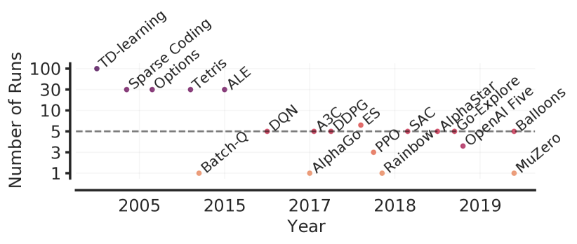
A small number of training runs (Figure 1) coupled with high variability in performance of deep RL algorithms [41, 70, 17, 16, 68], often leads to substantial statistical uncertainty in reported point estimates. While evaluating more runs per task has been prescribed to reduce uncertainty and obtain reliable estimates [41, 20, 49], 3-10 runs are prevalent in deep RL as it is often computationally prohibitive to evaluate more runs. For example, 5 runs each on 50+ Atari 2600 games in ALE using standard protocol requires more than 1000 GPU training days [15]. As we move towards more challenging and complex RL benchmarks (e.g., StarCraft [110]), evaluating more than a handful of runs will become increasingly demanding due to increased amount of compute and data needed to tackle such tasks. Additional confounding factors, such as exploration in the low-data regime, exacerbates the performance variability in deep RL – as seen on the Atari 100k benchmark [50] – often requiring many more runs to achieve negligible statistical uncertainty in reported estimates.
Ignoring the statistical uncertainty in deep RL results gives a false impression of fast scientific progress in the field. It inevitably evades the question: “Would similar findings be obtained with new independent runs under different random conditions?” This could steer researchers towards superficially beneficial methods [11, 25, 12], often at the expense of better methods being neglected or even rejected early [74, 67] as such methods fail to outperform inferior methods simply due to less favorable random conditions. Furthermore, only reporting point estimates obscures nuances in comparisons [85] and can erroneously lead the field to conclude which methods are state-of-the-art [63, 84], ensuing wasted effort when applied in practice [108]. Moreover, not reporting the uncertainty in deep RL results makes them difficult to reproduce except under the exact same random conditions, which could lead to a reproducibility crisis similar to the one that plagues other fields [44, 78, 4]. Finally, unreliable results could erode trust in deep RL research itself [45].
In this work, we show that recent deep RL papers compare unreliable point estimates, which are dominated by statistical uncertainty, as well as exploit non-standard evaluation protocols, using a case study on Atari 100k (Section 3). Then, we illustrate how to reliably evaluate performance with only a handful of runs using a more rigorous evaluation methodology that accounts for uncertainty in results (Section 4). To exemplify the necessity of such methodology, we scrutinize performance evaluations of existing algorithms on widely used benchmarks, including the ALE [5] (Atari 100k, Atari 200M), Procgen [18] and DeepMind Control Suite [104], again revealing discrepancies in prior comparisons (Section 5). Our findings call for a change in how we evaluate performance in deep RL, for which we present a better methodology to prevent unreliable results from stagnating the field.
How do we reliably evaluate performance on deep RL benchmarks with only a handful of runs? As a practical solution that is easily applicable with 3-10 runs per task, we identify three statistical tools (Table 1) for improving the quality of experimental reporting. Since any performance estimate based on a finite number of runs is a random variable, we argue that it should be treated as such. Specifically, we argue for reporting aggregate performance measures using interval estimates via stratified bootstrap confidence intervals, as opposed to point estimates. Among prevalent aggregate measures, mean can be easily dominated by performance on a few outlier tasks, while median has high variability and zero performance on nearly half of the tasks does not change it. To address these deficiencies, we present more efficient and robust alternatives, such as interquartile mean, which are not unduly affected by outliers and have small uncertainty even with a handful of runs. Furthermore, to reveal the variability in performance across tasks, we propose reporting performance distributions across all runs. Compared to prior work [5, 83], these distributions result in performance profiles [26] that are statistically unbiased, more robust to outliers, and require fewer runs for smaller uncertainty.
| Desideratum | Current Evaluation Protocol | Our Recommendation |
|---|---|---|
| Uncertainty in aggregate performance | Point estimates • Ignore statistical uncertainty • Hinder results reproducibility | Interval estimates via stratified bootstrap confidence intervals |
| Variability in performance across tasks and runs | Tables with mean scores per task • Overwhelming beyond a few tasks • Standard deviations often omitted • Incomplete picture for multimodal and heavy-tailed distributions | Performance profiles (score distributions) • Show tail distribution of scores on combined runs across tasks • Allow qualitative comparisons • Easily read any score percentile |
| Aggregate metrics for summarizing performance across tasks | Mean • Often dominated by performance on outlier tasks Median • Requires large number of runs to claim improvements • Poor indicator of overall performance: zero scores on nearly half the tasks do not affect it | Interquartile Mean (IQM) across all runs • Performance on middle 50% of combined runs • Robust to outlier scores but more statistically efficient than median To show other aspects of performance gains, report average probability of improvement and optimality gap. |
2 Formalism
We consider the setting in which a reinforcement learning algorithm is evaluated on tasks. For each of these tasks, we perform independent runs222A run can be different from using a fixed random seed. Indeed, fixing the seed may not be able to control all sources of randomness such as non-determinism of ML frameworks with GPUs (e.g., Figure A.13). which each provide a scalar, normalized score , and . These normalized scores are obtained by linearly rescaling per-task scores333Often the average undiscounted return obtained during an episode (see Sutton and Barto [101] for an explanation of the reinforcement learning setting). based on two reference points; for example, performance on the Atari games is typically normalized with respect to a random agent and an average human, who are assigned a normalized score of 0 and 1 respectively [75]. We denote the set of normalized scores by .
In most experiments, there is inherent randomness in the scores obtained from different runs. This randomness can arise from stochasticity in the task, exploratory choices made during learning, randomized initial parameters, but also software and hardware considerations such as non-determinism in GPUs and in machine learning frameworks [116]. Thus, we model the algorithm’s normalized score on the task as a real-valued random variable . Then, the score is a realization of the random variable , which is identically distributed as . For , we define the tail distribution function of as . For any collection of scores , the empirical tail distribution function is given by . In particular, we write .
The aggregate performance of an algorithm maps the set of normalized scores to a scalar value. Two prevalent aggregate performance metrics are the mean and median normalized scores. If we denote by the average score on task across runs, then these aggregate metrics are and . More precisely, we call these sample mean and sample median over the task means since they are computed from a finite set of runs. Since is a realization of the random variable , the sample mean and median scores are point estimates of the random variables and respectively. We call true mean and true median the metrics that would be obtained if we had unlimited experimental capacity (), given by and respectively.
Confidence intervals (CIs) for a finite-sample score can be interpreted as an estimate of plausible values for the true score. A CI computes an interval such that if we rerun the experiment and construct the CI using a different set of runs, the fraction of calculated CIs (which would differ for each set of runs) that contain the true score would tend towards , where is the nominal coverage rate. 95% CIs are typically used in practice. If the true score lies outside the 95% CI, then a sampling event has occurred which had a probability of 5% of happening by chance.
Remark. Following Amrhein et al. [2], Wasserstein et al. [112], Romer [87], we recommend using confidence intervals for measuring the uncertainty in results and showing effect sizes (e.g., performance improvements over baseline) that are compatible with the given data. Furthermore, we emphasize using statistical thinking but avoid statistical significance tests (e.g., -value < ) because of their dichotomous nature (significant vs. not significant) and common misinterpretations [35, 33, 73] such as 1) lack of statistically significant results does not demonstrate the absence of effect (Figure 2, right), and 2) given enough data, any trivial effect can be statistically significant but may not be practically significant.
3 Case Study: The Atari 100k benchmark
We begin with a case study to illustrate the pitfalls arising from the naïve use of point estimates in the few-run regime. Our case study concerns the Atari 100k benchmark [50], an offshoot of the ALE for evaluating data-efficiency in deep RL. In this benchmark, algorithms are evaluated on only 100k steps (2-3 hours of game-play) for each of its 26 games, versus 200M frames in the ALE benchmark. Prior reported results on this benchmark have been computed mostly from 3 [55, 39, 59, 72, 89, 95] or 5 runs [50, 107, 53, 51, 86, 115, 64, 54, 66], and more rarely, 10 [93, 65] or 20 runs [56].
Our case study compares the performance of five recent deep RL algorithms, namely: (1) der [107] and (2) otr [51], (3) drq444drq codebase uses non-standard evaluation hyperparameters. Instead, drq corresponds to drq with standard -greedy parameters [14, Table 1] in ALE. See Appendix for more details. [53], (4) curl [56], and (5) spr [93]. We chose these methods as representative of influential algorithms within this benchmark. Since good performance on one game can result in unduly high sample means without providing much information about performance on other games, it is common to measure performance on Atari 100k using sample medians. Refer to Appendix A.2 for more details about the experimental setup.
We investigate statistical variations in the few-run regime by evaluating 100 independent runs for each algorithm, where the score for a run is the average returns obtained in 100 evaluation episodes taking place after training. Each run corresponds to training one algorithm on each of the 26 games in Atari 100k. This provides us with scores per algorithm, which we then subsample with replacement to 3–100 runs. The subsampled scores are then used to produce a collection of point estimates whose statistical variability can be measured. We begin by using this experimental protocol to highlight statistical concerns regarding median normalized scores.
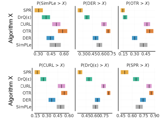
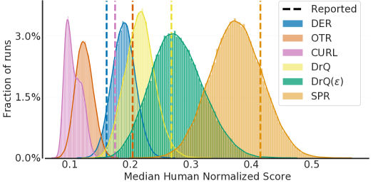
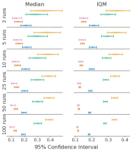
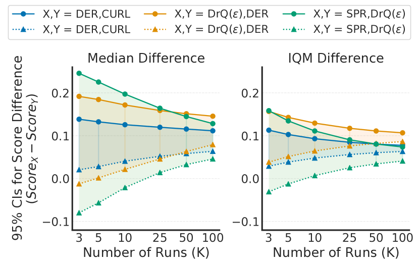
High variability in reported results. Our first observation is that the sample medians reported in the literature exhibit substantial variability when viewed as random quantities that depend on a small number of sample runs (Figure 2, left). This shows that there is a fairly large potential for drawing erroneous conclusions based on point estimates alone. As a concrete example, our analysis suggests that der may in fact be better than otr, unlike what the reported point estimates suggest. We conclude that in the few-run regime, point estimates are unlikely to provide definitive answers to the question: “Would we draw the same conclusions were we to re-evaluate our algorithm with a different set of runs?”

Substantial bias in sample medians. The sample median is a biased estimator of the true median: in general. In the few-run regime, we find that this bias can dominate the comparison between algorithms, as evidenced in Figure 3. For example, the score difference between sample medians with 5 and 100 runs for spr (+0.03 points) is about 36% of its mean improvement over drq (+0.08 points). Adding to the issue, the magnitude and sign of this bias strongly depends on the algorithm being evaluated.
Statistical concerns cannot be satisfactorily addressed with few runs. While claiming improvements with 3 or fewer runs may naturally raise eyebrows, folk wisdom in experimental RL suggests that 20 or 30 runs are enough. By calculating 95% confidence interval555Specifically, we use the bootstrap [9] to calculate the interval between percentiles of the distribution of sample medians (95% CIs). on sample medians for a varying number of runs (Figure 2, right), we find that this number is closer to 50–100 runs in Atari 100k – far too many to be computationally feasible for most research projects.
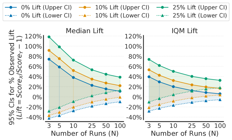
Consider a setting in which an algorithm is known to be better – what is the reliability of median and IQM (Section 4.3) for accurately assessing performance differences as the number of runs varies? Specifically, we consider two identical -run experiments involving spr, except that we artificially inflate one of the experiments’ scores by a fixed fraction or lift of (Figure 6). In particular, corresponds to running the same experiment twice but with different runs. We find that statistically defensible improvements with median scores is only achieved for 25 runs () and 100 runs (). With , even 100 runs are insufficient, with deviations of possible.
Changes in evaluation protocols invalidates comparisons to prior work. A typical and relatively safe approach for measuring the performance of an RL algorithm is to average the scores received in their final training episodes [69]. However, the field has seen a number of alternative protocols used, including reporting the maximum evaluation score achieved during training [75, 1, 3] or across multiple runs [47, 32, 82]. A similar protocol is also used by curl and sunrise [59] (Appendix A.4).
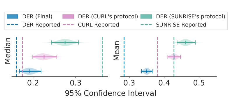
Results produced under alternative protocols involving maximum are generally incomparable with end-performance reported results. On Atari 100k, we find that the two protocols produce substantially different results (Figure 6), of a magnitude greater than the actual difference in score. In particular, evaluating der with curl’s protocol results in scores far above those reported for curl. In other words, this gap in evaluation procedures resulted in curl being assessed as achieving a greater true median than der, where our experiment gives strong support to der being superior. Similarly, we find that a lot of sunrise’s improvement over der can be explained by the change in evaluation protocol (Figure 6). Refer to Appendix A.4 for discussion on pitfalls of such alternative protocols.
4 Recommendations and Tools for Reliable Evaluation
Our case study shows that the increase in the number of runs required to address the statistical uncertainty issues is typically infeasible for computationally demanding deep RL benchmarks. In this section, we identify three tools for improving the quality of experimental reporting in the few-run regime, all aligned with the principle of accounting for statistical uncertainty in results.
4.1 Stratified Bootstrap Confidence Intervals
We first reaffirm the importance of reporting interval estimates to indicate the range within which an algorithm’s aggregate performance is believed to lie. Concretely, we propose using bootstrap CIs [29] with stratified sampling for aggregate performance, a method that can be applied to small sample sizes and is better justified than reporting sample standard deviations in this context. While prior work has recommended using bootstrap CIs for reporting uncertainty in single task mean scores with runs [41, 16, 20], this is less useful when is small (Figure A.18), as bootstrapping assumes that re-sampling from the data approximates sampling from the true distribution. We can do better by aggregating samples across tasks, for a total of random samples.
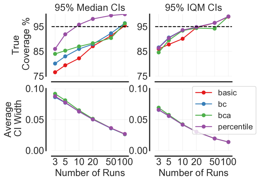
To compute the stratified bootstrap CIs, we re-sample runs with replacement independently for each task to construct an empirical bootstrap sample with runs each for tasks from which we calculate a statistic and repeat this process many times to approximate the sampling distribution of the statistic. We measure the reliability of this technique in Atari 100k for variable , by comparing the nominal coverage of 95% to the “true” coverage from the estimated CIs (Figure 6) for different bootstrap methods (see [30] and Appendix A.5). We find that percentile CIs provide good interval estimates for as few as runs for both median and IQM scores (Section 4.3).
4.2 Performance Profiles
Most deep RL benchmarks yield scores that vary widely between tasks and may be heavy-tailed, multimodal, or possess outliers (e.g., Figure A.14). In this regime, both point estimates, such as mean and median scores, and interval estimates of these quantities paint an incomplete picture of an algorithm’s performance [24, Section 3]. Instead, we recommend the use of performance profiles [26], commonly used in benchmarking optimization software. While performance profiles from Dolan and Moré [26] correspond to empirical cumulative distribution functions without any uncertainty estimates, profiles proposed herein visualize the empirical tail distribution function (Section 2) of a random score (higher curve is better), with pointwise confidence bands based on stratified bootstrap.
By representing the entire set of normalized scores visually, performance profiles reveal performance variability across tasks much better than interval estimates of aggregate metrics. Although tables containing per-task mean scores and standard deviations can reveal this variability, such tables tend to be overwhelming for more than a few tasks.666In addition, standard deviations are sometimes omitted from tables due to space constraints. In addition, performance profiles are robust to outlier runs and insensitive to small changes in performance across all tasks [26].
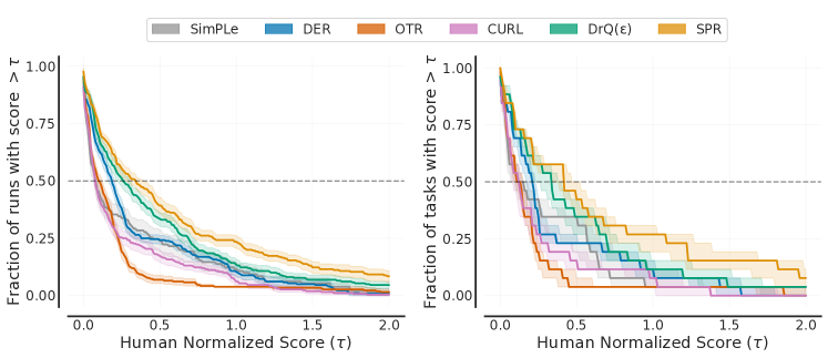
In this paper, we propose the use of a performance profile we call run-score distributions or simply score distributions (Figure 7, right), particularly well-suited to the few-run regime. A score distribution shows the fraction of runs above a certain normalized score and is given by
| (1) |
One advantage of the score distribution is that it is an unbiased estimator of the underlying distribution . Another advantage is that an outlier run with extremely high score can change the output of score distribution for any by at most a value of .
It is useful to contrast score distributions to average-score distributions, originally proposed in the context of the ALE [5] as a generalization of the median score. Average-score distributions correspond to the performance profile of a random variable , , which shows the fraction of tasks on which an algorithm performs better than a certain score. However, such distributions are a biased estimate of the thing they seek to represent. Run-score distributions are more robust than average-score distributions, as they are a step function in versus intervals, and typically has less variance: versus . Figure 7 illustrates these differences.
4.3 Robust and Efficient Aggregate Metrics
Performance profiles allow us to compare different methods at a glance. If one curve is strictly above another, the better method is said to stochastically dominate777A random variable has stochastic dominance over random variable if for all , and for some , . the other [61, 27]. In RL benchmarks with a large number of tasks, however, stochastic dominance is rarely observed: performance profiles often intersect at multiple points. Finer quantitative comparisons must therefore entail aggregate metrics.
We can extract a number of aggregate metrics from score distributions, including median (mixing runs and tasks) and mean normalized scores (matching our usual definition). As we already argued that these metrics are deficient, we now consider interesting alternatives also derived from score distributions.
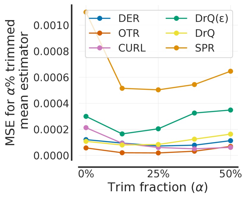
As an alternative to median, we recommend using the interquartile mean (IQM). Also called 25% trimmed mean, IQM discards the bottom and top of the runs and calculates the mean score of the remaining 50% runs (= for runs each on tasks). IQM interpolates between mean and median across runs, which are 0% and almost trimmed means respectively. Compared to sample median, IQM is a better indicator of overall performance as it is calculated using 50% of the combined runs while median only depends on the performance ordering across tasks and not on the magnitude except at most 2 tasks. For example, zero scores on nearly half of the tasks does not affect the median while IQM exhibits a severe degradation. Compared to mean, IQM is robust to outliers, yet has considerably less bias than median (Figure A.17). While median is more robust to outliers than IQM, this robustness comes at the expense of statistical efficiency, which is crucial in the few-run regime: IQM results in much smaller CIs (Figure 2 (right) and 6) and is able to detect a given improvement with far fewer runs (Figures 6 and A.16).
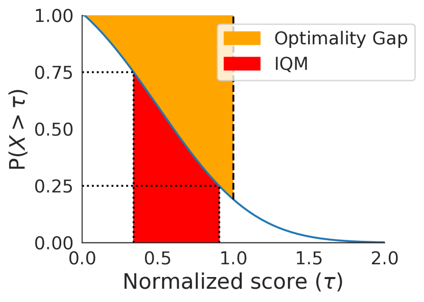
As a robust alternative to mean, we recommend using the optimality gap: the amount by which the algorithm fails to meet a minimum score of (orange region in Figure 8). This assumes that a score of 1.0 is a desirable target beyond which improvements are not very important, for example when the aim is to obtain human-level performance [e.g., 23, 3]. Naturally, the threshold may be chosen differently, which we discuss further in Appendix A.7.
If one is interested in knowing how robust an improvement from an algorithm over an algorithm is, another possible metric to consider is the average probability of improvement – this metric shows how likely it is for to outperform on a randomly selected task. Specifically, , where (Equation A.2) is the probability that is better than on task . Note that, unlike IQM and optimality gap, this metric does not account for the size of improvement. While finding the best aggregate metric is still an open question and is often dependent on underlying normalized score distribution, our proposed alternatives avoid the failure modes of prevalent metrics while being robust and requiring fewer runs to reduce uncertainty.
5 Re-evaluating Evaluation on Deep RL Benchmarks

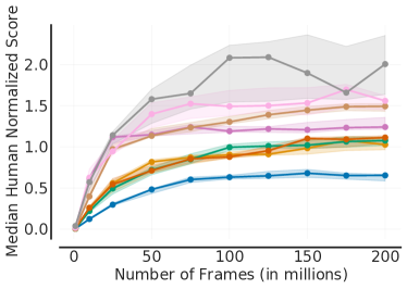
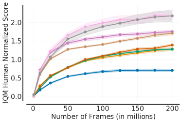
Arcade Learning Environment. Training RL agents for 200M frames on the ALE [5, 69] is the most widely recognized benchmark in deep RL. We revisit some popular methods which demonstrated progress on this benchmark and reveal discrepancies in their findings as a consequence of ignoring the uncertainty in their results (Figure 9). For example, DreamerV2 [38] exhibits a large amount of uncertainty in aggregate scores. While M-IQN [109] claimed better performance than Dopamine Rainbow888Dopamine Rainbow differs from that of Hessel et al. [42] by not including double DQN, dueling architecture and noisy networks. Also, results in [42] were reported using a single run without sticky actions. [42] in terms of median normalized scores, their interval estimates strikingly overlap. Similarly, while C51 [5] is considered substantially better than DQN [75], the interval estimates as well as performance profiles for DQN (Adam) and C51 overlap significantly.
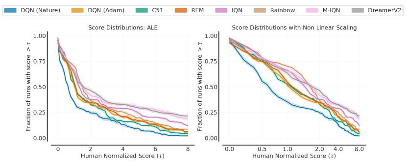
Figure 9 reveals an interesting limitation of aggregate metrics: depending on the choice of metric, the ordering between algorithms changes (e.g., Median vs. IQM). The inconsistency in ranking across aggregate metrics arises from the fact that such metrics only capture a specific aspect of overall performance across tasks and runs. Additionally, the change of algorithm ranking between optimality gap and IQM/median scores reveal that while recent algorithms typically show performance gains relative to humans on average, their performance seems to be worse on games below human performance. Since performance profiles capture the full picture, they would often illustrate why such inconsistencies exist. For example, optimality gap and IQM can be both read as areas in the profile (Figure 8). The performance profile in Figure 10 (left) illustrates the nuances present when comparing different algorithms. For example, IQN seems to be better than Rainbow for , but worse for . Similarly, the profiles of DreamerV2 and M-IQN for intersect at multiple points. To compare sample efficiency of the agents, we also present their IQM scores as a function of number of frames in Figure 10 (right).

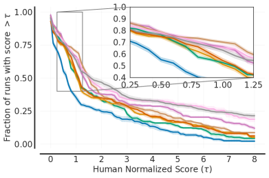

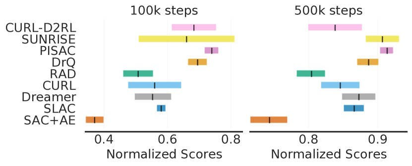
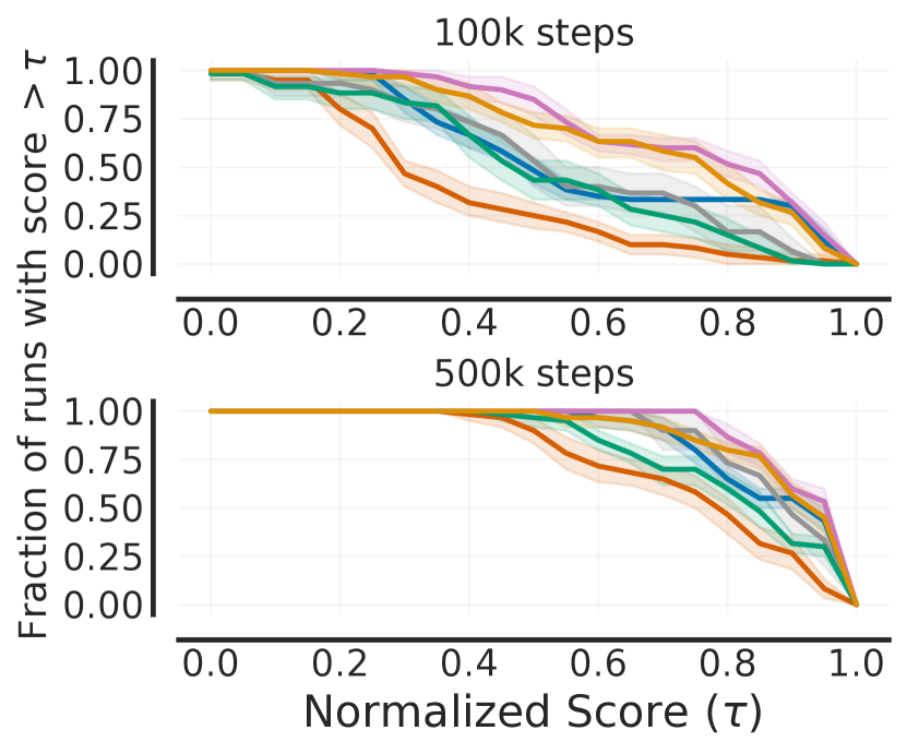
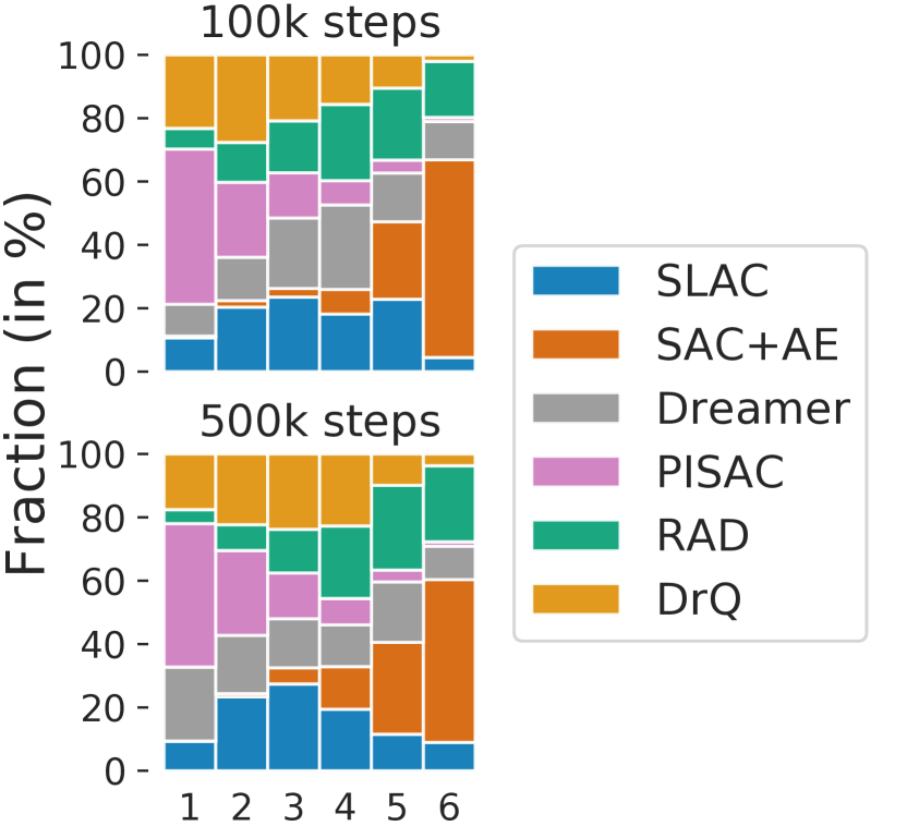
DeepMind Control Suite. Recent continuous control papers benchmark performance on 6 tasks in DM Control [104] at 100k and 500k steps. Typically, such papers claim improvement based on higher mean scores per task regardless of the variability in those scores. However, we find that when accounting for uncertainty in results, most algorithms do not consistently rank above algorithms they claimed to improve upon (Figure 11(c) and 11(b)). Furthermore, there are huge overlaps in 95% CIs of mean normalized scores for most algorithms (Figure 11(a)). These findings suggest that a lot of the reported improvements are spurious, resulting from randomness in the experimental protocol.
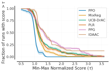
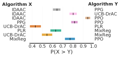
Procgen benchmark. Procgen [18] is a popular benchmark, consisting of 16 diverse tasks, for evaluating generalization in RL. Recent papers report mean PPO-normalized scores on this benchmark to emphasize the gains relative to PPO [92] as most methods are built on top of it. However, Figure 12 (left) shows that PPO-normalized scores typically have a heavy-tailed distribution making the mean scores highly dependent on performance on a small fraction of tasks. Instead, we recommend using normalization based on the estimated minimum and maximum scores on ProcGen [18] and reporting aggregate metrics based on such scores (Figure A.32). While publications sometimes make binary claims about whether they improve over prior methods, such improvements are inherently probabilistic. To reveal this discrepancy, we investigate the following question: “What is the probability that an algorithm which claimed improvement over a prior algorithm performs better than it?” (Figure 12, right). While this probability does not distinguish between two algorithms which uniformly improve on all tasks by 1% and 100%, it does highlight how likely an improvement is. For example, there is only a % chance that UCB-DrAC [81] improves upon PLR [48]. We note that a number of improvements reported in the existing literature are only % likely.
6 Discussion
We saw, both in our case study on the Atari 100k benchmark and with our analysis of other widely-used RL benchmarks, that statistical issues can have a sizeable influence on reported results, in particular when point estimates are used or evaluation protocols are not kept constant within comparisons. Despite earlier calls for more experimental rigor in deep RL [41, 20, 21, 49, 16, 83] (discussed in Appendix A.3), our analysis shows that the field has not yet found sure footing in this regards.
In part, this is because the issue of reproducibility is a complex one; where our work is concerned with our confidence about and interpretation of reported results (what Goodman et al. [34] calls results reproducibility), others [79] have highlighted that there might be missing information about the experiments themselves (methods reproducibility). We remark that the problem is not solved by fixing random seeds, as has sometimes been proposed [77, 52], since it does not really address the question of whether an algorithm would perform well under similar conditions but with different seeds. Furthermore, fixed seeds might benefit certain algorithms more than others. Nor can the problem be solved by the use of dichotomous statistical significance tests, as discussed in Section 2.
One way to minimize the risks associated with statistical effects is to report results in a more complete fashion, paying close attention to bias and uncertainty within these estimates. To this end, our recommendations are summarized in Table 1. To further support RL researchers in this endeavour, we released an easy-to-use Python library, rliable along with a Colab notebook for implementing our recommendations, as well as all the individual runs used in our experiments999Colab: bit.ly/statistical_precipice_colab. Individual runs: gs://rl-benchmark-data.. Again, we emphasize the importance of published papers providing results for all runs to allow for future statistical analyses.
A barrier to adoption of evaluation protocols proposed in this work, and more generally, rigorous evaluation, is whether there are clear incentives for researchers to do so, as more rigor generally entails more nuanced and tempered claims. Arguably, doing good and reproducible science is one such incentive. We hope that our findings about erroneous conclusions in published papers would encourage researchers to avoid fooling themselves, even if that requires tempered claims. That said, a more pragmatic incentive would be if conferences and reviewers required more rigorous evaluation for publication, e.g., NeurIPS 2021 checklist asks whether error bars are reported. Moving towards reliable evaluation is an ongoing process and we believe that this paper would greatly benefit it.
Given the substantial influence of statistical considerations in experiments involving 40-year old Atari 2600 video games and low-DOF robotic simulations, we argue that it is unlikely that an increase in available computation will resolve the problem for the future generation of RL benchmarks. Instead, just as a well-prepared rock-climber can skirt the edge of the steepest precipices, it seems likely that ongoing progress in reinforcement learning will require greater experimental discipline.
Societal Impacts
This paper calls for statistical sophistication in deep RL research by accounting for statistical uncertainty in reported results. However, statistical sophistication can introduce new forms of statistical abuses and monitoring the literature for such abuses should be an ongoing priority for the research community. Moving towards reliable evaluation and reproducible research is an ongoing process and this paper only partly addresses it by providing tools for more reliable evaluation. That said, while accounting for uncertainty in results is not a panacea, it provides a strong foundation for trustworthy results on which the community can build upon, with increased confidence. In terms of broader societal impact of this work, we do not see any foreseeable strongly negative impacts. However, this paper could positively impact society by constituting a step forwards in rigorous few-run evaluation regime, which reduces computational burden on researchers and is ‘‘greener’’ than evaluating a large number of runs.
Acknowledgments
We thank Xavier Bouthillier, Dumitru Erhan, Marlos C. Machado, David Ha, Fabio Viola, Fernando Diaz, Stephanie Chan, Jacob Buckman, Danijar Hafner and anonymous NeurIPS’ reviewers for providing valuable feedback for an earlier draft of this work. We also acknowledge Matteo Hessel, David Silver, Tom Schaul, Csaba Szepesvári, Hado van Hasselt, Rosanne Liu, Simon Kornblith, Aviral Kumar, George Tucker, Kevin Murphy, Ankit Anand, Aravind Srinivas, Matthew Botvinick, Clare Lyle, Kimin Lee, Misha Laskin, Ankesh Anand, Joelle Pineau and Braham Synder for helpful discussions. We also thank all the authors who provided individual runs for their corresponding publications. We are also grateful for general support from Google Research teams in Montréal and elsewhere.
References
- Agarwal et al. [2020] Rishabh Agarwal, Dale Schuurmans, and Mohammad Norouzi. An optimistic perspective on offline reinforcement learning. In International Conference on Machine Learning, 2020.
- Amrhein et al. [2019] Valentin Amrhein, Sander Greenland, and Blake McShane. Scientists rise up against statistical significance. Nature, 2019.
- Badia et al. [2020] Adrià Puigdomènech Badia, Bilal Piot, Steven Kapturowski, Pablo Sprechmann, Alex Vitvitskyi, Zhaohan Daniel Guo, and Charles Blundell. Agent57: Outperforming the atari human benchmark. In International Conference on Machine Learning, pages 507--517. PMLR, 2020.
- Baker [2016] Monya Baker. 1,500 scientists lift the lid on reproducibility. Nature News, 2016.
- Bellemare et al. [2013] Marc G Bellemare, Yavar Naddaf, Joel Veness, and Michael Bowling. The arcade learning environment: An evaluation platform for general agents. Journal of Artificial Intelligence Research, 47:253--279, 2013.
- Bellemare et al. [2017] Marc G Bellemare, Will Dabney, and Rémi Munos. A distributional perspective on reinforcement learning. In International Conference on Machine Learning, pages 449--458. PMLR, 2017.
- Bellemare et al. [2020] Marc G Bellemare, Salvatore Candido, Pablo Samuel Castro, Jun Gong, Marlos C Machado, Subhodeep Moitra, Sameera S Ponda, and Ziyu Wang. Autonomous navigation of stratospheric balloons using reinforcement learning. Nature, 2020.
- Berner et al. [2019] Christopher Berner, Greg Brockman, Brooke Chan, Vicki Cheung, Przemysław Dębiak, Christy Dennison, David Farhi, Quirin Fischer, Shariq Hashme, Chris Hesse, et al. Dota 2 with large scale deep reinforcement learning. arXiv preprint arXiv:1912.06680, 2019.
- Bickel et al. [2012] Peter J Bickel, Friedrich Götze, and Willem R van Zwet. Resampling fewer than n observations: gains, losses, and remedies for losses. In Selected works of Willem van Zwet, pages 267--297. Springer, 2012.
- Birattari and Dorigo [2007] Mauro Birattari and Marco Dorigo. How to assess and report the performance of a stochastic algorithm on a benchmark problem: mean or best result on a number of runs? Optimization letters, 2007.
- Bouthillier et al. [2019] Xavier Bouthillier, César Laurent, and Pascal Vincent. Unreproducible research is reproducible. In International Conference on Machine Learning, pages 725--734, 2019.
- Bouthillier et al. [2021] Xavier Bouthillier, Pierre Delaunay, Mirko Bronzi, Assya Trofimov, Brennan Nichyporuk, Justin Szeto, Nazanin Mohammadi Sepahvand, Edward Raff, Kanika Madan, Vikram Voleti, et al. Accounting for variance in machine learning benchmarks. Proceedings of Machine Learning and Systems, 3, 2021.
- Bradbury et al. [2018] James Bradbury, Roy Frostig, Peter Hawkins, Matthew James Johnson, Chris Leary, Dougal Maclaurin, George Necula, Adam Paszke, Jake VanderPlas, Skye Wanderman-Milne, and Qiao Zhang. JAX: composable transformations of Python+NumPy programs, 2018. URL http://github.com/google/jax.
- Castro et al. [2018] Pablo Samuel Castro, Subhodeep Moitra, Carles Gelada, Saurabh Kumar, and Marc G Bellemare. Dopamine: A research framework for deep reinforcement learning. arXiv preprint arXiv:1812.06110, 2018.
- Ceron and Castro [2021] Johan Samir Obando Ceron and Pablo Samuel Castro. Revisiting rainbow: Promoting more insightful and inclusive deep reinforcement learning research. In International Conference on Machine Learning, 2021.
- Chan et al. [2020] Stephanie CY Chan, Samuel Fishman, Anoop Korattikara, John Canny, and Sergio Guadarrama. Measuring the reliability of reinforcement learning algorithms. In International Conference on Learning Representations, 2020.
- Clary et al. [2019] Kaleigh Clary, Emma Tosch, John Foley, and David Jensen. Let’s play again: Variability of deep reinforcement learning agents in atari environments. arXiv preprint arXiv:1904.06312, 2019.
- Cobbe et al. [2020a] Karl Cobbe, Chris Hesse, Jacob Hilton, and John Schulman. Leveraging procedural generation to benchmark reinforcement learning. In International conference on machine learning, pages 2048--2056. PMLR, 2020a.
- Cobbe et al. [2020b] Karl Cobbe, Jacob Hilton, Oleg Klimov, and John Schulman. Phasic policy gradient. arXiv preprint arXiv:2009.04416, 2020b.
- Colas et al. [2018] Cédric Colas, Olivier Sigaud, and Pierre-Yves Oudeyer. How many random seeds? statistical power analysis in deep reinforcement learning experiments. arXiv preprint arXiv:1806.08295, 2018.
- Colas et al. [2019] Cédric Colas, Olivier Sigaud, and Pierre-Yves Oudeyer. A hitchhiker’s guide to statistical comparisons of reinforcement learning algorithms. arXiv preprint arXiv:1904.06979, 2019.
- Dabney et al. [2018a] Will Dabney, Georg Ostrovski, David Silver, and Rémi Munos. Implicit quantile networks for distributional reinforcement learning. In International conference on machine learning, pages 1096--1105. PMLR, 2018a.
- Dabney et al. [2018b] Will Dabney, Mark Rowland, Marc G Bellemare, and Rémi Munos. Distributional reinforcement learning with quantile regression. In Thirty-Second AAAI Conference on Artificial Intelligence, 2018b.
- Dehghani et al. [2021] Mostafa Dehghani, Yi Tay, Alexey A Gritsenko, Zhe Zhao, Neil Houlsby, Fernando Diaz, Donald Metzler, and Oriol Vinyals. The benchmark lottery. arXiv preprint arXiv:2107.07002, 2021.
- Dodge et al. [2020] Jesse Dodge, Gabriel Ilharco, Roy Schwartz, Ali Farhadi, Hannaneh Hajishirzi, and Noah Smith. Fine-tuning pretrained language models: Weight initializations, data orders, and early stopping. arXiv preprint arXiv:2002.06305, 2020.
- Dolan and Moré [2002] Elizabeth D Dolan and Jorge J Moré. Benchmarking optimization software with performance profiles. Mathematical programming, 91(2):201--213, 2002.
- Dror et al. [2019] Rotem Dror, Segev Shlomov, and Roi Reichart. Deep dominance-how to properly compare deep neural models. In Proceedings of the 57th Annual Meeting of the Association for Computational Linguistics, 2019.
- Ecoffet et al. [2019] Adrien Ecoffet, Joost Huizinga, Joel Lehman, Kenneth O Stanley, and Jeff Clune. Go-explore: a new approach for hard-exploration problems. arXiv preprint arXiv:1901.10995, 2019.
- Efron [1979] Bradley Efron. Bootstrap methods: another look at the jackknife. The Annals of Statistics, 7:1--26, 1979.
- Efron [1987] Bradley Efron. Better bootstrap confidence intervals. Journal of the American statistical Association, 1987.
- Ernst et al. [2005] Damien Ernst, Pierre Geurts, and Louis Wehenkel. Tree-based batch mode reinforcement learning. Journal of Machine Learning Research, 6:503--556, 2005.
- Espeholt et al. [2018] Lasse Espeholt, Hubert Soyer, Remi Munos, Karen Simonyan, Vlad Mnih, Tom Ward, Yotam Doron, Vlad Firoiu, Tim Harley, Iain Dunning, et al. Impala: Scalable distributed deep-rl with importance weighted actor-learner architectures. In International Conference on Machine Learning. PMLR, 2018.
- Gigerenzer [2018] Gerd Gigerenzer. Statistical rituals: The replication delusion and how we got there. Advances in Methods and Practices in Psychological Science, 1(2):198--218, 2018.
- Goodman et al. [2016] Steven N Goodman, Daniele Fanelli, and John PA Ioannidis. What does research reproducibility mean? Science translational medicine, 8(341):341ps12--341ps12, 2016.
- Greenland et al. [2016] Sander Greenland, Stephen J Senn, Kenneth J Rothman, John B Carlin, Charles Poole, Steven N Goodman, and Douglas G Altman. Statistical tests, p values, confidence intervals, and power: a guide to misinterpretations. European journal of epidemiology, 2016.
- Haarnoja et al. [2018] Tuomas Haarnoja, Aurick Zhou, Pieter Abbeel, and Sergey Levine. Soft actor-critic: Off-policy maximum entropy deep reinforcement learning with a stochastic actor. In International Conference on Machine Learning, pages 1861--1870. PMLR, 2018.
- Hafner et al. [2019] Danijar Hafner, Timothy Lillicrap, Jimmy Ba, and Mohammad Norouzi. Dream to control: Learning behaviors by latent imagination. In International Conference on Learning Representations, 2019.
- Hafner et al. [2020] Danijar Hafner, Timothy Lillicrap, Mohammad Norouzi, and Jimmy Ba. Mastering atari with discrete world models. arXiv preprint arXiv:2010.02193, 2020.
- Hansen et al. [2020] Steven Hansen, Will Dabney, Andre Barreto, David Warde-Farley, Tom Van de Wiele, and Volodymyr Mnih. Fast task inference with variational intrinsic successor features. In International Conference on Learning Representations, 2020.
- Helwig [2021] Nathaniel E Helwig. Bootstrap Confidence Intervals, 01 2021. URL http://users.stat.umn.edu/~helwig/notes/npboot-notes.html#bootstrap-confidence-intervals.
- Henderson et al. [2018] Peter Henderson, Riashat Islam, Philip Bachman, Joelle Pineau, Doina Precup, and David Meger. Deep reinforcement learning that matters. In Proceedings of the AAAI Conference on Artificial Intelligence, 2018.
- Hessel et al. [2018] Matteo Hessel, Joseph Modayil, Hado Van Hasselt, Tom Schaul, Georg Ostrovski, Will Dabney, Dan Horgan, Bilal Piot, Mohammad Azar, and David Silver. Rainbow: Combining improvements in deep reinforcement learning. In Proceedings of the AAAI Conference on Artificial Intelligence, 2018.
- Hessel et al. [2021] Matteo Hessel, Ivo Danihelka, Fabio Viola, Arthur Guez, Simon Schmitt, Laurent Sifre, Theophane Weber, David Silver, and Hado van Hasselt. Muesli: Combining improvements in policy optimization. Proceedings of the 38th International Conference on Machine Learning, 2021.
- Ioannidis [2005] John PA Ioannidis. Why most published research findings are false. PLoS medicine, 2(8):e124, 2005.
- Irpan [2018] Alex Irpan. Deep reinforcement learning doesn’t work yet. https://www.alexirpan.com/2018/02/14/rl-hard.html, 2018.
- Islam et al. [2017] Riashat Islam, Peter Henderson, Maziar Gomrokchi, and Doina Precup. Reproducibility of benchmarked deep reinforcement learning tasks for continuous control. arXiv preprint arXiv:1708.04133, 2017.
- Jaderberg et al. [2016] Max Jaderberg, Volodymyr Mnih, Wojciech Marian Czarnecki, Tom Schaul, Joel Z Leibo, David Silver, and Koray Kavukcuoglu. Reinforcement learning with unsupervised auxiliary tasks. arXiv preprint arXiv:1611.05397, 2016.
- Jiang et al. [2021] Minqi Jiang, Ed Grefenstette, and Tim Rocktäschel. Prioritized level replay. International Conference on Machine Learning, 2021.
- Jordan et al. [2020] Scott Jordan, Yash Chandak, Daniel Cohen, Mengxue Zhang, and Philip Thomas. Evaluating the performance of reinforcement learning algorithms. In International Conference on Machine Learning, pages 4962--4973. PMLR, 2020.
- Kaiser et al. [2019] Lukasz Kaiser, Mohammad Babaeizadeh, Piotr Milos, Blazej Osinski, Roy H Campbell, Konrad Czechowski, Dumitru Erhan, Chelsea Finn, Piotr Kozakowski, Sergey Levine, et al. Model-based reinforcement learning for atari. arXiv preprint arXiv:1903.00374, 2019.
- Kielak [2020] Kacper Kielak. Do recent advancements in model-based deep reinforcement learning really improve data efficiency? arXiv preprint arXiv:2003.10181, 2020.
- Kolesnikov and Hrinchuk [2019] Sergey Kolesnikov and Oleksii Hrinchuk. Catalyst. rl: a distributed framework for reproducible rl research. arXiv preprint arXiv:1903.00027, 2019.
- Kostrikov* et al. [2021] Ilya Kostrikov*, Denis Yarats*, and Rob Fergus. Image augmentation is all you need: Regularizing deep reinforcement learning from pixels. In International Conference on Learning Representations, 2021.
- Kozakowski et al. [2021] Piotr Kozakowski, Lukasz Kaiser, Henryk Michalewski, Afroz Mohiuddin, and Katarzyna Kańska. Q-value weighted regression: Reinforcement learning with limited data. arXiv preprint arXiv:2102.06782, 2021.
- Kulkarni et al. [2019] Tejas D Kulkarni, Ankush Gupta, Catalin Ionescu, Sebastian Borgeaud, Malcolm Reynolds, Andrew Zisserman, and Volodymyr Mnih. Unsupervised learning of object keypoints for perception and control. NeurIPS, 32:10724--10734, 2019.
- Laskin et al. [2020a] Michael Laskin, Aravind Srinivas, and Pieter Abbeel. Curl: Contrastive unsupervised representations for reinforcement learning. In International Conference on Machine Learning, 2020a.
- Laskin et al. [2020b] Misha Laskin, Kimin Lee, Adam Stooke, Lerrel Pinto, Pieter Abbeel, and Aravind Srinivas. Reinforcement learning with augmented data. Advances in Neural Information Processing Systems, 2020b.
- Lee et al. [2020a] Alex Lee, Anusha Nagabandi, Pieter Abbeel, and Sergey Levine. Stochastic latent actor-critic: Deep reinforcement learning with a latent variable model. Advances in Neural Information Processing Systems, 33, 2020a.
- Lee et al. [2021] Kimin Lee, Michael Laskin, Aravind Srinivas, and Pieter Abbeel. Sunrise: A simple unified framework for ensemble learning in deep reinforcement learning. International Conference on Machine Learning, 2021.
- Lee et al. [2020b] Kuang-Huei Lee, Ian Fischer, Anthony Liu, Yijie Guo, Honglak Lee, John Canny, and Sergio Guadarrama. Predictive information accelerates learning in rl. Advances in Neural Information Processing Systems, 2020b.
- Levy [1992] Haim Levy. Stochastic dominance and expected utility: Survey and analysis. Management science, 38(4):555--593, 1992.
- Lillicrap et al. [2015] Timothy P Lillicrap, Jonathan J Hunt, Alexander Pritzel, Nicolas Heess, Tom Erez, Yuval Tassa, David Silver, and Daan Wierstra. Continuous control with deep reinforcement learning. arXiv preprint arXiv:1509.02971, 2015.
- Lin et al. [2021] Jimmy Lin, Daniel Campos, Nick Craswell, Bhaskar Mitra, and Emine Yilmaz. Significant improvements over the state of the art? a case study of the ms marco document ranking leaderboard. arXiv preprint arXiv:2102.12887, 2021.
- Liu et al. [2021] Guoqing Liu, Chuheng Zhang, Li Zhao, Tao Qin, Jinhua Zhu, Li Jian, Nenghai Yu, and Tie-Yan Liu. Return-based contrastive representation learning for reinforcement learning. In International Conference on Learning Representations, 2021.
- Liu and Abbeel [2021a] Hao Liu and Pieter Abbeel. Behavior from the void: Unsupervised active pre-training. arXiv preprint arXiv:2103.04551, 2021a.
- Liu and Abbeel [2021b] Hao Liu and Pieter Abbeel. Aps: Active pretraining with successor features. In Proceedings of the 38th International Conference on Machine Learning, 2021b.
- Lucic et al. [2017] Mario Lucic, Karol Kurach, Marcin Michalski, Sylvain Gelly, and Olivier Bousquet. Are gans created equal? a large-scale study. arXiv preprint arXiv:1711.10337, 2017.
- Lynnerup et al. [2020] Nicolai A Lynnerup, Laura Nolling, Rasmus Hasle, and John Hallam. A survey on reproducibility by evaluating deep reinforcement learning algorithms on real-world robots. In Conference on Robot Learning, 2020.
- Machado et al. [2018] Marlos C Machado, Marc G Bellemare, Erik Talvitie, Joel Veness, Matthew Hausknecht, and Michael Bowling. Revisiting the arcade learning environment: Evaluation protocols and open problems for general agents. Journal of Artificial Intelligence Research, 2018.
- Mania et al. [2018] Horia Mania, Aurelia Guy, and Benjamin Recht. Simple random search provides a competitive approach to reinforcement learning. arXiv preprint arXiv:1803.07055, 2018.
- Mann and Whitney [1947] Henry B Mann and Donald R Whitney. On a test of whether one of two random variables is stochastically larger than the other. The annals of mathematical statistics, pages 50--60, 1947.
- Maulana and Lee [2021] Muhammad Rizki Maulana and Wee Sun Lee. Ensemble and auxiliary tasks for data-efficient deep reinforcement learning. arXiv preprint arXiv:2107.01904, 2021.
- McShane et al. [2019] Blakeley B McShane, David Gal, Andrew Gelman, Christian Robert, and Jennifer L Tackett. Abandon statistical significance. The American Statistician, 2019.
- Melis et al. [2018] Gábor Melis, Chris Dyer, and Phil Blunsom. On the state of the art of evaluation in neural language models. In International Conference on Learning Representations, 2018.
- Mnih et al. [2015] Volodymyr Mnih, Koray Kavukcuoglu, David Silver, Andrei A Rusu, Joel Veness, Marc G Bellemare, Alex Graves, Martin Riedmiller, Andreas K Fidjeland, Georg Ostrovski, et al. Human-level control through deep reinforcement learning. Nature, 2015.
- Mnih et al. [2016] Volodymyr Mnih, Adria Puigdomenech Badia, Mehdi Mirza, Alex Graves, Timothy Lillicrap, Tim Harley, David Silver, and Koray Kavukcuoglu. Asynchronous methods for deep reinforcement learning. In International conference on machine learning, pages 1928--1937. PMLR, 2016.
- Nagarajan et al. [2018] Prabhat Nagarajan, Garrett Warnell, and Peter Stone. Deterministic implementations for reproducibility in deep reinforcement learning. arXiv preprint arXiv:1809.05676, 2018.
- Pashler and Wagenmakers [2012] Harold Pashler and Eric-Jan Wagenmakers. Editors’ introduction to the special section on replicability in psychological science: A crisis of confidence? Perspectives on psychological science, 7(6):528--530, 2012.
- Pineau et al. [2020] Joelle Pineau, Philippe Vincent-Lamarre, Koustuv Sinha, Vincent Larivière, Alina Beygelzimer, Florence d’Alché Buc, Emily Fox, and Hugo Larochelle. Improving reproducibility in machine learning research (a report from the neurips 2019 reproducibility program). arXiv preprint arXiv:2003.12206, 2020.
- Raileanu and Fergus [2021] Roberta Raileanu and Rob Fergus. Decoupling value and policy for generalization in reinforcement learning. International Conference on Machine Learning, 2021.
- Raileanu et al. [2020] Roberta Raileanu, Max Goldstein, Denis Yarats, Ilya Kostrikov, and Rob Fergus. Automatic data augmentation for generalization in deep reinforcement learning. arXiv preprint arXiv:2006.12862, 2020.
- Raposo et al. [2021] David Raposo, Sam Ritter, Adam Santoro, Greg Wayne, Theophane Weber, Matt Botvinick, Hado van Hasselt, and Francis Song. Synthetic returns for long-term credit assignment. arXiv preprint arXiv:2102.12425, 2021.
- Recht [2018] Ben Recht. Benchmarking Machine Learning with Performance Profiles, 03 2018. URL http://www.argmin.net/2018/03/26/performance-profiles/.
- Reimers and Gurevych [2017] Nils Reimers and Iryna Gurevych. Reporting score distributions makes a difference: Performance study of lstm-networks for sequence tagging. In Proceedings of the 2017 Conference on Empirical Methods in Natural Language Processing, pages 338--348, 2017.
- Ritter et al. [2017] Samuel Ritter, David GT Barrett, Adam Santoro, and Matt M Botvinick. Cognitive psychology for deep neural networks: A shape bias case study. In International conference on machine learning, 2017.
- Robine et al. [2020] Jan Robine, Tobias Uelwer, and Stefan Harmeling. Smaller world models for reinforcement learning. arXiv preprint arXiv:2010.05767, 2020.
- Romer [2020] David Romer. In praise of confidence intervals. In AEA Papers and Proceedings, volume 110, pages 55--60, 2020.
- Salimans et al. [2017] Tim Salimans, Jonathan Ho, Xi Chen, Szymon Sidor, and Ilya Sutskever. Evolution strategies as a scalable alternative to reinforcement learning. arXiv preprint arXiv:1703.03864, 2017.
- Saphal et al. [2021] Rohan Saphal, Balaraman Ravindran, Dheevatsa Mudigere, Sasikant Avancha, and Bharat Kaul. Seerl: Sample efficient ensemble reinforcement learning. In Proceedings of the 20th International Conference on Autonomous Agents and MultiAgent Systems, pages 1100--1108, 2021.
- Schaul et al. [2021] Tom Schaul, Georg Ostrovski, Iurii Kemaev, and Diana Borsa. Return-based scaling: Yet another normalisation trick for deep rl. arXiv preprint arXiv:2105.05347, 2021.
- Schrittwieser et al. [2020] Julian Schrittwieser, Ioannis Antonoglou, Thomas Hubert, Karen Simonyan, Laurent Sifre, Simon Schmitt, Arthur Guez, Edward Lockhart, Demis Hassabis, Thore Graepel, et al. Mastering atari, go, chess and shogi by planning with a learned model. Nature, 2020.
- Schulman et al. [2017] John Schulman, Filip Wolski, Prafulla Dhariwal, Alec Radford, and Oleg Klimov. Proximal policy optimization algorithms. arXiv preprint arXiv:1707.06347, 2017.
- Schwarzer et al. [2021] Max Schwarzer, Ankesh Anand, Rishab Goel, R Devon Hjelm, Aaron Courville, and Philip Bachman. Data-efficient reinforcement learning with self-predictive representations. In International Conference on Learning Representations, 2021.
- Sellam et al. [2021] Thibault Sellam, Steve Yadlowsky, Jason Wei, Naomi Saphra, Alexander D’Amour, Tal Linzen, Jasmijn Bastings, Iulia Turc, Jacob Eisenstein, Dipanjan Das, et al. The multiberts: Bert reproductions for robustness analysis. arXiv preprint arXiv:2106.16163, 2021.
- Seo et al. [2021] Younggyo Seo, Lili Chen, Jinwoo Shin, Honglak Lee, Pieter Abbeel, and Kimin Lee. State entropy maximization with random encoders for efficient exploration. In Proceedings of the 38th International Conference on Machine Learning, 2021.
- Silver et al. [2016] David Silver, Aja Huang, Chris J Maddison, Arthur Guez, Laurent Sifre, George Van Den Driessche, Julian Schrittwieser, Ioannis Antonoglou, Veda Panneershelvam, Marc Lanctot, et al. Mastering the game of go with deep neural networks and tree search. nature, 529(7587):484--489, 2016.
- Sinha et al. [2020] Samarth Sinha, Homanga Bharadhwaj, Aravind Srinivas, and Animesh Garg. D2rl: Deep dense architectures in reinforcement learning. arXiv preprint arXiv:2010.09163, 2020.
- Srinivas et al. [2020] Aravind Srinivas, Michael Laskin, and Pieter Abbeel. Curl: Contrastive unsupervised representations for reinforcement learning. arXiv preprint arXiv:2004.04136v2, 2020.
- Sutton [1988] Richard S Sutton. Learning to predict by the methods of temporal differences. Machine learning, 3(1):9--44, 1988.
- Sutton [1996] Richard S Sutton. Generalization in reinforcement learning: Successful examples using sparse coarse coding. Advances in neural information processing systems, 1996.
- Sutton and Barto [2018] Richard S. Sutton and Andrew G. Barto. Reinforcement learning: An introduction. MIT Press, 2nd edition, 2018.
- Sutton et al. [1999] Richard S Sutton, Doina Precup, and Satinder Singh. Between mdps and semi-mdps: A framework for temporal abstraction in reinforcement learning. Artificial intelligence, 1999.
- Szita and Lörincz [2006] István Szita and András Lörincz. Learning tetris using the noisy cross-entropy method. Neural computation, 2006.
- Tassa et al. [2018] Yuval Tassa, Yotam Doron, Alistair Muldal, Tom Erez, Yazhe Li, Diego de Las Casas, David Budden, Abbas Abdolmaleki, Josh Merel, Andrew Lefrancq, et al. Deepmind control suite. arXiv preprint arXiv:1801.00690, 2018.
- Toromanoff et al. [2019] Marin Toromanoff, Emilie Wirbel, and Fabien Moutarde. Is deep reinforcement learning really superhuman on atari? leveling the playing field. arXiv preprint arXiv:1908.04683, 2019.
- Tukey [1960] John W Tukey. A survey of sampling from contaminated distributions. Contributions to probability and statistics, pages 448--485, 1960.
- van Hasselt et al. [2019] Hado van Hasselt, Matteo Hessel, and John Aslanides. When to use parametric models in reinforcement learning? NeurIPS, 2019.
- Varoquaux and Cheplygina [2021] Gaël Varoquaux and Veronika Cheplygina. How i failed machine learning in medical imaging--shortcomings and recommendations. arXiv preprint arXiv:2103.10292, 2021.
- Vieillard et al. [2020] Nino Vieillard, Olivier Pietquin, and Matthieu Geist. Munchausen reinforcement learning. Advances in Neural Information Processing Systems, 33, 2020.
- Vinyals et al. [2019] Oriol Vinyals, Igor Babuschkin, Wojciech M Czarnecki, Michaël Mathieu, Andrew Dudzik, Junyoung Chung, David H Choi, Richard Powell, Timo Ewalds, Petko Georgiev, et al. Grandmaster level in starcraft ii using multi-agent reinforcement learning. Nature, 2019.
- Wang et al. [2020] Kaixin Wang, Bingyi Kang, Jie Shao, and Jiashi Feng. Improving generalization in reinforcement learning with mixture regularization. arXiv preprint arXiv:2010.10814, 2020.
- Wasserstein et al. [2019] Ronald L. Wasserstein, Allen L. Schirm, and Nicole A. Lazar. Moving to a world beyond “p < 0.05”. The American Statistician, 2019.
- Welch [1947] Bernard L Welch. The generalization ofstudent’s’ problem when several different population variances are involved. Biometrika, 34(1/2):28--35, 1947.
- Yarats et al. [2019] Denis Yarats, Amy Zhang, Ilya Kostrikov, Brandon Amos, Joelle Pineau, and Rob Fergus. Improving sample efficiency in model-free reinforcement learning from images. arXiv preprint arXiv:1910.01741, 2019.
- Zhu et al. [2020] Jinhua Zhu, Yingce Xia, Lijun Wu, Jiajun Deng, Wengang Zhou, Tao Qin, and Houqiang Li. Masked contrastive representation learning for reinforcement learning. arXiv preprint arXiv:2010.07470, 2020.
- Zhuang et al. [2021] Donglin Zhuang, Xingyao Zhang, Shuaiwen Leon Song, and Sara Hooker. Randomness in neural network training: Characterizing the impact of tooling. arXiv preprint arXiv:2106.11872, 2021.
Appendix A Appendix
A.1 Open-source notebook and data
Colab notebook for producing and analyzing performance profiles, robust aggregate metrics, and interval estimates based on stratified bootstrap CIs, as well as replicating the results in the paper can be found at bit.ly/statistical_precipice_colab.
Individual runs for Atari 100k. We released the 100 runs per game for each of the 6 algorithms in the case study in a public cloud bucket at gs://rl-benchmark-data/atari_100k.
Individual runs for ALE, Procgen and DM Control. For ALE, we used the individual runs from Dopamine [14] baselines except for DreamerV2 [38], REM [1] and M-IQN [109], for which the individual run scores were obtained from the corresponding authors. We release all the individual run scores as well as final scores for ALE at gs://rl-benchmark-data/ALE. The Procgen results were obtained from the authors of IDAAC [80] and MixReg [48] and are released at gs://rl-benchmark-data/procgen. For DM Control101010Dreamer [37] results on DM control, obtained from the corresponding author, are based on hyperparameters tuned for sample-efficiency. Compared to the original paper [37], the actor-critic learning rates were increased to , the amount of free bits to 1.5, the training frequency, and the amount of pre-training to 1k steps on 10k randomly collected frames. The imagination horizon was decreased to 10., all the runs were obtained from the corresponding authors and are released at gs://rl-benchmark-data/dm_control.
See agarwl.github.io/rliable for a website for the paper.
A.2 Atari 100k: Additional Details and Results
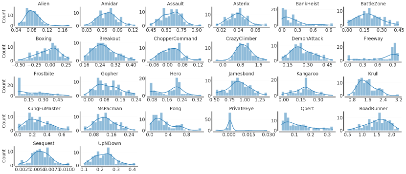
.
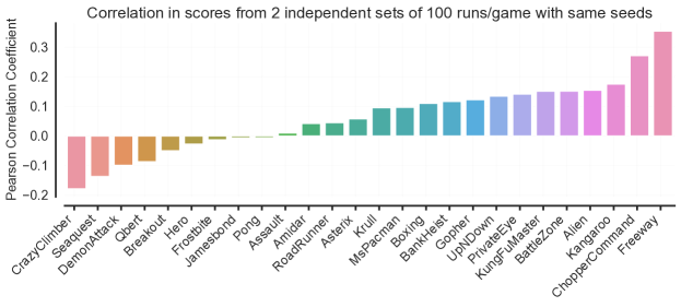
Code. Due to unavailability of open-source code for der, and otr for Atari 100k, we re-implemented these algorithms using Dopamine [14], a reproducible deep RL framework. For curl and spr, we used the open-source code released by the authors while for drq, we used the source-code obtained from the authors. Our code for Atari 100k experiments is open-sourced as part of the Dopamine library under the labs/atari_100k folder. We also released a JAX [13] implementation of the full Rainbow [42] in Dopamine.
Hyperparameters. All algorithms build upon the Rainbow [42] architecture and we use the exact same hyperparameters specified in the corresponding publication unless specified otherwise. Akin to drq and spr, we used -step returns with instead of for der. drq codebase uses non-standard evaluation hyperparameters, such as a 5% probability of selecting random actions during evaluation (-eval). drq differs drq in terms of using standard -greedy parameters [14, Table 1] including training decayed to 0.01 rather than 0.1 and evaluation set to 0.001 instead of 0.05. Refer to the gin configurations in labs/atari_100k/configs for more details.
Compute. For the case study on Atari 100k, we used Tesla P100 GPUs for all the runs. Each run spanned about 3-5 hours depending on the algorithm, and we ran a total of 100 runs / game 26 games/algorithm 6 algorithms = 15,600 runs. Additionally, we ran an additional 100 runs per game for der to compute a good approximation of point estimates for aggregate scores, which increases the total number of runs by 2600. Overall, we trained and evaluated 18,200 runs, which roughly amounts to 2400 days -- 3600 days of GPU training.
Comparing performance of two algorithms. When confidence intervals (CIs) overlap for two random variables and overlap, we estimate the CIs for to account for uncertainty in their difference (Figure A.16). For example, when using 5 runs, the median score improvement from drq over der is estimated to lie within while that of SPR over DrQ lies within . Furthermore, while improvement from SPR over DER with to runs is not statistically significant, claiming ‘‘no improvement’’ would be misleading as evaluating more runs indeed shows that the improvement is significant.
Analyzing efficiency and bias of IQM. Theoretically, trimmed means, are known to have higher statistical efficiency for mixed distributions and heavy-tailed distributions (Cauchy distribution), at the cost of lower efficiency for some other less heavily-tailed distributions (normal distribution) than mean, as shown by the seminal work of Tukey [106]. Empirically, on Atari 100k, IQM provides good statistically efficiency among trimmed estimators across different algorithms (Figure A.16) as well as has considerably small bias than median (c.f. Figure A.17 vs. Figure 3).

A.3 Related work on rigorous evaluation in deep RL
While prior work [46, 41, 68] highlights various reproducibility issues in policy-gradient methods, this paper focuses specifically on the reliability of evaluation procedures on RL benchmarks and provides an extensive analysis on common deep RL algorithms on widely-used benchmarks.
For more rigorous performance comparisons on a single RL task, Henderson et al. [41], Colas et al. [21] provide guidelines for statistical significance testing while Colas et al. [20] focuses on determining the minimum number of runs needed for such comparisons to be statistically significant. Instead, this paper focuses on reliable comparisons on a suite of tasks and mainly recommends reporting stratified bootstrap CIs due to the dichotomous nature and wide misinterpretation of statistical significance tests (see Remark in Section 2). Henderson et al. [41], Colas et al. [20, 21] also discuss bootstrap CIs but for reporting single task mean scores – however, 3-5 runs is a small sample size for bootstrapping: on Atari 100k, for achieving true coverage close to 95%, such CIs require at least 20-30 runs per task (Figure A.18) as opposed to 5-10 runs for stratified bootstrap CIs for aggregate metrics like median, mean and IQM (Figure A.19).
Chan et al. [16] propose metrics to measure the reliability of RL algorithms in terms of their stability during training and their variability and risk in returns across multiple episodes. While this paper focuses on reliability of evaluation itself, performance profiles showing the tail distribution of episodic returns, applicable for even a single task with multiple runs, can be useful for measuring reliability of an algorithm’s performance.
Jordan et al. [49] propose a game-theoretic evaluation procedure for ‘‘complete’’ algorithms that do not require any hyperparameter tuning and recommend evaluating between 1,000 to 10,000 runs per task to detect statistically significant results. Instead, this work focuses on reliably evaluating performance obtained after the hyperparameter tuning phase, even with just a handful of runs. That said, run-score distributions based on runs with different hyperparameter configurations might reveal sensitivity to hyperparameter tuning.
An alternative to score distributions, proposed by Recht [83], is to replace scores in a performance profile [26] by the probability that average task scores of a given method outperforms the best method (among a given set of methods), computed using the Welsh’s t-test [113]. However, this profile is (1) also a biased estimate, (2) less robust to outlier runs, (3) is insensitive to the size of performance differences, i.e., two methods that are uniformly 1% and 100% worse than the best method are assigned the same probability, (4) is only sensible when task score distributions are Gaussian, as required by Welsh’s t-test, and finally, (5) the ranking of methods depends on the specific set of methods being compared in such profiles.
A.4 Non-standard Evaluation Protocols Involving Maximum
Even when adequate number of runs are used, the use of non-standard evaluation protocols can result in misleading comparisons. Such protocols commonly involve the insertion of a maximum operation inside evaluation, across or within runs, leading to a positive bias in reported scores compared to the standard approach without the maximum.
One seemingly reasonable but faulty argument [10] for maximum across runs is that in a real-world application, one might wish to run an stochastic algorithm for runs and then select the best result. However, in this case, we are not discussing but another algorithm , which evaluates random runs of . If we are interested in , taking maximum over runs only considers a single run of . Since is itself stochastic, proper experimental methodology requires multiple runs of . Furthermore, because learning curves are not in general monotonic, results produced under the maximum-during-training protocol are in general incomparable with end-performance reported results. In addition, such protocols introduces an additional source of positive statistical bias, since the maximum of a set of random variables is a biased estimate of their true maximum.
On Atari 100k, curl [56] and sunrise [59] used non-standard evaluation protocols. curl reported the maximum performance over 10 different evaluations during training. As a result, natural variability in both evaluation itself and in the agent’s performance during training contribute to overestimation. Applying the same procedure to curl’s baseline DER leads to scores far above those reported for curl (Figure 6, ‘‘der (curl’s protocol)’’). In the case of sunrise, the maximum was taken over eight hyperparameter configurations separately for each game, with three runs each. We simulate this procedure for der (also sunrise’s baseline), using a dummy hyperparameter. We find that a lot of sunrise’s improvement over der can be explained by this evaluation scheme (Figure 6, ‘‘der (sunrise’s protocol)’’).

A.5 Bootstrap Confidence Intervals
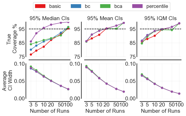
Bootstrap CIs for a real parameter are based on re-sampling with replacement from a fixed set of samples to create a bootstrap sample of size and compute the bootstrap parameter and repeating this process a numerous to create the bootstrap distribution over . In this paper, we evaluate the following non-parametric methods for constructing CIs for using this bootstrap distribution:
-
1.
Basic bootstrap, also known as the reverse percentile interval, uses the empirical quantiles from the bootstrap distribution of the parameter for defining the CI: , where denotes the percentile of the bootstrapped parameters and is the empirical estimate of the parameter based on finite samples.
-
2.
Percentile bootstrap. The percentile bootstrap proceeds in a similar way to the basic bootstrap, using percentiles of the bootstrap distribution, but with a different formula: for defining the CI.
-
3.
Bias-corrected (bc) bootstrap – adjusts for bias in the bootstrap distribution.
-
4.
Bias-corrected and accelerated (bca) bootstrap, by Efron [29], adjusts for both bias and skewness in the bootstrap distribution. This approach is typically considered to be more accurate and has better asymptotic properties. However, we find that it is not as effective as percentile methods in the few-run deep RL regime.
More technical details about bootstrap CIs can be found in [40]. We find that bootstrap CIs for mean scores per game (computed using random samples) require many more runs than aggregate scores (computed using random samples) for achieving true coverage close to the nominal coverage of 95% (c.f. Figure A.18 vs. Figure A.19).
Number of bootstrap re-samples. Unless specified otherwise, for computing uncertainty estimates using stratified bootstrap, we use 50,000 samples for aggregate metrics and 2000 samples for pointwise confidence bands and average probability of improvement. Using larger number of samples then the above specified values might result in more accurate uncertainty estimates but would be slower to compute.
Stratified bootstrap over tasks and runs111111Thanks to David Silver and Tom Schaul for suggesting stratified bootstrapping over tasks.. With access to only 1-2 runs per task, stratified bootstrapping can be done over tasks (Figure A.22), to answer the question: ‘‘If I repeat the experiment with a different set of tasks, what performance an algorithm is I expected to get?’’ It shows the sensitivity of the aggregate score to a given task and can also be viewed as an estimate of performance if we had used a larger unknown population of tasks [e.g., 94, 90]. Compared to the interval estimates in Figure 9, bootstraping over tasks results in much larger uncertainty due to high variations in performance across different tasks (e.g., easy vs hard exploration tasks).



A.6 Visualizing score distributions

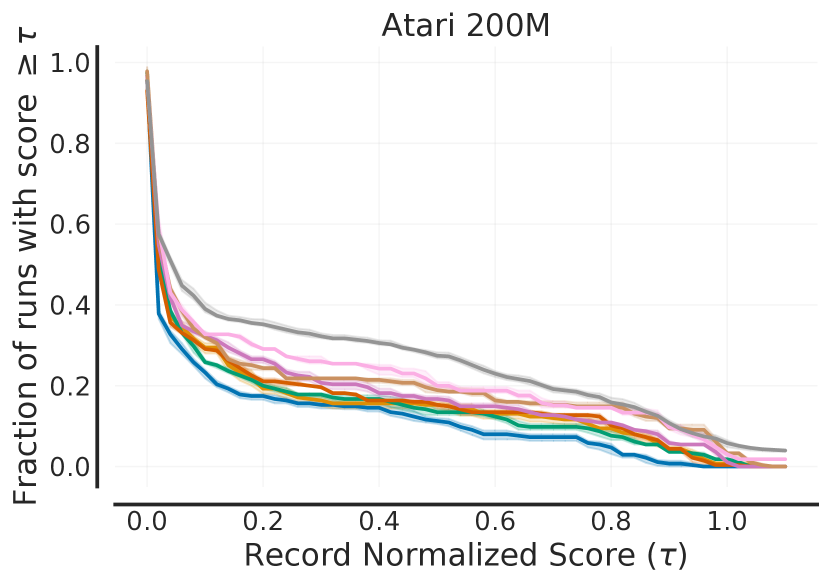
Choice of Normalization. We used existing normalization schemes which are prevalent on benchmarks including human normalized scores for Atari 100k and ALE, PPO normalized scores and Min-Max normalized scores for Procgen, and Min-Max Normalized scores (minimum scores set to zero) scores for DM Control. We do not use record normalized scores for ALE (Figure A.27) in the main text as ALE results are reported by evaluating agents for 30 minutes of game-play as opposed to record scores which were obtained using game play spanning numerous hours (e.g., Toromanoff et al. [105] recommend evaluating agents for 100 hours). Furthermore, we recommend using Min-Max Normalized scores for Procgen instead of PPO Normalized scores (Figure A.21) to allow for comparisons to methods which do not build upon PPO [92].
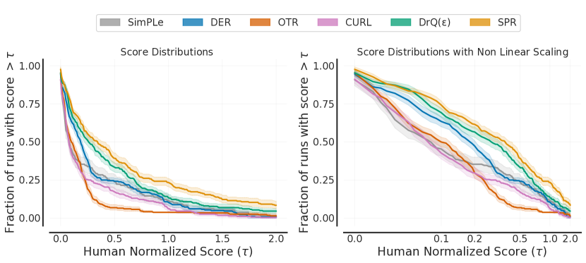
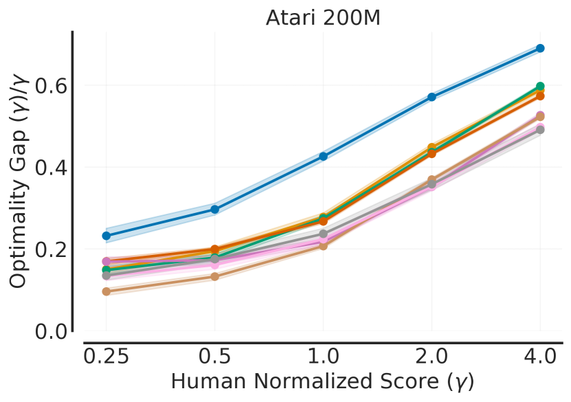
Scaling x-axis in score distributions. Figure A.23 (right) and Figure A.24 (right) shows an alternative for visualizing score distributions where we simply scale the -axis depending on the fraction of runs in a given region. This scaling more clearly shows the differences in algorithms by focusing on the regions where most of the runs lie121212Thanks to Mateo Hessel for suggesting this visualization scheme and the difficulty progress metric..
![[Uncaptioned image]](/html/2108.13264/assets/x34.png)
A.7 Aggregate metrics: Additional visualizations and details
Alternative aggregate metrics. Different aggregate metrics emphasize different characteristics and no single metric would be sufficient for evaluating progress. While score distributions provide a full picture of evaluation results, we provide suggestions for alternative aggregate metrics to highlight other important aspects of performance across different tasks and runs.
-
•
Difficulty Progress: One might be more interested in evaluating progress on the hardest tasks on a benchmark [3]. In addition to optimality gap which emphasizes all tasks below a certain performance level, a possible aggregate measure to consider is the mean scores of the bottom 25% of the runs (Figure A.25, left), which we call Difficulty Progress (DP-25).
- •
Choice of for optimality gap. When using min-max normalized scores or human-normalized scores, setting a score threshold of is sensible as it considers performance on games below maximum performance or human performance respectively. If there is no preference for a specific threshold, an alternative is to consider a curve of optimality gap as the threshold is varied, as shown in Figure A.27, which shows how far from optimality an algorithm is given any threshold -- a small value of optimality gaps for all achievable score thresholds is desirable.
Probability of improvement. To compute the probability of improvement for a task for algorithms and with and runs respectively, we use the Mann-Whitney U-statistic [71], that is,
| (A.2) |
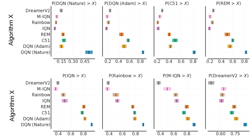
Please note that if the probability of improvement is higher than 0.5 and the CIs do not contain 0.5, then the results are statistically significant. Furthermore, if the upper CI is higher than a threshold of 0.75, then the results are said to be statistically meaningful as per the Neyman-Pearson statistical testing criterion by Bouthillier et al. [12]. We show the average probability of improvement metrics for Atari 100k and ALE in Figure A.29 and Figure A.28. These estimates show how likely an algorithm improves upon another algorithm.
Aggregate metrics on Atari 100k, Procgen and DM Control as well as ranking on individual tasks on DM Control are visualized in Figures A.30--A.33.
