A Case for Task Sampling based Learning for Cluster Job Scheduling
Abstract
The ability to accurately estimate job runtime properties allows a scheduler to effectively schedule jobs. State-of-the-art online cluster job schedulers use history-based learning, which uses past job execution information to estimate the runtime properties of newly arrived jobs. However, with fast-paced development in cluster technology (in both hardware and software) and changing user inputs, job runtime properties can change over time, which lead to inaccurate predictions.
In this paper, we explore the potential and limitation of real-time learning of job runtime properties, by proactively sampling and scheduling a small fraction of the tasks of each job. Such a task-sampling-based approach exploits the similarity among runtime properties of the tasks of the same job and is inherently immune to changing job behavior. Our analytical and experimental analysis of 3 production traces with different skew and job distribution shows that learning in space can be substantially more accurate. Our simulation and testbed evaluation on Azure of the two learning approaches anchored in a generic job scheduler using 3 production cluster job traces shows that despite its online overhead, learning in space reduces the average Job Completion Time (JCT) by 1.28, 1.56, and 1.32 compared to the prior-art history-based predictor. Finally, we show how the sampling-based learning can be extended to schedule DAG jobs and achieve similar speedups over the prior-art history-based predictor.
1 Introduction
In big-data compute clusters, jobs arrive online and compete to share the cluster resources. In order to best utilize the cluster and to ensure that jobs also meet their service level objectives, efficient scheduling is essential. However, as jobs arrive online, their runtime characteristics are not known a priori. Due to this lack of information, it is challenging for the cluster scheduler to determine the right job execution order that optimizes scheduling metrics such as maximal resource utilization or application service level objectives.
An effective way to tackle the challenges of cluster scheduling is to learn the runtime characteristics of pending jobs, which allows the scheduler to exploit offline scheduling algorithms that are known to be optimal, e.g., Shortest Job First (SJF) for minimizing the average completion time. Indeed, there has been a large amount of work [53, 45, 48, 27, 36, 44, 50, 56] on learning job runtime characteristics to facilitate cluster job scheduling.
In essence, all of the previous learning algorithms learn job runtime characteristics from observing historical executions of the same jobs, which execute the same code but process different sets of data, or of similar jobs, which have matching features such as the same application name, the same job name, or the same user who submitted the job.
The effectiveness of the above history-based learning schemes critically rely on two conditions to hold true: (1) The jobs are recurring; (2) The performance of the same or similar jobs will remain consistent over time.
In practice, however, the two conditions often do not hold true. First, many previous work have acknowledged that not all jobs are recurrent. For example, in the traces used in Corral [44] and Jockey [30], only 40% of the jobs are recurrent, and Morpheus [45] shows that only 60% of the jobs are recurrent. Second, even the authors of history-based prediction schemes such as 3Sigma [48] and Morpheus [45] strongly argued why runtime properties of jobs, even with the same input, will not remain consistent and will keep evolving. The primary reason is due to updates in cluster hardware, application software, and user scripts to execute the cluster jobs. Third, our own analysis of three production cluster traces (§4) have also shown that historical job runtime characteristics have considerable variations.
In this paper, we explore an alternative approach to learning runtime properties of distributed jobs online to facilitate cluster job scheduling. The approach is motivated by the following key observations about distributed jobs running on shared clusters: (1) a job typically has a spatial dimension, i.e., it typically consists of many tasks; and (2) the tasks (in the same phase) of a job typically execute the same code and process different chunks of similarly sized data [9, 16]. These observations suggest that if the scheduler first schedules a few sampled tasks of a job, known as pilot tasks, to run till finish, it can use the observed runtime properties of those tasks to accurately estimate those of the whole job. Effectively, such a task-sampling-based approach learns job properties in the spatial dimension. We denote the new learning scheme as SLearn, for “learning in space”.
Intuitively, by using the execution of pilot tasks to predict the properties of other tasks, SLearn avoids the primary drawback of history-based learning techniques, i.e., relying on jobs to be recurring and job properties to remain stationary over time. However, learning in space introduces two new challenges: (1) its estimation accuracy can be affected by the variations of task runtime properties, i.e., task skew; (2) delaying scheduling the remaining tasks of a job till the completion of sampled tasks may potentially hurt the job’s completion time.
In this paper, we perform a comprehensive comparative study of history-based learning (learning in time) and sampling-based learning (learning in space), to systematically answer the following questions: (1) Can learning in space be more accurate than learning in time? (2) If so, can delaying scheduling the remaining tasks of a job till the completion of sampled tasks be more than compensated by the improved accuracy and result in improved job performance, e.g., completion time?
We answer the first question via quantitative analysis, and trace and experimental analysis based on three production job traces, including two public cluster traces from Google released in 2011 and 2019 [8, 11] and a private trace from 2Sigma [1]. We answer the second question by designing a generic scheduler that schedules jobs based on job runtime estimates to optimize a given performance metric, e.g., average job completion time (JCT), and then plug into the scheduler different prediction schemes, in particular, learning in time and learning in space, to compare their effectiveness.
We summarize the major findings and contributions of this paper as follows:
-
•
Based on literature survey and analysis using three production cluster traces, we show that history is not a stable and accurate predictor for runtime characteristics of distributed jobs.
-
•
We propose SLearn, a novel learning approach that uses sampling in the spatial dimension of jobs to learn job runtime properties online. We also provide solutions to practical issues such as dealing with thin jobs (jobs with a few tasks only) and work conservation.
-
•
Via quantitative, trace and experimental analysis, we demonstrate that SLearn can predict job runtime properties with much higher accuracy than history-based schemes. For the 2Sigma, Google 2011, and Google 2019 cluster traces, the median prediction error are 18.98%, 13.68%, and 51.84% for SLearn but 36.57%, 21.39%, and 71.56% for the state-of-the-art history-based 3Sigma, respectively.
-
•
We show that learning job runtime properties by sampling job tasks, although delays scheduling the remaining tasks of a job, can be more than compensated by the improved accuracy, and as a result reduces the average JCT. In particular, our extensive simulations and testbed experiments using a prototype on a 150-node cluster in Microsoft Azure show that compared to the prior-art history-based predictor, SLearn reduces the average JCT by 1.28, 1.56, and 1.32 for the extracted 2Sigma, Google 2011 and Google 2019 traces, respectively.
-
•
We show how the sampling-based learning can be extended to schedule DAG jobs. Using a DAG trace generated from the Google 2019 trace, we show a hybrid sampling-based and history-based scheme reduces the average JCT by 1.25 over a pure history-based scheme.
2 Background and Related Work
In this section, we provide a brief background on the cluster scheduling problem, review existing learning-based schedulers, and discuss their weaknesses.
2.1 Cluster Scheduling Problem
In both public and private clouds, clusters are typically shared among multiple users to execute diverse jobs. Such jobs typically arrive online and compete for shared resources. In order to best utilize the cluster and to ensure that jobs also meet their service level objectives (SLOs), efficient job scheduling is essential. Since jobs arrive online, their runtime characteristics are not known a priori. This lack of information makes it challenging for the scheduler to determine the right order for running the jobs that maximizes resource utilization and/or meets application SLOs. Additionally, jobs have different SLOs. For some meeting deadlines is important while for others faster completion or minimizing the use of networks is more important. Such a diverse set of objectives pose further challenges to effective job scheduling [31, 30, 19, 44, 45, 57, 56].
2.2 Job Model
We consider big-data compute clusters running data-parallel frameworks such as Hadoop [4], Hive [6], Dryad [37], Scope [22], and Spark [7] that run simple MapReduce jobs [28] or more complex DAG-structured jobs, where each job processes a large amount of data. Each job consists of one or multiple stages, such as map or reduce, and each stage partitions the data into manageable chunks and runs many parallel tasks, each for processing one data chunk.
2.3 Existing Learning-based Schedulers
| Name | Property | Estimation | Learning |
| estimated | technique | frequency | |
| Corral | Job runtime | Offline model | On arrival |
| [44] | (not updated) | ||
| DCOSR | Memory elasti- | Offline model | Scheduler |
| [36] | city profile | (not updated) | dependent |
| Jockey | Job runtime | Offline | Periodic |
| [30] | simulator | ||
| 3Sigma | Job runtime | Offline | On arrival |
| [48] | history dist. | model |
An effective way to tackle the challenges of cluster scheduling is to learn runtime characteristics of pending jobs. As such cluster schedulers using various learning methods have been proposed [44, 45, 19, 48, 53, 36, 50, 21, 51, 25, 46]. In essence, all previous learning schemes are history-based, i.e., they learn job characteristics by observations made from the past job executions.111 Some recent work use the characteristics of completed mini-batches as a proxy for the remaining mini-batches, to improve the scheduling of ML jobs [55]. However, such jobs are different in that the mini-batches in general experience significantly less (task-level) variations than what we studied in this paper. In particular, existing learning approaches can be broadly categorized into the following groups, as summarized in Table 1.
Learning offline models.
Corral’s prediction model is designed with the primary assumptions that most jobs are recurring in nature, and the latency of each stage of a multi-stage job is proportional to the amount of data processed by it, which do not always hold true [44].
DCOSR [36] predicts the memory usage for data parallel compute jobs using an offline model built from a fixed number of profile runs that are specific to the framework and depend on the framework’s properties. Any software update in the existing frameworks, addition of new framework or hardware update will require an update in profile.
For analytics jobs that perform the same computation periodically on different sets of data, Tetris [32] takes measurements from past executions of a job to estimate the requirements for the current execution.
Learning offline models with periodic updates.
Jockey [30] periodically characterizes job progress at runtime, which along with a job’s current resource allocation is used by an offline simulator to estimate the job’s completion time and update the job’s resource allocation. Jockey relies on job recurrences and cannot work with new jobs.
Learning from similar jobs.
Instead of using execution history from the exact same jobs, JVuPredict [52] matches jobs on the basis of some common features such as application name, job name, the user who owns the job, and the resource requested by the job. 3Sigma [48] extends JVuPredict [52] by introducing a new idea on prediction: instead of using point metrics to predict runtimes, it uses full distributions of relevant runtime histories. However, since it is impractical to maintain precise distributions for each feature value, it resorts to approximating distributions, which compromises the benefits of having full distributions.
2.4 Learning from History: Assumptions and Reality
Predicting job runtime characteristics from history information relies on the following two conditions to hold, which we argue may not be applicable to modern day clusters.
Condition 1: The jobs are recurring.
Condition 2: The performance of the same or similar jobs will remain consistent over time.
Previous works [48, 45, 44, 30] that exploited history-based prediction have considered jobs in one of the following two categories. (1) Recurring jobs: A job is re-scheduled to run on newly arriving data; (2) Similar jobs: A job has not been seen before but has some attributes in common with some jobs executed in the past [52, 48]. Many of the history-based approaches only predict for recurring jobs [45, 44, 30], while some others [48, 52, 25, 46] work for both categories of jobs.
However, even the authors of history-based prediction schemes such as 3Sigma [48] and Morpheus [45] strongly argued why runtime properties of jobs, even with the same input, will keep evolving. The primary reason is that updates in cluster hardware, application software, and user scripts to execute the cluster jobs affect the job runtime characteristics. They found that in a large Microsoft production cluster, within a one-month period, applications corresponding to more than 50% of the recurring jobs were updated. The source code changed by at least 10% for applications corresponding to 15-20% of the jobs. Additionally, over a one-year period, the proportion of two different types of machines in the cluster changed from 80/20 to 55/45. For a same production Spark job, there is a 40% difference between the running time observed on the two types of machines [45].
For these reasons, although the state-of-the-art history-based system 3Sigma [48] uses sophisticated prediction techniques, the predicted running time for more than 23% of the jobs have at least 100% error, and for many the prediction is off by an order of magnitude.
3 SLearn – Learning in Space
In this paper, we explore an alternative approach to learning job runtime properties online in order to facilitate cluster job scheduling. The approach is motivated by the following key observations about distributed jobs running in shared clusters: (1) a distributed job has a spatial dimension, i.e., it typically consists of many tasks; (2) all the tasks in the same phase of a job typically execute the same code with the same settings [9, 16, 12], and differ in that they process different chunks of similarly sized data. Hence, it is likely that their runtime behavior will be statistically similar.
The above observations suggest that if the scheduler first schedules a few sampled tasks of a job to run till finish, it can use the observed runtime properties of those tasks to accurately estimate those of the whole job. In a modular design, such an online learning scheme can be decoupled from the cluster scheduler. In particular, upon a job arrival, the predictor first schedules sampled tasks of the job, called pilot tasks, till their completion, to learn the job runtime properties. The learned job properties are then fed into the cluster job scheduler, which can employ different scheduling polices to meet respective SLOs. Effectively, the new scheme learns job properties in the spatial dimension, i.e.,learning in space. We denote the new learning scheme as SLearn.
| Applicability | Adapti- | Accuracy | Runtime | |
| veness | overhead | |||
| Time | Recurring jobs | No/Yes | Depends | No |
| Space | New/Recurring jobs | Yes | Depends | Yes |
Table 2 summarizes the pros and cons of the two learning approaches along four dimensions: (1) Applicability: As discussed in §2.3, most history-based predictors cannot be used for the jobs of a new category or for categories for which the jobs are rarely executed. In contrast, learning in space has no such limitation; it can be applied to any new job. (2) Adaptiveness to change: Further, history-based predictors assume job runtime properties persist over time, which often does not hold, as discussed in §2.4. (3) Accuracy: The accuracy of the two approaches are directly affected by how they learn, i.e., in space versus in time. The accuracy of history-based approaches is affected by how stable the job runtime properties persist over time, while that of sampling-based approach is affected by the variation of the task runtime properties, i.e., the extent of task skew. (4) Runtime overhead: The history-based approach has an inherent advantage of having very low to zero runtime overhead. It performs offline analysis of historical data to generate a prediction model. In contrast, sampling-based predictors do not have offline cost, but need to first run a few pilot tasks till completion before scheduling the remaining tasks. This may potentially delay the execution of non-sampled tasks.
The above qualitative comparison of the two learning approaches raises the following two questions: (1) Can learning in space be more accurate than learning in time? (2) If so, can delaying scheduling the remaining tasks of a job till the completion of sampled tasks be more than compensated by the improved accuracy, so that the overall job performance, e.g., completion time, is improved? We answer the first question via analytical, trace and experimental analysis in §4 and the second question via a case study of cluster job scheduling using the two types of predictors in §5.
4 Accuracy Analysis
In this section, we perform an in-depth study of the prediction accuracy of the two learning approaches: learning in time (history-based learning) and learning in space (task-sampling-based learning). Both approaches can potentially be used to learn different job properties for different optimization objectives. In this paper, we focus on job completion time because it is an important metric that has been intensively studied in recent work [35, 36, 29, 24, 44, 48, 33, 23].
4.1 Analytical Comparison
We first present a theoretical analysis of the prediction accuracies of the two approaches. We caution that here we use a highly-stylized model (e.g., two jobs and normal task-length distributions), which does not capture the possible complexity in real clusters, such as heavy parallelism across servers and highly-skewed task-length distributions. Nonetheless, it reveals important insights that help us understand in which regimes history-based schemes or sampling-based schemes will perform better. Consider a simple case of two jobs and , where each job has tasks. The size of each task of is known. Without loss of generality, let us assume that the task size of is 1. Thus, the total size of is . The size of a task of is however unknown. Let denote the average task size of , and this its total size is . Clearly, if we knew precisely, then we should have scheduled first if and first if . However, suppose that we only know the following: (1) (Prior distribution:) follows a normal distribution with mean and variance ; (2) Given , the size of a random task of the job follows a normal distribution with mean and variance . Intuitively, captures the variation of mean task-lengths across many i.i.d. copies of job , i.e., job-wise variation, while captures the variation of task-lengths within a single run of job , i.e., task-wise variation. We note that the parameters and are not used by the predictors below.
Now, consider two options for estimating the mean task-length :1) A history-based approach (§4.1.1) and (2) a sampling-based approach where we sample tasks from (§4.1.2).
4.1.1 History-based Schemes
Since no samples of job are used, the best predictor for its mean task length is . In other words, the scheduling decision will be based on only. The difference between the true mean task length, x, and is simply captured by the job-wise variance .
4.1.2 Sampling-based Schemes
Suppose that we sample tasks from . Collect the sampled task lengths into a vector:
.
Then, based on our probabilistic model, we have
,
We are interested in an estimator of given . We have
,
where the last step follows from standard results on the posterior distribution with Gaussian priors (see, e.g., [18]). In other words, conditioned on , also follows a normal distribution with mean = and variance = .
Note that this represents the estimator quality using the information of both job-wise variations and task-wise variations. If the estimator is not informed of the job-wise variations, we can take , and the conditional distribution of given becomes normal with mean and variance .
From here we can draw the following conclusions. First, whether history-based schemes or sampling-based schemes have better prediction accuracy for an unknown job depends on the relationship between job-wise variations and the task-wise variation . If the job-wise variation is large but the task-wise variation is small, i.e., , then sampling-based schemes will have better prediction accuracy. Conversely, if the job-wise variation is small but the task-wise variation is large, i.e., , then history-based schemes will have better prediction accuracy. Second, while the accuracy of history-based schemes is fixed at , the accuracy of sampling-based schemes improves as increases. Thus, when we can afford the overhead of more samples, the sampling-based schemes become favorable. Our results from experimental data below will further confirm these intuitions.
| Trace | Arrival | Resource | Resource | Indiv. task |
| time | requested | usage | duration | |
| 2Sigma | Yes | Yes | No | Yes |
| Google 2011 | Yes | Yes | Yes | Yes |
| Google 2019 | Yes | Yes | Yes | Yes |
4.2 Trace-based Variability Analysis
Our theoretical analysis in §4.1 provides insights on how the prediction accuracies of the two approaches depend on the variation of job run times across time and space. To understand how such variations fare against each other in practice, we next measure the actual variations in three production cluster traces. Table 3 summarizes the information available in the traces that are used in our analysis.
Traces.
Our first trace is provided by 2Sigma [1]. The cluster uses an internal proprietary job scheduler running on top of a Mesos cluster manager [2]. This trace was collected over a period of 7 months, from January to July 2016, and from 441 machines and contains approximately 0.4 million jobs [17].
We also include two publicly available traces from Google released in May 2011 and May 2019 [8, 11], collected from 1 and 8 Borg [54] cells over periods of 29 and 31 days, respectively. The machines in the clusters are highly heterogeneous, belonging to at least three different platforms that use different micro-architectures and/or memory technologies [20]. Further, according to [9], the machines in the same platform can have substantially different clock rates, memory speed, and core counts. Since the original Google 2019 trace has data from 8 different cells located in 8 different locations, and given that we already have two other traces from the US, we chose the batch tier of Cluster G in the Google 2019 trace, which is located in Singapore [12], as our third trace to diversify our trace collection.
We calculate the variations in task runtimes for each job across time and across space as follows.
Variation across time.
To measure the variation in mean task runtime for a job across the history, we follow the following prediction mechanism defined in 3Sigma [48] to find similar jobs.
As discussed in §2.3, 3Sigma [48] uses multiple features to identify a job and predicts its runtime using the feature that gives the least prediction error in the past. We include all six features used in 3Sigma: application name, job name, user name (the owner of the job), job submission time (day and hour), and resources requested (cpu and memory) by the job.
For each feature, we define the set of similar jobs as all the jobs executed in the history window (defined below) that had the same feature value. Next, we calculate the average task runtime of each job in the set. Then, we calculate the Coefficient of Variation (CoV) of the average task runtimes across all the jobs in the set. We repeat the above process for all the features. We then compare the CoV values thus calculated and pick the minimum CoV. Effectively, the above procedure selects the least possible variation across history.
Varying the history length in prediction across time.
3Sigma used the entire history for prediction. Intuitively, the length of the history affects the trade-off between the number of similar jobs and the staleness of the history information. For this reason, we optimized 3Sigma by finding and using the history length that gives the least variation. Specifically, we define the length of history based on a window size , i.e., the number of past consecutive days. In our analysis below, we vary among 3, 7, and 14 for the three traces.
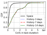
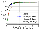
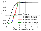
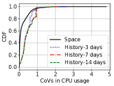
Variation across space.
To measure the extent of variation across space, we look at the CoV (CoV ) in the task runtimes within a job. As shown in §4.1, the variance in the task runtime predicted from sampling is , where is the variance in the runtimes across all the tasks within the job and is the number of tasks sampled. Thus, we first estimate from all tasks within the job. We then report the CoV of our task runtime prediction after sampling tasks as . Our complete scheduler design in §5.1 uses an adaptive sampling algorithm which mostly uses 3% for the three traces. Thus, for measuring the extent of variation across space here, we assume a 3% sampling ratio and plot .
Variability comparison.
For consistency, all analysis results here are for the same, shortest trace period that can be used for sliding-window-history based analysis, e.g., the last 15 days under the 14-day window for the 29-day Google 2011 trace. (The analysis then varies the length of the sliding window in history-based learning.) Figure 2 visualizes the two CoVs for each of 70 randomly selected jobs from the 2Sigma trace in the order of their arrival, also using the best window size of 14 days.

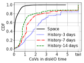
Fig. 1(a)–Fig. 1(c) show the CDFs of CoVs in task duration measured across space and across history for multiple history window sizes for the three traces. We see that in general using a shorter sliding window reduces the prediction error of 3Sigma, and the CoVs across tasks are moderately lower than the CoVs across history for the Google 2011 trace but significantly lower for 2Sigma and Google 2019 traces. For example, for the 2Sigma trace, the CoV across history is higher than the CoV across tasks for 85.40% of the jobs (not seen in Fig. 1(a) as jobs are ordered differently in different CDFs) and for more than 30% of the jobs, the CoV across history is at least 12.10 higher than the CoV across tasks.
Table 4 summarizes the results, where the CoVs across time correspond to the best history window size, i.e., 3 days for both Google traces and 14 days for the 2Sigma trace. As shown in the table, the P50 (P90) CoV across history are 1.00 (3.10) for the 2Sigma trace, 0.20 (0.73) for the Google 2011 trace, and 1.35 (1.67) for the Google 2019 trace. In contrast, the P50 (P90) CoV value across the task duration of the same set of jobs is much lower, 0.18 (0.55) for the 2Sigma trace, 0.04 (0.58) for the Google 2011 trace, and 0.70 (1.33) for the Google 2019 trace.
Fig. 1(d) and Fig. 1(e) further show the CDF of CoVs for CPU usage and Disk IO time for the Google 2011 trace (such resource usage is not available in the 2Sigma trace). The figures show that the variation in the values of these properties when sampled across space is also considerably lower compared to the variation observed over time.
| Trace | CoV over Time | CoV over Space | ||
| P50 | P90 | P50 | P90 | |
| 2Sigma | 1.00 | 3.10 | 0.18 | 0.55 |
| Google 2011 | 0.20 | 0.73 | 0.04 | 0.58 |
| Google 2019 | 1.35 | 1.67 | 0.70 | 1.33 |
4.3 Experimental Prediction Error Analysis
Recall from our analysis in §4.1 that lower task-wise variation than job-wise variation (§4.2) will translate into better prediction accuracy of sampling-based schemes over history-based schemes. While our analysis in §4.1 assumes normal distribution, we believe that a similar conclusion will hold in more general settings. To validate this, we next implement a sampling-based predictor SLearn, and experimentally compare it against a state-of-the-art history-based predictor 3Sigma [48] in estimating the job runtimes directly on production job traces.
Workload characteristics.
Since the three production traces described in §4.2 are too large, as in 3Sigma [48], we extracted smaller traces for experiments using the procedure described below.
Since the history-based predictor 3Sigma needs a history trace, we followed the same process as in [48] to extract the training trace for 3Sigma and the execution trace for all predictors, in three steps. (1) We divided each original trace in chronological order in two halves. (2) We compressed 2Sigma jobs to 150 tasks or fewer, by applying a compression ratio of original cluster size/150. Since the Google traces do not have many wide jobs yet the original clusters are very wide, with 12.5K machines, we dropped jobs with more than 150 tasks 222This is to avoid potential bias towards SLearn. A job with more than 150 tasks will have to be scheduled in more than one phase, which will be in favor of SLearn by diminishing the sampling overhead.. (3) We next selected the execution trace following the process below from the second half; these became 2STrace, GTrace11 and GTrace19, respectively. (4) We then selected jobs from the first half of each original trace that are feature-clustered with those jobs in the execution trace to form the "history" trace for 3Sigma.
We extracted the execution trace from each of the above-mentioned second halves by randomly selecting 1250 jobs with equal probability. Then, for each extracted trace, we adjust the arrival time of the jobs so that the average cluster load matches that in the original trace [17, 8, 11]. Table 5 summarizes the workload per window of the extracted traces, where a window is defined as a 1000-second interval sliding by 100 seconds at a time, and the load per window is the total runtime of all the jobs arrived in that window, normalized by the total number of CPUs in the cluster times the window length, i.e., 1000s. We see that for all three traces, the average system load is close to 1, though the load fluctuates over time, which is preserved by the random uniform job extraction.
| Trace | Average | P50 | P90 |
| 2STrace | 1.05 | 0.13 | 2.47 |
| GTrace11 | 1.01 | 0.29 | 1.49 |
| GTrace19 | 1.04 | 0.09 | 0.91 |
Prediction mechanisms and experimental setups.
We implement the 3Sigma predictor following its description in [48]. After learning the job runtime distribution (§4.2), it uses a utility function of the estimated job runtime associated with every job to derive its estimated runtime from the distribution, by integrating the utility function over the entire runtime distribution. Since our goal is to minimize the average JCT, we used a utility function that is inversely proportional to the square of runtime. We kept all the default settings we learned from the authors of 3Sigma [48].
As in §4.2, SLearn samples tasks per job, where is the number of tasks in the job. We only show the results for wide jobs (with 3 or more tasks) as in the complete SLearn design (§5.1.1), only wide jobs go through the sampling phase.
Results.
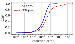
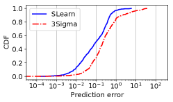
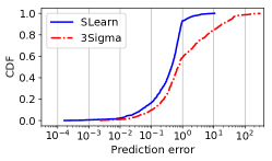
Fig. 3 shows the CDF of percentage error in the predicted job runtimes for the three traces. We see that SLearn has much better prediction accuracy than 3Sigma. For 2STrace, GTrace11, and GTrace19, the P50 prediction error are 18.30%, 9.15%, 21.39% for SLearn but 36.57%, 21.39%, 71.56% for 3Sigma, respectively, and the P90 prediction error are 58.66%, 49.95%, 92.25% for SLearn but 475.78%, 294.52%, 1927.51% for 3Sigma, respectively.
5 Integrating Sampling-based Learning with Job Scheduling: A Case Study
In this section, we answer the second key question about the sampling-based learning: Can delaying scheduling the remaining tasks till completing the sampled tasks be compensated by the improved prediction accuracy? We answer it through extensive simulation and testbed experiments.
Our approach is to design a generic scheduler, denoted as GS, that schedules jobs based on job runtime estimates to optimize a given performance metric, average job completion time (JCT). We then plug into GS different prediction schemes to compare their end-to-end performance.
5.1 Scheduler and Predictor Design
5.1.1 Generic Scheduler GS
GS replaces the scheduling component of a cluster manager like YARN [5]. The key scheduling objective of GS is to minimize the average JCT. Additionally, GS aims to avoid starvation.
The scheduling task in GS is divided into two phases, (1) job runtime estimation, and (2) efficient and starvation-free scheduling of jobs whose runtimes have been estimated. We focus here on the scheduling mechanism and discuss the different job runtime estimators in the following sections.
Inter-job scheduling.
Shortest job first (SJF) is known to be optimal in minimizing the average JCT when job execution depends on a single resource. Previous work has shown that scheduling distributed jobs even with prior knowledge is NP-hard (e.g., [24]), and an effective online heuristic is to order the distributed jobs based on each job’s total size [41, 42, 23, 40] [38]. In GS we use a similar heuristic; the jobs are ordered based on their total estimated runtime, i.e., .
Starvation avoidance.
SJF is known to cause starvation to long jobs. Hence, in GS we adopt a well-known multi-level priority queue structure to avoid job starvation [26, 49, 47, 23, 39]. Once GS receives the runtime estimates of a job, it assigns the job to a priority queue based on its runtime. Within a queue, we use FIFO to schedule jobs. Across the queues, we use weighted sharing of resources, where a priority queue receives a resource share according to its priority.
In particular, GS uses queues, to , with each queue having a lower queue threshold Q and a higher threshold Q for job runtimes. We set Q = 0, Q = , Q = Q. A queue with a lower index has a higher priority. GS uses exponentially growing queue thresholds, i.e., Q = E Q. To avoid any bias, we use the multiple priority queue structure with the same configuration when comparing different job runtime estimators.
Basic scheduling operation.
GS keeps track of resources being used by each priority queue. It offers the next available resource to a queue such that the weighted sharing of resources among the queues for starvation avoidance is maintained. Resources offered to a queue are always offered to the job at the head of the queue.
5.1.2 SLearn
To seamlessly integrate SLearn with GS, we need to use one of the priority queues for scheduling sampled tasks. We denote it as the sampling queue.
Fast sampling.
One design challenge is how to determine the priority for the sampling queue w.r.t. the other priority queues. On one hand, sampled tasks should be given high priority so that the job runtime estimation can finish quickly. On the other hand, the jobs whose runtimes have already been estimated should not be further delayed by learning new jobs. To balance the two factors, we use the second highest priority in GS as the sampling queue.
Handling thin jobs.
Recall that in SLearn, when a new job arrives, SLearn only schedules its pilot tasks, and delays other tasks until the pilot tasks finish and the job runtime is estimated. Such a design choice can inadvertently lead to higher JCTs for thin jobs, e.g., a two-task job would experience serialization of its two tasks. To avoid JCT degradations for thin jobs, we place a job directly in the highest priority queue if its width is under a threshold thinLimit.
Basic operations.
Upon the arrival of a new job, the cluster manager asynchronously communicates the job’s information to GS, which relays the information to SLearn. If the number of tasks in the job is under thinLimit, SLearn assigns it to the highest priority queue; otherwise, the job is assigned to the sampling queue, where a subset of its tasks (pilot tasks) will be scheduled to run. Once a job’s runtime is estimated from sampling, it is placed in the priority queue corresponding to its runtime estimate where the rest of its tasks will be scheduled.
How many and which pilot tasks to schedule?
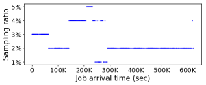
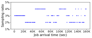
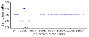
When a new job arrives, SLearn first needs to determine the number of pilot tasks. Sampling more tasks can give higher estimation accuracy, but also consumes more resources early on, which can potentially delay other jobs, if the job turns out to be a long job and should have been scheduled to run later under SJF. Further, we found the best sampling ratio appears to vary across difference traces. To balance the trade-off, we use an adaptive algorithm to dynamically determine the sampling ratio, as shown in Figure 4. The basic idea of the algorithm is to suggest a sampling ratio that has resulted in the lowest job completion time normalized by the job runtime based on the recent past. To achieve this, for every value in a defined range of possible sampling ratios (between 1% and 5%), it maintains a running score (), which is the average normalized JCT of recently finished jobs that used the corresponding sampling ratio. In practice we found a value of 100 works reasonably well. During system start-up, it tries sampling ratios of 2%, 3%, and 4% for the first jobs (Line 2–7). It further tries sampling ratios of 1% and 5% if going down from 3% to 2% or going up from 3% to 4% reduces the normalized JCT. Afterwards, for each new job, it uses the sampling ratio that has the lowest running score. Finally, upon each job completion, the score map is updated (Line 16–24).
Once the sampling ratio is chosen, SLearn selects pilot tasks for a job randomly.
How to estimate from sampled tasks?
Several methods such as bootstrapping, statistical mean or median can be used to predict job properties from sampled tasks. In GS, we use empirical mean to predict the mean task runtime.
Work conservation.
When the system load is low, some machines may be idle while the non-sampling tasks are waiting for the sampling tasks to finish. In such cases, SLearn schedules non-sampling tasks of jobs to run on otherwise idle machines. In work conservation, the jobs are scheduled in the FIFO order of their arrival.
1:procedure GetCurrentSamplingPercentage(Job j) 2: if j in First jobs then 3: return 3 4: else if j in Second jobs then 5: return 2 6: else if j in Third jobs then 7: return 4 8: minScore = getMinValue(srScoreMap) 9: if minScore.SR == 2 then 10: if 1.1*minScore.value < srScoreMap[3].value then 11: return 1 12: if minScore.SR == 4 then 13: if srScoreMap[3].value > 1.1*minScore.value then 14: return 5 15: return minScore.SR 16:procedure UpdateScoreOnJobCompletion(Job j) 17: sr = j.sr Get j’s sampling ratio. 18: normalizedJCT = j.jct Get j’s normalized JCT. 19: UpdateScoresMap(sr, normalizedJCT) 20:procedure UpdateScoreMaps(sr, normalizedJCT) 21: if Len(jobWiseSrScoresMap[sr])> then 22: Drop first element of jobWiseSrScoresMap[sr] 23: jobWiseSrScoresMap[sr].append(normalizedJCT) 24: srScoreMap[sr].value = mean(jobWiseSrScoresMap[sr])
5.1.3 Baseline Predictors and Policies
We compare SLearn’s effectiveness against four different baseline predictors and two policies: (1) 3Sigma: as discussed in §4.3. (2) 3SigmaTL: same as 3Sigma but handles thin jobs in the same way as SLearn; they are directly placed in the highest priority queue. This is to isolate the effect of thin job handling. (3) Point-Est: same as 3Sigma, with the only difference being that, instead of integrating a utility function over the entire runtime history, it predicts a point estimate (median in our case) from the history. (4) LAS: The Least Attained Service [49] policy approximates SJF online without explicitly learning job sizes, and is most recently implemented in the Kairos [29] scheduler. LAS uses multiple priority queues and the priority is inversely proportional to the service attained so far, i.e., the total execution time so far. We use the sum of all the task execution time to be consistent with all the other schemes. (5) FIFO: The FIFO policy in YARN simply prioritizes jobs in the order of their arrival. Since FIFO is a starvation free policy, there is no need for multiple priority queues. (6) Oracle: Oracle is an ideal predictor that always predicts with 100% accuracy.
5.2 Experimental Results
We evaluated SLearn’s performance against the six baseline schemes discussed above by plugging them in GS and execute the 3 traces (2STrace, GTrace11, and GTrace19) using large scale simulations and on a 150-node testbed cluster in Azure (§5.2.6).
5.2.1 Experimental Setup
Cluster setup.
We implemented GS, SLearn and baseline estimators with 11 KLOC of Java and python2. We used an open source java patch for Gridmix [15] and open source java implementation of NumericHistogram [13] for Hadoop. We used some parts from DSS, an open source job scheduling simulator [10], in simulation experiments.
We implemented a proxy scheduler wrapper that plugs into the resource manager of YARN [5] and conducted real cluster experiments on a 150-node cluster in MS Azure [14].
Following the methodology in recent work on cluster job scheduling [48, 52, 25], we implemented a synthetic generator based on the Gridmix implementation to replay jobs that follow the arrival time and task runtime from the input trace. The Yarn master runs on a standard DS15 v2 server with 20-core 2.4 GHz Intel Xeon E5-2673 v3 (Haswell) processor and 140GB memory, andthe slaves run on D2v2 with the same processor with 2-core and 7GB memory.
Parameters.
The default parameters for priority queues in GS in the experiments are: starting queue threshold () is ms, exponential threshold growth factor () is 10, number of queues () is set to 10, and the weights for time sharing assigned to individual priority queues decrease exponentially by a factor of 10. Previous work (e.g., [23]) and our own evaluation have shown that the scheduling results are fairly insensitive to these configuration parameters. We omit their sensitivity study here due to page limit. SLearn chooses the number of pilot tasks for wide jobs using the adaptive algorithm described in §5.1.2 and the threshold for thin jobs is set to 3. We evaluate the effectiveness of adaptive sampling in §5.2.2 and the sensitivity to thinLimit in §5.2.8.
Performance metrics.
We measure three performance metrics in the evaluation: JCT speedup, defined as the ratio of a JCT under a baseline scheme over under SLearn, the job runtime estimation accuracy, and job waiting time.
Workload.
We used the same training data for history-based estimators and the test traces (2STrace, GTrace11 and GTrace19) as described in §4.3.
5.2.2 Effectiveness of Adaptive Sampling
| Fraction of tasks chosen as pilot tasks | |||||||
| 1% | 2% | 3% | 4% | 5% | 10% | Adap. | |
| 2STrace | |||||||
| P50 pred. error (%) | 19.4 | 19.0 | 19.0 | 18.7 | 18.4 | 16.9 | 19.0 |
| Avg. JCT speedup () | 1.24 | 1.23 | 1.27 | 1.26 | 1.27 | 1.28 | 1.28 |
| P50 speedup () | 0.93 | 0.92 | 0.93 | 0.92 | 0.93 | 0.91 | 0.92 |
| GTrace11 | |||||||
| P50 pred. error (%) | 14.4 | 14.0 | 13.6 | 13.1 | 12.7 | 9.09 | 13.7 |
| Avg. JCT speedup () | 1.52 | 1.55 | 1.54 | 1.56 | 1.58 | 1.51 | 1.56 |
| P50 speedup () | 1.00 | 1.00 | 1.00 | 1.00 | 1.00 | 1.00 | 1.00 |
| GTrace19 | |||||||
| P50 pred. error (%) | 55.7 | 53.8 | 47.1 | 46.5 | 42.1 | 36.1 | 51.8 |
| Avg. JCT speedup () | 1.31 | 1.31 | 1.31 | 1.32 | 1.28 | 1.24 | 1.32 |
| P50 speedup () | 1.07 | 1.07 | 1.05 | 1.05 | 1.01 | 1.00 | 1.07 |
In this experiment, we evaluate the effectiveness of our adaptive algorithm for task sampling. Fig. 5 shows how the sampling ratio selected by the adaptive algorithm for each job varies between 1% and 5% over the duration of the three traces. We further compare average JCT speedup and P50 speedup under the adaptive algorithm with those under a fixed sampling ratio, ranging between 1% and 10%. Table 6 shows that the adaptive sampling algorithm leads to the best speedups for 2STrace and GTrace19 and is about only 1% worse than the best for GTrace11. Interestingly, we observe that no single sampling ratio works the best for all traces. Nonetheless, the adaptive algorithm always chooses one that is the best or closest to the best in terms of JCT speedup. More importantly, we see that the adaptive algorithm does not always use the sampling ratio with the best prediction accuracy, which shows that it effectively balances the tradeoff between prediction accuracy and sampling overhead.
5.2.3 Prediction Accuracy
SLearn achieves more accurate estimation of job runtime over 3Sigma – the details were already discussed in §4.3.
5.2.4 Average JCT Improvement
We now compare the JCT speedups achieved using SLearn over using the five baseline schemes defined in §5.1.3.
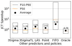
Fig. 6(a) shows the results for 2STrace. We make the following observations. (1) Compared to Oracle, SLearn achieves an average and P50 speedups of 0.79 and 0.73, respectively. This is because SLearn has some estimation error; it places 10.91% of wide jobs in the wrong queues, 3.54% in lower queues and 7.37% in higher queues. (2) SLearn improves the average JCT over 3Sigma by 1.28. This significant improvement of SLearn comes from much higher prediction accuracy compared to 3Sigma (Fig. 3). (3) The improvement of SLearn over 3SigmaTL, 1.26, is similar to that over 3Sigma, confirming thin job handling only played a small role in the performance difference of the two schemes. To illustrate SLearn’s high prediction accuracy, we show in Table 7 the fraction of wide jobs that were placed in correct queues by SLearn and 3Sigma. We observe that SLearn consistently assigns more wide jobs to correct queues than 3Sigma for all three traces. (4) Compared to Point-Est, SLearn improves the average JCT by 1.42. Again, this is because SLearn estimates runtimes with higher accuracy. (5) Compared to LAS, SLearn achieves an average JCT speedup of 1.91 and P50 speedup of 1.29. This is because LAS pays a heavy penalty in identifying the correct queues of jobs by moving them across the queues incrementally. (6) Lastly, compared with FIFO, SLearn achieves an average JCT speedup of 3.29 and P50 speedup of 8.45.
| Prediction | SLearn | 3Sigma |
| Technique | ||
| 2STrace | 89.09% | 73.84% |
| GTrace11 | 86.45% | 76.20% |
| GTrace19 | 73.96% | 58.07% |
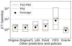
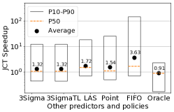
Fig. 6(b) shows the results for GTrace11. Scheduling under SLearn again outperforms all other schemes. In particular, using SLearn improves the average JCT by 1.56 compared to using 3Sigma, 1.55 compared to using 3SigmaTL, 2.17 compared to using Point-Est, and 1.65 compared to using the LAS policy. Fig. 6(c) shows that scheduling under SLearn outperforms all other schemes for GTrace19 too. In particular, using SLearn improves the average JCT by 1.32, 1.32, 1.54, and 1.72 compared to using 3Sigma, 3SigmaTL, Point-Est and the LAS policy, respectively.
In summary, our results above show that SLearn’s higher estimation accuracy outweighs its runtime overhead from sampling, and as a result achieves much lower average job completion time than history-based predictors and the LAS policy for the three production workloads.
5.2.5 Impact of Sampling on Job Waiting Time
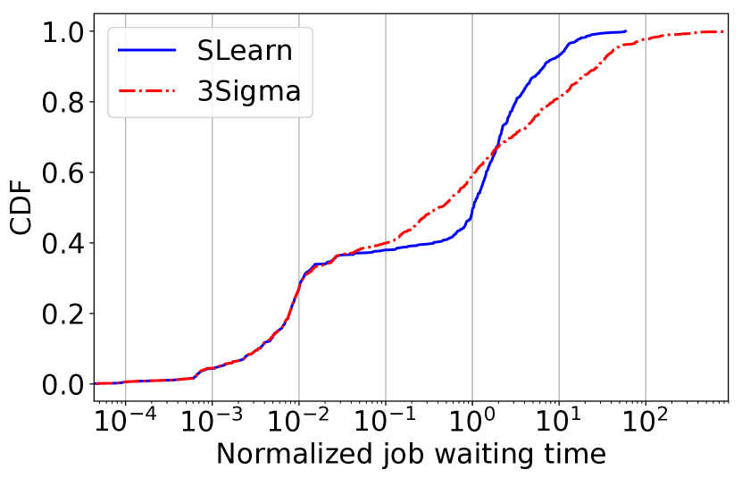
To gain insight into why sampling pilot tasks first under SLearn does not hurt the overall average JCT, we next compare the normalized waiting time of jobs, calculated as the average waiting time of its tasks under the respective scheme, divided by the mean task length of the job.
Fig. 7 shows the CDF of the normalized job waiting time under SLearn and 3Sigma. We see that the CDF curves can be divided into three segments. (1) The first segment, where both SLearn and 3Sigma have normalized waiting time (NWT) less than 0.04, covers 36.58% of the jobs, and 35.57% of the jobs are common. The jobs have almost identical NWT, much lower than 1 under both schemes. This happens because during low system load periods, e.g., lower than 1, the scheduler will schedule all the tasks to run under both scheme; under SLearn it schedules non-sampled tasks of jobs to run before their sampled tasks complete due to work conservation. (2) The second segment, where both schemes have NWT between 0.04 and 1.90, covers 30.51% of the jobs, and 20.38% of the jobs are common. Out of these 20.38%, 29.81% have lower NWT under SLearn and 70.19% have lower NWT under 3Sigma. This happens because when the system load is moderate, the jobs experience longer waiting time under SLearn than under 3Sigma because of sampling delay. (3) The third segment, where both schemes have NWT above 1.90, cover 32.91% of the jobs, and 24.68% of jobs are common. Out of these 24.68%, 83.08% have lower waiting time under SLearn and 16.92% under 3Sigma. This happens because when the system load is relatively high, although jobs incur the sampling delay under SLearn, they also experience queuing delay under 3Sigma, and the more accurate prediction of SLearn allows them to be scheduled following Shortest Job First more closely than under 3Sigma.
A detailed analysis of how the system load of the trace affects the relative job performance under the two predictors can be found in the Appendix.
5.2.6 Testbed Experiments
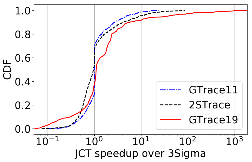
We next perform end-to-end evaluation of SLearn and 3Sigma on our 150-node Azure cluster. Fig. 8 shows the CDF of JCT speedups using SLearn over 3Sigma using 2STrace, GTrace11 and GTrace19. SLearn’s performance on the testbed is similar to that observed in the simulation. In particular, SLearn achieves average JCT speedups of 1.33, 1.46, and 1.25 over 3Sigma for the 2STrace, GTrace11, and GTrace19 traces, respectively.
5.2.7 Binning Analysis
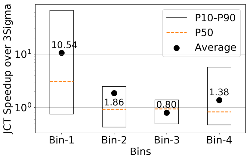
To gain insight into how different jobs are affected by SLearn over 3Sigma, we divide the jobs into four bins in Table 8 for 2STrace and show the JCT speedups for each bin in Fig. 9. The results for the other two traces are similar and are omitted due to page limit.
| width 3 (thin) | width 3 (wide) | |
| size (sm) | bin-1 (4.55%, 0.01%) | bin-2 (28.73%, 0.06%) |
| size (lg) | bin-3 (14.29%, 5.41%) | bin-4 (52.43%, 94.52%) |
We make the following observations. (1) SLearn improves the JCT for 82.46% of the jobs in Bin-1 and the average JCT speedup for the bin is 10.54. This happens because the jobs in this bin are thin and hence SLearn assigns them high priorities, which is also the right thing to do since these jobs are also small. (2) For bin-2, SLearn achieves an average JCT speedup of 1.86 from better prediction accuracy of SLearn. The speedups are lower than for Bin-1 as the jobs have to undergo sampling. However, Bin-1 and Bin-2 make up only 0.01% and 0.06% of the total job runtime and thus have little impact on the overall JCT. (3) Bin-3, which has 14.29% of the jobs and accounts for 5.41% of the total job size, has a slowdown of 20.00%. The main reason is that SLearn treats thin jobs in the FIFO order, whereas 3Sigma schedules them based on predicted sizes. (4) Bin-4, which accounts for a majority of the job and total job size, has an average speedup of 1.38, which contributes to the overall speedup of 1.28. The job speedups come from more accurate job runtime estimation of SLearn over 3Sigma. Finally, we note that while for the 2Sigma trace, the majority of thin jobs are large, for the Google 2011 (Google 2019) trace, only 1.90% (1.60%) of the total number of jobs are thin and large and they make up only 0.5% (0.5%) of the total job runtime..
5.2.8 Sensitivity to Thin Job Bypass
Finally, we evaluate SLearn’s sensitivity to thinLimt. Table 9 shows that for GTrace11 and GTrace19, the average JCT speedup barely varies with thinLimit, but for 2STrace, there is a big dip when increasing thinLimit to 4 or 5. This is because a significant number of jobs in 2STrace have width 4, which causes the number of thin jobs to increase from 18.84% to 58.50% when increasing thinLimit from 4 to 5.
| thinLimit | 2 | 3 | 4 | 5 | 6 |
| 2STrace | 1.23x | 1.28x | 1.14x | 0.97x | 0.84x |
| GTrace11 | 1.54x | 1.56x | 1.55x | 1.54x | 1.53x |
| GTrace19 | 1.33x | 1.32x | 1.32x | 1.30x | 1.29x |
6 Scheduling for DAG Jobs
In earlier sections, we have focused on the benefits of sampling-based prediction. On the other hand, we envision that there are situations where it would be beneficial to combine sampling-based and history-based predictions. Below, we present our preliminary work applying such a hybrid strategy for scheduling DAG jobs. We will discuss several other use cases of a hybrid strategy in §7. Note that for multi-phase DAG jobs, simply applying sampling-based prediction to each phase in turn cannot estimate the whole DAG runtime ahead of time. Instead, our hybrid design below aims to learn the runtime properties and optimize the performance of a multi-phase DAG job as a whole (e.g., [30, 33]).
Hybrid learning for DAGs (SLearn-DAG).
The key idea of SLearn-DAG is to adjust history-based prediction of the runtime of DAG jobs using sampling-based learning of its first stage. Upon arrival of a new DAG job, we estimate the runtime of its first stage using sampling-based prediction as described in §5.1.2, denoted as . We also estimate the duration of this stage using history-base 3Sigma, denoted as , and compute the adjustment ratio of . For each of the remaining stages of the DAG, we predict their runtime using 3Sigma and then multiply it with the adjustment ratio. In a nutshell, this hybrid design reduces the error of history-based prediction due to staleness of the learning data, while avoiding the delay of sampling across all other stages.
History-based learning for DAGs (3Sigma-DAG).
This is a straight-forward extension of 3Sigma. Upon arrival of a DAG job, it predicts independently the runtime for each stage using the 3Sigma and sums up the estimated runtime of all stages as the estimated runtime of the entire DAG.
We similarly extended other baselines described in §5.1.3 for DAG job.
Experimental setup.
We evaluated SLearn-DAG against 3Sigma-DAG by replaying cluster trace in simulation experiments based on GS (§5.1.1). We kept the simulation setup and parameters the same as used in the other experiments. In particular, a DAG is placed in the corresponding priority queue based on its estimated total runtime.
DAG Traces.
The only publically available DAG trace we could find is a trace from Alibaba[3], which could not be used as it does not contain features required for history-based prediction using 3Sigma. Instead, we followed the ideas in previous work, e.g., Branch Scheduling [34], to generate a synthetic DAG trace of about 900 jobs using the Google 2019 trace [11], denoted as GTrace19-DAG. The number of stages in DAGs in the GTrace19-DAG was randomly choosen to be between 2-5 and each stage is a complete job from the Google 2019 trace. The jobs that are part of the same DAG have the same jobname and the same username.
Results.
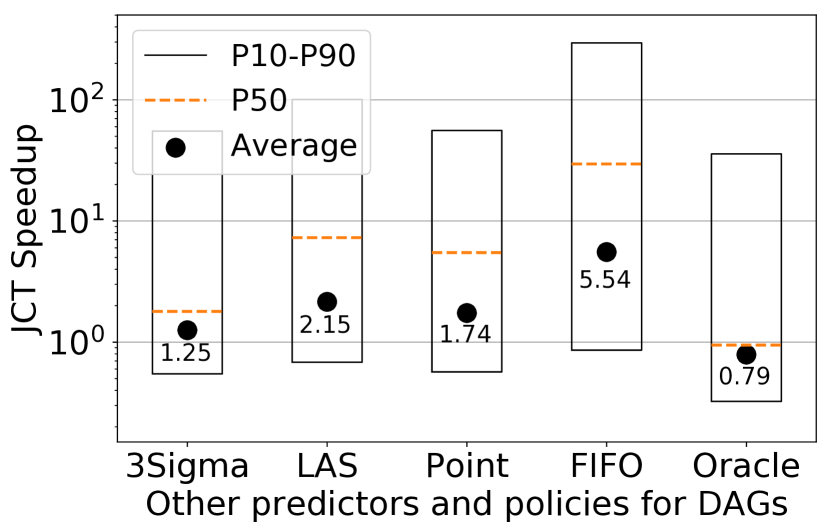
The results in Fig. 10 show that SLearn-DAG achieves significant speedup over other designs. The speedup is 1.26 over 3Sigma-DAG, 2.15 over LAS-DAG, and 1.74 over Point-Est-DAG. Looking deeper, we find that our sampling-based prediction still yields higher prediction accuracy: the P50 prediction error is 33.90% for SLearn-DAG, compared to 47.21% for 3Sigma-DAG. On the other hand, for DAG jobs the relative overhead of sampling (e.g, the delay) is lower since only the first stage is sampled. Together, they produce speedup comparable to earlier sections.
7 Discussions and Future Work
Combining history and sampling.
In addition to improving the scheduling of DAG jobs (§6), we discuss several additional motivations for combining history- and sampling-based learning. (1) For workloads with both recurring and first-time jobs, sampling-based learning can be used to estimate properties for first-time jobs, while history-based learning can be used for recurring jobs. (2) When the workload has both thin and wide jobs, history-based learning can be used for estimating the runtime for thin jobs, while sampling-based learning is used for wide jobs. (3) History-based learning can be used to establish a prior distribution, and sampling-based approach can be used to refine the posterior distribution. Such a combination is potentially more accurate than using either approach alone. For example, knowing the prior distribution of task lengths can help to develop better max task-length predictors, which can be useful for jobs with deadlines. (4) Though not seen in the production traces used in our study, in cases when task-wise variation and job-wise variation fluctuate, adaptively switching between the two prediction schemes may also help. (5) When the cluster is heterogeneous, an error adjustment using history, similar to what we did in §6, can be applied.
Dynamic adjustment of ThinLimit.
ThinLimit is a subjective threshold. It helps in segregating jobs for which waiting time due to sampling overshadows the improvement in prediction accuracy. The optimal choice of this limit will depend on the cluster load at the moment and hence can be adaptively chosen like the sampling percentage (Fig. 4 on page 4).
Heterogeneous clusters.
Extending sampling-based learning to heterogeneous clusters requires adjusting the task sampling process. One idea is to schedule pilot tasks on homogeneous servers and then scale their runtime to different types of servers using the ratio of machine speeds.
8 Conclusions
In this paper, we performed a comparative study of task-sampling-based prediction and history-based prediction commonly used in the current cluster job schedulers. Our study answers two key questions: (1) Via quantitative, trace and experimental analysis, we showed that the task-sampling-based approach can predict job runtime properties with much higher accuracy than history-based schemes. (2) Via extensive simulations and testbed experiments of a generic cluster job scheduler, we showed that although sampling-based learning delays non-sampled tasks till completion of sampled tasks, such delay can be more than compensated by the improved accuracy over the prior-art history-based predictor, and as a result reduces the average JCT by 1.28, 1.56, and 1.32 for three production cluster traces. These results suggest task-sampling-based prediction offers a promising alternative to the history-based prediction in facilitating cluster job scheduling.
Acknowledgement
We thank our shepherd Sangeetha Abdu Jyothi and the anonymous reviewers for their helpful comments. This work was supported in part by NSF grant 2113893.
Appendix: How does the system load affect the speedups of SLearn over 3Sigma?
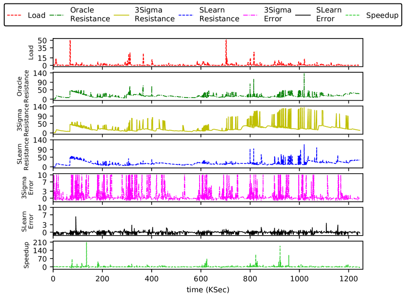
In this section, we provide an intuitive explanation for SLearn’s JCT speedup over 3Sigma in Section 5.2.4 for 2STrace in Figure 5(a). Figure 11 shows seven timeline values comparing SLearn and 3Sigma for the 2STrace as follows:
-
•
The top curve shows the total workload arrived in the past 1000 seconds, in terms of execution duration. The values are plotted in steps of 1000 seconds along the x-axis. A unit along the y-axis corresponds to the workload that needs 1000 seconds of the entire cluster’s compute capacity. Thus a workload of 1 in steady state implies no queue build-up under 100% utilization of the whole cluster.
-
•
The next three curves show the resistance faced by newly arrived jobs under Oracle, 3Sigma and SLearn, respectively, where resistance for a job is defined as the amount of higher priority workload existing at the time of its arrival, including the remaining duration of the already scheduled tasks. A unit along the y-axis for these curves also corresponds to the workload that needs 1000 seconds of the entire cluster’s compute capacity. For wide jobs (i.e., with 3 or more tasks), under SLearn we show the resistance value corresponding to the moment when the job’s size estimation is over and it has been placed in its estimated priority queue. The resistance values are plotted along the x-axis corresponding to each job’s arrival time.
-
•
The next two curves correspond to the percentage prediction error in 3Sigma and SLearn, respectively. They show signed error which are capped at 1000, e.g., a value of -20 on error curves means the job was estimated to be 20% smaller and a value of 1000 means job was estimated at least 1000% larger. The values are plotted along the x-axis corresponding to each job’s arrival time.
-
•
The bottom curve shows the job speedup (positive values) or slowdown (negative values) of SLearn compared to 3Sigma, plotted along the x-axis corresponding to each job’s arrival time. Thus all values are either above 1, showing the speedups of jobs under SLearn over under 3Sigma, or below -1, showing the speedups of jobs under 3Sigma over under SLearn.
With the above definitions of the curves, we next discuss how these curves in Fig. 11 demonstrate provides insights to when and why SLearn outperforms 3Sigma.
| Overestim- | Misplaced | Slowed | Average (P50) | Underesti- | Misplaced | Speedup | Average (P50) | |
| ated jobs | overestimated | misplaced | Positive error | mated jobs | underestimated | misplaced | Negative error | |
| jobs | jobs | jobs | jobs | |||||
| 3Sigma | 59.78% | 17.50% | 12.19% | 898.5% (48.00)% | 40.22% | 8.65% | 6.88% | -37.0% (-28.57)% |
| SLearn | 43.75% | 3.54 % | 2.85% | 30.65% (18.19)% | 55.45% | 7.37% | 3.64% | -26.79% (-20.69)% |
-
•
The speedup curve (bottom) shows the speedup under SLearn over under 3Sigma happens when the workload is high, e.g., between 600s and 620s, and 800s to 840s. Conversely, when the workload is below 1, e.g., between 400 and 600s, the two scheme perform similarly and there is no speedup of either scheme. In such cases, task sampling SLearn did not hurt jobs because non-sampled tasks did not have to wait for completion of sampled tasks due to work conservation (§5.1.2).
-
•
Intuitively, under any scheme, a job’s completion time is roughly proportional to its own total runtime (which is independent of the scheduling) plus the resistance it sees upon arrival, because the resistance value indicates the amount of workload that needs to be scheduled before the arriving job gets to run.
-
•
The resistance value, in turn, depends on the recently arrived workload and the prediction error and hence the scheduling decision for them.
-
•
First, if more workload has arrived in the recent past, it is likely that a newly arrived job will face higher resistance. This is shown by the strong correlation between the load curve and the Oracle resistance curve.
-
•
Second, high runtime prediction error can lead to high resistance. When the job runtime is estimated by the predictor to be larger than its actual size, it may be misplaced in a lower priority queue. If the error is more than 1000% then the job will definitely be placed in a lower priority queue. In such cases, the job will likely face higher resistance than it would have with accurate estimation. Conversely, when the job runtime is underestimated, it may be placed in a higher priority queue. Though such a job will finish faster than otherwise, it will create more resistance for other jobs that are actually smaller than it and thus slow them down.
-
•
The above impact of prediction error on resistance can be seen in Fig. 11. Since the prediction accuracy of SLearn is high, it has less impact on the resistance and as a result its resistance (fourth curve) is very similar to that of Oracle (second curve) 333We note that there can be some exceptions where jobs face lower resistance under SLearn compared to under Oracle, e.g., between time 200 - 400 KSec in Fig. 11. This happens because of mis-prediction in SLearn, e.g., when it underestimates the runtime of some jobs and places them in lower priority queues than otherwise, the subsequently arriving job will experience lower resistance. . In contrast, the resistance curve for 3Sigma (third curve) has many spikes, e.g., between 800s and 1050s, which happen when the workload (top curve) is high and it has high positive prediction error (fifth curve).
-
•
Finally, we can see that where ever there is higher resistance under 3Sigma (third curve) compared to under SLearn (fourth curve), e.g., between 800s and 1000s, jobs experience speedups under SLearn over under 3Sigma.
While the above explanation using Fig. 11 is based on the performance of SLearn and 3Sigma relative to that of Oracle, Table 10 gives a direct comparison of the scheduling behavior of the jobs under the two schemes in terms of runtime overestimation/underestimation, prediction error, and the resulting misplacement to the priority queues. We see that a larger number jobs are misplaced under 3Sigma compared to SLearn which led to the overall lower performance under 3Sigma.
In summary, whether a job finishes faster under SLearn compared to 3Sigma depends on two factors: the recent workload and the runtime prediction error. Due to higher prediction error of 3Sigma compared to SLearn, during high workload, jobs are more likely to be misplaced to the priorty queues and hence face higher resistance, which results in longer average completion time under 3Sigma.
References
- [1] 2sigma hedge fund. www.twosigma.com.
- [2] 2sigma’s proprietary job scheduler. https://www.twosigma.com/insights/article/cook-a-fair-preemptive-resource-scheduler-for-compute-clusters/.
- [3] Alibaba cluster trace. https://github.com/alibaba/clusterdata.
- [4] Apache hadoop. http://hadoop.apache.org.
- [5] Apache hadoop yarn. https://hadoop.apache.org/docs/current/hadoop-yarn/hadoop-yarn-site/YARN.html.
- [6] Apache hive. http://hive.apache.org.
- [7] Apache spark. http://spark.apache.org.
- [8] Cluster trace from google - 2011. https://github.com/google/cluster-data/blob/master/ClusterData2011_2.md.
- [9] A document released by google containing schema and details of the cluster trace released by google. https://drive.google.com/open?id=0B5g07T _gRDg9Z0lsSTEtTWtpOW8.
- [10] Dss scheduler. https://github.com/epfl-labos/DSS.
- [11] Google cluster-usage traces, retrieved 21st july 2020. https://research.google/tools/datasets/google-cluster-workload-traces-2019/.
- [12] Google cluster-usage traces, retrieved 21st july 2020. https://drive.google.com/file/d/ 10r6cnJ5cJ89fPWCgj7j4LtLBqYN9RiI9/view.
- [13] Hadoop patch for numeric histogram. https://issues.apache.org/jira/browse/YARN-2672.
- [14] Microsoft azure. http://azure.microsoft.com.
- [15] A patch for gridmix. https://issues.apache.org/jira/browse/YARN-2672.
- [16] Personal communication with a 2sigma engineer regarding properties of the 2sigma trace used.
- [17] A private trace collected by 2sigma engineers from their clusters. www.twosigma.com.
- [18] Resutls on the posteriro distribution with gaussian priors. https://people.eecs.berkeley.edu/ jordan/courses/260-spring10/lectures/lecture5.pdf.
- [19] Faraz Ahmad, Srimat T. Chakradhar, Anand Raghunathan, and T. N. Vijaykumar. Shufflewatcher: Shuffle-aware scheduling in multi-tenant mapreduce clusters. In 2014 USENIX Annual Technical Conference (USENIX ATC 14), pages 1–13, Philadelphia, PA, 2014. USENIX Association.
- [20] George Amvrosiadis, Jun Woo Park, Gregory R. Ganger, Garth A. Gibson, Elisabeth Baseman, and Nathan DeBardeleben. On the diversity of cluster workloads and its impact on research results. In 2018 USENIX Annual Technical Conference (USENIX ATC 18), pages 533–546, Boston, MA, 2018. USENIX Association.
- [21] Eric Boutin, Jaliya Ekanayake, Wei Lin, Bing Shi, Jingren Zhou, Zhengping Qian, Ming Wu, and Lidong Zhou. Apollo: Scalable and coordinated scheduling for cloud-scale computing. In 11th USENIX Symposium on Operating Systems Design and Implementation (OSDI 14), pages 285–300, Broomfield, CO, 2014. USENIX Association.
- [22] Ronnie Chaiken, Bob Jenkins, Per-AAke Larson, Bill Ramsey, Darren Shakib, Simon Weaver, and Jingren Zhou. Scope: Easy and efficient parallel processing of massive data sets. Proc. VLDB Endow., 1(2):1265–1276, August 2008. http://dx.doi.org/10.14778/1454159.1454166.
- [23] Mosharaf Chowdhury and Ion Stoica. Efficient coflow scheduling without prior knowledge. In Proceedings of the 2015 ACM Conference on Special Interest Group on Data Communication, SIGCOMM ’15, pages 393–406, New York, NY, USA, 2015. ACM.
- [24] Mosharaf Chowdhury, Yuan Zhong, and Ion Stoica. Efficient coflow scheduling with varys. In Proceedings of the 2014 ACM Conference on SIGCOMM, SIGCOMM ’14, pages 443–454, New York, NY, USA, 2014. ACM.
- [25] Andrew Chung, Jun Woo Park, and Gregory R. Ganger. Stratus: Cost-aware container scheduling in the public cloud. In Proceedings of the ACM Symposium on Cloud Computing, SoCC ’18, pages 121–134, New York, NY, USA, 2018. ACM.
- [26] Edward G Coffman and Leonard Kleinrock. Feedback queueing models for time-shared systems. Journal of the ACM (JACM), 15(4):549–576, 1968.
- [27] Carlo Curino, Djellel E. Difallah, Chris Douglas, Subru Krishnan, Raghu Ramakrishnan, and Sriram Rao. Reservation-based scheduling: If you’re late don’t blame us! In Proceedings of the ACM Symposium on Cloud Computing, SOCC ’14, pages 2:1–2:14, New York, NY, USA, 2014. ACM.
- [28] Jeffrey Dean and Sanjay Ghemawat. Mapreduce: Simplified data processing on large clusters. In OSDI’04: Sixth Symposium on Operating System Design and Implementation, pages 137–150, San Francisco, CA, 2004.
- [29] Pamela Delgado, Diego Didona, Florin Dinu, and Willy Zwaenepoel. Kairos: Preemptive data center scheduling without runtime estimates. In Proceedings of the ACM Symposium on Cloud Computing, SoCC ’18, pages 135–148, New York, NY, USA, 2018. ACM.
- [30] Andrew D. Ferguson, Peter Bodik, Srikanth Kandula, Eric Boutin, and Rodrigo Fonseca. Jockey: Guaranteed job latency in data parallel clusters. In Proceedings of the 7th ACM European Conference on Computer Systems, EuroSys ’12, pages 99–112, New York, NY, USA, 2012. ACM.
- [31] Ali Ghodsi, Matei Zaharia, Benjamin Hindman, Andy Konwinski, Scott Shenker, and Ion Stoica. Dominant resource fairness: Fair allocation of multiple resource types. In Proceedings of the 8th USENIX Conference on Networked Systems Design and Implementation, NSDI’11, pages 323–336, Berkeley, CA, USA, 2011. USENIX Association.
- [32] Robert Grandl, Ganesh Ananthanarayanan, Srikanth Kandula, Sriram Rao, and Aditya Akella. Multi-resource packing for cluster schedulers. In Proceedings of the 2014 ACM Conference on SIGCOMM, SIGCOMM ’14, pages 455–466, New York, NY, USA, 2014. ACM.
- [33] Robert Grandl, Mosharaf Chowdhury, Aditya Akella, and Ganesh Ananthanarayanan. Altruistic scheduling in multi-resource clusters. In 12th USENIX Symposium on Operating Systems Design and Implementation (OSDI 16), pages 65–80, Savannah, GA, 2016. USENIX Association.
- [34] Zhiyao Hu, Dongsheng Li, Yiming Zhang, Deke Guo, and Ziyang Li. Branch scheduling: Dag-aware scheduling for speeding up data-parallel jobs. In Proceedings of the International Symposium on Quality of Service, IWQoS ’19, New York, NY, USA, 2019. Association for Computing Machinery.
- [35] Zhe Huang, Bharath Balasubramanian, Michael Wang, Tian Lan, Mung Chiang, and Danny HK Tsang. Need for speed: Cora scheduler for optimizing completion-times in the cloud. In 2015 IEEE Conference on Computer Communications (INFOCOM), pages 891–899. IEEE, 2015.
- [36] Calin Iorgulescu, Florin Dinu, Aunn Raza, Wajih Ul Hassan, and Willy Zwaenepoel. Don’t cry over spilled records: Memory elasticity of data-parallel applications and its application to cluster scheduling. In 2017 USENIX Annual Technical Conference (USENIX ATC 17), pages 97–109, Santa Clara, CA, 2017. USENIX Association.
- [37] Michael Isard, Mihai Budiu, Yuan Yu, Andrew Birrell, and Dennis Fetterly. Dryad: Distributed data-parallel programs from sequential building blocks. In Proceedings of the 2Nd ACM SIGOPS/EuroSys European Conference on Computer Systems 2007, EuroSys ’07, pages 59–72, New York, NY, USA, 2007. ACM.
- [38] Akshay Jajoo. EXPLOITING THE SPATIAL DIMENSION OF BIG DATA JOBS FOR EFFICIENT CLUSTER JOB SCHEDULING. PhD thesis, Purdue University Graduate School, 2020.
- [39] Akshay Jajoo, Rohan Gandhi, and Y. Charlie Hu. Graviton: Twisting space and time to speed-up coflows. In 8th USENIX Workshop on Hot Topics in Cloud Computing (HotCloud 16), Denver, CO, 2016. USENIX Association.
- [40] Akshay Jajoo, Rohan Gandhi, Y. Charlie Hu, and Cheng-Kok Koh. Saath: Speeding up coflows by exploiting the spatial dimension. In Proceedings of the 13th International Conference on Emerging Networking EXperiments and Technologies, CoNEXT ’17, pages 439–450, New York, NY, USA, 2017. ACM.
- [41] Akshay Jajoo, Y. Charlie Hu, and Xiaojun Lin. Your coflow has many flows: Sampling them for fun and speed. In 2019 USENIX Annual Technical Conference (USENIX ATC 19), pages 833–848, Renton, WA, 2019. USENIX Association.
- [42] Akshay Jajoo, Y. Charlie Hu, and Xiaojun Lin. A case for sampling based learning techniques in coflow scheduling. CoRR, abs/2108.11255, 2021. http://arxiv.org/abs/2108.11255.
- [43] Akshay Jajoo, Y. Charlie Hu Hu, Xiaojun Lin, and Nan Deng. A case for task sampling based learning for cluster job scheduling. In Proceedings of the 19th USENIX Conference on Networked Systems Design and Implementation, NSDI’22, Berkeley, CA, USA, 2022. USENIX Association.
- [44] Virajith Jalaparti, Peter Bodik, Ishai Menache, Sriram Rao, Konstantin Makarychev, and Matthew Caesar. Network-aware scheduling for data-parallel jobs: Plan when you can. In Proceedings of the 2015 ACM Conference on Special Interest Group on Data Communication, SIGCOMM ’15, pages 407–420, New York, NY, USA, 2015. ACM.
- [45] Sangeetha Abdu Jyothi, Carlo Curino, Ishai Menache, Shravan Matthur Narayanamurthy, Alexey Tumanov, Jonathan Yaniv, Ruslan Mavlyutov, Inigo Goiri, Subru Krishnan, Janardhan Kulkarni, and Sriram Rao. Morpheus: Towards automated slos for enterprise clusters. In 12th USENIX Symposium on Operating Systems Design and Implementation (OSDI 16), pages 117–134, Savannah, GA, 2016. USENIX Association.
- [46] Shonali Krishnaswamy, Seng Wai Loke, and Arkady Zaslavsky. Estimating computation times of data-intensive applications. IEEE Distributed Systems Online, 5(4):1 – 12, 2004.
- [47] Misja Nuyens and Adam Wierman. The foreground–background queue: a survey. Performance evaluation, 65(3-4):286–307, 2008.
- [48] Jun Woo Park, Alexey Tumanov, Angela Jiang, Michael A. Kozuch, and Gregory R. Ganger. 3sigma: Distribution-based cluster scheduling for runtime uncertainty. In Proceedings of the Thirteenth EuroSys Conference, EuroSys ’18, pages 2:1–2:17, New York, NY, USA, 2018. ACM.
- [49] Idris A. Rai, Guillaume Urvoy-Keller, and Ernst W. Biersack. Analysis of las scheduling for job size distributions with high variance. In Proceedings of the 2003 ACM SIGMETRICS International Conference on Measurement and Modeling of Computer Systems, SIGMETRICS ’03, pages 218–228, New York, NY, USA, 2003. ACM.
- [50] Kaushik Rajan, Dharmesh Kakadia, Carlo Curino, and Subru Krishnan. Perforator: Eloquent performance models for resource optimization. In Proceedings of the Seventh ACM Symposium on Cloud Computing, SoCC ’16, pages 415–427, New York, NY, USA, 2016. ACM.
- [51] Warren Smith, Ian Foster, and Valerie Taylor. Predicting application run times using historical information. In Dror G. Feitelson and Larry Rudolph, editors, Job Scheduling Strategies for Parallel Processing, pages 122–142, Berlin, Heidelberg, 1998. Springer Berlin Heidelberg.
- [52] Alexey Tumanov, Angela Jiang, Jun Woo Park, Michael A. Kozuch, and Gregory R. Ganger. Jamaisvu: Robust scheduling with auto-estimated job runtimes. In Technical Report CMU-PDL-16-104. Carnegie Mellon University, 2016.
- [53] Alexey Tumanov, Timothy Zhu, Jun Woo Park, Michael A. Kozuch, Mor Harchol-Balter, and Gregory R. Ganger. Tetrisched: Global rescheduling with adaptive plan-ahead in dynamic heterogeneous clusters. In Proceedings of the Eleventh European Conference on Computer Systems, EuroSys ’16, pages 35:1–35:16, New York, NY, USA, 2016. ACM.
- [54] Abhishek Verma, Luis Pedrosa, Madhukar R. Korupolu, David Oppenheimer, Eric Tune, and John Wilkes. Large-scale cluster management at Google with Borg. In Proceedings of the European Conference on Computer Systems (EuroSys), Bordeaux, France, 2015.
- [55] Wencong Xiao, Romil Bhardwaj, Ramachandran Ramjee, Muthian Sivathanu, Nipun Kwatra, Zhenhua Han, Pratyush Patel, Xuan Peng, Hanyu Zhao, Quanlu Zhang, Fan Yang, and Lidong Zhou. Gandiva: Introspective cluster scheduling for deep learning. In 13th USENIX Symposium on Operating Systems Design and Implementation (OSDI 18), pages 595–610, Carlsbad, CA, October 2018. USENIX Association.
- [56] Yong Xu, Kaixin Sui, Randolph Yao, Hongyu Zhang, Qingwei Lin, Yingnong Dang, Peng Li, Keceng Jiang, Wenchi Zhang, Jian-Guang Lou, Murali Chintalapati, and Dongmei Zhang. Improving service availability of cloud systems by predicting disk error. In 2018 USENIX Annual Technical Conference (USENIX ATC 18), pages 481–494, Boston, MA, 2018. USENIX Association.
- [57] Matei Zaharia, Dhruba Borthakur, Joydeep Sen Sarma, Khaled Elmeleegy, Scott Shenker, and Ion Stoica. Delay scheduling: A simple technique for achieving locality and fairness in cluster scheduling. In Proceedings of the 5th European Conference on Computer Systems, EuroSys ’10, pages 265–278, New York, NY, USA, 2010. ACM.