Fast Robust Tensor Principal Component Analysis
via Fiber CUR Decomposition††thanks: This work was supported in part by grants NSF BIGDATA DMS #1740325 and NSF DMS #2011140.
Abstract
We study the problem of tensor robust principal component analysis (TRPCA), which aims to separate an underlying low-multilinear-rank tensor and a sparse outlier tensor from their sum. In this work, we propose a fast non-convex algorithm, coined Robust Tensor CUR (RTCUR), for large-scale TRPCA problems. RTCUR considers a framework of alternating projections and utilizes the recently developed tensor Fiber CUR decomposition to dramatically lower the computational complexity. The performance advantage of RTCUR is empirically verified against the state-of-the-arts on the synthetic datasets and is further demonstrated on the real-world application such as color video background subtraction.
1 Introduction
Robust principal component analysis (RPCA) [1] is one of the fundamental dimension reduction methods for data science. It tolerances extreme outliers, to which standard PCA is very sensitive. In particular, RPCA aims to reconstruct a low-rank matrix and a sparse outlier matrix from the corrupted observation
| (1) |
This RPCA model has been widely studied [2, 3, 4, 5, 6] and applied to many applications e.g., face modeling [7], feature identification [8], NMR signal recovery [9], and video background subtraction [10]. However, RPCA can only handle -mode arrays (i.e., matrices) while real data usually presents in the form of a multi-dimensional array (i.e., tensors). For instance, in the application of video background subtraction [10], a color video is naturally a -mode tensor (height, width, frame, and color). To apply RPCA, the original tensor data has to be unfolded to a matrix along certain mode(s), resulting in performance degradation due to the structural information loss at matricization. In addition, it may not be clear how the rank of the unfolded matrix depends on the rank of the original tensor in some tensor rank settings.
To take advantage of the natural tensor structure, some earlier studies have the extended RPCA model (1) to the so-called Robust Tensor PCA (RTPCA) model:
| (2) |
where is the underlying low-rank tensor and is the underlying sparse tensor. In this model, there is no assumption on the outleirs’ magnitudes; they can be arbitrary large as long as is sparse. Note that there exist various definitions of tensor decompositions that lead to various versions of tensor rank. In this work, we will focus on the setting using multilinear rank. Specifically speaking, we aim to solve the non-convex optimization problem:
| (3) |
One of the major challenges for solving the multilinear rank based TRPCA problem is the high computational cost for computing the Tucker decomposition. If is rank-, the existing methods, e.g., [11, 12, 13, 14], have computational complexity at least flops111For ease of presentation, we take and when discussing complexities throughout the paper.—they are thus computationally challenging in large-scale222In our context, ‘large-scale’ refers to large and/or large . problems. Thus, it is urgent to develop a highly efficient TRPCA algorithm for time-intensive applications.
1.1 Related Work and Contributions
Due to the various definitions of tensor rank, there are different versions of robust tensor decompositions. For example, [15] proposes the tensor tubal rank based on the tensor SVD (t-SVD). Based on the tubal rank, the TRPCA is formulated by different convex optimization models with different sparsity patterns [16, 17]. This type of RTPCA only partially utilizes the inherent correlation of tensor data. Recently, based on the CP rank [18], [19] proposed a non-convex iterative algorithm to compute a robust tensor CP decomposition by assuming that the underlying tensor is a low CP rank tensor and is a sparse tensor.
In tensor analysis, another popular used tensor rank is multilinear rank [20]. Based on the multilinear rank, there is another version of RTPCA that considers the underlying low rank tensor to be a low multilinear rank tensor. Motivated from the fact that the nuclear norm is the convex envelope of the matrix rank with the unit ball of the spectral norm, the work [21] proposed the Higher-order RPCA via replacing the multilinear rank of the tensor by the convex surrogate and thus the convex optimization problem becomes
| (4) |
where is matrix nuclear norm and is the entry-wise norm.
In this work, we consider the TRPCA problem under the setting of multilinear rank. Our main contributions are two-fold:
-
1.
We propose a novel non-convex approach, coined Robust Tensor CUR (RTCUR), for large-scale TRPCA problems. RTCUR uses an alternating projection framework and employs a novel mode-wise tensor decomposition [22] for fast low-rank tensor approximation. The computational complexity of RTCUR is as low as , which is substantially lower than the state-of-the-art.
-
2.
The empirical advantages of RTCUR are verified on both synthetic and real-world datasets. In particular, we show that RTCUR has the best speed performance compared to the state-of-the-art of both tensor and matrix RPCA. Moreover, we also show that tensor methods outperform matrix methods, in terms of reconstruction quality, under certain outlier patterns.
1.2 Notation
We denote tensors, matrices, vectors, and scalars in different typeface for clarity. More specifically, calligraphic capital letters (e.g., ) are used for tensors, capital letters (e.g., ) are used for matrices, lower boldface letters (e.g., ) for vectors, and regular letters (e.g., ) for scalars. We use and to denote the row and column submatrices with indices and , respectively. denotes the subtensor of with indices at mode . A single element of a tensor is denoted by . Moreover, and denote the infinity norm and Frobenius norm, respectively. denotes the Moore-Penrose pseudoinverse. The set of the first natural numbers is denoted by .
2 Preliminaries
A tensor is a multidimensional array whose dimension is called the order or mode. The space of real tensors of order and sizes is denoted as . We first review some basic tensor properties.
2.1 Tensor Operations
Definition 2.1 (Tensor Matricization/Unfolding).
An -mode tensor can be matricized, or reshaped into a matrix, in ways by unfolding it along each of the modes. The mode- matricization/unfolding of tensor is the matrix denoted by
| (5) |
whose columns are composed of all the vectors obtained from by fixing all indices except for the -th dimension. The mapping is called the mode- unfolding operator.
Definition 2.2 (Mode- Product).
Let and . The -th mode multiplication between and is denoted by , with
| (6) |
Note this can be written as a matrix product by noting that . If we have multiple tensor matrix products from different modes, we use the notation to denote the product .
Definition 2.3 (Tucker decomposition and Tucker/Multilinear Rank).
Given an -order tensor , the tuple is called the Tucker rank of the tensor , where i.e., is the column rank of the unfolding of the tensor from mode-. Its Tucker decomposition is defined as an approximation of a core tensor multiplied by factor matrices (whose columns are usually orthonormal), along each mode, such that
| (7) |
If Equation (7) holds and for all , then we call the decomposition an exact Tucker decomposition of .
Remark 2.4.
Higher-order singular value decomposition (HOSVD) [23] is a specific orthogonal Tucker decomposition which is popularly used in the literature.
2.2 Tensor Fiber CUR Decompostions
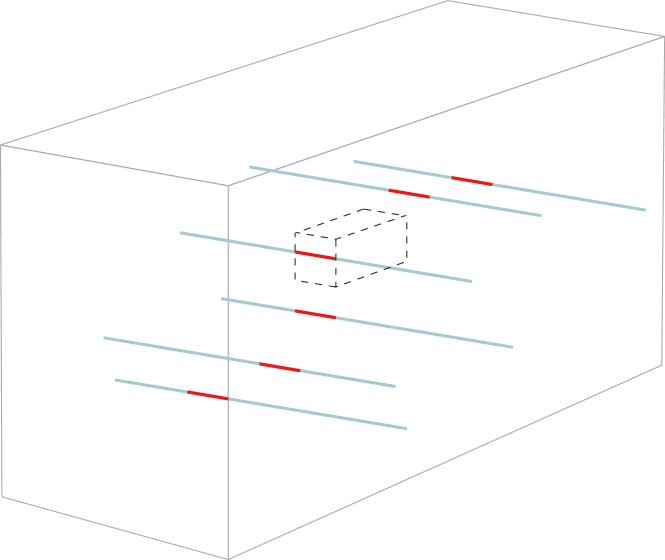
CUR decompositions for matrices have been actively studied [24, 25]. For a matrix , let be a column submatrix of with column indices , be a row submatrix of with row indices , and . The theory of CUR decompositions states that if . The first extension of CUR decompositions to tensors involved a single-mode unfolding of 3-mode tensors [26]. Later, [27] proposes a different variant of tensor CUR that accounts for all modes. Recently, [22] dubs these decompositions with more descriptive monikers, namely Fiber and Chidori CUR decompositions. Later in this paper, we will employ the tensor Fiber CUR decomposition (see Figure 1 for illustration) to accelerate a key step in the proposed algorithm. For the reader’s convenience, we state the characterization of the Fiber CUR decomposition below.
Theorem 2.5 ([22, Theorem 3.3]).
Let with multilinear rank . Let and . Set , and . Then the following statements are equivalent:
-
(i)
,
-
(ii)
,
-
(iii)
for all and the multilinear rank of is .
In particular, (ii) is called tensor Fiber CUR decomposition.
In addition, according to [28, Corollary 5.2], if one uniformly samples indices and with size and , then holds for all with high probability under some mild assumptions. Thus, the tensor Fiber CUR decomposition holds and its computational complexity is dominated by computing the pseudoinverse of . Given the dimension of , computing the pseudoinverse costs flops, thus tensor Fiber CUR decomposition costs flops. In contrast, HOSVD costs flops.
3 Proposed Approach
In this section, we propose a fast approach, called Robust Tensor CUR (RTCUR), for non-convex TRPCA problem (3). RTCUR is developed in a framework of alternating projections: (I) First, we project onto the space of sparse tensors to update the estimate of outliers (i.e., ); (II) then we project the less corrupted data onto the space of low-multilinear-rank tensors to update the estimate (i.e., ). The key for our algorithm acceleration is using tensor Fiber CUR decomposition for inexact low-multilinear-rank tensor approximation in Step (II), which provides much better computational complexity than the standard HOSVD. Consequently, in Step (I), this inexact approximation allows us to estimate only the outliers that lie in the smaller subtensors and fibers that Fiber CUR decomposition samples. RTCUR is summarized in Algorithm 1. Now, we will discuss the details of our approach and start with Step (II).
3.1 Updating
SVD is the most standard method for low-rank approximation in the matrix setting. Similarly, in the literature, HOSVD is the standard method for low-multilinear-rank approximation under our multilinear rank setting. However, HOSVD is computationally expansive when the problem scale is large. Inspired by the recent development on tensor CUR decomposition [22], we employ Fiber CUR decomposition for accelerated inexact low-multilinear-rank tensor approximations and update the estimate by setting
| (8) |
where
| (9) |
for all . Therein, denotes the truncated rank- matrix singular value decomposition that is used to enforce the low-multilinear-rank constraint. Recall the aforementioned complexity for computing Fiber CUR decomposition is . Note that there is no need to compute the full but merely the sampled subtensors. Similarly, forming the entire is never needed through RTCUR—we only need to keep the decomposed tensor components and form the sampled subtensors of accordingly (see Section 3.3 for details). That is, (8) is provided for explanation but should never be fully computed in an efficient implementation of RTCUR.
3.2 Updating
We consider the simple yet effective hard thresholding operator for outlier estimation, which is defined as:
| (10) |
As shown in [4, 5, 2], with a properly chosen thresholding value, is effectively a projection operator onto the support of . More specifically, we update
| (11) |
If is chosen, then we have and . Empirically, we find that iteratively decaying thresholding values
| (12) |
provide superb performance with carefully tuned and . Note that a favorable choice of is , which can be easily accessed/estimated in many applications. The decay factor should be tuned according to the difficulty of the TRPCA problem, e.g., those problems with higher rank, more dense outliers, or large condition number are harder. For successful reconstruction, the harder problems require larger and vice versa. We observe that generally performs well.
3.3 Computational Complexity
As mentioned, the complexity for computing a Fiber CUR decomposition is very low, thus the dominating steps in RTCUR are the hard thresholding operator and/or the tensor/matrix multiplications. We again remark that only the sampled subtensors and fibers are needed when computing (9). Thus, we merely need to estimate the outliers on these subtensors and fibers, and (11) should not be fully executed. Instead, we only compute
| (13) |
for all , which leads to a total complexity of in this step. Not only can we save the computational complexity on hard thresholding but also much smaller subtensors of need to be formed in (13). We can form the required subtensors from the stored Fiber CUR components, which is much cheaper than forming and saving the whole . In particular, the total complexity for forming and is and it dominates the overall complexity of RTCUR.
Moreover, for time saving purposes, we may avoid computing the Frobenius norm of the full tensor when computing the relative error for the stopping criterion. In RTCUR, we adjust the relative error formula to be
| (14) |
where , so that it does not use any extra subtensor or fiber but only those we already formed.
3.4 Two Variants of RTCUR
We consider two variants of RTCUR, namely RTCUR-F and RTCUR-R. RTCUR-F uses fixed sample indices through all iterations while RTCUR-R resamples and in every iteration. RTCUR-F requires minimal data accessibility and runs slightly faster. RTCUR-R accesses more data and takes some extra computing; for example, the denominator of (14) has to be recomputed per iteration. On the other hand, accessing more redundant data means RTCUR-R has a better chance to correct any “unlucky” sampling over the iterations, thus we expect that RTCUR-R has superior outlier tolerance than RTCUR-F. We recommend RTCUR-F if the data accessibility or computation ability is limited. Otherwise, if better outlier tolerance is desired and data is easily accessible, then RTCUR-R is recommended.
4 Numerical Experiments
In this section, we conduct numerical experiments to verify the empirical performance of RTCUR against the state-of-the-art robust matrix/tensor PCA algorithms: Alternating Direction Method of Multipliers for TRPCA (ADMM) [17], Accelerated Alternating Projections for RPCA (AAP) [4], and Iterative Robust CUR for RPCA (IRCUR) [5]. Both proposed variants, RTCUR-F and RTCUR-R, will be evaluated. Section 4.1 contains two synthetic experiments: (i) We study the empirical relation between the outlier tolerance and sample size for RTCUR. (ii) We show the speed advantage of RTCUR compared to the state-of-the-art methods. In Sections 4.2, we successfully apply RTCUR to two real-world problems, color video background subtraction and face modeling.
We utilize the codes of all compared algorithms from the authors’ websites, and the parameters are hand tuned for their best performance. For RTCUR, we sample and for all , and is called the sampling constant through this section. All the tests are executed from Matlab R2020a on an Ubuntu workstation with Intel i9-9940X CPU and 128GB RAM.
| video | runtime (sec) | |||||
|---|---|---|---|---|---|---|
| size | RTCUR-F | RTCUR-R | ADMM [17] | AAP [4] | IRCUR [5] | |
| Shoppingmall | 3.53 | 5.83 | 783.67 | 50.38 | 15.71 | |
| Highway | 3.15 | 5.47 | 168.55 | 18.10 | 3.87 | |
| Crossroad | 6.15 | 13.33 | 1099.3 | 97.85 | 35.47 | |
| Port | 7.22 | 8.10 | 3502.8 | 121.2 | 11.98 | |
| Parking lot | 6.30 | 8.91 | 1001.5 | 43.12 | 9.02 | |
4.1 Synthetic Examples
For the synthetic experiments, we use and . The observed tensor . To generate -mode with multilinear rank , we take where and are Gaussian random tensor and matrices with standard normal entries. To generate the sparse outlier tensor , we uniformly sample percent entries to be the support of and the values of the non-zero entries are uniformly sampled from the interval .
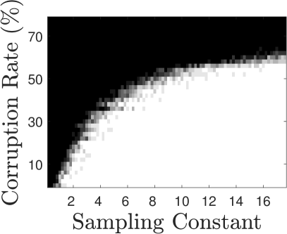
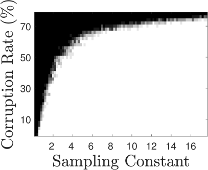
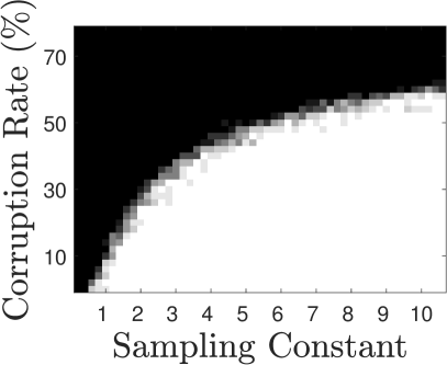
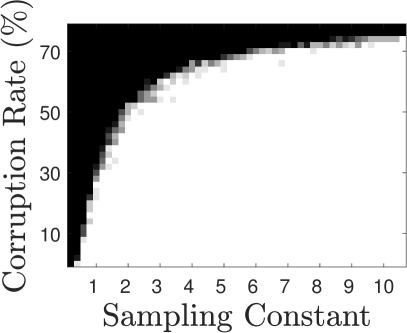
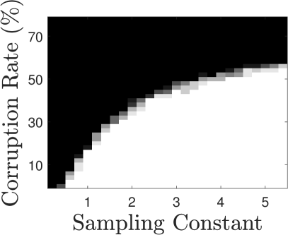
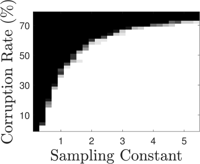
Phase transition. We study the empirical relation between the outlier corruption rate and sampling constant for RTCUR-F and RTCUR-R. The tests are conducted on (i.e., and ) problems with or . For both the variants, the thresholding parameters are set to be and . The stopping condition is and an example is considered successfully solved if . For each pair of and , we generate test examples.
The experimental results are summarized in Figure 2, where a white pixel means all test examples are successfully solved under the corresponding problem parameter setting and a black pixel means all test cases fail. As expected, one can see RTCUR-R has slightly better performance than RTCUR-F and smaller tolerates more outliers since a larger leads to a harder problem. Moreover, taking larger clearly provides better outlier tolerance. However, larger means RTCUR needs to sample larger subtensors and more fibers, which of course leads to more computational time. According to this experiment, we recommend to balance between outlier tolerance and speed.
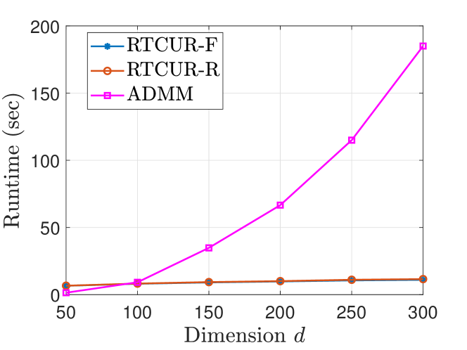
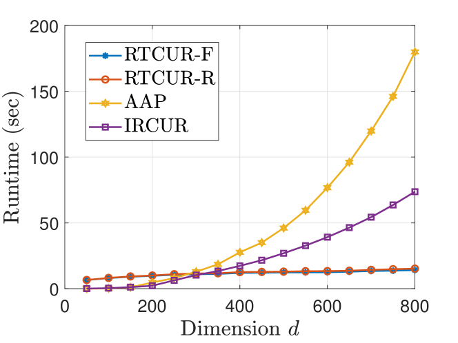
Computational efficiency. In this section, we compare the computational efficiency between RTCUR and the state-of-the-art tensor/matrix RPCA algorithms. For matrix methods, we first unfold a -mode tensor to a matrix, then solve the matrix RPCA problem with rank . For all tests, we add corruption and set parameters , , for both RTCUR-F and RTCUR-R. The reported runtime is averaged over trials.
In Figure 3, we consider the problem of -mode TRPCA with varying dimension and compare the total runtime (all methods halt when ). One can see both variants of RTCUR are substantially faster than the compared algorithms when is large.
4.2 Color Video Background Subtraction
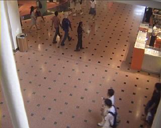
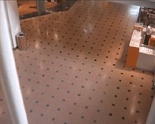
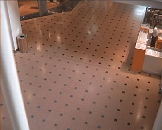
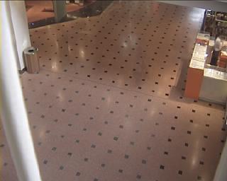
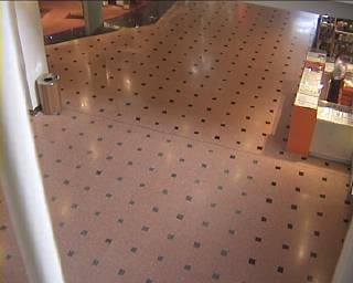
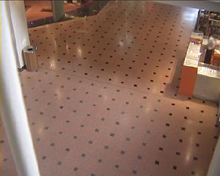
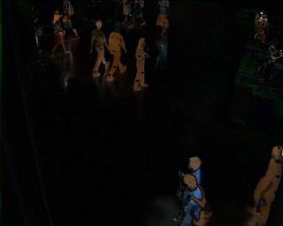
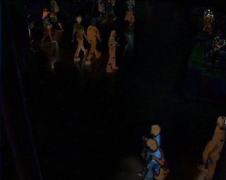
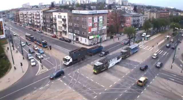
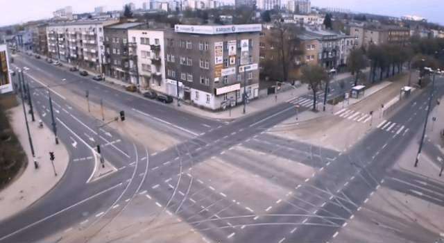
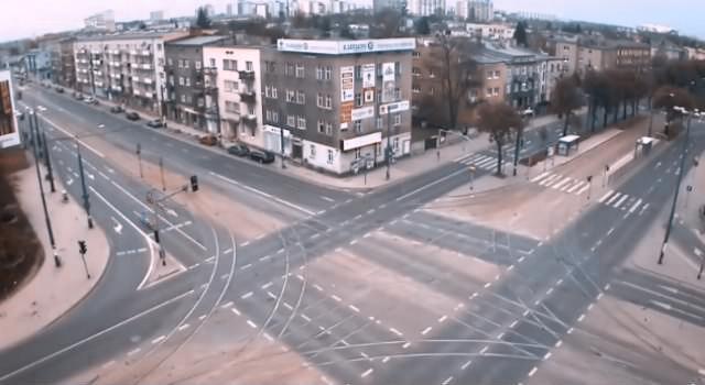
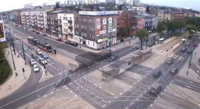
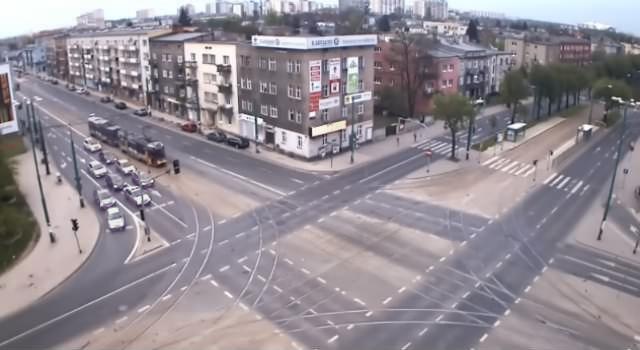
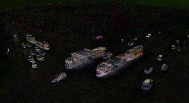
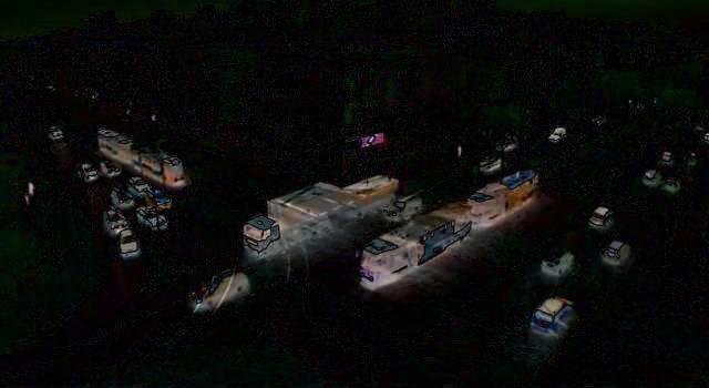
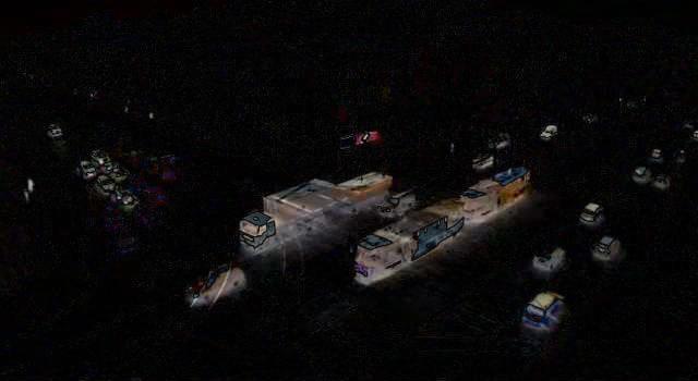
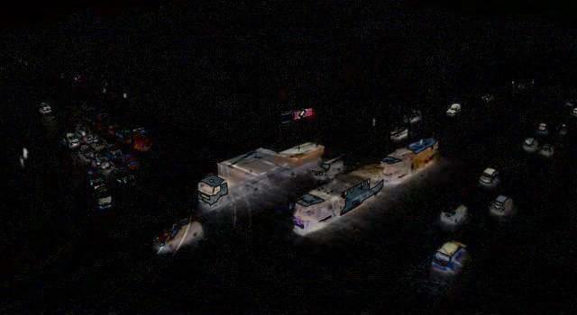
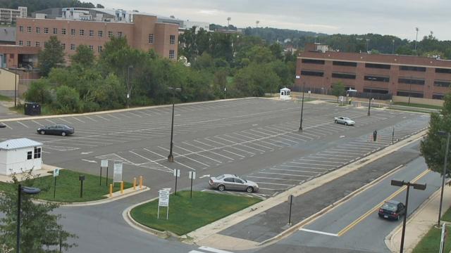
We apply RTCUR on the task of color video background subtraction. We consider two color video datasets with static backgrounds: Shoppingmall [29], Highway [30], Crossroad [30], Port [30], and Parking Lot [31]. Since a monochromatic frame usually does not have low rank structure [32], we vectorize each color channel of each frame into a vector and construct a (height width) frames) tensor. The targeted multilinear rank is for both videos. For those matrix algorithms, we unfold the tensor to a (height width)( frames) matrix and rank is used. We set RTCUR parameters , , in this experiment.
5 Conclusion and Future Work
This paper presents a highly efficient algorithm RTCUR for large-scale TRPCA problems. RTCUR is developed by introducing a novel inexact low-multilinear-rank tensor approximation via Fiber CUR decomposition, whose structure provides a significantly reduced computational complexity. Specifically speaking, RTCUR has per iteration computational complexity as low as flops. Numerical experiments show that RTCUR is superior to other state-of-the-art tensor/matrix RPCA algorithms, on both synthetic and real-world datasets.
There are four lines of future research work. First, it will be important to investigate a theoretical convergence guarantee of RTCUR. Second, extending RTCUR to the partially observed setting (i.e., when only a small random portion of the tensor is observed) is another future direction. Third, we will study the stability of RTCUR with additive dense noise since outliers often present with small dense noise in real-world applications. Last, there are exist tensor PCA studies focusing on the online tensor analysis in order to alleviate the heavy memory cost [33, 34, 35], we will leave this topic to be our future work.










References
- [1] E. J. Candès, X. Li, Y. Ma, and J. Wright, “Robust principal component analysis?,” Journal of the ACM (JACM), vol. 58, no. 3, pp. 1–37, 2011.
- [2] P. Netrapalli, N. U N, S. Sanghavi, A. Anandkumar, and P. Jain, “Non-convex robust PCA,” in Advances in Neural Information Processing Systems (Z. Ghahramani, M. Welling, C. Cortes, N. Lawrence, and K. Q. Weinberger, eds.), vol. 27, Curran Associates, Inc., 2014.
- [3] T. Bouwmans, S. Javed, H. Zhang, Z. Lin, and R. Otazo, “On the applications of robust PCA in image and video processing,” Proceedings of the IEEE, vol. 106, no. 8, pp. 1427–1457, 2018.
- [4] H. Cai, J.-F. Cai, and K. Wei, “Accelerated alternating projections for robust principal component analysis,” The Journal of Machine Learning Research, vol. 20, no. 1, pp. 685–717, 2019.
- [5] H. Cai, K. Hamm, L. Huang, J. Li, and T. Wang, “Rapid robust principal component analysis: CUR accelerated inexact low rank estimation,” IEEE Signal Processing Letters, vol. 28, pp. 116–120, 2020.
- [6] H. Cai, K. Hamm, L. Huang, and D. Needell, “Robust CUR decomposition: Theory and imaging applications,” arXiv preprint arXiv:2101.05231, 2021.
- [7] J. Wright, A. Y. Yang, A. Ganesh, S. S. Sastry, and Y. Ma, “Robust face recognition via sparse representation,” IEEE transactions on pattern analysis and machine intelligence, vol. 31, no. 2, pp. 210–227, 2008.
- [8] Y. Hu, J.-X. Liu, Y.-L. Gao, and J. Shang, “DSTPCA: Double-sparse constrained tensor principal component analysis method for feature selection,” IEEE/ACM Transactions on Computational Biology and Bioinformatics, 2019.
- [9] H. Cai, J.-F. Cai, T. Wang, and G. Yin, “Accelerated structured alternating projections for robust spectrally sparse signal recovery,” IEEE Transactions on Signal Processing, vol. 69, pp. 809–821, 2021.
- [10] L. Li, W. Huang, I. Y.-H. Gu, and Q. Tian, “Statistical modeling of complex backgrounds for foreground object detection,” IEEE Transactions on Image Processing, vol. 13, no. 11, pp. 1459–1472, 2004.
- [11] B. Huang, C. Mu, D. Goldfarb, and J. Wright, “Provable low-rank tensor recovery,” Optimization-Online, vol. 4252, no. 2, pp. 455–500, 2014.
- [12] Q. Gu, H. Gui, and J. Han, “Robust tensor decomposition with gross corruption,” Advances in Neural Information Processing Systems, vol. 27, pp. 1422–1430, 2014.
- [13] S. E. Sofuoglu and S. Aviyente, “A two-stage approach to robust tensor decomposition,” in 2018 IEEE Statistical Signal Processing Workshop (SSP), pp. 831–835, IEEE, 2018.
- [14] Y. Hu and D. B. Work, “Robust tensor recovery with fiber outliers for traffic events,” ACM Transactions on Knowledge Discovery from Data (TKDD), vol. 15, no. 1, pp. 1–27, 2020.
- [15] Z. Zhang, G. Ely, S. Aeron, N. Hao, and M. Kilmer, “Novel methods for multilinear data completion and de-noising based on tensor-SVD,” in Proceedings of the IEEE conference on computer vision and pattern recognition, pp. 3842–3849, 2014.
- [16] Y. Liu, L. Chen, and C. Zhu, “Improved robust tensor principal component analysis via low-rank core matrix,” IEEE Journal of Selected Topics in Signal Processing, vol. 12, no. 6, pp. 1378–1389, 2018.
- [17] C. Lu, J. Feng, Y. Chen, W. Liu, Z. Lin, and S. Yan, “Tensor robust principal component analysis with a new tensor nuclear norm,” IEEE transactions on pattern analysis and machine intelligence, vol. 42, no. 4, pp. 925–938, 2019.
- [18] F. L. Hitchcock, “The expression of a tensor or a polyadic as a sum of products,” Journal of Mathematical Physics, vol. 6, no. 1-4, pp. 164–189, 1927.
- [19] A. Anandkumar, P. Jain, Y. Shi, and U. N. Niranjan, “Tensor vs. matrix methods: Robust tensor decomposition under block sparse perturbations,” in Artificial Intelligence and Statistics, pp. 268–276, PMLR, 2016.
- [20] F. L. Hitchcock, “Multiple invariants and generalized rank of a -way matrix or tensor,” Journal of Mathematical Physics, vol. 7, no. 1-4, pp. 39–79, 1928.
- [21] D. Goldfarb and Z. Qin, “Robust low-rank tensor recovery: Models and algorithms,” SIAM Journal on Matrix Analysis and Applications, vol. 35, no. 1, pp. 225–253, 2014.
- [22] H. Cai, K. Hamm, L. Huang, and D. Needell, “Mode-wise tensor decompositions: Multi-dimensional generalizations of CUR decompositions,” The Journal of Machine Learning Research, vol. 22, no. 185, pp. 1–36, 2021.
- [23] L. De Lathauwer, B. De Moor, and J. Vandewalle, “On the best rank-1 and rank-() approximation of higher-order tensors,” SIAM Journal on Matrix Analysis and Applications, vol. 21, no. 4, pp. 1324–1342, 2000.
- [24] S. A. Goreĭnov, N. L. Zamarashkin, and E. E. Tyrtyshnikov, “Pseudo-skeleton approximations,” Doklay Akdemii Nauk, vol. 343, no. 2, pp. 151–152, 1995.
- [25] K. Hamm and L. Huang, “Perspectives on CUR decompositions,” Applied and Computational Harmonic Analysis, vol. 48, no. 3, pp. 1088–1099, 2020.
- [26] M. W. Mahoney, M. Maggioni, and P. Drineas, “Tensor-CUR decompositions for tensor-based data,” SIAM Journal on Matrix Analysis and Applications, vol. 30, no. 3, pp. 957–987, 2008.
- [27] C. F. Caiafa and A. Cichocki, “Generalizing the column–row matrix decomposition to multi-way arrays,” Linear Algebra and its Applications, vol. 433, no. 3, pp. 557–573, 2010.
- [28] K. Hamm and L. Huang, “Stability of sampling for CUR decompositions,” Foundations of Data Science, vol. 2, no. 2, p. 83, 2020.
- [29] E. L, “Foreground detection in video sequences with probabilistic self-organizing maps.”
- [30] T. Bouwmans, L. Maddalena, and A. Petrosino, “Scene background initialization: A taxonomy,” Pattern Recognition Letters, vol. 96, pp. 3–11, 2017.
- [31] S. Oh, A. Hoogs, A. Perera, N. Cuntoor, C.-C. Chen, J. T. Lee, S. Mukherjee, J. Aggarwal, H. Lee, L. Davis, et al., “A large-scale benchmark dataset for event recognition in surveillance video,” in CVPR 2011, pp. 3153–3160, IEEE, 2011.
- [32] Z. Chao, L. Huang, and D. Needell, “Tensor completion through total variation with initialization from weighted hosvd,” in 2020 Information Theory and Applications Workshop (ITA), pp. 1–8, IEEE, 2020.
- [33] A. Sobral, C. G. Baker, T. Bouwmans, and E.-h. Zahzah, “Incremental and multi-feature tensor subspace learning applied for background modeling and subtraction,” in International Conference Image Analysis and Recognition, pp. 94–103, Springer, 2014.
- [34] P. Li, J. Feng, X. Jin, L. Zhang, X. Xu, and S. Yan, “Online robust low-rank tensor modeling for streaming data analysis,” IEEE transactions on neural networks and learning systems, vol. 30, no. 4, pp. 1061–1075, 2018.
- [35] J. Bin, M. Kang, and Z. Liu, “Gpu-accelerated tensor decomposition for moving object detection from multimodal imaging,” in 2020 IEEE Sensors, pp. 1–4, IEEE, 2020.