Resource Allocation in Heterogeneously-Distributed
Joint Radar-Communications under
Asynchronous Bayesian Tracking Framework

Linlong Wu,  Kumar Vijay Mishra,  Bhavani Shankar M. R.,  and Björn Ottersten The authors are with the Interdisciplinary Centre for Security, Reliability and Trust (SnT), University of Luxembourg, Luxembourg City L-1855, Luxembourg. E-mail: {linlong.wu@, kumar.mishra@ext., bhavani.shankar@, bjorn.ottersten@}uni.lu. Corresponding author: Linlong Wu.Their work is supported in part by ERC AGNOSTIC under grant EC/H2020/ERC2016ADG/742648 and in part by FNR CORE SPRINGER under grant C18/IS/12734677.The conference precursor of this work was presented in the 2021 IEEE International Workshop on Signal Processing Advances in Wireless Communications (SPAWC).
Abstract

Optimal allocation of shared resources is key to deliver the promise of jointly operating radar and communications systems. In this paper, unlike prior works which examine synergistic access to resources in colocated joint radar-communications or among identical systems, we investigate this problem for a distributed system comprising heterogeneous radars and multi-tier communications. In particular, we focus on resource allocation in the context of multi-target tracking (MTT) while maintaining stable communications connections. By simultaneously allocating the available power, dwell time and shared bandwidth, we improve the MTT performance under a Bayesian tracking framework and guarantee the communications throughput. Our alternating allocation of heterogeneous resources (ANCHOR) approach solves the resulting non-convex problem based on the alternating optimization method that monotonically improves the Bayesian Cramér-Rao bound. Numerical experiments demonstrate that ANCHOR significantly improves the tracking error over two baseline allocations and stability under different target scenarios and radar-communications network distributions.

Index Terms:
Bayesian Cramér-Rao bound, heterogeneous radar networks, joint radar-communications, multi-target tracking, resource allocation.

I Introduction

Spectrum sharing between radar and communications systems has lately garnered significant research interest in order to efficiently exploit the electromagnetic spectrum, a scarce natural resource [1, 2]. While radars require wider bandwidths to deliver a high-resolution sensing performance [3], mobile communications are witnessing an ever-increasing demand for broader bandwidths in order to provide a designated quality-of-service (QoS) [4]. Spectrum-sharing solutions address these competing requirements either by opportunistic spectral access of broadcast systems by passive radars [5]; spectrally coexisting legacy systems that operate by mitigating the mutual interference with minimum design modifications at the cost of performance [6, 7, 8]; or spectrally co-designed joint radar-communications (JRC) systems [9, 10, 11] that utilize a common transmit/receive hardware and waveform.

A successful operation of these spectrum sharing systems relies on an efficient radio resource optimization [12, 13, 14]. In coexistence paradigms with single antenna or with a fixed beamforming, the resources may include total transmit power, transmit signal bandwidth, and transmission time slots [9]. Additionally, in phased array or multiple-input multiple-output (MIMO) systems, antennas need to be reserved for optimal sharing [15]. In single antenna JRC systems, the resource allocation objective is to optimize the transmit energy of the dual-purpose waveform based on the propagation channels of radar and communications users. In JRC systems employing a transmit antenna array, highly directional beamforming toward the radar surveillance area while also ensuring sidelobes on the users offers an interesting solution [16]. In JRC systems involving hybrid analog-digital transceiver architectures [17], antenna selection may also be viewed as a component of resource allocation objective.

While colocated JRC solutions continue to be comprehensively investigated, distributed JRC systems involving widely separated radars and communications transmitters remain relatively unexamined. Among prior works, the spectrum-sharing model in [18] comprises a widely distributed MIMO radar [19] but studies coexistence with a simplistic point-to-point MIMO communications. The distributed radar proposed in [20] exploits a communications waveform but operates in passive (receive-only) mode. The co-design framework in [21] develops new waveforms and precoders for a distributed but identical units of radar and communications. The displaced sensor imaging in [22] considers identical units of radar sensors on the same vehicular platform that coordinate timing via communications protocols.

There are very few resource allocation studies for identical or homogeneous distributed JRC systems [23]. In such a system, the objective is to optimize the transmission strategies (e.g., transmit power, duration, bandwidth) for identical transmit systems in order to minimize the target localization error in a dynamic scenario and maximize the communications capacity. In the context of distributed radar resource allocation for target localization and tracking, seminal works have appeared recently [24, 25, 26, 27, 28]. In [24], a joint beam and power allocation scheme was developed for a colocated MIMO radar network. In [25], target assignment and dwell time allocation were considered simultaneously in a phased array radar network. Subsequently, in [26], an adaptive power allocation was proposed with dynamic tracking threshold adjustment based on the asynchronous working manner of the radar networks. This was extended in [27] by considering heterogeneous radar (HetRad) network, i.e. comprising different types of radar units, for multi-target tracking (MTT).

However, aforementioned prior works do not consider spectrum sharing paradigm with wireless communications. Additionally, the distributed nature of radar deployment, strong likelihood of encountering heterogeneous radar units in practice, and an ever-increasing deployment of cellular communications potentially makes optimal resource allocation difficult in a dynamic scenario. In each of these cases, the resulting spectrum reuse leads to interference between the two systems and impacts the resource allocation strategy. In [23], resource allocation is considered for target localization excluding additional complexities of a heterogeneous radar network and multi-tier communications. Some recent state-of-the-art works [29, 30] on combining sensing functionalities in heterogeneous wireless networks (HetNets) explore the effect of varied communications coverage areas on the joint system performance. However, these studies do not explore resource allocation and do not, per se, qualify as JRC systems.

In this paper, we consider a heterogeneous mix of radar units and multi-tier communications to propose optimal allocation of resources such as power, dwell time, and bandwidth. Our approach optimizes the radar tracking performance while maintaining a reliable QoS in communications systems. Preliminary results of this work appeared in our conference publication [31] where multi-tier communications and various systems configurations were ignored. In this work, we further generalize the study in [31] to the following aspects: First, from system model perspective, we include target Doppler in the radar measurement model and estimate all key parameters, - range, angle-of-arrival (AOA), and Doppler velocity - of a target. Next, we model the communications system as a multi-tier cellular network. We also consider the allocation of the shared frequency bands besides power and dwell time in the joint HetRad-HetNet scenario. Finally, a novel algorithm based on the alternating optimization framework is developed to solve the resulting non-convex problem. For each subproblem, we further propose an iterative method to solve with low computational complexity and proven convergence analyses. Our proposed alternating allocation of heterogeneous resources (ANCHOR) algorithm for distributed resource allocation shows roughly 101010 times improvement of tracking performance in the sense of root mean square error over the baseline allocations.

The rest of this paper is organized as follows. In the next section, we introduce the configurations and system model of the heterogeneous JRC network. We formulate the resource allocation problem in Section III and describe the proposed ANCHOR algorithm in Section IV. We validate our models and methods via numerical experiments in Section V. We conclude in Section VI.

Throughout the paper, we reserve boldface lowercase and boldface uppercase for vectors and matrices, respectively. We denote the transpose, conjugate, and Hermitian by ()Tsuperscript𝑇(\cdot)^{T}, ()superscript(\cdot)^{*}, and ()Hsuperscript𝐻(\cdot)^{H}, respectively. The notation 𝐈Nsubscript𝐈𝑁\mathbf{I}_{N} is the N×N𝑁𝑁N\times N identity matrix, and 𝟏Nsubscript1𝑁\boldsymbol{1}_{N} is a vector with all N𝑁N elements being 1. The Kronecker product is denoted by tensor-product\otimes; ||||p||\cdot||_{p} is the psubscript𝑝\ell_{p} norm; and 0\left\|\cdot\right\|_{0} is the number of non-zero elements of the vector. The notation Tr{}Tr\text{Tr}\left\{\cdot\right\} is the trace of the matrix, |||\cdot| is the cardinality of a set, 𝔼[]𝔼delimited-[]\mathbb{E}\left[\cdot\right] is the statistical expectation function, \nabla is the gradient operator, and 𝒩(,)𝒩\mathcal{N}\left(\cdot,\cdot\right) represents the probability density function of the normal distribution. Table I summarizes some of the important notations in this paper.

TABLE I: Glossary of notations
Symbol Description
N𝑁N Total number of radars
Ncsubscript𝑁𝑐N_{c} Number of colocated MIMO radars
Npsubscript𝑁𝑝N_{p} Number of phased array radars
Nmsubscript𝑁𝑚N_{m} Number of mechanical scanning radars
φcsubscript𝜑𝑐\varphi_{c} Index set of colocated MIMO radars
φpsubscript𝜑𝑝\varphi_{p} Index set of phased array radars
φmsubscript𝜑𝑚\varphi_{m} Index set of mechanical scanning radars
(xi,yi)subscript𝑥𝑖subscript𝑦𝑖\left(x_{i},y_{i}\right) Coordinates of radar i𝑖i
Mi,q,ksubscript𝑀𝑖𝑞𝑘M_{i,q,k} number of measurements on target q𝑞q by radar i𝑖i in fusion interval k𝑘k
ti,q,kmsuperscriptsubscript𝑡𝑖𝑞𝑘𝑚t_{i,q,k}^{m} arrival time of the m𝑚m-th measurement
Pi,q,kmsuperscriptsubscript𝑃𝑖𝑞𝑘𝑚P_{i,q,k}^{m} Power corresponding to receiving time ti,q,kmsuperscriptsubscript𝑡𝑖𝑞𝑘𝑚t_{i,q,k}^{m}
Ti,q,kmsuperscriptsubscript𝑇𝑖𝑞𝑘𝑚T_{i,q,k}^{m} Dwell time corresponding to receiving time ti,q,kmsuperscriptsubscript𝑡𝑖𝑞𝑘𝑚t_{i,q,k}^{m}
T0subscript𝑇0T_{0} Period of fusion interval
J𝐽J Number of communications macro users
L𝐿L Number of communications micro users
βjsuperscript𝛽𝑗\beta^{j} Transmission channel gain
αj,irsuperscriptsubscript𝛼𝑗𝑖𝑟\alpha_{j,i}^{r} Interference channel gain from radar i𝑖i to user j𝑗j
αi,jcsuperscriptsubscript𝛼𝑖𝑗𝑐\alpha_{i,j}^{c} Interference channel gain from userv j𝑗j to radar i𝑖i
σc,j2superscriptsubscript𝜎𝑐𝑗2\sigma_{c,j}^{2} Communications noise power
δjsuperscript𝛿𝑗\delta^{j} Interference channel gain from macro user j𝑗j
Pcjsuperscriptsubscript𝑃𝑐𝑗P_{c}^{j} Power from user j𝑗j
ΔfΔ𝑓\Delta f subchannel bandwidth
B𝐵B Total available bandwidth
F𝐹F Number of subchannels
Fcjsuperscriptsubscript𝐹𝑐𝑗F_{c}^{j} Number of subchannels for user j𝑗j
Frisuperscriptsubscript𝐹𝑟𝑖F_{r}^{i} Number of subchannels for radar i𝑖i
Fi,josuperscriptsubscript𝐹𝑖𝑗𝑜F_{i,j}^{o} Number of overlapped subchannels between radar i𝑖i and user j𝑗j
𝒇j,kcsuperscriptsubscript𝒇𝑗𝑘𝑐\boldsymbol{f}_{j,k}^{c} Subchannel selection vector of user j𝑗j
𝒇i,krsuperscriptsubscript𝒇𝑖𝑘𝑟\boldsymbol{f}_{i,k}^{r} Subchannel selection vector of radar i𝑖i
α~i,jcsuperscriptsubscript~𝛼𝑖𝑗𝑐\tilde{\alpha}_{i,j}^{c} Fourier coefficients ym,qpsuperscriptsubscript𝑦𝑚𝑞𝑝y_{m,q}^{p} after focusing at frequency ν𝜈\nu
N𝑁N Number of Fourier coefficients in each channel
α~j,irsuperscriptsubscript~𝛼𝑗𝑖𝑟\tilde{\alpha}_{j,i}^{r} Set of sampled Fourier coefficients per channel
𝒔i,q,kmsuperscriptsubscript𝒔𝑖𝑞𝑘𝑚\boldsymbol{s}_{i,q,k}^{m} State of target q𝑞q from radar i𝑖i at ti,q,kmsuperscriptsubscript𝑡𝑖𝑞𝑘𝑚t_{i,q,k}^{m}
𝒚i,q,kmsuperscriptsubscript𝒚𝑖𝑞𝑘𝑚\boldsymbol{y}_{i,q,k}^{m} Measurement of target q𝑞q from radar i𝑖i at ti,q,kmsuperscriptsubscript𝑡𝑖𝑞𝑘𝑚t_{i,q,k}^{m}
xi,q,km(yi,q,km)superscriptsubscript𝑥𝑖𝑞𝑘𝑚superscriptsubscript𝑦𝑖𝑞𝑘𝑚x_{i,q,k}^{m}(y_{i,q,k}^{m}) Coordinate x (y) of target q𝑞q at time ti,q,kmsuperscriptsubscript𝑡𝑖𝑞𝑘𝑚t_{i,q,k}^{m}
x˙i,q,km(y˙i,q,km)superscriptsubscript˙𝑥𝑖𝑞𝑘𝑚superscriptsubscript˙𝑦𝑖𝑞𝑘𝑚\dot{x}_{i,q,k}^{m}(\dot{y}_{i,q,k}^{m}) Velocity along x (y) axis of target q𝑞q at time ti,q,kmsuperscriptsubscript𝑡𝑖𝑞𝑘𝑚t_{i,q,k}^{m}

II Network Configuration and System Model

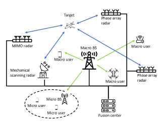
Consider a heterogeneously-distributed radar and communications network (HRCN) (Figure 1), which employs different types of radars that simultaneously track multiple targets. The radars operate in the same spectrum as a multi-tier communications system that comprises a macro base station (BS) and multiple micro and macro users. The HRCN is equipped with a fusion center for signalling, synchronization, and resource allocation. Here, an efficient use of spectrum is possible provided the resources are well allocated amongst radar and communications entities. The HRCN is embedded with the following heterogeneities:

Heterogeneity in network architecture

The HRCN has both radar and cellular network components. The radar network comprises MIMO, phased array, and mechanically scanning radars that are heterogeneously distributed while tracking the same target. The multi-tier cellular communications network has macro and micro BSs along with multiple macro users.

Heterogeneity in allocated resources

Both tracking and communications QoS are affected by respective signal-to-interference-plus-noise ratios (SINRs), which further depend on the transmit power, radar’s dwell time, and bandwidth usage. To mitigate the mutual interference and enhance the overall performance, these heterogeneous resources must be judiciously allocated.

In the following, we describe each of these HRCN configurations in detail.
Refer to caption
Figure 1: An illustration of HRCN, wherein radar and cellular networks share the spectrum and their signals are source of mutual interference.

II-A Configurations of the HRCN

The HRCN is a complex system with several operating units of radars and communications that require numerous system parameters to be optimized for multiple resources.

Radar set-up

Consider N𝑁N radars in the HRCN to track Q𝑄Q widely separated point-like targets in the surrounding environment. In particular, assume Ncsubscript𝑁𝑐N_{c} colocated MIMO radars, Npsubscript𝑁𝑝N_{p} phased array radars, and Nmsubscript𝑁𝑚N_{m} mechanical scanning radars with N=Nc+Np+Nm𝑁subscript𝑁𝑐subscript𝑁𝑝subscript𝑁𝑚N=N_{c}+N_{p}+N_{m}, located at different places with the coordinates {(xi,yi)}i=1Nsuperscriptsubscriptsubscript𝑥𝑖subscript𝑦𝑖𝑖1𝑁\left\{\left(x_{i},y_{i}\right)\right\}_{i=1}^{N}. Define the sets φc{1,,Nc}subscript𝜑𝑐1subscript𝑁𝑐\varphi_{c}\triangleq\left\{1,\ldots,N_{c}\right\}, φp{Nc+1,,Nc+Np}subscript𝜑𝑝subscript𝑁𝑐1subscript𝑁𝑐subscript𝑁𝑝\varphi_{p}\triangleq\left\{N_{c}+1,\ldots,N_{c}+N_{p}\right\}, and φm{Nc+Np+1,,N}subscript𝜑𝑚subscript𝑁𝑐subscript𝑁𝑝1𝑁\varphi_{m}\triangleq\left\{N_{c}+N_{p}+1,\ldots,N\right\} to index these radars. The operational scheme of each of the radars are as follows:

Colocated MIMO radar

For iφc𝑖subscript𝜑𝑐i\in\varphi_{c}, the radar i𝑖i is capable of pointing multiple beams to illuminate multiple targets simultaneously. Herein, the multiple targets are illuminated for the same dwell time but with different transmit powers. Hence, the revisit time intervals for the Q𝑄Q targets are the same.

Phased array radar

For iφp𝑖subscript𝜑𝑝i\in\varphi_{p}, the radar i𝑖i steers the beam to illuminate multiple targets sequentially by configuring the phases of the transmit array. In this scheme, each target is illuminated with identical transmit power but with a different dwell time. Hence, the revisit time intervals for the Q𝑄Q targets are usually different.

Mechanical scanning radar

For radars indexed by φmsubscript𝜑𝑚\varphi_{m}, the system parameters are usually fixed. The radar scans mechanically and illuminates all the targets sequentially with identical power and dwell time (and hence identical revisit times).

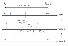
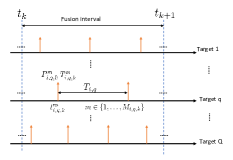
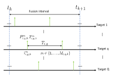
The scanning operations of each radar are depicted in Figure 2, where Mi,q,ksubscript𝑀𝑖𝑞𝑘M_{i,q,k} is the number of measurements collected from target q𝑞q by radar i𝑖i during the k𝑘k-th fusion interval111Fusion interval [32, 33] is the period during which multiple sensors measure and estimate independently. The target state is determined by fusing all radar estimates. (from tksubscript𝑡𝑘t_{k} to tk+1subscript𝑡𝑘1t_{k+1}); ti,q,kmsuperscriptsubscript𝑡𝑖𝑞𝑘𝑚t_{i,q,k}^{m} is the arrival time of the m𝑚m-th measurement for m=1,,Mi,q,k𝑚1subscript𝑀𝑖𝑞𝑘m=1,\ldots,M_{i,q,k}; Pi,q,kmsuperscriptsubscript𝑃𝑖𝑞𝑘𝑚P_{i,q,k}^{m} and Ti,q,kmsuperscriptsubscript𝑇𝑖𝑞𝑘𝑚T_{i,q,k}^{m} denote, respectively, the transmit power and dwell time corresponding to the measurement at time ti,q,kmsuperscriptsubscript𝑡𝑖𝑞𝑘𝑚t_{i,q,k}^{m}. Assume that the fusion interval is a constant denoted by T0subscript𝑇0T_{0}. The inter-measurement duration (Fig. 2a) at i𝑖ith MIMO radar for the q𝑞qth target (revisit intervals) is denoted by a constant Ti,qsubscript𝑇𝑖𝑞T_{i,q}. However, Pi,q,kmsuperscriptsubscript𝑃𝑖𝑞𝑘𝑚P_{i,q,k}^{m} varies for q=1,Q𝑞1𝑄q=1,\ldots Q. In case of phased-array radars (Fig. 2b), Ti,qsubscript𝑇𝑖𝑞T_{i,q} are different but Pi,q,kmsuperscriptsubscript𝑃𝑖𝑞𝑘𝑚P_{i,q,k}^{m} is identical for q=1,Q𝑞1𝑄q=1,\ldots Q. Finally, for a mechanically scanning radar (Fig. 2c), both Ti,qsubscript𝑇𝑖𝑞T_{i,q} and Pi,q,kmsuperscriptsubscript𝑃𝑖𝑞𝑘𝑚P_{i,q,k}^{m} are the same for q=1,Q𝑞1𝑄q=1,\ldots Q.

Refer to caption
(a) Colocated MIMO radar.
Refer to caption
(b) Phased array radar.
Refer to caption
(c) Mechanical scanning radar.
Figure 2: Illustrations of scanning operations for (a) colocated MIMO, (b) phased array, and (c) mechanically scanning radars, where Mi,q,ksubscript𝑀𝑖𝑞𝑘M_{i,q,k} is the number of measurements collected from target q𝑞q by radar i𝑖i during the k𝑘k-th fusion interval (from tksubscript𝑡𝑘t_{k} to tk+1subscript𝑡𝑘1t_{k+1}); ti,q,kmsuperscriptsubscript𝑡𝑖𝑞𝑘𝑚t_{i,q,k}^{m} is the arrival time of the m𝑚m-th measurement for m=1,,Mi,q,k𝑚1subscript𝑀𝑖𝑞𝑘m=1,\ldots,M_{i,q,k}; and Pi,q,kmsuperscriptsubscript𝑃𝑖𝑞𝑘𝑚P_{i,q,k}^{m} and Ti,q,kmsuperscriptsubscript𝑇𝑖𝑞𝑘𝑚T_{i,q,k}^{m} are,, respectively, the transmit power and dwell time corresponding to the measurement at time ti,q,kmsuperscriptsubscript𝑡𝑖𝑞𝑘𝑚t_{i,q,k}^{m}.
Wireless communications configuration

Consider a multi-tier heterogeneous network (HetNet) of communications (Fig. 1) that consists of a macrocell (primary network) with multiple macro users and a microcell (secondary network). The primary network of the macro BS serves J𝐽J macro users and one micro BS. The secondary network is served by the micro BS with L𝐿L micro users. The co-existence of the multi-tier networks, frequency reuse, and precoding has been well-studied in literature [34]. For the HRCN resource allocation, we make the following model to simplify the problem.

Communications downlinks

The coverage areas of the macro and micro BSs are different. When reusing the frequencies, we assume that the macro downlinks cause interfere to only L𝐿L micro users. Similarly, the micro downlinks interfere within the coverage area of only micro BS. This is especially true when the micro network is power limited.

SINR of macro user

The macro BS employs orthogonal frequency-division multiple access (OFDMA) for downlink and allocates non-interfering resource blocks. As a result, the mutual interference among the J𝐽J macro downlinks is non-existent. The SINR of the j𝑗j-th macro user is222The radar illumination is irregular and non-continuous in a fusion interval. Hence, the commonly used transient SINR is unavailable. Instead, we use the average SINR as the communications metric. Additionally, the averaging period may be replaced by the airtime Tcsubscript𝑇𝑐T_{c} of the communications transmission, which has the same expression but with a scaling constant Tc/T0subscript𝑇𝑐subscript𝑇0T_{c}/T_{0}.

SINRj=βjPcjT0i=1Nq=1Qm=1Mi,q,kαj,irPi,q,kmTi,q,km+σc,j2T0,subscriptSINR𝑗superscript𝛽𝑗superscriptsubscript𝑃𝑐𝑗subscript𝑇0superscriptsubscript𝑖1𝑁superscriptsubscript𝑞1𝑄superscriptsubscript𝑚1subscript𝑀𝑖𝑞𝑘superscriptsubscript𝛼𝑗𝑖𝑟superscriptsubscript𝑃𝑖𝑞𝑘𝑚superscriptsubscript𝑇𝑖𝑞𝑘𝑚superscriptsubscript𝜎𝑐𝑗2subscript𝑇0\text{SINR}_{j}=\frac{\beta^{j}P_{c}^{j}T_{0}}{\sum_{i=1}^{N}\sum_{q=1}^{Q}\sum_{m=1}^{M_{i,q,k}}\alpha_{j,i}^{r}P_{i,q,k}^{m}T_{i,q,k}^{m}+\sigma_{c,j}^{2}T_{0}}, (1)

where βjsuperscript𝛽𝑗\beta^{j} and Pcjsuperscriptsubscript𝑃𝑐𝑗P_{c}^{j} are the channel gain and allocated power to the j𝑗j-th macro entity, respectively; αj,irsuperscriptsubscript𝛼𝑗𝑖𝑟\alpha_{j,i}^{r} is the interference channel gain from the i𝑖i-th radar; and σc,j2superscriptsubscript𝜎𝑐𝑗2\sigma_{c,j}^{2} is the noise power at the receiver front-end of j𝑗jth user.

SINR of micro user

To improve spectrum utilization, the micro BS may reuse the same band of the macro BS [35] and then apply the (non-interfering) OFDMA resource blocks amongst the L𝐿L micro users. This leads to negligible mutual interference among the L𝐿L micro users. Compared to the SINR of macro entities, the SINR for the l𝑙l-th micro user becomes

SINRl=βlPclT0δjPcjT0+i=1Nq=1Qm=1Mi,q,kαl,irPi,q,kmTi,q,km+σc,l2T0,subscriptSINR𝑙superscript𝛽𝑙superscriptsubscript𝑃𝑐𝑙subscript𝑇0superscript𝛿𝑗superscriptsubscript𝑃𝑐𝑗subscript𝑇0superscriptsubscript𝑖1𝑁superscriptsubscript𝑞1𝑄superscriptsubscript𝑚1subscript𝑀𝑖𝑞𝑘superscriptsubscript𝛼𝑙𝑖𝑟superscriptsubscript𝑃𝑖𝑞𝑘𝑚superscriptsubscript𝑇𝑖𝑞𝑘𝑚superscriptsubscript𝜎𝑐𝑙2subscript𝑇0\displaystyle\small{\text{SINR}_{l}}=\small{\frac{\beta^{l}P_{c}^{l}T_{0}}{\delta^{j}P_{c}^{j}T_{0}+\sum_{i=1}^{N}\sum_{q=1}^{Q}\sum_{m=1}^{M_{i,q,k}}\alpha_{l,i}^{r}P_{i,q,k}^{m}T_{i,q,k}^{m}+\sigma_{c,l}^{2}T_{0}},} (2)

where δjPcjT0superscript𝛿𝑗superscriptsubscript𝑃𝑐𝑗subscript𝑇0\delta^{j}P_{c}^{j}T_{0} represents the interference from the j𝑗j-th macro user of the same frequency; δjsuperscript𝛿𝑗\delta^{j} is the interference channel gain; and the other parameters are similar to their counterparts in (1).

Codebook

We assume Gaussian codebook for all transmissions.

Configurations for shared bandwidth

Assume B𝐵B to be the total bandwidth available to the HRCN. The sub-carrier interval of OFDMA ΔfΔ𝑓\Delta f and the spectrum is divided into F𝐹F sub-channels with B=Δf(F1)𝐵Δ𝑓𝐹1B=\Delta f\left(F-1\right). The allocated bandwidth is configured as follows:

Bandwidth configuration for communications

To serve the J𝐽J macro entities, the communications network requires Fcsubscript𝐹𝑐F_{c} sub-channels with Fc=j=1JFcjsubscript𝐹𝑐superscriptsubscript𝑗1𝐽superscriptsubscript𝐹𝑐𝑗F_{c}=\sum_{j=1}^{J}F_{c}^{j}, where Fcjsuperscriptsubscript𝐹𝑐𝑗F_{c}^{j} is the number of sub-channels for the j𝑗j-th user. A selection vector 𝒇j,kcFsuperscriptsubscript𝒇𝑗𝑘𝑐superscript𝐹\boldsymbol{f}_{j,k}^{c}\in\mathbb{R}^{F}, comprising of binary entries, represents the selected sub-channels for the j𝑗j-th downlink in the k𝑘k-th fusion interval. Similar operations are ascribed to the L𝐿L micro users. The bandwidth allocation (i.e. {𝒇j,kc}j=1Jsuperscriptsubscriptsuperscriptsubscript𝒇𝑗𝑘𝑐𝑗1𝐽\left\{\boldsymbol{f}_{j,k}^{c}\right\}_{j=1}^{J}) may be reassigned for each fusion interval to meet the changing demands of the wireless communications.

Bandwidth configuration for radars

The bandwidth required by the i𝑖i-th radar is Bi=ΔfFrisubscript𝐵𝑖Δ𝑓superscriptsubscript𝐹𝑟𝑖B_{i}=\Delta f\cdot F_{r}^{i}. Similar to communications, a selection vector 𝒇i,krFsuperscriptsubscript𝒇𝑖𝑘𝑟superscript𝐹\boldsymbol{f}_{i,k}^{r}\in\mathbb{R}^{F} represents the selected sub-channels for the i𝑖i-th radar during the k𝑘kth fusion interval. In this work, we fix the allocation to N𝑁N radar bands (i.e. the occupied sub-channels) implying a higher priority to radar performance than communications. This also simplifies the problem formulation because only communications bands need to be assigned. However, this may result in limited exploitation of the opportunities offered by a flexible HRCN.

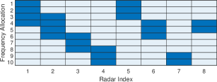
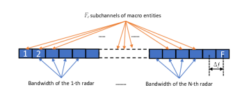
Fig. 3 illustrates the bandwidth shared by radars and communications, where some communications sub-channels partially/completely overlap with those used by radars.
Refer to caption
Figure 3: Illustration of spectrum usage for the HRCN, where each blue block represents the subchannel or subcarriers. The occupied bandwidth of each radar is continuous and pre-allocated.
HRCN interference

During a fusion interval, multiple radar measurements coexist with J𝐽J communications downlinks. Consequently, we have the following cases of interference within the HRCN:

Intra-system interference

As mentioned earlier, there is no intra-tier interference arising from the non-interfering OFDMA resource-block allocation. But spectrum reuse results in cross-tier interference to the micro users. For N𝑁N radars, we do not impose any limitation on the bandwidth overlap. The interference among the N𝑁N radars is assumed to be negligible because all the constituent radars adopt directional beams.

Inter-system interference

This refers to the mutual interference between radars and communications. The coefficients accounting for the interference from the j𝑗j-th macro downlink to the i𝑖i-th radar and from the i𝑖i-th radar to the j𝑗j-th downlink are denoted by αi,jcsuperscriptsubscript𝛼𝑖𝑗𝑐\alpha_{i,j}^{c} and αj,irsuperscriptsubscript𝛼𝑗𝑖𝑟\alpha_{j,i}^{r}, respectively. Both αi,jcsuperscriptsubscript𝛼𝑖𝑗𝑐\alpha_{i,j}^{c} and αj,irsuperscriptsubscript𝛼𝑗𝑖𝑟\alpha_{j,i}^{r} are determined by the spectral overlap. The in-band interference from communications to radar is proportional to the overlap [36]. Thus, αi,jc=α~i,jc(𝒇i,kr)T𝒇j,kcsuperscriptsubscript𝛼𝑖𝑗𝑐superscriptsubscript~𝛼𝑖𝑗𝑐superscriptsuperscriptsubscript𝒇𝑖𝑘𝑟𝑇superscriptsubscript𝒇𝑗𝑘𝑐\alpha_{i,j}^{c}=\tilde{\alpha}_{i,j}^{c}\left(\boldsymbol{f}_{i,k}^{r}\right)^{T}\boldsymbol{f}_{j,k}^{c}, where α~i,jcsuperscriptsubscript~𝛼𝑖𝑗𝑐\tilde{\alpha}_{i,j}^{c} is a constant unrelated to the bandwidth333If the channel is frequency-selective [37], then αi,jc=(𝒇i,kr)T(𝜶~i,jc𝒇j,kc)superscriptsubscript𝛼𝑖𝑗𝑐superscriptsuperscriptsubscript𝒇𝑖𝑘𝑟𝑇direct-productsuperscriptsubscript~𝜶𝑖𝑗𝑐superscriptsubscript𝒇𝑗𝑘𝑐\alpha_{i,j}^{c}=\left(\boldsymbol{f}_{i,k}^{r}\right)^{T}\left(\tilde{\boldsymbol{\alpha}}_{i,j}^{c}\odot\boldsymbol{f}_{j,k}^{c}\right), where the vector 𝜶~i,jcsuperscriptsubscript~𝜶𝑖𝑗𝑐\tilde{\boldsymbol{\alpha}}_{i,j}^{c} represents frequency-selectivity.. Similarly, αj,ir=α~j,ir(𝒇j,kc)T𝒇i,krsuperscriptsubscript𝛼𝑗𝑖𝑟superscriptsubscript~𝛼𝑗𝑖𝑟superscriptsuperscriptsubscript𝒇𝑗𝑘𝑐𝑇superscriptsubscript𝒇𝑖𝑘𝑟\alpha_{j,i}^{r}=\tilde{\alpha}_{j,i}^{r}\left(\boldsymbol{f}_{j,k}^{c}\right)^{T}\boldsymbol{f}_{i,k}^{r}, where α~j,irsuperscriptsubscript~𝛼𝑗𝑖𝑟\tilde{\alpha}_{j,i}^{r} is a constant unrelated to the bandwidth. The mutual interference between the i𝑖i-th radar and the l𝑙l-th micro downlink is analogously defined.

II-B Target tracking model

During the k𝑘k-th fusion interval, the state of target q𝑞q at time ti,q,kmsuperscriptsubscript𝑡𝑖𝑞𝑘𝑚t_{i,q,k}^{m} with m{1,,Mi,q,k}𝑚1subscript𝑀𝑖𝑞𝑘m\in\left\{1,\ldots,M_{i,q,k}\right\} is 𝒔i,q,km=[xi,q,km,x˙i,q,km,yi,q,km,y˙i,q,km]Tsuperscriptsubscript𝒔𝑖𝑞𝑘𝑚superscriptsuperscriptsubscript𝑥𝑖𝑞𝑘𝑚superscriptsubscript˙𝑥𝑖𝑞𝑘𝑚superscriptsubscript𝑦𝑖𝑞𝑘𝑚superscriptsubscript˙𝑦𝑖𝑞𝑘𝑚𝑇\boldsymbol{s}_{i,q,k}^{m}=\left[x_{i,q,k}^{m},\dot{x}_{i,q,k}^{m},y_{i,q,k}^{m},\dot{y}_{i,q,k}^{m}\right]^{T}, where (xi,q,km,yi,q,km)superscriptsubscript𝑥𝑖𝑞𝑘𝑚superscriptsubscript𝑦𝑖𝑞𝑘𝑚\left(x_{i,q,k}^{m},y_{i,q,k}^{m}\right) and (x˙i,q,km,y˙i,q,km)superscriptsubscript˙𝑥𝑖𝑞𝑘𝑚superscriptsubscript˙𝑦𝑖𝑞𝑘𝑚\left(\dot{x}_{i,q,k}^{m},\dot{y}_{i,q,k}^{m}\right) denote target’s position and Doppler velocity, respectively, in Cartesian coordinate system. The state 𝒔tk+1qsuperscriptsubscript𝒔subscript𝑡𝑘1𝑞\boldsymbol{s}_{t_{k+1}}^{q} of the target q𝑞q at fusion time tk+1subscript𝑡𝑘1t_{k+1} is 𝒔tk+1q=[xtk+1q,x˙tk+1q,ytk+1q,y˙tk+1q]Tsuperscriptsubscript𝒔subscript𝑡𝑘1𝑞superscriptsuperscriptsubscript𝑥subscript𝑡𝑘1𝑞superscriptsubscript˙𝑥subscript𝑡𝑘1𝑞superscriptsubscript𝑦subscript𝑡𝑘1𝑞superscriptsubscript˙𝑦subscript𝑡𝑘1𝑞𝑇\boldsymbol{s}_{t_{k+1}}^{q}=\left[x_{t_{k+1}}^{q},\dot{x}_{t_{k+1}}^{q},y_{t_{k+1}}^{q},\dot{y}_{t_{k+1}}^{q}\right]^{T}. The state transition and measurement model is

{𝒔tk+1q=f(𝒔i,q,km,tk+1ti,q,km)+𝜸kq,𝒚i,q,km=h(𝒔i,q,km,i)+𝒘i,q,km,casessuperscriptsubscript𝒔subscript𝑡𝑘1𝑞𝑓superscriptsubscript𝒔𝑖𝑞𝑘𝑚subscript𝑡𝑘1superscriptsubscript𝑡𝑖𝑞𝑘𝑚superscriptsubscript𝜸𝑘𝑞otherwisesuperscriptsubscript𝒚𝑖𝑞𝑘𝑚superscriptsubscript𝒔𝑖𝑞𝑘𝑚𝑖superscriptsubscript𝒘𝑖𝑞𝑘𝑚otherwise\begin{cases}\boldsymbol{s}_{t_{k+1}}^{q}=f\left(\boldsymbol{s}_{i,q,k}^{m},t_{k+1}-t_{i,q,k}^{m}\right)+\boldsymbol{\gamma}_{k}^{q},\\ \boldsymbol{y}_{i,q,k}^{m}=h\left(\boldsymbol{s}_{i,q,k}^{m},i\right)+\boldsymbol{w}_{i,q,k}^{m},\end{cases} (3)

where 𝒔i,q,kmsuperscriptsubscript𝒔𝑖𝑞𝑘𝑚\boldsymbol{s}_{i,q,k}^{m} represents the state of target q𝑞q to radar i𝑖i at the receive time ti,q,kmsuperscriptsubscript𝑡𝑖𝑞𝑘𝑚t_{i,q,k}^{m} with m{1,,Mi,q,k}𝑚1subscript𝑀𝑖𝑞𝑘m\in\left\{1,\ldots,M_{i,q,k}\right\}, f()𝑓f\left(\cdot\right) is the transition function with f(𝒔i,q,km,tk+1ti,q,km)=𝑭kq𝒔i,q,km𝑓superscriptsubscript𝒔𝑖𝑞𝑘𝑚subscript𝑡𝑘1superscriptsubscript𝑡𝑖𝑞𝑘𝑚superscriptsubscript𝑭𝑘𝑞superscriptsubscript𝒔𝑖𝑞𝑘𝑚f\left(\boldsymbol{s}_{i,q,k}^{m},t_{k+1}-t_{i,q,k}^{m}\right)=\boldsymbol{F}_{k}^{q}\boldsymbol{s}_{i,q,k}^{m}, 𝑭kq=[𝑰2𝑻]superscriptsubscript𝑭𝑘𝑞delimited-[]tensor-productsubscript𝑰2𝑻\boldsymbol{F}_{k}^{q}=\left[\boldsymbol{I}_{2}\otimes\boldsymbol{T}\right] with 𝑻=[1tk+1ti,q,km01]𝑻delimited-[]1subscript𝑡𝑘1superscriptsubscript𝑡𝑖𝑞𝑘𝑚01\boldsymbol{T}=\left[\begin{array}[]{cc}1&t_{k+1}-t_{i,q,k}^{m}\\ 0&1\end{array}\right], 𝜸kq𝒩(𝟎,𝚪kq)similar-tosuperscriptsubscript𝜸𝑘𝑞𝒩0superscriptsubscript𝚪𝑘𝑞\boldsymbol{\gamma}_{k}^{q}\sim\mathcal{N}\left(\boldsymbol{0},\boldsymbol{\Gamma}_{k}^{q}\right) represents the process noise, 𝒘i,q,km𝒩(𝟎,𝚺i,q,km)similar-tosuperscriptsubscript𝒘𝑖𝑞𝑘𝑚𝒩0superscriptsubscript𝚺𝑖𝑞𝑘𝑚\boldsymbol{w}_{i,q,k}^{m}\sim\mathcal{N}\left(\boldsymbol{0},\boldsymbol{\Sigma}_{i,q,k}^{m}\right) represents the measurement error, and

h(𝒔i,q,km,i)=[Ri,q,kmθi,q,kmνi,q,km]=[(xi,q,kmxi)2+(yi,q,kmyi)2arctan[yi,q,kmyixi,q,kmxi](xi,q,kmxi)x˙tk+1q+(yi,q,kmyi)y˙i,q,km(xi,q,kmxi)2+(yi,q,kmyi)2],superscriptsubscript𝒔𝑖𝑞𝑘𝑚𝑖delimited-[]superscriptsubscript𝑅𝑖𝑞𝑘𝑚superscriptsubscript𝜃𝑖𝑞𝑘𝑚superscriptsubscript𝜈𝑖𝑞𝑘𝑚delimited-[]superscriptsuperscriptsubscript𝑥𝑖𝑞𝑘𝑚subscript𝑥𝑖2superscriptsuperscriptsubscript𝑦𝑖𝑞𝑘𝑚subscript𝑦𝑖2superscriptsubscript𝑦𝑖𝑞𝑘𝑚subscript𝑦𝑖superscriptsubscript𝑥𝑖𝑞𝑘𝑚subscript𝑥𝑖superscriptsubscript𝑥𝑖𝑞𝑘𝑚subscript𝑥𝑖superscriptsubscript˙𝑥subscript𝑡𝑘1𝑞superscriptsubscript𝑦𝑖𝑞𝑘𝑚subscript𝑦𝑖superscriptsubscript˙𝑦𝑖𝑞𝑘𝑚superscriptsuperscriptsubscript𝑥𝑖𝑞𝑘𝑚subscript𝑥𝑖2superscriptsuperscriptsubscript𝑦𝑖𝑞𝑘𝑚subscript𝑦𝑖2\footnotesize{h\left(\boldsymbol{s}_{i,q,k}^{m},i\right)=\left[\begin{array}[]{c}R_{i,q,k}^{m}\\ \theta_{i,q,k}^{m}\\ \nu_{i,q,k}^{m}\end{array}\right]=\left[\begin{array}[]{c}\sqrt{\left(x_{i,q,k}^{m}-x_{i}\right)^{2}+\left(y_{i,q,k}^{m}-y_{i}\right)^{2}}\\ \arctan\left[\frac{y_{i,q,k}^{m}-y_{i}}{x_{i,q,k}^{m}-x_{i}}\right]\\ \frac{\left(x_{i,q,k}^{m}-x_{i}\right)\dot{x}_{t_{k+1}}^{q}+\left(y_{i,q,k}^{m}-y_{i}\right)\dot{y}_{i,q,k}^{m}}{\sqrt{\left(x_{i,q,k}^{m}-x_{i}\right)^{2}+\left(y_{i,q,k}^{m}-y_{i}\right)^{2}}}\end{array}\right],} (4)

is the measurement function given by (4) with Ri,q,kmsuperscriptsubscript𝑅𝑖𝑞𝑘𝑚R_{i,q,k}^{m}, θi,q,kmsuperscriptsubscript𝜃𝑖𝑞𝑘𝑚\theta_{i,q,k}^{m} and νi,q,kmsuperscriptsubscript𝜈𝑖𝑞𝑘𝑚\nu_{i,q,k}^{m} being the range, AoA and velocity, respectively.

Define 𝚺i,q,km=diag(σRi,q,km2,σθi,q,km2,σνi,q,km2),superscriptsubscript𝚺𝑖𝑞𝑘𝑚diagsuperscriptsubscript𝜎superscriptsubscript𝑅𝑖𝑞𝑘𝑚2superscriptsubscript𝜎superscriptsubscript𝜃𝑖𝑞𝑘𝑚2superscriptsubscript𝜎superscriptsubscript𝜈𝑖𝑞𝑘𝑚2\boldsymbol{\Sigma}_{i,q,k}^{m}=\text{diag}\left(\sigma_{R_{i,q,k}^{m}}^{2},\sigma_{\theta_{i,q,k}^{m}}^{2},\sigma_{\nu_{i,q,k}^{m}}^{2}\right), where σRi,q,km2superscriptsubscript𝜎superscriptsubscript𝑅𝑖𝑞𝑘𝑚2\sigma_{R_{i,q,k}^{m}}^{2}, σθi,q,km2superscriptsubscript𝜎superscriptsubscript𝜃𝑖𝑞𝑘𝑚2\sigma_{\theta_{i,q,k}^{m}}^{2} and σνi,q,km2superscriptsubscript𝜎superscriptsubscript𝜈𝑖𝑞𝑘𝑚2\sigma_{\nu_{i,q,k}^{m}}^{2} are the lower bounds on the MSE error of the corresponding parameters in the subscripts. As per [38, 39],

{σRi,q,km2=j=1Jαi,jcPc,kj+σr,i2Pi,q,kmTi,q,kmηi,q,kmζi2cR,σθi,q,km2=j=1Jαi,jcPc,kj+σr,i2Pi,q,kmTi,q,kmηi,q,kmBi2cθ,σνi,q,km2=j=1Jαi,jcPc,kj+σr,i2Pi,q,kmTi,q,kmηi,q,kmζi2cν,casessuperscriptsubscript𝜎superscriptsubscript𝑅𝑖𝑞𝑘𝑚2absentsuperscriptsubscript𝑗1𝐽superscriptsubscript𝛼𝑖𝑗𝑐superscriptsubscript𝑃𝑐𝑘𝑗superscriptsubscript𝜎𝑟𝑖2superscriptsubscript𝑃𝑖𝑞𝑘𝑚superscriptsubscript𝑇𝑖𝑞𝑘𝑚superscriptsubscript𝜂𝑖𝑞𝑘𝑚superscriptsubscript𝜁𝑖2subscript𝑐𝑅superscriptsubscript𝜎superscriptsubscript𝜃𝑖𝑞𝑘𝑚2absentsuperscriptsubscript𝑗1𝐽superscriptsubscript𝛼𝑖𝑗𝑐superscriptsubscript𝑃𝑐𝑘𝑗superscriptsubscript𝜎𝑟𝑖2superscriptsubscript𝑃𝑖𝑞𝑘𝑚superscriptsubscript𝑇𝑖𝑞𝑘𝑚superscriptsubscript𝜂𝑖𝑞𝑘𝑚superscriptsubscript𝐵𝑖2subscript𝑐𝜃superscriptsubscript𝜎superscriptsubscript𝜈𝑖𝑞𝑘𝑚2absentsuperscriptsubscript𝑗1𝐽superscriptsubscript𝛼𝑖𝑗𝑐superscriptsubscript𝑃𝑐𝑘𝑗superscriptsubscript𝜎𝑟𝑖2superscriptsubscript𝑃𝑖𝑞𝑘𝑚superscriptsubscript𝑇𝑖𝑞𝑘𝑚superscriptsubscript𝜂𝑖𝑞𝑘𝑚superscriptsubscript𝜁𝑖2subscript𝑐𝜈\begin{cases}\sigma_{R_{i,q,k}^{m}}^{2}=&\frac{\sum_{j=1}^{J}\alpha_{i,j}^{c}P_{c,k}^{j}+\sigma_{r,i}^{2}}{P_{i,q,k}^{m}T_{i,q,k}^{m}}\eta_{i,q,k}^{m}\zeta_{i}^{-2}c_{R},\\ \sigma_{\theta_{i,q,k}^{m}}^{2}=&\frac{\sum_{j=1}^{J}\alpha_{i,j}^{c}P_{c,k}^{j}+\sigma_{r,i}^{2}}{P_{i,q,k}^{m}T_{i,q,k}^{m}}\eta_{i,q,k}^{m}B_{i}^{2}c_{\theta},\\ \sigma_{\nu_{i,q,k}^{m}}^{2}=&\frac{\sum_{j=1}^{J}\alpha_{i,j}^{c}P_{c,k}^{j}+\sigma_{r,i}^{2}}{P_{i,q,k}^{m}T_{i,q,k}^{m}}\eta_{i,q,k}^{m}\zeta_{i}^{2}c_{\nu},\end{cases} (5)

where Ti,q,kmsuperscriptsubscript𝑇𝑖𝑞𝑘𝑚T_{i,q,k}^{m} is the dwell time444The dwell time is defined as the product of number of pulses for each measurement and pulsewidth [39]. of radar i𝑖i on target q𝑞q, αi,jcsuperscriptsubscript𝛼𝑖𝑗𝑐\alpha_{i,j}^{c} accounts for the interference coefficient from the j𝑗j-th communications downlink to the i𝑖i-th radar, σr,i2superscriptsubscript𝜎𝑟𝑖2\sigma_{r,i}^{2} is the variance of the noise at the receiver of radar i𝑖i, ηi,q,kmsuperscriptsubscript𝜂𝑖𝑞𝑘𝑚\eta_{i,q,k}^{m} is the radar cross-section of the target q𝑞q to radar i𝑖i at the receive time ti,q,kmsuperscriptsubscript𝑡𝑖𝑞𝑘𝑚t_{i,q,k}^{m}, ζisubscript𝜁𝑖\zeta_{i} and Bisubscript𝐵𝑖B_{i} are the transmit signal bandwidth and the 3dB receive beam width of radar i𝑖i, respectively, and cRsubscript𝑐𝑅c_{R}, cθsubscript𝑐𝜃c_{\theta} and cνsubscript𝑐𝜈c_{\nu} are unrelated constants. Therefore, we rewrite

𝚺i,q,km=j=1Jαi,jcPc,kj+σr,i2Pi,q,kmTi,q,km𝑪i,q,km,superscriptsubscript𝚺𝑖𝑞𝑘𝑚superscriptsubscript𝑗1𝐽superscriptsubscript𝛼𝑖𝑗𝑐superscriptsubscript𝑃𝑐𝑘𝑗superscriptsubscript𝜎𝑟𝑖2superscriptsubscript𝑃𝑖𝑞𝑘𝑚superscriptsubscript𝑇𝑖𝑞𝑘𝑚superscriptsubscript𝑪𝑖𝑞𝑘𝑚\boldsymbol{\Sigma}_{i,q,k}^{m}=\frac{\sum_{j=1}^{J}\alpha_{i,j}^{c}P_{c,k}^{j}+\sigma_{r,i}^{2}}{P_{i,q,k}^{m}T_{i,q,k}^{m}}\boldsymbol{C}_{i,q,k}^{m}, (6)

where 𝑪i,q,kmsuperscriptsubscript𝑪𝑖𝑞𝑘𝑚\boldsymbol{C}_{i,q,k}^{m} is the matrix that contains the above-mentioned parameters.

III Problem Formulation

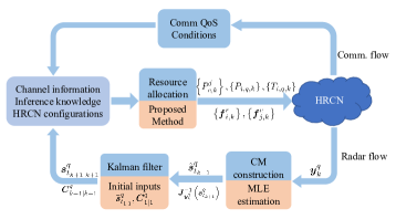
The HRCN configurations presented above indicate that the constituent radars operate in an asynchronous manner. To circumvent the demanding synchronization requirement, we adopt the concept of composition measure (CM), i.e., the CM estimate will serve as the input measurements to the tracking filter [40]. Thus, the estimation accuracy of the CM will determine the tracking performance. It can be gauged from (3)-(6) that the Cramér-Rao bound (CRB) of CM would depend on resources allocated to different entities. Further, the overall filter estimates also depend on these allocations. Here, contrary to [27], our HRCN performance involves the additional dimension of communications which influences resource allocation and impacts CRB derivations.

III-A Composition measure and Bayesian CRB

A composition measure (CM) 𝒔^tk+1qsuperscriptsubscript^𝒔subscript𝑡𝑘1𝑞\hat{\boldsymbol{s}}_{t_{k+1}}^{q} for each target q𝑞q at the fusion time tk+1subscript𝑡𝑘1t_{k+1} is obtained based on all the measurements during the k𝑘k-th fusion interval 𝒚kqsuperscriptsubscript𝒚𝑘𝑞\boldsymbol{y}_{k}^{q}. The CM 𝒔^tk+1qsuperscriptsubscript^𝒔subscript𝑡𝑘1𝑞{\hat{\boldsymbol{s}}_{t_{k+1}}^{q}} is an estimate of the true state 𝒔tk+1qsuperscriptsubscript𝒔subscript𝑡𝑘1𝑞\boldsymbol{s}_{t_{k+1}}^{q} and shown to be statistically efficient even for small sampling sizes [41]. In particular,

𝒚kqsuperscriptsubscript𝒚𝑘𝑞\displaystyle\boldsymbol{y}_{k}^{q} =[(𝒚1,q,k1)T,,(𝒚1,q,kM1,q,k)T,,(𝒚N,q,kMN,q,k)T]T,absentsuperscriptsuperscriptsuperscriptsubscript𝒚1𝑞𝑘1𝑇superscriptsuperscriptsubscript𝒚1𝑞𝑘subscript𝑀1𝑞𝑘𝑇superscriptsuperscriptsubscript𝒚𝑁𝑞𝑘subscript𝑀𝑁𝑞𝑘𝑇𝑇\displaystyle=\left[\left(\boldsymbol{y}_{1,q,k}^{1}\right)^{T},\ldots,\left(\boldsymbol{y}_{1,q,k}^{M_{1,q,k}}\right)^{T},\ldots,\left(\boldsymbol{y}_{N,q,k}^{M_{N,q,k}}\right)^{T}\right]^{T}, (7)
𝒔^tk+1qsuperscriptsubscript^𝒔subscript𝑡𝑘1𝑞\displaystyle\hat{\boldsymbol{s}}_{t_{k+1}}^{q} =[x^tk+1q,x˙^tk+1q,y^tk+1q,y˙^tk+1q]T.absentsuperscriptsuperscriptsubscript^𝑥subscript𝑡𝑘1𝑞superscriptsubscript^˙𝑥subscript𝑡𝑘1𝑞superscriptsubscript^𝑦subscript𝑡𝑘1𝑞superscriptsubscript^˙𝑦subscript𝑡𝑘1𝑞𝑇\displaystyle=\left[\widehat{x}_{t_{k+1}}^{q},\hat{\dot{x}}_{t_{k+1}}^{q},\hat{y}_{t_{k+1}}^{q},\hat{\dot{y}}_{t_{k+1}}^{q}\right]^{T}. (8)

The measurements are independent and the probability density function

p(𝒚kq|𝒔tk+1q)=i=1NmMi,q,k𝒩(h(𝒔i,q,km,i),𝚺i,q,km),𝑝conditionalsuperscriptsubscript𝒚𝑘𝑞superscriptsubscript𝒔subscript𝑡𝑘1𝑞superscriptsubscriptproduct𝑖1𝑁superscriptsubscriptproduct𝑚subscript𝑀𝑖𝑞𝑘𝒩superscriptsubscript𝒔𝑖𝑞𝑘𝑚𝑖superscriptsubscript𝚺𝑖𝑞𝑘𝑚p\left(\boldsymbol{y}_{k}^{q}|{\boldsymbol{s}_{t_{k+1}}^{q}}\right)=\prod_{i=1}^{N}\prod_{m}^{M_{i,q,k}}\mathcal{N}\left(h\left(\boldsymbol{s}_{i,q,k}^{m},i\right),\boldsymbol{\Sigma}_{i,q,k}^{m}\right), (9)

where 𝒔i,q,kmsuperscriptsubscript𝒔𝑖𝑞𝑘𝑚\boldsymbol{s}_{i,q,k}^{m} is predicted based on 𝒔tk+1q=f(𝒔i,q,km,tk+1ti,q,km)superscriptsubscript𝒔subscript𝑡𝑘1𝑞𝑓superscriptsubscript𝒔𝑖𝑞𝑘𝑚subscript𝑡𝑘1superscriptsubscript𝑡𝑖𝑞𝑘𝑚\boldsymbol{s}_{t_{k+1}}^{q}=f\left(\boldsymbol{s}_{i,q,k}^{m},t_{k+1}-t_{i,q,k}^{m}\right). From the maximum likelihood (ML) estimate, the CM is

𝒔^tk+1q=argmax𝒔tk+1q[ln(p(𝒚kq|𝒔tk+1q))].superscriptsubscript^𝒔subscript𝑡𝑘1𝑞superscriptsubscript𝒔subscript𝑡𝑘1𝑞delimited-[]𝑝conditionalsuperscriptsubscript𝒚𝑘𝑞superscriptsubscript𝒔subscript𝑡𝑘1𝑞\hat{\boldsymbol{s}}_{t_{k+1}}^{q}=\underset{{\boldsymbol{s}_{t_{k+1}}^{q}}}{\arg\max}\left[\ln\left(p\left(\boldsymbol{y}_{k}^{q}|{\boldsymbol{s}_{t_{k+1}}^{q}}\right)\right)\right]. (10)

This requires solving a nonlinear least-square problem and the iterated least squares algorithm [42] is usually applied to obtain the ML estimate. Following [27], we approximate the CM covariance matrix by the CRB of 𝒔tk+1qsuperscriptsubscript𝒔subscript𝑡𝑘1𝑞\boldsymbol{s}_{t_{k+1}}^{q} at 𝒔^tk+1qsuperscriptsubscript^𝒔subscript𝑡𝑘1𝑞{\hat{\boldsymbol{s}}_{t_{k+1}}^{q}}. The following Lemma 1 states the Fisher information matrix (FIM) of the true state.

Lemma 1.

The FIM 𝐉𝐲kq(𝐬tk+1q)subscript𝐉superscriptsubscript𝐲𝑘𝑞superscriptsubscript𝐬subscript𝑡𝑘1𝑞\boldsymbol{J}_{\boldsymbol{y}_{k}^{q}}\left(\boldsymbol{s}_{t_{k+1}}^{q}\right) of the target state 𝐬tk+1qsuperscriptsubscript𝐬subscript𝑡𝑘1𝑞\boldsymbol{s}_{t_{k+1}}^{q} is

𝑱𝒚kq(𝒔tk+1q)subscript𝑱superscriptsubscript𝒚𝑘𝑞superscriptsubscript𝒔subscript𝑡𝑘1𝑞\displaystyle\boldsymbol{J}_{\boldsymbol{y}_{k}^{q}}\left(\boldsymbol{s}_{t_{k+1}}^{q}\right) (11)
=\displaystyle= i=1NmMi,q,kPi,q,kmTi,q,kmj=1Jαi,jcPc,kj+σr,i2𝑯i,q,kmT(𝑪i,q,km)1𝑯i,q,km,superscriptsubscript𝑖1𝑁superscriptsubscript𝑚subscript𝑀𝑖𝑞𝑘superscriptsubscript𝑃𝑖𝑞𝑘𝑚superscriptsubscript𝑇𝑖𝑞𝑘𝑚superscriptsubscript𝑗1𝐽superscriptsubscript𝛼𝑖𝑗𝑐superscriptsubscript𝑃𝑐𝑘𝑗superscriptsubscript𝜎𝑟𝑖2superscriptsubscript𝑯𝑖𝑞𝑘𝑚𝑇superscriptsuperscriptsubscript𝑪𝑖𝑞𝑘𝑚1superscriptsubscript𝑯𝑖𝑞𝑘𝑚\displaystyle\sum_{i=1}^{N}\sum_{m}^{M_{i,q,k}}\frac{P_{i,q,k}^{m}T_{i,q,k}^{m}}{\sum_{j=1}^{J}\alpha_{i,j}^{c}P_{c,k}^{j}+\sigma_{r,i}^{2}}\boldsymbol{H}_{i,q,k}^{mT}\left(\boldsymbol{C}_{i,q,k}^{m}\right)^{-1}\boldsymbol{H}_{i,q,k}^{m},

where 𝐇i,q,kmsuperscriptsubscript𝐇𝑖𝑞𝑘𝑚\boldsymbol{H}_{i,q,k}^{m} is the Jacobian of h(𝐬i,q,km,i)superscriptsubscript𝐬𝑖𝑞𝑘𝑚𝑖h\left(\boldsymbol{s}_{i,q,k}^{m},i\right) on 𝐬tk+1qsuperscriptsubscript𝐬subscript𝑡𝑘1𝑞\boldsymbol{s}_{t_{k+1}}^{q} with 𝐬tk+1q=f(𝐬i,q,km,tk+1ti,q,km)superscriptsubscript𝐬subscript𝑡𝑘1𝑞𝑓superscriptsubscript𝐬𝑖𝑞𝑘𝑚subscript𝑡𝑘1superscriptsubscript𝑡𝑖𝑞𝑘𝑚\boldsymbol{s}_{t_{k+1}}^{q}=f\left(\boldsymbol{s}_{i,q,k}^{m},t_{k+1}-t_{i,q,k}^{m}\right).

Proof:

See Appendix -A. ∎

The CM 𝒔^tk+1qsuperscriptsubscript^𝒔subscript𝑡𝑘1𝑞\hat{\boldsymbol{s}}_{t_{k+1}}^{q} and its approximate covariance matrix 𝑱𝒚kq1(𝒔^tk+1q)superscriptsubscript𝑱superscriptsubscript𝒚𝑘𝑞1superscriptsubscript^𝒔subscript𝑡𝑘1𝑞\boldsymbol{J}_{\boldsymbol{y}_{k}^{q}}^{-1}\left(\hat{\boldsymbol{s}}_{t_{k+1}}^{q}\right) are the input to the tracking filter. We denote the filtered estimate by 𝒔~tk+1qsuperscriptsubscript~𝒔subscript𝑡𝑘1𝑞\tilde{\boldsymbol{s}}_{t_{k+1}}^{q}, which is function of 𝒔^tk+1qsuperscriptsubscript^𝒔subscript𝑡𝑘1𝑞\hat{\boldsymbol{s}}_{t_{k+1}}^{q}. The mean-squared error (MSE) of 𝒔tk+1qsuperscriptsubscript𝒔subscript𝑡𝑘1𝑞\boldsymbol{s}_{t_{k+1}}^{q} satisfies the inequality

𝔼𝒚kq[(𝒔~tk+1q𝒔tk+1q)(𝒔~tk+1q𝒔tk+1q)T][𝑩(𝒔tk+1q)]1,succeeds-or-equalssubscript𝔼superscriptsubscript𝒚𝑘𝑞delimited-[]superscriptsubscript~𝒔subscript𝑡𝑘1𝑞superscriptsubscript𝒔subscript𝑡𝑘1𝑞superscriptsuperscriptsubscript~𝒔subscript𝑡𝑘1𝑞superscriptsubscript𝒔subscript𝑡𝑘1𝑞𝑇superscriptdelimited-[]𝑩superscriptsubscript𝒔subscript𝑡𝑘1𝑞1\mathbb{E}_{\boldsymbol{y}_{k}^{q}}\left[\left(\tilde{\boldsymbol{s}}_{t_{k+1}}^{q}-\boldsymbol{s}_{t_{k+1}}^{q}\right)\left(\tilde{\boldsymbol{s}}_{t_{k+1}}^{q}-\boldsymbol{s}_{t_{k+1}}^{q}\right)^{T}\right]\succeq\left[\boldsymbol{B}\left(\boldsymbol{s}_{t_{k+1}}^{q}\right)\right]^{-1}, (12)

where [𝑩(𝒔tk+1q)]1superscriptdelimited-[]𝑩superscriptsubscript𝒔subscript𝑡𝑘1𝑞1\left[\boldsymbol{B}\left(\boldsymbol{s}_{t_{k+1}}^{q}\right)\right]^{-1} is the Bayesian CRB matrix, and 𝑩(𝒔tk+1q)𝑩superscriptsubscript𝒔subscript𝑡𝑘1𝑞\boldsymbol{B}\left(\boldsymbol{s}_{t_{k+1}}^{q}\right) is the corresponding FIM that is adapted from [43] by further incorporating the interference from communications system. These steps produce,

𝑩(𝒔tk+1q)𝑩superscriptsubscript𝒔subscript𝑡𝑘1𝑞\displaystyle\boldsymbol{B}\left(\boldsymbol{s}_{t_{k+1}}^{q}\right) =i=1NmMi,q,kPi,q,kmTi,q,kmj=1Jαi,jcPc,kj+σr,i2𝑪^i,q,km+𝚪~kq,absentsuperscriptsubscript𝑖1𝑁superscriptsubscript𝑚subscript𝑀𝑖𝑞𝑘superscriptsubscript𝑃𝑖𝑞𝑘𝑚superscriptsubscript𝑇𝑖𝑞𝑘𝑚superscriptsubscript𝑗1𝐽superscriptsubscript𝛼𝑖𝑗𝑐superscriptsubscript𝑃𝑐𝑘𝑗superscriptsubscript𝜎𝑟𝑖2superscriptsubscript^𝑪𝑖𝑞𝑘𝑚superscriptsubscript~𝚪𝑘𝑞\displaystyle=\sum_{i=1}^{N}\sum_{m}^{M_{i,q,k}}\frac{P_{i,q,k}^{m}T_{i,q,k}^{m}}{\sum_{j=1}^{J}\alpha_{i,j}^{c}P_{c,k}^{j}+\sigma_{r,i}^{2}}\hat{\boldsymbol{C}}_{i,q,k}^{m}+\tilde{\boldsymbol{\Gamma}}_{k}^{q}, (13)
𝑪^i,q,kmsuperscriptsubscript^𝑪𝑖𝑞𝑘𝑚\displaystyle\hat{\boldsymbol{C}}_{i,q,k}^{m} =𝑯^i,q,kmT(𝑪i,q,km)1𝑯^i,q,km,absentsuperscriptsubscript^𝑯𝑖𝑞𝑘𝑚𝑇superscriptsuperscriptsubscript𝑪𝑖𝑞𝑘𝑚1superscriptsubscript^𝑯𝑖𝑞𝑘𝑚\displaystyle=\hat{\boldsymbol{H}}_{i,q,k}^{mT}\left(\boldsymbol{C}_{i,q,k}^{m}\right)^{-1}\hat{\boldsymbol{H}}_{i,q,k}^{m}, (14)
𝚪~kqsuperscriptsubscript~𝚪𝑘𝑞\displaystyle\tilde{\boldsymbol{\Gamma}}_{k}^{q} =[𝚪kq+𝑭kq𝑩1(𝒔tkq)𝑭kqT]1,absentsuperscriptdelimited-[]superscriptsubscript𝚪𝑘𝑞superscriptsubscript𝑭𝑘𝑞superscript𝑩1superscriptsubscript𝒔subscript𝑡𝑘𝑞superscriptsubscript𝑭𝑘𝑞𝑇1\displaystyle=\left[\boldsymbol{\Gamma}_{k}^{q}+\boldsymbol{F}_{k}^{q}\boldsymbol{B}^{-1}\left(\boldsymbol{s}_{t_{k}}^{q}\right)\boldsymbol{F}_{k}^{qT}\right]^{-1}, (15)

where 𝑯^i,q,kmsuperscriptsubscript^𝑯𝑖𝑞𝑘𝑚\hat{\boldsymbol{H}}_{i,q,k}^{m} is the Jacobian of the measurement at 𝒔¯tk+1|kqsuperscriptsubscript¯𝒔subscript𝑡𝑘conditional1𝑘𝑞\bar{\boldsymbol{s}}_{t_{k+1|k}}^{q} that is the predicted estimate of the true target state.

III-B Resource allocation

To avoid frequent reconfigurations of the system, the allocated power and dwell time from radar i𝑖i on for target q𝑞q are constant over multiple measurements of a fusion interval, i.e.,

{Pi,q,k=Pi,q,k1==Pi,q,kMi,q,k,q=1,,QTi,q,k=Ti,q,k1==Ti,q,kMi,q,k,q=1,,Q.casessubscript𝑃𝑖𝑞𝑘superscriptsubscript𝑃𝑖𝑞𝑘1superscriptsubscript𝑃𝑖𝑞𝑘subscript𝑀𝑖𝑞𝑘for-all𝑞1𝑄subscript𝑇𝑖𝑞𝑘superscriptsubscript𝑇𝑖𝑞𝑘1superscriptsubscript𝑇𝑖𝑞𝑘subscript𝑀𝑖𝑞𝑘for-all𝑞1𝑄\begin{cases}P_{i,q,k}=P_{i,q,k}^{1}=\dots=P_{i,q,k}^{M_{i,q,k}},&\forall q=1,\ldots,Q\\ T_{i,q,k}=T_{i,q,k}^{1}=\dots=T_{i,q,k}^{M_{i,q,k}},&\forall q=1,\ldots,Q.\end{cases} (16)

Recall that the subchannel selection vectors of j𝑗j-th user and i𝑖i-th radar are, respectively,

𝒇j,kcsuperscriptsubscript𝒇𝑗𝑘𝑐\displaystyle\boldsymbol{f}_{j,k}^{c} =[0,,0,1,,1,0,,0]TF×1,j,formulae-sequenceabsentsuperscript001100𝑇superscript𝐹1for-all𝑗\displaystyle=\left[0,\ldots,0,1,\ldots,1,0,\ldots,0\right]^{T}\in\mathbb{R}^{F\times 1},\;\forall j, (17)
𝒇i,krsuperscriptsubscript𝒇𝑖𝑘𝑟\displaystyle\boldsymbol{f}_{i,k}^{r} =[0,,0,1,,1,0,,0]TF×1,i,formulae-sequenceabsentsuperscript001100𝑇superscript𝐹1for-all𝑖\displaystyle=\left[0,\ldots,0,1,\ldots,1,0,\ldots,0\right]^{T}\in\mathbb{R}^{F\times 1},\;\forall i, (18)

where 𝒇i,krsuperscriptsubscript𝒇𝑖𝑘𝑟\boldsymbol{f}_{i,k}^{r} is predefined and fixed over fusion intervals. The vectors {𝒇j,kc}superscriptsubscript𝒇𝑗𝑘𝑐\left\{\boldsymbol{f}_{j,k}^{c}\right\} satisfy the following constraints,

ck={𝟏FT𝒇j,kc=FmincF(𝒇j,kc)T𝒇j^,kc=0,jj^fj,kc0=1,j,superscriptsubscript𝑐𝑘casessuperscriptsubscript1𝐹𝑇superscriptsubscript𝒇𝑗𝑘𝑐superscriptsubscript𝐹𝑚𝑖𝑛𝑐𝐹otherwiseformulae-sequencesuperscriptsuperscriptsubscript𝒇𝑗𝑘𝑐𝑇superscriptsubscript𝒇^𝑗𝑘𝑐0for-all𝑗^𝑗otherwisesubscriptnormsuperscriptsubscript𝑓𝑗𝑘𝑐01for-all𝑗otherwise\mathcal{F}_{c}^{k}=\begin{cases}\boldsymbol{1}_{F}^{T}\boldsymbol{f}_{j,k}^{c}=F_{min}^{c}\leq F\\ \left(\boldsymbol{f}_{j,k}^{c}\right)^{T}\boldsymbol{f}_{\hat{j},k}^{c}=0,\forall j\neq\hat{j}\\ \left\|{f}_{j,k}^{c}\right\|_{0}=1,\forall j,\end{cases} (19)

Based on the above definitions, the bandwidth overlap of the i𝑖i-th radar and the j𝑗j-th user is simply (𝒇i,kr)T𝒇j,kc,i=1,N,j=1,,Jformulae-sequencesuperscriptsuperscriptsubscript𝒇𝑖𝑘𝑟𝑇superscriptsubscript𝒇𝑗𝑘𝑐for-all𝑖1𝑁𝑗1𝐽\left(\boldsymbol{f}_{i,k}^{r}\right)^{T}\boldsymbol{f}_{j,k}^{c},\forall i=1,\ldots N,j=1,\ldots,J. This yields

{αi,jc=α~i,jc(𝒇i,kr)T𝒇j,kcαj,ir=α~j,ir(𝒇i,kr)T𝒇j,kc.casessuperscriptsubscript𝛼𝑖𝑗𝑐superscriptsubscript~𝛼𝑖𝑗𝑐superscriptsuperscriptsubscript𝒇𝑖𝑘𝑟𝑇superscriptsubscript𝒇𝑗𝑘𝑐otherwisesuperscriptsubscript𝛼𝑗𝑖𝑟superscriptsubscript~𝛼𝑗𝑖𝑟superscriptsuperscriptsubscript𝒇𝑖𝑘𝑟𝑇superscriptsubscript𝒇𝑗𝑘𝑐otherwise\begin{cases}\alpha_{i,j}^{c}=\tilde{\alpha}_{i,j}^{c}\left(\boldsymbol{f}_{i,k}^{r}\right)^{T}\boldsymbol{f}_{j,k}^{c}\\ \alpha_{j,i}^{r}=\tilde{\alpha}_{j,i}^{r}\left(\boldsymbol{f}_{i,k}^{r}\right)^{T}\boldsymbol{f}_{j,k}^{c}.\end{cases} (20)

The FIM of the CMs becomes

𝑩(𝒔tk+1q)=i=1NPi,q,kTi,q,kj=1Jα~i,jc(𝒇i,kr)T𝒇j,kcPc,kj+σr,i2𝑪~i,q,k+𝚪~kq,𝑩superscriptsubscript𝒔subscript𝑡𝑘1𝑞superscriptsubscript𝑖1𝑁subscript𝑃𝑖𝑞𝑘subscript𝑇𝑖𝑞𝑘superscriptsubscript𝑗1𝐽superscriptsubscript~𝛼𝑖𝑗𝑐superscriptsuperscriptsubscript𝒇𝑖𝑘𝑟𝑇superscriptsubscript𝒇𝑗𝑘𝑐superscriptsubscript𝑃𝑐𝑘𝑗superscriptsubscript𝜎𝑟𝑖2subscript~𝑪𝑖𝑞𝑘superscriptsubscript~𝚪𝑘𝑞\boldsymbol{B}\left(\boldsymbol{s}_{t_{k+1}}^{q}\right)=\sum_{i=1}^{N}\frac{P_{i,q,k}T_{i,q,k}}{\sum_{j=1}^{J}\tilde{\alpha}_{i,j}^{c}\left(\boldsymbol{f}_{i,k}^{r}\right)^{T}\boldsymbol{f}_{j,k}^{c}P_{c,k}^{j}+\sigma_{r,i}^{2}}\tilde{\boldsymbol{C}}_{i,q,k}+\tilde{\boldsymbol{\Gamma}}_{k}^{q}, (21)

where 𝑪~i,q,k=mMi,q,k𝑪^i,q,kmsubscript~𝑪𝑖𝑞𝑘superscriptsubscript𝑚subscript𝑀𝑖𝑞𝑘superscriptsubscript^𝑪𝑖𝑞𝑘𝑚\tilde{\boldsymbol{C}}_{i,q,k}=\sum_{m}^{M_{i,q,k}}\hat{\boldsymbol{C}}_{i,q,k}^{m}. Hereafter, we use 𝑩(𝒔tk+1q)𝑩superscriptsubscript𝒔subscript𝑡𝑘1𝑞\boldsymbol{B}\left(\boldsymbol{s}_{t_{k+1}}^{q}\right) and 𝑩qsubscript𝑩𝑞\boldsymbol{B}_{q} interchangeably. Note that the diagonal elements of [𝑩(𝒔tk+1q)]1superscriptdelimited-[]𝑩superscriptsubscript𝒔subscript𝑡𝑘1𝑞1\left[\boldsymbol{B}\left(\boldsymbol{s}_{t_{k+1}}^{q}\right)\right]^{-1} are not homogeneous because of different units for distance and velocity. For fair optimization, we normalize them to 𝚲𝑩1(𝒔tk+1q)𝚲T𝚲superscript𝑩1superscriptsubscript𝒔subscript𝑡𝑘1𝑞superscript𝚲𝑇\boldsymbol{\Lambda}\boldsymbol{B}^{-1}\left(\boldsymbol{s}_{t_{k+1}}^{q}\right)\boldsymbol{\Lambda}^{T}, where 𝚲=diag(𝑰2[100T0])𝚲diagtensor-productsubscript𝑰2delimited-[]100subscript𝑇0\boldsymbol{\Lambda}=\text{diag}\left(\boldsymbol{I}_{2}\otimes\left[\begin{array}[]{cc}1&0\\ 0&T_{0}\end{array}\right]\right) is the normalized matrix.

Define the following metric of estimation accuracy

g({Pc,kj},{Pi,q,k},{Ti,q,k},{𝒇j,kc})=q=1Q1Tr(𝚲𝑩q1𝚲T),𝑔superscriptsubscript𝑃𝑐𝑘𝑗subscript𝑃𝑖𝑞𝑘subscript𝑇𝑖𝑞𝑘superscriptsubscript𝒇𝑗𝑘𝑐superscriptsubscript𝑞1𝑄1Tr𝚲subscriptsuperscript𝑩1𝑞superscript𝚲𝑇g\left(\left\{P_{c,k}^{j}\right\},\left\{P_{i,q,k}\right\},\left\{T_{i,q,k}\right\},\left\{\boldsymbol{f}_{j,k}^{c}\right\}\right)=\sum_{q=1}^{Q}\frac{1}{\text{Tr}\left(\boldsymbol{\Lambda}\boldsymbol{B}^{-1}_{q}\boldsymbol{\Lambda}^{T}\right)}, (22)

where Tr(𝚲𝑩1(𝒔tk+1q)𝚲T)Tr𝚲superscript𝑩1superscriptsubscript𝒔subscript𝑡𝑘1𝑞superscript𝚲𝑇\text{Tr}\left(\boldsymbol{\Lambda}\boldsymbol{B}^{-1}\left(\boldsymbol{s}_{t_{k+1}}^{q}\right)\boldsymbol{\Lambda}^{T}\right) accounts for the total MSE error of 𝒔tk+1qsuperscriptsubscript𝒔subscript𝑡𝑘1𝑞\boldsymbol{s}_{t_{k+1}}^{q}. Therefore, maximizing this metric will lead to reduction in the MSE for each target estimate.

Based on (1), the j𝑗j-th macro throughput, j=1,,Jfor-all𝑗1𝐽\forall j=1,\ldots,J, is r({Pc,kj},{Pi,q,k},{Ti,q,k},{𝒇j,kc})=log(1+βjPc,kjT0i=1Nq=1QMi,q,kα~j,irPi,q,kTi,q,k𝒇i,krT𝒇j,kc+σc,j2T0)𝑟superscriptsubscript𝑃𝑐𝑘𝑗subscript𝑃𝑖𝑞𝑘subscript𝑇𝑖𝑞𝑘superscriptsubscript𝒇𝑗𝑘𝑐1superscript𝛽𝑗superscriptsubscript𝑃𝑐𝑘𝑗subscript𝑇0superscriptsubscript𝑖1𝑁superscriptsubscript𝑞1𝑄subscript𝑀𝑖𝑞𝑘superscriptsubscript~𝛼𝑗𝑖𝑟subscript𝑃𝑖𝑞𝑘subscript𝑇𝑖𝑞𝑘superscriptsubscript𝒇𝑖𝑘𝑟𝑇superscriptsubscript𝒇𝑗𝑘𝑐superscriptsubscript𝜎𝑐𝑗2subscript𝑇0r\left(\left\{P_{c,k}^{j}\right\},\left\{P_{i,q,k}\right\},\left\{T_{i,q,k}\right\},\left\{\boldsymbol{f}_{j,k}^{c}\right\}\right)=\text{$\log$}\left(1+\frac{\beta^{j}P_{c,k}^{j}T_{0}}{\sum_{i=1}^{N}\sum_{q=1}^{Q}M_{i,q,k}\tilde{\alpha}_{j,i}^{r}P_{i,q,k}T_{i,q,k}\boldsymbol{f}_{i,k}^{rT}\boldsymbol{f}_{j,k}^{c}+\sigma_{c,j}^{2}T_{0}}\right). Similarly, the downlink throughput expression for the l𝑙l-th micro users, l=1,,Lfor-all𝑙1𝐿\forall l=1,\ldots,L, is based on (2).

It is natural to consider both macro and micro throughput in resource allocation for HRCN system. However, this results in a centralized solution to the multi-tier cellular network, which is computationally expensive because of the high cross-tier signaling overhead [35]. Therefore, assuming that the microcell resource is allocated independently within the micro BS, we consider the joint allocation over the radars and the macro BS of the multi-tier cellular network. Without loss of generality, our proposed algorithm is also applicable when the micro user throughput is included with appropriate constraints because of the linearity of interference terms in the denominator of (2). This leads to a two-stage optimization procedure, which could be one-shot or used in a loop; we omit this here and focus on only macroscopic problem.

Define the optimization variables

𝒛k=subscript𝒛𝑘absent\displaystyle\boldsymbol{z}_{k}= [P1,1,k,,PNc,Q,k,TNc+1,1,k,,TNc+Np,Q,k,\displaystyle\left[P_{1,1,k},\ldots,P_{N_{c},Q,k},T_{N_{c}+1,1,k},\ldots,T_{N_{c}+N_{p},Q,k},\right. (23)
Pc,k1,,Pc,kJ]T\displaystyle\left.P_{c,k}^{1},\ldots,P_{c,k}^{J}\right]^{T} (24)
𝑭kcsuperscriptsubscript𝑭𝑘𝑐\displaystyle\boldsymbol{F}_{k}^{c} =[𝒇1,kc,,𝒇J,kc],absentsuperscriptsubscript𝒇1𝑘𝑐superscriptsubscript𝒇𝐽𝑘𝑐\displaystyle=\left[\boldsymbol{f}_{1,k}^{c},\ldots,\boldsymbol{f}_{J,k}^{c}\right], (25)

The resource allocation requires solving the optimization

maximize𝒛k,𝑭kcsubscript𝒛𝑘superscriptsubscript𝑭𝑘𝑐maximize\displaystyle\underset{\boldsymbol{z}_{k},\boldsymbol{F}_{k}^{c}}{\text{maximize}} g(𝒛k,𝑭kc)𝑔subscript𝒛𝑘superscriptsubscript𝑭𝑘𝑐\displaystyle g\left(\boldsymbol{z}_{k},\boldsymbol{F}_{k}^{c}\right) (26)
subject to r(𝒛k,𝑭kc)ϵkj,j𝑟subscript𝒛𝑘superscriptsubscript𝑭𝑘𝑐superscriptsubscriptitalic-ϵ𝑘𝑗for-all𝑗\displaystyle r\left(\boldsymbol{z}_{k},\boldsymbol{F}_{k}^{c}\right)\geq\epsilon_{k}^{j},\forall j
q=1QMi,q,kPi,q,kPtotali,iφcformulae-sequencesuperscriptsubscript𝑞1𝑄subscript𝑀𝑖𝑞𝑘subscript𝑃𝑖𝑞𝑘superscriptsubscript𝑃𝑡𝑜𝑡𝑎𝑙𝑖for-all𝑖subscript𝜑𝑐\displaystyle\sum_{q=1}^{Q}M_{i,q,k}P_{i,q,k}\leq P_{total}^{i},\forall i\in\varphi_{c}
q=1QMi,q,kTi,q,kTtotali,iφpformulae-sequencesuperscriptsubscript𝑞1𝑄subscript𝑀𝑖𝑞𝑘subscript𝑇𝑖𝑞𝑘superscriptsubscript𝑇𝑡𝑜𝑡𝑎𝑙𝑖for-all𝑖subscript𝜑𝑝\displaystyle\sum_{q=1}^{Q}M_{i,q,k}T_{i,q,k}\leq T_{total}^{i},\forall i\in\varphi_{p}
j=1JPc,kjPtotalcsuperscriptsubscript𝑗1𝐽superscriptsubscript𝑃𝑐𝑘𝑗superscriptsubscript𝑃𝑡𝑜𝑡𝑎𝑙𝑐\displaystyle\sum_{j=1}^{J}P_{c,k}^{j}\leq P_{total}^{c}
𝒇j,kcck,j.superscriptsubscript𝒇𝑗𝑘𝑐superscriptsubscript𝑐𝑘for-all𝑗\displaystyle\boldsymbol{f}_{j,k}^{c}\in\mathcal{F}_{c}^{k},\forall j.

In (26), the first constraint represents the throughput requirements on the J𝐽J macro downlinks. The second and third constraints, respectively, account for radar’s power and dwell time budgets. The last two constraints represent the budgets of communications power and bandwidth, respectively. This is a general formulation that subsumes the problem in [27] as a special case when only radar’s power and dwell time are considered. For the sake of simplicity, we considered only the macro users. However, the problem can be easily extended to micro users and, importantly, our proposed ANCHOR algorithm is still applicable. Overall, the problem is highly challenging because the objective function as well as some constraints are non-convex; variables 𝒛ksubscript𝒛𝑘\boldsymbol{z}_{k} and 𝑭kcsuperscriptsubscript𝑭𝑘𝑐\boldsymbol{F}_{k}^{c} are coupled; and constraints on 𝑭kcsuperscriptsubscript𝑭𝑘𝑐\boldsymbol{F}_{k}^{c} imply a mixed-integer programming.

IV Optimization Method for Resource Allocation

We now develop an algorithm to solve (26) of the k𝑘k-th fusion interval and, for notational simplicity, we omit the subscript k𝑘k hereafter. We employ the alternating optimization to decouple the optimization for 𝒛𝒛\boldsymbol{z} and 𝑭csuperscript𝑭𝑐\boldsymbol{F}^{c}; this corresponds to an alternating update of the binary frequency allocation and the continuous power and dwell time allocation.

IV-A Frequency allocation

For a fixed 𝒛subscript𝒛\boldsymbol{z}_{\ell} at the \ell-th iteration, the subproblem of optimizing 𝑭csuperscript𝑭𝑐\boldsymbol{F}^{c} in problem (26) is

maximize𝑭csuperscript𝑭𝑐maximize\displaystyle\underset{\boldsymbol{F}^{c}}{\text{maximize}} q=1Q1Tr(𝚲𝑩q1𝚲T)superscriptsubscript𝑞1𝑄1Tr𝚲superscriptsubscript𝑩𝑞1superscript𝚲𝑇\displaystyle\sum_{q=1}^{Q}\frac{1}{\text{Tr}\left(\boldsymbol{\Lambda}\boldsymbol{B}_{q}^{-1}\boldsymbol{\Lambda}^{T}\right)} (27)
subject to 𝒂jT𝒇jcϵ~j,jsuperscriptsubscript𝒂𝑗𝑇superscriptsubscript𝒇𝑗𝑐superscript~italic-ϵ𝑗for-all𝑗\displaystyle\boldsymbol{a}_{j}^{T}\boldsymbol{f}_{j}^{c}\leq\tilde{\epsilon}^{j},\forall j
𝒇jcc,j=1,,Jformulae-sequencesuperscriptsubscript𝒇𝑗𝑐subscript𝑐for-all𝑗1𝐽\displaystyle\boldsymbol{f}_{j}^{c}\in\mathcal{F}_{c},\forall j=1,\ldots,J

with

{𝑩q=i=1N𝑪~i,q,kj=1J𝒃i,jT𝒇jc+σ~r,i2+𝚪~kq𝒃i,j=α~i,jcPc,kjPi,q,kTi,q,k𝒇i,kr𝒂j=i=1Nα~j,ir(q=1QMi,qPi,qTi,q)𝒇irσ~r,i2=σr,i2Pi,q,kTi,q,kϵ~j=(βjPc,kjσc,j2(eϵj1))T0eϵj1.casessubscript𝑩𝑞superscriptsubscript𝑖1𝑁subscript~𝑪𝑖𝑞𝑘superscriptsubscript𝑗1𝐽superscriptsubscript𝒃𝑖𝑗𝑇superscriptsubscript𝒇𝑗𝑐superscriptsubscript~𝜎𝑟𝑖2superscriptsubscript~𝚪𝑘𝑞otherwisesubscript𝒃𝑖𝑗superscriptsubscript~𝛼𝑖𝑗𝑐superscriptsubscript𝑃𝑐𝑘𝑗subscript𝑃𝑖𝑞𝑘subscript𝑇𝑖𝑞𝑘superscriptsubscript𝒇𝑖𝑘𝑟otherwisesubscript𝒂𝑗superscriptsubscript𝑖1𝑁superscriptsubscript~𝛼𝑗𝑖𝑟superscriptsubscript𝑞1𝑄subscript𝑀𝑖𝑞subscript𝑃𝑖𝑞subscript𝑇𝑖𝑞superscriptsubscript𝒇𝑖𝑟otherwisesuperscriptsubscript~𝜎𝑟𝑖2superscriptsubscript𝜎𝑟𝑖2subscript𝑃𝑖𝑞𝑘subscript𝑇𝑖𝑞𝑘otherwisesuperscript~italic-ϵ𝑗superscript𝛽𝑗superscriptsubscript𝑃𝑐𝑘𝑗superscriptsubscript𝜎𝑐𝑗2superscript𝑒superscriptitalic-ϵ𝑗1subscript𝑇0superscript𝑒superscriptitalic-ϵ𝑗1otherwise\begin{cases}\boldsymbol{B}_{q}=\sum_{i=1}^{N}\frac{\tilde{\boldsymbol{C}}_{i,q,k}}{\sum_{j=1}^{J}\boldsymbol{b}_{i,j}^{T}\boldsymbol{f}_{j}^{c}+\tilde{\sigma}_{r,i}^{2}}+\tilde{\boldsymbol{\Gamma}}_{k}^{q}\\ \boldsymbol{b}_{i,j}=\frac{\tilde{\alpha}_{i,j}^{c}P_{c,k}^{j}}{P_{i,q,k}T_{i,q,k}}\boldsymbol{f}_{i,k}^{r}\\ \boldsymbol{a}_{j}=\sum_{i=1}^{N}\tilde{\alpha}_{j,i}^{r}\left(\sum_{q=1}^{Q}M_{i,q}P_{i,q}T_{i,q}\right)\boldsymbol{f}_{i}^{r}\\ \tilde{\sigma}_{r,i}^{2}=\frac{\sigma_{r,i}^{2}}{P_{i,q,k}T_{i,q,k}}\\ \tilde{\epsilon}^{j}=\frac{\left(\beta^{j}P_{c,k}^{j}-\sigma_{c,j}^{2}\left(e^{\epsilon^{j}}-1\right)\right)T_{0}}{e^{\epsilon^{j}}-1}.\end{cases} (28)

Considering the special structure of the constraint set csubscript𝑐\mathcal{F}_{c} specified in (19), define 𝒇jc=𝒔j𝟏Fminc,j=1,Jformulae-sequencesuperscriptsubscript𝒇𝑗𝑐multiplicative-conjunctionsubscript𝒔𝑗subscript1superscriptsubscript𝐹𝑚𝑖𝑛𝑐for-all𝑗1𝐽\boldsymbol{f}_{j}^{c}=\boldsymbol{s}_{j}\varotimes\boldsymbol{1}_{F_{min}^{c}},\forall j=1,\ldots J, where 𝒔jsubscript𝒔𝑗\boldsymbol{s}_{j} is a vector of length Nf=FFmincsubscript𝑁𝑓𝐹superscriptsubscript𝐹𝑚𝑖𝑛𝑐N_{f}=\frac{F}{F_{min}^{c}} (clearly, Nfsubscript𝑁𝑓N_{f} is an integer). Thus, problem (27) is equivalently recast into

maximize{𝒔j}subscript𝒔𝑗maximize\displaystyle\underset{\left\{\boldsymbol{s}_{j}\right\}}{\text{maximize}} q=1Q1Tr(𝚲𝑩q1𝚲T)superscriptsubscript𝑞1𝑄1Tr𝚲superscriptsubscript𝑩𝑞1superscript𝚲𝑇\displaystyle\sum_{q=1}^{Q}\frac{1}{\text{Tr}\left(\boldsymbol{\Lambda}\boldsymbol{B}_{q}^{-1}\boldsymbol{\Lambda}^{T}\right)} (29)
subject to 𝒂~jT𝒔jϵ~j,jsuperscriptsubscript~𝒂𝑗𝑇subscript𝒔𝑗superscript~italic-ϵ𝑗for-all𝑗\displaystyle\tilde{\boldsymbol{a}}_{j}^{T}\boldsymbol{s}_{j}\leq\tilde{\epsilon}^{j},\forall j
𝒔j{0,1}Nf×1subscript𝒔𝑗superscript01subscript𝑁𝑓1\displaystyle\boldsymbol{s}_{j}\in\left\{0,1\right\}^{N_{f}\times 1}
𝟏T𝒔j=1,jsuperscript1𝑇subscript𝒔𝑗1for-all𝑗\displaystyle\boldsymbol{1}^{T}\boldsymbol{s}_{j}=1,\forall j
𝒔jT𝒔j^=0,jj^{1,,J},formulae-sequencesuperscriptsubscript𝒔𝑗𝑇subscript𝒔^𝑗0for-all𝑗^𝑗1𝐽\displaystyle\boldsymbol{s}_{j}^{T}\boldsymbol{s}_{\hat{j}}=0,\forall j\neq\hat{j}\in\{1,\ldots,J\},

where 𝑩qsubscript𝑩𝑞\boldsymbol{B}_{q} in (28) is recast as 𝑩q=i=1N𝑪~i,q,kj=1J𝒃~i,jT𝒔j+σ~r,i2+𝚪~kqsubscript𝑩𝑞superscriptsubscript𝑖1𝑁subscript~𝑪𝑖𝑞𝑘superscriptsubscript𝑗1𝐽superscriptsubscript~𝒃𝑖𝑗𝑇subscript𝒔𝑗superscriptsubscript~𝜎𝑟𝑖2superscriptsubscript~𝚪𝑘𝑞\boldsymbol{B}_{q}=\sum_{i=1}^{N}\frac{\tilde{\boldsymbol{C}}_{i,q,k}}{\sum_{j=1}^{J}\tilde{\boldsymbol{b}}_{i,j}^{T}\boldsymbol{s}_{j}+\tilde{\sigma}_{r,i}^{2}}+\tilde{\boldsymbol{\Gamma}}_{k}^{q}, 𝒃~i,j=(𝑰Nf𝟏FmincT)𝒃i,jsubscript~𝒃𝑖𝑗multiplicative-conjunctionsubscript𝑰subscript𝑁𝑓superscriptsubscript1superscriptsubscript𝐹𝑚𝑖𝑛𝑐𝑇subscript𝒃𝑖𝑗\tilde{\boldsymbol{b}}_{i,j}=\left(\boldsymbol{I}_{N_{f}}\varotimes\boldsymbol{1}_{F_{min}^{c}}^{T}\right)\boldsymbol{b}_{i,j}, and 𝒂~j=(𝑰Nf𝟏FmincT)𝒂jsubscript~𝒂𝑗multiplicative-conjunctionsubscript𝑰subscript𝑁𝑓superscriptsubscript1superscriptsubscript𝐹𝑚𝑖𝑛𝑐𝑇subscript𝒂𝑗\tilde{\boldsymbol{a}}_{j}=\left(\boldsymbol{I}_{N_{f}}\varotimes\boldsymbol{1}_{F_{min}^{c}}^{T}\right)\boldsymbol{a}_{j}. Denote the optimal solution of (27) and (29) by (𝒇jc)=𝒔j𝟏Fmincsuperscriptsuperscriptsubscript𝒇𝑗𝑐multiplicative-conjunctionsuperscriptsubscript𝒔𝑗subscript1superscriptsubscript𝐹𝑚𝑖𝑛𝑐\left(\boldsymbol{f}_{j}^{c}\right)^{\star}=\boldsymbol{s}_{j}^{\star}\varotimes\boldsymbol{1}_{F_{min}^{c}} and 𝒔jsuperscriptsubscript𝒔𝑗\boldsymbol{s}_{j}^{\star}, respectively.

The problem in (29) can be interpreted as an assignment problem with a nonlinear objective function. The constraints in (29) indicate that the problem is to assign an exclusive location to the only non-zero element, i.e. 1, for each 𝒔jsubscript𝒔𝑗\boldsymbol{s}_{j} so that the objective value is maximized. For the classical assignment problem, Hungarian method [44] is a classical approach that yields the global optimal solution with a cubic complexity. However, it can only solve for linear objective function. Although many subsequent works extend it to the nonlinear cases, most of them are heuristic and only available to bilinear, quadratic, biquadratic, and cubic objectives [45]. The objective function of problem (29) does not belong to any of the above-mentioned classes. Consequently, prior approaches to the nonlinear assignment problems are inapplicable here.

Since the number of feasible assignments is finite, an exhaustive search over the whole feasible space can always yield the optimal solution in polynomial time. However, for large Nfsubscript𝑁𝑓N_{f}, this approach suffers from heavy computations. Here, simulated annealing method offers a trade-off between computational load and optimality while solving (29). In traditional simulated annealing, computational time and complexity are dictated by the exploration/exploitation mechanism and the termination criteria potentially leading to global optimum. However, in the current setting, fewer and faster computations are preferred and hence, in the sequel, we adapt the classical simulated annealing to account for these constraints.

State Transition

Note that in problem (29), each 𝒔jsubscript𝒔𝑗\boldsymbol{s}_{j} should satisfy the constraints

{𝒂~jT𝒔jϵ~j,j𝒔j{0,1}Nf×1.casessuperscriptsubscript~𝒂𝑗𝑇subscript𝒔𝑗superscript~italic-ϵ𝑗for-all𝑗otherwisesubscript𝒔𝑗superscript01subscript𝑁𝑓1otherwise\begin{cases}\tilde{\boldsymbol{a}}_{j}^{T}\boldsymbol{s}_{j}\leq\tilde{\epsilon}^{j},\forall j\\ \boldsymbol{s}_{j}\in\left\{0,1\right\}^{N_{f}\times 1}.\end{cases} (30)

The corresponding 𝒔^jNf×1,j=1,,Jformulae-sequencesubscript^𝒔𝑗superscriptsubscript𝑁𝑓1for-all𝑗1𝐽\hat{\boldsymbol{s}}_{j}\in\mathbb{R}^{N_{f}\times 1},\forall j=1,\ldots,J is

[𝒔^j]n={0,[𝒂~j]n>ϵ~j1,[𝒂~j]nϵ~j,subscriptdelimited-[]subscript^𝒔𝑗𝑛cases0subscriptdelimited-[]subscript~𝒂𝑗𝑛superscript~italic-ϵ𝑗1subscriptdelimited-[]subscript~𝒂𝑗𝑛superscript~italic-ϵ𝑗\left[\hat{\boldsymbol{s}}_{j}\right]_{n}=\begin{cases}0,&\left[\tilde{\boldsymbol{a}}_{j}\right]_{n}>\tilde{\epsilon}^{j}\\ 1,&\left[\tilde{\boldsymbol{a}}_{j}\right]_{n}\leq\tilde{\epsilon}^{j},\end{cases} (31)

where []nsubscriptdelimited-[]𝑛\left[\cdot\right]_{n} represents the n𝑛n-th element of a vector. Thus, a feasible 𝒔jsubscript𝒔𝑗\boldsymbol{s}_{j} is generated by selecting one nonzero position from 𝒔^jsubscript^𝒔𝑗\hat{\boldsymbol{s}}_{j}. Through this generation approach, the original searching space is reduced. Accordingly, we propose state transform (i.e. moving from the current {𝒔j}subscript𝒔𝑗\left\{\boldsymbol{s}_{j}\right\} to a neighbor) in Algorithm 1. This problem-specific state transition enables faster neighbourhood discovery within the feasible set.

Algorithm 1 Scheme of state transition
1:𝒥={1,,J}𝒥1𝐽\mathcal{J}=\left\{1,\ldots,J\right\}, {𝒔j}subscript𝒔𝑗\left\{\boldsymbol{s}_{j}\right\}, {𝒔^j}subscript^𝒔𝑗\left\{\hat{\boldsymbol{s}}_{j}\right\}
2:{𝒔j}subscript𝒔𝑗\left\{\boldsymbol{s}_{j}\right\}
3:Randomly select j^𝒥^𝑗𝒥\hat{j}\in\mathcal{J}
4:𝒩{n|[𝒔^j^]n>0}𝒩conditional-set𝑛subscriptdelimited-[]subscript^𝒔^𝑗𝑛0\mathcal{N}\leftarrow\left\{n|\left[\hat{\boldsymbol{s}}_{\hat{j}}\right]_{n}>0\right\}
5:while 𝒩𝒩\mathcal{N}\neq\emptyset do
6:     Randomly select n^𝒩^𝑛𝒩\hat{n}\in\mathcal{N} as the nonzero location of 𝒔j^subscript𝒔^𝑗\boldsymbol{s}_{\hat{j}}
7:     𝒩𝒩\n^𝒩\𝒩^𝑛\mathcal{N}\leftarrow\mathcal{N\backslash}\hat{n}
8:     if 𝒔j^T𝒔j=0,j𝒥\j^formulae-sequencesuperscriptsubscript𝒔^𝑗𝑇subscript𝒔𝑗0for-all𝑗\𝒥^𝑗\boldsymbol{s}_{\hat{j}}^{T}\boldsymbol{s}_{j}=0,\forall j\in\mathcal{J}\backslash\hat{j}  then
9:         Exit
10:     end if
11:end while
12:Define j¯¯𝑗\bar{j} be the index associated with 𝒔j^T𝒔j¯0superscriptsubscript𝒔^𝑗𝑇subscript𝒔¯𝑗0\boldsymbol{s}_{\hat{j}}^{T}\boldsymbol{s}_{\bar{j}}\neq 0
13:j^j¯^𝑗¯𝑗\hat{j}\leftarrow\bar{j} and go to Line 3
Optimality requirement

Denote the state transition in Algorithm 1 by ()\mathcal{H}\left(\cdot\right) and combine it with the simulated annealing algorithm summarized in Algorithm 2. Note that the simulated annealing , as a global optimization approach, has the theoretical guarantee of convergence in the probabilistic sense [46]. However, the convergence cannot be guaranteed for a specific run/instance. Algorithm 2 is a nested component of the alternating optimization framework. So, it is viable to terminate the iterations of the algorithm as long as the objective function of problem (27) improves over the previous iteration. This mitigates the demanding requirement on the simulated-annealing-based algorithm to find a global optimum while offering the designer a flexibility in the selection of the termination criterion.

Algorithm 2 Global optimal search for frequency allocation
1:{𝒃^j},{δj},{𝒂^i,j},Tmax,Tmin,δTsubscript^𝒃𝑗subscript𝛿𝑗subscript^𝒂𝑖𝑗subscript𝑇maxsubscript𝑇min𝛿𝑇\left\{\hat{\boldsymbol{b}}_{j}\right\},\left\{\delta_{j}\right\},\left\{\hat{\boldsymbol{a}}_{i,j}\right\},T_{\text{max}},T_{\text{min}},\delta T
2:{𝒔j}subscript𝒔𝑗\left\{\boldsymbol{s}_{j}\right\}
3:TTmax𝑇subscript𝑇maxT\leftarrow T_{\text{max}}
4:while TTmin𝑇subscript𝑇minT\geq T_{\text{min}} do
5:     𝑩qi=1N𝑪~i,q,kj=1J𝒃~i,jT𝒔j+σ~r,i2+𝚪~kqsubscript𝑩𝑞superscriptsubscript𝑖1𝑁subscript~𝑪𝑖𝑞𝑘superscriptsubscript𝑗1𝐽superscriptsubscript~𝒃𝑖𝑗𝑇subscriptsuperscript𝒔𝑗superscriptsubscript~𝜎𝑟𝑖2superscriptsubscript~𝚪𝑘𝑞\boldsymbol{B}_{q}\leftarrow\sum_{i=1}^{N}\frac{\tilde{\boldsymbol{C}}_{i,q,k}}{\sum_{j=1}^{J}\tilde{\boldsymbol{b}}_{i,j}^{T}\boldsymbol{s}^{{}^{\prime}}_{j}+\tilde{\sigma}_{r,i}^{2}}+\tilde{\boldsymbol{\Gamma}}_{k}^{q}
6:     OBJ1q=1Q1Tr(𝚲𝑩q1𝚲T)subscriptOBJ1superscriptsubscript𝑞1𝑄1Tr𝚲superscriptsubscript𝑩𝑞1superscript𝚲𝑇\text{OBJ}_{1}\leftarrow\sum_{q=1}^{Q}\frac{1}{\text{Tr}\left(\boldsymbol{\Lambda}\boldsymbol{B}_{q}^{-1}\boldsymbol{\Lambda}^{T}\right)}
7:     {𝒔j}({𝒔j})superscriptsubscript𝒔𝑗subscript𝒔𝑗\left\{\boldsymbol{s}_{j}^{\prime}\right\}\leftarrow\mathcal{H}\left(\left\{\boldsymbol{s}_{j}\right\}\right)
8:     𝑩qi=1N𝑪~i,q,kj=1J𝒃~i,jT𝒔j+σ~r,i2+𝚪~kqsubscript𝑩𝑞superscriptsubscript𝑖1𝑁subscript~𝑪𝑖𝑞𝑘superscriptsubscript𝑗1𝐽superscriptsubscript~𝒃𝑖𝑗𝑇subscriptsuperscript𝒔𝑗superscriptsubscript~𝜎𝑟𝑖2superscriptsubscript~𝚪𝑘𝑞\boldsymbol{B}_{q}\leftarrow\sum_{i=1}^{N}\frac{\tilde{\boldsymbol{C}}_{i,q,k}}{\sum_{j=1}^{J}\tilde{\boldsymbol{b}}_{i,j}^{T}\boldsymbol{s}^{{}^{\prime}}_{j}+\tilde{\sigma}_{r,i}^{2}}+\tilde{\boldsymbol{\Gamma}}_{k}^{q}
9:     OBJ2q=1Q1Tr(𝚲𝑩q1𝚲T)subscriptOBJ2superscriptsubscript𝑞1𝑄1Tr𝚲superscriptsubscript𝑩𝑞1superscript𝚲𝑇\text{OBJ}_{2}\leftarrow\sum_{q=1}^{Q}\frac{1}{\text{Tr}\left(\boldsymbol{\Lambda}\boldsymbol{B}_{q}^{-1}\boldsymbol{\Lambda}^{T}\right)}
10:     ΔOBJ2OBJ1ΔsubscriptOBJ2subscriptOBJ1\Delta\leftarrow\text{OBJ}_{2}-\text{OBJ}_{1}
11:     if Δ>0Δ0\Delta>0 then
12:         {𝒔j}{𝒔j}subscript𝒔𝑗superscriptsubscript𝒔𝑗\left\{\boldsymbol{s}_{j}\right\}\leftarrow\left\{\boldsymbol{s}_{j}^{\prime}\right\}
13:     else if eΔT>rand(0,1)superscript𝑒Δ𝑇rand01e^{\frac{\Delta}{T}}>\text{rand}\left(0,1\right) then
14:         {𝒔j}{𝒔j}subscript𝒔𝑗superscriptsubscript𝒔𝑗\left\{\boldsymbol{s}_{j}\right\}\leftarrow\left\{\boldsymbol{s}_{j}^{\prime}\right\}
15:     end if
16:     TTδT𝑇𝑇𝛿𝑇T\leftarrow T-\delta T
17:end while

IV-B Power and time allocation

To allocate power and time-slots, we adopt the alternating ascent-descent method.

IV-B1 Maximin reformulation

For a fixed 𝑭+1csuperscriptsubscript𝑭1𝑐\boldsymbol{F}_{\ell+1}^{c}, the subproblem of optimizing 𝒛𝒛\boldsymbol{z} is

maximize𝒛𝒛maximize\displaystyle\underset{\boldsymbol{z}}{\text{maximize}} g(𝒛,𝑭+1c)𝑔𝒛superscriptsubscript𝑭1𝑐\displaystyle g\left(\boldsymbol{z},\boldsymbol{F}_{\ell+1}^{c}\right) (32)
subject to r(𝒛,𝑭+1c)ϵj,j;q=1QMi,qPi,qPtotali,iφcformulae-sequence𝑟𝒛superscriptsubscript𝑭1𝑐superscriptitalic-ϵ𝑗for-all𝑗formulae-sequencesuperscriptsubscript𝑞1𝑄subscript𝑀𝑖𝑞subscript𝑃𝑖𝑞superscriptsubscript𝑃𝑡𝑜𝑡𝑎𝑙𝑖for-all𝑖subscript𝜑𝑐\displaystyle r\left(\boldsymbol{z},\boldsymbol{F}_{\ell+1}^{c}\right)\geq\epsilon^{j},\forall j;\;\sum_{q=1}^{Q}M_{i,q}P_{i,q}\leq P_{total}^{i},\forall i\in\varphi_{c}
q=1QMi,qTi,qTtotali,iφp;j=1JPcjPtotalc.formulae-sequencesuperscriptsubscript𝑞1𝑄subscript𝑀𝑖𝑞subscript𝑇𝑖𝑞superscriptsubscript𝑇𝑡𝑜𝑡𝑎𝑙𝑖formulae-sequencefor-all𝑖subscript𝜑𝑝superscriptsubscript𝑗1𝐽superscriptsubscript𝑃𝑐𝑗superscriptsubscript𝑃𝑡𝑜𝑡𝑎𝑙𝑐\displaystyle\sum_{q=1}^{Q}M_{i,q}T_{i,q}\leq T_{total}^{i},\forall i\in\varphi_{p};\;\sum_{j=1}^{J}P_{c}^{j}\leq P_{total}^{c}.

The following Lemma 2 casts (32) to a more convenient form.

Lemma 2.

Denote a set of slack variables by {𝐕q}q=1Qsuperscriptsubscriptsubscript𝐕𝑞𝑞1𝑄\left\{\boldsymbol{V}_{q}\right\}_{q=1}^{Q}. The problem (26) is equivalent to

max𝒛min{𝑽q}𝒛maxsubscript𝑽𝑞min\displaystyle\begin{aligned} \underset{\boldsymbol{z}}{\mathrm{max}}&\underset{\left\{\boldsymbol{V}_{q}\right\}}{\mathrm{min}}\end{aligned} q=1QTr(𝑽qT𝚲~T𝑩q𝚲~𝑽q)superscriptsubscript𝑞1𝑄Trsuperscriptsubscript𝑽𝑞𝑇superscript~𝚲𝑇subscript𝑩𝑞~𝚲subscript𝑽𝑞\displaystyle\sum_{q=1}^{Q}\mathrm{Tr}\left(\boldsymbol{V}_{q}^{T}\tilde{\boldsymbol{\Lambda}}^{T}\boldsymbol{B}_{q}\tilde{\boldsymbol{\Lambda}}\boldsymbol{V}_{q}\right) (33)
subjecttosubjectto\displaystyle\mathrm{subject}\>\mathrm{to} Tr(𝑽q)=1,qTrsubscript𝑽𝑞1for-all𝑞\displaystyle\mathrm{Tr}\left(\boldsymbol{V}_{q}\right)=1,\forall q
r(𝒛,𝑭+1c)ϵj,j;q=1QMi,qPi,qPtotali,iφcformulae-sequence𝑟𝒛superscriptsubscript𝑭1𝑐superscriptitalic-ϵ𝑗for-all𝑗formulae-sequencesuperscriptsubscript𝑞1𝑄subscript𝑀𝑖𝑞subscript𝑃𝑖𝑞superscriptsubscript𝑃𝑡𝑜𝑡𝑎𝑙𝑖for-all𝑖subscript𝜑𝑐\displaystyle r\left(\boldsymbol{z},\boldsymbol{F}_{\ell+1}^{c}\right)\geq\epsilon^{j},\forall j;\;\sum_{q=1}^{Q}M_{i,q}P_{i,q}\leq P_{total}^{i},\forall i\in\varphi_{c}
q=1QMi,qTi,qTtotali,iφp;j=1JPcjPtotalc,formulae-sequencesuperscriptsubscript𝑞1𝑄subscript𝑀𝑖𝑞subscript𝑇𝑖𝑞superscriptsubscript𝑇𝑡𝑜𝑡𝑎𝑙𝑖formulae-sequencefor-all𝑖subscript𝜑𝑝superscriptsubscript𝑗1𝐽superscriptsubscript𝑃𝑐𝑗superscriptsubscript𝑃𝑡𝑜𝑡𝑎𝑙𝑐\displaystyle\sum_{q=1}^{Q}M_{i,q}T_{i,q}\leq T_{total}^{i},\forall i\in\varphi_{p};\;\sum_{j=1}^{J}P_{c}^{j}\leq P_{total}^{c},

where 𝚲~=𝚲1~𝚲superscript𝚲1\tilde{\boldsymbol{\Lambda}}=\boldsymbol{\Lambda}^{-1}.

Proof:

See Appendix -B. ∎

Clearly, through this reformulation, we get rid of the inverse operation on 𝑩qsubscript𝑩𝑞\boldsymbol{B}_{q}.

IV-B2 Alternating descent-ascent method

For problem (33), we resort to the alternating ascent-decent method, which has been widely applied to solve maximin problems555For a minimax problem, the counterpart is usually called alternating descent-ascent method. and has several variants or extensions [47, 48]. The convergence of these methods can be guaranteed under some mild conditions. For more details, we refer the interested reader to [49, 50].

At the n𝑛n-th iteration of the alternating ascent-descent method, given a fixed 𝒛nsuperscript𝒛𝑛\boldsymbol{z}^{n}, the inner minimization problem of {𝑽q}subscript𝑽𝑞\left\{\boldsymbol{V}_{q}\right\} has the closed form solution

𝑽qn+1=(𝚲~T𝑩q,n𝚲~)1Tr[(𝚲~T𝑩q,n𝚲~)1],q=1,,Q,formulae-sequencesuperscriptsubscript𝑽𝑞𝑛1superscriptsuperscript~𝚲𝑇superscriptsubscript𝑩𝑞𝑛~𝚲1Trdelimited-[]superscriptsuperscript~𝚲𝑇superscriptsubscript𝑩𝑞𝑛~𝚲1for-all𝑞1𝑄\boldsymbol{V}_{q}^{n+1}=\frac{\left(\tilde{\boldsymbol{\Lambda}}^{T}\boldsymbol{B}_{q}^{\ell,n}\tilde{\boldsymbol{\Lambda}}\right)^{-1}}{\text{Tr}\left[\left(\tilde{\boldsymbol{\Lambda}}^{T}\boldsymbol{B}_{q}^{\ell,n}\tilde{\boldsymbol{\Lambda}}\right)^{-1}\right]},\;\forall q=1,\ldots,Q, (34)

where 𝑩q,nsuperscriptsubscript𝑩𝑞𝑛\boldsymbol{B}_{q}^{\ell,n} is obtained by substituting 𝑭+1csuperscriptsubscript𝑭1𝑐\boldsymbol{F}_{\ell+1}^{c} and 𝒛nsuperscript𝒛𝑛\boldsymbol{z}^{n} into (21).

For the fixed {𝑽qn+1}superscriptsubscript𝑽𝑞𝑛1\left\{\boldsymbol{V}_{q}^{n+1}\right\}, we have

q=1QTr[(𝚲~𝑽+1q)T𝑩q(𝚲~𝑽+1q)]superscriptsubscript𝑞1𝑄Trdelimited-[]superscript~𝚲superscriptsubscript𝑽1𝑞𝑇subscript𝑩𝑞~𝚲superscriptsubscript𝑽1𝑞\displaystyle\sum_{q=1}^{Q}\text{Tr}\left[\left(\tilde{\boldsymbol{\Lambda}}\boldsymbol{V}_{\ell+1}^{q}\right)^{T}\boldsymbol{B}_{q}\left(\tilde{\boldsymbol{\Lambda}}\boldsymbol{V}_{\ell+1}^{q}\right)\right] (35)
=\displaystyle= i=1Nq=1Qωi,qnPi,qTi,q(𝒇ir)T(j=1Jα~i,jc𝒇j,cPcj)+σr,i2+constant,superscriptsubscript𝑖1𝑁superscriptsubscript𝑞1𝑄superscriptsubscript𝜔𝑖𝑞𝑛subscript𝑃𝑖𝑞subscript𝑇𝑖𝑞superscriptsuperscriptsubscript𝒇𝑖𝑟𝑇superscriptsubscript𝑗1𝐽superscriptsubscript~𝛼𝑖𝑗𝑐superscriptsubscript𝒇𝑗𝑐superscriptsubscript𝑃𝑐𝑗superscriptsubscript𝜎𝑟𝑖2constant\displaystyle\sum_{i=1}^{N}\frac{\sum_{q=1}^{Q}\omega_{i,q}^{n}P_{i,q}T_{i,q}}{\left(\boldsymbol{f}_{i}^{r}\right)^{T}\left(\sum_{j=1}^{J}\tilde{\alpha}_{i,j}^{c}\boldsymbol{f}_{j,\ell}^{c}P_{c}^{j}\right)+\sigma_{r,i}^{2}}+\textrm{constant},

where ωi,qn=Tr[(𝚲~𝑽qn+1)T𝑪~i,q(𝚲~𝑽qn+1)]0superscriptsubscript𝜔𝑖𝑞𝑛Trdelimited-[]superscript~𝚲superscriptsubscript𝑽𝑞𝑛1𝑇subscript~𝑪𝑖𝑞~𝚲superscriptsubscript𝑽𝑞𝑛10\omega_{i,q}^{n}=\text{Tr}\left[\left(\tilde{\boldsymbol{\Lambda}}\boldsymbol{V}_{q}^{n+1}\right)^{T}\tilde{\boldsymbol{C}}_{i,q}\left(\tilde{\boldsymbol{\Lambda}}\boldsymbol{V}_{q}^{n+1}\right)\right]\geq 0, and the constant term is unrelated to 𝒛𝒛\boldsymbol{z}. Thus, the maximization problem of 𝒛𝒛\boldsymbol{z} becomes

maximize𝒛𝒛maximize\displaystyle\underset{\boldsymbol{z}}{\text{maximize}} i=1Nq=1Qωi,qnPi,qTi,q(𝒇ir)T(j=1Jα~i,jc𝒇j,+1cPcj)+σr,i2superscriptsubscript𝑖1𝑁superscriptsubscript𝑞1𝑄superscriptsubscript𝜔𝑖𝑞𝑛subscript𝑃𝑖𝑞subscript𝑇𝑖𝑞superscriptsuperscriptsubscript𝒇𝑖𝑟𝑇superscriptsubscript𝑗1𝐽superscriptsubscript~𝛼𝑖𝑗𝑐superscriptsubscript𝒇𝑗1𝑐superscriptsubscript𝑃𝑐𝑗superscriptsubscript𝜎𝑟𝑖2\displaystyle\sum_{i=1}^{N}\frac{\sum_{q=1}^{Q}\omega_{i,q}^{n}P_{i,q}T_{i,q}}{\left(\boldsymbol{f}_{i}^{r}\right)^{T}\left(\sum_{j=1}^{J}\tilde{\alpha}_{i,j}^{c}\boldsymbol{f}_{j,\ell+1}^{c}P_{c}^{j}\right)+\sigma_{r,i}^{2}} (36)
subject to r(𝒛,𝑭+1c)ϵj,j=1,,Jformulae-sequence𝑟𝒛superscriptsubscript𝑭1𝑐superscriptitalic-ϵ𝑗for-all𝑗1𝐽\displaystyle r\left(\boldsymbol{z},\boldsymbol{F}_{\ell+1}^{c}\right)\geq\epsilon^{j},\forall j=1,\ldots,J
q=1QMi,qPi,qPtotali,iφcformulae-sequencesuperscriptsubscript𝑞1𝑄subscript𝑀𝑖𝑞subscript𝑃𝑖𝑞superscriptsubscript𝑃𝑡𝑜𝑡𝑎𝑙𝑖for-all𝑖subscript𝜑𝑐\displaystyle\sum_{q=1}^{Q}M_{i,q}P_{i,q}\leq P_{total}^{i},\forall i\in\varphi_{c}
q=1QMi,qTi,qTtotali,iφpformulae-sequencesuperscriptsubscript𝑞1𝑄subscript𝑀𝑖𝑞subscript𝑇𝑖𝑞superscriptsubscript𝑇𝑡𝑜𝑡𝑎𝑙𝑖for-all𝑖subscript𝜑𝑝\displaystyle\sum_{q=1}^{Q}M_{i,q}T_{i,q}\leq T_{total}^{i},\forall i\in\varphi_{p}
j=1JPcjPtotalc.superscriptsubscript𝑗1𝐽superscriptsubscript𝑃𝑐𝑗superscriptsubscript𝑃𝑡𝑜𝑡𝑎𝑙𝑐\displaystyle\sum_{j=1}^{J}P_{c}^{j}\leq P_{total}^{c}.

Rewrite the objective function in (36) as

i=1Nq=1Qωi,qnPi,qTi,q(𝒇ir)T(j=1Jα~i,jc𝒇j,+1cPcj)+σr,i2=i=1N𝒄iT𝒛k+di𝒆iT𝒛k+σr,i2,superscriptsubscript𝑖1𝑁superscriptsubscript𝑞1𝑄superscriptsubscript𝜔𝑖𝑞𝑛subscript𝑃𝑖𝑞subscript𝑇𝑖𝑞superscriptsuperscriptsubscript𝒇𝑖𝑟𝑇superscriptsubscript𝑗1𝐽superscriptsubscript~𝛼𝑖𝑗𝑐superscriptsubscript𝒇𝑗1𝑐superscriptsubscript𝑃𝑐𝑗superscriptsubscript𝜎𝑟𝑖2superscriptsubscript𝑖1𝑁superscriptsubscript𝒄𝑖𝑇subscript𝒛𝑘subscript𝑑𝑖superscriptsubscript𝒆𝑖𝑇subscript𝒛𝑘superscriptsubscript𝜎𝑟𝑖2\sum_{i=1}^{N}\frac{\sum_{q=1}^{Q}\omega_{i,q}^{n}P_{i,q}T_{i,q}}{\left(\boldsymbol{f}_{i}^{r}\right)^{T}\left(\sum_{j=1}^{J}\tilde{\alpha}_{i,j}^{c}\boldsymbol{f}_{j,\ell+1}^{c}P_{c}^{j}\right)+\sigma_{r,i}^{2}}=\sum_{i=1}^{N}\frac{\boldsymbol{c}_{i}^{T}\boldsymbol{z}_{k}+d_{i}}{\boldsymbol{e}_{i}^{T}\boldsymbol{z}_{k}+\sigma_{r,i}^{2}}, (37)

where

𝒄i={[0,,0(i1)Q,ωi,1nTi,1,,ωi,QnTi,Q,0,,0(Nc+Npi)Q+J],iφc[0,,0(i1)Q,ωi,1nPi,1,,ωi,QnPi,Q,0,,0(Nc+Npi)Q+J],iφp[0,,0NcQ,0,,0NpQ,0,,0𝐽]iφm,subscript𝒄𝑖cases𝑖1𝑄00superscriptsubscript𝜔𝑖1𝑛subscript𝑇𝑖1superscriptsubscript𝜔𝑖𝑄𝑛subscript𝑇𝑖𝑄subscript𝑁𝑐subscript𝑁𝑝𝑖𝑄𝐽00𝑖subscript𝜑𝑐𝑖1𝑄00superscriptsubscript𝜔𝑖1𝑛subscript𝑃𝑖1superscriptsubscript𝜔𝑖𝑄𝑛subscript𝑃𝑖𝑄subscript𝑁𝑐subscript𝑁𝑝𝑖𝑄𝐽00𝑖subscript𝜑𝑝subscript𝑁𝑐𝑄00subscript𝑁𝑝𝑄00𝐽00𝑖subscript𝜑𝑚\boldsymbol{c}_{i}=\begin{cases}[\underset{\left(i-1\right)Q}{\underbrace{0,\ldots,0}},\omega_{i,1}^{n}T_{i,1},\ldots,\omega_{i,Q}^{n}T_{i,Q},\underset{\left(N_{c}+N_{p}-i\right)Q+J}{\underbrace{0,\ldots,0}}],&i\in\varphi_{c}\\ {}[\underset{\left(i-1\right)Q}{\underbrace{0,\ldots,0}},\omega_{i,1}^{n}P_{i,1},\ldots,\omega_{i,Q}^{n}P_{i,Q},\underset{\left(N_{c}+N_{p}-i\right)Q+J}{\underbrace{0,\ldots,0}}],&i\in\varphi_{p}\\ {}[\underset{N_{c}Q}{\underbrace{0,\ldots,0}},\underset{N_{p}Q}{\underbrace{0,\ldots,0}},\underset{J}{\underbrace{0,\ldots,0}}]&i\in\varphi_{m},\end{cases} (38)
disubscript𝑑𝑖\displaystyle d_{i} ={0,iφc0,iφpq=1Qωi,qPi,qTi,q,iφm,absentcases0𝑖subscript𝜑𝑐0𝑖subscript𝜑𝑝superscriptsubscript𝑞1𝑄superscriptsubscript𝜔𝑖𝑞subscript𝑃𝑖𝑞subscript𝑇𝑖𝑞𝑖subscript𝜑𝑚\displaystyle=\begin{cases}0,&i\in\varphi_{c}\\ 0,&i\in\varphi_{p}\\ \sum_{q=1}^{Q}\omega_{i,q}^{\ell}P_{i,q}T_{i,q},&i\in\varphi_{m},\end{cases} (39)
𝒆isubscript𝒆𝑖\displaystyle\boldsymbol{e}_{i} =[0,,0NcQ,0,,0NpQ\displaystyle=[\underset{N_{c}Q}{\underbrace{0,\ldots,0}},\underset{N_{p}Q}{\underbrace{0,\ldots,0}} (40)
α~i,1cPc1𝒇irT𝒇1,+1c,,α~i,JcPcJ𝒇irT𝒇J,+1c],i.\displaystyle\tilde{\alpha}_{i,1}^{c}P_{c}^{1}\boldsymbol{f}_{i}^{rT}\boldsymbol{f}_{1,\ell+1}^{c},\ldots,\tilde{\alpha}_{i,J}^{c}P_{c}^{J}\boldsymbol{f}_{i}^{rT}\boldsymbol{f}_{J,\ell+1}^{c}],\forall i. (41)

The constraints on 𝒛𝒛\boldsymbol{z} of problem (36) expressed compactly are 𝑨𝒛𝒃𝑨𝒛𝒃\boldsymbol{A}\boldsymbol{z}\leq\boldsymbol{b}, where

𝒃=𝒃absent\displaystyle\boldsymbol{b}= [Ptotal1,PtotalNc,TtotalNc+1,TtotalNc+Np,Ptotalc,\displaystyle\left[P_{total}^{1},\ldots P_{total}^{N_{c}},T_{total}^{N_{c}+1},\ldots T_{total}^{N_{c}+N_{p}},P_{total}^{c},\right. (42)
σc,12T0,,σc,J2T0]T,\displaystyle\left.-\sigma_{c,1}^{2}T_{0},\ldots,-\sigma_{c,J}^{2}T_{0}\right]^{T},

and

𝑨=[𝒎1𝟎𝟎𝟎𝒎Nc+Np𝟎𝟎𝟎𝟏JT𝒏φc1𝒏φp1𝒏c1𝒏φcJ𝒏φpJ𝒏cJ]𝑨delimited-[]subscript𝒎1000subscript𝒎subscript𝑁𝑐subscript𝑁𝑝000superscriptsubscript1𝐽𝑇superscriptsubscript𝒏subscript𝜑𝑐1superscriptsubscript𝒏subscript𝜑𝑝1superscriptsubscript𝒏𝑐1superscriptsubscript𝒏subscript𝜑𝑐𝐽superscriptsubscript𝒏subscript𝜑𝑝𝐽superscriptsubscript𝒏𝑐𝐽\boldsymbol{A}=\left[\begin{array}[]{c}\begin{array}[]{cccc}\boldsymbol{m}_{1}&\boldsymbol{0}&\cdots&\boldsymbol{0}\\ \boldsymbol{0}&\ddots&\ddots&\vdots\\ \vdots&\ddots&\boldsymbol{m}_{N_{c}+N_{p}}&\boldsymbol{0}\\ \boldsymbol{0}&\cdots&\boldsymbol{0}&\boldsymbol{1}_{J}^{T}\end{array}\\ \begin{array}[]{ccc}\boldsymbol{n}_{\varphi_{c}}^{1}&\boldsymbol{n}_{\varphi_{p}}^{1}&\boldsymbol{n}_{c}^{1}\\ \vdots&\vdots&\vdots\\ \boldsymbol{n}_{\varphi_{c}}^{J}&\boldsymbol{n}_{\varphi_{p}}^{J}&\boldsymbol{n}_{c}^{J}\end{array}\end{array}\right] (43)

with

𝒎isubscript𝒎𝑖\displaystyle\boldsymbol{m}_{i} =[Mi,1,,Mi,Q],i=1,,Nc+Np,formulae-sequenceabsentsubscript𝑀𝑖1subscript𝑀𝑖𝑄for-all𝑖1subscript𝑁𝑐subscript𝑁𝑝\displaystyle=\left[M_{i,1},\ldots,M_{i,Q}\right],\forall i=1,\ldots,N_{c}+N_{p}, (44)
𝒏cjsuperscriptsubscript𝒏𝑐𝑗\displaystyle\boldsymbol{n}_{c}^{j} =[0,,0j1,βjT01eϵj,0,,0Jj],j,absent𝑗100superscript𝛽𝑗subscript𝑇01superscript𝑒superscriptitalic-ϵ𝑗𝐽𝑗00for-all𝑗\displaystyle=\left[\underset{j-1}{\underbrace{0,\ldots,0}},\frac{\beta^{j}T_{0}}{1-e^{\epsilon^{j}}},\underset{J-j}{\underbrace{0,\ldots,0}}\right],\forall j, (45)
𝒏φcjsuperscriptsubscript𝒏subscript𝜑𝑐𝑗\displaystyle\boldsymbol{n}_{\varphi_{c}}^{j} =[M1,1α~j,1r𝒇1rT𝒇j,+1cT1,1,\displaystyle=\left[M_{1,1}\tilde{\alpha}_{j,1}^{r}\boldsymbol{f}_{1}^{rT}\boldsymbol{f}_{j,\ell+1}^{c}T_{1,1},\right.
,MNc,Qα~j,Ncr𝒇NcrT𝒇j,+1cTNc,Q],\displaystyle\left.\ldots,M_{N_{c},Q}\tilde{\alpha}_{j,N_{c}}^{r}\boldsymbol{f}_{N_{c}}^{rT}\boldsymbol{f}_{j,\ell+1}^{c}T_{N_{c},Q}\right], (46)
𝒏φpjsuperscriptsubscript𝒏subscript𝜑𝑝𝑗\displaystyle\boldsymbol{n}_{\varphi_{p}}^{j} =[MNc+1,1α~j,Nc+1r𝒇Nc+1rT𝒇j,+1cPNc+1,1,\displaystyle=\left[M_{N_{c}+1,1}\tilde{\alpha}_{j,N_{c}+1}^{r}\boldsymbol{f}_{N_{c}+1}^{rT}\boldsymbol{f}_{j,\ell+1}^{c}P_{N_{c}+1,1},\right.
,MNc+Np,1α~j,Nc+Npr𝒇Nc+NprT𝒇j,+1cPNc+Np,1].\displaystyle\left.\ldots,M_{N_{c}+N_{p},1}\tilde{\alpha}_{j,N_{c}+N_{p}}^{r}\boldsymbol{f}_{N_{c}+N_{p}}^{rT}\boldsymbol{f}_{j,\ell+1}^{c}P_{N_{c}+N_{p},1}\right]. (47)

Therefore, problem (36) is equivalently recast into

maximize𝒛𝒛maximize\displaystyle\underset{\boldsymbol{z}}{\text{maximize}} f(𝒛)i=1N𝒄iT𝒛+di𝒆iT𝒛+σr,i2𝑓𝒛superscriptsubscript𝑖1𝑁superscriptsubscript𝒄𝑖𝑇𝒛subscript𝑑𝑖superscriptsubscript𝒆𝑖𝑇𝒛superscriptsubscript𝜎𝑟𝑖2\displaystyle f\left(\boldsymbol{z}\right)\triangleq\sum_{i=1}^{N}\frac{\boldsymbol{c}_{i}^{T}\boldsymbol{z}+d_{i}}{\boldsymbol{e}_{i}^{T}\boldsymbol{z}+\sigma_{r,i}^{2}} (48)
subject to 𝑨𝒛𝒃,𝒛𝟎,formulae-sequence𝑨𝒛𝒃𝒛0\displaystyle\boldsymbol{A}\boldsymbol{z}\leq\boldsymbol{b},\;\boldsymbol{z}\geq\boldsymbol{0},

which maximizes a sum of linear fractional function over a convex set.

Several methods have been proposed in the literature to solve this fractional programming problem [51, 52, 53, 54]. However, in order to be within the framework of the alternating ascent-descent method, an incremental update on the variable 𝒛𝒛\boldsymbol{z} is necessary. In other words, a global solution to problem (48) might violate the alternating ascent-descent method and its theoretical guarantees. Therefore, within the alternating ascent-descent framework, the update rule of 𝒛𝒛\boldsymbol{z} is simply 𝒛n+1=𝒫𝒵(𝒛n+ηzf(𝒛n))superscript𝒛𝑛1subscript𝒫𝒵superscript𝒛𝑛𝜂subscript𝑧𝑓superscript𝒛𝑛\boldsymbol{z}^{n+1}=\mathcal{P}_{\mathcal{Z}}\left(\boldsymbol{z}^{n}+\eta\nabla_{z}f\left(\boldsymbol{z}^{n}\right)\right), where η𝜂\eta is the stepsize parameter,

zf(𝒛n)=i=1N(𝒆iT𝒛n+σr,i2)𝒄i(𝒄iT𝒛n+di)𝒆i(𝒆iT𝒛n+σr,i2)2,subscript𝑧𝑓superscript𝒛𝑛superscriptsubscript𝑖1𝑁superscriptsubscript𝒆𝑖𝑇superscript𝒛𝑛superscriptsubscript𝜎𝑟𝑖2subscript𝒄𝑖superscriptsubscript𝒄𝑖𝑇superscript𝒛𝑛subscript𝑑𝑖subscript𝒆𝑖superscriptsuperscriptsubscript𝒆𝑖𝑇superscript𝒛𝑛superscriptsubscript𝜎𝑟𝑖22\nabla_{z}f\left(\boldsymbol{z}^{n}\right)=\sum_{i=1}^{N}\frac{\left(\boldsymbol{e}_{i}^{T}\boldsymbol{z}^{n}+\sigma_{r,i}^{2}\right)\boldsymbol{c}_{i}-\left(\boldsymbol{c}_{i}^{T}\boldsymbol{z}^{n}+d_{i}\right)\boldsymbol{e}_{i}}{\left(\boldsymbol{e}_{i}^{T}\boldsymbol{z}^{n}+\sigma_{r,i}^{2}\right)^{2}}, (49)

and 𝒫𝒵()subscript𝒫𝒵\mathcal{P}_{\mathcal{Z}}\left(\cdot\right) represents the projection to the convex set 𝒵={𝒛|𝑨𝒛𝒃,𝒛𝟎}𝒵conditional-set𝒛formulae-sequence𝑨𝒛𝒃𝒛0\mathcal{Z}=\left\{\boldsymbol{z}|\boldsymbol{A}\boldsymbol{z}\leq\boldsymbol{b},\boldsymbol{z}\geq\boldsymbol{0}\right\}, which actually involves solving a convex quadratic problem.

IV-B3 Computational complexity and convergence analysis

The proposed method for the power and time allocation is summarized in Algorithm 3. The overall computational complexity of Algorithm 3 is linear with the number of iterations.

Algorithm 3 Alternating ascent-descent method to power and dwell time allocation
1:{𝑩q},{𝑪~i,q},{Ptotali},{Ttotali},Ptotalc,{Mi,q},𝑭csubscript𝑩𝑞subscript~𝑪𝑖𝑞superscriptsubscript𝑃𝑡𝑜𝑡𝑎𝑙𝑖superscriptsubscript𝑇𝑡𝑜𝑡𝑎𝑙𝑖superscriptsubscript𝑃𝑡𝑜𝑡𝑎𝑙𝑐subscript𝑀𝑖𝑞superscriptsubscript𝑭𝑐\left\{\boldsymbol{B}_{q}\right\},\left\{\tilde{\boldsymbol{C}}_{i,q}\right\},\left\{P_{total}^{i}\right\},\left\{T_{total}^{i}\right\},P_{total}^{c},\left\{M_{i,q}\right\},\boldsymbol{F}_{\ell}^{c}
2:Allocation vector 𝒛𝒛\boldsymbol{z}
3:n0𝑛0n\leftarrow 0
4:initialize a feasible 𝒛nsuperscript𝒛𝑛\boldsymbol{z}^{n}
5:repeat
6:     calculate 𝑩q,nsuperscriptsubscript𝑩𝑞𝑛\boldsymbol{B}_{q}^{\ell,n} by (21)
7:     𝑽qn+1(𝚲~T𝑩q,n𝚲~)1/Tr[(𝚲~T𝑩q,n𝚲~)1]superscriptsubscript𝑽𝑞𝑛1superscriptsuperscript~𝚲𝑇superscriptsubscript𝑩𝑞𝑛~𝚲1Trdelimited-[]superscriptsuperscript~𝚲𝑇superscriptsubscript𝑩𝑞𝑛~𝚲1\boldsymbol{V}_{q}^{n+1}\leftarrow\left(\tilde{\boldsymbol{\Lambda}}^{T}\boldsymbol{B}_{q}^{\ell,n}\tilde{\boldsymbol{\Lambda}}\right)^{-1}/\text{Tr}\left[\left(\tilde{\boldsymbol{\Lambda}}^{T}\boldsymbol{B}_{q}^{\ell,n}\tilde{\boldsymbol{\Lambda}}\right)^{-1}\right]
8:     ωi,qnTr[(𝚲~𝑽qn+1)T𝑪~i,q(𝚲~𝑽qn+1)]superscriptsubscript𝜔𝑖𝑞𝑛Trdelimited-[]superscript~𝚲superscriptsubscript𝑽𝑞𝑛1𝑇subscript~𝑪𝑖𝑞~𝚲superscriptsubscript𝑽𝑞𝑛1\omega_{i,q}^{n}\leftarrow\text{Tr}\left[\left(\tilde{\boldsymbol{\Lambda}}\boldsymbol{V}_{q}^{n+1}\right)^{T}\tilde{\boldsymbol{C}}_{i,q}\left(\tilde{\boldsymbol{\Lambda}}\boldsymbol{V}_{q}^{n+1}\right)\right]
9:     Calculate 𝒄i,di,𝒆i,𝒃,𝑨subscript𝒄𝑖subscript𝑑𝑖subscript𝒆𝑖𝒃𝑨\boldsymbol{c}_{i},d_{i},\boldsymbol{e}_{i},\boldsymbol{b},\boldsymbol{A} by (38), (39), (41), (42) and (43)
10:     zf(𝒛n)i=1N(𝒆iT𝒛n+σr,i2)𝒄i(𝒄iT𝒛n+di)𝒆i(𝒆iT𝒛n+σr,i2)2subscript𝑧𝑓superscript𝒛𝑛superscriptsubscript𝑖1𝑁superscriptsubscript𝒆𝑖𝑇superscript𝒛𝑛superscriptsubscript𝜎𝑟𝑖2subscript𝒄𝑖superscriptsubscript𝒄𝑖𝑇superscript𝒛𝑛subscript𝑑𝑖subscript𝒆𝑖superscriptsuperscriptsubscript𝒆𝑖𝑇superscript𝒛𝑛superscriptsubscript𝜎𝑟𝑖22\nabla_{z}f\left(\boldsymbol{z}^{n}\right)\leftarrow\sum_{i=1}^{N}\frac{\left(\boldsymbol{e}_{i}^{T}\boldsymbol{z}^{n}+\sigma_{r,i}^{2}\right)\boldsymbol{c}_{i}-\left(\boldsymbol{c}_{i}^{T}\boldsymbol{z}^{n}+d_{i}\right)\boldsymbol{e}_{i}}{\left(\boldsymbol{e}_{i}^{T}\boldsymbol{z}^{n}+\sigma_{r,i}^{2}\right)^{2}}
11:     𝒛n+1𝒫𝒵(𝒛n+ηzf(𝒛n))superscript𝒛𝑛1subscript𝒫𝒵superscript𝒛𝑛𝜂subscript𝑧𝑓superscript𝒛𝑛\boldsymbol{z}^{n+1}\leftarrow\mathcal{P}_{\mathcal{Z}}\left(\boldsymbol{z}^{n}+\eta\nabla_{z}f\left(\boldsymbol{z}^{n}\right)\right)
12:     nn+1𝑛𝑛1n\leftarrow n+1
13:until convergence

For the convenience of analysis, we focus on the deterministic cost on a per-iteration basis, which mainly comes from the following sources: 𝑽qn+1superscriptsubscript𝑽𝑞𝑛1\boldsymbol{V}_{q}^{n+1}, ωi,qnsuperscriptsubscript𝜔𝑖𝑞𝑛\omega_{i,q}^{n} and 𝒛n+1superscript𝒛𝑛1\boldsymbol{z}^{n+1}. The computational cost of {𝑽qn+1}superscriptsubscript𝑽𝑞𝑛1\left\{\boldsymbol{V}_{q}^{n+1}\right\} is linear with 𝒪(Q)𝒪𝑄\mathcal{O}\left(Q\right) due to the matrix multiplication and inverse of (𝚲~T𝑩q,n𝚲~)superscript~𝚲𝑇superscriptsubscript𝑩𝑞𝑛~𝚲\left(\tilde{\boldsymbol{\Lambda}}^{T}\boldsymbol{B}_{q}^{\ell,n}\tilde{\boldsymbol{\Lambda}}\right) is a constant. Similarly, the computational of {ωi,qn}superscriptsubscript𝜔𝑖𝑞𝑛\left\{\omega_{i,q}^{n}\right\} is also linear with 𝒪(QN)𝒪𝑄𝑁\mathcal{O}\left(QN\right). The update rule of 𝒛n+1superscript𝒛𝑛1\boldsymbol{z}^{n+1} involves the projection operator 𝒫𝒵()subscript𝒫𝒵\mathcal{P}_{\mathcal{Z}}\left(\cdot\right), which is, in fact, to solve a convex quadratic problem. The MOSEK optimization package will reformulate the problem into epigraph form by introducing an additional slack variable. Consequently, there is a second order cone constraint and the remaining constraints are linear. The computational complexity of solving the reformulated problem is therefore upper bound by 𝒪((NcQ+NpQ+J)3.5)𝒪superscriptsubscript𝑁𝑐𝑄subscript𝑁𝑝𝑄𝐽3.5\mathcal{O}\left(\left(N_{c}Q+N_{p}Q+J\right)^{3.5}\right), the same order as second-order cone programming. The convergence of Algorithm 3 is stated by the following theorem.

Lemma 3.

Assume {𝐳n}superscript𝐳𝑛\left\{\boldsymbol{z}^{n}\right\} to be the generated sequence of Algorithm 3. Then, every limit point of the sequence {𝐳n}superscript𝐳𝑛\left\{\boldsymbol{z}^{n}\right\}is the stationary point of problem (32).

Proof:

See Appendix -C. ∎

The convergence of the combined algorithm ANCHOR to solve problem (26) is stated in the following Lemma 4.

Theorem 4.

Assume that Algorithm 2 outputs an (sub-)optimal solution, then the sequence {g(𝐳,𝐅c)}𝑔subscript𝐳superscriptsubscript𝐅𝑐\left\{g\left(\boldsymbol{z}_{\ell},\boldsymbol{F}_{\ell}^{c}\right)\right\} is non-decreasing and converges to a finite value, where (𝐳,𝐅c)subscript𝐳superscriptsubscript𝐅𝑐\left(\boldsymbol{z}_{\ell},\boldsymbol{F}_{\ell}^{c}\right) is generated by Algorithm 4 at the \ell-th iteration.

Proof:

See Appendix -D. ∎

Algorithm 4 summarizes all steps of ANCHOR.

Algorithm 4 Alternating allocation of heterogeneous resources (ANCHOR)
1:φc,φp,φm,{Ptotali},{Ttotali},Ptotalc,{Mi,q}subscript𝜑𝑐subscript𝜑𝑝subscript𝜑𝑚superscriptsubscript𝑃𝑡𝑜𝑡𝑎𝑙𝑖superscriptsubscript𝑇𝑡𝑜𝑡𝑎𝑙𝑖superscriptsubscript𝑃𝑡𝑜𝑡𝑎𝑙𝑐subscript𝑀𝑖𝑞\varphi_{c},\varphi_{p},\varphi_{m},\left\{P_{total}^{i}\right\},\left\{T_{total}^{i}\right\},P_{total}^{c},\left\{M_{i,q}\right\}
2:Resource allocation vector 𝐳𝐳\mathbf{z}
3:00\ell\leftarrow 0
4:initialize a feasible 𝒛subscript𝒛\boldsymbol{z}_{\ell}
5:repeat
6:     update 𝑭+1csuperscriptsubscript𝑭1𝑐\boldsymbol{F}_{\ell+1}^{c} via Algorithm 2
7:     update 𝒛+1subscript𝒛1\boldsymbol{z}_{\ell+1} via Algorithm 3
8:     +11\ell\leftarrow\ell+1
9:until convergence

IV-C Algorithmic workflow

Refer to caption
Figure 4: Resource allocation procedure for HRCN. The symbols represent either the inputs or outputs of the related modules.

The ANCHOR algorithm is applied to allocate resources for a fusion interval. It is expected that the optimized resource allocation will improve the accuracy of the CM 𝒔^tk+1qsuperscriptsubscript^𝒔subscript𝑡𝑘1𝑞\hat{\boldsymbol{s}}_{t_{k+1}}^{q} and its covariance matrix 𝑱𝒚kq1(𝒔tk+1q)superscriptsubscript𝑱superscriptsubscript𝒚𝑘𝑞1superscriptsubscript𝒔subscript𝑡𝑘1𝑞\boldsymbol{J}_{\boldsymbol{y}_{k}^{q}}^{-1}\left(\boldsymbol{s}_{t_{k+1}}^{q}\right), which further enhances the tracking performance based on Kalman filter. At the k𝑘k-th fusion interval, 𝒔¯tk|kqsuperscriptsubscript¯𝒔subscript𝑡conditional𝑘𝑘𝑞\bar{\boldsymbol{s}}_{t_{k|k}}^{q} is the filtered estimate of the target state 𝒔tkqsuperscriptsubscript𝒔subscript𝑡𝑘𝑞\boldsymbol{s}_{t_{k}}^{q} of the last fusion interval and assumed to be known, and 𝒔^tk+1qsuperscriptsubscript^𝒔subscript𝑡𝑘1𝑞\hat{\boldsymbol{s}}_{t_{k+1}}^{q} is the CM estimated based on the measurements 𝒚kqsuperscriptsubscript𝒚𝑘𝑞\boldsymbol{y}_{k}^{q}. Based on the system model as equation (3), we have

{𝒔¯tk+1|kq=f(𝒔¯tk|kq,T0)𝑪k+1|kq=𝚪kq+𝑭kq𝑪k|kq𝑭kq𝒔¯tk+1|k+1q=𝒔¯tk+1|kq+𝑲k+1q(𝒔^tk+1q𝒔¯tk+1|kq)𝑪k+1|k+1q=(𝑰𝑲k+1q)𝑪k+1|kq,casessuperscriptsubscript¯𝒔subscript𝑡𝑘conditional1𝑘𝑞𝑓superscriptsubscript¯𝒔subscript𝑡conditional𝑘𝑘𝑞subscript𝑇0otherwisesuperscriptsubscript𝑪𝑘conditional1𝑘𝑞superscriptsubscript𝚪𝑘𝑞superscriptsubscript𝑭𝑘𝑞superscriptsubscript𝑪conditional𝑘𝑘𝑞superscriptsubscript𝑭𝑘𝑞otherwisesuperscriptsubscript¯𝒔subscript𝑡𝑘conditional1𝑘1𝑞superscriptsubscript¯𝒔subscript𝑡𝑘conditional1𝑘𝑞superscriptsubscript𝑲𝑘1𝑞superscriptsubscript^𝒔subscript𝑡𝑘1𝑞superscriptsubscript¯𝒔subscript𝑡𝑘conditional1𝑘𝑞otherwisesuperscriptsubscript𝑪𝑘conditional1𝑘1𝑞𝑰superscriptsubscript𝑲𝑘1𝑞superscriptsubscript𝑪𝑘conditional1𝑘𝑞otherwise\begin{cases}\bar{\boldsymbol{s}}_{t_{k+1|k}}^{q}=f\left(\bar{\boldsymbol{s}}_{t_{k|k}}^{q},T_{0}\right)\\ \boldsymbol{C}_{k+1|k}^{q}=\boldsymbol{\Gamma}_{k}^{q}+\boldsymbol{F}_{k}^{q}\boldsymbol{C}_{k|k}^{q}\boldsymbol{F}_{k}^{q}\\ \bar{\boldsymbol{s}}_{t_{k+1|k+1}}^{q}=\bar{\boldsymbol{s}}_{t_{k+1|k}}^{q}+\boldsymbol{K}_{k+1}^{q}\left(\hat{\boldsymbol{s}}_{t_{k+1}}^{q}-\bar{\boldsymbol{s}}_{t_{k+1|k}}^{q}\right)\\ \boldsymbol{C}_{k+1|k+1}^{q}=\left(\boldsymbol{I}-\boldsymbol{K}_{k+1}^{q}\right)\boldsymbol{C}_{k+1|k}^{q},\end{cases} (50)

where 𝒔¯tk+1|kqsuperscriptsubscript¯𝒔subscript𝑡𝑘conditional1𝑘𝑞\bar{\boldsymbol{s}}_{t_{k+1|k}}^{q} and 𝒔¯tk+1|k+1qsuperscriptsubscript¯𝒔subscript𝑡𝑘conditional1𝑘1𝑞\bar{\boldsymbol{s}}_{t_{k+1|k+1}}^{q} are the predicted and filtered estimate of the true target state, respectively, and 𝑪k+1|kqsuperscriptsubscript𝑪𝑘conditional1𝑘𝑞\boldsymbol{C}_{k+1|k}^{q} and 𝑪k+1|k+1qsuperscriptsubscript𝑪𝑘conditional1𝑘1𝑞\boldsymbol{C}_{k+1|k+1}^{q} are the corresponding covariance matrices, and 𝑲k+1qsuperscriptsubscript𝑲𝑘1𝑞\boldsymbol{K}_{k+1}^{q} is Kalman gain with

𝑲k+1q=𝑪k+1|kq[𝑪k+1|kq+𝑱𝒚kq1(𝒔tk+1q)]1.superscriptsubscript𝑲𝑘1𝑞superscriptsubscript𝑪𝑘conditional1𝑘𝑞superscriptdelimited-[]superscriptsubscript𝑪𝑘conditional1𝑘𝑞superscriptsubscript𝑱superscriptsubscript𝒚𝑘𝑞1superscriptsubscript𝒔subscript𝑡𝑘1𝑞1\boldsymbol{K}_{k+1}^{q}=\boldsymbol{C}_{k+1|k}^{q}\left[\boldsymbol{C}_{k+1|k}^{q}+\boldsymbol{J}_{\boldsymbol{y}_{k}^{q}}^{-1}\left(\boldsymbol{s}_{t_{k+1}}^{q}\right)\right]^{-1}. (51)

The filtered estimate 𝒔¯tk+1|k+1qsuperscriptsubscript¯𝒔subscript𝑡𝑘conditional1𝑘1𝑞\bar{\boldsymbol{s}}_{t_{k+1|k+1}}^{q} is the prior knowledge of the Kalman filter for the next fusion interval. Note that the initial state 𝒔¯t1|1qsuperscriptsubscript¯𝒔subscript𝑡conditional11𝑞\bar{\boldsymbol{s}}_{t_{1|1}}^{q} and its covariance matrix 𝑪1|1qsuperscriptsubscript𝑪conditional11𝑞\boldsymbol{C}_{1|1}^{q} are usually estimated. The workflow of the resource allocation for the HRCN is summarized in Fig. 4. We observe that the entire resource allocation procedure proceeds in an iterative closed-loop as the Kalman filtering process. As the fusion interval elapses, the resource allocation iteratively improves the Bayesian CRB matrix of Kalman filtering thereby leading to an enhanced tracking performance in the sense of smaller estimation covariance.

V Numerical Experiments

We conducted extensive numerical experiments to evaluate the performance of our proposed resource allocation algorithm ANCHOR for the HRCN scenario. Throughout the experiments, unless specified otherwise, we employ the following parameter settings:

  1. 1.

    HRCN scenario settings: We consider a typical outdoor scenario (Fig. 5), where target 1 and 2 start from the locations (2 km,4 km)2 km4 km\left(-2\text{ km},-4\text{ km}\right) and (4 km,2 km)4 km2 km\left(4\text{ km},2\text{ km}\right) and move with the velocities (50 m/s,50 m/s)50 m/s50 m/s\left(50\text{ m/s},50\text{ m/s}\right) and (25 m/s,50 m/s)25 m/s50 m/s\left(-25\text{ m/s},-50\text{ m/s}\right), respectively. We deploy heterogeneously-distributed radars to track the two moving targets. Specifically, we set Ncr=3subscript𝑁𝑐𝑟3N_{cr}=3 colocated MIMO radars (MMRs), Npr=3subscript𝑁𝑝𝑟3N_{pr}=3 phased array radars (PARs) and Nmr=2subscript𝑁𝑚𝑟2N_{mr}=2 mechanical scanning radars (MSRs), and their locations are randomly generated in the region of interest. The duration of a single fusion interval is T0=10subscript𝑇010T_{0}=10 s. With respect to the staring time t=0𝑡0t=0 of a fusion interval, the initial and revisit time of these radars are provided in Table II. For the HetNet, we consider only the downlink transmission from a BS to J=6𝐽6J=6 devices, which are randomly placed within the BS coverage area. For the shared bandwidth between radars and communications, assume that the total bandwidth is B=400𝐵400B=400 MHz available, for example, in X-band and higher spectral bands) and the unit interval is f=4𝑓4\triangle f=4 MHz (i.e. B/f=100𝐵𝑓100B/\triangle f=100 frequencies to be assigned). Fig. 6 demonstrates pre-assigned radar frequencies, where each block represents a 404040 MHz frequency band.

  2. 2.

    Algorithmic parameter settings: We set Tmax=1000subscript𝑇max1000T_{\text{max}}=1000, Tmin=0.1subscript𝑇min0.1T_{\text{min}}=0.1 and δT=1𝛿𝑇1\delta T=1. For the alternating ascent-descent method to power and dwell time allocation, both power and dwell time are initialized using the uniform allocation (i.e. Pi,q,k=Ptotali/Ncsubscript𝑃𝑖𝑞𝑘superscriptsubscript𝑃𝑡𝑜𝑡𝑎𝑙𝑖subscript𝑁𝑐P_{i,q,k}={P_{total}^{i}}/{N_{c}}, Pc,kj=Ptotalc/Jsuperscriptsubscript𝑃𝑐𝑘𝑗superscriptsubscript𝑃𝑡𝑜𝑡𝑎𝑙𝑐𝐽P_{c,k}^{j}={P_{total}^{c}}/{J} and Ti,q,k=Ttotali/Npsubscript𝑇𝑖𝑞𝑘superscriptsubscript𝑇𝑡𝑜𝑡𝑎𝑙𝑖subscript𝑁𝑝T_{i,q,k}={T_{total}^{i}}/{N_{p}}), and the stopping criterion is the increase of the objective value is less than 1×1041superscript1041\times 10^{-4}. The ANCHOR algorithm stops when the objective value increase is less than 1×1041superscript1041\times 10^{-4} or the number of iterations is beyond 100.

  3. 3.

    System parameter settings: All interference channel gains666We assume block fading for the interference channel gain, wherein it is a constant over a fusion interval. However, it may be appropriately changed depending on the actual operating band [55, 56, 57]. This also applies to other interference channel gains. and noise power are obtained by squaring the value generated from the Gaussian distribution. In the Kalman filter, justified by the fact that the tracking is along a series of fusion intervals, the initial state 𝒔¯t1|1qsuperscriptsubscript¯𝒔subscript𝑡conditional11𝑞\bar{\boldsymbol{s}}_{t_{1|1}}^{q} is set as the true target state with Gaussian noise of standard deviation 5% of the true value. The corresponding initial covariance matrix 𝑪1|1qsuperscriptsubscript𝑪conditional11𝑞\boldsymbol{C}_{1|1}^{q} is usually set to the estimated covariance in the previous fusion interval. However, this information is not available to us and hence we set it to be 10-times scaled version of the covariance matrix used in the state model.
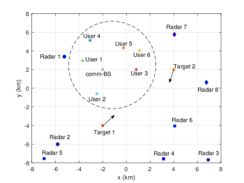
Refer to caption
Figure 5: Test scenario of the HRCN with three types of radars, which coexist with communications BS and users, tracking two moving targets simultaneously.
TABLE II: Initial settings
Radar Type MMR PAR MSR
Index 1 2 3 4 5 6 7 8
Target 1 Initial time (s) 2 2.5 3 2.3 3 3.2 3.2 2.1
revisit interval (s) 2 2 2 3 2 2 2.5 2.5
Target 2 Initial time (s) 2 2.5 3 3 3.5 3.8 4 3.5
revisit interval (s) 2 2 2 3 2 2 2.5 2.5
Refer to caption
Figure 6: Preassigned frequency allocations for the 8 radars, where each block represents the bandwidth ΔfΔ𝑓\Delta f.

V-A ANCHOR performance within a fusion interval

We first explore the performance of ANCHOR within a fusion interval and subsequently consider its performance across intervals.

Convergence and optimized objective function

We assess the performance in the k𝑘k-th fusion interval (i.e. from tksubscript𝑡𝑘t_{k} to tk+1subscript𝑡𝑘1t_{k+1}). Note that the Bayesian CRB matrix 𝑩ksubscript𝑩𝑘\boldsymbol{B}_{k} and the Kalman estimation covariance matrix 𝑪k|ksubscript𝑪conditional𝑘𝑘\boldsymbol{C}_{k|k} should be available as the inputs to the Bayesian tracking scheme in the k𝑘k-th interval. We initialize them with an estimate ( i.e. an amplified version of the state covariance matrix), as is typical in Kalman filtering given that they will converge quickly after the initial phase [58]. Recall that the tracking performance depends on the improvement on the Bayesian CRB, which is evaluated by the objective function q=1Q1Tr(𝚲𝑩1(𝒔tk+1q)𝚲T)superscriptsubscript𝑞1𝑄1Tr𝚲superscript𝑩1superscriptsubscript𝒔subscript𝑡𝑘1𝑞superscript𝚲𝑇\sum_{q=1}^{Q}\frac{1}{\text{Tr}\left(\boldsymbol{\Lambda}\boldsymbol{B}^{-1}\left(\boldsymbol{s}_{t_{k+1}}^{q}\right)\boldsymbol{\Lambda}^{T}\right)}. Therefore, we compare the improvements of the objective value under three resource allocation schemes for the k𝑘k-th fusion interval in Figure 7. For random allocation, we randomly generate the allocated resources satisfying the constraints of problem (26). The uniform allocation distributes the resources equally. The optimized allocation is designed by our proposed algorithm ANCHOR, in which the uniform allocation serves as initialization. Given ANCHOR is based on the alternating optimization method solving two subproblems, we also demonstrate the two nested iterations of the ANCHOR for the first outer iteration. We note that, based on the two nested iterations, the ANCHOR can increase the objective value monotonically as the outer iteration index increases. Compared to the other two allocations, the converged objective value of the optimized allocation is much larger.
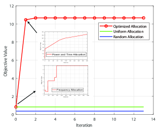
Refer to caption
Figure 7: Comparison of allocation methods in terms of the improvement in the objective value; the insets depict performance improvement with iterations for allocating power-time (top) and frequencies (bottom) for a given outer iteration index.
Radar resource allocation

Fig. 8 demonstrates the allocated radar resources for three methods (random, uniform, and ANCHOR). All values are normalized by the counterparts of the uniform allocation. Note that for the PARs with the optimized allocation, only target 111 is tracked by using radar 555 and 666. In fact, the designed dwell time T4,1,k,T4,2,k,T5,2,ksubscript𝑇41𝑘subscript𝑇42𝑘subscript𝑇52𝑘T_{4,1,k},T_{4,2,k},T_{5,2,k} and T6,2,ksubscript𝑇62𝑘T_{6,2,k} are close to zero numerically, which physically means that the corresponding radars stop scanning at some given time. While it is intuitive that the tracking performance is improved by increasing the power and dwell time as they potentially increase the SINR of the receiving measurements. However, in an interference scenario, we cannot increase all resources while satisfying various constraints and maintaining lower mutual interference. Thus, a trade-off is achieved via the optimized allocation (Fig. 8).
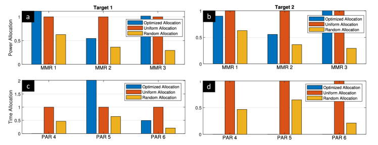
Refer to caption
Figure 8: Power allocation in MIMO radars for (a) Target 1 and (b) Target 2, where all powers under three allocation schemes are normalized by the counterpart of uniform allocation for each radar. Time allocation in phased array radar for (c) target 1 and (d) target 2, where the allocated time is normalized similarly as in uniform allocation.
Communications resource allocation

Fig. 9 shows the power and frequency allocation for the communications downlink transmissions, where the throughput margin is defined as the difference between the achieved and required throughput. Note that the constraint parameters are set to satisfy the uniform allocation in the simulations. Consequently, the throughput margins of the uniform allocation in Fig. 9a are all zero among the users. Interestingly, all users in the random allocation have margins to their throughput thresholds. Compared to the random allocation which only needs to satisfy the constraints of the optimization problem, the ANCHOR allocation optimizes the Bayesian CRB while being feasible to the constraint set. In practice, if the throughput margin is necessary, it is always achieved equivalently by increasing the throughput threshold for the optimized allocation probably at cost of a slight degeneration on tracking performance.
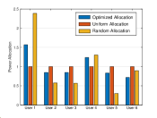
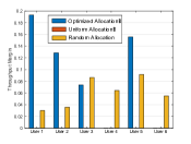
Refer to caption
Refer to caption
(a) Allocation of communications power (left) and throughput margin (the difference between the achieved and required throughput) (right).
Refer to caption
(b) Frequency allocation to communications system.
Figure 9: Resource allocation for communications downlinks.
State estimation performance

For the three allocations, we compare the tracking performance in Table III, where the calibrated root mean square error (CRMSE) is

CRMSE=q=1Q1Nt(n=1Nt𝚲(𝒔~tk+1q(n)𝒔tk+1q)2),CRMSEsuperscriptsubscript𝑞1𝑄1subscript𝑁𝑡superscriptsubscript𝑛1subscript𝑁𝑡superscriptnorm𝚲superscriptsubscript~𝒔subscript𝑡𝑘1𝑞𝑛superscriptsubscript𝒔subscript𝑡𝑘1𝑞2\text{CRMSE}=\sum_{q=1}^{Q}\sqrt{\frac{1}{N_{t}}\left(\sum_{n=1}^{N_{t}}\left\|\boldsymbol{\Lambda}\left(\tilde{\boldsymbol{s}}_{t_{k+1}}^{q\left(n\right)}-\boldsymbol{s}_{t_{k+1}}^{q}\right)\right\|^{2}\right)}, (52)

with Ntsubscript𝑁𝑡N_{t} being the number of the Monte Carlo trials, and the estimated target state is averaged over the Ntsubscript𝑁𝑡N_{t} states. The true target states at time tk+1subscript𝑡𝑘1t_{k+1} are given by 𝒔tk+11=[1.5 km,50 m/s,3.5 km,50 m/s]Tsuperscriptsubscript𝒔subscript𝑡𝑘11superscript1.5 km50 m/s3.5 km50 m/s𝑇\boldsymbol{s}_{t_{k+1}}^{1}=\left[-1.5\text{ km},50\text{ m/s},-3.5\text{ km},50\text{ m/s}\right]^{T} and 𝒔tk+12=[3.75 km,25 m/s,1.5 km,50 m/s]Tsuperscriptsubscript𝒔subscript𝑡𝑘12superscript3.75 km25 m/s1.5 km50 m/s𝑇\boldsymbol{s}_{t_{k+1}}^{2}=\left[3.75\text{ km},-25\text{ m/s},1.5\text{ km},-50\text{ m/s}\right]^{T}. Although the averaged target states are estimated well for all the three allocations, the optimized allocation achieves the smallest CRMSE on average, which reflects the estimation stability over the 500500500 trials.

TABLE III: RMSE and estimated target states over 500 Monte Carlo trials
Allocation CRMSE (m) Target Estimated Target State
Optimized 12.8830 1 [1.5,50,3.5,50]Tsuperscript1.5503.550𝑇\left[-1.5,50,-3.5,50\right]^{T}
2 [3.7497,25.1,1.499,50]Tsuperscript3.749725.11.49950𝑇\left[3.7497,-25.1,1.499,50\right]^{T}
Uniform 87.3946 1 [1.4998,50,3.5001,50]Tsuperscript1.4998503.500150𝑇\left[-1.4998,50,-3.5001,50\right]^{T}
2 [3.75,25,1.5,50]Tsuperscript3.75251.550𝑇\left[-3.75,25,-1.5,50\right]^{T}
Random 113.5374 1 [1.4997,50.1,3.5002,49.9]Tsuperscript1.499750.13.500249.9𝑇\left[-1.4997,50.1,-3.5002,49.9\right]^{T}
2 [3.75,25,1.5001,50]Tsuperscript3.75251.500150𝑇\left[3.75,-25,1.5001,-50\right]^{T}
Performance across scenarios

To explore the statistical stability of the proposed allocation algorithm, we demonstrate the CRMSE performance over 151515 different testing scenarios. In each scenario, the radars are randomly placed to track two targets with randomly generated initial states. The BS is also randomly placed and the communications users are within the BS coverage. The system parameters are initialized correspondingly by the same distributions used in the previous experiments. Fig. 10 shows the CRMSE of a single fusion interval, where the initial 𝑩k|ksubscript𝑩conditional𝑘𝑘\boldsymbol{B}_{k|k} and 𝑪k|ksubscript𝑪conditional𝑘𝑘\boldsymbol{C}_{k|k} are randomly generated for different scenarios. Each CRMSE value is averaged over 200200200 Monte Carlo trials. Clearly, over these scenarios, the average CRMSEs for the optimized allocation are roughly between 100100100 m and 800800800 m, which are further improved in the subsequent fusion intervals.

V-B ANCHOR performance across fusion intervals

We conducted the experiments over 101010 consecutive fusion intervals indexing from k=1𝑘1k=1 to k=10𝑘10k=10. Based on the allocated resources, we update {𝑩k+1q}q=1Qsuperscriptsubscriptsuperscriptsubscript𝑩𝑘1𝑞𝑞1𝑄\left\{\boldsymbol{B}_{k+1}^{q}\right\}_{q=1}^{Q} and {𝑪k+1|k+1}q=1Qsuperscriptsubscriptsubscript𝑪𝑘conditional1𝑘1𝑞1𝑄\left\{\boldsymbol{C}_{k+1|k+1}\right\}_{q=1}^{Q} of the k𝑘k-th fusion interval as the inputs to the next interval. To evaluate the efficacy of the consecutive tracking scheme, we initialized 𝑩1subscript𝑩1\boldsymbol{B}_{1} and 𝑪1|1subscript𝑪conditional11\boldsymbol{C}_{1|1} with a significantly amplified version of the state covariance matrix as a rough guess on the initial state. The tracking estimation is conducted based on (50) and the performance is averaged over 200200200 Monte Carlo trials. The trials are independent and each of them run the 101010 consecutive fusion intervals completely. Fig. 11 demonstrates the averaged values over multiple fusion intervals. Starting with the same values, the optimized allocation improves the objective value significantly compared to the other two allocations. Besides, for the random allocation, it is expected that the objective value fluctuates over the different intervals.
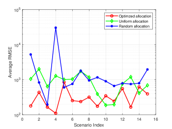
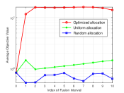
Refer to caption
Figure 10: Average CRMSE of the first fusion interval over 15 different testing scenarios.
Refer to caption
Refer to caption
Figure 11: Average performance over multiple fusion intervals. Left: Average CRB; right: Average CRMSE.
Refer to caption
Refer to caption
Figure 12: Average deviations of target location and velocity.

In terms of the average CRB, the average CRMSE performance over 200 Monte Carlo trials is demonstrated in Fig. 11. The CRMSE values of the three allocations at the first fusion interval is extremely large and close to each other. Recall that we set 𝑩1subscript𝑩1\boldsymbol{B}_{1} and 𝑪1|1subscript𝑪conditional11\boldsymbol{C}_{1|1} with large values to represent a rough initial guess, and thereby we infer that the first tracking performance is heavily influenced by this "bad" initial guess and the improvement brought by the optimized allocation is negligible. Although the first tracking performance is not usable, all three CRMSE curves monotonically decrease with the fusion interval. This validates the efficacy of the Bayesian tracking scheme. The optimized allocation achieves the smallest CRMSE over all fusion intervals.

Fig. 12 shows the tracking performance by inspecting the average deviations of location and velocity over all the intervals. Each average deviation is obtained by calculating the RMSE similar to (52) without matrix 𝚲𝚲\boldsymbol{\varLambda}. Compared to the uniform and random allocations, the optimized allocation consistently performs the best over all fusion intervals for both the location and velocity derivations; this is consistent with the result in Fig. 11 indicating the average CRMSE of the optimized allocation as being the lowest. In addition, it is interesting to note that the velocity derivation has a relatively large fluctuation at the second fusion interval compared to the monotonicity of the location derivation. To explain this phenomenon, recall that each radar can only observe the radial velocity in our system model and thereby an accurate estimation on target velocity relies on the information fusion from all radars. Each radar is expected to provide some “unique” information about the velocity, which requires a proper placement of the radars with respect to the tracking target. Otherwise, the velocity ambiguity cannot be reduced substantially and consequently leads to unsatisfying velocity estimation.

VI Summary

We considered spectrum sharing between heterogeneously-distributed JRC with the goal of tracking multiple radar targets while maintaining the throughput levels for the communications downlinks. Within the asynchronous multi-target tracking framework, we proposed a Bayesian CRB-based metric for optimization, which further depends on the system resources (i.e. radar and communications power, dwell time, and shared bandwidth). The resulting resource allocation problem was non-convex and involved discrete and continuous variables. We solved this through our proposed ANCHOR algorithm based on the alternating optimization framework with guaranteed monotonicity. The frequency and power-time were allocated alternately. Our numerical experiments illustrated the key algorithmic and system aspects of resource allocation. We demonstrated that, compared to the trivial uniform and random allocations, the system performance is significantly improved by properly allocating the accessible heterogeneous resources of both radar and communications through ANCHOR algorithm. This study is helpful in meeting challenges of next-generation wireless systems where heterogeneous networks are envisaged such as different radio access technologies (RATs) and cell-free massive MIMO systems [59].

-A Proof of Lemma 1

By definition, the FIM 𝑱𝒚kq(𝒔tk+1q)subscript𝑱superscriptsubscript𝒚𝑘𝑞superscriptsubscript𝒔subscript𝑡𝑘1𝑞\boldsymbol{J}_{\boldsymbol{y}_{k}^{q}}\left(\boldsymbol{s}_{t_{k+1}}^{q}\right) is 𝑱𝒚kq(𝒔tk+1q)=𝔼{[𝒔tk+1qlnp(𝒚kq|𝒔tk+1q)][𝒔tk+1qlnp(𝒚kq|𝒔tk+1q)]T}subscript𝑱superscriptsubscript𝒚𝑘𝑞superscriptsubscript𝒔subscript𝑡𝑘1𝑞𝔼delimited-[]subscriptsuperscriptsubscript𝒔subscript𝑡𝑘1𝑞𝑝conditionalsuperscriptsubscript𝒚𝑘𝑞superscriptsubscript𝒔subscript𝑡𝑘1𝑞superscriptdelimited-[]subscriptsuperscriptsubscript𝒔subscript𝑡𝑘1𝑞𝑝conditionalsuperscriptsubscript𝒚𝑘𝑞superscriptsubscript𝒔subscript𝑡𝑘1𝑞𝑇\boldsymbol{J}_{\boldsymbol{y}_{k}^{q}}\left(\boldsymbol{s}_{t_{k+1}}^{q}\right)=\mathbb{E}\left\{\left[\nabla_{\boldsymbol{s}_{t_{k+1}}^{q}}\ln p\left(\boldsymbol{y}_{k}^{q}|\boldsymbol{s}_{t_{k+1}}^{q}\right)\right]\left[\nabla_{\boldsymbol{s}_{t_{k+1}}^{q}}\ln p\left(\boldsymbol{y}_{k}^{q}|\boldsymbol{s}_{t_{k+1}}^{q}\right)\right]^{T}\right\}. Since the measurement 𝒚kqsuperscriptsubscript𝒚𝑘𝑞\boldsymbol{y}_{k}^{q} follows a normal distribution with p(𝒚kq|𝒔tk+1q)=i=1NmMi,q,k𝒩(h(𝒔i,q,km,i),𝚺i,q,km)𝑝conditionalsuperscriptsubscript𝒚𝑘𝑞superscriptsubscript𝒔subscript𝑡𝑘1𝑞superscriptsubscriptproduct𝑖1𝑁superscriptsubscriptproduct𝑚subscript𝑀𝑖𝑞𝑘𝒩superscriptsubscript𝒔𝑖𝑞𝑘𝑚𝑖superscriptsubscript𝚺𝑖𝑞𝑘𝑚p\left(\boldsymbol{y}_{k}^{q}|\boldsymbol{s}_{t_{k+1}}^{q}\right)=\prod_{i=1}^{N}\prod_{m}^{M_{i,q,k}}\mathcal{N}\left(h\left(\boldsymbol{s}_{i,q,k}^{m},i\right),\boldsymbol{\Sigma}_{i,q,k}^{m}\right), we have

𝒔tk+1qlnp(𝒚kq|𝒔tk+1q)subscriptsuperscriptsubscript𝒔subscript𝑡𝑘1𝑞𝑝conditionalsuperscriptsubscript𝒚𝑘𝑞superscriptsubscript𝒔subscript𝑡𝑘1𝑞\displaystyle\nabla_{\boldsymbol{s}_{t_{k+1}}^{q}}\ln p\left(\boldsymbol{y}_{k}^{q}|\boldsymbol{s}_{t_{k+1}}^{q}\right) (53)
=\displaystyle= i=1Nm=1Mi,q,k𝑯i,q,kmT(𝚺i,q,km)1(𝒚kqh(𝒔i,q,km,i)),superscriptsubscript𝑖1𝑁superscriptsubscript𝑚1subscript𝑀𝑖𝑞𝑘superscriptsubscript𝑯𝑖𝑞𝑘𝑚𝑇superscriptsuperscriptsubscript𝚺𝑖𝑞𝑘𝑚1superscriptsubscript𝒚𝑘𝑞superscriptsubscript𝒔𝑖𝑞𝑘𝑚𝑖\displaystyle\sum_{i=1}^{N}\sum_{m=1}^{M_{i,q,k}}\boldsymbol{H}_{i,q,k}^{mT}\left(\boldsymbol{\Sigma}_{i,q,k}^{m}\right)^{-1}\left(\boldsymbol{y}_{k}^{q}-h\left(\boldsymbol{s}_{i,q,k}^{m},i\right)\right),

where 𝑯i,q,kmsuperscriptsubscript𝑯𝑖𝑞𝑘𝑚\boldsymbol{H}_{i,q,k}^{m} is the Jacobian matrix of h(𝒔i,q,km,i)superscriptsubscript𝒔𝑖𝑞𝑘𝑚𝑖h\left(\boldsymbol{s}_{i,q,k}^{m},i\right) on 𝒔tk+1qsuperscriptsubscript𝒔subscript𝑡𝑘1𝑞\boldsymbol{s}_{t_{k+1}}^{q} based on 𝒔tk+1q=f(𝒔i,q,km,tk+1ti,q,km)superscriptsubscript𝒔subscript𝑡𝑘1𝑞𝑓superscriptsubscript𝒔𝑖𝑞𝑘𝑚subscript𝑡𝑘1superscriptsubscript𝑡𝑖𝑞𝑘𝑚\boldsymbol{s}_{t_{k+1}}^{q}=f\left(\boldsymbol{s}_{i,q,k}^{m},t_{k+1}-t_{i,q,k}^{m}\right).

We have

𝔼[(𝒚kqh(𝒔i,q,km,i))(𝒚kqh(𝒔i,q,km,i))T]𝔼delimited-[]superscriptsubscript𝒚𝑘𝑞superscriptsubscript𝒔𝑖𝑞𝑘𝑚𝑖superscriptsuperscriptsubscript𝒚𝑘𝑞superscriptsubscript𝒔superscript𝑖superscript𝑞𝑘𝑚𝑖𝑇\displaystyle\mathbb{E}\left[\left(\boldsymbol{y}_{k}^{q}-h\left(\boldsymbol{s}_{i,q,k}^{m},i\right)\right)\left(\boldsymbol{y}_{k}^{q}-h\left(\boldsymbol{s}_{i^{\prime},q^{\prime},k}^{m},i\right)\right)^{T}\right] (54)
=\displaystyle= {𝚺i,q,kmi=i,p=p𝟎otherwise.casessuperscriptsubscript𝚺𝑖𝑞𝑘𝑚formulae-sequence𝑖superscript𝑖𝑝superscript𝑝0otherwise\displaystyle\begin{cases}\boldsymbol{\Sigma}_{i,q,k}^{m}&i=i^{\prime},p=p^{\prime}\\ \boldsymbol{0}&\text{otherwise}.\end{cases}

Hence, substituting (53) into 𝑱𝒚kqsubscript𝑱superscriptsubscript𝒚𝑘𝑞\boldsymbol{J}_{\boldsymbol{y}_{k}^{q}} yields 𝑱𝒚kq(𝒔tk+1q)=i=1NmMi,q,kPi,q,kmTi,q,kmj=1Jαi,jcPc,kj+σr,i2𝑯i,q,kmT(𝑪i,q,km)1𝑯i,q,kmsubscript𝑱superscriptsubscript𝒚𝑘𝑞superscriptsubscript𝒔subscript𝑡𝑘1𝑞superscriptsubscript𝑖1𝑁superscriptsubscript𝑚subscript𝑀𝑖𝑞𝑘superscriptsubscript𝑃𝑖𝑞𝑘𝑚superscriptsubscript𝑇𝑖𝑞𝑘𝑚superscriptsubscript𝑗1𝐽superscriptsubscript𝛼𝑖𝑗𝑐superscriptsubscript𝑃𝑐𝑘𝑗superscriptsubscript𝜎𝑟𝑖2superscriptsubscript𝑯𝑖𝑞𝑘𝑚𝑇superscriptsuperscriptsubscript𝑪𝑖𝑞𝑘𝑚1superscriptsubscript𝑯𝑖𝑞𝑘𝑚\boldsymbol{J}_{\boldsymbol{y}_{k}^{q}}\left(\boldsymbol{s}_{t_{k+1}}^{q}\right)=\sum_{i=1}^{N}\sum_{m}^{M_{i,q,k}}\frac{P_{i,q,k}^{m}T_{i,q,k}^{m}}{\sum_{j=1}^{J}\alpha_{i,j}^{c}P_{c,k}^{j}+\sigma_{r,i}^{2}}\boldsymbol{H}_{i,q,k}^{mT}\left(\boldsymbol{C}_{i,q,k}^{m}\right)^{-1}\boldsymbol{H}_{i,q,k}^{m}. This completes the proof.

-B Proof of Lemma 2

The inner minimization problem w.r.t. {𝑽q}subscript𝑽𝑞\left\{\boldsymbol{V}_{q}\right\} is

minimize{𝑽q}subscript𝑽𝑞minimize\displaystyle\underset{\left\{\boldsymbol{V}_{q}\right\}}{\text{minimize}} q=1QTr(𝑽qT𝚲~T𝑩q𝚲~𝑽q)superscriptsubscript𝑞1𝑄Trsuperscriptsubscript𝑽𝑞𝑇superscript~𝚲𝑇subscript𝑩𝑞~𝚲subscript𝑽𝑞\displaystyle\sum_{q=1}^{Q}\text{Tr}\left(\boldsymbol{V}_{q}^{T}\tilde{\boldsymbol{\Lambda}}^{T}\boldsymbol{B}_{q}\tilde{\boldsymbol{\Lambda}}\boldsymbol{V}_{q}\right) (55)
subject to Tr(𝑽q)=1,q=1,Q,formulae-sequenceTrsubscript𝑽𝑞1for-all𝑞1𝑄\displaystyle\text{Tr}\left(\boldsymbol{V}_{q}\right)=1,\forall q=1,\ldots Q,

which is further decoupled into Q𝑄Q subproblems as

minimize𝑽qsubscript𝑽𝑞minimize\displaystyle\underset{\boldsymbol{V}_{q}}{\text{minimize}} Tr(𝑽qT𝚲~T𝑩q𝚲~𝑽q)Trsuperscriptsubscript𝑽𝑞𝑇superscript~𝚲𝑇subscript𝑩𝑞~𝚲subscript𝑽𝑞\displaystyle\text{Tr}\left(\boldsymbol{V}_{q}^{T}\tilde{\boldsymbol{\Lambda}}^{T}\boldsymbol{B}_{q}\tilde{\boldsymbol{\Lambda}}\boldsymbol{V}_{q}\right) (56)
subject to Tr(𝑽q)=1.Trsubscript𝑽𝑞1\displaystyle\text{Tr}\left(\boldsymbol{V}_{q}\right)=1.

Problem (56) has the Lagrangian (𝑽q,λq)=Tr(𝑽qT𝚲~T𝑩q𝚲~𝑽q)+λq(Tr(𝑽q)1)subscript𝑽𝑞subscript𝜆𝑞Trsuperscriptsubscript𝑽𝑞𝑇superscript~𝚲𝑇subscript𝑩𝑞~𝚲subscript𝑽𝑞subscript𝜆𝑞Trsubscript𝑽𝑞1\mathcal{L}\left(\boldsymbol{V}_{q},\lambda_{q}\right)=\text{Tr}\left(\boldsymbol{V}_{q}^{T}\tilde{\boldsymbol{\Lambda}}^{T}\boldsymbol{B}_{q}\tilde{\boldsymbol{\Lambda}}\boldsymbol{V}_{q}\right)+\lambda_{q}\left(\text{Tr}\left(\boldsymbol{V}_{q}\right)-1\right). Following the Lagrangian method yields

{𝑽q=2𝚲~T𝑩q𝚲~𝑽q+λq𝑰=0λq=Tr(𝑽q)1=0,casessuperscript𝑽𝑞2superscript~𝚲𝑇subscript𝑩𝑞~𝚲subscript𝑽𝑞subscript𝜆𝑞𝑰0otherwisesubscript𝜆𝑞Trsubscript𝑽𝑞10otherwise\begin{cases}\frac{\partial\mathcal{L}}{\partial\boldsymbol{V}^{q}}=2\tilde{\boldsymbol{\Lambda}}^{T}\boldsymbol{B}_{q}\tilde{\boldsymbol{\Lambda}}\boldsymbol{V}_{q}+\lambda_{q}\boldsymbol{I}=0\\ \frac{\partial\mathcal{L}}{\partial\lambda_{q}}=\text{Tr}\left(\boldsymbol{V}_{q}\right)-1=0,\end{cases} (57)

which has the solution

{𝑽q=(𝚲~T𝑩q𝚲~)1Tr[(𝚲~T𝑩q𝚲~)1]𝟎λq=2Tr[(𝚲~T𝑩q𝚲~)1].casessuperscriptsubscript𝑽𝑞superscriptsuperscript~𝚲𝑇subscript𝑩𝑞~𝚲1Trdelimited-[]superscriptsuperscript~𝚲𝑇subscript𝑩𝑞~𝚲1succeeds-or-equals0otherwisesuperscriptsubscript𝜆𝑞2Trdelimited-[]superscriptsuperscript~𝚲𝑇subscript𝑩𝑞~𝚲1otherwise\begin{cases}\boldsymbol{V}_{q}^{\star}=\frac{\left(\tilde{\boldsymbol{\Lambda}}^{T}\boldsymbol{B}_{q}\tilde{\boldsymbol{\Lambda}}\right)^{-1}}{\text{Tr}\left[\left(\tilde{\boldsymbol{\Lambda}}^{T}\boldsymbol{B}_{q}\tilde{\boldsymbol{\Lambda}}\right)^{-1}\right]}\succeq\boldsymbol{0}\\ \lambda_{q}^{\star}=\frac{-2}{\text{Tr}\left[\left(\tilde{\boldsymbol{\Lambda}}^{T}\boldsymbol{B}_{q}\tilde{\boldsymbol{\Lambda}}\right)^{-1}\right]}.\end{cases} (58)

Substituting the expression of 𝑽qsuperscriptsubscript𝑽𝑞\boldsymbol{V}_{q}^{\star} into the objective function of problem (33), we have

q=1QTr((𝑽q)T𝚲~T𝑩q𝚲~𝑽q)=q=1Q1Tr(𝚲𝑩q1𝚲T),superscriptsubscript𝑞1𝑄Trsuperscriptsuperscriptsubscript𝑽𝑞𝑇superscript~𝚲𝑇subscript𝑩𝑞~𝚲superscriptsubscript𝑽𝑞superscriptsubscript𝑞1𝑄1Tr𝚲superscriptsubscript𝑩𝑞1superscript𝚲𝑇\sum_{q=1}^{Q}\text{Tr}\left(\left(\boldsymbol{V}_{q}^{\star}\right)^{T}\tilde{\boldsymbol{\Lambda}}^{T}\boldsymbol{B}_{q}\tilde{\boldsymbol{\Lambda}}\boldsymbol{V}_{q}^{\star}\right)=\sum_{q=1}^{Q}\frac{1}{\text{Tr}\left(\boldsymbol{\Lambda}\boldsymbol{B}_{q}^{-1}\boldsymbol{\Lambda}^{T}\right)}, (59)

which is the objective function of problem (26). This completes the proof.

-C Proof of Lemma 3

Define w(𝒛,𝑽q)=Tr(𝑽qT𝚲~T𝑩q𝚲~𝑽q)𝑤𝒛subscript𝑽𝑞Trsuperscriptsubscript𝑽𝑞𝑇superscript~𝚲𝑇subscript𝑩𝑞~𝚲subscript𝑽𝑞w\left(\boldsymbol{z},\boldsymbol{V}_{q}\right)=\text{Tr}\left(\boldsymbol{V}_{q}^{T}\tilde{\boldsymbol{\Lambda}}^{T}\boldsymbol{B}_{q}\tilde{\boldsymbol{\Lambda}}\boldsymbol{V}_{q}\right) and w~(𝒛)=min{𝑽q}q=1Qw(𝒛,𝑽q)~𝑤𝒛subscript𝑽𝑞superscriptsubscript𝑞1𝑄𝑤𝒛subscript𝑽𝑞\tilde{w}\left(\boldsymbol{z}\right)=\underset{\left\{\boldsymbol{V}_{q}\right\}}{\min}\sum_{q=1}^{Q}w\left(\boldsymbol{z},\boldsymbol{V}_{q}\right), which is the objective function of problem (33). The function w(𝒛,{𝑽q})𝑤𝒛subscript𝑽𝑞w\left(\boldsymbol{z},\left\{\boldsymbol{V}_{q}\right\}\right) is differentiable in 𝒛𝒛\boldsymbol{z} and the feasible set 𝒵𝒵\mathcal{Z} is convex. Furthermore, w(𝒛,𝑽q)𝑤𝒛subscript𝑽𝑞w\left(\boldsymbol{z},\boldsymbol{V}_{q}\right) is strongly convex in 𝑽qsubscript𝑽𝑞\boldsymbol{V}_{q} and the set 𝒱q={𝑽q|Tr(𝑽q)=1,𝑽q𝟎}subscript𝒱𝑞conditional-setsubscript𝑽𝑞formulae-sequenceTrsubscript𝑽𝑞1succeeds-or-equalssubscript𝑽𝑞0\mathcal{V}_{q}=\left\{\boldsymbol{V}_{q}|\text{Tr}\left(\boldsymbol{V}_{q}\right)=1,\boldsymbol{V}_{q}\succeq\boldsymbol{0}\right\} is compact. Thus, by applying the Danskin’s theorem [60], we have w~(𝒛)=q=1Q𝑽qw(𝒛,𝑽q)|𝑽q=𝑽q~𝑤𝒛evaluated-atsuperscriptsubscript𝑞1𝑄subscriptsubscript𝑽𝑞𝑤𝒛subscript𝑽𝑞subscript𝑽𝑞superscriptsubscript𝑽𝑞\nabla\tilde{w}\left(\boldsymbol{z}\right)=\sum_{q=1}^{Q}\partial_{\boldsymbol{V}_{q}}w\left(\boldsymbol{z},\boldsymbol{V}_{q}\right)|_{\boldsymbol{V}_{q}=\boldsymbol{V}_{q}^{\star}}, where 𝑽q=argminTr(𝑽q)=1,𝑽q𝟎{Tr(𝑽qT𝚲~T𝑩q𝚲~𝑽q)}superscriptsubscript𝑽𝑞formulae-sequenceTrsubscript𝑽𝑞1succeeds-or-equalssubscript𝑽𝑞0minTrsuperscriptsubscript𝑽𝑞𝑇superscript~𝚲𝑇subscript𝑩𝑞~𝚲subscript𝑽𝑞\boldsymbol{V}_{q}^{\star}=\arg\underset{\text{Tr}\left(\boldsymbol{V}_{q}\right)=1,\boldsymbol{V}_{q}\succeq\boldsymbol{0}}{\text{min}}\left\{\text{Tr}\left(\boldsymbol{V}_{q}^{T}\tilde{\boldsymbol{\Lambda}}^{T}\boldsymbol{B}_{q}\tilde{\boldsymbol{\Lambda}}\boldsymbol{V}_{q}\right)\right\}. From this perspective, the update rules of Algorithm 3 can be merged into 𝒛n+1=𝒫𝒵(𝒛nηw~(𝒛n))superscript𝒛𝑛1subscript𝒫𝒵superscript𝒛𝑛𝜂~𝑤superscript𝒛𝑛\boldsymbol{z}^{n+1}=\mathcal{P}_{\mathcal{Z}}\left(\boldsymbol{z}^{n}-\eta\nabla\tilde{w}\left(\boldsymbol{z}^{n}\right)\right). By applying [61, Theorem 31] with ϵ=0italic-ϵ0\epsilon=0 (due to the availability of the optimal 𝑽𝑽\boldsymbol{V}), we arrive at the conclusion that the sequence {𝒛n}superscript𝒛𝑛\left\{\boldsymbol{z}^{n}\right\} will converge to the stationary point of w~(𝒛)~𝑤𝒛\tilde{w}\left(\boldsymbol{z}\right) for 𝒛𝒵𝒛𝒵\boldsymbol{z}\in\mathcal{Z}.

-D Proof of Theorem 4

At the \ell-th iteration, the objective value of problem (26) is g(𝒛,𝑭c)𝑔subscript𝒛superscriptsubscript𝑭𝑐g\left(\boldsymbol{z}_{\ell},\boldsymbol{F}_{\ell}^{c}\right). We have g(𝒛,𝑭c)g(𝒛,𝑭+1c)g(𝒛+1,𝑭+1c)𝑔subscript𝒛superscriptsubscript𝑭𝑐𝑔subscript𝒛superscriptsubscript𝑭1𝑐𝑔subscript𝒛1superscriptsubscript𝑭1𝑐g\left(\boldsymbol{z}_{\ell},\boldsymbol{F}_{\ell}^{c}\right)\leq g\left(\boldsymbol{z}_{\ell},\boldsymbol{F}_{\ell+1}^{c}\right)\leq g\left(\boldsymbol{z}_{\ell+1},\boldsymbol{F}_{\ell+1}^{c}\right), where the first inequality holds because of Algorithm 2, and the second inequality holds because Algorithm 3 converges to a stationary point. Thus, the sequence {g(𝒛,𝑭c)}𝑔subscript𝒛superscriptsubscript𝑭𝑐\left\{g\left(\boldsymbol{z}_{\ell},\boldsymbol{F}_{\ell}^{c}\right)\right\} is non-decreasing. Since the objective function g(𝒛,𝑭c)𝑔𝒛superscript𝑭𝑐g\left(\boldsymbol{z},\boldsymbol{F}^{c}\right) is upper-bounded, the non-decreasing {g(𝒛,𝑭c)}𝑔subscript𝒛superscriptsubscript𝑭𝑐\left\{g\left(\boldsymbol{z}_{\ell},\boldsymbol{F}_{\ell}^{c}\right)\right\} will converge to a finite value.

References

  • [1] K. V. Mishra, M. R. Bhavani Shankar, V. Koivunen, B. Ottersten, and S. A. Vorobyov, “Toward millimeter wave joint radar-communications: A signal processing perspective,” IEEE Signal Processing Magazine, vol. 36, no. 5, pp. 100–114, 2019.
  • [2] F. Liu, C. Masouros, A. P. Petropulu, H. Griffiths, and L. Hanzo, “Joint radar and communication design: Applications, state-of-the-art, and the road ahead,” IEEE Transactions on Communications, vol. 68, no. 6, pp. 3834–3862, 2020.
  • [3] M. I. Skolnik, Radar handbook, 3rd ed.   McGraw-Hill, 2008.
  • [4] J. G. Proakis and M. Salehi, Digital Communications, 5th ed.   New York, NY: McGraw-Hill, 2008.
  • [5] Z. Khan, J. J. Lehtomaki, R. Vuohtoniemi, E. Hossain, and L. A. DaSilva, “On opportunistic spectrum access in radar bands: Lessons learned from measurement of weather radar signals,” IEEE Wireless Communications, vol. 23, no. 3, pp. 40–48, 2016.
  • [6] Y. Cui, V. Koivunen, and X. Jing, “Interference alignment based spectrum sharing for MIMO radar and communication systems,” in IEEE International Workshop on Signal Processing Advances in Wireless Communications, 2018, pp. 1–5.
  • [7] A. Ayyar and K. V. Mishra, “Robust communications-centric coexistence for turbo-coded OFDM with non-traditional radar interference models,” in IEEE Radar Conference, 2019, pp. 1–6.
  • [8] L. Wu and D. P. Palomar, “Sequence design for spectral shaping via minimization of regularized spectral level ratio,” IEEE Transactions on Signal Processing, vol. 67, no. 18, pp. 4683–4695, 2019.
  • [9] S. H. Dokhanchi, B. S. Mysore, K. V. Mishra, and B. Ottersten, “A mmWave automotive joint radar-communications system,” IEEE Transactions on Aerospace and Electronic Systems, vol. 55, no. 3, pp. 1241–1260, 2019.
  • [10] F. Liu, L. Zhou, C. Masouros, A. Li, W. Luo, and A. Petropulu, “Toward dual-functional radar-communication systems: Optimal waveform design,” IEEE Transactions on Signal Processing, vol. 66, no. 16, pp. 4264–4279, 2018.
  • [11] F. Liu, Y. Cui, C. Masouros, J. Xu, T. X. Han, Y. C. Eldar, and S. Buzzi, “Integrated sensing and communications: Towards dual-functional wireless networks for 6G and beyond,” 2021.
  • [12] H. Shajaiah, A. Khawar, A. Abdel-Hadi, and T. C. Clancy, “Resource allocation with carrier aggregation in LTE advanced cellular system sharing spectrum with S-band radar,” in IEEE International Symposium on Dynamic Spectrum Access Networks, 2014, pp. 34–37.
  • [13] P. S. Tan, J. M. Stiles, and S. D. Blunt, “Optimizing sparse allocation for radar spectrum sharing,” in IEEE Radar Conference, 2016, pp. 1–6.
  • [14] M. Scharrenbroich and M. Zatman, “Joint radar-communications resource management,” in IEEE Radar Conference, 2016, pp. 1–6.
  • [15] B. Li and A. P. Petropulu, “Joint transmit designs for coexistence of mimo wireless communications and sparse sensing radars in clutter,” IEEE Transactions on Aerospace and Electronic Systems, vol. 53, no. 6, pp. 2846–2864, 2017.
  • [16] A. Hassanien, M. G. Amin, E. Aboutanios, and B. Himed, “Dual-function radar communication systems: A solution to the spectrum congestion problem,” IEEE Signal Processing Magazine, vol. 36, no. 5, pp. 115–126, 2019.
  • [17] A. M. Elbir, K. V. Mishra, and S. Chatzinotas, “Terahertz-band joint ultra-massive MIMO radar-communications: Model-based and model-free hybrid beamforming,” IEEE Journal of Selected Topics in Signal Processing, vol. 15, no. 6, pp. 1468–1483, 2021.
  • [18] Q. He, Z. Wang, J. Hu, and R. S. Blum, “Performance gains from cooperative MIMO radar and MIMO communication systems,” IEEE Signal Processing Letters, vol. 26, no. 1, pp. 194–198, 2019.
  • [19] S. Sun, K. V. Mishra, and A. P. Petropulu, “Target estimation by exploiting low rank structure in widely separated MIMO radar,” in IEEE Radar Conference, 2019, pp. 1–6.
  • [20] S. Sedighi, K. V. Mishra, M. B. Shankar, and B. Ottersten, “Localization with one-bit passive radars in narrowband internet-of-things using multivariate polynomial optimization,” IEEE Transactions on Signal Processing, vol. 69, pp. 2525–2540, 2021.
  • [21] J. Liu, K. V. Mishra, and M. Saquib, “Co-designing statistical MIMO radar and in-band full-duplex multi-user MIMO communications,” arXiv preprint arXiv:2006.14774, 2020.
  • [22] G. Wang and K. V. Mishra, “Displaced sensor automotive radar imaging,” arXiv preprint arXiv:2010.04085, 2020.
  • [23] A. Ahmed, Y. D. Zhang, and B. Himed, “Distributed dual-function radar-communication MIMO system with optimized resource allocation,” in IEEE Radar Conference, 2019, pp. 1–5.
  • [24] J. Yan, H. Liu, W. Pu, S. Zhou, Z. Liu, and Z. Bao, “Joint beam selection and power allocation for multiple target tracking in netted colocated mimo radar system,” IEEE Transactions on Signal Processing, vol. 64, no. 24, pp. 6417–6427, 2016.
  • [25] J. Yan, W. Pu, H. Liu, S. Zhou, and Z. Bao, “Cooperative target assignment and dwell allocation for multiple target tracking in phased array radar network,” Signal Processing, vol. 141, pp. 74–83, 2017.
  • [26] J. Yan, H. Liu, W. Pu, H. Liu, Z. Liu, and Z. Bao, “Joint threshold adjustment and power allocation for cognitive target tracking in asynchronous radar network,” IEEE Transactions on Signal Processing, vol. 65, no. 12, pp. 3094–3106, 2017.
  • [27] J. Yan, W. Pu, S. Zhou, H. Liu, and M. S. Greco, “Optimal resource allocation for asynchronous multiple targets tracking in heterogeneous radar networks,” IEEE Transactions on Signal Processing, vol. 68, pp. 4055–4068, 2020.
  • [28] J. Yan, J. Dai, W. Pu, H. Liu, and M. Greco, “Target capacity based resource optimization for multiple target tracking in radar network,” IEEE Transactions on Signal Processing, vol. 69, pp. 2410–2421, 2021.
  • [29] S. Karimi-Bidhendi, J. Guo, and H. Jafarkhani, “Energy-efficient node deployment in heterogeneous two-tier wireless sensor networks with limited communication range,” IEEE Transactions on Wireless Communications, vol. 20, no. 1, pp. 40–55, 2021.
  • [30] ——, “Energy-efficient node deployment in static and mobile heterogeneous multi-hop wireless sensor networks,” IEEE Transactions on Wireless Communications, 2022, in press.
  • [31] L. Wu, K. V. Mishra, M. R. B. Shankar, B. Ottersten et al., “Heterogeneously-distributed joint radar communications: Bayesian resource allocation,” in IEEE International Workshop on Signal Processing Advances in Wireless Communications, 2021, pp. 506–510.
  • [32] R. Olfati-Saber and J. S. Shamma, “Consensus filters for sensor networks and distributed sensor fusion,” in IEEE Conference on Decision and Control, 2005, pp. 6698–6703.
  • [33] H. Chen, T. Kirubarajan, and Y. Bar-Shalom, “Performance limits of track-to-track fusion versus centralized estimation: Theory and application,” IEEE Transactions on Aerospace and Electronic Systems, vol. 39, no. 2, pp. 386–400, 2003.
  • [34] T. O. Olwal, K. Djouani, and A. M. Kurien, “A survey of resource management toward 5G radio access networks,” IEEE Communications Surveys & Tutorials, vol. 18, no. 3, pp. 1656–1686, 2016.
  • [35] M. Hasan and E. Hossain, “Distributed resource allocation in D2D-enabled multi-tier cellular networks: An auction approach,” in IEEE international conference on communications, 2015, pp. 2949–2954.
  • [36] B. D. Cordill, S. A. Seguin, and L. Cohen, “Electromagnetic interference to radar receivers due to in-band OFDM communications systems,” in IEEE International Symposium on Electromagnetic Compatibility, 2013, pp. 72–75.
  • [37] J. Rodriguez-Fernandez and N. Gonzalez-Prelcic, “Channel estimation for frequency-selective mmWave MIMO systems with beam-squint,” in IEEE Global Communications Conference, 2018, pp. 1–6.
  • [38] M. I. Skolnik, “Theoretical accuracy of radar measurements,” IRE Transactions on Aeronautical and Navigational Electronics, vol. ANE-7, no. 4, pp. 123–129, 1960.
  • [39] P. Z. Peebles, Radar principles.   John Wiley & Sons, 2007.
  • [40] I. Klein and Y. Bar-Shalom, “Tracking with asynchronous passive multisensor systems,” IEEE Transactions on Aerospace and Electronic Systems, vol. 52, no. 4, pp. 1769–1776, 2016.
  • [41] R. W. Osborne and Y. Bar-Shalom, “Statistical efficiency of composite position measurements from passive sensors,” IEEE Transactions on Aerospace and Electronic Systems, vol. 49, no. 4, pp. 2799–2806, 2013.
  • [42] Y. Bar-Shalom, X. R. Li, and T. Kirubarajan, Estimation with applications to tracking and navigation: Theory algorithms and software.   John Wiley & Sons, 2004.
  • [43] J. Yan, B. Jiu, H. Liu, B. Chen, and Z. Bao, “Prior knowledge-based simultaneous multibeam power allocation algorithm for cognitive multiple targets tracking in clutter,” IEEE Transactions on Signal Processing, vol. 63, no. 2, pp. 512–527, 2014.
  • [44] H. W. Kuhn, “The Hungarian method for the assignment problem,” Naval Research Logistics Quarterly, vol. 2, no. 1-2, pp. 83–97, 1955.
  • [45] P. M. Pardalos and L. S. Pitsoulis, Nonlinear assignment problems: Algorithms and applications.   Springer Science & Business Media, 2013, vol. 7.
  • [46] D. Henderson, S. H. Jacobson, and A. W. Johnson, “The theory and practice of simulated annealing,” in Handbook of Metaheuristics.   Springer, 2003, pp. 287–319.
  • [47] M. Nouiehed, M. Sanjabi, T. Huang, J. D. Lee, and M. Razaviyayn, “Solving a class of non-convex min-max games using iterative first order methods,” Advances in Neural Information Processing Systems 32, p. 14905–14916, 2019.
  • [48] S. Lu, I. Tsaknakis, M. Hong, and Y. Chen, “Hybrid block successive approximation for one-sided non-convex min-max problems: algorithms and applications,” IEEE Transactions on Signal Processing, vol. 68, pp. 3676–3691, 2020.
  • [49] M. Razaviyayn, M. Hong, and Z.-Q. Luo, “A unified convergence analysis of block successive minimization methods for nonsmooth optimization,” SIAM Journal on Optimization, vol. 23, no. 2, pp. 1126–1153, 2013.
  • [50] M. Razaviyayn, T. Huang, S. Lu, M. Nouiehed, M. Sanjabi, and M. Hong, “Nonconvex min-max optimization: Applications, challenges, and recent theoretical advances,” IEEE Signal Processing Magazine, vol. 37, no. 5, pp. 55–66, 2020.
  • [51] H. Benson, “On the global optimization of sums of linear fractional functions over a convex set,” Journal of Optimization Theory and Applications, vol. 121, no. 1, pp. 19–39, 2004.
  • [52] J. E. Falk and S. W. Palocsay, “Optimizing the sum of linear fractional functions,” in Recent Advances in Global Optimization.   Princeton University Press, 2014, pp. 221–258.
  • [53] N. T. H. Phuong and H. Tuy, “A unified monotonic approach to generalized linear fractional programming,” Journal of Global Optimization, vol. 26, no. 3, pp. 229–259, 2003.
  • [54] K. Shen and W. Yu, “Fractional programming for communication systems—Part I: Power control and beamforming,” IEEE Transactions on Signal Processing, vol. 66, no. 10, pp. 2616–2630, 2018.
  • [55] A. Meijerink and A. F. Molisch, “On the physical interpretation of the Saleh–Valenzuela model and the definition of its power delay profiles,” IEEE Transactions on Antennas and Propagation, vol. 62, no. 9, pp. 4780–4793, 2014.
  • [56] C. Gustafson, K. Haneda, S. Wyne, and F. Tufvesson, “On mm-wave multipath clustering and channel modeling,” IEEE Transactions on Antennas and Propagation, vol. 62, no. 3, pp. 1445–1455, 2013.
  • [57] H. Zhang, S. Venkateswaran, and U. Madhow, “Channel modeling and MIMO capacity for outdoor millimeter wave links,” in IEEE Wireless Communication and Networking Conference, 2010, pp. 1–6.
  • [58] R. E. Kalman, “A new approach to linear filtering and prediction problems,” Journal of Basic Engineering, vol. 82-D, no. 4, pp. 35–45, 1960.
  • [59] A. Flores, R. C. de Lamare, and K. V. Mishra, “Rate-splitting meets cell-free MIMO communications,” arXiv preprint arXiv:2112.00884, 2021.
  • [60] J. M. Danskin, The theory of max-min and its application to weapons allocation problems.   Springer Science & Business Media, 2012, vol. 5.
  • [61] C. Jin, P. Netrapalli, and M. Jordan, “What is local optimality in nonconvex-nonconcave minimax optimization?” in International Conference on Machine Learning, 2020, pp. 4880–4889.
[Uncaptioned image] Linlong Wu received the B.E. degree in electronic information from Xi’an Jiaotong University (XJTU), Xi’an, China, in 2014, and the Ph.D. degree in electronic and computer engineering from Hong Kong University of Science and Technology (HKUST), Hong Kong, in 2018. He was with the wireless network group of Alibaba Cloud from November 2018 to October 2020 as a Research Engineer working on designing and building commercial RFID based localization systems. Since November, 2020, he has been with the Interdisciplinary Centre for Security, Reliability and Trust (SnT), University of Luxembourg and is currently a Research Associate in the Signal Processing Applications in Radar and Communications (SPARC) group. His research interests are signal processing, optimization and machine learning with applications in waveform design, integrated sensing and communication and IoT networks.
[Uncaptioned image] Kumar Vijay Mishra (S’08-M’15-SM’18) obtained a Ph.D. in electrical engineering and M.S. in mathematics from The University of Iowa in 2015, and M.S. in electrical engineering from Colorado State University in 2012, while working on NASA’s Global Precipitation Mission Ground Validation (GPM-GV) weather radars. He received his B. Tech. summa cum laude (Gold Medal, Honors) in electronics and communication engineering from the National Institute of Technology, Hamirpur (NITH), India in 2003. He is currently Senior Fellow at the United States Army Research Laboratory (ARL), Adelphi. He is the recipient of U. S. National Academies Harry Diamond Distinguished Fellowship (2018-2021), Royal Meteorological Society Quarterly Journal Editor’s Prize (2017), Viterbi Postdoctoral Fellowship (2015, 2016), Lady Davis Postdoctoral Fellowship (2017), and DRDO LRDE Scientist of the Year Award (2006). Dr. Mishra is Vice-Chair (2021-present) of the newly constituted IEEE Synthetic Aperture Standards Committee of the IEEE Signal Processing Society. Since 2020, he has been Associate Editor of IEEE Transactions on Aerospace and Electronic Systems. He is Vice Chair (2021-2023) and Chair-designate (2023-2026) of International Union of Radio Science (URSI) Commission C. He is the lead/corresponding co-editor of three upcoming books on radar: Signal Processing for Joint Radar-Communications (Wiley-IEEE Press), Next-Generation Cognitive Radar Systems (IET Press), and Advances in Weather Radar Volumes 1, 2 and 3 (IET Press). His research interests include radar systems, signal processing, remote sensing, and electromagnetics.
[Uncaptioned image] M. R. Bhavani Shankar received Masters and Ph.D. in Electrical Communication Engineering from Indian Institute of Science, Bangalore in 2000 and 2007 respectively. He was a Post Doc at the ACCESS Linnaeus Centre, Signal Processing Lab, Royal Institute of Technology (KTH), Sweden from 2007 to September 2009. He joined SnT in October 2009 as a Research Associate and is currently Assistant Professor leading the Signal Processing Applications in Radar and Communications (SPARC) group. He was with Beceem Communications, Bangalore from 2006 to 2007 as a Staff Design Engineer working on Physical Layer algorithms for WiMAX compliant chipsets. He was a visiting student at the Communication Theory Group, ETH Zurich, headed by Prof. Helmut Bölcskei during 2004. Prior to joining Ph. D, he worked on Audio Coding algorithms in Sasken Communications, Bangalore as a Design Engineer from 2000 to 2001. His research interests include Design and Optimization of MIMO Communication Systems, Automotive Radar and Array Processing, polynomial signal processing, Satellite communication systems, Resource Allocation, Game Theory and Fast Algorithms for Structured Matrices. He is currently on the Executive Committee of the IEEE Benelux joint chapter on communications and vehicular technology and serves as handling editor for Elsevier Signal Processing. He was a co-recipient of the 2014 Distinguished Contributions to Satellite Communications Award, from the Satellite and Space Communications Technical Committee of the IEEE Communications Society.
[Uncaptioned image] Björn Ottersten (S’87–M’89–SM’99–F’04) received the M.S. degree in electrical engineering and applied physics from Linköping University, Linköping, Sweden, in 1986, and the Ph.D. degree in electrical engineering from Stanford University, Stanford, CA, USA, in 1990. He has held research positions with the Department of Electrical Engineering, Linköping University, the Information Systems Laboratory, Stanford University, the Katholieke Universiteit Leuven, Leuven, Belgium, and the University of Luxembourg, Luxembourg. From 1996 to 1997, he was the Director of Research with ArrayComm, Inc., a start-up in San Jose, CA, USA, based on his patented technology. In 1991, he was appointed Professor of signal processing with the Royal Institute of Technology (KTH), Stockholm, Sweden. Dr. Ottersten has been Head of the Department for Signals, Sensors, and Systems, KTH, and Dean of the School of Electrical Engineering, KTH. He is currently the Director for the Interdisciplinary Centre for Security, Reliability and Trust, University of Luxembourg. He is a recipient of the IEEE Signal Processing Society Technical Achievement Award, the EURASIP Group Technical Achievement Award, and the European Research Council advanced research grant twice. He has co-authored journal papers that received the IEEE Signal Processing Society Best Paper Award in 1993, 2001, 2006, 2013, and 2019, and 8 IEEE conference papers best paper awards. He has been a board member of IEEE Signal Processing Society, the Swedish Research Council and currently serves of the boards of EURASIP and the Swedish Foundation for Strategic Research. Dr. Ottersten has served as Editor in Chief of EURASIP Signal Processing, and acted on the editorial boards of IEEE Transactions on Signal Processing, IEEE Signal Processing Magazine, IEEE Open Journal for Signal Processing, EURASIP Journal of Advances in Signal Processing and Foundations and Trends in Signal Processing. He is a fellow of EURASIP.