\newfloatcommand

capbtabboxtable[][\FBwidth]

Heterogeneous multiscale methods for the Landau-Lifshitz equation

Lena Leitenmaier Department of Mathematics, KTH, Royal Institute of Technology, Stockholm, Sweden, (lenalei@kth.se).    Olof Runborg Department of Mathematics, KTH, Royal Institute of Technology, Stockholm, Sweden, (olofr@kth.se).
Abstract

In this paper, we present a finite difference heterogeneous multiscale method for the Landau-Lifshitz equation with a highly oscillatory diffusion coefficient. The approach combines a higher order discretization and artificial damping in the so-called micro problem to obtain an efficient implementation. The influence of different parameters on the resulting approximation error is discussed. Numerical examples for both periodic as well as more general coefficients are given to demonstrate the functionality of the approach.

keywords:
Heterogeneous Multiscale Methods; Micromagnetics;
{AMS}

65M15; 35B27; 78M40

1 Introduction

The simulation of ferromagnetic composites can play an important role in the development of magnetic materials. A typical approach to describing magnetization dynamics of ferromagnetic materials is using the micromagnetic version of the Landau-Lifshitz equation, which states

βˆ‚t𝐌Ρ=βˆ’πŒΞ΅Γ—π‡β€‹(𝐌Ρ)βˆ’Ξ±β€‹πŒΞ΅Γ—πŒΞ΅Γ—π‡β€‹(𝐌Ρ),subscript𝑑superscriptπŒπœ€superscriptπŒπœ€π‡superscriptπŒπœ€π›ΌsuperscriptπŒπœ€superscriptπŒπœ€π‡superscriptπŒπœ€\displaystyle\partial_{t}\mathbf{M}^{\varepsilon}=-\mathbf{M}^{\varepsilon}\times\mathbf{H}(\mathbf{M}^{\varepsilon})-\alpha\mathbf{M}^{\varepsilon}\times\mathbf{M}^{\varepsilon}\times\mathbf{H}(\mathbf{M}^{\varepsilon}), (1.1)

where 𝐌ΡsuperscriptπŒπœ€\mathbf{M}^{\varepsilon} is the magnetization vector, 𝐇​(𝐌Ρ)𝐇superscriptπŒπœ€\mathbf{H}(\mathbf{M}^{\varepsilon}) the effective field acting on the magnetization and the material constant α𝛼\alpha describes the strength of damping. While the effective field contains several important contributions, we here consider a simplified model, only taking into account exchange interaction, and introduce a coefficient aΞ΅superscriptπ‘Žπœ€a^{\varepsilon} describing the material variations in the composite. The parameter Ξ΅β‰ͺ1much-less-thanπœ€1\varepsilon\ll 1 represents the scale of these variations. We then have

𝐇​(𝐌Ρ):=βˆ‡β‹…(aΞ΅β€‹βˆ‡πŒΞ΅),assign𝐇superscriptπŒπœ€β‹…bold-βˆ‡superscriptπ‘Žπœ€bold-βˆ‡superscriptπŒπœ€\mathbf{H}(\mathbf{M}^{\varepsilon}):=\boldsymbol{\nabla}\cdot(a^{\varepsilon}\boldsymbol{\nabla}\mathbf{M}^{\varepsilon}),

a model that was first described in [18]. Similar models have also recently been used by for example [2] as well as [28] and [8].

For small values of Ξ΅πœ€\varepsilon, it becomes computationally very expensive and at some point infeasible to provide proper numerical resolution for a simulation of 1.1. Hence we aim to apply numerical homogenization based on the approach of Heterogeneous Multiscale Methods (HMM) to the problem. In this framework, one combines a coarse scale macro problem with a micro problem resolving the relevant fast scales on a small domain in order to obtain an approximation to the effective solution corresponding to the problem.

For a simplified Landau-Lifshitz problem with a highly oscillatory external field and no spatial interaction, a possible HMM setup was introduced in [3] and extended to a non-zero temperature scenario in [4].

For the problem we consider here, 1.1, the homogenization error has been analyzed in [21]. There it is also shown that 𝐌ΡsuperscriptπŒπœ€\mathbf{M}^{\varepsilon} exhibits fast oscillations in both space and time, where the spatial variations are of order π’ͺ​(Ξ΅)π’ͺπœ€\mathcal{O}(\varepsilon) while the temporal ones are of order π’ͺ​(Ξ΅2)π’ͺsuperscriptπœ€2\mathcal{O}(\varepsilon^{2}) and get damped away exponentially with time, depending on the given value of α𝛼\alpha. In [22] several ways to set up HMM were discussed and the errors introduced in the numerical homogenization process, the so-called upscaling errors, where analyzed. In this paper, we focus on numerical aspects related to the implementation of HMM for 1.1. In SectionΒ 2, we first give an overview of the method and include relevant known results from [21] and [22]. We then discuss some aspects of time integration of the Landau-Lifshitz equation in SectionΒ 3 and suggest suitable methods for the time stepping in the macro and micro problem, respectively. SectionΒ 4 focuses on the HMM micro problem. We study how to choose initial data for the micro problem that is appropriately coupled to the current macro scale solution in SectionΒ 4.1, before using numerical example problems to investigate several factors that influence the errors introduced in the HMM averaging process in SectionΒ 4.3. In SectionΒ 5 we present numerical examples to show that the HMM approach can also be applied to locally-periodic and quasi-periodic problems.

2 Heterogeneous Multiscale Methods

In this section, we introduce the concept of Heterogeneous Multiscale Methods, discuss how we choose to set up a HMM model for the Landau-Lifshitz problem 1.1 and give relevant error estimates that were introduced in [21] and [22].

2.1 Problem description

The specific multiscale problem we consider in this article is to find 𝐌ΡsuperscriptπŒπœ€\mathbf{M}^{\varepsilon} that satisfies the nonlinear initial value problem

βˆ‚t𝐌Ρsubscript𝑑superscriptπŒπœ€\displaystyle\partial_{t}\mathbf{M}^{\varepsilon} =βˆ’πŒΞ΅Γ—βˆ‡β‹…(aΞ΅β€‹βˆ‡πŒΞ΅)βˆ’Ξ±β€‹πŒΞ΅Γ—πŒΞ΅Γ—βˆ‡β‹…(aΞ΅β€‹βˆ‡πŒΞ΅),absentβ‹…superscriptπŒπœ€bold-βˆ‡superscriptπ‘Žπœ€bold-βˆ‡superscriptπŒπœ€β‹…π›ΌsuperscriptπŒπœ€superscriptπŒπœ€bold-βˆ‡superscriptπ‘Žπœ€bold-βˆ‡superscriptπŒπœ€\displaystyle=-\mathbf{M}^{\varepsilon}\times\boldsymbol{\nabla}\cdot(a^{\varepsilon}\boldsymbol{\nabla}\mathbf{M}^{\varepsilon})-\alpha\mathbf{M}^{\varepsilon}\times\mathbf{M}^{\varepsilon}\times\boldsymbol{\nabla}\cdot(a^{\varepsilon}\boldsymbol{\nabla}\mathbf{M}^{\varepsilon}), (2.2a)
πŒΞ΅β€‹(x,0)superscriptπŒπœ€π‘₯0\displaystyle\mathbf{M}^{\varepsilon}(x,0) =𝐌init,absentsubscript𝐌init\displaystyle=\mathbf{M}_{\mathrm{init}}, (2.2b)

with periodic boundary conditions, on a fixed time interval [0,T]0𝑇[0,T] and a spatial domain Ξ©=[0,L]dΞ©superscript0𝐿𝑑\Omega=[0,L]^{d} for some Lβˆˆβ„•πΏβ„•L\in\mathbb{N} and dimension d=1,2,3𝑑123d=1,2,3. Here aΞ΅superscriptπ‘Žπœ€a^{\varepsilon} is a material coefficient which oscillates with a frequency determined by Ξ΅πœ€\varepsilon. We furthermore assume the following.

  • (A1)

    The material coefficient function aΞ΅superscriptπ‘Žπœ€a^{\varepsilon} is in Cβˆžβ€‹(Ξ©)superscript𝐢ΩC^{\infty}(\Omega) and bounded by constants amin,amax>0subscriptπ‘Žminsubscriptπ‘Žmax0a_{\mathrm{min}},a_{\mathrm{max}}>0; it holds that amin≀aΡ​(x)≀amaxsubscriptπ‘Žminsuperscriptπ‘Žπœ€π‘₯subscriptπ‘Žmaxa_{\mathrm{min}}\leq a^{\varepsilon}(x)\leq a_{\mathrm{max}} for all x∈Ωπ‘₯Ξ©x\in\Omega.

  • (A2)

    The damping coefficient α𝛼\alpha and the oscillation period Ξ΅πœ€\varepsilon are small, 0<α≀10𝛼10<\alpha\leq 1 and 0<Ξ΅<10πœ€10<\varepsilon<1.

  • (A3)

    The initial data 𝐌init​(x)subscript𝐌initπ‘₯\mathbf{M}_{\mathrm{init}}(x) is such that |𝐌init​(x)|=1subscript𝐌initπ‘₯1|\mathbf{M}_{\mathrm{init}}(x)|=1 for all x∈Ωπ‘₯Ξ©x\in\Omega, which implies that |πŒΞ΅β€‹(x,t)|=1superscriptπŒπœ€π‘₯𝑑1|\mathbf{M}^{\varepsilon}(x,t)|=1 for all x∈Ωπ‘₯Ξ©x\in\Omega and t∈[0,T]𝑑0𝑇t\in[0,T].

When the material coefficient is periodic, aΞ΅=a​(x/Ξ΅)superscriptπ‘Žπœ€π‘Žπ‘₯πœ€a^{\varepsilon}=a(x/\varepsilon) where Ξ΅=L/β„“πœ€πΏβ„“\varepsilon=L/\ell for some β„“βˆˆβ„•β„“β„•\ell\in\mathbb{N}, one can analytically derive a homogenized problem corresponding to 2.2, as shown in [21]. The solution 𝐌0subscript𝐌0\mathbf{M}_{0} to this homogenized problem satisfies

βˆ‚t𝐌0subscript𝑑subscript𝐌0\displaystyle\partial_{t}\mathbf{M}_{0} =βˆ’πŒ0Γ—βˆ‡β‹…(βˆ‡πŒ0​𝐀H)βˆ’Ξ±β€‹πŒ0Γ—πŒ0Γ—βˆ‡β‹…(βˆ‡πŒ0​𝐀H),absentβ‹…subscript𝐌0bold-βˆ‡bold-βˆ‡subscript𝐌0superscript𝐀𝐻⋅𝛼subscript𝐌0subscript𝐌0bold-βˆ‡bold-βˆ‡subscript𝐌0superscript𝐀𝐻\displaystyle=-\mathbf{M}_{0}\times\boldsymbol{\nabla}\cdot(\boldsymbol{\nabla}\mathbf{M}_{0}\mathbf{A}^{H})-\alpha\mathbf{M}_{0}\times\mathbf{M}_{0}\times\boldsymbol{\nabla}\cdot(\boldsymbol{\nabla}\mathbf{M}_{0}\mathbf{A}^{H}), (2.3a)
𝐌0​(x,0)subscript𝐌0π‘₯0\displaystyle\mathbf{M}_{0}(x,0) =𝐌init,absentsubscript𝐌init\displaystyle=\mathbf{M}_{\mathrm{init}}, (2.3b)

where 𝐀Hsuperscript𝐀𝐻\mathbf{A}^{H} is the same homogenized coefficient matrix as for standard elliptic homogenization problems,

𝐀H:=∫Ya​(y)​(𝐈+(βˆ‡y𝝌)T)​𝑑y.assignsuperscript𝐀𝐻subscriptπ‘Œπ‘Žπ‘¦πˆsuperscriptsubscriptbold-βˆ‡π‘¦πŒπ‘‡differential-d𝑦\displaystyle\mathbf{A}^{H}:=\int_{Y}a(y)\left(\mathbf{I}+(\boldsymbol{\nabla}_{y}\boldsymbol{\chi})^{T}\right)dy\,. (2.4)

Here πŒβ€‹(y)βˆˆβ„dπŒπ‘¦superscriptℝ𝑑\boldsymbol{\chi}(y)\in\mathbb{R}^{d} denotes the so-called cell solution, which satisfies

βˆ‡β‹…(a​(y)β€‹βˆ‡πŒβ€‹(y))=βˆ’βˆ‡ya​(y)β‹…bold-βˆ‡π‘Žπ‘¦bold-βˆ‡πŒπ‘¦subscriptβˆ‡π‘¦π‘Žπ‘¦\boldsymbol{\nabla}\cdot(a(y)\boldsymbol{\nabla}\boldsymbol{\chi}(y))=-\nabla_{y}a(y)\, (2.5)

and is defined to have zero average. In [21], error bounds for the difference between the solutions to 2.2 and 2.3 are proved under certain regularity assumptions. In particular, we have the following result for periodic problems.

Theorem 2.1.

Given a fixed final time T𝑇T, assume that 𝐌Ρ∈C1​([0,T];H2​(Ξ©))superscriptπŒπœ€superscript𝐢10𝑇superscript𝐻2Ξ©\mathbf{M}^{\varepsilon}\in C^{1}([0,T];H^{2}(\Omega)) is a classical solution to 2.2 and that there is a constant K𝐾K independent of Ξ΅πœ€\varepsilon such that β€–βˆ‡πŒΞ΅β€‹(β‹…,t)β€–Lβˆžβ‰€Ksubscriptnormbold-βˆ‡superscriptπŒπœ€β‹…π‘‘superscript𝐿𝐾\|\boldsymbol{\nabla}\mathbf{M}^{\varepsilon}(\cdot,t)\|_{L^{\infty}}\leq K for all t∈[0,T]𝑑0𝑇t\in[0,T]. Suppose that 𝐌0∈Cβˆžβ€‹(0,T;Hβˆžβ€‹(Ξ©))subscript𝐌0superscript𝐢0𝑇superscript𝐻Ω\mathbf{M}_{0}\in C^{\infty}(0,T;H^{\infty}(\Omega)) is a classical solution to 2.3 and that the assumptions (A1)-(A3) are satisfied. We then have for 0≀t≀T0𝑑𝑇0\leq t\leq T,

β€–πŒΞ΅β€‹(β‹…,t)βˆ’πŒ0​(β‹…,t)β€–L2≀C​Ρ,subscriptnormsuperscriptπŒπœ€β‹…π‘‘subscript𝐌0⋅𝑑superscript𝐿2πΆπœ€\displaystyle\|\mathbf{M}^{\varepsilon}(\cdot,t)-\mathbf{M}_{0}(\cdot,t)\|_{L^{2}}\leq C\varepsilon\,, (2.6)

where the constant C𝐢C is independent of Ξ΅πœ€\varepsilon and t𝑑t but depends on K𝐾K and T𝑇T.

Note that it is easy to show that β€–βˆ‡πŒΞ΅β€‹(β‹…,t)β€–L2≀Ksubscriptnormbold-βˆ‡superscriptπŒπœ€β‹…π‘‘superscript𝐿2𝐾\|\boldsymbol{\nabla}\mathbf{M}^{\varepsilon}(\cdot,t)\|_{L^{2}}\leq K independent of Ξ΅πœ€\varepsilon, as is for example shown in [21, Appendix B]. Numerically one can check that the same also holds for β€–βˆ‡πŒΞ΅β€‹(β‹…,t)β€–L∞subscriptnormbold-βˆ‡superscriptπŒπœ€β‹…π‘‘superscript𝐿\|\boldsymbol{\nabla}\mathbf{M}^{\varepsilon}(\cdot,t)\|_{L^{\infty}}.

2.2 Heterogeneous Multiscale Methods for the Landau-Lifshitz equation

Heterogeneous Multiscale Methods are a well-established framework for dealing with multiscale problems with scale separation, that involve fast scale oscillations which make it computationally infeasible to properly resolve the problem throughout the whole domain. First introduced by E and Engquist [12], they have since then been applied to problems from many different areas [1, 13].

The general idea of HMM is to approximate the effective solution to the given problem using a coarse scale macro model that is missing some data and is thus incomplete. It is combined with an accurate micro model resolving the fast oscillations in the problem, coupled to the macro solution via the micro initial data. The micro problem is only solved on a small domain around each discrete macro location to keep the computational cost low. The thereby obtained solution is then averaged and provides the information necessary to complete the macro model [12, 1, 13].

Since HMM approximates the effective solution to a multiscale problem rather than resolving the fast scales, some error is introduced. In case of the Landau-Lifshitz problem 2.2 with a periodic material coefficient, the effective solution corresponding to 𝐌ΡsuperscriptπŒπœ€\mathbf{M}^{\varepsilon} is 𝐌0subscript𝐌0\mathbf{M}_{0} satisfying 2.3. It hence follows from TheoremΒ 2.1 that the L2superscript𝐿2L^{2}-error between the HMM solution and 𝐌ΡsuperscriptπŒπœ€\mathbf{M}^{\varepsilon} in the periodic case is always at least π’ͺ​(Ξ΅)π’ͺπœ€\mathcal{O}(\varepsilon).

There are several different HMM models one could choose for the problem 2.2. Three possibilities are discussed in [22], flux, field and torque model. All three are based on the same micro model, the full Landau-Lifshitz equation 2.2 which is solved on a time interval [0,Ξ·]0πœ‚[0,\eta], where η∼Ρ2similar-toπœ‚superscriptπœ€2\eta\sim\varepsilon^{2}. In [21], it is shown that this is the scale of the fast temporal oscillations in the problem. Hence, the micro model is to find 𝐦Ρ​(x,t)superscriptπ¦πœ€π‘₯𝑑\mathbf{m}^{\varepsilon}(x,t) for 0≀t≀η0π‘‘πœ‚0\leq t\leq\eta such that

βˆ‚t𝐦Ρsubscript𝑑superscriptπ¦πœ€\displaystyle\partial_{t}\mathbf{m}^{\varepsilon} =βˆ’π¦Ξ΅Γ—βˆ‡β‹…(aΞ΅β€‹βˆ‡π¦Ξ΅)βˆ’Ξ±β€‹π¦Ξ΅Γ—π¦Ξ΅Γ—βˆ‡β‹…(aΞ΅β€‹βˆ‡π¦Ξ΅),absentβ‹…superscriptπ¦πœ€bold-βˆ‡superscriptπ‘Žπœ€bold-βˆ‡superscriptπ¦πœ€β‹…π›Όsuperscriptπ¦πœ€superscriptπ¦πœ€bold-βˆ‡superscriptπ‘Žπœ€bold-βˆ‡superscriptπ¦πœ€\displaystyle=-\mathbf{m}^{\varepsilon}\times\boldsymbol{\nabla}\cdot(a^{\varepsilon}\boldsymbol{\nabla}\mathbf{m}^{\varepsilon})-\alpha\mathbf{m}^{\varepsilon}\times\mathbf{m}^{\varepsilon}\times\boldsymbol{\nabla}\cdot(a^{\varepsilon}\boldsymbol{\nabla}\mathbf{m}^{\varepsilon}), (2.7a)
𝐦Ρ​(x,0)superscriptπ¦πœ€π‘₯0\displaystyle\mathbf{m}^{\varepsilon}(x,0) =𝐦init​(x)=Ξ kβ€‹πŒβ€‹(β‹…,tj).absentsubscript𝐦initπ‘₯superscriptΞ π‘˜πŒβ‹…subscript𝑑𝑗\displaystyle=\mathbf{m}_{\mathrm{init}}(x)=\Pi^{k}\mathbf{M}(\cdot,t_{j}). (2.7b)

The initial data for the micro problem is based on an interpolation of the current macro state 𝐌𝐌\mathbf{M}, here denoted by Ξ ksuperscriptΞ π‘˜\Pi^{k}, which is explained in more detail in SectionΒ 4.1. In [22], it is assumed that 2.7 holds for x∈Ωπ‘₯Ξ©x\in\Omega with periodic boundary conditions to simplify the analysis. In practice, one must only solve 2.7 for x∈[βˆ’ΞΌβ€²,ΞΌβ€²]dπ‘₯superscriptsuperscriptπœ‡β€²superscriptπœ‡β€²π‘‘x\in[-\mu^{\prime},\mu^{\prime}]^{d} to keep down the computational cost. Here ΞΌβ€²βˆΌΞ΅similar-tosuperscriptπœ‡β€²πœ€\mu^{\prime}\sim\varepsilon, since this is the scale of the fast spatial oscillations in 𝐦Ρsuperscriptπ¦πœ€\mathbf{m}^{\varepsilon}. To do this, we have to add artificial boundary conditions which introduce some error as discussed in SectionsΒ 4.2 andΒ 4.3.

The three different macro models considered in [22] have the general structure of 2.2 andΒ 2.3 but involve different unknown quantities which have to be obtained by averaging the corresponding data from the micro model 2.7. In the field model, we have

βˆ‚t𝐌subscriptπ‘‘πŒ\displaystyle\partial_{t}\mathbf{M} =βˆ’πŒΓ—π‡avg​(x,t;𝐌)βˆ’Ξ±β€‹πŒΓ—πŒΓ—π‡avg​(x,t;𝐌),absent𝐌subscript𝐇avgπ‘₯π‘‘πŒπ›ΌπŒπŒsubscript𝐇avgπ‘₯π‘‘πŒ\displaystyle=-\mathbf{M}\times\mathbf{H}_{\mathrm{avg}}(x,t;\mathbf{M})-\alpha\mathbf{M}\times\mathbf{M}\times\mathbf{H}_{\mathrm{avg}}(x,t;\mathbf{M}), (2.8a)
πŒβ€‹(x,0)𝐌π‘₯0\displaystyle\mathbf{M}(x,0) =𝐌init,absentsubscript𝐌init\displaystyle=\mathbf{M}_{\mathrm{init}}, (2.8b)

where 𝐇avg​(x,t;𝐌)subscript𝐇avgπ‘₯π‘‘πŒ\mathbf{H}_{\mathrm{avg}}(x,t;\mathbf{M}) denotes the unknown quantity. In the periodic case, this quantity approximates βˆ‡β‹…(βˆ‡π¦π€H)β‹…bold-βˆ‡bold-βˆ‡superscript𝐦𝐀𝐻\boldsymbol{\nabla}\cdot(\boldsymbol{\nabla}\mathbf{m}\mathbf{A}^{H}).

In the flux model, 2.8a is replaced by

βˆ‚t𝐌subscriptπ‘‘πŒ\displaystyle\partial_{t}\mathbf{M} =βˆ’πŒΓ—βˆ‡β‹…π…avg​(x,t;𝐌)βˆ’Ξ±β€‹πŒΓ—πŒΓ—π…avg​(x,t;𝐌),absentβ‹…πŒbold-βˆ‡subscript𝐅avgπ‘₯π‘‘πŒπ›ΌπŒπŒsubscript𝐅avgπ‘₯π‘‘πŒ\displaystyle=-\mathbf{M}\times\boldsymbol{\nabla}\cdot\mathbf{F}_{\mathrm{avg}}(x,t;\mathbf{M})-\alpha\mathbf{M}\times\mathbf{M}\times\mathbf{F}_{\mathrm{avg}}(x,t;\mathbf{M}), (2.9)

and in the torque model, we instead have

βˆ‚t𝐌subscriptπ‘‘πŒ\displaystyle\partial_{t}\mathbf{M} =βˆ’π“avg​(x,t;𝐌)βˆ’Ξ±β€‹πŒΓ—π“avg​(x,t;𝐌),absentsubscript𝐓avgπ‘₯π‘‘πŒπ›ΌπŒsubscript𝐓avgπ‘₯π‘‘πŒ\displaystyle=-\mathbf{T}_{\mathrm{avg}}(x,t;\mathbf{M})-\alpha\mathbf{M}\times\mathbf{T}_{\mathrm{avg}}(x,t;\mathbf{M}), (2.10)

where in the periodic case, 𝐅avgsubscript𝐅avg\mathbf{F}_{\mathrm{avg}} and 𝐓avgsubscript𝐓avg\mathbf{T}_{\mathrm{avg}} are approximations to βˆ‡π¦π€Hbold-βˆ‡superscript𝐦𝐀𝐻\boldsymbol{\nabla}\mathbf{m}\mathbf{A}^{H} and π¦Γ—βˆ‡β‹…(βˆ‡π¦π€H)⋅𝐦bold-βˆ‡bold-βˆ‡superscript𝐦𝐀𝐻\mathbf{m}\times\boldsymbol{\nabla}\cdot(\boldsymbol{\nabla}\mathbf{m}\mathbf{A}^{H}), respectively. As shown in [22], the error introduced when approximating the respective quantities by an averaging procedure, the so-called upscaling error, is bounded rather similarly for all three models, with somewhat lower errors in the flux model. This does not give a strong incentive to choose one of the models over the others. In this paper, we therefore focus on the field model for the following reasons, not related to the upscaling error.

First, when choosing the flux model, the components of the flux should be approximated at different grid locations to reduce the approximation error in the divergence that has to be computed on the macro scale, which typically has a rather coarse discretization. This implies that we need to run separate micro problems for each component of the gradient. This is not necessary when using the field model.

Second, it is seen as an important aspect of micromagnetic algorithms that the norm preservation property of the continuous Landau-Lifshitz equation is mimicked by time integrators for the discretized problem. This is usually achieved by making use of the cross product structure in the equation. However, when choosing the torque model 2.10, there is no cross product in the first term of the macro model.

The chosen HMM macro model, 2.8, is discretized on a coarse grid in space with grid spacing Δ​XΔ𝑋\Delta X and points xi=x0+i​Δ​Xsubscriptπ‘₯𝑖subscriptπ‘₯0𝑖Δ𝑋x_{i}=x_{0}+i\Delta X, where i𝑖i is a d𝑑d-dimensional multi-index ranging from 0 to N𝑁N in each coordinate direction. The corresponding semi-discrete magnetization values are 𝐌i​(t)β‰ˆπŒβ€‹(xi,t)subscriptπŒπ‘–π‘‘πŒsubscriptπ‘₯𝑖𝑑\mathbf{M}_{i}(t)\approx\mathbf{M}(x_{i},t), which satisfy the semi-discrete equation

βˆ‚t𝐌isubscript𝑑subscriptπŒπ‘–\displaystyle\partial_{t}\mathbf{M}_{i} =βˆ’πŒi×𝐇avg​(xi,t;Β―β€‹πŒ)βˆ’Ξ±β€‹πŒiΓ—πŒi×𝐇avg​(xi,t;Β―β€‹πŒ),absentsubscriptπŒπ‘–subscript𝐇avgsubscriptπ‘₯𝑖𝑑¯absentπŒπ›ΌsubscriptπŒπ‘–subscriptπŒπ‘–subscript𝐇avgsubscriptπ‘₯𝑖𝑑¯absent𝐌\displaystyle=-\mathbf{M}_{i}\times\mathbf{H}_{\mathrm{avg}}(x_{i},t;\bar{}\mathbf{M})-\alpha\mathbf{M}_{i}\times\mathbf{M}_{i}\times\mathbf{H}_{\mathrm{avg}}(x_{i},t;\bar{}\mathbf{M}), (2.11a)
𝐌i​(0)subscriptπŒπ‘–0\displaystyle\mathbf{M}_{i}(0) =𝐌init​(xi),absentsubscript𝐌initsubscriptπ‘₯𝑖\displaystyle=\mathbf{M}_{\mathrm{init}}(x_{i}), (2.11b)

where Β―β€‹πŒΒ―absent𝐌\bar{}\mathbf{M} denotes the vector containing all the 𝐌isubscriptπŒπ‘–\mathbf{M}_{i}, i∈{0,…,N}d𝑖superscript0…𝑁𝑑i\in\{0,...,N\}^{d}. The notation 𝐇avg​(xi,t;Β―β€‹πŒ)subscript𝐇avgsubscriptπ‘₯𝑖𝑑¯absent𝐌\mathbf{H}_{\mathrm{avg}}(x_{i},t;\bar{}\mathbf{M}) represents the dependence of 𝐇avgsubscript𝐇avg\mathbf{H}_{\mathrm{avg}} at location xisubscriptπ‘₯𝑖x_{i} on several values of the discrete magnetization at time t𝑑t. To discretize 2.11 in time, we introduce tj=t0+j​Δ​tsubscript𝑑𝑗subscript𝑑0𝑗Δ𝑑t_{j}=t_{0}+j\Delta t, for j=0,…,M𝑗0…𝑀j=0,...,M. The specific form of time discretization of 2.11 is discussed in SectionΒ 3.

2.3 Upscaling

To approximate the unknown quantity 𝐇avgsubscript𝐇avg\mathbf{H}_{\mathrm{avg}} in 2.11 in an efficient way and to control how fast the approximation converges to the corresponding effective quantity, we use averaging involving kernels as introduced in [15, 5].

Definition 2.2 ([5, 22]).

A function K𝐾K is in the space of smoothing kernels 𝕂p,qsuperscriptπ•‚π‘π‘ž\mathbb{K}^{p,q} if

  1. 1.

    K∈Ccq​([βˆ’1,1])𝐾superscriptsubscriptπΆπ‘π‘ž11K\in C_{c}^{q}([-1,1]) and K(q+1)∈B​V​(ℝ)superscriptπΎπ‘ž1𝐡𝑉ℝK^{(q+1)}\in BV(\mathbb{R}) .

  2. 2.

    K𝐾K has p𝑝p vanishing moments,

    βˆ«βˆ’11K​(x)​xr​𝑑x={1,r=0,0,1≀r≀p.superscriptsubscript11𝐾π‘₯superscriptπ‘₯π‘Ÿdifferential-dπ‘₯cases1π‘Ÿ001π‘Ÿπ‘\int_{-1}^{1}K(x)x^{r}dx=\begin{cases}1\,,&r=0\,,\\ 0\,,&1\leq r\leq p\,.\end{cases}

If additionally K​(x)=0𝐾π‘₯0K(x)=0 for x≀0π‘₯0x\leq 0 then Kβˆˆπ•‚0p,q𝐾superscriptsubscript𝕂0π‘π‘žK\in\mathbb{K}_{0}^{p,q}.

We use the conventions that KΞΌsubscriptπΎπœ‡K_{\mu} denotes a scaled version of the kernel K𝐾K,

Kμ​(x):=1/μ​K​(x/ΞΌ),assignsubscriptπΎπœ‡π‘₯1πœ‡πΎπ‘₯πœ‡K_{\mu}(x):={1}/{\mu}K(x/\mu),

and that in space dimensions with d>1𝑑1d>1,

K​(x):=K​(x1)​⋯​K​(xd).assign𝐾π‘₯𝐾subscriptπ‘₯1⋯𝐾subscriptπ‘₯𝑑K(x):=K(x_{1})\cdots K(x_{d}).

For the given problem, we choose a kernel Kβˆˆπ•‚px,qx𝐾superscript𝕂subscript𝑝π‘₯subscriptπ‘žπ‘₯K\in\mathbb{K}^{p_{x},q_{x}} for the spatial and K0βˆˆπ•‚0pt,qtsuperscript𝐾0subscriptsuperscript𝕂subscript𝑝𝑑subscriptπ‘žπ‘‘0K^{0}\in\mathbb{K}^{p_{t},q_{t}}_{0} for the temporal averaging due to the fact that 2.7 cannot be solved backward in time. The particular upscaling procedure at time tjsubscript𝑑𝑗t_{j} is then given by

𝐇avg​(xi,tj;Β―β€‹πŒ)=∫0η∫ΩμKμ​(x)​KΞ·0​(t)β€‹βˆ‡β‹…(aΞ΅β€‹βˆ‡π¦Ξ΅)​𝑑x​𝑑t,subscript𝐇avgsubscriptπ‘₯𝑖subscript𝑑𝑗¯absent𝐌superscriptsubscript0πœ‚subscriptsubscriptΞ©πœ‡β‹…subscriptπΎπœ‡π‘₯superscriptsubscriptπΎπœ‚0𝑑bold-βˆ‡superscriptπ‘Žπœ€bold-βˆ‡superscriptπ¦πœ€differential-dπ‘₯differential-d𝑑\displaystyle\mathbf{H}_{\mathrm{avg}}(x_{i},t_{j};\bar{}\mathbf{M})=\int_{0}^{\eta}\int_{\Omega_{\mu}}K_{\mu}(x)K_{\eta}^{0}(t)\boldsymbol{\nabla}\cdot(a^{\varepsilon}\boldsymbol{\nabla}\mathbf{m}^{\varepsilon})dxdt, (2.12)

where Ωμ:=[βˆ’ΞΌ,ΞΌ]dassignsubscriptΞ©πœ‡superscriptπœ‡πœ‡π‘‘\Omega_{\mu}:=[-\mu,\mu]^{d} for a parameter μ∼Ρsimilar-toπœ‡πœ€\mu\sim\varepsilon such that ΞΌβ‰€ΞΌβ€²πœ‡superscriptπœ‡β€²\mu\leq\mu^{\prime}, the averaging domain is a subset of the domain that the micro problem is solved on. The micro solution 𝐦Ρsuperscriptπ¦πœ€\mathbf{m}^{\varepsilon} is obtained solving 2.7 on [βˆ’ΞΌβ€²,ΞΌβ€²]dΓ—[0,Ξ·]superscriptsuperscriptπœ‡β€²superscriptπœ‡β€²π‘‘0πœ‚[-\mu^{\prime},\mu^{\prime}]^{d}\times[0,\eta], with initial data 𝐦initsubscript𝐦init\mathbf{m}_{\mathrm{init}} based on Β―β€‹πŒΒ―absent𝐌\bar{}\mathbf{M} at time tjsubscript𝑑𝑗t_{j} and around the discrete location xisubscriptπ‘₯𝑖x_{i}. A second order central difference scheme in space is usually sufficient to obtain an approximation to 𝐦Ρsuperscriptπ¦πœ€\mathbf{m}^{\varepsilon} with errors that are low compared to the averaging errors at a relatively low computational cost.

Assuming instead that the micro problem is solved on Ω×[0,Ξ·]Ξ©0πœ‚\Omega\times[0,\eta], we have the following estimate for the upscaling error for the case of a periodic material coefficient that is proved in [22].

Theorem 2.3.

Assume that (A1)-(A2) hold and the micro initial data 𝐦initsubscript𝐦init\mathbf{m}_{\mathrm{init}} is such that it satisfies (A3). Let Ξ΅2<η≀Ρ3/2superscriptπœ€2πœ‚superscriptπœ€32\varepsilon^{2}<\eta\leq\varepsilon^{3/2} and suppose that for x∈Ωπ‘₯Ξ©x\in\Omega and 0≀t≀η0π‘‘πœ‚0\leq t\leq\eta, the exact solution to the micro problem 2.7 is 𝐦Ρ​(x,t)∈C1​([0,Ξ·];H2​(Ξ©))superscriptπ¦πœ€π‘₯𝑑superscript𝐢10πœ‚superscript𝐻2Ξ©\mathbf{m}^{\varepsilon}(x,t)\in C^{1}([0,\eta];H^{2}(\Omega)) and that there is a constant c𝑐c independent of Ξ΅πœ€\varepsilon such that β€–βˆ‡π¦Ξ΅β€‹(β‹…,t)β€–Lβˆžβ‰€csubscriptnormbold-βˆ‡superscriptπ¦πœ€β‹…π‘‘superscript𝐿𝑐\|\boldsymbol{\nabla}\mathbf{m}^{\varepsilon}(\cdot,t)\|_{L^{\infty}}\leq c. The solution to the corresponding homogenized problem is 𝐦0∈Cβˆžβ€‹(0,Ξ·,Hβˆžβ€‹(Ξ©))subscript𝐦0superscript𝐢0πœ‚superscript𝐻Ω\mathbf{m}_{0}\in C^{\infty}(0,\eta,H^{\infty}(\Omega)). Moreover, consider averaging kernels Kβˆˆπ•‚px,qx𝐾superscript𝕂subscript𝑝π‘₯subscriptπ‘žπ‘₯K\in\mathbb{K}^{p_{x},q_{x}} and K0βˆˆπ•‚0pt,qtsuperscript𝐾0subscriptsuperscript𝕂subscript𝑝𝑑subscriptπ‘žπ‘‘0K^{0}\in\mathbb{K}^{p_{t},q_{t}}_{0} and let Ξ΅<ΞΌ<1πœ€πœ‡1\varepsilon<\mu<1. Then

|𝐇avgβˆ’βˆ‡β‹…(βˆ‡π¦init(0)𝐀H)|=:EΞ΅+EΞΌ+EΞ·,\displaystyle\left|\mathbf{H}_{\mathrm{avg}}-\boldsymbol{\nabla}\cdot(\boldsymbol{\nabla}\mathbf{m}_{\mathrm{init}}(0)\mathbf{A}^{H})\right|=:E_{\varepsilon}+E_{\mu}+E_{\eta},

where

EΡ≀C​Ρ,Eμ≀C​(ΞΌpx+1+(Ρμ)qx+2)andEη≀C​(Ξ·pt+1+1μ​(Ξ΅2Ξ·)qt+1).formulae-sequencesubscriptπΈπœ€πΆπœ€formulae-sequencesubscriptπΈπœ‡πΆsuperscriptπœ‡subscript𝑝π‘₯1superscriptπœ€πœ‡subscriptπ‘žπ‘₯2andsubscriptπΈπœ‚πΆsuperscriptπœ‚subscript𝑝𝑑11πœ‡superscriptsuperscriptπœ€2πœ‚subscriptπ‘žπ‘‘1\displaystyle E_{\varepsilon}\leq C\varepsilon,\quad E_{\mu}\leq C\left(\mu^{p_{x}+1}+\left(\frac{\varepsilon}{\mu}\right)^{q_{x}+2}\right)\quad\text{and}\quad E_{\eta}\leq C\left(\eta^{p_{t}+1}+\frac{1}{{\mu}}\left(\frac{\varepsilon^{2}}{\eta}\right)^{q_{t}+1}\right). (2.13)

In all cases, the constant C𝐢C is independent of Ξ΅πœ€\varepsilon, ΞΌπœ‡\mu and Ξ·πœ‚\eta but might depend on K𝐾K, K0superscript𝐾0K^{0} and α𝛼\alpha.

As discussed in [22], for periodic problems we in practice often observe EΞ΅=π’ͺ​(Ξ΅2)subscriptπΈπœ€π’ͺsuperscriptπœ€2E_{\varepsilon}=\mathcal{O}(\varepsilon^{2}) rather than the more pessimistic estimate in the theorem.

Two things are important to note here. First, TheoremΒ 2.3 states that 𝐇avg​(xi,tj;Β―β€‹πŒ)subscript𝐇avgsubscriptπ‘₯𝑖subscript𝑑𝑗¯absent𝐌\mathbf{H}_{\mathrm{avg}}(x_{i},t_{j};\bar{}\mathbf{M}) approximates the solution to the corresponding effective quantity involving the micro scale initial data 𝐦initsubscript𝐦init\mathbf{m}_{\mathrm{init}}, not the exact macro solution 𝐌𝐌\mathbf{M}. We therefore have to require that

βˆ‚xβ𝐦init​(0)=βˆ‚xΞ²πŒβ€‹(xi,tj)superscriptsubscriptπ‘₯𝛽subscript𝐦init0superscriptsubscriptπ‘₯π›½πŒsubscriptπ‘₯𝑖subscript𝑑𝑗\displaystyle\partial_{x}^{\beta}\mathbf{m}_{\mathrm{init}}(0)=\partial_{x}^{\beta}\mathbf{M}(x_{i},t_{j}) (2.14)

for a multi-index β𝛽\beta with |Ξ²|=2𝛽2|\beta|=2 to get an estimate for the actual upscaling error. Bearing in mind a somewhat more general scenario with non-periodic material coefficient where 𝐀Hsuperscript𝐀𝐻\mathbf{A}^{H} no longer is constant, we subsequently require 2.14 to hold for |Ξ²|≀2𝛽2|\beta|\leq 2.

Moreover, the quantity that 𝐇avgsubscript𝐇avg\mathbf{H}_{\mathrm{avg}} in TheoremΒ 2.3 approximates is independent of α𝛼\alpha. We can thus choose a different damping parameter in the micro problem than in the macro one to optimize the constants in 2.13. Typically, it is favorable to have higher damping in the micro problem 2.7, as is discussed in the following sections. This can be seen as an introduction of artificial damping to improve numerical properties as is common in for example hyperbolic problems.

2.4 Example problems

Throughout this article, we use three different periodic example problems to illustrate the behavior of the different HMM components and numerical methods under discussion, one 1D example and two 2D examples. Further, non-periodic examples are discussed in SectionΒ 5.

  • (EX1)

    For the 1D example, the initial data is chosen to be

    𝐌init​(x)=~β€‹πŒβ€‹(x)/|~β€‹πŒβ€‹(x)|,~β€‹πŒβ€‹(x)=[0.5+exp⁑(βˆ’0.1​cos⁑(2​π​(xβˆ’0.32)))0.5+exp⁑(βˆ’0.2​cos⁑(2​π​x))0.5+exp⁑(βˆ’0.1​cos⁑(2​π​(xβˆ’0.75)))]formulae-sequencesubscript𝐌initπ‘₯~absent𝐌π‘₯~absent𝐌π‘₯~absent𝐌π‘₯matrix0.50.12πœ‹π‘₯0.320.50.22πœ‹π‘₯0.50.12πœ‹π‘₯0.75\displaystyle\mathbf{M}_{\mathrm{init}}(x)=\tilde{}\mathbf{M}(x)/|\tilde{}\mathbf{M}(x)|,\qquad\tilde{}\mathbf{M}(x)=\begin{bmatrix}0.5+\exp(-0.1\cos(2\pi(x-0.32)))\\ 0.5+\exp(-0.2\cos(2\pi x))\\ 0.5+\exp(-0.1\cos(2\pi(x-0.75)))\end{bmatrix}

    and the material coefficient we consider is aΡ​(x)=a​(x/Ξ΅)superscriptπ‘Žπœ€π‘₯π‘Žπ‘₯πœ€a^{\varepsilon}(x)=a(x/\varepsilon) where

    a​(x)=1+0.5​sin⁑(2​π​x).π‘Žπ‘₯10.52πœ‹π‘₯a(x)=1+0.5\sin(2\pi x).

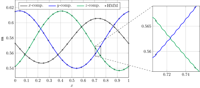
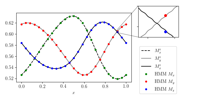
    The corresponding homogenized coefficient, which is not used in the HMM approach but as a reference solution, is 𝐀H=(∫011/a​(x)​𝑑x)βˆ’1β‰ˆ0.866superscript𝐀𝐻superscriptsuperscriptsubscript011π‘Žπ‘₯differential-dπ‘₯10.866\mathbf{A}^{H}=\left(\int_{0}^{1}1/a(x)dx\right)^{-1}\approx 0.866. In FigureΒ 1 the solution πŒΞ΅β€‹(x,T)superscriptπŒπœ€π‘₯𝑇\mathbf{M}^{\varepsilon}(x,T) at T=0.1𝑇0.1T=0.1 and the corresponding HMM approximation πŒβ€‹(x,T)𝐌π‘₯𝑇\mathbf{M}(x,T) computed on a grid with Δ​X=1/24Δ𝑋124\Delta X=1/24 are shown. Note that the HMM approximation agrees very well with 𝐌ΡsuperscriptπŒπœ€\mathbf{M}^{\varepsilon}.

    Refer to caption
    Figure 1: Solution 𝐦Ρsuperscriptπ¦πœ€\mathbf{m}^{\varepsilon} and corresponding HMM approximation to 1.1 with setup (EX1) at time T=0.1𝑇0.1T=0.1 when Ξ΅=1/200πœ€1200\varepsilon=1/200.
  • (EX2)

    For the first 2D example the initial data is

    𝐦init​(x)subscript𝐦initπ‘₯\displaystyle\mathbf{m}_{\mathrm{init}}(x) =~​𝐦​(x)/|~​𝐦​(x)|,absent~absent𝐦π‘₯~absent𝐦π‘₯\displaystyle=\tilde{}\mathbf{m}(x)/|\tilde{}\mathbf{m}(x)|,
    ~​𝐦​(x)~absent𝐦π‘₯\displaystyle\tilde{}\mathbf{m}(x) =[0.6+exp⁑(βˆ’0.3​(cos⁑(2​π​(x1βˆ’0.25))+cos⁑(2​π​(x2βˆ’0.12))))0.5+exp⁑(βˆ’0.4​(cos⁑(2​π​x1)+cos⁑(2​π​(x2βˆ’0.4))))0.4+exp⁑(βˆ’0.2​(cos⁑(2​π​(x1βˆ’0.81))+cos⁑(2​π​(x2βˆ’0.73))))],absentmatrix0.60.32πœ‹subscriptπ‘₯10.252πœ‹subscriptπ‘₯20.120.50.42πœ‹subscriptπ‘₯12πœ‹subscriptπ‘₯20.40.40.22πœ‹subscriptπ‘₯10.812πœ‹subscriptπ‘₯20.73\displaystyle=\begin{bmatrix}0.6+\exp(-0.3(\cos(2\pi(x_{1}-0.25))+\cos(2\pi(x_{2}-0.12))))\\ 0.5+\exp(-0.4(\cos(2\pi x_{1})+\cos(2\pi(x_{2}-0.4))))\\ 0.4+\exp(-0.2(\cos(2\pi(x_{1}-0.81))+\cos(2\pi(x_{2}-0.73))))\end{bmatrix},

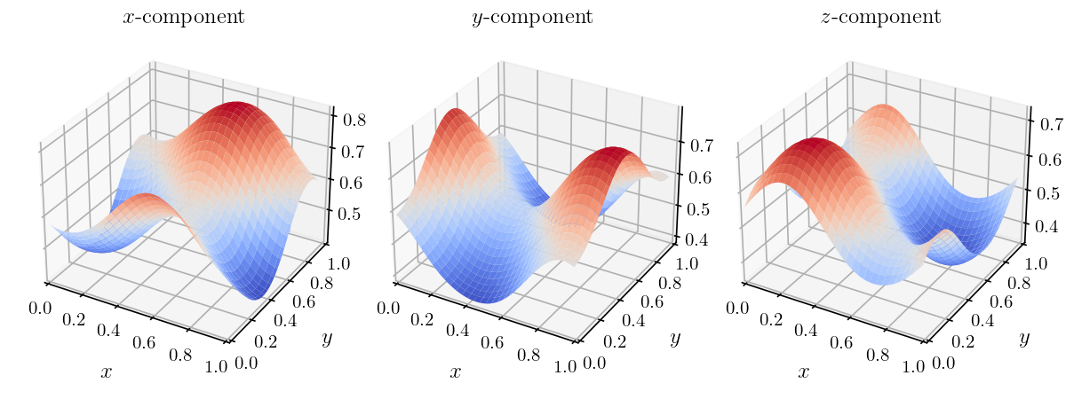
    which is shown in fig.Β 2. The material coefficient is given by

    a​(x)π‘Žπ‘₯\displaystyle a(x) =0.5+(0.5+0.25​sin⁑(2​π​x1))​(0.5+0.25​sin⁑(2​π​x2))absent0.50.50.252πœ‹subscriptπ‘₯10.50.252πœ‹subscriptπ‘₯2\displaystyle=0.5+(0.5+0.25\sin(2\pi x_{1}))(0.5+0.25\sin(2\pi x_{2}))
    +0.25​(cos⁑(2​π​(x1βˆ’x2))+sin⁑(2​π​x1)),0.252πœ‹subscriptπ‘₯1subscriptπ‘₯22πœ‹subscriptπ‘₯1\displaystyle\qquad+0.25(\cos(2\pi(x_{1}-x_{2}))+\sin(2\pi x_{1})),

    which corresponds to a homogenized coefficient with non-zero off-diagonal elements,

    𝐀Hβ‰ˆ[0.6170.0260.0260.715].superscript𝐀𝐻matrix0.6170.0260.0260.715\mathbf{A}^{H}\approx\begin{bmatrix}0.617&0.026\\ 0.026&0.715\end{bmatrix}.

    For this example, 𝐀Hsuperscript𝐀𝐻\mathbf{A}^{H} has to be computed numerically (with high precision).
    Refer to caption
    Figure 2: Initial data 𝐌initsubscript𝐌init\mathbf{M}_{\mathrm{init}} for the 2D problems
  • (EX3)

    The second 2D example has the same initial data as (EX2) but a different material coefficient,

    a​(x)=(1.1+0.5​sin⁑(2​π​x1))​(1.1+0.5​sin⁑(2​π​x2)).π‘Žπ‘₯1.10.52πœ‹subscriptπ‘₯11.10.52πœ‹subscriptπ‘₯2a(x)=(1.1+0.5\sin(2\pi x_{1}))(1.1+0.5\sin(2\pi x_{2})).

    The corresponding homogenized matrix can be computed analytically [6] and takes the value

    𝐀H=1.1​1.12βˆ’0.25β€‹πˆ.superscript𝐀𝐻1.1superscript1.120.25𝐈\mathbf{A}^{H}=1.1\sqrt{1.1^{2}-0.25}\mathbf{I}.

In all three cases, it holds that aΡ​(x)=a​(x/Ξ΅)superscriptπ‘Žπœ€π‘₯π‘Žπ‘₯πœ€a^{\varepsilon}(x)=a(x/\varepsilon).

3 Time stepping for Landau-Lifshitz problems

A variety of different methods for time integration of the Landau-Lifshitz equation in a finite difference setting are available, as for example discussed in the review articles [16, 9, 7]. Most of these methods can be characterized as either projection methods or geometric integrators, typically based on the implicit midpoint method. In a projection method, the basic update procedure does not preserve the length of the magnetization vector moments which makes it necessary to project the intermediate result back to the unit sphere at the end of each time step. Commonly used examples for this kind of methods are projection versions of Runge-Kutta methods as well as the Gauss-Sequel projection method [30, 24]. Furthermore, an implicit projection method based on a linear update formula is proposed in [14].

The most common geometric integrator is the implicit midpoint method, which is both norm preserving and in case of no damping, Ξ±=0𝛼0\alpha=0, also energy conserving [10, 11]. However, since it is computationally rather expensive, several semi-implicit variations have been proposed, in particular SIA and SIB introduced in [26] as well as the midpoint extrapolation method, MPE, [29]. Further geometric integrators are the Cayley transform based approaches discussed in [23, 19].

While there are many methods available for time integration of the Landau-Lifshitz equation, which have advantages in different scenarios, we here have a strong focus on computational cost, especially when considering the micro problem, where the subsequent averaging process reduces the importance of conservation of physical properties. For the HMM macro model, the form of the problem, 2.8, prevents the rewriting of the equation as would be necessary for some integrators, for example the method in [14]. In general, the dependence of 𝐇avgsubscript𝐇avg\mathbf{H}_{\mathrm{avg}} in 2.8 on the micro solution makes the use of implicit methods problematic, as is further discussed in SectionΒ 3.3.

In the following, we focus on several time integration methods that might be suitable for the given setup and then motivate our choice for the macro and micro problem, respectively.

3.1 Description of selected methods

The methods we focus on are two projection methods, HeunP and RK4P, as well as the semi-implicit midpoint extrapolation method, MPE, introduced in [29] and MPEA, an adaption of the latter method. We furthermore include the implicit midpoint method in the considerations since it can be seen as a reference method for time integration of the Landau-Lifshitz equation.

In this section, we suppose that we work with a discrete grid in space with locations xi=x0+i​Δ​xsubscriptπ‘₯𝑖subscriptπ‘₯0𝑖Δπ‘₯x_{i}=x_{0}+i\Delta x, where i∈{0,…,N}d𝑖superscript0…𝑁𝑑i\in\{0,...,N\}^{d}, and consider time points tj=t0+j​Δ​tsubscript𝑑𝑗subscript𝑑0𝑗Δ𝑑t_{j}=t_{0}+j\Delta t, j=0,…,M𝑗0…𝑀j=0,...,M. We denote by 𝐦ijβˆˆβ„3superscriptsubscript𝐦𝑖𝑗superscriptℝ3\mathbf{m}_{i}^{j}\in\mathbb{R}^{3} an approximation to the magnetization at location xisubscriptπ‘₯𝑖x_{i} and time tjsubscript𝑑𝑗t_{j}, 𝐦ijβ‰ˆπ¦β€‹(xi,tj)superscriptsubscript𝐦𝑖𝑗𝐦subscriptπ‘₯𝑖subscript𝑑𝑗\mathbf{m}_{i}^{j}\approx\mathbf{m}(x_{i},t_{j}). When writing 𝐦jsuperscript𝐦𝑗\mathbf{m}^{j} we refer to a vector in ℝ3​Ndsuperscriptℝ3superscript𝑁𝑑\mathbb{R}^{3N^{d}} that contains all 𝐦ijsuperscriptsubscript𝐦𝑖𝑗\mathbf{m}_{i}^{j}. In the main part of this section, we do not distinguish between macro and micro problem but focus on the general behavior of the time stepping methods. Thus, 𝐦𝐦\mathbf{m} can denote both a micro or macro solution.

We furthermore use the notation 𝐟i​(𝐦j)subscriptπŸπ‘–superscript𝐦𝑗\mathbf{f}_{i}(\mathbf{m}^{j}) to denote the value of a function 𝐟𝐟\mathbf{f} at location xisubscriptπ‘₯𝑖x_{i} which might depend on the values of 𝐦jsuperscript𝐦𝑗\mathbf{m}^{j} at several space locations. In particular, we write 𝐇i​(𝐦j)subscript𝐇𝑖superscript𝐦𝑗\mathbf{H}_{i}(\mathbf{m}^{j}) to denote a discrete approximation to the effective field at xisubscriptπ‘₯𝑖x_{i}. On the macro scale, it thus holds that 𝐇i​(𝐦j)β‰ˆπ‡avg​(xi,tj;Β―β€‹πŒ)subscript𝐇𝑖superscript𝐦𝑗subscript𝐇avgsubscriptπ‘₯𝑖subscript𝑑𝑗¯absent𝐌\mathbf{H}_{i}(\mathbf{m}^{j})\approx\mathbf{H}_{\mathrm{avg}}(x_{i},t_{j};\bar{}\mathbf{M}) or, when considering the corresponding homogenized problem in case of a periodic material coefficient,

𝐇i​(𝐦j)β‰ˆβˆ‡β‹…(βˆ‡π¦β€‹(xi,tj)​𝐀H).subscript𝐇𝑖superscript𝐦𝑗⋅bold-βˆ‡bold-βˆ‡π¦subscriptπ‘₯𝑖subscript𝑑𝑗superscript𝐀𝐻\mathbf{H}_{i}(\mathbf{m}^{j})\approx\boldsymbol{\nabla}\cdot(\boldsymbol{\nabla}\mathbf{m}(x_{i},t_{j})\mathbf{A}^{H}).

For the micro problem, we have

𝐇i​(𝐦j)β‰ˆβˆ‡β‹…(a​(xi/Ξ΅)β€‹βˆ‡π¦Ξ΅β€‹(xi,tj)).subscript𝐇𝑖superscript𝐦𝑗⋅bold-βˆ‡π‘Žsubscriptπ‘₯π‘–πœ€bold-βˆ‡superscriptπ¦πœ€subscriptπ‘₯𝑖subscript𝑑𝑗\mathbf{H}_{i}(\mathbf{m}^{j})\approx\boldsymbol{\nabla}\cdot(a(x_{i}/\varepsilon)\boldsymbol{\nabla}\mathbf{m}^{\varepsilon}(x_{i},t_{j})).

The particular form of 𝐇i​(𝐦j)subscript𝐇𝑖superscript𝐦𝑗\mathbf{H}_{i}(\mathbf{m}^{j}) does not have a major influence on the following discussions if not explicitly stated otherwise.

HeunP and RK4P

HeunP and RK4P are the standard Runge Kutta 2 and Runge Kutta 4 methods with an additional projection back to the unit sphere at the end of every time step. Let πŸβ€‹(𝐦j)𝐟superscript𝐦𝑗\mathbf{f}(\mathbf{m}^{j}) be the 3​Nd3superscript𝑁𝑑{3N^{d}}-vector such that

𝐟i​(𝐦j):=βˆ’π¦ij×𝐇i​(𝐦j)βˆ’Ξ±β€‹π¦ij×𝐦ij×𝐇i​(𝐦j),i∈{0,…,N}d.formulae-sequenceassignsubscriptπŸπ‘–superscript𝐦𝑗superscriptsubscript𝐦𝑖𝑗subscript𝐇𝑖superscript𝐦𝑗𝛼superscriptsubscript𝐦𝑖𝑗superscriptsubscript𝐦𝑖𝑗subscript𝐇𝑖superscript𝐦𝑗𝑖superscript0…𝑁𝑑\mathbf{f}_{i}(\mathbf{m}^{j}):=-\mathbf{m}_{i}^{j}\times\mathbf{H}_{i}(\mathbf{m}^{j})-\alpha\mathbf{m}_{i}^{j}\times\mathbf{m}_{i}^{j}\times\mathbf{H}_{i}(\mathbf{m}^{j}),\qquad i\in\{0,...,N\}^{d}.

Then in the Runge-Kutta methods, one computes stage values

𝐀1=πŸβ€‹(𝐦j),𝐀2=πŸβ€‹(𝐦j+Δ​t2​𝐀1),𝐀2=πŸβ€‹(𝐦j+Δ​t2​𝐀2),𝐀4=πŸβ€‹(𝐦j+Δ​t​𝐀3).formulae-sequencesubscript𝐀1𝐟superscript𝐦𝑗formulae-sequencesubscript𝐀2𝐟superscript𝐦𝑗Δ𝑑2subscript𝐀1formulae-sequencesubscript𝐀2𝐟superscript𝐦𝑗Δ𝑑2subscript𝐀2subscript𝐀4𝐟superscript𝐦𝑗Δ𝑑subscript𝐀3\displaystyle\mathbf{k}_{1}=\mathbf{f}(\mathbf{m}^{j}),\quad\mathbf{k}_{2}=\mathbf{f}(\mathbf{m}^{j}+\tfrac{\Delta t}{2}\mathbf{k}_{1}),\quad\mathbf{k}_{2}=\mathbf{f}(\mathbf{m}^{j}+\tfrac{\Delta t}{2}\mathbf{k}_{2}),\quad\mathbf{k}_{4}=\mathbf{f}(\mathbf{m}^{j}+\Delta t\mathbf{k}_{3}).

In HeunP (RK2P), the time step update then is given by

𝐦ij+1=~​𝐦i/|~​𝐦i|,where~​𝐦=𝐦j+Δ​t2​(𝐀1+𝐀2),formulae-sequencesubscriptsuperscript𝐦𝑗1𝑖~absentsubscript𝐦𝑖~absentsubscript𝐦𝑖where~absent𝐦superscript𝐦𝑗Δ𝑑2subscript𝐀1subscript𝐀2\displaystyle\mathbf{m}^{j+1}_{i}=\tilde{}\mathbf{m}_{i}/|\tilde{}\mathbf{m}_{i}|,\qquad\text{where}\qquad\tilde{}\mathbf{m}=\mathbf{m}^{j}+\tfrac{\Delta t}{2}(\mathbf{k}_{1}+\mathbf{k}_{2}), (3.15)

and for RK4P,

𝐦ij+1=~​𝐦i/|~​𝐦i|,where~​𝐦=𝐦j+Δ​t6​(𝐀1+2​𝐀2+2​𝐀3+𝐀4).formulae-sequencesubscriptsuperscript𝐦𝑗1𝑖~absentsubscript𝐦𝑖~absentsubscript𝐦𝑖where~absent𝐦superscript𝐦𝑗Δ𝑑6subscript𝐀12subscript𝐀22subscript𝐀3subscript𝐀4\displaystyle\mathbf{m}^{j+1}_{i}=\tilde{}\mathbf{m}_{i}/|\tilde{}\mathbf{m}_{i}|,\qquad\text{where}\qquad\tilde{}\mathbf{m}=\mathbf{m}^{j}+\tfrac{\Delta t}{6}(\mathbf{k}_{1}+2\mathbf{k}_{2}+2\mathbf{k}_{3}+\mathbf{k}_{4}). (3.16)

HeunP is a second order method and RK4P is fourth order accurate.

Implicit midpoint

Using the implicit midpoint method, the Landau-Lifshitz equation is discretized as

𝐦ij+1βˆ’π¦ijΔ​t=βˆ’π¦ij+𝐦ij+12×𝐑i​(𝐦j+𝐦j+12),superscriptsubscript𝐦𝑖𝑗1superscriptsubscript𝐦𝑖𝑗Δ𝑑superscriptsubscript𝐦𝑖𝑗superscriptsubscript𝐦𝑖𝑗12subscript𝐑𝑖superscript𝐦𝑗superscript𝐦𝑗12\frac{\mathbf{m}_{i}^{j+1}-\mathbf{m}_{i}^{j}}{\Delta t}=-\frac{\mathbf{m}_{i}^{j}+\mathbf{m}_{i}^{j+1}}{2}\times\mathbf{h}_{i}\left(\frac{\mathbf{m}^{j}+\mathbf{m}^{j+1}}{2}\right), (3.17)

where

𝐑i​(𝐦):=𝐇i​(𝐦)+α​𝐦i×𝐇i​(𝐦).assignsubscript𝐑𝑖𝐦subscript𝐇𝑖𝐦𝛼subscript𝐦𝑖subscript𝐇𝑖𝐦\mathbf{h}_{i}(\mathbf{m}):=\mathbf{H}_{i}(\mathbf{m})+\alpha\mathbf{m}_{i}\times\mathbf{H}_{i}(\mathbf{m}). (3.18)

Hence, the values for 𝐦ij+1superscriptsubscript𝐦𝑖𝑗1\mathbf{m}_{i}^{j+1} are obtained by solving the nonlinear system

𝐦j+1=(𝐈+Δ​t2​[𝐑​(𝐦j+𝐦j+12)]Γ—)βˆ’1​(πˆβˆ’Ξ”β€‹t2​[𝐑​(𝐦j+𝐦j+12)]Γ—)​𝐦j,superscript𝐦𝑗1superscriptπˆΞ”π‘‘2subscriptdelimited-[]𝐑superscript𝐦𝑗superscript𝐦𝑗121πˆΞ”π‘‘2subscriptdelimited-[]𝐑superscript𝐦𝑗superscript𝐦𝑗12superscript𝐦𝑗\mathbf{m}^{j+1}=\left(\mathbf{I}+\frac{\Delta t}{2}\left[\mathbf{h}\left(\frac{\mathbf{m}^{j}+\mathbf{m}^{j+1}}{2}\right)\right]_{\times}\right)^{-1}\left(\mathbf{I}-\frac{\Delta t}{2}\left[\mathbf{h}\left(\frac{\mathbf{m}^{j}+\mathbf{m}^{j+1}}{2}\right)\right]_{\times}\right)\mathbf{m}^{j}, (3.19)

where [𝐑]Γ—subscriptdelimited-[]𝐑\left[\mathbf{h}\right]_{\times} is the matrix such that the matrix-vector product [𝐑]×​𝐦jsubscriptdelimited-[]𝐑superscript𝐦𝑗\left[\mathbf{h}\right]_{\times}\mathbf{m}^{j} corresponds to taking the cross products 𝐑i×𝐦ijsubscript𝐑𝑖superscriptsubscript𝐦𝑖𝑗\mathbf{h}_{i}\times\mathbf{m}_{i}^{j} for all i∈{0,…,N}d𝑖superscript0…𝑁𝑑i\in\{0,...,N\}^{d}. The implicit midpoint method is norm-conserving and results in a second order accurate approximation.

However, when using Newton’s method to solve the non-linear system 3.19, one has to compute the Jacobian of the right-hand side with respect to 𝐦j+1superscript𝐦𝑗1\mathbf{m}^{j+1}, a sparse, but not (block)-diagonal, 3​NdΓ—3​Nd3superscript𝑁𝑑3superscript𝑁𝑑{3N^{d}\times 3N^{d}} matrix and then solve the corresponding linear system in each iteration, which has a rather high computational cost. In case of the HMM macro model, the Jacobian cannot be computed analytically since then 𝐇isubscript𝐇𝑖\mathbf{H}_{i} in 3.18 is replaced by the averaged quantity 𝐇avg​(xi,tj;𝐦)subscript𝐇avgsubscriptπ‘₯𝑖subscript𝑑𝑗𝐦\mathbf{H}_{\mathrm{avg}}(x_{i},t_{j};\mathbf{m}), with a dependence on 𝐦𝐦\mathbf{m} that is very complicated. A numerical approximation is highly expensive since it means solving C​N2​d𝐢superscript𝑁2𝑑CN^{2d} additional micro problems per time step.

MPE and MPEA

As described in [29], the idea behind the midpoint extrapolation method is to approximate 𝐑​(𝐦j+𝐦j+12)𝐑superscript𝐦𝑗superscript𝐦𝑗12\mathbf{h}(\frac{\mathbf{m}^{j}+\mathbf{m}^{j+1}}{2}) in 3.17 using the explicit extrapolation formula

𝐑​(𝐦j+𝐦j+12)β‰ˆπ‘j+1/2:=32​𝐑​(𝐦j)βˆ’12​𝐑​(𝐦jβˆ’1).𝐑superscript𝐦𝑗superscript𝐦𝑗12superscript𝐑𝑗12assign32𝐑superscript𝐦𝑗12𝐑superscript𝐦𝑗1\mathbf{h}\left(\frac{\mathbf{m}^{j}+\mathbf{m}^{j+1}}{2}\right)\approx\mathbf{h}^{j+1/2}:=\tfrac{3}{2}\mathbf{h}(\mathbf{m}^{j})-\tfrac{1}{2}\mathbf{h}(\mathbf{m}^{j-1}). (3.20)

The update for 𝐦isubscript𝐦𝑖\mathbf{m}_{i} then becomes

𝐦ij+1βˆ’π¦ijΔ​t=βˆ’π¦ij+𝐦ij+12×𝐑ij+1/2.superscriptsubscript𝐦𝑖𝑗1superscriptsubscript𝐦𝑖𝑗Δ𝑑superscriptsubscript𝐦𝑖𝑗superscriptsubscript𝐦𝑖𝑗12superscriptsubscript𝐑𝑖𝑗12\frac{\mathbf{m}_{i}^{j+1}-\mathbf{m}_{i}^{j}}{\Delta t}=-\frac{\mathbf{m}_{i}^{j}+\mathbf{m}_{i}^{j+1}}{2}\times\mathbf{h}_{i}^{j+1/2}. (3.21)

The quantity 𝐑ij+1/2superscriptsubscript𝐑𝑖𝑗12\mathbf{h}_{i}^{j+1/2} here is independent of 𝐦j+1superscript𝐦𝑗1\mathbf{m}^{j+1}, which means that the problem decouples into Ndsuperscript𝑁𝑑N^{d} small 3Γ—3333\times 3 systems. Since the first term on the right-hand side still contains 𝐦ij+1superscriptsubscript𝐦𝑖𝑗1\mathbf{m}_{i}^{j+1}, this is considered a semi-implicit method. Just as the implicit midpoint method, MPE is second order accurate. We furthermore propose to use third-order accurate extrapolation,

𝐑j+1/2:=2312​𝐑​(𝐦j)βˆ’1612​𝐑​(𝐦jβˆ’1)+512​𝐑​(𝐦jβˆ’2),assignsuperscript𝐑𝑗122312𝐑superscript𝐦𝑗1612𝐑superscript𝐦𝑗1512𝐑superscript𝐦𝑗2\mathbf{h}^{j+1/2}:=\frac{23}{12}\mathbf{h}(\mathbf{m}^{j})-\frac{16}{12}\mathbf{h}(\mathbf{m}^{j-1})+\frac{5}{12}\mathbf{h}(\mathbf{m}^{j-2}), (3.22)

in 3.21, which gives MPEA, the adapted MPE method. As it is based on the implicit midpoint method, MPEA is second order accurate just like MPE, but has better stability properties for low damping, as shown in the next section.

As MPE and MPEA are multi-step methods, values for 𝐦1superscript𝐦1\mathbf{m}^{1} (and 𝐦2superscript𝐦2\mathbf{m}^{2}) are required for startup. These can be obtained using HeunP or RK4P, as suggested in [29].

Comparison of methods

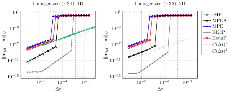
In Figure 3, the error with respect to a reference solution 𝐦refsubscript𝐦ref\mathbf{m}_{\mathrm{ref}} is shown for all the considered (semi-)explicit methods and two example problems, a 1D problem and a 2D problem. Both example problems are homogenized problems on a rather coarse spatial discretization grid such as we might have in the HMM macro problem. For the 1D problem, the implicit midpoint method is also included for reference.
Refer to caption
Figure 3: Comparison of L2superscript𝐿2L^{2}-error in different time stepping methods when varying the time step size Δ​tΔ𝑑\Delta t given a fixed spatial discretization with Δ​x=1/50Ξ”π‘₯150\Delta x=1/50 and damping parameter Ξ±=0.01𝛼0.01\alpha=0.01. The dotted vertical line corresponds to Δ​t=(Δ​x)2Δ𝑑superscriptΞ”π‘₯2\Delta t=(\Delta x)^{2} in each case.

For small time step sizes, one can observe the expected convergence rates for HeunP, RK4P and MPE. For MPEA, we observe third order convergence in the 1D problem, while in the 2D case, we have second order convergence for small Δ​tΔ𝑑\Delta t. Overall, MPEA results in lower errors compared to HeunP, MPE and the implicit midpoint method. RK4P is most accurate.

3.2 Stability of the time stepping methods

It is well known that in explicit time stepping methods for the Landau-Lifshitz equation, the choice of time step size Δ​tΔ𝑑\Delta t given Δ​xΞ”π‘₯\Delta x in space is severely constrained by numerical stability, see for example [30, 7]. Note that due to the norm preservation property of the considered methods, the solutions cannot grow arbitrarily as unstable solutions typically do in other applications. However, when taking too large time steps, explicit time integration will typically result in solutions that oscillate rapidly and do not represent the intended solution in any way. Following standard practice in the field, we refer to this behavior as instability in this section. This stability limit is seen clearly for all methods expect IMP in FigureΒ 3.

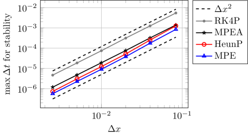
In numerical experiments, we observe that in order to obtain stable solutions, the time step size Δ​tΔ𝑑\Delta t has to be chosen proportional to Δ​x2Ξ”superscriptπ‘₯2\Delta x^{2} for all of the considered methods, both explicit and semi-explicit. This is exemplified in FigureΒ 4 for (EX1) with Ξ±=0.01𝛼0.01\alpha=0.01.

Refer to caption
Figure 4: Empirically found maximum value of Δ​tΔ𝑑\Delta t that still results in a stable solution for varying values of Δ​xΞ”π‘₯\Delta x in (EX1), homogenized, with Ξ±=0.01𝛼0.01\alpha=0.01.

To get a better understanding of stability, consider a semi-discrete form of the Landau-Lifshitz equation in one dimension with a constant material coefficient, equal to one. This can be written as

βˆ‚t𝐦=πŸΞ±β€‹(𝐦),πŸΞ±β€‹(𝐦)=βˆ’π¦Γ—Dβ€‹π¦βˆ’Ξ±β€‹π¦Γ—π¦Γ—D​𝐦=βˆ’B​(𝐦)​D​𝐦,formulae-sequencesubscript𝑑𝐦subscriptπŸπ›Όπ¦subscriptπŸπ›Όπ¦π¦π·π¦π›Όπ¦π¦π·π¦π΅π¦π·π¦\partial_{t}\mathbf{m}=\mathbf{f}_{\alpha}(\mathbf{m}),\qquad\mathbf{f}_{\alpha}(\mathbf{m})=-\mathbf{m}\times{D}\mathbf{m}-\alpha\mathbf{m}\times\mathbf{m}\times{D}\mathbf{m}=-B(\mathbf{m})D\mathbf{m}, (3.23)

where π¦βˆˆβ„3​N𝐦superscriptℝ3𝑁\mathbf{m}\in\mathbb{R}^{3N} contains the vectors {𝐦i}subscript𝐦𝑖\{\mathbf{m}_{i}\}, D𝐷D is the discrete Laplacian and B​(𝐦)𝐡𝐦B(\mathbf{m}) is a block diagonal skew-symmetric matrix with eigenvalues {0,+iβˆ’Ξ±,βˆ’iβˆ’Ξ±}0𝑖𝛼𝑖𝛼\{0,\ +i-\alpha,\ -i-\alpha\} that comes from the cross products. If {𝐦i}subscript𝐦𝑖\{\mathbf{m}_{i}\} samples a smooth function, the Jacobian of πŸΞ±β€‹(𝐦)subscriptπŸπ›Όπ¦\mathbf{f}_{\alpha}(\mathbf{m}) can be approximated as

βˆ‡π¦πŸΞ±β€‹(𝐦)=βˆ’βˆ‡π¦B​(𝐦)​Dβ€‹π¦β‰ˆβˆ’B​(𝐦)​D.subscriptβˆ‡π¦subscriptπŸπ›Όπ¦subscriptβˆ‡π¦π΅π¦π·π¦π΅π¦π·\nabla_{\mathbf{m}}\mathbf{f}_{\alpha}(\mathbf{m})=-\nabla_{\mathbf{m}}B(\mathbf{m})D\mathbf{m}\approx-B(\mathbf{m})D.

Still assuming smoothness, one can subsequently deduce [20] that the eigenvalues of the Jacobian are approximately given as the eigenvalues Ο‰πœ”\omega of βˆ’D𝐷-D multiplied by the eigenvalues of B​(𝐦)𝐡𝐦B(\mathbf{m}), namely

Ξ»+β‰ˆ(iβˆ’Ξ±)​ω,Ξ»βˆ’β‰ˆ(βˆ’iβˆ’Ξ±)​ω,Ξ»0β‰ˆ0.formulae-sequencesubscriptπœ†π‘–π›Όπœ”formulae-sequencesubscriptπœ†π‘–π›Όπœ”subscriptπœ†00\lambda_{+}\approx(i-\alpha)\omega,\qquad\lambda_{-}\approx(-i-\alpha)\omega,\qquad\lambda_{0}\approx 0.

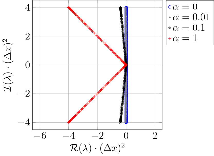
The eigenvalues of βˆ’D𝐷-D, the negative discrete Laplacian, are real, positive and bounded by O​(Δ​xβˆ’2)𝑂Δsuperscriptπ‘₯2O(\Delta x^{-2}). Consequently, the eigenvalues of the Jacobian βˆ‡π¦πŸΞ±β€‹(𝐦)subscriptβˆ‡π¦subscriptπŸπ›Όπ¦\nabla_{\mathbf{m}}\mathbf{f}_{\alpha}(\mathbf{m}) will lie along the lines s​(Β±iβˆ’Ξ±)𝑠plus-or-minus𝑖𝛼s(\pm i-\alpha) for real s∈[0,O(Ξ”xβˆ’2)s\in[0,O(\Delta x^{-2})] in the complex plane. This is illustrated in FigureΒ 5(a) where we have plotted the eigenvalues of βˆ‡π¦πŸΞ±β€‹(𝐦)subscriptβˆ‡π¦subscriptπŸπ›Όπ¦\nabla_{\mathbf{m}}\mathbf{f}_{\alpha}(\mathbf{m}), scaled by Δ​x2Ξ”superscriptπ‘₯2\Delta x^{2}, for several values of α𝛼\alpha. One can observe that given Ξ±=0𝛼0\alpha=0, the eigenvalues are purely imaginary. As α𝛼\alpha increases, the real parts of the eigenvalues decrease correspondingly.

For the Landau-Lifshitz equation 2.2 with a material coefficient as well as the homogenized equation 2.3, the eigenvalues of the corresponding Jacobians get a different scaling based on the material coefficient but their general behavior is not affected. We hence conjecture that it is necessary that

Δ​t(Δ​x)2≀Cstab,Ξ±,Δ𝑑superscriptΞ”π‘₯2subscript𝐢stab𝛼\displaystyle\frac{\Delta t}{(\Delta x)^{2}}\leq C_{\mathrm{stab},\alpha}, (3.24)

where Cstab,Ξ±subscript𝐢stab𝛼C_{\mathrm{stab},\alpha} is a constant depending on the chosen integrator, the damping parameter α𝛼\alpha and the material coefficient. Based on several numerical examples, we observe for the latter dependence that

Cstab,α≲Cα​{(maxy∈Y⁑|a​(y)|)βˆ’1,original problem,(maxi,j⁑|Ai​jH|)βˆ’1,homogenized problem,less-than-or-similar-tosubscript𝐢stab𝛼subscript𝐢𝛼casessuperscriptsubscriptπ‘¦π‘Œπ‘Žπ‘¦1original problemsuperscriptsubscript𝑖𝑗subscriptsuperscript𝐴𝐻𝑖𝑗1homogenized problemC_{\mathrm{stab},\alpha}\lesssim C_{\mathrm{\alpha}}\begin{cases}(\max_{y\in Y}|a(y)|)^{-1},&\text{original problem},\\ (\max_{i,j}|A^{H}_{ij}|)^{-1},&\text{homogenized problem},\end{cases}

where CΞ±subscript𝐢𝛼C_{\mathrm{\alpha}} denotes further dependence on α𝛼\alpha and the integrator.

Stability regions of related methods

In order to better understand the stability behavior of the considered time integrators, it is beneficial to study the stability regions of some well-known, related methods. For HeunP and RK4P, we regard the corresponding integrators without projection. We observe a very similar stability behavior when using Heun and RK4 to solve the problems considered in FiguresΒ 3 andΒ 4.

To get some intuition about MPE(A), we start by considering the problem

βˆ‚t𝐦=βˆ’π§Γ—π‡β€‹(𝐦)βˆ’Ξ±β€‹π§Γ—π¦Γ—π‡β€‹(𝐦)=βˆ’π§Γ—π‘β€‹(𝐦),subscript𝑑𝐦𝐧𝐇𝐦𝛼𝐧𝐦𝐇𝐦𝐧𝐑𝐦\displaystyle\partial_{t}\mathbf{m}=-\mathbf{n}\times\mathbf{H}(\mathbf{m})-\alpha\mathbf{n}\times\mathbf{m}\times\mathbf{H}(\mathbf{m})=-\mathbf{n}\times\mathbf{h}(\mathbf{m}), (3.25)

where 𝐧𝐧\mathbf{n} is a given vector function, constant in time, with |𝐧|=1𝐧1|\mathbf{n}|=1. This corresponds to replacing the first 𝐦𝐦\mathbf{m} in each term on the right-hand side in 2.2 by a constant approximation. For this problem, time stepping according to the MPE update 3.21 results in

𝐦ij+1βˆ’π¦ijΔ​t=βˆ’π§i×𝐑ij+1/2=βˆ’32​(𝐧i×𝐑i​(𝐦j))+12​(𝐧i×𝐑i​(𝐦jβˆ’1)).superscriptsubscript𝐦𝑖𝑗1superscriptsubscript𝐦𝑖𝑗Δ𝑑subscript𝐧𝑖superscriptsubscript𝐑𝑖𝑗1232subscript𝐧𝑖subscript𝐑𝑖superscript𝐦𝑗12subscript𝐧𝑖subscript𝐑𝑖superscript𝐦𝑗1\frac{\mathbf{m}_{i}^{j+1}-\mathbf{m}_{i}^{j}}{\Delta t}=-\mathbf{n}_{i}\times\mathbf{h}_{i}^{j+1/2}=-\frac{3}{2}\left(\mathbf{n}_{i}\times\mathbf{h}_{i}(\mathbf{m}^{j})\right)+\frac{1}{2}\left(\mathbf{n}_{i}\times\mathbf{h}_{i}(\mathbf{m}^{j-1})\right). (3.26)

This is the same update scheme as one gets when applying the Adams-Bashforth 2 (AB2) method to 3.25. In the same way, MPEA and AB3 are connected. Furthermore, note that the term that was replaced by 𝐧𝐧\mathbf{n} in 2.2 to obtain 3.25 is the one that is treated implicitly in the semi-implicit methods MPE(A). We hence expect that studying the stability of AB2(3) can give an indication of what to expect for MPE(A). This is backed up by the fact that the stability properties observed for MPE(A) in Figures 3 and 4 are closely matched when using AB2(3) to solve the respective problems.

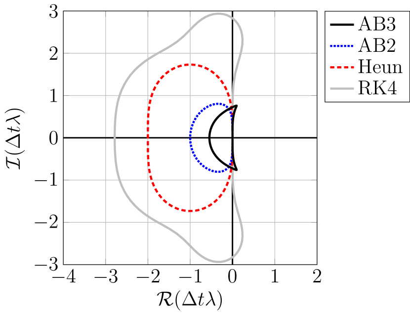
When comparing the stability regions of RK4, Heun, AB2 and AB3 as shown in FigureΒ 5(b), one clearly sees that the Runge-Kutta methods have larger stability regions than the multi-step methods. RK4’s stability region is largest and contains part of the imaginary axis, while the one for Heun is only close to the imaginary axis in a shorter interval.
Refer to caption
(a) Eigenvalues of the Jacobian βˆ‡πŸΞ±β€‹(𝐦)βˆ‡subscriptπŸπ›Όπ¦\nabla\mathbf{f}_{\alpha}(\mathbf{m}) for several values of α𝛼\alpha
Refer to caption
(b) Stability regions of RK2 (Heun), RK4 as well as AB2 and AB3.
Figure 5: Eigenvalues of Jacobian βˆ‡πŸΞ±β€‹(𝐦)βˆ‡subscriptπŸπ›Όπ¦\nabla\mathbf{f}_{\alpha}(\mathbf{m}) and stability regions of methods related to the considered time integrators.

AB2 and AB3 have stability regions with a similar extent in the imaginary direction, but while AB3’s contains part of the imaginary axis, AB2’s does not. On the other hand, the stability region of AB2 is wider in the real direction.

Consider now again the example problems shown in FigureΒ 3 where Ξ±=0.01𝛼0.01\alpha=0.01, which implies that the eigenvalues of the corresponding Jacobian are rather close to the imaginary axis. Based on FigureΒ 5(b) we therefore expect the methods with related stability areas which include parts of the imaginary axis, RK4P and MPEA, to require fewer time steps than HeunP and MPE. This matches with the observed stability behavior in FigureΒ 3.

Influence of α𝛼\alpha

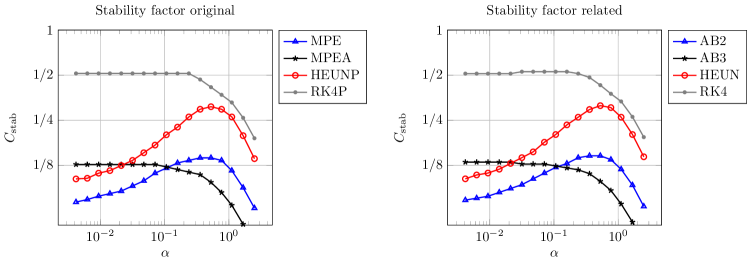
To further investigate the influence of α𝛼\alpha on Cstab,Ξ±subscript𝐢stab𝛼C_{\mathrm{stab,\alpha}}, this factor is shown in FigureΒ 6 for varying α𝛼\alpha, both for the considered methods HeunP, RK4P, MPE and MPEA and the discussed related methods, Heun, RK4, AB2 and AB3. The behavior of Cstab,Ξ±subscript𝐢stab𝛼C_{\mathrm{stab,\alpha}} is almost the same for the actual and the related methods.

As expected, we observe that Cstab,Ξ±subscript𝐢stab𝛼C_{\mathrm{stab,\alpha}} for low α𝛼\alpha-values is constant for MPEA and RK4P, with related stability regions that include the imaginary axis, while for HeunP and MPE, lower α𝛼\alpha results in lower Cstab,Ξ±subscript𝐢stab𝛼C_{\mathrm{stab,\alpha}}. When increasing α𝛼\alpha, the eigenvalues of βˆ‡m𝐟αsubscriptbold-βˆ‡π‘šsubscriptπŸπ›Ό\boldsymbol{\nabla}_{m}\mathbf{f}_{\alpha} as defined in 3.23 get larger real parts and the stability regions’ extent in the real direction becomes more important. For RK4P and MPEA, this means that for α≳0.2greater-than-or-equivalent-to𝛼0.2\alpha\gtrsim 0.2, Cstab,Ξ±subscript𝐢stab𝛼C_{\mathrm{stab,\alpha}} decreases as α𝛼\alpha increases. For HeunP and MPE, the highest Cstab,Ξ±subscript𝐢stab𝛼C_{\mathrm{stab,\alpha}} is obtained around Ξ±=0.5𝛼0.5\alpha=0.5. For higher α𝛼\alpha, the required Cstab,Ξ±subscript𝐢stab𝛼C_{\mathrm{stab,\alpha}} decreases as α𝛼\alpha increases. Overall, MPEA requires the lowest Cstab,Ξ±subscript𝐢stab𝛼C_{\mathrm{stab},\alpha} for high α𝛼\alpha, which agrees with the fact that the related stability region is shortest in the real direction. The highest Cstab,Ξ±subscript𝐢stab𝛼C_{\mathrm{stab},\alpha} is still the one for RK4P, in accordance with the stability region considerations.
Refer to caption
Figure 6: Dependence of Cstab,Ξ±subscript𝐢stab𝛼C_{\mathrm{stab},\alpha} on α𝛼\alpha, for actual and related time integrators. Based on the homogenized solution to (EX2).

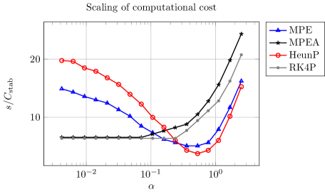
However, HeunP is a two-stage method and each RK4P step consists of four stages, while MPE and MPEA are multi-step methods that only require computation of one new stage per time step. In general, each step of HeunP/RK4P thus has roughly two/four times the computational cost as a MPE(A) step. To take this into account, we compare the total number of computations for each method by considering the factor s/Cstab,α𝑠subscript𝐢stab𝛼s/C_{\mathrm{stab},\alpha}, where s𝑠s denotes the number of stages in the method. This is shown in FigureΒ 7.

Refer to caption
Figure 7: Left: Dependence of Cstab,Ξ±subscript𝐢stab𝛼C_{\mathrm{stab},\alpha} on α𝛼\alpha, based on the homogenized solution to (EX2). Right: corresponding scaling of computational cost.

We hence draw the following conclusion.

  • β€’

    For Ξ±<0.1𝛼0.1\alpha<0.1, RK4 and MPEA result in approximately the same computational cost, independent of the specific value of α𝛼\alpha, while MPE and HeunP require significantly more computations.

  • β€’

    For high (artificial) damping, the situation changes and HeunP has the lowest computational cost of the considered time integrators.

3.3 Macro time stepping

On the HMM macro scale, the given spatial discretization is in general rather coarse, containing only relatively few grid points, and we are interested in longer final times. Therefore, an implicit method such as IMP might seem suitable here. However, the resulting computational cost is higher than with an explicit method since we cannot compute the required Jacobian analytically as discussed in SectionΒ 3.1.

When considering which (semi)-explicit method is most suitable, we have to consider the value of the damping constant α𝛼\alpha. According to for example [31, 25], the value of α𝛼\alpha is less than 0.1 or even 0.01 for typical metallic materials such as Fe, Co and Ni, and could be one or two orders smaller for ferromagnetic oxides or garnets. On the macro scale, we hence typically reckon with α𝛼\alpha between 10βˆ’1superscript10110^{-1} and 10βˆ’4superscript10410^{-4}. This also matches the α𝛼\alpha-values typically used in the literature, see for instance [30, 17, 16] and [29]. For this range of α𝛼\alpha, we conclude based on the discussion in SectionΒ 3.2 that RK4P and MPEA are preferred for time integration on the macro scale. These are also the methods which give the most accurate solutions as, for example, shown in FigureΒ 3.

For the overall error on the macro scale in the periodic case, we expect that

β€–πŒΞ΅βˆ’πŒ0‖≀C​(Ξ΅+(Δ​t)k+(Δ​X)β„“+eHMM)≀C​(Ξ΅+(Δ​X)min⁑(2​k,β„“)+eHMM),normsuperscriptπŒπœ€subscript𝐌0πΆπœ€superscriptΞ”π‘‘π‘˜superscriptΔ𝑋ℓsubscript𝑒HMMπΆπœ€superscriptΔ𝑋2π‘˜β„“subscript𝑒HMM\displaystyle\|\mathbf{M}^{\varepsilon}-\mathbf{M}_{0}\|\leq C\left(\varepsilon+(\Delta t)^{k}+(\Delta X)^{\ell}+e_{\mathrm{HMM}}\right)\leq C\left(\varepsilon+(\Delta X)^{\min(2k,\ell)}+e_{\mathrm{HMM}}\right), (3.27)

where the factor Ξ΅πœ€\varepsilon follows from TheoremΒ 2.1 and kπ‘˜k is the order of accuracy of the time integrator. Moreover, β„“β„“\ell is the order of accuracy of the spatial approximation to the effective field on the macro scale and eHMMsubscript𝑒HMMe_{\mathrm{HMM}} is an additional error due to the fact that we approximate this effective field by 𝐇avgsubscript𝐇avg\mathbf{H}_{\mathrm{avg}} in the upscaling procedure.

Because of the time step restriction required for stability in explicit and semi-explicit methods, 3.24, it is desirable to have relatively large Δ​xΞ”π‘₯\Delta x to reduce computational cost. We therefore propose to use a higher order method in space, ideally β„“=2​kβ„“2π‘˜\ell=2k.

We hence have two possible choices. One can either use the fourth order accurate RK4P in combination with an eighth order approximation in space to get a macro scheme with very high order of accuracy regarding space and time discretization. However, to get the full effect of this, 𝐇avgsubscript𝐇avg\mathbf{H}_{\mathrm{avg}} has to be approximated very precisely such that also eHMMsubscript𝑒HMMe_{\mathrm{HMM}} is low, see also SectionΒ 4.5, which in turn can result in rather high computational cost. Alternatively, one can apply the second order MPEA and a spatial approximation such that β„“=4β„“4\ell=4 which results in fourth order accuracy of the space and time discretization. Since MPEA also has the advantage that it is a geometric integrator and norm preserving without projection, this is what we propose to use.

3.4 Micro time stepping

When considering the micro problem, there are two important differences compared to the macro problem. First, the fast oscillations in the solution 𝐦Ρsuperscriptπ¦πœ€\mathbf{m}^{\varepsilon} are on different scales in time and space. The time scale we are interested in is π’ͺ​(Ξ΅2)π’ͺsuperscriptπœ€2\mathcal{O}(\varepsilon^{2}) while the spatial scale is π’ͺ​(Ξ΅)π’ͺπœ€\mathcal{O}(\varepsilon). Therefore a time step size proportional to (Δ​x)2superscriptΞ”π‘₯2(\Delta x)^{2} is suitable to obtain a proper resolution of the fast oscillations in time. Second, as discussed SectionΒ 2.3, we can choose the damping parameter α𝛼\alpha for the micro problem to optimize convergence of the upscaling errors. As shown in SectionΒ 4, it is typically advantageous to use artificial damping and set α𝛼\alpha close to one, considerably higher than in the macro problem.

The order of accuracy of the time integrator is not an important factor, since already for a second order accurate integrator, the time integration error usually is significantly lower than the space discretization error due to the given time step restriction. As the micro problem is posed on a relatively short time interval and the solution then is averaged in the upscaling process, inherent norm preservation that geometric integrators have is not an important factor here either. The considerations in SectionΒ 3.2 thus imply that the optimal strategy with respect to computational cost is to use HeunP for time integration when Ξ±>0.2𝛼0.2\alpha>0.2 is chosen in the micro problem.

4 Micro problem setup

In this section, we investigate how different aspects of the micro problem influence the upscaling error as well as the overall macro solution. In particular, the choice of initial data and the size of the computational and averaging domain in space and time are important. Consider the periodic case, aΡ​(x)=a​(x/Ξ΅)superscriptπ‘Žπœ€π‘₯π‘Žπ‘₯πœ€a^{\varepsilon}(x)=a(x/\varepsilon). Then, it holds for the error in the HMM approximation to the effective field that

Eapproxsubscript𝐸approx\displaystyle E_{\mathrm{approx}} :=|𝐇avgβˆ’βˆ‡β‹…(βˆ‡πŒ0​(xi,tj)​𝐀H)|assignabsentsubscript𝐇avgβ‹…bold-βˆ‡bold-βˆ‡subscript𝐌0subscriptπ‘₯𝑖subscript𝑑𝑗superscript𝐀𝐻\displaystyle:=\left|\mathbf{H}_{\mathrm{avg}}-\boldsymbol{\nabla}\cdot(\boldsymbol{\nabla}\mathbf{M}_{0}(x_{i},t_{j})\mathbf{A}^{H})\right|
≀|𝐇avgβˆ’βˆ‡β‹…(βˆ‡π¦init​(0)​𝐀H)|+|βˆ‡β‹…(βˆ‡π¦init​(0)​𝐀H)βˆ’βˆ‡β‹…(βˆ‡πŒ0​(xi,tj)​𝐀H)|absentsubscript𝐇avgβ‹…bold-βˆ‡bold-βˆ‡subscript𝐦init0superscript𝐀𝐻⋅bold-βˆ‡bold-βˆ‡subscript𝐦init0superscript𝐀𝐻⋅bold-βˆ‡bold-βˆ‡subscript𝐌0subscriptπ‘₯𝑖subscript𝑑𝑗superscript𝐀𝐻\displaystyle\leq\left|\mathbf{H}_{\mathrm{avg}}-\boldsymbol{\nabla}\cdot(\boldsymbol{\nabla}\mathbf{m}_{\mathrm{init}}(0)\mathbf{A}^{H})\right|+\left|\boldsymbol{\nabla}\cdot(\boldsymbol{\nabla}\mathbf{m}_{\mathrm{init}}(0)\mathbf{A}^{H})-\boldsymbol{\nabla}\cdot(\boldsymbol{\nabla}\mathbf{M}_{0}(x_{i},t_{j})\mathbf{A}^{H})\right|
=:Eavg+Edisc.\displaystyle=:E_{\mathrm{avg}}+E_{\mathrm{disc}}. (4.28)

The discretization error Ediscsubscript𝐸discE_{\mathrm{disc}} is determined by the choice of initial data 𝐦initsubscript𝐦init\mathbf{m}_{\mathrm{init}} to the micro problem and is analyzed in the next section, SectionΒ 4.1. Given that we have initial data with |𝐦init|=1subscript𝐦init1|\mathbf{m}_{\mathrm{init}}|=1 and an exact solution to the micro problem on the whole domain, the averaging error Eavgsubscript𝐸avgE_{\mathrm{avg}} can be bounded using TheoremΒ 2.3. When solving the micro problem numerically and only on a subdomain [βˆ’ΞΌβ€²,ΞΌβ€²]dsuperscriptsuperscriptπœ‡β€²superscriptπœ‡β€²π‘‘[-\mu^{\prime},\mu^{\prime}]^{d}, additional errors are introduced. We can split Eavgsubscript𝐸avgE_{\mathrm{avg}} as

Eavg=EΞ΅+EΞΌ+EΞ·+EΞΌβ€²+Enum,subscript𝐸avgsubscriptπΈπœ€subscriptπΈπœ‡subscriptπΈπœ‚subscript𝐸superscriptπœ‡β€²subscript𝐸num\displaystyle E_{\mathrm{avg}}=E_{\varepsilon}+E_{\mu}+E_{\eta}+E_{\mu^{\prime}}+E_{\mathrm{num}}, (4.29)

where EΞ΅,EΞΌsubscriptπΈπœ€subscriptπΈπœ‡E_{\varepsilon},E_{\mu} and EΞ·subscriptπΈπœ‚E_{\eta} are as in TheoremΒ 2.3. They depend on Ξ΅πœ€\varepsilon and the parameters ΞΌπœ‡\mu and Ξ·πœ‚\eta, which determine the size of the micro problem averaging domains in space and time. Moreover, the choice of averaging kernels, K𝐾K and K0superscript𝐾0K^{0} influences these errors. How to specifically choose these parameters is discussed in SectionΒ 4.3. The term EΞΌβ€²subscript𝐸superscriptπœ‡β€²E_{\mu^{\prime}} comprises errors due to the micro problem boundary conditions, as explained in SectionΒ 4.2, and Enumsubscript𝐸numE_{\mathrm{num}} errors due to the numerical discretization of the micro problem, which is done using a standard second order finite difference approximation to βˆ‡β‹…(aΞ΅β€‹βˆ‡π¦Ξ΅)β‹…bold-βˆ‡superscriptπ‘Žπœ€bold-βˆ‡superscriptπ¦πœ€\boldsymbol{\nabla}\cdot(a^{\varepsilon}\boldsymbol{\nabla}\mathbf{m}^{\varepsilon}) and HeunP for time integration. Throughout the following sections, we assume that Enumsubscript𝐸numE_{\mathrm{num}} is small compared to the other error terms and can be neglected.

4.1 Initial data

We first consider how to choose the initial data 𝐦initsubscript𝐦init\mathbf{m}_{\mathrm{init}} to a micro problem based on the current macro state, obtained according to 2.11. We here suppose that the current given discrete magnetization values match with the (exact) macro solution at time t=tj𝑑subscript𝑑𝑗t=t_{j}, 𝐌i=πŒβ€‹(xi,tj)subscriptπŒπ‘–πŒsubscriptπ‘₯𝑖subscript𝑑𝑗\mathbf{M}_{i}=\mathbf{M}(x_{i},t_{j}).

The initial data 𝐦initsubscript𝐦init\mathbf{m}_{\mathrm{init}} for the micro problem should satisfy two conditions.

  1. 1.

    It should be normalized, |𝐦init​(x)|=1subscript𝐦initπ‘₯1|\mathbf{m}_{\mathrm{init}}(x)|=1 for all x∈[βˆ’ΞΌβ€²,ΞΌβ€²]dπ‘₯superscriptsuperscriptπœ‡β€²superscriptπœ‡β€²π‘‘x\in[-\mu^{\prime},\mu^{\prime}]^{d}, to satisfy the conditions necessary for TheoremΒ 2.3, which we use to bound Eavgsubscript𝐸avgE_{\mathrm{avg}}.

  2. 2.

    The initial data should be consistent with the current macro solution in the sense that given a multi-index β𝛽\beta with |Ξ²|≀2𝛽2|\beta|\leq 2,

    |βˆ‚xβ𝐦init​(0)βˆ’βˆ‚xΞ²πŒβ€‹(xk,tj)|=π’ͺ​((Δ​X)β„“).superscriptsubscriptπ‘₯𝛽subscript𝐦init0superscriptsubscriptπ‘₯π›½πŒsubscriptπ‘₯π‘˜subscript𝑑𝑗π’ͺsuperscriptΔ𝑋ℓ\displaystyle\left|\partial_{x}^{\beta}\mathbf{m}_{\mathrm{init}}(0)-\partial_{x}^{\beta}\mathbf{M}(x_{k},t_{j})\right|=\mathcal{O}((\Delta X)^{\ell}). (4.30)

    Then the discretization error in sectionΒ 4 is Edisc=π’ͺ​((Δ​X)β„“)subscript𝐸discπ’ͺsuperscriptΔ𝑋ℓE_{\mathrm{disc}}=\mathcal{O}((\Delta X)^{\ell}). As described in 3.27 in SectionΒ 3.3, when using a kπ‘˜kth order explicit time stepping method, it is ideal in terms of order of accuracy to choose β„“=2​kβ„“2π‘˜\ell=2k.

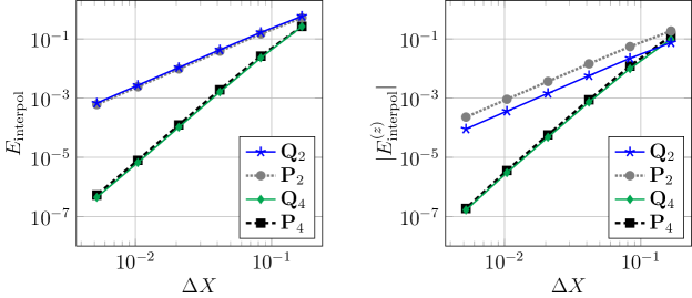
In order to get initial data satisfying the requirements, an approach based on polynomial interpolation is applied. We use p[n]​(x)superscript𝑝delimited-[]𝑛π‘₯p^{[n]}(x) to denote an interpolating polynomial of order n𝑛n, and let 𝐏[n]​(x)=[p1[n],p2[n],p3[n]]Tsubscript𝐏delimited-[]𝑛π‘₯superscriptsuperscriptsubscript𝑝1delimited-[]𝑛superscriptsubscript𝑝2delimited-[]𝑛superscriptsubscript𝑝3delimited-[]𝑛𝑇\mathbf{P}_{[n]}(x)=\left[p_{1}^{[n]},p_{2}^{[n]},p_{3}^{[n]}\right]^{T}, a vector containing an independent polynomial for each component in 𝐌𝐌\mathbf{M}, such that

𝐏[n]​(xi)=𝐌i,i=0,…,n.formulae-sequencesubscript𝐏delimited-[]𝑛subscriptπ‘₯𝑖subscriptπŒπ‘–π‘–0…𝑛\mathbf{P}_{[n]}(x_{i})=\mathbf{M}_{i},\quad i=0,\ldots,n.

When d>1𝑑1d>1, we apply one-dimensional interpolation in one space dimension after the other. For matters of simplicity, we regard a 1D problem in the following analytical error estimates. Due to the tensor product extension, the considerations generalize directly to higher dimensions.

Without loss of generality, we henceforth assume that we want to find initial data for the micro problem associated with the macro grid point at location xksubscriptπ‘₯π‘˜x_{k} based on 2​k2π‘˜2k-th order polynomial interpolation. This implies that the macro grid points involved in the process are xjsubscriptπ‘₯𝑗x_{j}, j=0,…,2​k𝑗0…2π‘˜j=0,...,2k.

According to standard theory, it holds for the interpolation errors that given 0≀i≀2​k0𝑖2π‘˜0\leq i\leq 2k and 𝐌∈C(2​k+1)​([x0,x2​k])𝐌superscript𝐢2π‘˜1subscriptπ‘₯0subscriptπ‘₯2π‘˜\mathbf{M}\in C^{(2k+1)}([x_{0},x_{2k}]),

supx∈[x0,x2​k]|𝐏[2​k](i)​(x)βˆ’πŒ(i)​(x,tj)|≀C​(Δ​X)2​k+1βˆ’i.subscriptsupremumπ‘₯subscriptπ‘₯0subscriptπ‘₯2π‘˜superscriptsubscript𝐏delimited-[]2π‘˜π‘–π‘₯superscriptπŒπ‘–π‘₯subscript𝑑𝑗𝐢superscriptΔ𝑋2π‘˜1𝑖\displaystyle\sup_{x\in[x_{0},x_{2k}]}|\mathbf{P}_{[2k]}^{(i)}(x)-\mathbf{M}^{(i)}(x,t_{j})|\leq C(\Delta X)^{2k+1-i}. (4.31)

Furthermore, it is well known that given a 2​k2π‘˜2k-th degree interpolating polynomial, it holds that

𝐏[2​k]′​(xk)=D[2​k]β€‹πŒβ€‹(xk,tj),𝐏[2​k]′′​(xk)=D[2​k]2β€‹πŒβ€‹(xk,tj),formulae-sequencesuperscriptsubscript𝐏delimited-[]2π‘˜β€²subscriptπ‘₯π‘˜subscript𝐷delimited-[]2π‘˜πŒsubscriptπ‘₯π‘˜subscript𝑑𝑗superscriptsubscript𝐏delimited-[]2π‘˜β€²β€²subscriptπ‘₯π‘˜superscriptsubscript𝐷delimited-[]2π‘˜2𝐌subscriptπ‘₯π‘˜subscript𝑑𝑗\displaystyle\mathbf{P}_{[2k]}^{\prime}(x_{k})=D_{[2k]}\mathbf{M}(x_{k},t_{j}),\qquad\mathbf{P}_{[2k]}^{\prime\prime}(x_{k})=D_{[2k]}^{2}\mathbf{M}({x_{k}},t_{j}),

where D[2​k]subscript𝐷delimited-[]2π‘˜D_{[2k]} and D[2​k]2subscriptsuperscript𝐷2delimited-[]2π‘˜D^{2}_{[2k]} denote the 2​k2π‘˜2k-th order standard central finite difference approximations to the first and second derivative, see for example [27]. As a direct consequence, we have in the grid point xksubscriptπ‘₯π‘˜x_{k},

|πŒβ€²β€‹(xk,tj)βˆ’π[2​k]′​(xk)|≀C​(Δ​X)2​k,|πŒβ€²β€²β€‹(xk,tj)βˆ’π[2​k]′′​(xk)|≀C​(Δ​X)2​k.formulae-sequencesuperscriptπŒβ€²subscriptπ‘₯π‘˜subscript𝑑𝑗superscriptsubscript𝐏delimited-[]2π‘˜β€²subscriptπ‘₯π‘˜πΆsuperscriptΔ𝑋2π‘˜superscriptπŒβ€²β€²subscriptπ‘₯π‘˜subscript𝑑𝑗superscriptsubscript𝐏delimited-[]2π‘˜β€²β€²subscriptπ‘₯π‘˜πΆsuperscriptΔ𝑋2π‘˜\displaystyle|\mathbf{M}^{\prime}(x_{k},t_{j})-\mathbf{P}_{[2k]}^{\prime}(x_{k})|\leq C(\Delta X)^{2k},\qquad|\mathbf{M}^{\prime\prime}(x_{k},t_{j})-\mathbf{P}_{[2k]}^{\prime\prime}(x_{k})|\leq C(\Delta X)^{2k}. (4.32)

Note that this gives a better bound for the error in the second derivative in the point xksubscriptπ‘₯π‘˜x_{k} than 4.31, valid on the whole interval [x0,x2​k]subscriptπ‘₯0subscriptπ‘₯2π‘˜[x_{0},x_{2k}]. The bounds in4.32 show that we have the required consistency, 4.30, between macro and micro derivatives when directly using 𝐏k​(x)subscriptππ‘˜π‘₯\mathbf{P}_{k}(x) to obtain the initial data for the micro problem. However, the disadvantage of this approach is that the polynomial vector 𝐏ksubscriptππ‘˜\mathbf{P}_{k} is not normalized. For the deviation of its length from one, it holds by 4.31 that

||𝐏[2​k]|βˆ’1|=||𝐏[2​k]|βˆ’|𝐌||≀|𝐏[2​k]βˆ’πŒ|≀C​(Δ​X)2​k+1.subscript𝐏delimited-[]2π‘˜1subscript𝐏delimited-[]2π‘˜πŒsubscript𝐏delimited-[]2π‘˜πŒπΆsuperscriptΔ𝑋2π‘˜1\left||\mathbf{P}_{[2k]}|-1\right|=\left||\mathbf{P}_{[2k]}|-|\mathbf{M}|\right|\leq|\mathbf{P}_{[2k]}-\mathbf{M}|\leq C(\Delta X)^{2k+1}.

Consider instead a normalized function π˜β€‹(x)𝐘π‘₯\mathbf{Y}(x) for which |π˜β€‹(x)|=1𝐘π‘₯1|\mathbf{Y}(x)|=1. Then the derivative π˜β€²superscriptπ˜β€²\mathbf{Y}^{\prime} is orthogonal to 𝐘𝐘\mathbf{Y} as it holds that

π˜β€²β€‹(x)β‹…π˜β€‹(x)=12​dd​x​|π˜β€‹(x)|2=0.β‹…superscriptπ˜β€²π‘₯𝐘π‘₯12𝑑𝑑π‘₯superscript𝐘π‘₯20\mathbf{Y}^{\prime}(x)\cdot\mathbf{Y}(x)=\frac{1}{2}\frac{d}{dx}|\mathbf{Y}(x)|^{2}=0.

In particular, this shows that πŒβ€²β‹…πŒ=0β‹…superscriptπŒβ€²πŒ0\mathbf{M}^{\prime}\cdot\mathbf{M}=0. However, in general,

πŒβ€‹(xk,tj)β‹…D[2​k]β€‹πŒβ€‹(xk,tj)=𝐏[2​k]​(xk)⋅𝐏[2​k]′​(xk)β‰ 0.β‹…πŒsubscriptπ‘₯π‘˜subscript𝑑𝑗subscript𝐷delimited-[]2π‘˜πŒsubscriptπ‘₯π‘˜subscript𝑑𝑗⋅subscript𝐏delimited-[]2π‘˜subscriptπ‘₯π‘˜superscriptsubscript𝐏delimited-[]2π‘˜β€²subscriptπ‘₯π‘˜0\mathbf{M}(x_{k},t_{j})\cdot D_{[2k]}\mathbf{M}(x_{k},t_{j})=\mathbf{P}_{[2k]}(x_{k})\cdot\mathbf{P}_{[2k]}^{\prime}(x_{k})\neq 0.

Hence there is no normalized interpolating function 𝐘𝐘\mathbf{Y} such that π˜β€²β€‹(xk)superscriptπ˜β€²subscriptπ‘₯k\mathbf{Y}^{\prime}(x_{\mathrm{k}}) becomes a standard linear 2​k2π‘˜2k-th order central difference approximation, D[2​k]subscript𝐷delimited-[]2π‘˜D_{[2k]}. In the following, we consider the normalized interpolating function 𝐐[n]​(x)subscript𝐐delimited-[]𝑛π‘₯\mathbf{Q}_{[n]}(x) defined as

𝐐[n]​(x):=𝐏[n]​(x)/|𝐏[n]​(x)|,assignsubscript𝐐delimited-[]𝑛π‘₯subscript𝐏delimited-[]𝑛π‘₯subscript𝐏delimited-[]𝑛π‘₯\mathbf{Q}_{[n]}(x):=\mathbf{P}_{[n]}(x)/|\mathbf{P}_{[n]}(x)|\,, (4.33)

and show that it satisfies the consistency requirement 4.30.

Lemma 4.1.

In one space dimension, the normalized function 𝐐[2​k]subscript𝐐delimited-[]2π‘˜\mathbf{Q}_{[2k]} satisfies 4.30 with β„“=2​kβ„“2π‘˜\ell=2k.

Proof 4.2.

As |𝐏[2​k]​(xi)|=|𝐌i|=1subscript𝐏delimited-[]2π‘˜subscriptπ‘₯𝑖subscriptπŒπ‘–1|\mathbf{P}_{[2k]}(x_{i})|=|\mathbf{M}_{i}|=1 in the grid points xisubscriptπ‘₯𝑖x_{i}, where i=0,…,2​k𝑖0…2π‘˜i=0,...,2k, it follows directly that 𝐐[2​k]​(xi)=𝐌isubscript𝐐delimited-[]2π‘˜subscriptπ‘₯𝑖subscriptπŒπ‘–\mathbf{Q}_{[2k]}(x_{i})=\mathbf{M}_{i} for i=0,…,2​k𝑖0…2π‘˜i=0,...,2k, the normalized function still interpolates the given points.

For the first derivative of 𝐐[2​k]subscript𝐐delimited-[]2π‘˜\mathbf{Q}_{[2k]}, it holds that

𝐐[2​k]β€²=dd​x​(𝐏[2​k]/|𝐏[2​k]|)=𝐏[2​k]β€²/|𝐏[2​k]|βˆ’(𝐏[2​k]T​𝐏[2​k]β€²)​𝐏[2​k]/|𝐏[2​k]|3,superscriptsubscript𝐐delimited-[]2π‘˜β€²π‘‘π‘‘π‘₯subscript𝐏delimited-[]2π‘˜subscript𝐏delimited-[]2π‘˜superscriptsubscript𝐏delimited-[]2π‘˜β€²subscript𝐏delimited-[]2π‘˜superscriptsubscript𝐏delimited-[]2π‘˜π‘‡superscriptsubscript𝐏delimited-[]2π‘˜β€²subscript𝐏delimited-[]2π‘˜superscriptsubscript𝐏delimited-[]2π‘˜3\begin{split}\mathbf{Q}_{[2k]}^{\prime}&=\frac{d}{dx}\left(\mathbf{P}_{[2k]}/|\mathbf{P}_{[2k]}|\right)=\mathbf{P}_{[2k]}^{\prime}/|\mathbf{P}_{[2k]}|-(\mathbf{P}_{[2k]}^{T}\mathbf{P}_{[2k]}^{\prime})\mathbf{P}_{[2k]}/|\mathbf{P}_{[2k]}|^{3}\,,\end{split}

which, together with the fact that 𝐏[2​k]​(xi)=𝐌isubscript𝐏delimited-[]2π‘˜subscriptπ‘₯𝑖subscriptπŒπ‘–\mathbf{P}_{[2k]}(x_{i})=\mathbf{M}_{i} for i=0,..,2ki=0,..,2k, implies that

𝐐[2​k]′​(xi)=(πˆβˆ’πŒiβ€‹πŒiT)​𝐏[2​k]′​(xi).superscriptsubscript𝐐delimited-[]2π‘˜β€²subscriptπ‘₯π‘–πˆsubscriptπŒπ‘–superscriptsubscriptπŒπ‘–π‘‡superscriptsubscript𝐏delimited-[]2π‘˜β€²subscriptπ‘₯𝑖\mathbf{Q}_{[2k]}^{\prime}(x_{i})=(\mathbf{I}-\mathbf{M}_{i}\mathbf{M}_{i}^{T})\mathbf{P}_{[2k]}^{\prime}(x_{i}). (4.34)

In particular, it holds due to orthogonality that

|𝐐[2​k]′​(xi)βˆ’πŒβ€²β€‹(xi)|superscriptsubscript𝐐delimited-[]2π‘˜β€²subscriptπ‘₯𝑖superscriptπŒβ€²subscriptπ‘₯𝑖\displaystyle\left|\mathbf{Q}_{[2k]}^{\prime}(x_{i})-\mathbf{M}^{\prime}(x_{i})\right| =|(πˆβˆ’πŒiβ€‹πŒiT)​(𝐏[2​k]′​(xi)βˆ’πŒβ€²β€‹(xi))|absent𝐈subscriptπŒπ‘–superscriptsubscriptπŒπ‘–π‘‡superscriptsubscript𝐏delimited-[]2π‘˜β€²subscriptπ‘₯𝑖superscriptπŒβ€²subscriptπ‘₯𝑖\displaystyle=\left|(\mathbf{I}-\mathbf{M}_{i}\mathbf{M}_{i}^{T})\left(\mathbf{P}_{[2k]}^{\prime}(x_{i})-\mathbf{M}^{\prime}(x_{i})\right)\right|
≀C​|𝐏[2​k]′​(xi)βˆ’πŒβ€²β€‹(xi)|≀C​(Δ​X)2​k,absent𝐢superscriptsubscript𝐏delimited-[]2π‘˜β€²subscriptπ‘₯𝑖superscriptπŒβ€²subscriptπ‘₯𝑖𝐢superscriptΔ𝑋2π‘˜\displaystyle\leq C|\mathbf{P}_{[2k]}^{\prime}(x_{i})-\mathbf{M}^{\prime}(x_{i})|\leq C(\Delta X)^{2k},

hence 𝐐[2​k]′​(xk)superscriptsubscript𝐐delimited-[]2π‘˜β€²subscriptπ‘₯π‘˜\mathbf{Q}_{[2k]}^{\prime}(x_{k}) is a 2​k2π‘˜2k-th order approximation to the derivative of 𝐌𝐌\mathbf{M} in xksubscriptπ‘₯π‘˜x_{k}. For the second derivative of 𝐐[n]subscript𝐐delimited-[]𝑛\mathbf{Q}_{[n]}, it holds in general that

𝐐[n]β€²β€²=𝐏[n]β€²β€²|𝐏[n]|βˆ’2​(𝐏[n]⋅𝐏[n]β€²)​𝐏[n]β€²|𝐏[n]|3+3​(𝐏[n]⋅𝐏[n]β€²)2​𝐏[n]|𝐏[n]|5βˆ’(|𝐏[n]β€²|2+𝐏[n]′′⋅𝐏[n])​𝐏[n]|𝐏[n]|3,superscriptsubscript𝐐delimited-[]𝑛′′superscriptsubscript𝐏delimited-[]𝑛′′subscript𝐏delimited-[]𝑛2β‹…subscript𝐏delimited-[]𝑛superscriptsubscript𝐏delimited-[]𝑛′superscriptsubscript𝐏delimited-[]𝑛′superscriptsubscript𝐏delimited-[]𝑛33superscriptβ‹…subscript𝐏delimited-[]𝑛superscriptsubscript𝐏delimited-[]𝑛′2subscript𝐏delimited-[]𝑛superscriptsubscript𝐏delimited-[]𝑛5superscriptsuperscriptsubscript𝐏delimited-[]𝑛′2β‹…superscriptsubscript𝐏delimited-[]𝑛′′subscript𝐏delimited-[]𝑛subscript𝐏delimited-[]𝑛superscriptsubscript𝐏delimited-[]𝑛3\mathbf{Q}_{[n]}^{\prime\prime}=\frac{\mathbf{P}_{[n]}^{\prime\prime}}{|\mathbf{P}_{[n]}|}-2\frac{(\mathbf{P}_{[n]}\cdot\mathbf{P}_{[n]}^{\prime})\mathbf{P}_{[n]}^{\prime}}{|\mathbf{P}_{[n]}|^{3}}+3\frac{(\mathbf{P}_{[n]}\cdot\mathbf{P}_{[n]}^{\prime})^{2}\mathbf{P}_{[n]}}{|\mathbf{P}_{[n]}|^{5}}-\frac{(|\mathbf{P}_{[n]}^{\prime}|^{2}+\mathbf{P}_{[n]}^{\prime\prime}\cdot\mathbf{P}_{[n]})\mathbf{P}_{[n]}}{|\mathbf{P}_{[n]}|^{3}}, (4.35)

where we can rewrite

|𝐏[n]β€²|2+𝐏[n]′′⋅𝐏[n]=(𝐏[n]βˆ’πŒ)⋅𝐏[n]β€²β€²+(𝐏[n]β€²βˆ’πŒβ€²)β‹…(πŒβ€²+𝐏[n]β€²)+(𝐏[n]β€²β€²βˆ’πŒβ€²β€²)β‹…πŒ,superscriptsuperscriptsubscript𝐏delimited-[]𝑛′2β‹…superscriptsubscript𝐏delimited-[]𝑛′′subscript𝐏delimited-[]𝑛⋅subscript𝐏delimited-[]π‘›πŒsuperscriptsubscript𝐏delimited-[]𝑛′′⋅superscriptsubscript𝐏delimited-[]𝑛′superscriptπŒβ€²superscriptπŒβ€²superscriptsubscript𝐏delimited-[]𝑛′⋅superscriptsubscript𝐏delimited-[]𝑛′′superscriptπŒβ€²β€²πŒ|\mathbf{P}_{[n]}^{\prime}|^{2}+\mathbf{P}_{[n]}^{\prime\prime}\cdot\mathbf{P}_{[n]}=(\mathbf{P}_{[n]}-\mathbf{M})\cdot\mathbf{P}_{[n]}^{\prime\prime}+(\mathbf{P}_{[n]}^{\prime}-\mathbf{M}^{\prime})\cdot(\mathbf{M}^{\prime}+\mathbf{P}_{[n]}^{\prime})+(\mathbf{P}_{[n]}^{\prime\prime}-\mathbf{M}^{\prime\prime})\cdot\mathbf{M},

For a 2​k2π‘˜2k-th order interpolating polynomial, we hence have in the grid point xksubscriptπ‘₯π‘˜x_{k} that

|(|𝐏[2​k]′​(xk)|2+𝐏[2​k]′′​(xk)⋅𝐏[2​k]​(xk))​𝐏2​k​(xk)|superscriptsuperscriptsubscript𝐏delimited-[]2π‘˜β€²subscriptπ‘₯π‘˜2β‹…superscriptsubscript𝐏delimited-[]2π‘˜β€²β€²subscriptπ‘₯π‘˜subscript𝐏delimited-[]2π‘˜subscriptπ‘₯π‘˜subscript𝐏2π‘˜subscriptπ‘₯π‘˜\displaystyle\left|\left(|\mathbf{P}_{[2k]}^{\prime}(x_{k})|^{2}+\mathbf{P}_{[2k]}^{\prime\prime}(x_{k})\cdot\mathbf{P}_{[2k]}(x_{k})\right)\mathbf{P}_{2k}(x_{k})\right|
≀|(𝐏[2​k]′​(xk)βˆ’πŒβ€²β€‹(xk))β‹…(πŒβ€²β€‹(xk)+𝐏[2​k]′​(xk))+(𝐏[2​k]′′​(xk)βˆ’πŒβ€²β€²β€‹(xk))β‹…πŒβ€‹(xk)|absentβ‹…superscriptsubscript𝐏delimited-[]2π‘˜β€²subscriptπ‘₯π‘˜superscriptπŒβ€²subscriptπ‘₯π‘˜superscriptπŒβ€²subscriptπ‘₯π‘˜superscriptsubscript𝐏delimited-[]2π‘˜β€²subscriptπ‘₯π‘˜β‹…superscriptsubscript𝐏delimited-[]2π‘˜β€²β€²subscriptπ‘₯π‘˜superscriptπŒβ€²β€²subscriptπ‘₯π‘˜πŒsubscriptπ‘₯π‘˜\displaystyle\hskip 28.45274pt\leq\left|(\mathbf{P}_{[2k]}^{\prime}(x_{k})-\mathbf{M}^{\prime}(x_{k}))\cdot(\mathbf{M}^{\prime}(x_{k})+\mathbf{P}_{[2k]}^{\prime}(x_{k}))+(\mathbf{P}_{[2k]}^{\prime\prime}(x_{k})-\mathbf{M}^{\prime\prime}(x_{k}))\cdot\mathbf{M}(x_{k})\right|
≀C(|(𝐏[2​k]β€²(xk)βˆ’πŒβ€²(xk))|+|𝐏[2​k]β€²β€²(xk)βˆ’πŒβ€²β€²(xk))|)≀C(Ξ”X)2​k,\displaystyle\hskip 28.45274pt\leq C\left(\left|(\mathbf{P}_{[2k]}^{\prime}(x_{k})-\mathbf{M}^{\prime}(x_{k}))\right|+\left|\mathbf{P}_{[2k]}^{\prime\prime}(x_{k})-\mathbf{M}^{\prime\prime}(x_{k}))\right|\right)\leq C(\Delta X)^{2k},

where we used 4.32 in the last step. Moreover, it holds due to orthogonality and 4.32 that

|𝐏[2​k]​(xk)⋅𝐏[2​k]′​(xk)|=|𝐌kβ‹…(𝐏[2​k]′​(xk)βˆ’πŒβ€²β€‹(xk))|≀|𝐏[2​k]′​(xk)βˆ’πŒβ€²β€‹(xk)|≀C​(Δ​X)2​k.β‹…subscript𝐏delimited-[]2π‘˜subscriptπ‘₯π‘˜superscriptsubscript𝐏delimited-[]2π‘˜β€²subscriptπ‘₯π‘˜β‹…subscriptπŒπ‘˜superscriptsubscript𝐏delimited-[]2π‘˜β€²subscriptπ‘₯π‘˜superscriptπŒβ€²subscriptπ‘₯π‘˜superscriptsubscript𝐏delimited-[]2π‘˜β€²subscriptπ‘₯π‘˜superscriptπŒβ€²subscriptπ‘₯π‘˜πΆsuperscriptΔ𝑋2π‘˜|\mathbf{P}_{[2k]}(x_{k})\cdot\mathbf{P}_{[2k]}^{\prime}(x_{k})|=|\mathbf{M}_{k}\cdot(\mathbf{P}_{[2k]}^{\prime}(x_{k})-\mathbf{M}^{\prime}(x_{k}))|\leq|\mathbf{P}_{[2k]}^{\prime}(x_{k})-\mathbf{M}^{\prime}(x_{k})|\leq C(\Delta X)^{2k}.

It therefore follows that

|𝐐[2​k]′′​(xk)βˆ’π[2​k]′′​(xk)|superscriptsubscript𝐐delimited-[]2π‘˜β€²β€²subscriptπ‘₯π‘˜superscriptsubscript𝐏delimited-[]2π‘˜β€²β€²subscriptπ‘₯π‘˜\displaystyle|\mathbf{Q}_{[2k]}^{\prime\prime}(x_{k})-\mathbf{P}_{[2k]}^{\prime\prime}(x_{k})| ≀2​|(𝐏[2​k]​(xk)⋅𝐏[2​k]′​(xk))​𝐏[2​k]′​(xk)|absent2β‹…subscript𝐏delimited-[]2π‘˜subscriptπ‘₯π‘˜superscriptsubscript𝐏delimited-[]2π‘˜β€²subscriptπ‘₯π‘˜superscriptsubscript𝐏delimited-[]2π‘˜β€²subscriptπ‘₯π‘˜\displaystyle\leq 2\left|(\mathbf{P}_{[2k]}(x_{k})\cdot\mathbf{P}_{[2k]}^{\prime}(x_{k}))\mathbf{P}_{[2k]}^{\prime}(x_{k})\right|
+3​|(𝐏[2​k]​(xk)⋅𝐏[2​k]′​(xk))2​𝐏[2​k]​(xk)|3superscriptβ‹…subscript𝐏delimited-[]2π‘˜subscriptπ‘₯π‘˜superscriptsubscript𝐏delimited-[]2π‘˜β€²subscriptπ‘₯π‘˜2subscript𝐏delimited-[]2π‘˜subscriptπ‘₯π‘˜\displaystyle+3\left|\left(\mathbf{P}_{[2k]}(x_{k})\cdot\mathbf{P}_{[2k]}^{\prime}(x_{k})\right)^{2}\mathbf{P}_{[2k]}(x_{k})\right|
+|(|𝐏[2​k]′​(xk)|2+𝐏[2​k]′′​(xk)⋅𝐏[2​k]​(xk))​𝐏2​k​(xk)|≀C​(Δ​X)2​k,superscriptsuperscriptsubscript𝐏delimited-[]2π‘˜β€²subscriptπ‘₯π‘˜2β‹…superscriptsubscript𝐏delimited-[]2π‘˜β€²β€²subscriptπ‘₯π‘˜subscript𝐏delimited-[]2π‘˜subscriptπ‘₯π‘˜subscript𝐏2π‘˜subscriptπ‘₯π‘˜πΆsuperscriptΔ𝑋2π‘˜\displaystyle+\left|\left(|\mathbf{P}_{[2k]}^{\prime}(x_{k})|^{2}+\mathbf{P}_{[2k]}^{\prime\prime}(x_{k})\cdot\mathbf{P}_{[2k]}(x_{k})\right)\mathbf{P}_{2k}(x_{k})\right|\leq C(\Delta X)^{2k},

which by 4.32 implies that 𝐐k′′​(xk)superscriptsubscriptππ‘˜β€²β€²subscriptπ‘₯π‘˜\mathbf{Q}_{k}^{\prime\prime}(x_{k}) is a 2​k2π‘˜2k-th order approximation to πŒβ€²β€²superscriptπŒβ€²β€²\mathbf{M}^{\prime\prime} (but not a standard linear central finite difference approximation).

We can conclude that when using either 𝐏[2​k]subscript𝐏delimited-[]2π‘˜\mathbf{P}_{[2k]} or 𝐐[2​k]subscript𝐐delimited-[]2π‘˜\mathbf{Q}_{[2k]} to obtain initial data 𝐦initsubscript𝐦init\mathbf{m}_{\mathrm{init}} for the HMM micro problem, then βˆ‚x​x𝐦init​(0)subscriptπ‘₯π‘₯subscript𝐦init0\partial_{xx}\mathbf{m}_{\mathrm{init}}(0) is a 2​k2π‘˜2k-th order approximation to βˆ‚x​xπŒβ€‹(xk,tj)subscriptπ‘₯π‘₯𝐌subscriptπ‘₯π‘˜subscript𝑑𝑗\partial_{xx}\mathbf{M}(x_{k},t_{j}), where xksubscriptπ‘₯π‘˜x_{k} is the grid point in the middle of the interpolation stencil. Similarly, in two space dimensions, βˆ‚x​y𝐦init​(0)subscriptπ‘₯𝑦subscript𝐦init0\partial_{xy}\mathbf{m}_{\mathrm{init}}(0) and βˆ‚y​y𝐦init​(0)subscript𝑦𝑦subscript𝐦init0\partial_{yy}\mathbf{m}_{\mathrm{init}}(0) are 2​k2π‘˜2k-th order approximations to βˆ‚x​yπŒβ€‹(xk,tj)subscriptπ‘₯π‘¦πŒsubscriptπ‘₯π‘˜subscript𝑑𝑗\partial_{xy}\mathbf{M}(x_{k},t_{j}) and βˆ‚y​yπŒβ€‹(xk,tj)subscriptπ‘¦π‘¦πŒsubscriptπ‘₯π‘˜subscript𝑑𝑗\partial_{yy}\mathbf{M}(x_{k},t_{j}). Thus, the discretization error, which corresponds to the interpolation error, is

Edisc=βˆ‡β‹…(βˆ‡π¦init​(0)​𝐀H)βˆ’βˆ‡β‹…(βˆ‡πŒβ€‹(xk,tj)​𝐀H)=C​(Δ​X)2​k.subscript𝐸discβ‹…bold-βˆ‡bold-βˆ‡subscript𝐦init0superscript𝐀𝐻⋅bold-βˆ‡bold-βˆ‡πŒsubscriptπ‘₯π‘˜subscript𝑑𝑗superscript𝐀𝐻𝐢superscriptΔ𝑋2π‘˜\displaystyle E_{\mathrm{disc}}=\boldsymbol{\nabla}\cdot(\boldsymbol{\nabla}\mathbf{m}_{\mathrm{init}}(0)\mathbf{A}^{H})-\boldsymbol{\nabla}\cdot(\boldsymbol{\nabla}\mathbf{M}(x_{k},t_{j})\mathbf{A}^{H})=C(\Delta X)^{2k}. (4.36)

Both 𝐏[2​k]subscript𝐏delimited-[]2π‘˜\mathbf{P}_{[2k]} and 𝐐[2​k]subscript𝐐delimited-[]2π‘˜\mathbf{Q}_{[2k]} hence satisfy the consistency requirement 4.30 for the initial data. However, only 𝐐[2​k]subscript𝐐delimited-[]2π‘˜\mathbf{Q}_{[2k]} is normalized, therefore this is what we choose subsequently. Typically, the difference between the approximations is only rather small, though, as shown in the following numerical example.

Numerical example

As an example, consider the initial data for a micro problem on a 2D domain of size 10​Ρ10πœ€10\varepsilon in each space dimension, obtained by interpolation from the macro initial data of (EX2) and (EX3).

We first investigate the maximal deviation of the length of 𝐦initsubscript𝐦init\mathbf{m}_{\mathrm{init}} from one when using 𝐏[2]subscript𝐏delimited-[]2\mathbf{P}_{[2]} and 𝐏[4]subscript𝐏delimited-[]4\mathbf{P}_{[4]} to obtain the initial data. In FigureΒ 8, this error is shown for varying Δ​XΔ𝑋\Delta X and different values of Ξ΅πœ€\varepsilon.

Refer to caption
Figure 8: Maximum norm deviation in polynomial interpolation initial data 𝐏[2]subscript𝐏delimited-[]2\mathbf{P}_{[2]} (left) and 𝐏[4]subscript𝐏delimited-[]4\mathbf{P}_{[4]} (right) from one given a micro domain size of 10​Ρ10πœ€10\varepsilon, for several values of Ξ΅πœ€\varepsilon. 2D problem with macro initial data as in (EX3) and (EX2). Only values where 2​k​Δ​X>10​Ρ2π‘˜Ξ”π‘‹10πœ€2k\Delta X>10\varepsilon are plotted to avoid extrapolation.

One can observe that the deviation decreases as the macro step size Δ​XΔ𝑋\Delta X decreases. Moreover, especially for high Δ​XΔ𝑋\Delta X values, smaller Ξ΅πœ€\varepsilon result in smaller deviations. This is due to the fact that a smaller Ξ΅πœ€\varepsilon corresponds to a smaller micro domain, around xksubscriptπ‘₯π‘˜x_{k}. The maximum possible norm deviation is only attained further away from xksubscriptπ‘₯π‘˜x_{k}. In the limit, as Ξ΅β†’0β†’πœ€0\varepsilon\to 0, the norm deviation vanishes.

Next, we examine the difference between 𝐏[2​k]subscript𝐏delimited-[]2π‘˜\mathbf{P}_{[2k]} and 𝐐[2​k]subscript𝐐delimited-[]2π‘˜\mathbf{Q}_{[2k]} and the order of accuracy of the resulting approximations to βˆ‡β‹…(βˆ‡πŒπ€H)β‹…bold-βˆ‡bold-βˆ‡superscriptπŒπ€π»\boldsymbol{\nabla}\cdot(\boldsymbol{\nabla}\mathbf{M}\mathbf{A}^{H}). In the left subplot in FigureΒ 9, the error Ediscsubscript𝐸discE_{\mathrm{disc}} is shown for several values of Δ​XΔ𝑋\Delta X and for second and fourth order interpolation. The expected convergence rates of (Δ​X)2​ksuperscriptΔ𝑋2π‘˜(\Delta X)^{2k} can be observed for both approximations, based on 𝐏[2​k]subscript𝐏delimited-[]2k\mathbf{P}_{\mathrm{[2k]}} and 𝐐[2​k]subscript𝐐delimited-[]2k\mathbf{Q}_{\mathrm{[2k]}}.

Refer to caption
Figure 9: Interpolation error Ediscsubscript𝐸discE_{\mathrm{disc}} with and without normalization, i.e. using 𝐐[2​k]subscript𝐐delimited-[]2π‘˜\mathbf{Q}_{[2k]} and 𝐏[2​k]subscript𝐏delimited-[]2π‘˜\mathbf{P}_{[2k]}, when varying macro grid spacing Δ​XΔ𝑋\Delta X. 222nd and 444th order interpolation. Left: norm of the error between approximated and actual effective field for (EX2). Right: z𝑧z-component only.

In the right subplot, only the difference between the z𝑧z-components of βˆ‡β‹…(βˆ‡π¦init​𝐀H)β‹…bold-βˆ‡bold-βˆ‡subscript𝐦initsuperscript𝐀𝐻\boldsymbol{\nabla}\cdot(\boldsymbol{\nabla}\mathbf{m}_{\mathrm{init}}\mathbf{A}^{H}) and βˆ‡β‹…(βˆ‡πŒπ€H)β‹…bold-βˆ‡bold-βˆ‡superscriptπŒπ€π»\boldsymbol{\nabla}\cdot(\boldsymbol{\nabla}\mathbf{M}\mathbf{A}^{H}) is considered to emphasize the fact that while 𝐏[2​k]subscript𝐏delimited-[]2π‘˜\mathbf{P}_{[2k]} and 𝐐[2​k]subscript𝐐delimited-[]2π‘˜\mathbf{Q}_{[2k]} result in approximations of the same order of accuracy, they do not give the same approximation.

4.2 Boundary conditions

In this section, the issue of boundary conditions for the HMM micro problem is discussed. In the case of a periodic material coefficient, as considered for the estimate in TheoremΒ 2.3, the micro problem would ideally be solved on the whole domain ΩΩ\Omega with periodic boundary conditions, even though the resulting solution is only averaged over a small domain [βˆ’ΞΌ,ΞΌ]dsuperscriptπœ‡πœ‡π‘‘[-\mu,\mu]^{d}. This is not a reasonable choice in practice, since the related computational cost is too high. We therefore have to restrict the size of the computational domain for the micro problem and complete it with boundary conditions. Every choice of boundary conditions introduces some error inside the domain in comparison to the whole domain solution since it is not possible to exactly match both β€œincoming” and β€œoutgoing” dynamics. In FigureΒ 10, the effect of boundary conditions in comparison to the solution on a much larger domain is illustrated for one example 1D microproblem with the setup (EX1). The solution in the micro domain as well as the errors due to two kinds of boundary conditions are plotted: assuming periodicity of π¦Ξ΅βˆ’π¦initsuperscriptπ¦πœ€subscript𝐦init\mathbf{m}^{\varepsilon}-\mathbf{m}_{\mathrm{init}} (middle) and homogeneous Dirichlet boundary conditions for π¦Ξ΅βˆ’π¦initsuperscriptπ¦πœ€subscript𝐦init\mathbf{m}^{\varepsilon}-\mathbf{m}_{\mathrm{init}} (right).

Refer to caption
Refer to caption
Refer to caption
Figure 10: Example (EX1) with Ξ±=0.01𝛼0.01\alpha=0.01, comparison of solution on micro domain [βˆ’ΞΌβ€²,ΞΌβ€²]superscriptπœ‡β€²superscriptπœ‡β€²[-\mu^{\prime},\mu^{\prime}], where ΞΌβ€²=5​Ρsuperscriptπœ‡β€²5πœ€\mu^{\prime}=5\varepsilon and Ξ΅=2β‹…10βˆ’3πœ€β‹…2superscript103\varepsilon=2\cdot 10^{-3}, to solution on a 10 times larger domain. Left: x component of the expected solution, middle: error with periodic boundary conditions for π¦Ξ΅βˆ’π¦initsuperscriptπ¦πœ€subscript𝐦init\mathbf{m}^{\varepsilon}-\mathbf{m}_{\mathrm{init}}, right: error with Dirichlet boundary condition.

In both cases, one can observe errors propagating into the domain from both boundaries as time increases, even though the amplitude of the errors is influenced by the type of condition. Since we cannot remove this problem even when considering more involved boundary conditions, we choose to solve the micro problem on a domain [βˆ’ΞΌβ€²,ΞΌβ€²]dsuperscriptsuperscriptπœ‡β€²superscriptπœ‡β€²π‘‘[-\mu^{\prime},\mu^{\prime}]^{d}, for some ΞΌβ€²β‰₯ΞΌsuperscriptπœ‡β€²πœ‡\mu^{\prime}\geq\mu, with Dirichlet boundary conditions and only average over [βˆ’ΞΌ,ΞΌ]dsuperscriptπœ‡πœ‡π‘‘[-\mu,\mu]^{d}. The size of the domain extension ΞΌβ€²βˆ’ΞΌsuperscriptπœ‡β€²πœ‡\mu^{\prime}-\mu together with the time parameter Ξ·πœ‚\eta determine how large the boundary error EΞΌβ€²subscript𝐸superscriptπœ‡β€²E_{\mu^{\prime}} in 4.29 becomes. For larger values of Ξ·πœ‚\eta, we expect a larger ΞΌβ€²βˆ’ΞΌsuperscriptπœ‡β€²πœ‡\mu^{\prime}-\mu to be required to obtain EΞΌsubscriptπΈπœ‡E_{\mu} below a given threshold, since given a longer final time the errors can propagate further into the domain. This is investigated in more detail in the next section.

4.3 Size of micro domain

Here, we investigate how to choose the size of the micro problem domain. There are three important parameters that have to be set, ΞΌπœ‡\mu and Ξ·πœ‚\eta as in TheoremΒ 2.3, which determine the size of the averaging domain in space and time, as well as the outer box size ΞΌβ€²superscriptπœ‡β€²\mu^{\prime}. Note that the optimal choice of all three parameters is dependent on the given initial data and the material coefficient.

To determine the influence of the respective parameters, we consider the example (EX2), with a periodic material coefficient, and investigate for one micro problem the error Eavgsubscript𝐸avgE_{\mathrm{avg}} as given in 4.29. Throughout this section, we consider averaging kernels K,K0𝐾superscript𝐾0K,K^{0} with px=pt=3subscript𝑝π‘₯subscript𝑝𝑑3p_{x}=p_{t}=3 and qx=qt=7subscriptπ‘žπ‘₯subscriptπ‘žπ‘‘7q_{x}=q_{t}=7, based on the experiments in [22]. Typically, Ξ΅=1/400πœ€1400\varepsilon=1/400 is used, which results a value of EΞ΅subscriptπΈπœ€E_{\varepsilon} that is relatively low compared to other contributions to Eavgsubscript𝐸avgE_{\mathrm{avg}}.

Averaging domain size, ΞΌπœ‡\mu

To begin with, we choose a large value for the computational domain ΞΌβ€²superscriptπœ‡β€²\mu^{\prime}, so that

Eavgβ‰ˆEΞ΅+EΞ·+EΞΌ.subscript𝐸avgsubscriptπΈπœ€subscriptπΈπœ‚subscriptπΈπœ‡E_{\mathrm{avg}}\approx E_{\varepsilon}+E_{\eta}+E_{\mu}.

We then vary the averaging parameter ΞΌπœ‡\mu, which affects the error contribution EΞΌsubscriptπΈπœ‡E_{\mu}, that satisfies 2.13, repeated here for convenience,

Eμ≀C​(ΞΌpx+1+(Ρμ)qx+2).subscriptπΈπœ‡πΆsuperscriptπœ‡subscript𝑝π‘₯1superscriptπœ€πœ‡subscriptπ‘žπ‘₯2E_{\mu}\leq C\left(\mu^{p_{x}+1}+\left(\frac{\varepsilon}{\mu}\right)^{q_{x}+2}\right). (4.37)

Based on the considerations in [22] and TheoremΒ 2.3, we expect that ΞΌπœ‡\mu should be chosen to be a multiple of Ξ΅πœ€\varepsilon, which is the scale of the fast spatial oscillations in the problem. With the given averaging kernel, the first term on the right-hand side in 4.37 then is small in comparison to the other error contributions and the second term dominates EΞΌsubscriptπΈπœ‡E_{\mu}.

In FigureΒ 11, the development of Eavgsubscript𝐸avgE_{\mathrm{avg}} when increasing ΞΌπœ‡\mu for (EX2) is shown for several values of Ξ·πœ‚\eta and α𝛼\alpha. One can observe that as ΞΌπœ‡\mu is increased, the error decreases rapidly from high initial levels. This is due to the contribution C​(Ρμ)qx+2𝐢superscriptπœ€πœ‡subscriptπ‘žπ‘₯2C\left(\frac{\varepsilon}{\mu}\right)^{q_{x}+2} to EΞΌsubscriptπΈπœ‡E_{\mu}. Once ΞΌπœ‡\mu becomes sufficiently large, in this example around ΞΌβ‰ˆ3.5β€‹Ξ΅πœ‡3.5πœ€\mu\approx 3.5\varepsilon, the error does not change significantly anymore but stays at a constant level, depending on Ξ·πœ‚\eta and α𝛼\alpha. Here EΞΌsubscriptπΈπœ‡E_{\mu} no longer dominates the error, which will instead be determined by EΞ·subscriptπΈπœ‚E_{\eta} and EΞ΅subscriptπΈπœ€E_{\varepsilon}. One can observe that longer times Ξ·πœ‚\eta result in lower overall errors. Furthermore, the errors in the high damping case, Ξ±=1𝛼1\alpha=1, are considerably lower than with Ξ±=0.1𝛼0.1\alpha=0.1 or Ξ±=0.01𝛼0.01\alpha=0.01. However, note that the required value of ΞΌπœ‡\mu until the errors no longer decrease is independent of both α𝛼\alpha and Ξ·πœ‚\eta. In the subsequent investigations, we therefore choose a fixed value of ΞΌπœ‡\mu which is slightly above this number, thus making sure that EΞΌsubscriptπΈπœ‡E_{\mu} does not significantly influence the overall error observed there.

Refer to caption
Figure 11: (EX2): Influence of spatial averaging size ΞΌπœ‡\mu on the overall error in one micro problem for several values of Ξ·πœ‚\eta and α𝛼\alpha when Ξ΅=1/400πœ€1400\varepsilon=1/400. Kernel parameters px=pt=3subscript𝑝π‘₯subscript𝑝𝑑3p_{x}=p_{t}=3 and qx=qt=7subscriptπ‘žπ‘₯subscriptπ‘žπ‘‘7q_{x}=q_{t}=7. The outer box size ΞΌβ€²superscriptπœ‡β€²\mu^{\prime} is chosen sufficiently large to not significantly influence the results.

Full domain size, ΞΌβ€²superscriptπœ‡β€²\mu^{\prime}

Next, we study the effect of the size of the computational domain, which is determined by ΞΌβ€²superscriptπœ‡β€²\mu^{\prime}, on the error Eavgsubscript𝐸avgE_{\mathrm{avg}}. We here choose ΞΌπœ‡\mu large enough so that

Eavgβ‰ˆEΞ΅+EΞ·+EΞΌβ€².subscript𝐸avgsubscriptπΈπœ€subscriptπΈπœ‚subscript𝐸superscriptπœ‡β€²E_{\mathrm{avg}}\approx E_{\varepsilon}+E_{\eta}+E_{\mu^{\prime}}.

We consider the same choices of α𝛼\alpha and Ξ·πœ‚\eta-values as in the previous example, and vary ΞΌβ€²superscriptπœ‡β€²\mu^{\prime} to investigate EΞΌβ€²subscript𝐸superscriptπœ‡β€²E_{\mu^{\prime}}. Note that in contrast to the other error terms, we do not have a model for EΞΌβ€²subscript𝐸superscriptπœ‡β€²E_{\mu^{\prime}}. As shown in FigureΒ 12, a value of ΞΌβ€²superscriptπœ‡β€²\mu^{\prime} that is only slightly larger than ΞΌπœ‡\mu gives a high error, which decreases as ΞΌβ€²superscriptπœ‡β€²\mu^{\prime} is increased, until the same error levels as in FigureΒ 11, determined by EΞ·subscriptπΈπœ‚E_{\eta} and EΞ΅subscriptπΈπœ€E_{\varepsilon}, are reached.

Refer to caption
Figure 12: (EX2): Influence of the extension of the computational domain, [βˆ’ΞΌβ€²,ΞΌβ€²]dsuperscriptsuperscriptπœ‡β€²superscriptπœ‡β€²π‘‘[-\mu^{\prime},\mu^{\prime}]^{d} beyond the averaging domain, [βˆ’ΞΌ,ΞΌ]dsuperscriptπœ‡πœ‡π‘‘[-\mu,\mu]^{d}, on the overall averaging error Eavgsubscript𝐸avgE_{\mathrm{avg}} in one micro problem for several values of Ξ·πœ‚\eta and α𝛼\alpha. Here ΞΌ=3.9β€‹Ξ΅πœ‡3.9πœ€\mu=3.9\varepsilon and Ξ΅=1/400πœ€1400\varepsilon=1/400.

The longer the time interval Ξ·πœ‚\eta considered, the larger the domain has to be chosen to reduce the boundary error EΞΌβ€²subscript𝐸superscriptπœ‡β€²E_{\mu^{\prime}} such that it no longer dominates Eavgsubscript𝐸avgE_{\mathrm{avg}}. This is due to the fact that the boundary error propagates further into the domain the longer time passes. We can furthermore observe that larger α𝛼\alpha results in somewhat faster convergence of the error for higher values of Ξ·πœ‚\eta.

Length of time interval Ξ·πœ‚\eta

Finally, we consider the influence of Ξ·πœ‚\eta and the corresponding error contribution EΞ·subscriptπΈπœ‚E_{\eta} to the averaging error Eavgsubscript𝐸avgE_{\mathrm{avg}} as given in 4.29. Based on TheoremΒ 2.3, we have

Eη≀Cμ​(Ξ·pt+1+(Ξ΅2Ξ·)qt+1),subscriptπΈπœ‚subscriptπΆπœ‡superscriptπœ‚subscript𝑝𝑑1superscriptsuperscriptπœ€2πœ‚subscriptπ‘žπ‘‘1\displaystyle E_{\eta}\leq C_{\mu}\left(\eta^{p_{t}+1}+\left(\frac{\varepsilon^{2}}{\eta}\right)^{q_{t}+1}\right), (4.38)

repeated here for convenience. We consider η∼Ρ2similar-toπœ‚superscriptπœ€2\eta\sim\varepsilon^{2}. With the given choice of averaging kernel, with pt=3subscript𝑝𝑑3p_{t}=3, the first term in 4.38 is small compared to the second one. We choose the parameters ΞΌπœ‡\mu and ΞΌβ€²superscriptπœ‡β€²\mu^{\prime} such that

Eavgβ‰ˆEΞ΅+EΞ·subscript𝐸avgsubscriptπΈπœ€subscriptπΈπœ‚E_{\mathrm{avg}}\approx E_{\varepsilon}+E_{\eta}

and vary Ξ·πœ‚\eta. In FigureΒ 13(a), one can then observe that higher values of Ξ·πœ‚\eta result in lower errors, since the second term on the right hand side in 4.38 decreases as Ξ·πœ‚\eta increases. This matches with the error behavior depicted in FigureΒ 11 and FigureΒ 12. FigureΒ 13(a) furthermore shows that the error eventually saturates at a certain level, corresponding to EΞ΅subscriptπΈπœ€E_{\varepsilon}. Comparing the errors for Ξ±=1𝛼1\alpha=1 with Ξ΅=1/200πœ€1200\varepsilon=1/200 and Ξ΅=1/400πœ€1400\varepsilon=1/400, one finds that the respective EΞ΅subscriptπΈπœ€E_{\varepsilon} differ by a factor of approximately four, which indicates that EΡ≀C​Ρ2subscriptπΈπœ€πΆsuperscriptπœ€2E_{\varepsilon}\leq C\varepsilon^{2} here. The different cases of α𝛼\alpha considered in FigureΒ 13(a) have a similar overall behavior of the error, but for high damping, Ξ±=1𝛼1\alpha=1, the development happens for considerably lower values of Ξ·πœ‚\eta than in the other cases. Moreover, in case of Ξ±=0.01𝛼0.01\alpha=0.01, we observe some oscillations as the error decreases.
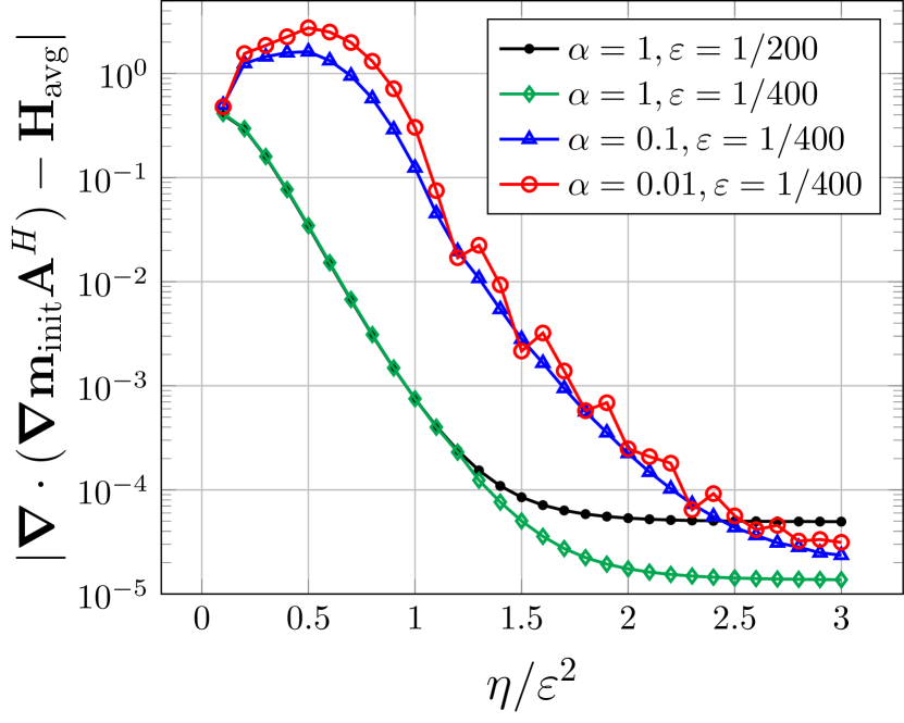
Refer to caption
(a) Averaging error Eavgsubscript𝐸avgE_{\mathrm{avg}} when varying Ξ·πœ‚\eta.
Refer to caption
(b) Time required until Eavgsubscript𝐸avgE_{\mathrm{avg}} falls below given thresholds when varying α𝛼\alpha.
Figure 13: (EX2): Influence of the time averaging length Ξ·πœ‚\eta on the overall error in one micro problem. Here ΞΌ=3.9β€‹Ξ΅πœ‡3.9πœ€\mu=3.9\varepsilon and ΞΌβ€²superscriptπœ‡β€²\mu^{\prime} is chosen sufficiently big to not significantly change the results. Kernel parameters pt=3subscript𝑝𝑑3p_{t}=3 and qt=7subscriptπ‘žπ‘‘7q_{t}=7.

In FigureΒ 13(b), we further investigate the influence of the damping parameter on the time Ξ·πœ‚\eta it takes for the averaging error Eavgsubscript𝐸avgE_{\mathrm{avg}} to fall below certain given thresholds. One can clearly observe that high damping reduces the required time to reach all three considered error levels. This indicates that the introduction of artificial damping in the micro problem can help to significantly reduce computational cost, since a shorter final time also implies a smaller computational domain as explained in the previous section. However, since α≫1much-greater-than𝛼1\alpha\gg 1 results in a seriously increased number of time steps necessary to get a stable solution, as discussed in SectionΒ 3.2, we conclude that choosing α𝛼\alpha around one is most favorable.

Example (EX3)

To support the considerations regarding the choice of micro parameters, we furthermore study the Landau-Lifshitz problem 2.2 with the setup (EX3). In (EX3) the material coefficient has a higher average and higher maximum value than in (EX2). This results in a higher β€œspeed” of the dynamics. In FigureΒ 14, the influence of ΞΌπœ‡\mu, ΞΌβ€²superscriptπœ‡β€²\mu^{\prime}, Ξ·πœ‚\eta and α𝛼\alpha, respectively, on the averaging error Eavgsubscript𝐸avgE_{\mathrm{avg}} are shown for this example.

Refer to caption
(a) Influence of averaging domain parameter ΞΌπœ‡\mu, compare to FigureΒ 11.
Refer to caption
(b) Influence of computational domain extension ΞΌβ€²βˆ’ΞΌsuperscriptπœ‡β€²πœ‡\mu^{\prime}-\mu, see FigureΒ 12.
Refer to caption
(c) Influence of averaging time Ξ·πœ‚\eta, compare to FigureΒ 13(a).
Refer to caption
(d) Influence of damping α𝛼\alpha, compare to FigureΒ 13(b).
Figure 14: (EX3): Influence of micro domain parameters on error Eavgsubscript𝐸avgE_{\mathrm{avg}}. Parameters not explicitly given are chosen to not influence Eavgsubscript𝐸avgE_{\mathrm{avg}} significantly. Moreover, Ξ΅=1/400πœ€1400\varepsilon=1/400, and Ξ±=1𝛼1\alpha=1 in (a) - (c).

Qualitatively, the results for (EX3) are the same as (EX2), but some details differ. A notable difference between the examples (EX2) and (EX3) is that the time Ξ·πœ‚\eta required for saturation of the errors is considerably shorter in (EX3), as can be observed when comparing FigureΒ 14(c) to FigureΒ 13(a). An explanation for this is that due to the faster dynamics in (EX3), comparable effects are achieved at shorter times. The ratio between the times Ξ·πœ‚\eta it takes in (EX2) and (EX3), respectively, to reach the level where the error no longer changes matches approximately with the ratio of the maxima of the material coefficients.

Moreover, a slightly larger ΞΌπœ‡\mu is required to reach the level where the errors saturate in (EX3). The (EX3) saturation errors for a specific value of Ξ·πœ‚\eta are lower, though, due to the fact that the error decreases faster with Ξ·πœ‚\eta as discussed previously.

When it comes to the full size of the domain required for the boundary error to not influence the overall error in a significant way, one can observe somewhat larger required value of ΞΌβ€²superscriptπœ‡β€²\mu^{\prime} in (EX3) when comparing FigureΒ 14(b) to FigureΒ 12. This is partly due to the fact that the overall error for a given Ξ·πœ‚\eta is lower in (EX3). Moreover, due to the faster dynamics, the errors at time Ξ·πœ‚\eta have propagated further into the domain. As a result, the computational domain has to be chosen approximately the same size in (EX2) and (EX3) to obtain a certain error level, even though the required Ξ·πœ‚\eta is smaller in (EX3).

4.4 Computational Cost

The computational cost per micro problem is a major factor for an efficient HMM implementation. Given a spatial discretization with a certain number of grid points, K𝐾K, per wave length Ξ΅πœ€\varepsilon, that is a micro grid spacing δ​x=Ξ΅/K𝛿π‘₯πœ€πΎ\delta x=\varepsilon/K, we have in total Nd=(2​K​μ′/Ξ΅)dsuperscript𝑁𝑑superscript2𝐾superscriptπœ‡β€²πœ€π‘‘N^{d}=\left(2K\mu^{\prime}/\varepsilon\right)^{d} micro grid points. The time step size for the micro time integration has to be chosen as δ​t≀Cstab,α​δ​x2𝛿𝑑subscript𝐢stab𝛼𝛿superscriptπ‘₯2\delta t\leq C_{\mathrm{stab,\alpha}}\delta x^{2}, hence the number of time steps becomes Mβ‰₯Cstab,Ξ±βˆ’1​K2​η/Ξ΅2𝑀superscriptsubscript𝐢stab𝛼1superscript𝐾2πœ‚superscriptπœ€2M\geq C_{\mathrm{stab,\alpha}}^{-1}K^{2}\eta/\varepsilon^{2}. It then holds for the computational cost per micro problem that

micro​cost∼M​Nd∼1Cs​t​a​b,Ξ±micro​ηΡ2​(ΞΌβ€²Ξ΅)d​K2+d.similar-tomicrocost𝑀superscript𝑁𝑑similar-to1subscriptπΆπ‘ π‘‘π‘Žπ‘subscript𝛼microπœ‚superscriptπœ€2superscriptsuperscriptπœ‡β€²πœ€π‘‘superscript𝐾2𝑑\displaystyle\mathrm{micro~{}cost}\sim MN^{d}\sim\frac{1}{C_{stab,\alpha_{\mathrm{micro}}}}\frac{\eta}{\varepsilon^{2}}\left(\frac{\mu^{\prime}}{\varepsilon}\right)^{d}K^{2+d}. (4.39)

It is important to note that due to the choice of parameters ΞΌβ€²βˆΌΞ΅similar-tosuperscriptπœ‡β€²πœ€\mu^{\prime}\sim\varepsilon and η∼Ρ2similar-toπœ‚superscriptπœ€2\eta\sim\varepsilon^{2}, the computational cost per micro problem is independent of Ξ΅πœ€\varepsilon. This makes it possible to use HMM also for problems where the computational cost of other approaches, resolving the fast oscillations, becomes tremendously high.

In general, choosing higher values for Ξ·,ΞΌβ€²πœ‚superscriptπœ‡β€²\eta,\mu^{\prime} or K𝐾K results in higher computational cost per micro problem. We therefore aim to choose these values as low as possible without negatively affecting the overall error. The overall cost is determined by the cost per micro problem and the choice of the macro discretization size Δ​XΔ𝑋\Delta X,

cost∼1Cstab,Ξ±macro​(Δ​X)βˆ’(2+d)​micro​cost.similar-tocost1subscript𝐢stabsubscript𝛼macrosuperscriptΔ𝑋2𝑑microcost\mathrm{cost}\sim\frac{1}{C_{\mathrm{stab,\alpha_{\mathrm{macro}}}}}(\Delta X)^{-(2+d)}\mathrm{micro~{}cost}.

This shows the importance of choosing Δ​XΔ𝑋\Delta X relatively large, wherefore it is advantageous that the overall method proposed based on MPEA is fourth order accurate, as discussed in SectionΒ 3.3. Since all the HMM micro problems are independent of each other, it is moreover very simple to parallelize their computations. This can be an effective way to reduce the overall run time of the method.

4.5 Choice of overall setup

According to sectionΒ 4, the overall approximation error in 𝐇avgsubscript𝐇avg\mathbf{H}_{\mathrm{avg}} is

Eapprox=Eavg+Edisc,subscript𝐸approxsubscript𝐸avgsubscript𝐸discE_{\mathrm{approx}}=E_{\mathrm{avg}}+E_{\mathrm{disc}},

where Ediscsubscript𝐸discE_{\mathrm{disc}} is determined by the macro discretization size Δ​XΔ𝑋\Delta X as given in 4.36. For a given Δ​XΔ𝑋\Delta X, we therefore aim to choose the parameters ΞΌ,ΞΌβ€²πœ‡superscriptπœ‡β€²\mu,\mu^{\prime} and Ξ·πœ‚\eta so that Eavgsubscript𝐸avgE_{\mathrm{avg}} matches Ediscsubscript𝐸discE_{\mathrm{disc}}. Further reducing Eavgsubscript𝐸avgE_{\mathrm{avg}} only increases the computational cost per micro problem without significantly improving the overall error.

The specific values of the discretization error depend on the given macro solution and macro location. We here take as an example the macro initial data and the micro problem solved to obtain 𝐇avgsubscript𝐇avg\mathbf{H}_{\mathrm{avg}} at macro location (0,0)00(0,0). We consider Δ​X=1/(12β‹…2i)Δ𝑋1β‹…12superscript2𝑖\Delta X=1/(12\cdot 2^{i}), i=0,1,2𝑖012i=0,1,2 and suggest in TableΒ 1 choices for Ξ·πœ‚\eta and ΞΌβ€²superscriptπœ‡β€²\mu^{\prime} in the example setups (EX2) and (EX3) such that Eavgsubscript𝐸avgE_{\mathrm{avg}} is slightly below the corresponding values for Ediscsubscript𝐸discE_{\mathrm{disc}} when using fourth order interpolation. The averaging parameter ΞΌπœ‡\mu is fixed to a value such that EΞΌsubscriptπΈπœ‡E_{\mu} does not significantly increase Eavgsubscript𝐸avgE_{\mathrm{avg}} but not much higher. This helps to reduce the number of parameters to vary. Moreover, choosing lower ΞΌπœ‡\mu results in a rather steep increase of Eavgsubscript𝐸avgE_{\mathrm{avg}} in comparison to how much the computational cost is reduced. We furthermore choose Ξ±=1𝛼1\alpha=1 here to make it simple to compare the suggestions to the values shown in FiguresΒ 13(a), 12 andΒ 11 as well as FigureΒ 14. The optimal choice for α𝛼\alpha would be slightly higher.

(EX2) (EX3)
Δ​XΔ𝑋\Delta X Ediscsubscript𝐸discE_{\mathrm{disc}} Ξ·/Ξ΅2πœ‚superscriptπœ€2\eta/\varepsilon^{2} amax​η/Ξ΅2subscriptπ‘Žmaxπœ‚superscriptπœ€2a_{\mathrm{max}}\eta/\varepsilon^{2} (ΞΌβ€²βˆ’ΞΌ)/Ξ΅superscriptπœ‡β€²πœ‡πœ€(\mu^{\prime}-\mu)/\varepsilon Ξ·/Ξ΅2πœ‚superscriptπœ€2\eta/\varepsilon^{2} amax​η/Ξ΅2subscriptπ‘Žmaxπœ‚superscriptπœ€2a_{\mathrm{max}}\eta/\varepsilon^{2} (ΞΌβ€²βˆ’ΞΌ)/Ξ΅superscriptπœ‡β€²πœ‡πœ€(\mu^{\prime}-\mu)/\varepsilon
1/12 2.3β‹…10βˆ’2β‹…2.3superscript1022.3\cdot 10^{-2} 0.7 1.09 4 0.4 1.02 3
1/24 1.6β‹…10βˆ’3β‹…1.6superscript1031.6\cdot 10^{-3} 1 1.56 6 0.6 1.53 5
1/48 1β‹…10βˆ’4β‹…1superscript1041\cdot 10^{-4} 1.4 2.18 8 0.8 2.05 7
Table 1: Example micro problem setups with Ξ±=1𝛼1\alpha=1, where ΞΌ=3.9β€‹Ξ΅πœ‡3.9πœ€\mu=3.9\varepsilon for (EX2) and ΞΌ=4.2β€‹Ξ΅πœ‡4.2πœ€\mu=4.2\varepsilon for (EX3) .

Based on the values in TableΒ 1, one can conclude that the required sizes of the computational domains are very similar between the considered examples. When scaled by the maximum of the respective material coefficients, also the suggested final times are comparable.

To further test the influence of the micro domain setup and corresponding Eavgsubscript𝐸avgE_{\mathrm{avg}} on the overall error, we consider (EX2) on a unit square domain with periodic boundary condition, Ξ±=0.01𝛼0.01\alpha=0.01 in the original problem and a final time T=0.1𝑇0.1T=0.1. We use artificial damping and set Ξ±=1.2𝛼1.2\alpha=1.2 in the micro problem. As in the previous examples, we choose averaging kernel parameters px=pt=3subscript𝑝π‘₯subscript𝑝𝑑3p_{x}=p_{t}=3 and qx=qt=7subscriptπ‘žπ‘₯subscriptπ‘žπ‘‘7q_{x}=q_{t}=7 and let Ξ΅=1/400πœ€1400\varepsilon=1/400. We again fix ΞΌ=3.9β€‹Ξ΅πœ‡3.9πœ€\mu=3.9\varepsilon, and run HMM with MPEA for the macro time stepping to approximate the homogenized reference solution 𝐌0subscript𝐌0\mathbf{M}_{0} at time T𝑇T for varying Δ​XΔ𝑋\Delta X.

Refer to caption
Ξ·/Ξ΅2πœ‚superscriptπœ€2\eta/\varepsilon^{2} ΞΌβ€²superscriptπœ‡β€²\mu^{\prime} Eavgsubscript𝐸avgE_{\mathrm{avg}}
s1 0.15 4 β‰ˆ3β‹…10βˆ’1absentβ‹…3superscript101\approx 3\cdot 10^{-1}
s2 0.45 5.5 β‰ˆ3β‹…10βˆ’2absentβ‹…3superscript102\approx 3\cdot 10^{-2}
s3 0.7 7.5 β‰ˆ3β‹…10βˆ’3absentβ‹…3superscript103\approx 3\cdot 10^{-3}
s4 1 10 β‰ˆ3β‹…10βˆ’4absentβ‹…3superscript104\approx 3\cdot 10^{-4}
Micro problem setups for (EX2) (with Ξ±=1.2𝛼1.2\alpha=1.2 and ΞΌ=3.9πœ‡3.9\mu=3.9) and resulting Eavgsubscript𝐸avgE_{\mathrm{avg}} in micro problem at macro location x0=(0,0)subscriptπ‘₯000x_{0}=(0,0).
Figure 15: L2superscript𝐿2L^{2}-norm of difference between HMM solution 𝐌𝐌\mathbf{M} and homogenized reference solution 𝐌0subscript𝐌0\mathbf{M}_{0} at time T=0.1𝑇0.1T=0.1 for (EX2).

Four different combinations of Ξ·πœ‚\eta and ΞΌβ€²superscriptπœ‡β€²\mu^{\prime} are used for the micro problem, referred to as (s1)-(s4). The resulting L2superscript𝐿2L^{2}-norms of the errors 𝐌0βˆ’πŒsubscript𝐌0𝐌\mathbf{M}_{0}-\mathbf{M} are shown in FigureΒ 15, together with the error one obtains when using the average aavgsubscriptπ‘Žavga_{\mathrm{avg}} of the material coefficient aΞ΅superscriptπ‘Žπœ€a^{\varepsilon} to approximate 𝐀Hsuperscript𝐀𝐻\mathbf{A}^{H} when solving 2.3. Using aavgsubscriptπ‘Žavga_{\mathrm{avg}} can be seen as a naive approach to dealing with the fast oscillations in the material coefficient. It does in general not result in good approximations. The corresponding error is included here to give a baseline for the relevance of the HMM solutions.

We find that with the micro problem setup (s1), corresponding to a rather high averaging error, HMM results in a solution that is only slightly better than the one that is obtained using the average of the material coefficient. However, when applying setups with lower averaging errors, lower overall errors are achieved. In particular, with (s4), the setup with the lowest considered averaging error, the overall error in FigureΒ 15 is determined by the error Ediscsubscript𝐸discE_{\mathrm{disc}}, proportional to (Δ​X)4superscriptΔ𝑋4(\Delta X)^{4} since fourth order interpolation is used to obtain the initial data for the micro problems. For the other two setups, (s2) and (s3), the overall errors saturate at levels somewhat lower than the respective values of Eavgsubscript𝐸avgE_{\mathrm{avg}}, corresponding to eHMMsubscript𝑒HMMe_{\mathrm{HMM}} in 3.27. Note that this saturation occurs for relatively high values of Δ​XΔ𝑋\Delta X.

5 Further numerical examples

To conclude this article, we consider several numerical examples with material coefficients that are not fully periodic. Those cases are not covered by the theorems in SectionΒ 2, however, the HMM approach still results in good approximations. In the 2D examples, we again include the solution obtained when using a (local) average of the material coefficient as an approximation to the effective coefficient to stress the relevance of the HMM solutions. As for the periodic examples, we use artificial damping in the micro problem.

Locally periodic 1D example

We first consider a one-dimensional example with material coefficient

aΡ​(x)=1.1+14​sin⁑(2​π​x+1.1)+12​sin⁑(2​π​x/Ξ΅).superscriptπ‘Žπœ€π‘₯1.1142πœ‹π‘₯1.1122πœ‹π‘₯πœ€a^{\varepsilon}(x)=1.1+\tfrac{1}{4}\sin(2\pi x+1.1)+\tfrac{1}{2}\sin(2\pi x/\varepsilon). (5.40)

This coefficient is locally periodic. We consider 2.2 with this coefficient and Ξ΅=1/400πœ€1400\varepsilon=1/400, Ξ±=0.01𝛼0.01\alpha=0.01 on the unit interval with periodic boundary conditions. A comparison between the solution 𝐌ΡsuperscriptπŒπœ€\mathbf{M}^{\varepsilon} at time T=0.1𝑇0.1T=0.1, obtained using a direct numerical simulation resolving the Ξ΅πœ€\varepsilon-scale, and corresponding HMM approximation on a coarse grid with Δ​X=1/24Δ𝑋124\Delta X=1/24 is shown in FigureΒ 16. Here the HMM parameters are chosen to be ΞΌ=3.9β€‹Ξ΅πœ‡3.9πœ€\mu=3.9\varepsilon, ΞΌβ€²=8​Ρsuperscriptπœ‡β€²8πœ€\mu^{\prime}=8\varepsilon and Ξ·=0.9​Ρ2πœ‚0.9superscriptπœ€2\eta=0.9\varepsilon^{2}. Artificial damping with Ξ±=1.2𝛼1.2\alpha=1.2 is used for the micro problem. The averaging kernel parameters are again px=pt=3subscript𝑝π‘₯subscript𝑝𝑑3p_{x}=p_{t}=3 and qx=qt=7subscriptπ‘žπ‘₯subscriptπ‘žπ‘‘7q_{x}=q_{t}=7.

Refer to caption
Figure 16: HMM solution to 2.2 with aΞ΅superscriptπ‘Žπœ€a^{\varepsilon} as in 5.40 with Ξ΅=1/400πœ€1400\varepsilon=1/400 and corresponding 𝐌ΡsuperscriptπŒπœ€\mathbf{M}^{\varepsilon} obtained using direct simulation resolving Ξ΅πœ€\varepsilon, at T=0.1𝑇0.1T=0.1.

For the direct simulation, we use Δ​x=1/6000Ξ”π‘₯16000\Delta x=1/6000, which corresponds to 15 grid points per Ξ΅πœ€\varepsilon, and MPEA for time integration.

One can clearly observe that the HMM solution is very close to the solution obtained with a direct simulation resolving Ξ΅πœ€\varepsilon. Moreover, note that in this example the computation time for HMM is about 15 seconds111on a computer with Intel i7-4770 CPU at 3.4 GHz, while the direct simulation takes almost two hours.

Quasi-periodic 2D example

Next, 2.2 is solved in two space dimensions and with material coefficient

aΡ​(x)=(1+0.25​sin⁑(2​π​x1/Ξ΅))​(1+0.25​sin⁑(2​π​x2/Ξ΅)+0.25​sin⁑(2​π​r​x2/Ξ΅)),superscriptπ‘Žπœ€π‘₯10.252πœ‹subscriptπ‘₯1πœ€10.252πœ‹subscriptπ‘₯2πœ€0.252πœ‹π‘Ÿsubscriptπ‘₯2πœ€\displaystyle a^{\varepsilon}(x)=(1+0.25\sin(2\pi x_{1}/\varepsilon))(1+0.25\sin(2\pi x_{2}/\varepsilon)+0.25\sin(2\pi rx_{2}/\varepsilon)), (5.41)

where r=1.41π‘Ÿ1.41r=1.41 as an approximation to 22\sqrt{2}. This coefficient is periodic in x1subscriptπ‘₯1x_{1}-direction but not in x2subscriptπ‘₯2x_{2}-direction. If we choose Ξ΅=0.01πœ€0.01\varepsilon=0.01, though, it is periodic also in x2subscriptπ‘₯2x_{2} direction over the whole domain [0,1]2superscript012[0,1]^{2} but not on the micro domains. The initial data is set as in (EX2).

To make direct numerical simulation feasible, we consider the case Ξ΅=0.01πœ€0.01\varepsilon=0.01 and set Δ​x=1/1500Ξ”π‘₯11500\Delta x=1/1500 in the direct simulation. For HMM, the micro problem parameters are chosen to be ΞΌ=6.5β€‹Ξ΅πœ‡6.5πœ€\mu=6.5\varepsilon, Ξ·=0.7​Ρ2πœ‚0.7superscriptπœ€2\eta=0.7\varepsilon^{2} and ΞΌβ€²=9​Ρsuperscriptπœ‡β€²9πœ€\mu^{\prime}=9\varepsilon. We use again averaging kernels with px=pt=3subscript𝑝π‘₯subscript𝑝𝑑3p_{x}=p_{t}=3 and qx=qt=7subscriptπ‘žπ‘₯subscriptπ‘žπ‘‘7q_{x}=q_{t}=7 as well as artificial damping with Ξ±=1.2𝛼1.2\alpha=1.2 in the micro problem. On the macro scale, Δ​X=1/16Δ𝑋116\Delta X=1/16. The final time is set to T=0.2𝑇0.2T=0.2.

In FigureΒ 17(a), the xπ‘₯x-components of 𝐌ΡsuperscriptπŒπœ€\mathbf{M}^{\varepsilon}, obtained using a direct simulation resolving Ξ΅πœ€\varepsilon and a HMM solution to 2.2 with material coefficient 5.41 are shown. Moreover, the solution obtained when simply using the average of aΡ​(x)superscriptπ‘Žπœ€π‘₯a^{\varepsilon}(x) as an approximation is included. One can observe that the HMM solution captures the characteristics of the overall solution well, while the approach with an averaged coefficient does not. To further stress this, cross sections of the respective solutions at x1=0.5subscriptπ‘₯10.5x_{1}=0.5 and x2=0.5subscriptπ‘₯20.5x_{2}=0.5 are shown in FigureΒ 17(b).

Refer to caption
(a) Contours
Refer to caption
Refer to caption
(b) Cross sections
Figure 17: Quasi-periodic example, with Ξ΅=0.01πœ€0.01\varepsilon=0.01, T=0.2𝑇0.2T=0.2 and Ξ±=0.01𝛼0.01\alpha=0.01.

Despite the choice of a rather high Ξ΅πœ€\varepsilon-value, Ξ΅=0.01πœ€0.01\varepsilon=0.01, the direct simulation of this problem took about 5 days. In comparison, the computational time of HMM was about 4 hours, which is independent of Ξ΅πœ€\varepsilon.

Locally periodic 2D example

Finally, we consider a locally periodic 2D example with material coefficient

aΡ​(x)=0.25​exp⁑(βˆ’cos⁑(2​π​(x1+x2)/Ξ΅)+sin⁑(2​π​x1/Ξ΅)​cos⁑(2​π​x2)).superscriptπ‘Žπœ€π‘₯0.252πœ‹subscriptπ‘₯1subscriptπ‘₯2πœ€2πœ‹subscriptπ‘₯1πœ€2πœ‹subscriptπ‘₯2\displaystyle a^{\varepsilon}(x)=0.25\exp\left(-\cos(2\pi(x_{1}+x_{2})/\varepsilon)+\sin(2\pi x_{1}/\varepsilon)\cos(2\pi x_{2})\right). (5.42)

In this example, we set Ξ±=0.1𝛼0.1\alpha=0.1 and choose a final time T=0.05𝑇0.05T=0.05.

The HMM parameters are set to ΞΌ=5β€‹Ξ΅πœ‡5πœ€\mu=5\varepsilon, ΞΌβ€²=7​Ρsuperscriptπœ‡β€²7πœ€\mu^{\prime}=7\varepsilon and Ξ·=1.1​Ρ2πœ‚1.1superscriptπœ€2\eta=1.1\varepsilon^{2}. Again Ξ±=1.2𝛼1.2\alpha=1.2 in the micro problem. Initial data and averaging parameters are set as in the previous example. Direct simulation solution 𝐌ΡsuperscriptπŒπœ€\mathbf{M}^{\varepsilon}, HMM approximation and a solution based on local averages of aΞ΅superscriptπ‘Žπœ€a^{\varepsilon} are shown in FigureΒ 18. Also for this problem HMM captures the characteristics of the solution well, in contrast to the averaging based solution.
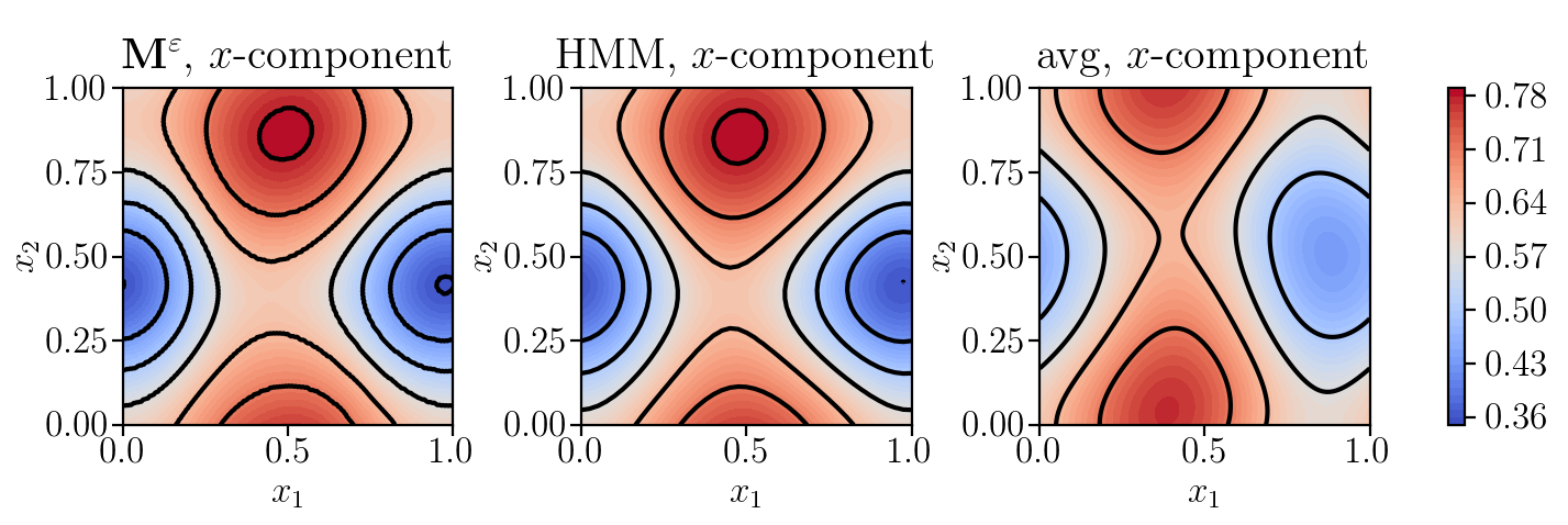
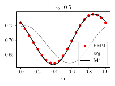
Refer to caption
(a) Contours
Refer to caption
Refer to caption
(b) Cross sections
Figure 18: Locally periodic example, with Ξ΅=0.01πœ€0.01\varepsilon=0.01, T=0.05𝑇0.05T=0.05 and Ξ±=0.1𝛼0.1\alpha=0.1.

References

  • [1] Abdulle, A., E, W., Engquist, B., and Vanden-Eijnden, E. The Heterogeneous Multiscale Method. Acta Numerica 21 (2012), 1–87.
  • [2] Alouges, F., DeΒ Bouard, A., Merlet, B., and Nicolas, L. Stochastic homogenization of the Landau-Lifshitz-Gilbert equation. Stochastics and Partial Differential Equations: Analysis and Computations (2021), 1–30.
  • [3] Arjmand, D., Engblom, S., and Kreiss, G. Temporal upscaling in micromagnetism via heterogeneous multiscale methods. J. Comput. Appl. Math. 345 (2019), 99–113.
  • [4] Arjmand, D., Kreiss, G., and Poluektov, M. Atomistic-continuum multiscale modeling of magnetization dynamics at non-zero temperature. Adv. Comput. Math 44 (2018), 1119–1151.
  • [5] Arjmand, D., and Runborg, O. Analysis of heterogeneous multiscale methods for long time wave propagation problems. Multiscale Modeling & Simulation 12, 3 (2014), 1135–1166.
  • [6] Arjmand, D., and Runborg, O. A time dependent approach for removing the cell boundary error in elliptic homogenization problems. Journal of Computational Physics 314 (2016), 206–227.
  • [7] Baňas, L. Numerical methods for the Landau-Lifshitz-Gilbert equation. In International Conference on Numerical Analysis and Its Applications (2004), Springer, pp.Β 158–165.
  • [8] Choquet, C., Moumni, M., and Tilioua, M. Homogenization of the Landau-Lifshitz-Gilbert equation in a contrasted composite medium. Discrete & Continuous Dynamical Systems-S 11, 1 (2018), 35.
  • [9] CimrΓ‘k, I. A survey on the numerics and computations for the Landau-Lifshitz equation of micromagnetism. Archives of Computational Methods in Engineering 15, 3 (2007), 1–37.
  • [10] d’Aquino, M., Serpico, C., and Miano, G. Geometrical integration of Landau–Lifshitz–Gilbert equation based on the mid-point rule. Journal of Computational Physics 209, 2 (2005), 730–753.
  • [11] d’Aquino, M., Serpico, C., Miano, G., Mayergoyz, I., and Bertotti, G. Numerical integration of Landau–Lifshitz–Gilbert equation based on the midpoint rule. Journal of applied physics 97, 10 (2005), 10E319.
  • [12] E, W., Engquist, B., etΒ al. The Heterognous Multiscale Methods. Communications in Mathematical Sciences 1, 1 (2003), 87–132.
  • [13] E, W., Engquist, B., Li, X., Ren, W., and Vanden-Eijnden, E. Heterogeneous Multiscale Methods: a review. Communications in computational physics 2, 3 (2007), 367–450.
  • [14] E, W., and Wang, X.-P. Numerical methods for the Landau-Lifshitz equation. SIAM journal on numerical analysis (2001), 1647–1665.
  • [15] Engquist, B., and Tsai, Y.-H. Heterogeneous multiscale methods for stiff ordinary differential equations. Mathematics of computation 74, 252 (2005), 1707–1742.
  • [16] GarcΓ­a-Cervera, C.Β J. Numerical micromagnetics: A review.
  • [17] GarcΓ­a-Cervera, C.Β J., etΒ al. Improved Gauss-Seidel projection method for micromagnetics simulations. IEEE transactions on magnetics 39, 3 (2003), 1766–1770.
  • [18] Hamdache, K. Homogenization of layered ferromagnetic media. Ecole Polytechnique, Centre de MathΓ©matiques AppliquΓ©es, R. I. No 495, http://www.cmap.polytechnique.fr/ preprint/repository/495.ps (gzip archive), 2002.
  • [19] Krishnaprasad, P.Β S., and Tan, X. Cayley transforms in micromagnetics. Physica B: Condensed Matter 306, 1-4 (2001), 195–199.
  • [20] Leitenmaier, L. Heterogeneous Multiscale Methods for the Landau-Lifshitz equation, 2021.
  • [21] Leitenmaier, L., and Runborg, O. On homogenization of the Landau-Lifshitz equation with rapidly oscillating material coefficient. arXiv preprint, arXiv:2012.12567 (2020).
  • [22] Leitenmaier, L., and Runborg, O. Upscaling errors in heterogeneous multiscale models for the Landau-Lifshitz equation. arXiv preprint, arXiv:2104.03206 (2021).
  • [23] Lewis, D., and Nigam, N. Geometric integration on spheres and some interesting applications. Journal of Computational and Applied Mathematics 151, 1 (2003), 141–170.
  • [24] Li, P., Xie, C., Du, R., Chen, J., and Wang, X.-P. Two improved Gauss-Seidel projection methods for Landau-Lifshitz-Gilbert equation. Journal of Computational Physics 401 (2020), 109046.
  • [25] Mayergoyz, I.Β D., Bertotti, G., and Serpico, C. Nonlinear magnetization dynamics in nanosystems. Elsevier, 2009.
  • [26] Mentink, J., Tretyakov, M., Fasolino, A., Katsnelson, M., and Rasing, T. Stable and fast semi-implicit integration of the stochastic Landau–Lifshitz equation. Journal of Physics: Condensed Matter 22, 17 (2010), 176001.
  • [27] PeirΓ³, J., and Sherwin, S. Finite Difference, Finite Element and Finite Volume Methods for Partial Differential Equations. Handbook of Materials Modeling: Methods. Springer Netherlands, Dordrecht, 2005, pp.Β 2415–2446.
  • [28] Santugini-Repiquet, K. Homogenization of ferromagnetic multilayers in the presence of surface energies. ESAIM: Control, Optimisation and Calculus of Variations 13, 2 (2007), 305–330.
  • [29] Serpico, C., Mayergoyz, I., and Bertotti, G. Numerical technique for integration of the Landau–Lifshitz equation. Journal of Applied Physics 89, 11 (2001), 6991–6993.
  • [30] Wang, X.-P., GarcΔ±a-Cervera, C.Β J., and E, W. A Gauss–Seidel projection method for micromagnetics simulations. Journal of Computational Physics 171, 1 (2001), 357–372.
  • [31] Wei, D. Micromagnetics and recording materials. Springer Science & Business Media, 2012.