Analyze and Design Network Architectures by Recursion Formulas

Abstract

The effectiveness of shortcut/skip-connection has been widely verified, which inspires massive explorations on neural architecture design. This work attempts to find an effective way to design new network architectures.

it is discovered that the main difference between network architectures can be reflected in their recursion formulas. Based on this, a methodology is proposed to design novel network architectures from the perspective of mathematical formulas.

Afterwards, a case study is provided to generate an improved architecture based on ResNet.

Furthermore, the new architecture is compared with ResNet and then tested on ResNet-based networks. Massive experiments are conducted on CIFAR and ImageNet, which witnesses the significant performance improvements provided by the architecture.

1 Introduction

Years of practice has proved that convolutional neural network(CNN) is a significantly important deep learning method in the field of image recognition. Many new architectures of CNN have been proposed and have achieved good performance[17, 18, 19, 20, 21, 22, 23]. With the proposal of highway network[1] and residual network[2], skip-connection and shortcut are widely used in deep CNNs[4, 5, 6, 7, 8], which results in CNNs with amazing depth. Residual networks have then achieved subversive performance in a variety of visual tasks[2, 3]. As a consequence, shortcut has now become an essential component of most deep networks.

The successful application of skip-connection and shortcut has led to a series of research explorations on the CNN architecture, e.g., DenseNet[5], Feedback Network[9], EfficientNet[8], etc. Models designed to improve block performance have also appeared one after another, e.g., SEResNet[4], ResNeXt[6], Res2Net[7], etc. With the emergence of these amazing research work and the reviews[10, 11, 12] of previous work, we begin to think about the question that

Can we find an effective method to design architectures of networks?

Can the new network architecture is designed according to our goal?

In this paper, we first analyze and compare the CNNs with and without shortcut — take the partial derivative of the output of the last layer/block with respect to the output of a previous layer/block to make the propagation paths in the networks be presented in a mathematical formula. By comparison, it is discovered that it is the difference in network recursion formulas that causes the huge difference between the the CNNs without and with shortcut. In addition, a new interpretation of the residual network is obtained by partial derivative analysis.

By the comparative analysis of the two types of networks, the significance of recursion formulas to network architecture highlights. So, by the reasonable design of network recursion formulas, networks with different architectures can be further designed as Figure 1.

Figure 1: The flow chart of the proposed method

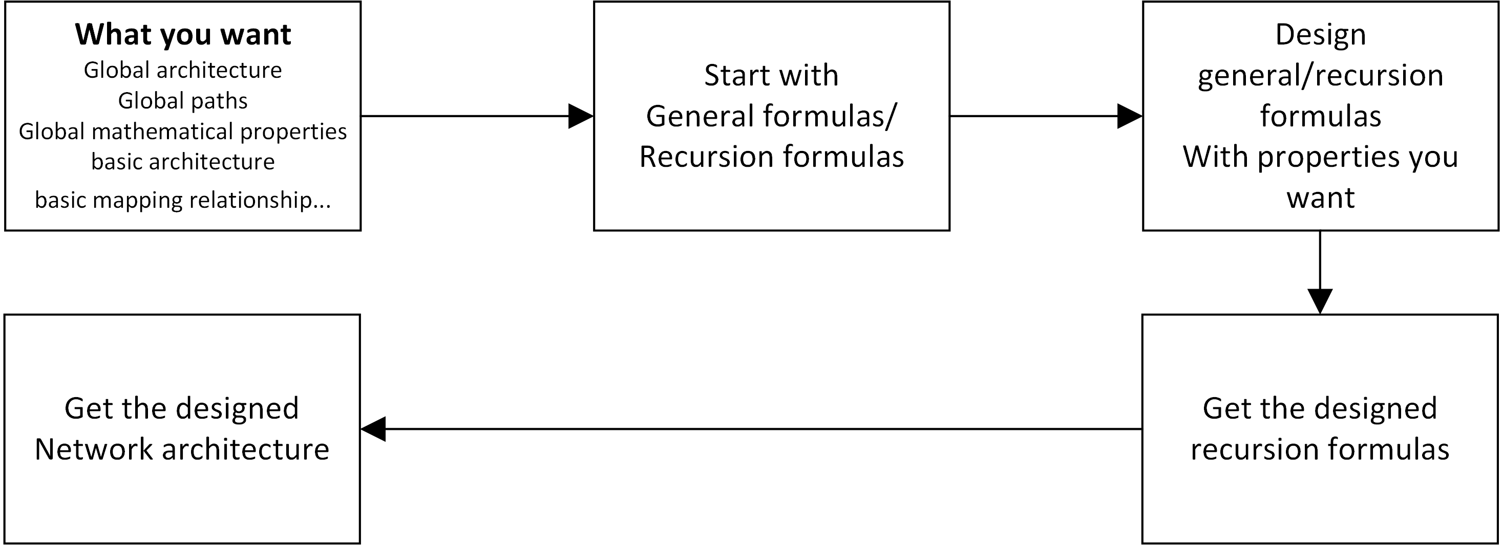
By the guide of this idea, we take ResNet as an example, make some modifications to the general formula of ResNet and a new recursion formula is obtained, based on which we design a novel architecture. We evaluate the new architecture on CIFAR[13] and ImageNet[14] data sets, and it has better performance compared with ResNet. Further, we test the generality and compatibility of the new architecture with other popular networks . Experiments show that networks based on the newly designed architecture have improvement in performance compared to themselves before.

2 Related Work

Highway network

Highway networks[1] present shortcut connections with gating functions[16]. The output of each layer of a highway network is defined as[10]

$$y_{i+1}\equiv f_{i+1}\left(y_{i}\right)\cdot t_{i+1}\left(y_{i}\right)+y_{i}\cdot\left(1-t_{i+1}\left(y_{i}\right)\right),$$ (1)

where $y_{i+1}$ and $y_{i}$ denote the output and input of $i$-th layer, $t_{i+1}$ denotes the gate function of $(i+1)$-th layer, $f_{i+1}\left(x\right)$ denotes some sequence of convolutions. Eq.(1) is actually the recursion formula of highway networks. And highway network is one of the networks to embody the network architecture in the network recursion formula.

Residual network

Identity mapping allows neural networks to reach a depth that was unimaginable before. In the analysis of the residual network[2, 3], the recursion formula plays a vital role. Residual unit performs the following computation:

$$\begin{array}[]{c}\mathbf{y}_{l}=h\left(\mathrm{x}_{l}\right)+F\left(\mathrm{x}_{l},\omega_{l}\right)\\ \mathrm{x}_{l+1}=fp\left(\mathrm{y}_{l}\right)\end{array},$$ (2)

where, $\mathrm{x}_{l}$ and $\mathrm{x}_{l+1}$ are the input and output the $l$-th residual unit, $\omega_{l}$ is a set of weights (and biases) associated with the $l$-th residual unit. The function $fp$ is the operation after element-wise addition. The function $h$ is set as an identity mapping:$h\left(\mathrm{x}_{l}\right)=\mathrm{x}_{l}$.

Furthermore, partial derivation is used to analyze the relationship between the outputs of units. Paper[3] analyzes the meaning of each item in the partial derivative formula in the network, and it is proved in the meanwhile that shortcut ensures that information can be directly propagated back to any shallower unit. Our work is parallel to this and gives a further view on this basis that the recursion formula is the embodiment of architecture and partial derivative formulas can be used to study the propagation paths in the network.

Study on the architecture of ResNet

Paper[10] analyzes the architecture of residual networks and comes to a conclusion that residual networks behave like ensembles of relatively shallow networks. This work shows the propagation paths that residual network contains by forward derivation of the recursion formula. We come to a similar conclusion by the partial derivative of the output of the last block with respect to the output of a previous block.

3 Analysis

3.1 Analysis of Traditional CNNs

For the traditional convolutional neural networks[15], the recursion formula is:

$$X_{i}=g_{i}\left[F\left(X_{i-1},\theta_{i}\right)\right],0<i<L+1$$ (3)

where $L$ is the total number of layers, $X_{i}$ denotes the output of $i$-th layer, $g_{i}$ denotes the activation function of $i$-th layer , $F$ denotes the mapping of the layer from input to output and $\theta_{i}$ denotes the parameter of $i$-th layer.

In order to make the propagation paths in the network easy to understand, we take the partial derivative of the output of the last block with respect to the output of a previous block[3]:

$$\frac{\partial X_{L}}{\partial X_{L-1}}=g_{L}^{\prime}\cdot W_{L}$$ (4)

$$\frac{\partial X_{L}}{\partial X_{L-2}}=\frac{\partial X_{L}}{\partial X_{L-1}}\frac{\partial X_{L-1}}{\partial X_{L-2}}=g_{L}^{\prime}\cdot W_{L}\cdot g_{L-1}^{\prime}\cdot W_{L-1}$$ (5)

$$...$$

$$\frac{\partial X_{L}}{\partial X_{L-i}}=\frac{\partial X_{L}}{\partial X_{L-1}}\frac{\partial X_{L-1}}{\partial X_{L-2}}\ldots\frac{\partial X_{L-i+1}}{\partial X_{L-i}}=g_{L}^{\prime}W_{L}\cdot g_{L-1}^{\prime}W_{L-1}\cdot\ldots\cdot g_{L-i+1}^{\prime}W_{L-i+1}$$ (6)

$$where\quad 0<i<L+1.$$

where $W_{i}=\frac{\partial F\left(X_{i-1},\theta_{i}\right)}{\partial X_{i-1}}$, $W_{i}$ represents the mapping from input to ouput of the $i$-th layer and $g^{\prime}$ denotes the derivative of activation function $g$.

There is a idea :
If the partial derivative of the output of the last block(or layer) with respect to the output of $block_{j}/or\ layer_{j}$ contains $W_{k}(j<k<L+1)$, information could go through $block_{k}/or\ layer_{k}$ in the course of the propagation from $block_{j}/or\ layer_{j}$ to the last block(or layer).

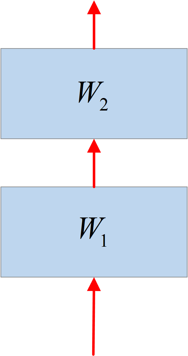
With this idea, review Eq.(6): the network is stacked by $W_{i}$, which means the network is built up layer by layer. Also, we can clearly see that there is only one path from the output of $layer_{L-i}$ to the output of $layer_{L}$ — go through $layer_{L-i+1}$, $layer_{L-i+2}$, …, till $layer_{L}$ as Figure 2(a).

(a) old CNNs

(b) residual networks $\left(1+W_{1}\right)\left(1+W_{2}\right)=1+W_{1}+W_{2}+W_{1}W_{2}$

Figure 2: Propagation paths in networks(red lines represent optional paths)

3.2 Analysis of Residual Networks

For the residual networks, the recursion formula is[2, 3]:

$$X_{i}=g_{i}\left[X_{i-1}+F\left(X_{i-1},\theta_{i}\right)\right],0<i<L+1$$ (7)

where $L$ is the total number of blocks.

Similarly, in order to make the propagation paths in the network easy to understand[3], we take the partial derivative of the output of the last block with respect to the output of a previous block and get the following fomula:

$$\frac{\partial X_{L}}{\partial X_{L-i}} =\frac{\partial X_{L}}{\partial X_{L-1}}\cdot\frac{\partial X_{L-1}}{\partial X_{L-2}}\cdot\ldots\cdot\frac{\partial X_{L-i+1}}{\partial X_{L-i}}$$ (8)

$$=g_{L}^{\prime}\left(1+W_{L}\right)\cdot g_{L-1}^{\prime}\left(1+W_{L-1}\right)\cdot\ldots\cdot g_{L-i+1}^{\prime}\left(1+W_{L-i+1}\right)$$ (9)

The new view of residual networks

To make a better comprehension of the architecture of the network, ignore the activation function in the Eq.(9) (activation function does not affect the architecture of a network):

$$\frac{\partial X_{L}}{\partial X_{L-i}} =\left(1+W_{L}\right)\left(1+W_{L-1}\right)\cdot\ldots\cdot\left(1+W_{L-i+1}\right)$$ (10)

$$=1+\mathrm{S}_{i}^{1}W+\mathrm{S}_{i}^{2}W+\ldots+\mathrm{S}_{i}^{i-2}W+\mathrm{S}_{i}^{i-1}W+\mathrm{S}_{i}^{i}W$$ (11)

$\mathrm{S}_{i}^{k}W$ represents all combinations that any k terms selected from $W$ to multiply, where $W=\left(W_{L},W_{L-1},W_{L-2},\ldots,W_{L-i+1}\right)$. For example, $\mathrm{S}_{3}^{2}({W}_{L},{W}_{L-1},{W}_{L-2})={W}_{L}\cdot{W}_{L-1}+{W}_{L}\cdot{W}_{L-2}+{W}_{L-1}\cdot{W}_{L-2}$.

Similarly to section 3.1, according to Eq.(10), we know that ResNets are stacked by $1+W_{i}$, which means the basic unit of ResNets consists of a shortcut and some sequence of convolutions.

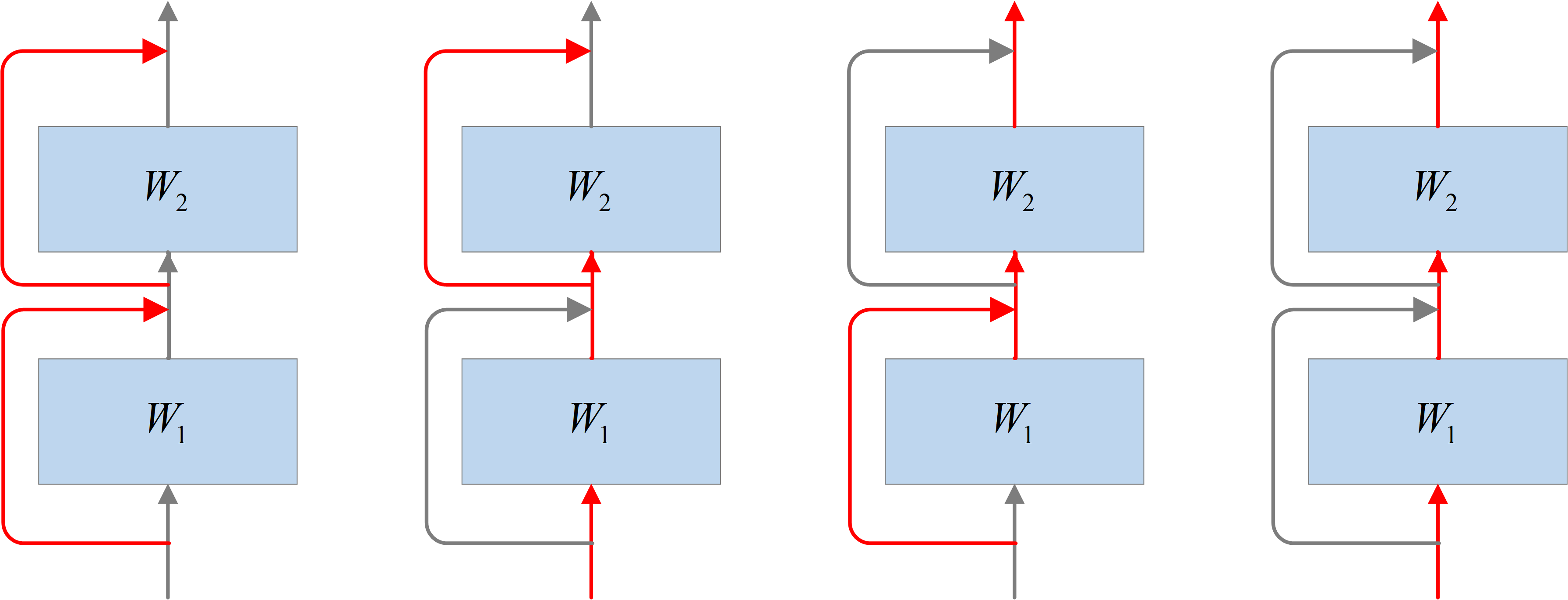
In Eq.(11), addition means parallel connection and multiplication means series connection. And, each multiplication term represents a path. For example, in $({W}_{L}\cdot{W}_{L-1}+{W}_{L}\cdot{W}_{L-2}+{W}_{L-1}\cdot{W}_{L-2})$, there are three paths that go through two blocks, which are ${W}_{L}\cdot{W}_{L-1}$, ${W}_{L}\cdot{W}_{L-2}$ and ${W}_{L-1}\cdot{W}_{L-2}$.

So, according to Eq.(11) and the definition of $\mathrm{S}_{i}^{k}W$, we can clearly see the propagation paths from the output of $block_{L-i}$ to the output of $block_{L}$ as Figure 2(b):
There is one path from ${block}_{L-i}$ straight to ${block}_{L}$
There are $\mathrm{C}_{1}^{i}$ paths from ${block}_{L-i}$ to ${block}_{L}$ through 1 block
There are $\mathrm{C}_{2}^{i}$ paths from ${block}_{L-i}$ to ${block}_{L}$ through 2 blocks
…
There are $\mathrm{C}_{i-1}^{i}$ paths from ${block}_{L-i}$ to ${block}_{L}$ through $i-1$ blocks
There is $\mathrm{C}_{i}^{i}$ path from ${block}_{L-i}$ to ${block}_{L}$ through $i$ blocks
where $C_{k}^{i}=\frac{i!}{k!(i-k)!}$, and $!$ represents factorial.

4 Method

According to section 3, by the comparison , the biggest difference between residual networks and the previous networks is the recursion formula — It is the small change of "+ 1" in the recursion formula that makes the entire network more powerful by recursion and multiplication.

Inspired by this, the architecture design of a network can start with the recursion formulas. Thus, we can study the properties of the network from the math nature, and explore better network architectures and more possibilities. Architectures designed in this way will be more interpretable in math.

The ultimate goal is the expected recursion formulas. There may be various ways to get them. Two ways to design new architectures are provided here:

Start with general formulas

By the analysis of section 3.1 and 3.2, it can be found that general formulas reflect the propagation paths in the network. Thus, if we want to change or design propagation paths from the perspective of the whole network, we can start with the general formulas like Eq.(6), Eq.(9) or $X_{L}=F\left(X_{L},X_{L-1},X_{L-2},\ldots,X_{0}\right)$, etc , $F$ is the expected function. According to the designed general formulas, the recursion formulas can be obtained. Then, the new architecture can be designed. The flow chart of this method is shown as Figure 1.

Start with recursion formulas

Recursion formulas represents the basic units in the network, which reflect the basic architecture of the network and the mapping relationship between the input and output of the basic units. Thus, if we want a certain basic architecture or mapping relationship like $X_{i}=F\left(X_{i},X_{i-1},X_{i-2},\ldots\right)$ or $X_{i}=F\left(W_{i}\right)\cdot X_{i-1}$, etc, we can directly start with recursion formulas, based on which the new architecture can be designed. The flow chart of this method is shown as Figure 1.

5 Example

5.1 Get the recursion formulas

According to section 3.1, consider the following problems[10] in ResNet: ResNet tends to take the shorter paths during training. Pathways of the same length have different widths and different expressive power. Too many optional paths will cause redundancy.

In terms of the above problems, we make some modifications to the Eq.(10):

$$\frac{\partial X_{L}}{\partial X_{L-i}}=1+\mathrm{W}_{L}+\mathrm{W}_{L}\cdot\mathrm{W}_{L-1}+\ldots+\mathrm{W}_{L}\cdot\mathrm{W}_{L-1}\cdot...\cdot\mathrm{W}_{L-i+1}$$ (12)

$$where\quad 0<i<L.$$

Eq.(12) guarantees that there is only one path per length from $X_{L-i}$ to $X_{L}$, which alleviates the redundancy. Besides, paths go through the the widest blocks ${W}_{L}\cdot{W}_{L-1}\cdot\ldots\cdot{W}_{L-i+1}$(for ${W}_{i}$, the larger $i$, the wider ${block}_{i}$), which ensures that the paths have the strongest expressive power. From ${W}_{L}\cdot{W}_{L-1}\cdot\ldots\cdot{W}_{L-i+1}$, it can also be found that longer paths are based on shorter paths.

For convenience, let:

$$\frac{\partial X_{L}}{\partial X_{L-i}}=f_{L-i}$$ (13)

Bring $\frac{\partial X_{L}}{\partial X_{L-i}}=f_{L-i}$ into Eq.(12), then we can get the recursion formula from them:

$$f_{L-i} =f_{L-i+1}+W_{L-i+1}\cdot\left(f_{L-i+1}-f_{L-i+2}\right)$$

$$=\left(1+W_{L-i+1}\right)\cdot f_{L-i+1}-W_{L-i+1}\cdot f_{L-i+2}$$ (14)

$$where\quad 1<i<L+1.$$

In Eq.(14), it can be seen that the output of the $(L-i)$-th block is not only related to the $(L-i+1)$-th block, but also related to the $(L-i+2)$-th block. This gives the basic block a memory capacity.

Then, bring $f_{L-i}=\frac{\partial X_{L}}{\partial X_{L-i}}$ into Eq.(14):

$$\frac{\partial X_{L}}{\partial X_{L-i}}=\left(1+W_{L-i+1}\right)\cdot\frac{\partial X_{L}}{\partial X_{L-i+1}}-W_{L-i+1}\cdot\frac{\partial X_{L}}{\partial X_{L-i+2}}$$ (15)

$$where\quad 1<i<L+1$$

An important method to further derive the partial derivative formula is the chain rule. Eq.(15) is supposed to be in the form of chain rule like Eq.(16), so that it makes sense:

$$\frac{\partial X_{L}}{\partial X_{L-i}} =\frac{\partial X_{L}}{\partial X_{L-i+2}}\frac{\partial X_{L-i+2}}{\partial X_{L-i}}$$ (16)

Eq.(15) can be regarded as the derivation from Eq.(16) or the expanded form of Eq.(16). Make them equal and we can get the following equtaion:

$$\frac{\partial X_{L-i+2}}{\partial X_{L-i}}=\left(1+\mathrm{W}_{L-i+1}\right)\frac{\partial X_{L-i+2}}{\partial X_{L-i+1}}-\mathrm{W}_{L-i+1}$$ (17)

According to Eq.(17), the inferences that $\frac{\partial X_{L-i+1}}{\partial X_{L-i}}=1+\mathrm{W}_{L-i+1}$ and $X_{L-i+2}$ consists of the term of ($-{W}_{L-i+1}\cdot X_{L-i}$) can be further obtained. Based on the inferences, we can get the following recursion formulas, which are good demonstration of the relationship between the blocks in the network and make it easy to learn about the overall architecture of the network:

$$X_{L}=\left(1+\mathrm{W}_{L}\right)\cdot X_{L-1}-\mathrm{W}_{L-1}\cdot X_{L-2}$$ (18)

$$X_{L-1}=\left(1+\mathrm{W}_{L-1}\right)\cdot X_{L-2}-\mathrm{W}_{L-2}\cdot X_{L-3}$$ (19)

$$...$$

$$X_{L-i}=\left(1+\mathrm{W}_{L-i}\right)\cdot X_{L-i-1}-\mathrm{W}_{L-i-1}\cdot X_{L-i-2}$$ (20)

$$where\quad 0<i<L-1$$

$$...$$

$$X_{1}=\left(1+\mathrm{W}_{1}\right)\cdot X_{0}$$

5.2 Design the architecture

According to the Eq.(20), it is easy to find that the equation has two parts:$\left(1+W_{L-i+1}\right)\cdot f_{L-i+1}$ which is the same as ResNet and $W_{L-i+1}\cdot f_{L-i+2}$ which is the output of the convolutional sequences in the previous block. We can design the architecture of the network as Figure 3. This example starts with general formulas that we want. Then, according to the general formulas, we get new recursion formulas, based on which we design the new architecture.

Figure 3: The newly designed architecture

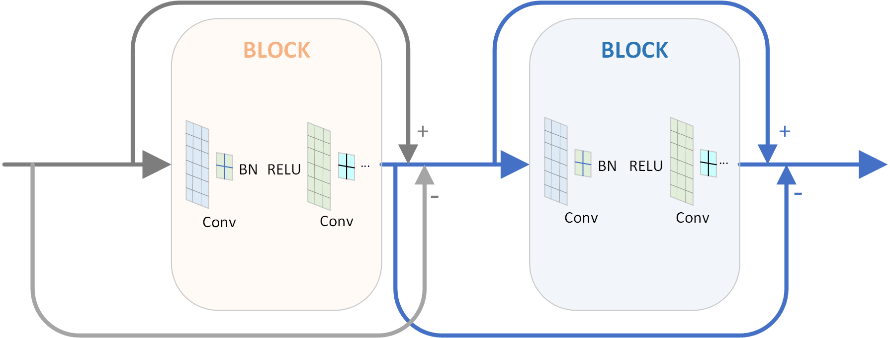
Note that the architecture must be designed according to recursion formulas like Eq.(20). Only in this way can the designed architecture has the expected propagation paths. Considering $X_{1}=\left(1+\mathrm{W}_{1}\right)X_{0}$ and the Eq.(20), if $X_{1}=\left(1+\mathrm{W}_{1}\right)X_{0}$ is brought into the recursion formulas, Eq.(18)-(20) will change into the following form:

$$X_{q}=W_{q}X_{q-1}+X_{0}$$ (21)

$$where\quad 1<q<L+1$$

Although, when $X_{1}=\left(1+\mathrm{W}_{1}\right)X_{0}$ is given, Eq.(18)-(20) and Eq.(21) are equivalent. The architectures designed according to them are quite different. And it can be found that if the architecture is designed according to Eq.(21), the output of the previous block cannot directly propagate to the next block and only the input of the network can propagate across layers, which is not in line with our idea. In addition, architectures designed by Eq.(20) and Eq.(21) have quite different performance in experiments. The latter perform much worse — slower convergence and worse accuracy.

The propagation paths should be emphasized in the design process. So, the network architecture is supposed to be designed according to the original recursion formulas , rather than the recursion formulas after the initial values are brought in.

5.3 Experiment

In this section, names plus $s$ of the networks denote corresponding networks with the new architecture. GPUs used are four TITAN RTXs. The complete experimental data obtained by using different random seeds is given in the appendix A.2.

5.3.1 Comparison with ResNet

The performances of ResNet18/34/50/101[2] and the corresponding networks with the new architecture are compared on the test sets. Because the new architecture is designed on the basis of ResNet, the hyperparameters of the corresponding networks are completely consistent.

On CIFAR data sets, all the networks are trained with momentum stochastic gradient descent[24] optimizer with a learning rate of 0.1, momentum of 0.9, and the weight decay $5\times 10^{-4}$. Besides, the scheduler used is cosine annealing[25] , the number of training epoch is 200 and batch size is 128.

On ImageNet data set, all the networks are trained with momentum stochastic gradient descent[24] optimizer with a learning rate of 0.1, momentum of 0.9, and weight decay $5\times 10^{-4}$. Besides, the scheduler used is MultiStepLR, the learning rate decays by a factor of 10 every 30 epochs, the number of training epoch is 90 and batch size is 256.

Table 1 shows the results of ResNets and the corresponding networks with newly designed architecture in our experiments. The networks with newly designed architecture achieve better performance than ResNets. And there is a steady improvement in accuracy on different baselines. Restricting information to the paths with strongest expressive power does improve network performance.

Table 1: The results of the newly designed network on test sets

Method	CIFAR10		CIFAR100		ImageNet
	top-1(%)	top-5(%)	top-1(%)	top-5(%)	top-1(%)	top-5(%)
ResNet18	94.32	99.76	76.60	93.36	68.63	88.58
ResNet18s	94.70	99.80	76.57	93.41	68.51	88.41
ResNet34	94.75	99.78	77.09	93.27	72.14	90.42
ResNet34s	95.10	99.88	77.48	93.77	72.38	90.77
ResNet50	95.00	99.88	78.37	94.26	75.13	92.36
ResNet50s	95.29	99.85	78.65	94.32	75.40	92.52
ResNet101	94.89	99.83	77.67	93.79	76.51	92.96
ResNet101s	95.01	99.86	78.56	93.86	76.73	93.20

5.3.2 Friedman Test & Nemenyi Test

In order to verify the significance of the new architecture[26], we conduct Friedman test and Nemenyi test on the networks[26, 27, 28]. The specific principles of this method are in the appendix A.1.

According to the experimental data on CIFAR10, CIFAR100 and ImageNet, Friedman graph can be drawn as Figure 4, where the horizontal axis value represents the ranking. The horizontal line in the graph denotes the ranking of the accuracy of the corresponding model in vertical axis. The solid origin denotes the mean value of the ranking on different data sets.

Figure 4: Friedman graph

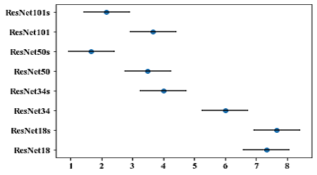
In the Friedman graph, if the two methods have no overlapping area, it proves that the performance of two methods is significantly different[26]. It can be seen that ResNet34/50/101 and ResNet34s/50s/101s have no overlapping area respectively. ResNet34s/50s/101s have better performance than ResNet34/50/101 on both CIFAR and ImageNet data sets. Also, it is easy to find that the performance of ResNet34s is comparable to that of ResNet50 and is better than that of ResNet101 on CIFAR data sets. The performance of ResNet50s far exceeds others on CIFAR data sets. It proves that the performance of the new architecture has been significantly improved compared to ResNet.

5.3.3 Further experiments

To validate the generality and compatibility of the proposed architecture with other popular neural networks, additional experiments are conducted with the 3 baselines: SEResNet[4], ResNeXt[6], Res2NeXt[7]. In table 2, ResNeXt2 and ResNeXt4 denote $ResNeXt29(2\times 64d)$ and $ResNeXt29(4\times 64d)$ respectively[6]. Res2NeXt2 and Res2NeXt4 denote $Res2NeXt29(6c\times 24w\times 4scales)$ and $Res2NeXt29(8c\times 25w\times 4scales)$ respectively[7].

Table 2: Results of other networks with the newly designed architecture

Method	CIFAR10	CIFAR100	Method	CIFAR10	CIFAR100
	top-1(%)	top-1(%)		top-1(%)	top-1(%)
SEResNet18	95.29	78.71	SEResNet18s	95.47	78.65
SEResNet34	95.58	79.05	SEResNet34s	95.86	80.15
SEResNet50	95.57	79.30	SEResNet50s	95.85	80.36
SEResNet101	95.51	79.36	SEResNet101s	95.80	80.09
ResNeXt2	95.67	79.39	ResNeXt2s	95.55	79.49
ResNeXt4	96.53	80.99	ResNeXt4s	96.53	81.06
Res2NeXt2	95.75	81.14	Res2NeXt2s	96.43	82.22
Res2NeXt4	96.16	79.27	Res2NeXt4s	96.09	82.49

Table 3: Comparison on ImageNet

Method	ImageNet	Method	ImageNet
	top-1(%)		top-1(%)
SEResNet34	68.624	SEResNet34s	69.182
SEResNet50	71.532	SEResNet50s	72.436
ResNeXt2	67.591	ResNeXt2s	68.412
ResNeXt4	72.390	ResNeXt4s	73.264

Table 2 gives the results of networks that take ResNet and the new architecture as architecture respectively. The newly designed architecture comprehensively improves the performance of SEResNet networks, which shows that the new architecture has a good compatibility with the attention mechanism. Through the comparison between ResNeXt/Res2NeXt and ResNeXts/Res2NeXts, the new architecture can achieve better training effect when the model is complex and difficult to train. At the same time, the new architecture tends to achieve better performance on complex tasks.

From another perspective, this architecture increases the average width of paths in each length, which also proves the importance of network width. We can come to a conclusion that appropriate increase in width can improve network performance [29, 30].

5.3.4 Experiment summary

In this example, additional cross-layer connections will increase the number of parameters[2]. We do not focus on reducing the model size in this example since what we want to show is the design process and design ideas. The model sizes and computational complexity are given in appendix A.3. On the one hand, this example can be considered as architecture optimization, which picks out the paths with the strongest expressive power and increases the average width of each length path; on the other hand, this example can be considered as a method that increases the number of network parameters to stably improves the network performance by additional cross-layer connections while keeping the network depth and feature map channels unchanged.

6 Conclusion

In this paper, we show the effect of recursion formulas on network architectures and show the propagation paths in networks by taking the partial derivative of the output of the last block/layer with respect to the output of a previous block/layer. In the meanwhile, a mathematical method to design network architectures is proposed. Based on the method, a new architecture is designed as an example. The entire design process shows how the theory guides the experiment. Comparative experiments are conducted on CIFAR and ImageNet, which shows that the network with the newly designed architecture has better performance than ResNet and the newly designed architecture has the generality and compatibility with other popular neural networks. This verifies the feasibility of the proposed method.

7 Future Work and Broader Impact

Future work

This work is an attempt to design the network architecture completely from the perspective of mathematical formulas. In the future, we will continue to improve the theoretical system of using mathematics to solve neural network problems. We hope that through our efforts, we can make the related research of artificial intelligence more mathematical and theoretical, rather than relying more on genius inspiration and a large number of experimental trial and error. Mathematical theory, physical theory and information theory are all great treasures, and they all have a solid theoretical foundation. The analysis methods in these fields can be used for reference. The development of artificial intelligence should not be independent of them, but should be integrated with them.

Broader impact

We analyze the architectures of networks and propagation paths in networks by mathematical formulas, which makes the network architecture more interpretable and easier to understand. This method to design architectures of networks makes the design of the network architecture have a mathematical theoretical basis. This promotes the combination of network architecture design and mathematics. This may also promote the emergence of more new network architectures in the future. The negative outcomes result from the increasing accuracy of image recognition and more used surveillance cameras. That may raise the risk of privacy breaches and other security issues, which may put everyone under monitoring.

Appendix A Appendix

A.1 Friedman test and Nemenyi test

For $k$ algorithms and $N$ data sets, first get the test performance results of each algorithm on each data set, and then sort them according to the performance results from good to bad, and give the order value $1,2,…,k$. If the performance results of multiple algorithms are the same, they are equally divided into rank values. Assuming the average rank value of the $i$-th algorithm is ${r}_{i}$, then ${r}_{i}$ obeys the normal distribution:

$$\tau_{x^{2}}=\frac{12N}{k(k-1)}\left(\sum_{i=1}^{k}r_{i}^{2}-\frac{k(k+1)^{2}}{4}\right)$$

$$\tau_{\mathrm{F}}=\frac{(N-1)\tau_{x^{2}}}{N(k-1)-\tau_{x^{2}}}$$

where, $\tau_{F}$ Obey the $F$ distribution with degrees of freedom $k-1$ and $(k-1)(N-1)$.

If the hypothesis of "all algorithms have the same performance" is rejected, it means that the performance of the algorithms is significantly different, and then a follow-up test is required.

The Nemenyi test calculates the critical value range $CD$ of the average ordinal difference:

$$CD=q_{\alpha}\sqrt{\frac{k(k+1)}{6N}}$$

The $q_{\alpha}$ values are listed in the table 4.

Table 4: $q_{\alpha}$ values

$\alpha$	k algorithms
	2	3	4	5	6	7	8	9	10
0.05	1.960	2.334	2.569	2.728	2.850	2.949	3.031	3.102	3.164
0.10	1.645	2.052	2.291	2.459	2.589	2.693	2.780	2.855	2.920

If the rank value difference of any two algorithms is bigger than $CD$, there is a significant difference in performance of the two algorithms.

A.2 Experiment Datas

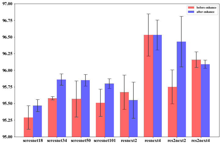
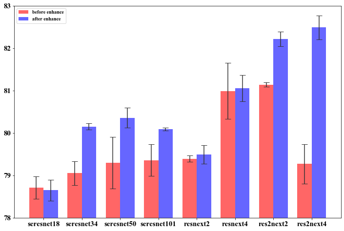
The complete experiment data mentioned in section 5.3.3 is in table 5, table 6 and table 7. The histograms with error bars are in Figure 5 and Figure 6. Complete data on ImageNet is being collected.

Table 5: Seed = 0

Method	CIFAR10	CIFAR100	Method	CIFAR10	CIFAR100
	top-1(%)	top-1(%)		top-1(%)	top-1(%)
SEResNet18	95.42	79.01	SEResNet18s	95.54	78.91
SEResNet34	95.62	79.34	SEResNet34s	95.91	80.05
SEResNet50	95.52	80.10	SEResNet50s	95.83	80.65
SEResNet101	95.42	79.09	SEResNet101s	95.79	80.09
ResNeXt2	95.98	79.31	ResNeXt2s	95.90	79.72
ResNeXt4	96.36	81.59	ResNeXt4s	96.44	81.45
Res2NeXt2	95.40	81.14	Res2NeXt2s	96.16	82.43
Res2NeXt4	96.32	78.66	Res2NeXt4s	96.02	82.09

Table 6: Seed = 617

Method	CIFAR10	CIFAR100	Method	CIFAR10	CIFAR100
	top-1(%)	top-1(%)		top-1(%)	top-1(%)
SEResNet18	95.02	78.37	SEResNet18s	95.34	78.73
SEResNet34	95.56	78.67	SEResNet34s	95.74	80.21
SEResNet50	95.27	79.19	SEResNet50s	95.76	80.06
SEResNet101	95.31	79.88	SEResNet101s	95.72	80.13
ResNeXt2	95.67	79.49	ResNeXt2s	95.24	79.55
ResNeXt4	96.25	80.23	ResNeXt4s	96.31	80.69
Res2NeXt2	96.01	81.07	Res2NeXt2s	96.17	82.22
Res2NeXt4	96.12	79.79	Res2NeXt4s	96.08	82.66

Table 7: Seed = 1234

Method	CIFAR10	CIFAR100	Method	CIFAR10	CIFAR100
	top-1(%)	top-1(%)		top-1(%)	top-1(%)
SEResNet18	95.37	78.76	SEResNet18s	95.52	78.32
SEResNet34	95.57	79.15	SEResNet34s	95.93	80.20
SEResNet50	95.93	78.62	SEResNet50s	95.97	80.36
SEResNet101	95.79	79.10	SEResNet101s	95.90	80.06
ResNeXt2	95.35	79.37	ResNeXt2s	95.52	79.20
ResNeXt4	96.97	81.15	ResNeXt4s	96.84	81.06
Res2NeXt2	95.83	81.20	Res2NeXt2s	96.97	82.01
Res2NeXt4	96.04	79.36	Res2NeXt4s	95.93	82.71

Figure 5: CIFAR10

Figure 6: CIFAR100

A.3 Params of models

Table 8: FLOPs and model size on CIFAR100

Model	FLOPs	Params	Acc(%)	Model	FLOPs	Params	Acc(%)
ResNet18	$7.1\times 10^{10}$	11.22M	76.60	ResNet18s	$7.2\times 10^{10}$	11.39M	76.57
ResNet34	$1.5\times 10^{11}$	21.33M	77.09	ResNet34s	$1.5\times 10^{11}$	21.50M	77.48
ResNet50	$1.7\times 10^{11}$	23.70M	78.37	ResNet50s	$1.8\times 10^{11}$	26.48M	78.65
ResNet101	$3.2\times 10^{11}$	42.70M	77.67	ResNet101s	$3.4\times 10^{11}$	45.47M	78.56
SEResNet18	$7.1\times 10^{10}$	11.31M	78.71	SEResNet18s	$7.2\times 10^{10}$	11.48M	78.65
SEResNet34	$1.5\times 10^{11}$	21.50M	79.05	SEResNet34s	$1.5\times 10^{11}$	21.67M	80.15
SEResNet50	$1.7\times 10^{11}$	26.26M	79.30	SEResNet50s	$1.8\times 10^{11}$	29.04M	80.36
SEResNet101	$3.2\times 10^{11}$	47.53M	79.36	SEResNet101s	$3.4\times 10^{11}$	50.31M	80.09
ResNeXt2	$1.8\times 10^{11}$	9.22M	79.39	ResNeXt2s	$1.9\times 10^{11}$	9.89M	79.49
ResNeXt4	$5.4\times 10^{11}$	27.29M	80.99	ResNeXt4s	$5.8\times 10^{11}$	29.95M	81.06
Res2NeXt2	$6.1\times 10^{11}$	33.10M	81.14	Res2NeXt2s	$6.3\times 10^{11}$	34.61M	82.22
Res2NeXt4	$8.7\times 10^{11}$	47.27M	79.27	Res2NeXt4s	$8.9\times 10^{11}$	48.91M	82.49

In table 8, ResNeXt2 and ResNeXt4 denote $ResNeXt29(2\times 64d)$ and $ResNeXt29(4\times 64d)$ respectively. Res2NeXt2 and Res2NeXt4 denote $Res2NeXt29(6c\times 24w\times 4scales)$ and $Res2NeXt29(8c\times 25w\times 4scales)$ respectively.

It can be found that there is no significant difference in the computational complexity between the enhanced model and the baseline model. The accuracy of multiple networks with the new architecture has a stable improvement.

A.4 additional examples

Start with recursion formulas

The recursion formulas of residual networks and the traditional CNNs are in the following form:

$$X_{i}=F\left(X_{i-1},\theta_{i}\right)$$

where $X_{i-1}$ and $X_{i}$ denote the input and output of the $i$-th block/layer, $\theta_{i}$ denotes the parameters of the $i$-th block/layer. According to the above equation, the output of the current block/layer is only related to the output of the previous block/layer.

A.4.1 additional example 1

Consider the following form of recursion formulas:

$$X_{i}=F\left(X_{i-1},X_{i-2},\theta_{i}\right)=W_{i}\cdot X_{i-1}+X_{i-2}$$

where $W$ denotes the mapping of the block/layer and $1<i<L+1$. Based on the recursion formula, a new architecture can be designed as Figure 7.

Figure 7: The architecture of additional example 1

A.4.2 additional example 2

Consider the following form of recursion formulas:

$$X_{i}=F\left(X_{i-1},X_{i-2},\theta_{i},\theta_{i-1}\right)$$

We can design a recursion formula that fits this form as follows:

$$X_{i}=F\left(X_{i-1},\theta_{i}\right)+F\left(X_{i-2},\theta_{i-1}\right)=W_{i}\cdot X_{i-1}+W_{i-1}\cdot X_{i-2}$$

where $W$ denotes the mapping of the block/layer and $1<i<L+1$. Based on the recursion formula, a new architecture can be designed as Figure 8.

Figure 8: The architecture of additional example 2

A.5 Pytorch Code

Here is the Pytorch code of the example in section 5

A.5.1 Code of the basic block

def forward(self, x): out = F.relu(self.bn1(self.conv1(x[1]))) out = self.bn2(self.conv2(out)) outp = out out += self.shortcut(x[1]) out = F.relu(out) out -= self.shortcut2(x[0]) out = torch.stack((outp, out)) return out

A.5.2 Code of the bottleneck

def forward(self, x): out = F.relu(self.bn1(self.conv1(x[1]))) out = F.relu(self.bn2(self.conv2(out))) out = self.bn3(self.conv3(out)) outp = out out += self.shortcut(x[1]) out = F.relu(out) out -= self.shortcut2(x[0]) out = torch.stack((outp, out)) return out

A.6 Reproduction details

CIFAR

The input size is $32\times 32$. All the networks are trained with momentum stochastic gradient descent optimizer with a learning rate of 0.1, momentum of 0.9, and the weight decay $5\times 10^{-4}$. Besides, the scheduler used is cosine annealing , the number of training epoch is 200 and batch size is 128.

ImageNet

The input size is $224\times 224$. All the networks are trained with momentum stochastic gradient descent optimizer with a learning rate of 0.1, momentum of 0.9, and weight decay $5\times 10^{-4}$. Besides, the scheduler used is MultiStepLR, the learning rate decays by a factor of 10 every 30 epochs, the number of training epoch is 90 and batch size is 256.

Baselines

We do not use any improvement methods, such as label smoothing, etc. The hyperparameters of the baseline models on the CIFAR and ImageNet are a little different.

Table 9: Baseline details on different data sets

Dataset	Pre	Layer1	Layer2	Layer3	Layer4	Last
CIFAR	3c, $3\times 3$, 64c	64c, 64c	64c, 128c	128c, 256c	256c, 512c	avg-pool(4), fc
ImageNet	3c, $7\times 7$, 64c	64c, 64c	64c, 128c	128c, 256c	256c, 512c	avg-pool(7), fc

Table 9 shows the hyperparameters on different data sets, where Layer denotes the unit that contains multiple blocks, c denotes channels, $3\times 3$ and $7\times 7$ denote convolution kernel size and fc denotes full connection layer. How many blocks Layer1, Layer2, Layer3 and Layer4 contain determines the number of layers in the network.

And we complete our code with reference to the following open source code:
https://github.com/bearpaw/pytorch-classification with MIT license
https://github.com/Res2Net/Res2Net-PretrainedModels
https://github.com/jiweibo/ImageNet with MIT license
https://github.com/kuangliu/pytorch-cifar with MIT license

References

- [1] Srivastava, R. K., Greff, K., & Schmidhuber, J. (2015). Highway networks. arXiv preprint arXiv:1505.00387.
- [2] He, K., Zhang, X., Ren, S., & Sun, J. (2016). Deep residual learning for image recognition. In Proceedings of the IEEE conference on computer vision and pattern recognition (pp. 770-778).
- [3] He, K., Zhang, X., Ren, S., & Sun, J. (2016, October). Identity mappings in deep residual networks. In European conference on computer vision (pp. 630-645). Springer, Cham.
- [4] Hu, J., Shen, L., & Sun, G. (2018). Squeeze-and-excitation networks. In Proceedings of the IEEE conference on computer vision and pattern recognition (pp. 7132-7141).
- [5] Huang, G., Liu, Z., Van Der Maaten, L., & Weinberger, K. Q. (2017). Densely connected convolutional networks. In Proceedings of the IEEE conference on computer vision and pattern recognition (pp. 4700-4708).
- [6] Xie, S., Girshick, R., Dollár, P., Tu, Z., & He, K. (2017). Aggregated residual transformations for deep neural networks. In Proceedings of the IEEE conference on computer vision and pattern recognition (pp. 1492-1500).
- [7] Gao, S., Cheng, M. M., Zhao, K., Zhang, X. Y., Yang, M. H., & Torr, P. H. (2019). Res2net: A new multi-scale architecture architecture. IEEE transactions on pattern analysis and machine intelligence.
- [8] Tan, M., & Le, Q. (2019, May). Efficientnet: Rethinking model scaling for convolutional neural networks. In International Conference on Machine Learning (pp. 6105-6114). PMLR.
- [9] Zamir, A. R., Wu, T. L., Sun, L., Shen, W. B., Shi, B. E., Malik, J., & Savarese, S. (2017). Feedback networks. In Proceedings of the IEEE conference on computer vision and pattern recognition (pp. 1308-1317).
- [10] Veit, A., Wilber, M., & Belongie, S. (2016). Veit, A., Wilber, M., & Belongie, S. (2016, December). Residual networks behave like ensembles of relatively shallow networks. In Proceedings of the 30th International Conference on Neural Information Processing Systems (pp. 550-558).
- [11] Bello, I., Fedus, W., Du, X., Cubuk, E. D., Srinivas, A., Lin, T. Y., … & Zoph, B. (2021). Revisiting ResNets: Improved training and scaling strategies. arXiv preprint arXiv:2103.07579.
- [12] Wu, Z., Shen, C., & Van Den Hengel, A. (2019). Wider or deeper: Revisiting the ResNet model for visual recognition. Pattern Recognition, 90, 119-133.
- [13] Krizhevsky, A., & Hinton, G. (2009). Learning multiple layers of features from tiny images.
- [14] Krizhevsky, A., Sutskever, I., & Hinton, G. E. (2012). Imagenet classification with deep convolutional neural networks. Advances in neural information processing systems, 25, 1097-1105.
- [15] LeCun, Y., Bottou, L., Bengio, Y., & Haffner, P. (1998). Gradient-based learning applied to document recognition. Proceedings of the IEEE, 86(11), 2278-2324.
- [16] Hochreiter, S., & Schmidhuber, J. (1997). Long short-term memory. Neural computation, 9(8), 1735-1780.
- [17] Howard, A. G., Zhu, M., Chen, B., Kalenichenko, D., Wang, W., Weyand, T., … & Adam, H. (2017). Mobilenets: Efficient convolutional neural networks for mobile vision applications. arXiv preprint arXiv:1704.04861.
- [18] Sandler, M., Howard, A., Zhu, M., Zhmoginov, A., & Chen, L. C. (2018). Mobilenetv2: Inverted residuals and linear bottlenecks. In Proceedings of the IEEE conference on computer vision and pattern recognition (pp. 4510-4520).
- [19] Zhang, X., Zhou, X., Lin, M., & Sun, J. (2018). Shufflenet: An extremely efficient convolutional neural network for mobile devices. In Proceedings of the IEEE conference on computer vision and pattern recognition (pp. 6848-6856).
- [20] Ma, N., Zhang, X., Zheng, H. T., & Sun, J. (2018). Shufflenet v2: Practical guidelines for efficient cnn architecture design. In Proceedings of the European conference on computer vision (ECCV) (pp. 116-131).
- [21] Szegedy, C., Ioffe, S., Vanhoucke, V., & Alemi, A. (2017, February). Inception-v4, inception-resnet and the impact of residual connections on learning. In Proceedings of the AAAI Conference on Artificial Intelligence (Vol. 31, No. 1).
- [22] Szegedy, C., Liu, W., Jia, Y., Sermanet, P., Reed, S., Anguelov, D., … & Rabinovich, A. (2015). Going deeper with convolutions. In Proceedings of the IEEE conference on computer vision and pattern recognition (pp. 1-9).
- [23] Szegedy, C., Vanhoucke, V., Ioffe, S., Shlens, J., & Wojna, Z. (2016). Rethinking the inception architecture for computer vision. In Proceedings of the IEEE conference on computer vision and pattern recognition (pp. 2818-2826).
- [24] Sutskever, I., Martens, J., Dahl, G., & Hinton, G. (2013, May). On the importance of initialization and momentum in deep learning. In International conference on machine learning (pp. 1139-1147). PMLR.
- [25] Loshchilov, I., & Hutter, F. (2016). Sgdr: Stochastic gradient descent with warm restarts. arXiv preprint arXiv:1608.03983.
- [26] Demšar, J. (2006). Statistical comparisons of classifiers over multiple data sets. The Journal of Machine Learning Research, 7, 1-30.
- [27] Friedman, M. (1937). The use of ranks to avoid the assumption of normality implicit in the analysis of variance. Journal of the american statistical association, 32(200), 675-701.
- [28] Lin, Y., Hu, Q., Liu, J., Li, J., & Wu, X. (2017). Streaming feature selection for multilabel learning based on fuzzy mutual information. IEEE Transactions on Fuzzy Systems, 25(6), 1491-1507.
- [29] Wu, Z., Shen, C., & Van Den Hengel, A. (2019). Wider or deeper: Revisiting the resnet model for visual recognition. Pattern Recognition, 90, 119-133.
- [30] Nguyen, T., Raghu, M., & Kornblith, S. (2020). Do Wide and Deep Networks Learn the Same Things? Uncovering How Neural Network Representations Vary with Width and Depth. arXiv preprint arXiv:2010.15327.