GeoCLR: Georeference Contrastive Learning for Efficient Seafloor Image Interpretation
Abstract
This paper describes Georeference Contrastive Learning of visual Representation (GeoCLR) for efficient training of deep-learning Convolutional Neural Networks (CNNs). The method leverages georeference information by generating a similar image pair using images taken of nearby locations, and contrasting these with an image pair that is far apart. The underlying assumption is that images gathered within a close distance are more likely to have similar visual appearance, where this can be reasonably satisfied in seafloor robotic imaging applications where image footprints are limited to edge lengths of a few metres and are taken so that they overlap along a vehicle’s trajectory, whereas seafloor substrates and habitats have patch sizes that are far larger. A key advantage of this method is that it is self-supervised and does not require any human input for CNN training. The method is computationally efficient, where results can be generated between dives during multi-day AUV missions using computational resources that would be accessible during most oceanic field trials. We apply GeoCLR to habitat classification on a dataset that consists of ~86k images gathered using an Autonomous Underwater Vehicle (AUV). We demonstrate how the latent representations generated by GeoCLR can be used to efficiently guide human annotation efforts, where the semi-supervised framework improves classification accuracy by an average of 10.2 % compared to the state-of-the-art SimCLR using the same CNN and equivalent number of human annotations for training.
1 Introduction
Robotic imaging surveys can enable regional scale understanding of seafloor substrate and habitat distributions. Since visual images are limited to edge lengths of a few metres in water due to the strong attenuation of light, multiple overlapping georeferenced images need to be gathered to describe larger scale patterns that exist on the seafloor. Camera equipped Autonomous Underwater Vehicles (AUVs) achieve this by gathering tens of thousands of images during their dives at close and near-constant altitudes, with most AUV expeditions lasting many weeks and consisting of several deployments. However, taking advantage of the growing repositories of seafloor images is a challenge because our ability to interpret images cannot keep up with the influx of data.
Modern machine learning techniques have demonstrated robust, automated image interpretation. Much of the progress in this area has been driven by the availability of generic datasets consisting of over a million human labelled images to supervise the training of deep-learning convolutional neural networks (CNNs). In domains with high learning transferability, this allows deep-learning to be used in applications where the large amount of human effort required to generate labelled training data would be unjustified. However, the appearance of an underwater image is highly sensitive to the environment (e.g. seawater attenuation properties and turbidity), observation variables (e.g. range to target) and hardware choices (e.g. lighting and camera configurations), and these factors limit transferability of learning across datasets. This has so far limited large scale generic training datasets from being developed in this domain, and even if these were developed, it is still an open question as to whether these would be as effective as those used in terrestrial applications.
To address this issue, we investigate self-supervision techniques for deep-learning CNNs. Self-supervision is a subset of unsupervised learning, which generates optimised feature descriptors without using human annotations. Self-supervision aims to improve the quality of the image representation by using additional non-image, or image derived data that can be automatically associated with each image to constrain learning. A key advantage of these methods are that they can generate low-dimensional feature vectors on a per dataset basis, making them effective in domains where there is limited transferability of learning across datasets. Once the representations are obtained, various machine learning techniques such as clustering, content retrieval and few-shot learning can be efficiently applied. Contrastive learning is a form of self-supervision that has demonstrated robust performance gains across many application areas in the image representation learning domain [Chen et al., 2020, Jing and Tian, 2020, Le-Khac et al., 2020]. It works by giving similar and dissimilar image pairs to a CNN, optimising the representation that gets generated by mapping similar image pairs within a close distance in the latent representation space, and dissimilar image pairs so that they are separated in this space. To ensure images are similar without relying on human input, most contrastive learning techniques use data augmentation, i.e, applying random transformation to the same image to obtain similar but not identical pairs of images. In this work, we develop a novel method of Georeference enhanced Contrastive Learning for image Representation (GeoCLR), that leverages the 3D location information attached to each image to identify similar pairs of images in target dataset, making the assumption that physically close images are more likely to be similar in appearance than images taken at a larger spatial interval. This assumption is reasonable for the application considered in this work since AUV imagery is taken at close, often overlapping spatial intervals, and when describing substrates and habitats, the features of interest span or recur over spatial scales larger than the footprint of an individual image frame.
The contributions of this work are:
-
•
Development of GeoCLR, a novel contrastive representation learning technique for georeferenced seafloor imagery, leveraging an assumption that a pair of images taken physically close to each other are more likely to have similar appearance than a random pair when identifying similar and dissimilar image pairs in a dataset.
-
•
Development of an efficient method to use self-supervised learning outputs to guide human labelling effort to improve the accuracy of low-shot classification.
-
•
Experimental verification of the proposed method’s effectiveness through comparison with current state-of-the-art transfer learning and augmentation based contrastive learning, or SimCLR, techniques using a seafloor image dataset consisting of ~86k AUV images gathered over 12 dives with over ~5k human labels.
2 Background
2.1 Representation Learning for Seafloor Imagery
Visual images of the seafloor contain useful information for mapping substrate and habitat distribution. However, the high-dimensionality and redundant information in raw images is a challenge for classification. Therefore, most algorithmic interpretations first convert images to lower-dimensional representations, or feature spaces, that can be more efficiently analysed. Several types of feature descriptor have been investigated for seafloor image representations [Steinberg et al., 2011, Beijbom et al., 2012, Bewley et al., 2015, Kaeli and Singh, 2015, Rao et al., 2017, Neettiyath et al., 2020]. In [Beijbom et al., 2012, Neettiyath et al., 2020], colour descriptors are designed to target known targets of scientific interest, such as corals [Beijbom et al., 2012] and mineral deposits [Neettiyath et al., 2020]. Generic feature descriptors such as Local Binary Patterns (LBP) [Ojala et al., 2002] and Sparse Coding Spatial Pyramid Matching (ScSPM) [Yang et al., 2009] have also been applied to capture multi-scale spatially invariant patterns in seafloor images [Bewley et al., 2015, Rao et al., 2017]. In [Kaeli and Singh, 2015], histograms of oriented gradients from image keypoints are applied for clustering and anomaly detection. These approaches share common steps of selecting effective descriptors and parameter tuning, or feature engineering, that can be time consuming and require knowledge of how targets of interest are expected to appear in the images.
CNNs avoid the need for feature engineering by learning the representations needed to describe the datasets they are trained on. In supervised learning, this is achieved using human annotated examples in a training dataset, where the latent representations and class boundaries to best describe the patterns of interest are simultaneously optimised. In [Mahmood et al., 2018], the deep-learning CNN ResNet [He et al., 2016] is trained to classify nine different types of coral in a seafloor image dataset, demonstrating higher classification resolution and accuracy than traditional feature engineering methods. However, the need for large volumes of annotated images limits wide scale use in marine applications as generic training methods and datasets do not currently exist in this domain.
2.2 Self-supervised learning for Seafloor Imagery
An alternative approach to train CNNs is self-supervised learning using properties of the data that can be leveraged without the need for direct human supervision. Unlike state-of-the-art supervised training methods such transfer learning, where CNNs are pre-trained with large annotated datasets such as ImageNet [Deng et al., 2009], self-supervised methods train CNNs on the target dataset itself and so are effective in domains where there is a limited transferability of learning between the target dataset and those available for pre-training. In [Yamada et al., 2021b], a deep-learning convolutional autoencoder based on AlexNet [Krizhevsky et al., 2012] is used for representation learning of seafloor images. Autoencoders consist of an encoder and decoder pair, where the encoder maps the original data into low-dimensional latent representations. Next, the decoder reconstructs the original data from the low-dimensional latent representation, where both the encoder and decoder networks are optimised to make the reconstructed data as similar to the original input data as possible. This dimensional reduction attempts to remove redundant information in the raw inputs, retaining only the most important information in compact latent representations at the encoder output. In [Yamada et al., 2021b], the authors developed a Location Guided Autoencoder (LGA) that uses horizontal location information to regularise learning by leveraging the assumption that images captured at nearby locations are more likely to look similar than images that are far apart since seafloor habitats and substrates exhibit patterns larger than the footprint of a single image frame. The method significantly outperformed standard convolutional autoencoders without location regularisation, achieving a factor of 2 improvement in normalised mutual information when applied to clustering and content-based retrieval tasks. In [Yamada et al., 2021a], the LGA is extended to leverage other types of metadata, such as depth information, where the continuity in measurements have potential correlation with image appearance, where it was demonstrated that these terms can be included without risk of performance degradation through the design of a robust regularisation process.
2.3 Contrastive Learning Concepts for Image Representation
The recent development of contrastive learning concepts have demonstrated significant performance gains in self-supervised representation learning [Jing and Tian, 2020, Le-Khac et al., 2020]. The main idea behind contrastive concepts is to simultaneously provide similar and dissimilar image pairs during training, where similar pairs are mapped close to each other in the representation space, and dissimilar pairs are mapped far apart. These concepts require a binary prior that describes whether the image pairs provided during training are expected to be similar or not.
In [Chen et al., 2020], a method to generate similar and dissimilar pairs without any direct human input is developed using data augmentation. The proposed Simple framework for Contrastive Learning of visual Representations (SimCLR) applies random data augmentations to artificially generate similar image pairs, which are then contrasted with dissimilar pairs where different images are used. The method demonstrated significant gains in performance compared to supervised training using transfer learning approach [Tan et al., 2018].
3 Contrastive Representation Learning Leveraging Georeference Information
The use of location information to regularise autoencoder training can enhance the performance of seafloor image representation [Yamada et al., 2021b, Yamada et al., 2021a]. Here, we investigate whether georeference information can also be leveraged to improve the latent representations generated in contrastive learning [Chen et al., 2020]. Unlike the modified autoencoder loss functions used in our previous work where location information can be used to loosely regularise learning, the binary similarity condition that is imposed in contrastive learning forces a much stronger constraint on the latent representations that get generated. In order to validate this similarity assumption, we take advantage of the fact that AUVs capture images that often overlap and have footprints that are generally smaller than the patch size of habitats and substrates on the seafloor.
The following subsections give an overview of state-of-the-art modern contrastive learning approaches such as SimCLR [Chen et al., 2020], and introduce a novel Georeference Contrastive Learning of visual Representation (GeoCLR) method for efficient representation of spatially contiguous georeferenced imagery.
3.1 SimCLR
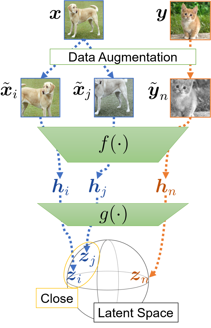
SimCLR learns representations by maximising agreement between differently augmented images generated from the same original image. The learning framework, illustrated in Figure 1(a), consists of four parts; data augmentation, base encoder , projection head and a contrastive loss function. Data augmentation transforms each image in the target dataset randomly to artificially generate two correlated images, and , where random cropping, colour distortions and Gaussian blur augmentations are applied in this order. The base encoder is a CNN that extracts representation vectors from the augmented images. The method allows any CNN to be used for , where [Chen et al., 2020] found this approach to be most effective on deeper and wider ResNet [He et al., 2016] architectures. is a feature vector extracted from by the base encoder (). The projection head is a two layer multilayer perceptron (MLP) to obtain (). The dimension of the MLP output are smaller than the dimension of the base encoder since the contrastive losses defined in lower-dimensional spaces are more efficient for representation learning. A minibatch of original images are taken into consideration at each iteration, so augmented images including similar pairs are sampled. For a similar pair, other augmented images ( in Figure 1(a)) can be regarded as dissimilar examples within the minibatch. The Normalised Temperature-scaled Cross Entropy loss function (NT-Xent) [Sohn, 2016, Wu et al., 2018, Oord et al., 2018] between the similar pair and is defined as
| (1) |
where sim() denotes cosine similarity, is the indicator function which is 1 if , and is the temperature parameter. The total minibatch loss can be written as,
| (2) |
The parameters of the base encoder and the projection head are updated by a stochastic gradient descent (SGD) optimiser with linear rate scaling [Goyal et al., 2017].
SimCLR can efficiently train CNNs using large unannotated image datasets, where the latent representations derived from the original images were shown to outperform other state-of-the-art methods in the benchmark classification tasks. It was further shown that fine-tuning of SimCLR trained CNNs can achieve more accurate classification with two orders of magnitude fewer labels than conventional supervised training methods.
3.2 GeoCLR
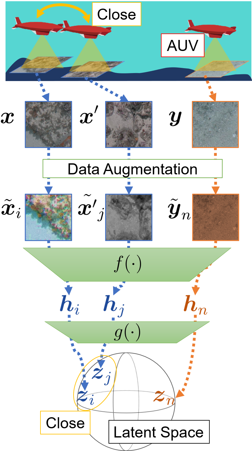
A limitation of SimCLR is that the variety of possible image appearances is limited by the types of augmentation used, and only features intrinsic to each image can be efficiently extracted. However, when applied to practical semantic interpretation, we are typically interested in correlating images that show a greater degree of variability than can be described by algorithmic augmentation alone. We predict that the performance of downstream interpretation tasks will benefit if a greater variety of appearances can be integrated into the similar pairs during CNN training. The GeoCLR method proposed in this paper allows great variability to be introduced into the similar image pairs by leveraging the georeference information associated with each image. We argue that the level of variability between images taken nearby will exhibit a level of variability that is more representative of that seen across similar habitats or substrates than augmentation alone.
Figure 1(b) shows the overview of GeoCLR. In GeoCLR, each similar image pair , is generated from two different images, where and are generated from , which is a different image to but is taken of a physically nearby location. For each image captured at the 3D georeference of , is randomly selected at each iteration from the images which satisfy the following criteria:
| (3) |
where is the 3D georeference of , is the scaling factor for depth direction. Introducing allows the depth difference between images to be weighted so that the nearby images with large depth gap are not selected, where values of tend to ignore differences in depth. This flexibility is introduced because the relative impact depth has on image appearance can vary across different application, where for example shallow water application typically have a stronger correlation due to the variable influence of sunlight reaching the seafloor than deep-sea applications. To identify an image pair, the distance needs to be larger than the distance between adjacent images taking into account variability in the acquisition interval, and smaller than the patch size of substrates and habitats so that paired images are likely to be similar in appearance. In practise, a small value is advantageous since the similarity assumption is likely to be violated near patch boundaries as increases. The lower limit for should also be conservatively set since restricting pairs to only its nearest neighbour means that the same pairing is more likely to be selected multiple times during training, which does not generate any additional information compared to the original SimCLR.
Once is selected, the same types of random data augmentation used in SimCLR are applied to each image to obtain the similar pair , .
4 Experiment
The proposed GeoCLR is applied to a dataset consisting of 86,772 georeferenced seafloor images obtained off the coast of Tasmania. The CNN is first trained on all images in the dataset to generate latent representations. Next, classification tasks are given to the trained CNN and the extracted features by the CNN, so that the performance can be evaluated based on classification accuracy. A variety of methods are used to train these classifiers, including the use of the latent representations to guide human annotation effort for efficient low-shot semi-supervised learning. The performance of the proposed GeoCLR, is evaluated through comparison with SimCLR and transfer learning under the equivalent conditions.
4.1 Dataset
| Vehicle | Sirius AUV |
|---|---|
| Camera Resolution | 1,360 1,024 |
| Camera FoV | 42 34 deg |
| Frame Rate | 1 Hz |
| Year | 2008 |
| Location | East Coast of Tasmania, Australia |
| Coordinate | S, E |
| Depth | 28 - 96 m |
| Altitude | 1.0 - 3.0 m |
| Ave. Velocity | 0.5 m/s |
| No. of Images | 86,772 |
| No. of Annotations | 5,369 |
| No. of Classes | 6 (See Figure 3) |
| No. of Dives | 12 |
 |
 |
 |
 |
 |
 |
|
| Label | A | B | C | D | E | F |
|---|---|---|---|---|---|---|
| Count | 531 (9.9%) | 1,084 (20.2%) | 903 (16.8 %) | 598 (11.1 %) | 1,568 (29.2 %) | 685 (12.8%) |
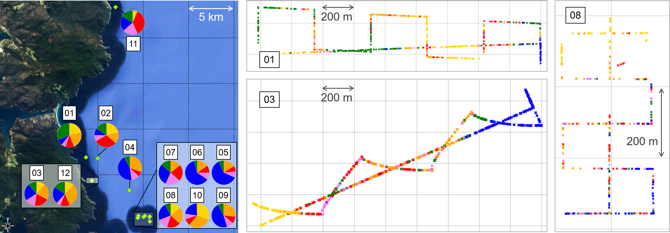
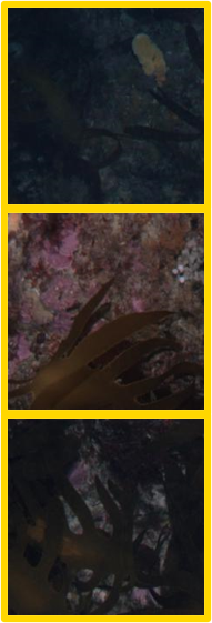
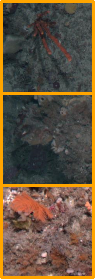
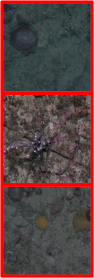
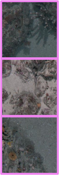
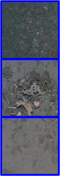
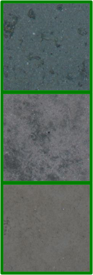
The Tasmania dataset used for evaluating the proposed GeoCLR [Williams et al., 2012] is shown in Figure 2 and described in Table 1. The dataset consists of 86,772 seafloor images taken by the Australian Centre for Field Robotics’ Sirius AUV from a target altitude of 2 m. The dataset contains habitat and substrate distributions as shown in Figure 3, including kelp (A), a registered essential ocean variable, and rocky reefs (B,C,D), which can form habitats for various conservation targets such as coral and sponges [Moltmann et al., 2019]. 5,369 randomly selected images are annotated by human experts into 6 classes, as shown in Figure 3. 50 images randomly selected from each 6 classes (total of 300 images) are used for validation and images selected from the remaining 5,069 annotated images are used for training, following the evaluation protocol described in subsection 4.3. The georeference information of each image is determined based on the stereo SLAM pipeline described in [Mahon et al., 2008, Johnson-Roberson et al., 2010]. The original resolution of the images is 1,360 1,024, where the average distance between adjacent images is approximately 0.5 m, so some images partly overlap each other. Prior to analysis, each image in the dataset is re-scaled to a resolution of 2 mm/pixel based on the imaging altitude. Randomly cropped 224 224 regions of the images are used for training, where validation is performed on the the same sized regions cropped from the centre of the images.
4.2 GeoCLR Training Configuration
GeoCLR can by used to train any type of CNN. Here we use the well established ResNet18 [He et al., 2016] for benchmarking. The latent representation and dimensions are set to and , respectively. A minibatch size of , learning rate of , weight decay of , temperature in equation(1) was used for all experiments. The threshold of closeness and depth scaling factor in equation 3 were set to and , respectively. The value for is conservative compared to the expected substrate and habitat patch size in the surveyed region, and was chosen to yield 2 to 4 nearby images based on the average distance between images (see Table 1). This minimises the probability of non-similar image pairs being selected near patch boundaries and the likelihood of duplicate pairs being selected during training. Results on the sensitivity of learning performance to a range of m included in the Appendix demonstrate this trend, with no benefit seen beyond m for the dataset analysed in this paper. As expected, a small value of is advantageous, with the limit of sufficiently nearby images being unavailable if it is set too small. The mean range between best and worst performing conditions is 3.7 % for equivalent and numbers. The value of was chosen to evenly treat horizontal and vertical displacement between images. Analysis in the Appendix for shows that the performance sensitivity small. The mean range between best and worst performing conditions is 1.7 % for equivalent and numbers. The sensitivity and optimum value for is likely to be dataset dependent, and more significant in datasets that have high rugosity.
Other than the method for generating similar image pairs, identical parameters were used for GeoCLR and SimCLR to allow for comparison. Both method are trained on the all 86,772 images in the dataset. We also benchmark the performance of the proposed method against conventional supervised transfer learning using ResNet18 that was pre-trained on ImageNet.
Though deeper CNN architectures, larger minibatch sizes and epoch are known to provide accuracy gains for SimCLR, these above parameters are set considering the computational power that can be reasonably deployed in the field, where access to high-performance computers networks is limited. The workstation used for experiments in this paper used a single NVIDIA TITAN RTX with 24 GB VRAM. The GeoCLR training and fine tuning with pseudo-labelling carried out in this work each took approximately a day (26 hours for GeoCLR training and a few minutes for fine-tuning) for the dataset of ~86k images gathered in 24 hours of bottom time over multiple AUV dives. This indicates that the results could be made available in timeframes relevant to assist planning and interpretation between dives during multi-day field expeditions.
4.3 Evaluation Protocol
CNNs trained using three different approaches (ImageNet, SimCLR, GeoCLR) are evaluated following the protocol used by [Chen et al., 2020]. Once the CNNs are trained, the latent representations they generated are analysed using different classifiers; a linear logistic regression, a non-linear Support Vector Machine with a Radial Basis Function kernel (SVM with RBF), and a fine-tuned CNN classifier. The logistic regression and SVM with RBF are both trained on the latent representation space output of ResNet18 after CNN training. For fine-tuning, a minibatch size of 256, Adam optimiser with learning rate of and no weight decay. The macro averaged f1 score over 6 classes determined from the independent validation set is used to compare the classification accuracy of each training method. All experiments are repeated ten times in each configuration, where the standard deviation (SD) of scores is shown alongside the mean value to describe variability.
We perform experiments to evaluate classification performance using training examples selected using the following sampling strategies:
-
•
Balanced: annotated images are selected so that all classes are equally represented.
-
•
Random: annotated images are randomly selected without any constraint.
-
•
H-means: annotated images are selected using hierarchical means to evenly represent different regions of the latent representation space learned through self-supervised training.
Class-balanced training examples can be considered ideal for supervised learning in applications where all classes are of equal importance. However, this requires significant human effort to determine the relevant classes and identify images corresponding to each class, which is not practical for most field survey scenarios. The random method is relevant for most survey scenarios, and can make the effort in annotation more manageable in situations where the class distribution in the target dataset is not known. However, the method suffers when the number of images in each class is not balanced, since classes are represented in proportion to their relative abundance, those with small populations tend to exhibit poor performance. The hierarchical means clustering [Nister and Stewenius, 2006], or H-means, method allows for balanced representation of the variety of images present in a dataset without the need for additional human effort, and was shown to be effective for guiding human labelling effort in [Yamada et al., 2022]. In this method, means clustering is first applied to latent representations with to find representative clusters of images in the dataset. An appropriate value for can be automatically determined for each dataset using the elbow method [Satopaa et al., 2011], where a value of was found to be appropriate for the dataset used in this experiment. Next, each cluster is further subdivided using means clustering where , to identify images closest to the centroid of each subdivided cluster, which is prioritised for human annotation. If the latent representations describe original images appropriately, the cluster boundaries found in the first means clustering are expected to approximate the class boundaries, allowing the class imbalance problem in random selection to be eased by selecting the same number of images from each cluster. The second means clustering avoids selecting similar samples from within each cluster, so that the full variety of images in the dataset can be represented by a small number of annotations. This H-means selection was shown to outperform random selection when appropriate latent representations are generated [Yamada et al., 2022]. The same work also demonstrated the use of pseudo-labels, generated from the predictions of classical classifiers applied to the latent representations, for CNN fine-tuning, which is also examined in this work.
Two sets of experiments are performed. First, we assess the performance of CNNs using the balanced selection strategy. Although this is not realistic for practical field scenarios, the results represent the expected upper bound of performances, and allows the fundamental performance of the three latent representation learning strategies (ImageNet, SimCLR, GeoCLR) to be compared. The second set of experiments compares the performance using random and H-means based selection strategies, including the use of pseudo labelling with linear logistic regression (PL-linear), a non-linear SVM with RBF (PL-SVM) for CNN fine-tuning. The sampling strategies can both realistically be implemented in field survey scenarios since they do not assume any prior knowledge of the datasets, and the images that require annotation can be rapidly identified in a fully unsupervised manner.
4.4 Result
4.4.1 Class-balanced training evaluation
| Config. Label | CNN Training | Classifier | Number of Annotations () | ||||
|---|---|---|---|---|---|---|---|
| 40 | 100 | 200 | 400 | 1000 | |||
| A1 | ImageNet | linear | 54.94.7 | 61.62.8 | 63.02.2 | 67.52.2 | 67.42.1 |
| A2 | ImageNet | SVM | 47.04.9 | 55.34.9 | 60.22.3 | 66.21.1 | 69.71.1 |
| A3 | ImageNet | Res18 | 58.92.6 | 65.52.7 | 68.22.5 | 71.21.7 | 73.81.3 |
| B1 | SimCLR | linear | 62.52.7 | 65.22.8 | 67.11.2 | 69.22.2 | 71.81.0 |
| B2 | SimCLR | SVM | 62.42.7 | 66.91.8 | 69.21.8 | 71.81.4 | 74.11.0 |
| B3 | SimCLR | Res18 | 53.44.4 | 61.32.2 | 65.52.0 | 68.92.7 | 72.40.9 |
| C1 | GeoCLR | linear | 63.82.9 | 67.82.4 | 71.41.4 | 72.91.8 | 74.91.0 |
| C2 | GeoCLR | SVM | 61.72.5 | 70.12.4 | 74.51.4 | 75.81.4 | 78.31.1 |
| C3 | GeoCLR | Res18 | 53.65.3 | 62.82.2 | 66.22.9 | 69.51.9 | 73.21.3 |
The CNNs are trained using three different method (Supervised Learning by ImageNet, SimCLR and GeoCLR). The latent representations () extracted from the annotated images by each CNN are used for logistic regression classification (linear) and SVM (with RBF) training. Also the CNNs are fine-tuned on the same subsets of images. The images are selected so that all 6 classes in the dataset are evenly described. The classifiers are trained 10 times with different random seed, and mean and SD values of f1 scores (macro averaged) are shown. The best score for each is shown as bold.
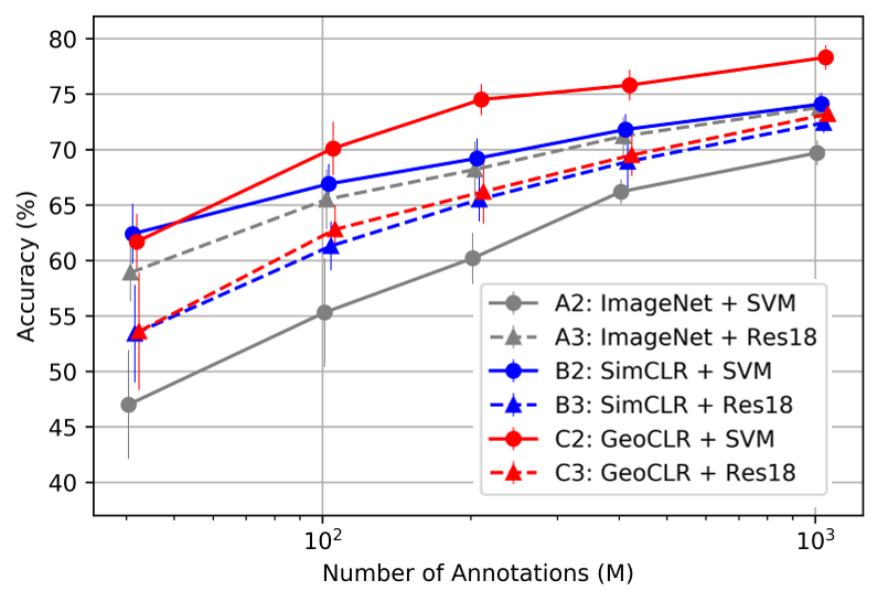
Table 2 shows the macro averaged f1 scores of each CNN training and classifier configuration on the class-balanced subsets of the annotated images. The results show that GeoCLR has the best performance for all values of , with the linear classifier (C1) showing the best performance for , and the SVM classifier (C2) best for all other values. The latent representations generated using GeoCLR achieves an average 7.4 % and 5.2 % increase in performance compared to the best performing ImageNet and SimCLR trained configurations.
Among the ImageNet pre-trained CNN (A), the CNN fine-tuned using images (A3) achieves the highest accuracy for all with an average performance gain of 6.6 %. This is owed to the capacity of CNNs to simultaneously optimise feature extraction and classification during training. In A1 and A2, the lower level feature extractor optimised on ImageNet is not updated. The inferior performance compared to A3 indicates that the latent representations generated using ImageNet are suboptimal for the seafloor images used in this work, failing to describe their useful distinguishing features.
In contrast, for SimCLR and GeoCLR trained CNNs (B and C) the fine-tuned scores for the ResNet18 classifier are lower than the scores of linear and SVM classifier. This shows that the constraining effect of contrastive learning in SimCLR or GeoCLR training generates highly optimised latent representations. Since conventional fine-tuning does not maintain this constraining effect, it degrades performance, achieving a similar level of accuracy as fine-tuning of ImageNet pre-trained CNN in A3 for larger values if . This finding is in contrast to the results of [Chen et al., 2020], where fine-tuning of CNNs trained using SimCLR significantly outperform linear classifiers applied to latent representation space for generic terrestrial image datasets analysed. Possible reasons for the difference in behaviour is the relatively high dimensionality of () compared to the small number of classes (6) in the dataset considered in this paper, combined with the continuous transition of image appearance across the class boundaries, both of which are different to terrestrial benchmark datasets, which typically have a larger number of classes with discrete boundaries, both of which can make the latent representation more sensitive to the constraining effect of contrastive learning.
Figure 5(a) shows representative configurations from Table 2. The proposed GeoCLR with a SVM classifier (C2) outperforms all other configurations except for B2 when . Having said this, the best performance for is achieved by the GeoCLR with a linear classifier (C1) as can be seen in Table 2. When the CNNs are fine-tuned, transfer learning with ImageNet (A3) outperforms fine-tuned SimCLR and GeoCLR (B3 and C3).
4.4.2 Data selection method comparison
| Config. Label | CNN Training | Classifier | Data Selection | Number of Annotations () | ||||
|---|---|---|---|---|---|---|---|---|
| 40 | 100 | 200 | 400 | 1000 | ||||
| D1 | ImageNet | linear | random | 45.45.8 | 57.03.2 | 61.32.8 | 63.32.9 | 67.52.2 |
| D2 | ImageNet | linear | H-means | 49.55.6 | 58.04.7 | 64.43.4 | 66.52.6 | 68.81.8 |
| D3 | ImageNet | SVM | random | 35.54.4 | 50.23.7 | 58.43.3 | 63.71.4 | 67.91.0 |
| D4 | ImageNet | SVM | H-means | 43.03.4 | 57.52.8 | 63.71.0 | 67.01.4 | 69.71.3 |
| D5 | ImageNet | Res18 | random | 55.53.1 | 63.23.2 | 67.02.0 | 69.72.4 | 72.82.3 |
| D6 | ImageNet | Res18 | H-means | 51.85.7 | 64.12.0 | 67.62.7 | 73.11.3 | 74.11.7 |
| D7 | ImageNet | Res18 | PL-linear | 51.95.7 | 62.24.5 | 68.61.8 | 70.92.0 | 71.92.3 |
| D8 | ImageNet | Res18 | PL-SVM | 46.45.4 | 58.93.4 | 67.11.6 | 69.91.7 | 72.62.1 |
| E1 | SimCLR | linear | random | 55.04.0 | 63.83.0 | 66.32.1 | 67.73.2 | 71.21.1 |
| E2 | SimCLR | linear | H-means | 61.92.6 | 66.51.6 | 68.21.4 | 69.32.7 | 69.51.9 |
| E3 | SimCLR | SVM | random | 47.25.5 | 64.52.4 | 68.81.6 | 72.02.2 | 73.50.7 |
| E4 | SimCLR | SVM | H-means | 58.02.0 | 67.61.5 | 70.91.3 | 71.71.8 | 73.71.5 |
| E5 | SimCLR | Res18 | random | 49.57.5 | 60.32.2 | 64.52.4 | 67.71.8 | 71.52.3 |
| E6 | SimCLR | Res18 | H-means | 56.43.3 | 65.22.2 | 66.21.7 | 69.32.0 | 70.11.2 |
| E7 | SimCLR | Res18 | PL-linear | 64.32.2 | 68.81.4 | 69.51.7 | 70.51.7 | 72.81.3 |
| E8 | SimCLR | Res18 | PL-SVM | 63.12.8 | 69.81.8 | 70.61.1 | 72.71.1 | 72.90.8 |
| F1 | GeoCLR | linear | random | 58.95.0 | 67.82.7 | 70.81.7 | 72.72.5 | 75.11.4 |
| F2 | GeoCLR | linear | H-means | 65.82.9 | 70.51.7 | 72.82.0 | 73.02.1 | 74.62.5 |
| F3 | GeoCLR | SVM | random | 53.25.9 | 68.83.1 | 72.92.2 | 75.51.0 | 77.51.2 |
| F4 | GeoCLR | SVM | H-means | 55.34.2 | 71.81.6 | 74.61.5 | 76.61.2 | 79.01.0 |
| F5 | GeoCLR | Res18 | random | 49.57.9 | 60.33.8 | 65.21.7 | 69.03.0 | 73.21.9 |
| F6 | GeoCLR | Res18 | H-means | 56.53.4 | 65.51.4 | 66.81.9 | 70.91.3 | 73.91.7 |
| F7 | GeoCLR | Res18 | PL-linear | 64.22.5 | 71.72.3 | 72.71.6 | 73.51.4 | 75.71.6 |
| F8 | GeoCLR | Res18 | PL-SVM | 63.72.1 | 72.02.1 | 72.51.5 | 74.31.0 | 75.21.3 |
The same CNNs as Table 2 where different data selection strategies (random and -means are used in the downstream classification task. In contrast to the balanced selection strategy shown in Table 2, these selection strategies do not require prior analysis by humans and so are available for analysis of data as it get collected in the field. The same classifiers (linear, SVM, fine-tuned ResNet18) are investigated. For fine-tuning the CNNs, pseudo-labels generated by linear classifier (-7) or SVM (-8) are used. The classifiers are trained 10 times with different random seed, and mean and SD values of f1 scores (macro averaged) are shown. The best score for each is shown as bold.
The performance using the random and H-means training data selection strategies, both of which do not need prior human input to understand the datasets, are shown in Table 3 for different values of .
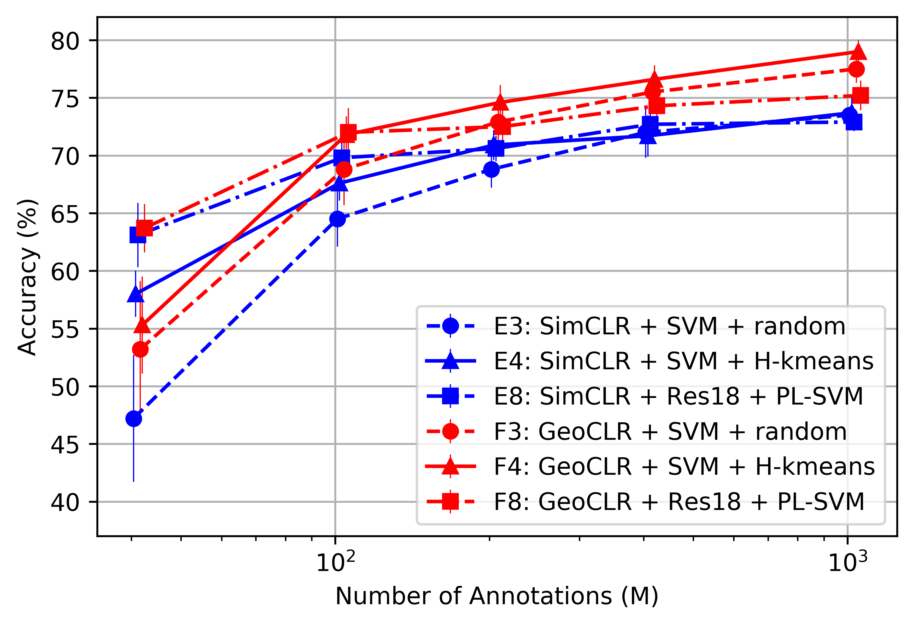
The different CNN training methods shows the same trend as the previous results with balanced training data selection (Table 2). When the classifiers are trained on the latent representations, GeoCLR outperforms SimCLR and ImageNet pre-training, achieving and average performance gains of 6.3 % and 20.0 %, respectively across all . As previously observed, fine-tuning SimCLR and GeoCLR trained CNNs degrades their performance. However, the pseudo-labelling introduced in (E7, E8, F7, F8) mitigates this effect by using a larger number of images for fine-tuning, which avoids the problem of overfitting that can occur when only a small number of images are used in fine tuning. This effect is strongest for small values of , where performance gains of 13.1 % and 8.0 % are achieved for both GeoCLR and SimCLR compared to equivalent configurations that do not use PL.
Figure 5(b) shows representative configurations in Table 3. The configurations with the GeoCLR (F) outperform their counterparts with the SimCLR (E) except for the case where where E4 performs better than F4. In general, the use of H-means improves performance compared to equivalent random configurations, achieving performance gains of 13.1 % and 5.7 % respectively for . Although the gain in performance reduces for larger , for GeoCLR H-means selection always improves performance compared to equivalent random configurations for all values of . An important observation is that the proposed GeoCLR achieved the best performance for all values of for both the balanced and H-means selection strategies.
A comparison between Table 2 and Table 3 shows that GeoCLR with H-means performs better than with the balanced selection strategy for all values of , with gains of 3.1 % and 2.7 % for small values of , and averaging a performance gain of 1.6 %.
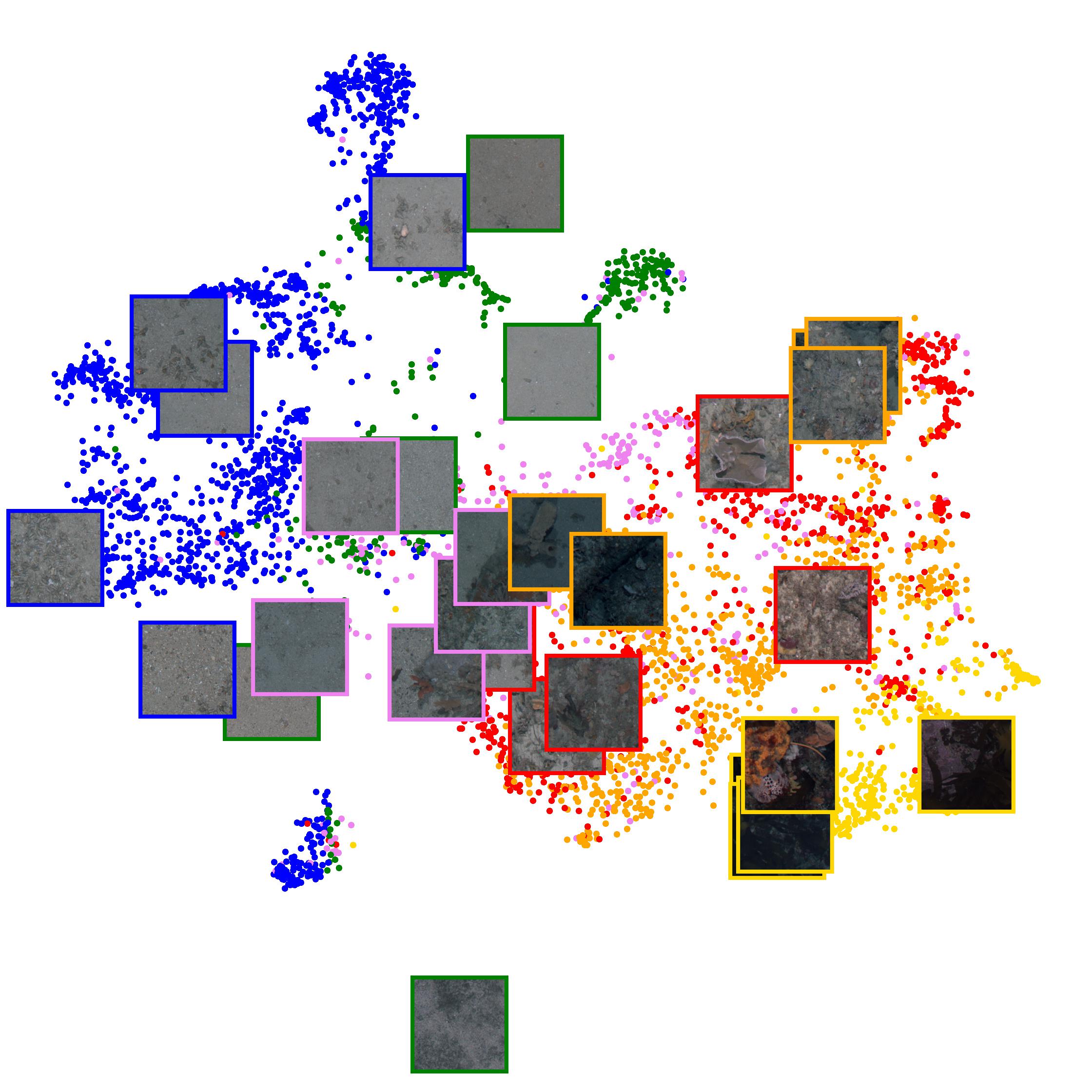
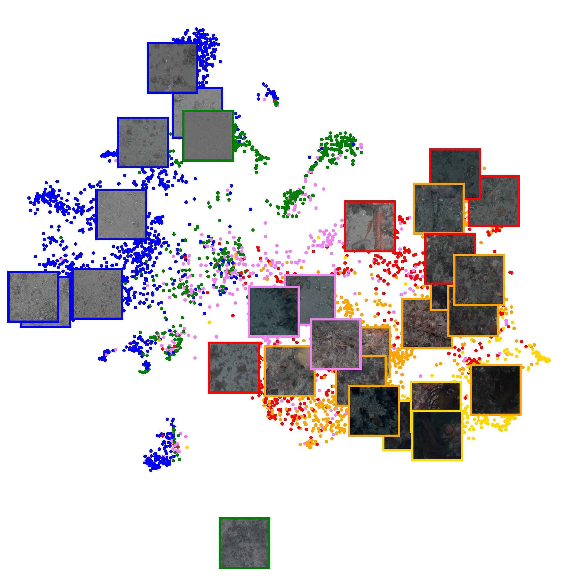
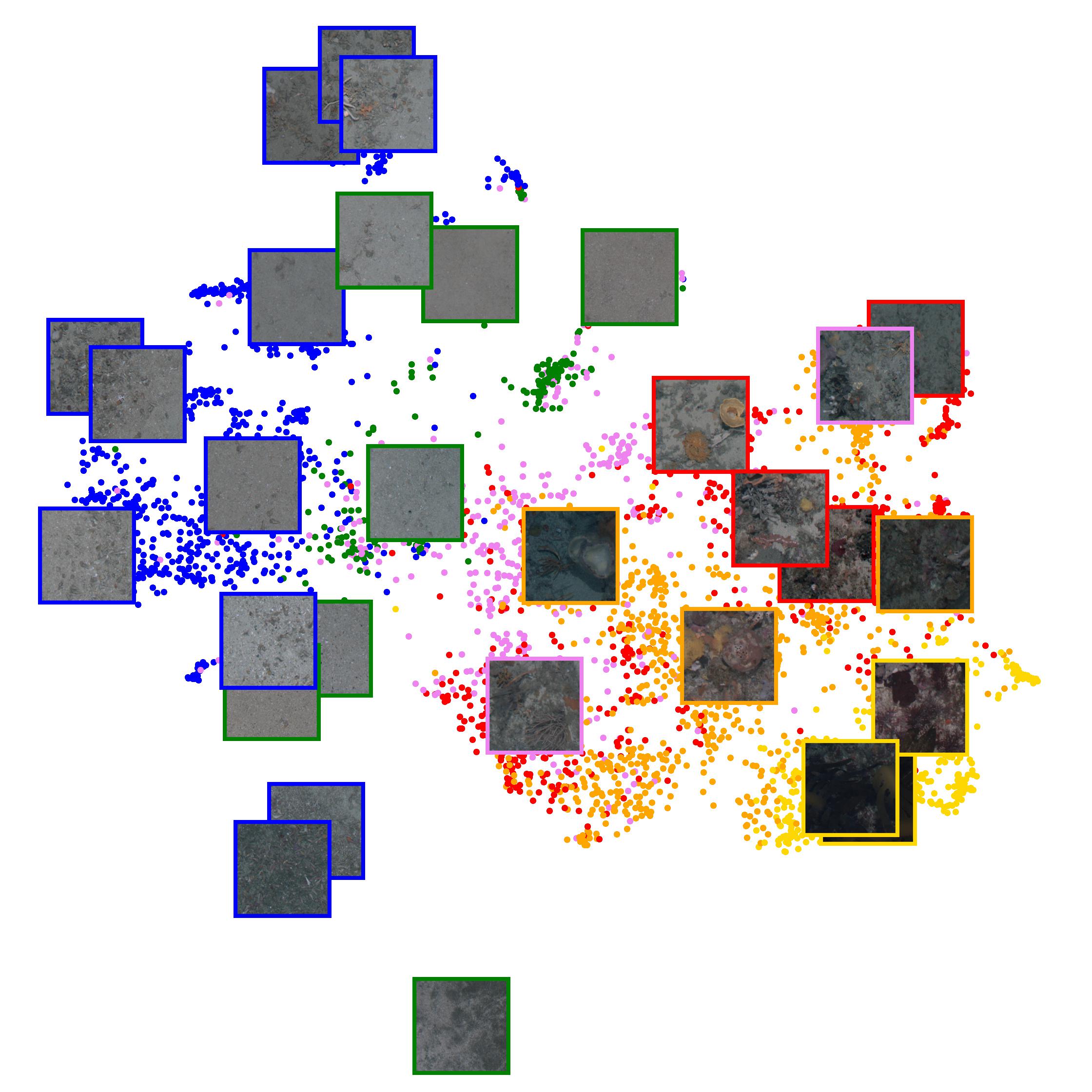
The results indicates that it is more valuable and informative to provide training data that evenly describes the latent representation space generated during self-supervised training, than it is to provide training data that evenly describes the targets that are of final interest to humans. Figure 4 shows the representative images selected by (a) Balanced, (b) Random and (c) H-kmeans strategies based on their location in the GeoCLR latent representations embedded by -SNE[Maaten and Hinton, 2008]. In this figure, images are shown for ease of visualisation, where the background points show the image representations that are not selected. The colour of the points and selected image borders illustrate the human class annotation of each annotated image using the same colour key as Figure 3. The visualisation shows that random selection strategy fails to select images from the central region of the latent representation space that is relatively sparsely populated. On the other hand, H-kmeans selects images evenly from the different regions of the latent representation. When compared to the balanced selection strategy, it can be seen that there are several regions of the latent representation space that are not sampled. This is because they are mapped to different regions of the latent space as more densely populated regions that have the same class. These undersampled regions of the latent space can be easily confused by a classifier, where the final assigned class will depend on the distribution of nearby training samples.
From a practical perspective, the proposed GeoCLR with H-means machine prioritised annotations and the SVM-RBF classifier (F4), and PL-SVM fine tuning (F7) achieves the same accuracy as state-of-the-art transfer learning (i.e. D5 ) using an order of magnitude fewer human annotations. The method also achieves the same accuracy as state-of-the-art contrastive learning approaches (i.e. E3 ) using a quarter of the annotations, where prior works rely on random data annotations and do not propose a data selection strategy. We consider being able to perform accurate classification with a relatively small number of labels (i.e. 0.1 % of the entire dataset) an important development since providing 100 annotations represents a level of human effort that can be justified for most application in the field. We also show that for applications that can justify a larger amount of human effort (i.e. ), the proposed GeoCLR outperforms conventional transfer learning (D5) and contrastive learning (E3) by 8.5 % and 7.5 % respectively. In addition to the demonstrated performance gains, the use of GeoCLR consistently improves performance over alternative configurations for all conditions tested in this work, and machine guided annotation H-means benefits performance for all configurations where , and although the performance gains diminish for larger , it never leads to significant performance reduction. The results indicate that these approaches can robustly improve the performance of CNNs for seafloor image interpretation.
4.5 Applications
Determining seafloor habitat class distributions is a fundamental task for marine monitoring and conservation. Here we apply the proposed GeoCLR method to estimate the relative proportion of habitat classes and map their physical distribution.
4.5.1 Estimating relative habitat class proportion
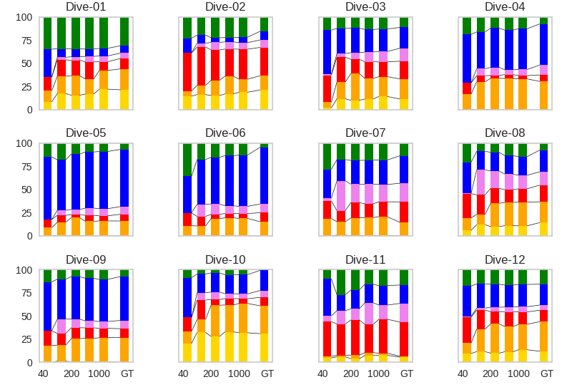
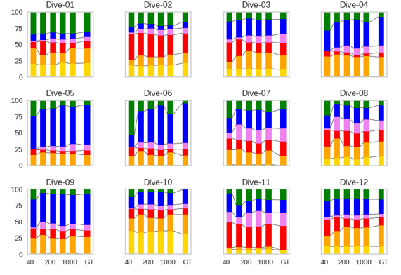
Figure 6 shows the relative proportion of different habitat classes estimated for machine prioritised annotations for each of the 12 dives in the Tasmania dataset. These are compared to the relative proportions for each dive where all human annotations have been used (i.e. average 450 annotations per dive) which we consider to be the ground truth here. The equivalent number of annotations per dive for the proposed method average approximately 3 annotations per dive for to approximately 83 per dive for . The results show that the estimated proportions approach the ground truth distributions for all dives, with the expected result that performance increases as a larger number of annotations are used for classifier training. The estimated proportions are poor for several of the dives with when using the F4 SVM classifier (Figure 6(a)), whereas the F8 fine-tuned with pseudo-labels generated by the SVM is generally more robust, approximating the ground truth class proportions better for the same number of training examples (Figure 6(b)). This indicates that the SVM classifier (F4) may be overfitting the latent representation space generated by GeoCLR when the number of annotations available is small, where this effect is mitigated by providing a larger number of training examples through pseudo-labels. However, there are some exception (Dives 06 and 07) to this and so the outputs with should be treated with caution where validation data is not available. On the other hand, for both methods (i.e. F4 and F8) perform robustly for all dives, with F4 outperforming F8 and providing more stable estimates for different values of . This is due to the fact that the latent representation space remains the same regardless of as no CNN re-training takes place.
4.5.2 Habitat mapping
The physical distribution of habitats is important for conservation since it influences the distribution of organisms near the seafloor. It is also important for understanding ecosystem health as benthic habitats such as kelp (seen here) and coral are classified as essential ocean variables.
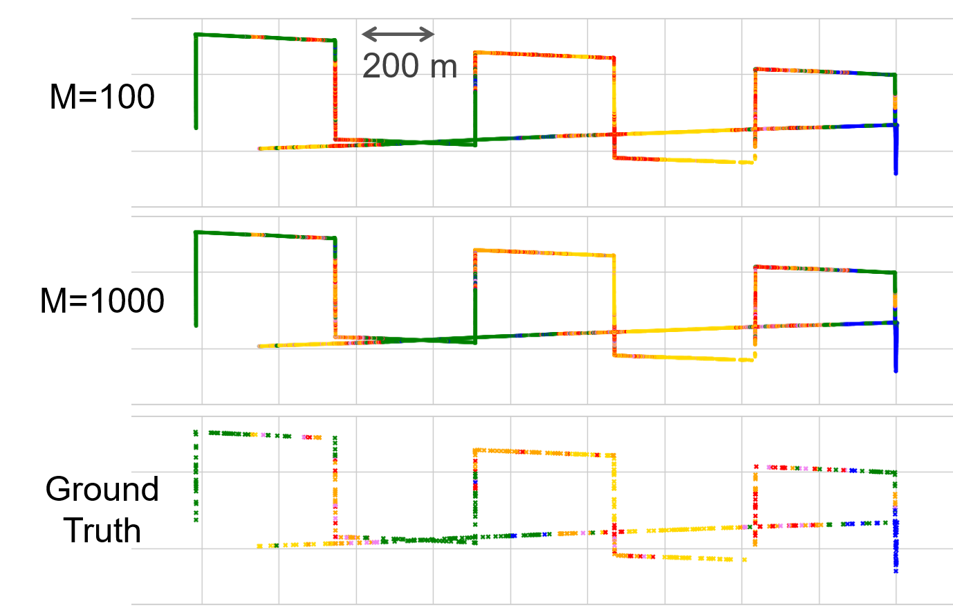
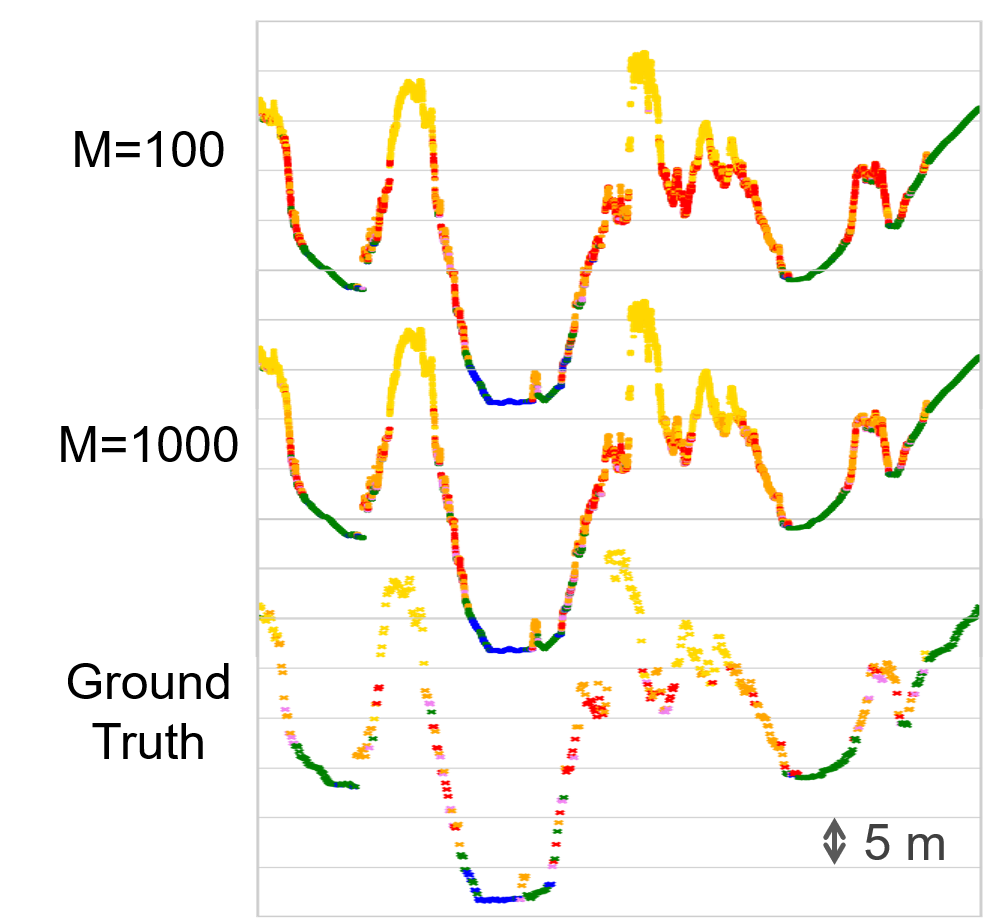
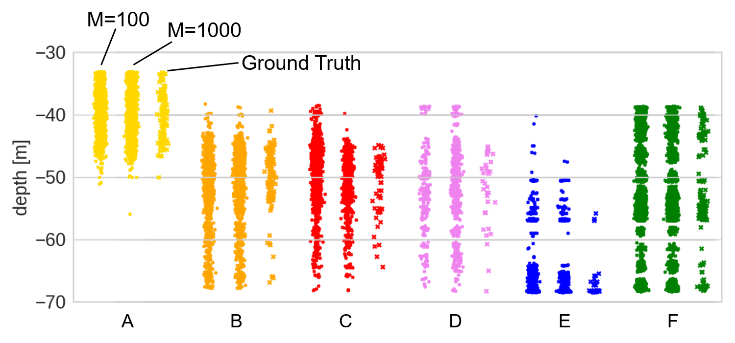
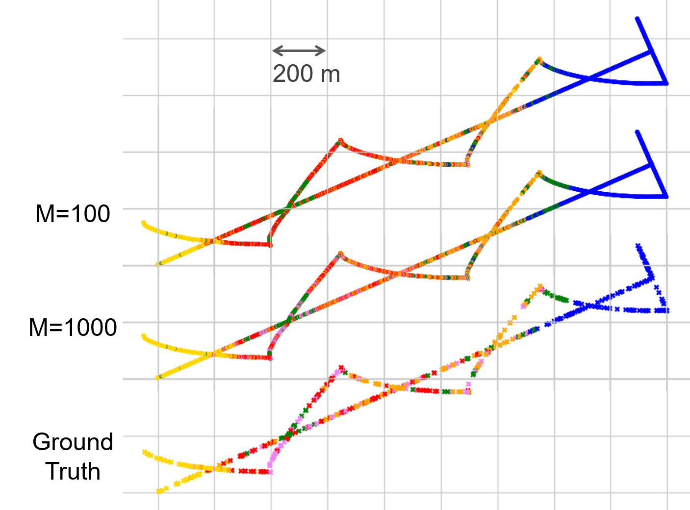
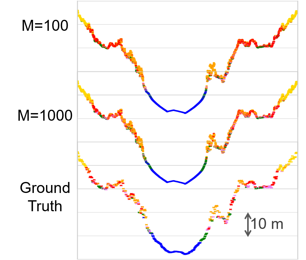
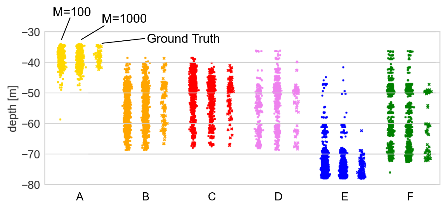
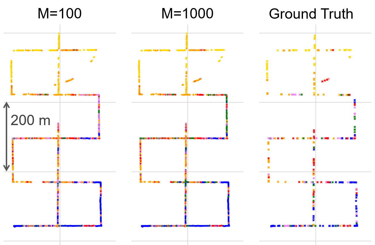
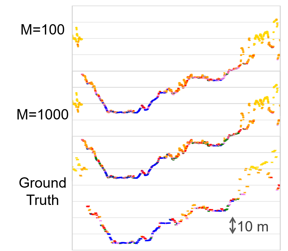
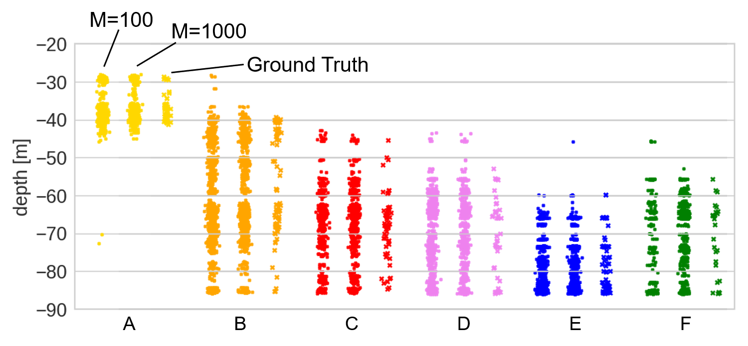
The proposed method allows efficient estimation of habitat maps based on the 3D location where each classified image was taken. Here, we show the horizontal distributions of the classes, the depth profiles vs. image index, and the class vs. depth distributions are shown in Figures 7, 8 and 9 for three dives (01,03 and 08) which were chosen as representative cases. The figures show habitat maps generated using GeoCLR for {,F8}, {,F4} in Table 3 and the ground truth labels.
The results show that both {,F8} and {,F4} configurations closely approximate the ground truth horizontal and vertical habitat class distributions, capturing the continuous spatial transitions between Kelp (A), Low Relief Reef (C), High Relief Reef (B) to Screw Shell Rubble (E) or Sand (F). The class vs depth distributions show that the larger values of provide a better approximation of vertical class distribution, which is an expected result. However, for classes that exist in a limited depth band (e.g. Kelp (A), Screw Shell Rubble (E)) both values of capture this trend.
5 Conclusion
The paper has developed a method to leverage georeferenced information in contrastive learning for efficient training of deep-learning CNNs. The proposed Georeference Contrastive Learning for seafloor image Representation (GeoCLR) method is effective for datasets where the targets of interest for semantic interpretation are distributed over spatial scales larger that the footprint of a single image frame. The underlying assumption is that images gathered within a close distance are more likely to have similar visual appearance than images that are taken far apart. This assumption can be reasonably satisfied in seafloor robotic imaging applications, where 1) images are acquired at close and regular intervals along a vehicle’s trajectory, and 2) the targets for interpretation are substrates and habitats which typically have extents much greater than the image footprint. The method can be deployed on any CNN, and performance gains can be achieved without any prior human input to interpret the dataset. We demonstrate the performance of the proposed training method using a CNN architecture that can be deployed on computers that can be reasonably expected to be available during a field survey, without relying on network access to supercomputers, and can generate results in timeframes that are relevant for on-going field expeditions. Experiments on a robotically obtained seafloor image dataset that includes more than ~86k images and ~5k annotations show that:
-
•
The proposed GeoCLR method outperforms existing state-of-the-art contrastive learning (SimCLR) and transfer learning for downstream supervised classification tasks using an equivalent CNN architecture (ResNet18). On an ideal, class balanced training dataset, the SVM with RBF kernel trained on the features extracted by the GeoCLR trained CNN shows an average of 5.2 % and maximum of 7.7 % improvement compared to the accuracy scores of SimCLR for annotations. Compared to ResNet18 trained by transfer learning, an average improvement of 7.4 %, a maximum of 9.2 % is achieved.
-
•
The representations extracted by the GeoCLR are useful for identifying representative images for prioritised human annotation in a fully unsupervised manner. This can improve the performance and efficiency of human effort for classification, where selecting a prioritised training dataset using H- means clustering increases the classification accuracy by an average of 4.9 % and maximum of 14.1 % compared to random selection, where the performance gains are more significant for small numbers of . Compared with SimCLR, GeoCLR latent representations shows 7.1 % better score on average with randomly annotated training datasets. Prioritised annotating by H-means allows score improvements for all values, leading to 10.2 % increase in total.
-
•
Selecting representative images for prioritised labelling based on their distribution in the GeoCLR latent representation space results in better performance than providing class-balanced annotated examples. The machine driven H-means selection strategy achieves an average of 1.6 % and maximum of 3.1 % increase in accuracy compared to the class-balanced selection strategy for an equivalent number of annotations, where greater gains are achieved for small numbers of annotations. This indicates that it is more informative to provide training data that evenly describes the latent representation space generated during self-supervised training, than it is to provide training data that evenly describes the targets that are of final interest to humans.
-
•
The combination of GeoCLR and H-means achieves the same accuracy as state-of-the-art transfer learning using an order of magnitude fewer human annotations, and state-of-the-art contrastive learning approaches using a quarter of the labels. This allows the proportion of habitat classes and their spatial distribution to be accurately estimated () annotating only 0.1 % of the images in the dataset. This is significant as providing approximately 100 annotations represents a level of human effort that can be justified for most field application. For applications where a greater level of human effort is available, we show that with 1000 annotations, the proposed GeoCLR outperforms conventional transfer learning and contrastive learning by 8.5 % and 7.5 % respectively, achieving a classification accuracy of . The combination of GeoCLR and H-means never degraded performance compared to equivalent alternative configurations in the experiments described in this paper.
Acknowledgements
This work was carried out under the UK Natural Environment Research Council’s Oceanids Biocam project NE/P020887/1 and Australian Research Council’s Automated Benthic Understanding DP190103914 Discovery project.
References
- Beijbom et al., 2012 Beijbom, O., Edmunds, P. J., Kline, D. I., Mitchell, B. G., and Kriegman, D. (2012). Automated annotation of coral reef survey images. In 2012 IEEE Conference on Computer Vision and Pattern Recognition, pages 1170–1177. IEEE.
- Bewley et al., 2015 Bewley, M., Nourani-Vatani, N., Rao, D., Douillard, B., Pizarro, O., and Williams, S. B. (2015). Hierarchical classification in AUV imagery. In Field and service robotics, pages 3–16. Springer.
- Chen et al., 2020 Chen, T., Kornblith, S., Norouzi, M., and Hinton, G. (2020). A simple framework for contrastive learning of visual representations. In International conference on machine learning, pages 1597–1607. PMLR.
- Deng et al., 2009 Deng, J., Dong, W., Socher, R., Li, L.-J., Li, K., and Fei-Fei, L. (2009). Imagenet: A large-scale hierarchical image database. In 2009 IEEE conference on computer vision and pattern recognition, pages 248–255. Ieee.
- Goyal et al., 2017 Goyal, P., Dollár, P., Girshick, R., Noordhuis, P., Wesolowski, L., Kyrola, A., Tulloch, A., Jia, Y., and He, K. (2017). Accurate, large minibatch sgd: Training imagenet in 1 hour. arXiv preprint arXiv:1706.02677.
- He et al., 2016 He, K., Zhang, X., Ren, S., and Sun, J. (2016). Deep residual learning for image recognition. In Proceedings of the IEEE conference on computer vision and pattern recognition, pages 770–778.
- Jing and Tian, 2020 Jing, L. and Tian, Y. (2020). Self-supervised visual feature learning with deep neural networks: A survey. IEEE Transactions on Pattern Analysis and Machine Intelligence.
- Johnson-Roberson et al., 2010 Johnson-Roberson, M., Pizarro, O., Williams, S. B., and Mahon, I. (2010). Generation and visualization of large-scale three-dimensional reconstructions from underwater robotic surveys. Journal of Field Robotics, 27(1):21–51.
- Kaeli and Singh, 2015 Kaeli, J. W. and Singh, H. (2015). Online data summaries for semantic mapping and anomaly detection with autonomous underwater vehicles. In OCEANS 2015-Genova, pages 1–7. IEEE.
- Krizhevsky et al., 2012 Krizhevsky, A., Sutskever, I., and Hinton, G. E. (2012). Imagenet classification with deep convolutional neural networks. In Advances in neural information processing systems, pages 1097–1105.
- Le-Khac et al., 2020 Le-Khac, P. H., Healy, G., and Smeaton, A. F. (2020). Contrastive representation learning: A framework and review. IEEE Access.
- Maaten and Hinton, 2008 Maaten, L. v. d. and Hinton, G. (2008). Visualizing data using t-sne. Journal of machine learning research, 9(Nov):2579–2605.
- Mahmood et al., 2018 Mahmood, A., Bennamoun, M., An, S., Sohel, F. A., Boussaid, F., Hovey, R., Kendrick, G. A., and Fisher, R. B. (2018). Deep image representations for coral image classification. IEEE Journal of Oceanic Engineering, 44(1):121–131.
- Mahon et al., 2008 Mahon, I., Williams, S. B., Pizarro, O., and Johnson-Roberson, M. (2008). Efficient view-based SLAM using visual loop closures. IEEE Transactions on Robotics, 24(5):1002–1014.
- Moltmann et al., 2019 Moltmann, T., Turton, J., Zhang, H.-M., Nolan, G., Gouldman, C., Griesbauer, L., Willis, Z., Piniella, A. M., Barrell, S., Andersson, E., Gallage, C., Charpentier, E., Belbeoch, M., Poli, P., Rea, A., Burger, E. F., Legler, D. M., Lumpkin, R., Meinig, C., O’Brien, K., Saha, K., Sutton, A., Zhang, D., and Zhang, Y. (2019). A global ocean observing system (goos), delivered through enhanced collaboration across regions, communities, and new technologies. Frontiers in Marine Science, 6:291.
- Neettiyath et al., 2020 Neettiyath, U., Thornton, B., Sangekar, M., Nishida, Y., Ishii, K., Bodenmann, A., Sato, T., Ura, T., and Asada, A. (2020). Deep-sea robotic survey and data processing methods for regional-scale estimation of manganese crust distribution. IEEE Journal of Oceanic Engineering, pages 1–13.
- Nister and Stewenius, 2006 Nister, D. and Stewenius, H. (2006). Scalable recognition with a vocabulary tree. In 2006 IEEE Computer Society Conference on Computer Vision and Pattern Recognition (CVPR’06), volume 2, pages 2161–2168. Ieee.
- Ojala et al., 2002 Ojala, T., Pietikäinen, M., and Mäenpää, T. (2002). Multiresolution gray-scale and rotation invariant texture classification with local binary patterns. IEEE Transactions on Pattern Analysis & Machine Intelligence, (7):971–987.
- Oord et al., 2018 Oord, A. v. d., Li, Y., and Vinyals, O. (2018). Representation learning with contrastive predictive coding. arXiv preprint arXiv:1807.03748.
- Rao et al., 2017 Rao, D., De Deuge, M., Nourani-Vatani, N., Williams, S. B., and Pizarro, O. (2017). Multimodal learning and inference from visual and remotely sensed data. The International Journal of Robotics Research, 36(1):24–43.
- Satopaa et al., 2011 Satopaa, V., Albrecht, J., Irwin, D., and Raghavan, B. (2011). Finding a” kneedle” in a haystack: Detecting knee points in system behavior. In 2011 31st international conference on distributed computing systems workshops, pages 166–171. IEEE.
- Sohn, 2016 Sohn, K. (2016). Improved deep metric learning with multi-class n-pair loss objective. In Proceedings of the 30th International Conference on Neural Information Processing Systems, pages 1857–1865.
- Steinberg et al., 2011 Steinberg, D., Friedman, A., Pizarro, O., and Williams, S. B. (2011). A bayesian nonparametric approach to clustering data from underwater robotic surveys. In International Symposium on Robotics Research, volume 28, pages 1–16.
- Tan et al., 2018 Tan, C., Sun, F., Kong, T., Zhang, W., Yang, C., and Liu, C. (2018). A survey on deep transfer learning. In International conference on artificial neural networks, pages 270–279. Springer.
- Williams et al., 2012 Williams, S. B., Pizarro, O. R., Jakuba, M. V., Johnson, C. R., Barrett, N. S., Babcock, R. C., Kendrick, G. A., Steinberg, P. D., Heyward, A. J., Doherty, P. J., Mahon, I., Johnson-Roberson, M., Steinberg, D., and Friedman, A. (2012). Monitoring of benthic reference sites: Using an autonomous underwater vehicle. IEEE Robotics Automation Magazine, 19(1):73–84.
- Wu et al., 2018 Wu, Z., Xiong, Y., Yu, S. X., and Lin, D. (2018). Unsupervised feature learning via non-parametric instance discrimination. In Proceedings of the IEEE Conference on Computer Vision and Pattern Recognition, pages 3733–3742.
- Yamada et al., 2022 Yamada, T., Massot-Campos, M., Prugel-Bennett, A., Pizarro, O., Williams, S., and Thornton, B. (2022). Guiding labelling effort for efficient learning with georeferenced images. IEEE Transactions on Pattern Analysis and Machine Intelligence, Early Access.
- Yamada et al., 2021a Yamada, T., Massot-Campos, M., Prügel-Bennett, A., Williams, S. B., Pizarro, O., and Thornton, B. (2021a). Leveraging metadata in representation learning with georeferenced seafloor imagery. IEEE Robotics and Automation Letters, 6(4):7815–7822.
- Yamada et al., 2021b Yamada, T., Prügel-Bennett, A., and Thornton, B. (2021b). Learning features from georeferenced seafloor imagery with location guided autoencoders. Journal of Field Robotics, 38(1):52–67.
- Yang et al., 2009 Yang, J., Yu, K., Gong, Y., and Huang, T. (2009). Linear spatial pyramid matching using sparse coding for image classification. In 2009 IEEE Conference on computer vision and pattern recognition, pages 1794–1801. IEEE.
Appendix A Sensitivity to hyperparameters
The main contribution of the GeoCLR method is that selecting similar image pairs that are physically close to each other will provide a better representation of variability in contrastive learning than traditional data augmentation.
The conditions for a pair of images to be physically close enough is determined by the following equation (eq. (3) in the main text):
| (3) |
where is the 3D georeference of image . Eq. (3) includes two hyperparameters: , which corresponds to a 3D distance threshold where images captured within this range are regarded as similar, and , which is a weight for the depth difference between images. These hyperparameters relate to the physical characteristics of observed seafloor habitats and substrates, and so their optimised values are considered to be dataset dependent. This appendix investigates the sensitivity of learning performance to these hyperparameters for the Tasmania dataset considered in this work.
| Number of Annotations () | |||||
|---|---|---|---|---|---|
| 40 | 100 | 200 | 400 | 1000 | |
| 0.0 (SimCLR) | 62.52.7 | 65.22.8 | 67.11.2 | 69.22.2 | 71.81.0 |
| 1.0 | 63.82.9 | 67.82.4 | 71.41.4 | 72.91.8 | 74.91.0 |
| 3.0 | 59.72.7 | 64.42.4 | 69.23.4 | 70.82.1 | 72.81.4 |
| 5.0 | 61.12.2 | 65.92.4 | 68.41.6 | 71.11.8 | 71.92.3 |
| 10.0 | 60.52.5 | 66.13.0 | 68.52.5 | 70.53.1 | 72.91.7 |
is equivalent to SimCLR (B1 in Table 2).
Table A1 shows the f1 scores of linear classifiers trained on the obtained latent representations for different values ( m) for fixed . Class balanced training datasets with different numbers of images () have been used to train the classifier, which is the same configuration as B1 (for m) or C1 (others) in Table 2 of the main paper. The best performance is using m for all , showing that it is optimal for this dataset. Since the AUV travelled at with image acquisition at 1 fps, m is the smallest value where most images will have at least two nearby images to form a similar pair for contrastive learning. Larger values will have more images to chose from for the similar pair, but as the distances between the pair increases, we expect their appearances to become less similar. If is too small, there will be no nearby images to select from, and so only augmentation on the same image can be performed (i.e., the same as SimCLR). The latent representations obtained with the larger values ( m) show poorer performance scores than m for all . However, they still perform better than the original SimCLR ( m) except for a few cases with . It can be assumed that the optimal value depends on the habitat and substrate patch sizes in the observed area. Even if the size of these semantic patches is not known, we can expect smaller values to perform robustly since similar appearance image pairs are likely to be sampled, compared with larger , under the assumption that semantic patches of interest for habitat and substrate mapping occur on spatial scales larger than the footprint of a single image frame.
| Number of Annotations () | |||||
|---|---|---|---|---|---|
| 40 | 100 | 200 | 400 | 1000 | |
| 0.0 | 63.83.3 | 69.22.9 | 72.51.7 | 74.01.9 | 75.61.3 |
| 0.5 | 63.74.7 | 68.43.1 | 71.82.0 | 74.01.9 | 76.62.1 |
| 1.0 | 63.82.9 | 67.82.4 | 71.41.4 | 72.91.8 | 74.91.0 |
| 3.0 | 65.34.6 | 70.22.9 | 72.72.9 | 74.41.7 | 75.91.3 |
| 5.0 | 63.82.6 | 69.63.4 | 72.32.3 | 74.21.7 | 75.31.7 |
| 10.0 | 64.03.7 | 68.73.3 | 72.92.0 | 74.32.5 | 76.01.6 |
Table A2 shows the f1 scores trained latent representations obtained using the optimal value ( m) with the different values () for the Tasmania dataset. Increasing increases sensitivity to depth differences, making it more likely for a potential similar pair to be rejected if there is a difference in their depths. Though the scores differ slightly depending on the values, their standard deviation values show these differences within the margin of error. The reason why is less sensitive to the performance than can be considered that rugosity and slope in the Tasmania dataset are relatively small. For the datasets with more drastic depth changes we expect greater sensitivity to values.