Identification in Bayesian Estimation of the Skewness Matrix in a Multivariate Skew-Elliptical Distributionthanks: This research is supported by the Keio University Doctorate Student Grant-in-Aid Program from Ushioda Memorial Fund; and JSPS KAKENHI under Grant [number MKK337J].

Sakae Oya111sakae.prosperity21@keio.jp
Graduate School of Economics, Keio University, Tokyo, Japan
and
Teruo Nakatsuma
Faculty of Economics, Keio University, Tokyo, Japan
Abstract

Harvey et al. (2010) extended the Bayesian estimation method by Sahu et al. (2003) to a multivariate skew-elliptical distribution with a general skewness matrix, and applied it to Bayesian portfolio optimization with higher moments. Although their method is epochal in the sense that it can handle the skewness dependency among asset returns and incorporate higher moments into portfolio optimization, it cannot identify all elements in the skewness matrix due to label switching in the Gibbs sampler. To deal with this identification issue, we propose to modify their sampling algorithm by imposing a positive lower-triangular constraint on the skewness matrix of the multivariate skew-elliptical distribution and improved interpretability. Furthermore, we propose a Bayesian sparse estimation of the skewness matrix with the horseshoe prior to further improve the accuracy. In the simulation study, we demonstrate that the proposed method with the identification constraint can successfully estimate the true structure of the skewness dependency while the existing method suffers from the identification issue.


Keywords: Bayesian Estimation, Identification, Label Switching, Skew-Elliptical Distribution, Skewness Matrix.

1 Introduction

The mean-variance approach proposed by Markowitz (1952) still plays the central role in portfolio management even today. One of the key assumptions of this approach is that asset returns jointly follow a multivariate normal distribution, though it is well-known that they tend to follow a fat-tailed, possibly skewed distribution as Kon (1984), Mills (1995), Markowitz and Usmen (1996), Peiró (1999) among others have pointed out. Therefore, researches have proposed numerous distributions that can express these characteristics of asset returns well. In particular, a so-called skew-t distribution is often assumed for asset returns since Hansen (1994) first used it for modeling financial data. There are various types of skew-t distribution known in the literature, but arguably the most famous one is based on the generalized hyperbolic (GH) distribution.

The GH distribution, which was originally introduced by Barndorff-Nielsen (1977), can flexibly describe many distributions including the normal distribution, hyperbolic distribution, normal inverse Gaussian (NIG) distribution, Student’s t distribution, and skew-t distribution. The skew-t distribution as a special case of the GH distribution is called the GH skew-t distribution. Hansen (1994), Fernández and Steel (1998) and Aas and Haff (2006) assumed the GH skew-t distribution for asset returns. Especially, application of the GH distribution has been recently advanced in the field of asset price volatility models. For example, Nakajima and Omori (2012) assumed the GH skew-t distribution for the error distribution of the stochastic volatility (SV) model and proposed a Bayesian Markov chain Monte Carlo (MCMC) method while Nakajima (2017) constructed a sparse estimation method for the skewness parameter of the GH skew-t distribution in the SV model and demonstrated that it could improve prediction accuracy.

Although the GH distribution is flexible enough to model a single asset on many occasions, it has difficulty in capturing the skewness dependency among multiple assets. Fund managers would find the skewness dependency useful in particular when the financial market crashes and almost all assets suddenly go south since such sharp price co-movement may not be captured by the second moment (i.e., correlation) only.

To circumvent this shortcoming of the GH distribution, we propose to use the skew-elliptical distribution, which was proposed by Branco and Dey (2001) as a generalization of the multivariate skew-normal distribution by Azzalini and Valle (1996) and later improved by Sahu et al. (2003)222Although we take up the skew-elliptical distribution based on Sahu et al. (2003) with application to portfolio management in mind, there are alternative skew-elliptical-type distributions known in the literature. Research on skew-elliptical-type distributions to financial data is very active (e.g., Barbi and Romagnoli (2018), Carmichael and Coën (2013), Alodat and Al-Rawwash (2014)). Adcock and Azzalini (2020) reviews the recent development in this field and explains relationship among various types of skew-elliptical distribution in detail.. The skew-elliptical distribution includes the normal distribution, Student’s t distribution and their skewed counterparts: skew-normal and skew-t distribution. Unlike the GH distribution, it is straightforward to extend the skew-elliptical distribution to the multivariate case. The multivariate skew-normal distribution has another advantage: Its Bayesian estimation can be conducted via pure Gibbs sampling. For example, Sahu et al. (2003) proposed a Gibbs sampler for a linear regression model in which the error term follows a skew-elliptical distribution without skewness dependency. Moreover, Harvey et al. (2010) improved Sahu et al. (2003)’s method, and applied it to Bayesian estimation of the multivariate skew-normal distribution as well as portfolio optimization that considers up to the third moment in the presence of skewness dependency.

In our assessment, however, the Bayesian estimation method of the multivariate skew-elliptical distribution by Harvey et al. (2010) has an identification issue about the skewness parameters due to so-called label switching. To elaborate on our point, let us look into the definition of a multivariate skew-elliptical distribution. For simplicity, we only consider the multivariate skew-normal distribution333In essence, any skew-elliptical distributions have the same identification issue. So we start with the skew-normal distribution as a representative example. It is straightforward to extend our argument to any skew-elliptical distributions including the skew-t distribution which we will deal with in Section 3.. Suppose a N×1𝑁1N\times 1 random vector Rtsubscript𝑅𝑡R_{t} (t=1,,T)𝑡1𝑇(t=1,\dots,T) of asset returns follows a multivariate skew-normal distribution such that

Rtsubscript𝑅𝑡\displaystyle R_{t} =μ+ΔZt+ϵt,absent𝜇Δsubscript𝑍𝑡subscriptitalic-ϵ𝑡\displaystyle=\mu+\Delta Z_{t}+\epsilon_{t}, (1)
Ztsubscript𝑍𝑡\displaystyle Z_{t} 𝒩+(0,IN),ϵt𝒩(0,Ω1),formulae-sequencesimilar-toabsentsuperscript𝒩0subscript𝐼𝑁similar-tosubscriptitalic-ϵ𝑡𝒩0superscriptΩ1\displaystyle\sim\mathcal{N}^{+}(0,I_{N}),\quad\epsilon_{t}\sim\mathcal{N}(0,\Omega^{-1}),
Ztsubscript𝑍𝑡\displaystyle Z_{t} ϵt,perpendicular-toabsentsubscriptitalic-ϵ𝑡\displaystyle\perp\epsilon_{t},

where each element in Ztsubscript𝑍𝑡Z_{t} is supposed to independently follow a positive half normal distribution with the scale parameter equal to 1. ΔΔ\Delta and ΩΩ\Omega are the skewness matrix444Here we call ΔΔ\Delta the skewness matrix though it does not match the skewness of the distribution in this model. For more information, see Section 2.2 and Appendix A of Harvey et al. (2010). and the precision matrix555Harvey et al. (2010) used the covariance matrix in their specification of the skew-normal distribution and assumed the inverse-Wishart prior for it, which is equivalent to assuming the Wishart prior for the precision matrix in our specification. We use the precision matrix because we later examine the extended model that incorporates sparsity into the graphical structure among asset returns. respectively. Harvey et al. (2010) did not impose any restriction and assumed ΔΔ\Delta is full matrix :

Δ=[δ11δ12δ13δ1Nδ21δ22δ23δ2Nδ31δ32δ33δ3NδN1δN2δN3δNN].Δmatrixsubscript𝛿11subscript𝛿12subscript𝛿13subscript𝛿1𝑁subscript𝛿21subscript𝛿22subscript𝛿23subscript𝛿2𝑁subscript𝛿31subscript𝛿32subscript𝛿33subscript𝛿3𝑁missing-subexpressionsubscript𝛿𝑁1subscript𝛿𝑁2subscript𝛿𝑁3subscript𝛿𝑁𝑁\Delta=\begin{bmatrix}\delta_{11}&\delta_{12}&\delta_{13}&\cdots&\delta_{1N}\\ \delta_{21}&\delta_{22}&\delta_{23}&\cdots&\delta_{2N}\\ \delta_{31}&\delta_{32}&\delta_{33}&\cdots&\delta_{3N}\\ \vdots&\vdots&\vdots&&\vdots\\ \delta_{N1}&\delta_{N2}&\delta_{N3}&\cdots&\delta_{NN}\\ \end{bmatrix}.

By defining

R=[R1RT],R~=[R~1R~T]=[(R1μ)(RTμ)],Z=[Z1ZT],E=[ϵ1ϵT],formulae-sequenceformulae-sequence𝑅matrixsuperscriptsubscript𝑅1superscriptsubscript𝑅𝑇~𝑅matrixsuperscriptsubscript~𝑅1superscriptsubscript~𝑅𝑇matrixsuperscriptsubscript𝑅1𝜇superscriptsubscript𝑅𝑇𝜇formulae-sequence𝑍matrixsuperscriptsubscript𝑍1superscriptsubscript𝑍𝑇𝐸matrixsuperscriptsubscriptitalic-ϵ1superscriptsubscriptitalic-ϵ𝑇R=\begin{bmatrix}R_{1}^{\intercal}\\ \vdots\\ R_{T}^{\intercal}\end{bmatrix},\quad\tilde{R}=\begin{bmatrix}\tilde{R}_{1}^{\intercal}\\ \vdots\\ \tilde{R}_{T}^{\intercal}\end{bmatrix}=\begin{bmatrix}(R_{1}-\mu)^{\intercal}\\ \vdots\\ (R_{T}-\mu)^{\intercal}\end{bmatrix},\quad Z=\begin{bmatrix}Z_{1}^{\intercal}\\ \vdots\\ Z_{T}^{\intercal}\end{bmatrix},\quad E=\begin{bmatrix}\epsilon_{1}^{\intercal}\\ \vdots\\ \epsilon_{T}^{\intercal}\end{bmatrix},

(1) can be rewritten as

R~~𝑅\displaystyle\tilde{R} =ZΔ+Eabsent𝑍superscriptΔ𝐸\displaystyle=Z\Delta^{\intercal}+E (2)

Note that ZΔ𝑍superscriptΔZ\Delta^{\intercal} in (2) is

ZΔ𝑍superscriptΔ\displaystyle Z\Delta^{\intercal} =[Z11Z12Z13Z1NZ21Z22Z23Z2NZ31Z32Z33Z3NZT1ZT2ZT3ZTN][δ11δ21δ31δN1δ12δ22δ32δN2δ13δ23δ33δN3δ1Nδ2Nδ3NδNN]absentmatrixsubscript𝑍11subscript𝑍12subscript𝑍13subscript𝑍1𝑁subscript𝑍21subscript𝑍22subscript𝑍23subscript𝑍2𝑁subscript𝑍31subscript𝑍32subscript𝑍33subscript𝑍3𝑁missing-subexpressionsubscript𝑍𝑇1subscript𝑍𝑇2subscript𝑍𝑇3subscript𝑍𝑇𝑁matrixsubscript𝛿11subscript𝛿21subscript𝛿31subscript𝛿𝑁1subscript𝛿12subscript𝛿22subscript𝛿32subscript𝛿𝑁2subscript𝛿13subscript𝛿23subscript𝛿33subscript𝛿𝑁3missing-subexpressionsubscript𝛿1𝑁subscript𝛿2𝑁subscript𝛿3𝑁subscript𝛿𝑁𝑁\displaystyle=\begin{bmatrix}Z_{11}&Z_{12}&Z_{13}&\cdots&Z_{1N}\\ Z_{21}&Z_{22}&Z_{23}&\cdots&Z_{2N}\\ Z_{31}&Z_{32}&Z_{33}&\cdots&Z_{3N}\\ \vdots&\vdots&\vdots&&\vdots\\ Z_{T1}&Z_{T2}&Z_{T3}&\cdots&Z_{TN}\\ \end{bmatrix}\begin{bmatrix}\delta_{11}&\delta_{21}&\delta_{31}&\cdots&\delta_{N1}\\ \delta_{12}&\delta_{22}&\delta_{32}&\cdots&\delta_{N2}\\ \delta_{13}&\delta_{23}&\delta_{33}&\cdots&\delta_{N3}\\ \vdots&\vdots&\vdots&&\vdots\\ \delta_{1N}&\delta_{2N}&\delta_{3N}&\cdots&\delta_{NN}\\ \end{bmatrix} (3)
=[Z11δ11+Z12δ12++Z1Nδ1NZ11δN1+Z12δN2++Z1NδNNZ21δ11+Z22δ12++Z2Nδ1NZ21δN1+Z22δN2++Z2NδNNZT1δ11+ZT2δ12++ZTNδ1NZT1δN1+ZT2δN2++ZTNδNN].absentmatrixsubscript𝑍11subscript𝛿11subscript𝑍12subscript𝛿12subscript𝑍1𝑁subscript𝛿1𝑁subscript𝑍11subscript𝛿𝑁1subscript𝑍12subscript𝛿𝑁2subscript𝑍1𝑁subscript𝛿𝑁𝑁subscript𝑍21subscript𝛿11subscript𝑍22subscript𝛿12subscript𝑍2𝑁subscript𝛿1𝑁subscript𝑍21subscript𝛿𝑁1subscript𝑍22subscript𝛿𝑁2subscript𝑍2𝑁subscript𝛿𝑁𝑁missing-subexpressionsubscript𝑍𝑇1subscript𝛿11subscript𝑍𝑇2subscript𝛿12subscript𝑍𝑇𝑁subscript𝛿1𝑁subscript𝑍𝑇1subscript𝛿𝑁1subscript𝑍𝑇2subscript𝛿𝑁2subscript𝑍𝑇𝑁subscript𝛿𝑁𝑁\displaystyle=\begin{bmatrix}Z_{11}\delta_{11}+Z_{12}\delta_{12}+\cdots+Z_{1N}\delta_{1N}&\cdots&Z_{11}\delta_{N1}+Z_{12}\delta_{N2}+\cdots+Z_{1N}\delta_{NN}\\ Z_{21}\delta_{11}+Z_{22}\delta_{12}+\cdots+Z_{2N}\delta_{1N}&\cdots&Z_{21}\delta_{N1}+Z_{22}\delta_{N2}+\cdots+Z_{2N}\delta_{NN}\\ \vdots&&\vdots\\ Z_{T1}\delta_{11}+Z_{T2}\delta_{12}+\cdots+Z_{TN}\delta_{1N}&\cdots&Z_{T1}\delta_{N1}+Z_{T2}\delta_{N2}+\cdots+Z_{TN}\delta_{NN}\\ \end{bmatrix}.

Since the summation in each element of (3) is invariant in terms of permutation, the likelihood of ΔΔ\Delta in the model (2) takes the same value for any permutations of the columns in ΔΔ\Delta. As a result, it is likely that the columns of ΔΔ\Delta are randomly misaligned during the Gibbs sampler and their interpretability is lost. This problem is well-known in the field of latent factor models, which have a structure similar to the model (2).

As far as we know, no research666Panagiotelis and Smith (2010) pointed out that, in the model by Sahu et al. (2003) or Azzalini and Capitanio (2003), it becomes difficult to identify the parameter when the skewness parameter approaches to 0, and proposed the improved model with sparsity. The identification issue we point out in this paper still occurs regardless of the magnitude of the skewness parameter when the co-skewness is taken into consideration as in Harvey et al. (2010). Note that this is a separate issue from Panagiotelis and Smith (2010). In this paper as well, we will study an extended model with sparsity of co-skewness in Section 4. has examined the identification issue of Harvey et al. (2010)’s model due to the label switching problem yet. Therefore we aim to construct a modified model in which the identification issue of ΔΔ\Delta is resolved and the interpretability is assured. Moreover, we also propose an extended model assuming a shrinkage prior to further to improve the estimation accuracy.

This paper is organized as follows. In Section 2, we briefly review the estimation method by Harvey et al. (2010) and propose the modified method that solves the identification issue. Then we extend our proposed method by applying the shrinkage prior to the co-skewness. In Section 3, we perform simulation studies in multiple settings of the structure of ΔΔ\Delta and verify whether proposed methods can properly estimate the true structure. The conclusion is given in Section 4.

2 Proposed Method

First we review the Bayesian MCMC method proposed by Harvey et al. (2010). Based on (1) and (2), two equivalent expressions of the joint conditional density of R𝑅R given Z𝑍Z is obtained as:

p(R|μ,Δ,Ω,Z)𝑝conditional𝑅𝜇ΔΩ𝑍\displaystyle p(R|\mu,\Delta,\Omega,Z) |Ω|T2exp[12t=1T(RtμΔZt)Ω(RtμΔZt)]proportional-toabsentsuperscriptΩ𝑇212superscriptsubscript𝑡1𝑇superscriptsubscript𝑅𝑡𝜇Δsubscript𝑍𝑡Ωsubscript𝑅𝑡𝜇Δsubscript𝑍𝑡\displaystyle\propto|\Omega|^{\frac{T}{2}}\exp\left[-\frac{1}{2}\sum_{t=1}^{T}(R_{t}-\mu-\Delta Z_{t})^{\intercal}\Omega(R_{t}-\mu-\Delta Z_{t})\right] (4)
|Ω|T2exp[12tr{Ω(R~ZΔ)(R~ZΔ)}].proportional-toabsentsuperscriptΩ𝑇212𝑡𝑟Ωsuperscript~𝑅𝑍superscriptΔ~𝑅𝑍superscriptΔ\displaystyle\propto|\Omega|^{\frac{T}{2}}\exp\left[-\frac{1}{2}tr\left\{\Omega(\tilde{R}-Z\Delta^{\intercal})^{\intercal}(\tilde{R}-Z\Delta^{\intercal})\right\}\right]. (5)

Harvey et al. (2010) assumed the following normal-Wishart prior for μ𝜇\mu, δ𝛿\delta and ΩΩ\Omega777While Harvey et al. (2010) sampled μ𝜇\mu and ΔΔ\Delta together by jointly assuming the multivariate normal prior for them, we describe μ𝜇\mu and ΔΔ\Delta separately because we will later extend our proposed method to the model with a shrinkage prior for ΔΔ\Delta.:

μ𝒩(bμ,Aμ1),Δ𝒩(bΔ,AΔ1),Ω𝒲(SΩ1,νΩ).formulae-sequencesimilar-to𝜇𝒩subscript𝑏𝜇superscriptsubscript𝐴𝜇1formulae-sequencesimilar-toΔ𝒩subscript𝑏Δsuperscriptsubscript𝐴Δ1similar-toΩ𝒲superscriptsubscript𝑆Ω1subscript𝜈Ω\mu\sim\mathcal{N}(b_{\mu},A_{\mu}^{-1}),\quad\Delta\sim\mathcal{N}(b_{\Delta},A_{\Delta}^{-1}),\quad\Omega\sim\mathcal{W}(S_{\Omega}^{-1},\nu_{\Omega}). (6)

We refer to the skew elliptical distribution with the normal- Wishart prior (6) as Full-NOWI. With Bayes’ theorem, the posterior distribution of (μ,Δ,Ω)𝜇ΔΩ(\mu,\Delta,\Omega) is obtained as

p(μ,Δ,Ω|R)00p(R|μ,Δ,Ω,Z)p(Z1)𝑑Z1p(ZT)𝑑ZTp(μ)p(Δ)p(Ω).proportional-to𝑝𝜇ΔconditionalΩ𝑅superscriptsubscript0superscriptsubscript0𝑝conditional𝑅𝜇ΔΩ𝑍𝑝subscript𝑍1differential-dsubscript𝑍1𝑝subscript𝑍𝑇differential-dsubscript𝑍𝑇𝑝𝜇𝑝Δ𝑝Ωp(\mu,\Delta,\Omega|R)\propto\int_{0}^{\infty}\cdots\int_{0}^{\infty}p(R|\mu,\Delta,\Omega,Z)p(Z_{1})dZ_{1}\cdots p(Z_{T})dZ_{T}p(\mu)p(\Delta)p(\Omega). (7)

Since the multiple integral in (7) is intractable, we employ Monte Carlo integration to compute the summary statistics of parameters in the posterior distribution (7). For this purpose, we apply a Markov chain sampling method to draw the latent variables (Z1,,ZT)subscript𝑍1subscript𝑍𝑇(Z_{1},\dots,Z_{T}) along with the parameters (μ,Δ,Ω)𝜇ΔΩ(\mu,\Delta,\Omega) from the posterior distribution (7).

The full conditional posterior distribution of μ𝜇\mu, ΔΔ\Delta, ΩΩ\Omega, and Ztsubscript𝑍𝑡Z_{t} are derived as follows.

μ|conditional𝜇\displaystyle\mu|\cdot 𝒩(A^μ1b^μ,A^μ1),A^μ=Aμ+TΩ,b^μ=Aμbμ+Ω(RZΔ)ι,formulae-sequencesimilar-toabsent𝒩superscriptsubscript^𝐴𝜇1subscript^𝑏𝜇superscriptsubscript^𝐴𝜇1formulae-sequencesubscript^𝐴𝜇subscript𝐴𝜇𝑇Ωsubscript^𝑏𝜇subscript𝐴𝜇subscript𝑏𝜇Ωsuperscript𝑅𝑍superscriptΔ𝜄\displaystyle\sim\mathcal{N}\left(\hat{A}_{\mu}^{-1}\hat{b}_{\mu},\hat{A}_{\mu}^{-1}\right),\quad\hat{A}_{\mu}=A_{\mu}+T\Omega,\quad\hat{b}_{\mu}=A_{\mu}b_{\mu}+\Omega(R-Z\Delta^{\intercal})^{\intercal}\iota, (8)
Δ|conditionalΔ\displaystyle\Delta|\cdot 𝒩(A^Δ1b^Δ,A^Δ1),A^Δ=AΔ+ZΩ~Z,b^Δ=AΔbΔ+ZΩ~y,formulae-sequencesimilar-toabsent𝒩superscriptsubscript^𝐴Δ1subscript^𝑏Δsuperscriptsubscript^𝐴Δ1formulae-sequencesubscript^𝐴Δsubscript𝐴Δsuperscript𝑍~Ω𝑍subscript^𝑏Δsubscript𝐴Δsubscript𝑏Δsuperscript𝑍~Ω𝑦\displaystyle\sim\mathcal{N}(\hat{A}_{\Delta}^{-1}\hat{b}_{\Delta},\hat{A}_{\Delta}^{-1}),\quad\hat{A}_{\Delta}=A_{\Delta}+Z^{\intercal}\tilde{\Omega}Z,\quad\hat{b}_{\Delta}=A_{\Delta}b_{\Delta}+Z^{\intercal}\tilde{\Omega}y, (9)
Ω|conditionalΩ\displaystyle\Omega|\cdot 𝒲(S^1,ν^),ν^=νΩ+T,S^=SΩ+S,S=(R~ZΔ)(R~ZΔ),formulae-sequencesimilar-toabsent𝒲superscript^𝑆1^𝜈formulae-sequence^𝜈subscript𝜈Ω𝑇formulae-sequence^𝑆subscript𝑆Ω𝑆𝑆superscript~𝑅𝑍superscriptΔ~𝑅𝑍superscriptΔ\displaystyle\sim\mathcal{W}\left(\hat{S}^{-1},\hat{\nu}\right),\quad\hat{\nu}=\nu_{\Omega}+T,\quad\hat{S}=S_{\Omega}+S,\quad S=(\tilde{R}-Z\Delta^{\intercal})^{\intercal}(\tilde{R}-Z\Delta^{\intercal}), (10)
Zt|conditionalsubscript𝑍𝑡\displaystyle Z_{t}|\cdot 𝒩+(A^z1b^z,A^z1),A^z=IN+ΔΩΔ,b^z=ΔΩ(Rtμ),formulae-sequencesimilar-toabsentsuperscript𝒩superscriptsubscript^𝐴𝑧1subscript^𝑏𝑧superscriptsubscript^𝐴𝑧1formulae-sequencesubscript^𝐴𝑧subscript𝐼𝑁superscriptΔΩΔsubscript^𝑏𝑧superscriptΔΩsubscript𝑅𝑡𝜇\displaystyle\sim\mathcal{N}^{+}\left(\hat{A}_{z}^{-1}\hat{b}_{z},\hat{A}_{z}^{-1}\right),\quad\hat{A}_{z}=I_{N}+\Delta^{\intercal}\Omega\Delta,\quad\hat{b}_{z}=\Delta^{\intercal}\Omega(R_{t}-\mu), (11)

where ZΩ~Z=t=1TZtΩZtsuperscript𝑍~Ω𝑍superscriptsubscript𝑡1𝑇superscriptsubscript𝑍𝑡Ωsubscript𝑍𝑡Z^{\intercal}\tilde{\Omega}Z=\sum_{t=1}^{T}Z_{t}^{\intercal}\Omega Z_{t} and ZΩ~y=t=1TZtΩR~tsuperscript𝑍~Ω𝑦superscriptsubscript𝑡1𝑇superscriptsubscript𝑍𝑡Ωsubscript~𝑅𝑡Z^{\intercal}\tilde{\Omega}y=\sum_{t=1}^{T}Z_{t}^{\intercal}\Omega\tilde{R}_{t}.

Since it is difficult to jointly draw Ztsubscript𝑍𝑡Z_{t} from (11), the element-wise Gibbs sampler can be applied to (11). Without loss of generality, we partition Ztsubscript𝑍𝑡Z_{t}, μz=A^z1b^zsubscript𝜇𝑧superscriptsubscript^𝐴𝑧1subscript^𝑏𝑧\mu_{z}=\hat{A}_{z}^{-1}\hat{b}_{z} and A^zsubscript^𝐴𝑧\hat{A}_{z} as

Zt=[z1tZ2t],μz=[μz1μz2],A^z=[a11a21a21A22],formulae-sequencesubscript𝑍𝑡matrixsubscript𝑧1𝑡subscript𝑍2𝑡formulae-sequencesubscript𝜇𝑧matrixsubscript𝜇𝑧1subscript𝜇𝑧2subscript^𝐴𝑧matrixsubscript𝑎11superscriptsubscript𝑎21subscript𝑎21subscript𝐴22Z_{t}=\begin{bmatrix}z_{1t}\\ Z_{2t}\end{bmatrix},\quad\mu_{z}=\begin{bmatrix}\mu_{z1}\\ \mu_{z2}\end{bmatrix},\quad\hat{A}_{z}=\begin{bmatrix}a_{11}&a_{21}^{\intercal}\\ a_{21}&A_{22}\end{bmatrix},

where z1tsubscript𝑧1𝑡z_{1t}, μz1subscript𝜇𝑧1\mu_{z1} and a11subscript𝑎11a_{11} are scalars, Z2tsubscript𝑍2𝑡Z_{2t}, μz2subscript𝜇𝑧2\mu_{z2} and a21subscript𝑎21a_{21} are (N1)×1𝑁11(N-1)\times 1 vectors, and A22subscript𝐴22A_{22} is an (N1)×(N1)𝑁1𝑁1(N-1)\times(N-1) matrix. Then the full conditional posterior distribution of z1tsubscript𝑧1𝑡z_{1t} is

z1t|𝒩+(μz11a11a21(Z2tμz2),1a11).z_{1t}|\cdot\sim\mathcal{N}^{+}\left(\mu_{z1}-\frac{1}{a_{11}}a_{21}^{\intercal}(Z_{2t}-\mu_{z2}),\frac{1}{a_{11}}\right). (12)

The full conditional posterior distribution of the second to the last element of Ztsubscript𝑍𝑡Z_{t} can be derived in the same manner as (12). Then we can construct the element-wise Gibbs sampler for Ztsubscript𝑍𝑡Z_{t} by drawing each element of Ztsubscript𝑍𝑡Z_{t} sequentially from its full conditional posterior distribution.

Since columns in ΔΔ\Delta are not identified without imposing any constraints as we confirmed in the introduction, we use a positive lower-triangular constraint (PLT, Geweke and Zhou (1996), West (2003) and Lopes and West (2004))888Although, Frühwirth-Schnatter and Lopes (2018) recently proposed a generalized lower triangular condition that generalizes the positive lower-triangular (GLT) condition, but in the case of the multivariate skew-elliptical distribution, the GLT condition matches the PLT condition since ΔΔ\Delta is square matrix. Therefore, we used the PLT condition in this research. on ΔΔ\Delta which is often used in econometric field. Assume upper-triangular above the main diagonal of ΔΔ\Delta equals to zero as:

Δ=[δ11δ21δ22δ31δ32δ33δN1δN2δN3δNN].Δmatrixsubscript𝛿11missing-subexpressionmissing-subexpressionmissing-subexpressionmissing-subexpressionsubscript𝛿21subscript𝛿22missing-subexpressionmissing-subexpressionmissing-subexpressionsubscript𝛿31subscript𝛿32subscript𝛿33missing-subexpressionmissing-subexpressionmissing-subexpressionsubscript𝛿𝑁1subscript𝛿𝑁2subscript𝛿𝑁3subscript𝛿𝑁𝑁\Delta=\begin{bmatrix}\delta_{11}&&&&\\ \delta_{21}&\delta_{22}&&&\\ \delta_{31}&\delta_{32}&\delta_{33}&&\\ \vdots&\vdots&\vdots&\ddots&\\ \delta_{N1}&\delta_{N2}&\delta_{N3}&\cdots&\delta_{NN}\\ \end{bmatrix}. (13)

By defining

ΔZt=Wtδ,Wt=[z1tz1tz2tz1tzNt],δt=[δ11δ21δ22δN1δNN],formulae-sequenceΔsubscript𝑍𝑡subscript𝑊𝑡𝛿formulae-sequencesubscript𝑊𝑡matrixsubscript𝑧1𝑡missing-subexpressionmissing-subexpressionmissing-subexpressionmissing-subexpressionmissing-subexpressionmissing-subexpressionmissing-subexpressionsubscript𝑧1𝑡subscript𝑧2𝑡missing-subexpressionmissing-subexpressionmissing-subexpressionmissing-subexpressionmissing-subexpressionmissing-subexpressionmissing-subexpressionmissing-subexpressionmissing-subexpressionmissing-subexpressionmissing-subexpressionmissing-subexpressionmissing-subexpressionmissing-subexpressionsubscript𝑧1𝑡subscript𝑧𝑁𝑡subscript𝛿𝑡matrixsubscript𝛿11subscript𝛿21subscript𝛿22subscript𝛿𝑁1subscript𝛿𝑁𝑁\Delta Z_{t}=W_{t}\delta,\quad W_{t}=\begin{bmatrix}z_{1t}&&&&&&\\ &z_{1t}&z_{2t}&&&&\\ &&&\ddots&&&\\ &&&&z_{1t}&\cdots&z_{Nt}\\ \end{bmatrix},\quad\delta_{t}=\begin{bmatrix}\delta_{11}\\ \delta_{21}\\ \delta_{22}\\ \vdots\\ \delta_{N1}\\ \vdots\\ \delta_{NN}\end{bmatrix},

we can rewrite (2) as

y=Wδ+ϵ,ϵ𝒩(0,Ω~1),formulae-sequence𝑦𝑊𝛿italic-ϵsimilar-toitalic-ϵ𝒩0superscript~Ω1y=W\delta+\epsilon,\quad\epsilon\sim\mathcal{N}(0,\tilde{\Omega}^{-1}), (14)

where

y=vec(R~),W=[W1WT],ϵ=vec(E),Ω~=ITΩ.formulae-sequence𝑦𝑣𝑒𝑐superscript~𝑅formulae-sequence𝑊matrixsubscript𝑊1subscript𝑊𝑇formulae-sequenceitalic-ϵ𝑣𝑒𝑐superscript𝐸~Ωtensor-productsubscript𝐼𝑇Ωy=vec(\tilde{R}^{\intercal}),\quad W=\begin{bmatrix}W_{1}\\ \vdots\\ W_{T}\end{bmatrix},\quad\epsilon=vec(E^{\intercal}),\quad\tilde{\Omega}=I_{T}\otimes\Omega.

Using W and δ𝛿\delta, (6) can be rewritten as:

μ𝒩(bμ,Aμ1),δ𝒩(bδ,Aδ1),Ω𝒲(SΩ1,νΩ).formulae-sequencesimilar-to𝜇𝒩subscript𝑏𝜇superscriptsubscript𝐴𝜇1formulae-sequencesimilar-to𝛿𝒩subscript𝑏𝛿superscriptsubscript𝐴𝛿1similar-toΩ𝒲superscriptsubscript𝑆Ω1subscript𝜈Ω\mu\sim\mathcal{N}(b_{\mu},A_{\mu}^{-1}),\quad\delta\sim\mathcal{N}(b_{\delta},A_{\delta}^{-1}),\quad\Omega\sim\mathcal{W}(S_{\Omega}^{-1},\nu_{\Omega}). (15)

We refer to the multivariate skew-elliptical distribution with the lower-triangle constraint (13) and the normal-Wishart prior (15) as LT-NOWI.

With (14) and (15), the full conditional posterior distribution of δ𝛿\delta is derived as:

δ|𝒩(A^δ1b^δ,A^δ1),A^δ=Aδ+WΩ~W,b^δ=Aδbδ+WΩ~y,\delta|\cdot\sim\mathcal{N}(\hat{A}_{\delta}^{-1}\hat{b}_{\delta},\hat{A}_{\delta}^{-1}),\quad\hat{A}_{\delta}=A_{\delta}+W^{\intercal}\tilde{\Omega}W,\quad\hat{b}_{\delta}=A_{\delta}b_{\delta}+W^{\intercal}\tilde{\Omega}y, (16)

where WΩ~W=t=1TWtΩWtsuperscript𝑊~Ω𝑊superscriptsubscript𝑡1𝑇superscriptsubscript𝑊𝑡Ωsubscript𝑊𝑡W^{\intercal}\tilde{\Omega}W=\sum_{t=1}^{T}W_{t}^{\intercal}\Omega W_{t} and WΩ~y=t=1TWtΩR~tsuperscript𝑊~Ω𝑦superscriptsubscript𝑡1𝑇superscriptsubscript𝑊𝑡Ωsubscript~𝑅𝑡W^{\intercal}\tilde{\Omega}y=\sum_{t=1}^{T}W_{t}^{\intercal}\Omega\tilde{R}_{t}. The posterior distribution of ΩΩ\Omega, μ𝜇\mu, Z𝑍Z are the same as in (10), (8) and (11).

It is known that, when the normal-Wishart prior is used, the posterior distribution may not have a sharp peak around zero even if the true value is exactly equal to zero. In order to make the posterior distribution shrink toward zero and improve the estimation accuracy, we propose an extended model with a shrinkage prior for ΔΔ\Delta and ΩΩ\Omega.

To non-zero elements in ΔΔ\Delta, we apply the horseshoe prior (Carvalho et al. (2010)):

δj𝒩(0,λj2τ2),λjC+(0,1),τC+(0,1),(j=1,,N(N+1)2),formulae-sequencesimilar-tosubscript𝛿𝑗𝒩0superscriptsubscript𝜆𝑗2superscript𝜏2formulae-sequencesimilar-tosubscript𝜆𝑗superscript𝐶01similar-to𝜏superscript𝐶01𝑗1𝑁𝑁12\delta_{j}\sim\mathcal{N}(0,\lambda_{j}^{2}\tau^{2}),\quad\lambda_{j}\sim C^{+}(0,1),\quad\tau\sim C^{+}(0,1),\quad\left(j=1,\dots,\frac{N(N+1)}{2}\right), (17)

where δjsubscript𝛿𝑗\delta_{j} is the j𝑗j-th element in δ𝛿\delta and C+()superscript𝐶C^{+}(\cdot) stands for the half Cauchy distribution. Note that the half Cauchy distribution in (17) is expressed as a mixture of inverse gamma distributions as in Makalic and Schmidt (2016):

λj2|νjIG(12,1νj),τ2|ξIG(12,1ξ),νj,ξIG(12,1).formulae-sequencesimilar-toconditionalsuperscriptsubscript𝜆𝑗2subscript𝜈𝑗𝐼𝐺121subscript𝜈𝑗formulae-sequencesimilar-toconditionalsuperscript𝜏2𝜉𝐼𝐺121𝜉subscript𝜈𝑗similar-to𝜉𝐼𝐺121\lambda_{j}^{2}|\nu_{j}\sim IG\left(\frac{1}{2},\frac{1}{\nu_{j}}\right),\quad\tau^{2}|\xi\sim IG\left(\frac{1}{2},\frac{1}{\xi}\right),\quad\nu_{j},\xi\sim IG\left(\frac{1}{2},1\right). (18)

For computation, we first randomly generate νjsubscript𝜈𝑗\nu_{j}, ξ𝜉\xi from the inverse Gaussian distribution. Then, we also randomly generate λj2superscriptsubscript𝜆𝑗2\lambda_{j}^{2}, τ2superscript𝜏2\tau^{2} and set them as initial values. The derivation of the full conditional posterior distribution of δ𝛿\delta is straightforward. Given λ1,,λN,τsubscript𝜆1subscript𝜆𝑁𝜏\lambda_{1},\dots,\lambda_{N},\tau, the prior distribution of δ𝛿\delta is

δ|λ1,,λN2,τ𝒩(0,τ2diag(λ12,,λN22)).similar-toconditional𝛿subscript𝜆1subscript𝜆superscript𝑁2𝜏𝒩0superscript𝜏2diagsuperscriptsubscript𝜆12superscriptsubscript𝜆superscript𝑁22\delta|\lambda_{1},\dots,\lambda_{N^{2}},\tau\sim\mathcal{N}\left(0,\tau^{2}\mathrm{diag}\left(\lambda_{1}^{2},\dots,\lambda_{N^{2}}^{2}\right)\right).

Thus, the full conditional posterior distribution of δ𝛿\delta is identical to (16) except

Aδ=1τ2diag(1λ12,,1λN22),bδ=0.formulae-sequencesubscript𝐴𝛿1superscript𝜏2diag1superscriptsubscript𝜆121superscriptsubscript𝜆superscript𝑁22subscript𝑏𝛿0A_{\delta}=\frac{1}{\tau^{2}}\mathrm{diag}\left(\frac{1}{\lambda_{1}^{2}},\dots,\frac{1}{\lambda_{N^{2}}^{2}}\right),\quad b_{\delta}=0.

The full conditional posterior distributions of λj2superscriptsubscript𝜆𝑗2\lambda_{j}^{2} and τ2superscript𝜏2\tau^{2} in (17) are

λj2|conditionalsuperscriptsubscript𝜆𝑗2\displaystyle\lambda_{j}^{2}|\cdot IG(1,1νj+δj22τ2),(j=1,,N2),similar-toabsent𝐼𝐺11subscript𝜈𝑗superscriptsubscript𝛿𝑗22superscript𝜏2𝑗1superscript𝑁2\displaystyle\sim IG\left(1,\frac{1}{\nu_{j}}+\frac{\delta_{j}^{2}}{2\tau^{2}}\right),\quad(j=1,\dots,N^{2}), (19)
τ2|conditionalsuperscript𝜏2\displaystyle\tau^{2}|\cdot IG(N2+12,1ξ+12j=1N2δj2λj2),similar-toabsent𝐼𝐺superscript𝑁2121𝜉12superscriptsubscript𝑗1superscript𝑁2superscriptsubscript𝛿𝑗2superscriptsubscript𝜆𝑗2\displaystyle\sim IG\left(\frac{N^{2}+1}{2},\frac{1}{\xi}+\frac{1}{2}\sum_{j=1}^{N^{2}}\frac{\delta_{j}^{2}}{\lambda_{j}^{2}}\right), (20)

while those of the auxiliary variables are

νj|conditionalsubscript𝜈𝑗\displaystyle\nu_{j}|\cdot IG(1,1+1λj2),(j=1,,N2),similar-toabsent𝐼𝐺111superscriptsubscript𝜆𝑗2𝑗1superscript𝑁2\displaystyle\sim IG\left(1,1+\frac{1}{\lambda_{j}^{2}}\right),\quad(j=1,\dots,N^{2}), (21)
ξ|conditional𝜉\displaystyle\xi|\cdot IG(1,1+1τ2).similar-toabsent𝐼𝐺111superscript𝜏2\displaystyle\sim IG\left(1,1+\frac{1}{\tau^{2}}\right). (22)

We also apply the graphical horseshoe prior to the off-diagonal elements in ΩΩ\Omega as in Li et al. (2019). Although it is tempting to use a horseshoe prior such as

ωijsubscript𝜔𝑖𝑗\displaystyle\omega_{ij} 𝒩(0,ρij2ψ2),(1i<jN),similar-toabsent𝒩0superscriptsubscript𝜌𝑖𝑗2superscript𝜓21𝑖𝑗𝑁\displaystyle\sim\mathcal{N}(0,\rho_{ij}^{2}\psi^{2}),\quad(1\leqq i<j\leqq N), (23)
ρij2|υijconditionalsuperscriptsubscript𝜌𝑖𝑗2subscript𝜐𝑖𝑗\displaystyle\rho_{ij}^{2}|\upsilon_{ij} IG(12,1υij),ψ2|ζIG(12,1ζ),υij,ζIG(12,1),formulae-sequencesimilar-toabsent𝐼𝐺121subscript𝜐𝑖𝑗formulae-sequencesimilar-toconditionalsuperscript𝜓2𝜁𝐼𝐺121𝜁subscript𝜐𝑖𝑗similar-to𝜁𝐼𝐺121\displaystyle\sim IG\left(\frac{1}{2},\frac{1}{\upsilon_{ij}}\right),\quad\psi^{2}|\zeta\sim IG\left(\frac{1}{2},\frac{1}{\zeta}\right),\quad\upsilon_{ij},\zeta\sim IG\left(\frac{1}{2},1\right), (24)

where ωijsubscript𝜔𝑖𝑗\omega_{ij} is the (i,j)𝑖𝑗(i,j) element in ΩΩ\Omega, (23) is not appropriate for our purpose because the support of (ωij)i<jsubscriptsubscript𝜔𝑖𝑗𝑖𝑗(\omega_{ij})_{i<j} in (23) includes points where ΩΩ\Omega is not positive definite. Thus we need to put the positive definiteness constraint upon (23). In this paper, we refer to the multivariate skew-elliptical distribution with the lower-triangle constraint (13), the horseshoe prior for the skewness matrix ΔΔ\Delta (17) and the positive-definiteness-assured graphical horseshoe prior for the precision matrix ΩΩ\Omega (23)–(24) as LT-HSGHS.

To assure the positive definiteness of ΩΩ\Omega in the course of sampling, we apply a block Gibbs sampler by Oya and Nakatsuma (2021). To illustrate the block Gibbs sampler, we introduce the following partition of ΩΩ\Omega and S𝑆S:

Ω=[ω11ω21ω21Ω22],S=[s11s21s21S22],formulae-sequenceΩmatrixsubscript𝜔11superscriptsubscript𝜔21subscript𝜔21subscriptΩ22𝑆matrixsubscript𝑠11superscriptsubscript𝑠21subscript𝑠21subscript𝑆22\Omega=\begin{bmatrix}\omega_{11}&\omega_{21}^{\intercal}\\ \omega_{21}&\Omega_{22}\end{bmatrix},\quad S=\begin{bmatrix}s_{11}&s_{21}^{\intercal}\\ s_{21}&S_{22}\end{bmatrix}, (25)

where ω11subscript𝜔11\omega_{11} and s11subscript𝑠11s_{11} are scalars, ω21subscript𝜔21\omega_{21} and s21subscript𝑠21s_{21} are (N1)×1𝑁11(N-1)\times 1 vectors, and Ω22subscriptΩ22\Omega_{22} and S22subscript𝑆22S_{22} are (N1)×(N1)𝑁1𝑁1(N-1)\times(N-1) matrices. In each step of the block Gibbs sampler, we draw a diagonal element ω11subscript𝜔11\omega_{11} and off-diagonal elements ω21subscript𝜔21\omega_{21} from their full conditional posterior distributions. Without loss of generality, rows and columns of ΩΩ\Omega can be rearranged so that the upper-left corner of ΩΩ\Omega, ω11subscript𝜔11\omega_{11}, should be the diagonal element to be drawn from its full conditional posterior distribution. By using ΩΩ\Omega and S𝑆S in (25), we have

tr(ΩS)trΩ𝑆\displaystyle\mathrm{tr}\left(\Omega S\right) =s11ω11+2s21ω21+tr(Ω22S22),absentsubscript𝑠11subscript𝜔112superscriptsubscript𝑠21subscript𝜔21trsubscriptΩ22subscript𝑆22\displaystyle=s_{11}\omega_{11}+2s_{21}^{\intercal}\omega_{21}+\mathrm{tr}\left(\Omega_{22}S_{22}\right),

and

|Ω|Ω\displaystyle\left|\Omega\right| =|ω11ω21Ω221ω21||Ω22|.absentsubscript𝜔11superscriptsubscript𝜔21superscriptsubscriptΩ221subscript𝜔21subscriptΩ22\displaystyle=\left|\omega_{11}-\omega_{21}^{\intercal}\Omega_{22}^{-1}\omega_{21}\right|\left|\Omega_{22}\right|.

Then (5) is rewritten as

p(R|μ,δ,Ω,Z)𝑝conditional𝑅𝜇𝛿Ω𝑍\displaystyle p(R|\mu,\delta,\Omega,Z) |Ω|T2exp[12tr(ΩS)]proportional-toabsentsuperscriptΩ𝑇212trΩ𝑆\displaystyle\propto|\Omega|^{\frac{T}{2}}\exp\left[-\frac{1}{2}\mathrm{tr}(\Omega S)\right]
|ω11ω21Ω221ω21|T2|Ω22|T2proportional-toabsentsuperscriptsubscript𝜔11superscriptsubscript𝜔21superscriptsubscriptΩ221subscript𝜔21𝑇2superscriptsubscriptΩ22𝑇2\displaystyle\propto\left|\omega_{11}-\omega_{21}^{\intercal}\Omega_{22}^{-1}\omega_{21}\right|^{\frac{T}{2}}\left|\Omega_{22}\right|^{\frac{T}{2}}
×exp[12{s11ω11+2s21ω21+tr(Ω22S22)}].absent12subscript𝑠11subscript𝜔112superscriptsubscript𝑠21subscript𝜔21trsubscriptΩ22subscript𝑆22\displaystyle\quad\times\exp\left[-\frac{1}{2}\left\{s_{11}\omega_{11}+2s_{21}^{\intercal}\omega_{21}+\mathrm{tr}\left(\Omega_{22}S_{22}\right)\right\}\right]. (26)

Furthermore, following Wang (2012), we reparameterize (ω11,ω21)subscript𝜔11subscript𝜔21(\omega_{11},\omega_{21}) to (η,ω21)𝜂subscript𝜔21(\eta,\omega_{21}) where

η=ω11ω21Ω221ω21.𝜂subscript𝜔11superscriptsubscript𝜔21superscriptsubscriptΩ221subscript𝜔21\eta=\omega_{11}-\omega_{21}^{\intercal}\Omega_{22}^{-1}\omega_{21}.

Finally we have

p(R|μ,δ,Ω,Z)𝑝conditional𝑅𝜇𝛿Ω𝑍\displaystyle p(R|\mu,\delta,\Omega,Z) ηT2exp[12{s11η+s11ω21Ω221ω21+2s21ω21}],proportional-toabsentsuperscript𝜂𝑇212subscript𝑠11𝜂subscript𝑠11superscriptsubscript𝜔21superscriptsubscriptΩ221subscript𝜔212superscriptsubscript𝑠21subscript𝜔21\displaystyle\propto\eta^{\frac{T}{2}}\exp\left[-\frac{1}{2}\left\{s_{11}\eta+s_{11}\omega_{21}^{\intercal}\Omega_{22}^{-1}\omega_{21}+2s_{21}^{\intercal}\omega_{21}\right\}\right], (27)

where we ignore the parts that do not depend on η𝜂\eta nor ω21subscript𝜔21\omega_{21}.

We need to be careful in choosing the prior distribution of (η,ω21)𝜂subscript𝜔21(\eta,\omega_{21}). Given that ΩΩ\Omega from the previous iteration of the block Gibbs sampler is positive definite, newly generated ω11subscript𝜔11\omega_{11} and ω21subscript𝜔21\omega_{21} must satisfy

ω11>ω21Ω221ω21,subscript𝜔11superscriptsubscript𝜔21superscriptsubscriptΩ221subscript𝜔21\omega_{11}>\omega_{21}^{\intercal}\Omega_{22}^{-1}\omega_{21}, (28)

to ensure that the updated ΩΩ\Omega is also positive definite. This condition (28) requires

η=ω11ω21Ω221ω21>0.𝜂subscript𝜔11superscriptsubscript𝜔21superscriptsubscriptΩ221subscript𝜔210\eta=\omega_{11}-\omega_{21}^{\intercal}\Omega_{22}^{-1}\omega_{21}>0.

Hence, we can use a gamma distribution:

ηGa(aη,bη),similar-to𝜂𝐺𝑎subscript𝑎𝜂subscript𝑏𝜂\eta\sim Ga(a_{\eta},b_{\eta}), (29)

as the prior distribution of η𝜂\eta. Moreover, we suppose the prior distribution of off-diagonal elements ω21subscript𝜔21\omega_{21} is a truncated multivariate normal distribution:

p(ω21|ω11,Ω22)exp(12ω21Aωω21)𝟏M+(ω21),proportional-to𝑝conditionalsubscript𝜔21subscript𝜔11subscriptΩ2212superscriptsubscript𝜔21subscript𝐴𝜔subscript𝜔21subscript1superscript𝑀subscript𝜔21p(\omega_{21}|\omega_{11},\Omega_{22})\propto\exp\left(-\frac{1}{2}\omega_{21}^{\intercal}A_{\omega}\omega_{21}\right)\mathbf{1}_{M^{+}}(\omega_{21}), (30)

where

Aω=1ψ2diag(1ρ122,,1ρ1N2),M+={ω21:ω11<ω21Ω221ω21},formulae-sequencesubscript𝐴𝜔1superscript𝜓2diag1superscriptsubscript𝜌1221superscriptsubscript𝜌1𝑁2superscript𝑀conditional-setsubscript𝜔21subscript𝜔11superscriptsubscript𝜔21superscriptsubscriptΩ221subscript𝜔21A_{\omega}=\frac{1}{\psi^{2}}\mathrm{diag}\left(\frac{1}{\rho_{12}^{2}},\dots,\frac{1}{\rho_{1N}^{2}}\right),\quad M^{+}=\{\omega_{21}:\omega_{11}<\omega_{21}^{\intercal}\Omega_{22}^{-1}\omega_{21}\},

in order to assure that the condition (28) holds in the course of sampling. Applying Bayes’ theorem to (29) and (27), we have

η|Ga(aη+T2,bη+s112).\eta|\cdot\sim Ga\left(a_{\eta}+\frac{T}{2},b_{\eta}+\frac{s_{11}}{2}\right). (31)

With (30), (24) and (27), the full conditional posterior distribution of ω21subscript𝜔21\omega_{21} is derived as

ω21|𝒩(A^ω1s21,A^ω1)𝟏M+(ω21),A^ω=Aω+s11Ω221.\omega_{21}|\cdot\sim\mathcal{N}\left(-\hat{A}_{\omega}^{-1}s_{21},\ \hat{A}_{\omega}^{-1}\right)\mathbf{1}_{M^{+}}(\omega_{21}),\quad\hat{A}_{\omega}=A_{\omega}+s_{11}\Omega_{22}^{-1}. (32)

In order to draw ω21subscript𝜔21\omega_{21} from (32), we apply the Hit-and-Run algorithm (Bélisle et al. (1993)) as in Oya and Nakatsuma (2021).

Step 1:

Pick a point α𝛼\alpha on the unit sphere randomly as α=uu𝛼𝑢norm𝑢\alpha=\frac{u}{\|u\|}, u𝒩(0,I)similar-to𝑢𝒩0𝐼u\sim\mathcal{N}(0,I).

Step 2:

Draw a random scalar κ𝜅\kappa from 𝒩(μκ,σκ2)𝟏R+(κ)𝒩subscript𝜇𝜅superscriptsubscript𝜎𝜅2subscript1superscript𝑅𝜅\mathcal{N}\left(\mu_{\kappa},\sigma_{\kappa}^{2}\right)\mathbf{1}_{R^{+}}(\kappa) where

μκsubscript𝜇𝜅\displaystyle\mu_{\kappa} =s21α+ω21A^ωααA^ωα,σκ2=1αA^ωα,formulae-sequenceabsentsuperscriptsubscript𝑠21𝛼superscriptsubscript𝜔21subscript^𝐴𝜔𝛼superscript𝛼subscript^𝐴𝜔𝛼superscriptsubscript𝜎𝜅21superscript𝛼subscript^𝐴𝜔𝛼\displaystyle=-\frac{s_{21}^{\intercal}\alpha+\omega_{21}^{\intercal}\hat{A}_{\omega}\alpha}{\alpha^{\intercal}\hat{A}_{\omega}\alpha},\quad\sigma_{\kappa}^{2}=\frac{1}{\alpha^{\intercal}\hat{A}_{\omega}\alpha},
R+superscript𝑅\displaystyle R^{+} ={κ:bκbκ2aκcκaκ<κ<bκ+bκ2aκcκaκ},absentconditional-set𝜅subscript𝑏𝜅superscriptsubscript𝑏𝜅2subscript𝑎𝜅subscript𝑐𝜅subscript𝑎𝜅𝜅subscript𝑏𝜅superscriptsubscript𝑏𝜅2subscript𝑎𝜅subscript𝑐𝜅subscript𝑎𝜅\displaystyle=\left\{\kappa:\frac{-b_{\kappa}-\sqrt{b_{\kappa}^{2}-a_{\kappa}c_{\kappa}}}{a_{\kappa}}<\kappa<\frac{-b_{\kappa}+\sqrt{b_{\kappa}^{2}-a_{\kappa}c_{\kappa}}}{a_{\kappa}}\right\},
aκsubscript𝑎𝜅\displaystyle a_{\kappa} =αΩ221α,bκ=ω21Ω221α,cκ=ω21Ω221ω21ω11.formulae-sequenceabsentsuperscript𝛼superscriptsubscriptΩ221𝛼formulae-sequencesubscript𝑏𝜅superscriptsubscript𝜔21superscriptsubscriptΩ221𝛼subscript𝑐𝜅superscriptsubscript𝜔21superscriptsubscriptΩ221subscript𝜔21subscript𝜔11\displaystyle=\alpha^{\intercal}\Omega_{22}^{-1}\alpha,\quad b_{\kappa}=\omega_{21}^{\intercal}\Omega_{22}^{-1}\alpha,\quad c_{\kappa}=\omega_{21}^{\intercal}\Omega_{22}^{-1}\omega_{21}-\omega_{11}.
Step 3:

Update the old ω21subscript𝜔21\omega_{21} with ω21+καsubscript𝜔21𝜅𝛼\omega_{21}+\kappa\alpha.

Finally it is straightforward to derive the full conditional posterior distributions of hyper-parameters and auxiliary variables:

ρij2|conditionalsuperscriptsubscript𝜌𝑖𝑗2\displaystyle\rho_{ij}^{2}|\cdot IG(1,1υij+ωij22ψ2),(1i<jN),similar-toabsent𝐼𝐺11subscript𝜐𝑖𝑗superscriptsubscript𝜔𝑖𝑗22superscript𝜓21𝑖𝑗𝑁\displaystyle\sim IG\left(1,\frac{1}{\upsilon_{ij}}+\frac{\omega_{ij}^{2}}{2\psi^{2}}\right),\quad(1\leqq i<j\leqq N), (33)
ψ2|conditionalsuperscript𝜓2\displaystyle\psi^{2}|\cdot IG(N(N1)4+12,1ζ+12j=2Ni=1j1ωij2ρij2),similar-toabsent𝐼𝐺𝑁𝑁14121𝜁12superscriptsubscript𝑗2𝑁superscriptsubscript𝑖1𝑗1superscriptsubscript𝜔𝑖𝑗2superscriptsubscript𝜌𝑖𝑗2\displaystyle\sim IG\left(\frac{N(N-1)}{4}+\frac{1}{2},\ \frac{1}{\zeta}+\frac{1}{2}\sum_{j=2}^{N}\sum_{i=1}^{j-1}\frac{\omega_{ij}^{2}}{\rho_{ij}^{2}}\right), (34)
υij|conditionalsubscript𝜐𝑖𝑗\displaystyle\upsilon_{ij}|\cdot IG(1,1+1ρij2),(1i<jN),similar-toabsent𝐼𝐺111superscriptsubscript𝜌𝑖𝑗21𝑖𝑗𝑁\displaystyle\sim IG\left(1,1+\frac{1}{\rho_{ij}^{2}}\right),\quad(1\leqq i<j\leqq N), (35)
ζ|conditional𝜁\displaystyle\zeta|\cdot IG(1,1+1ψ2).similar-toabsent𝐼𝐺111superscript𝜓2\displaystyle\sim IG\left(1,1+\frac{1}{\psi^{2}}\right). (36)

Although we will examine the skew-normal distribution in the next section in order to simply compare the Harvey et al. (2010)’s sampling method in terms of identification of ΔΔ\Delta, we can easily extend the multivariate skew-normal model (1) to the multivariate skew-t distribution. See Appendix.

3 Performance Comparisons with Simulation

In this section, we report results of Monte Carlo experiments to compare three models (Full-NOWI, LT-NOWI and LT-HSGHS), which are summarized in Table 1, in terms of accuracy in the parameter estimation.

Table 1: Overview of comparative models
Constraint for ΔΔ\Delta Prior for ΔΔ\Delta Prior for ΩΩ\Omega
Full-NOWI Nothing Normal Wishart
LT-NOWI Positive Lower-Triangular Normal Wishart
LT-HSGHS Positive Lower-Triangular Horseshoe Graphical Horseshoe

We assume the following three designs of ΔΔ\Delta in this simulation:

  1. 1.

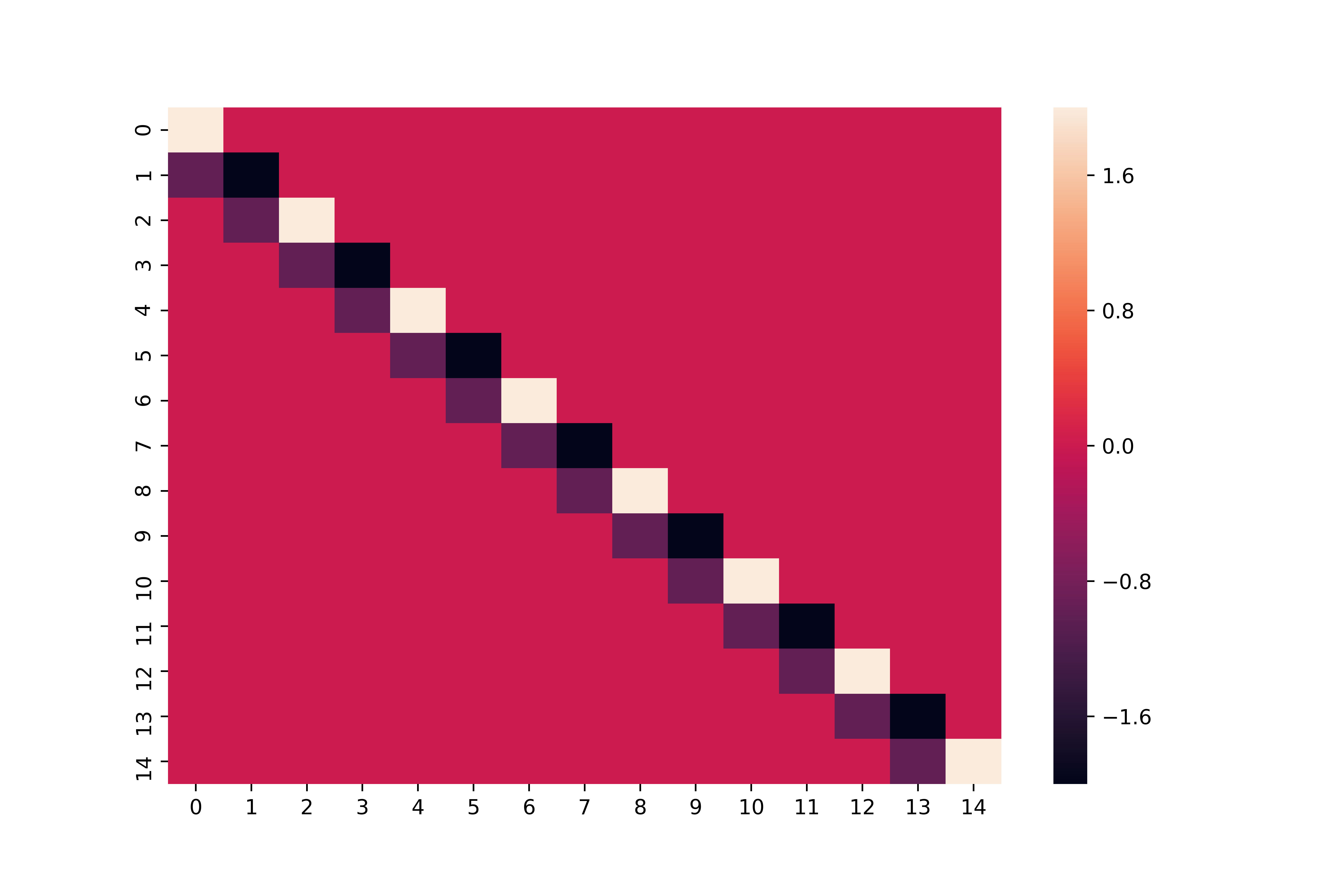
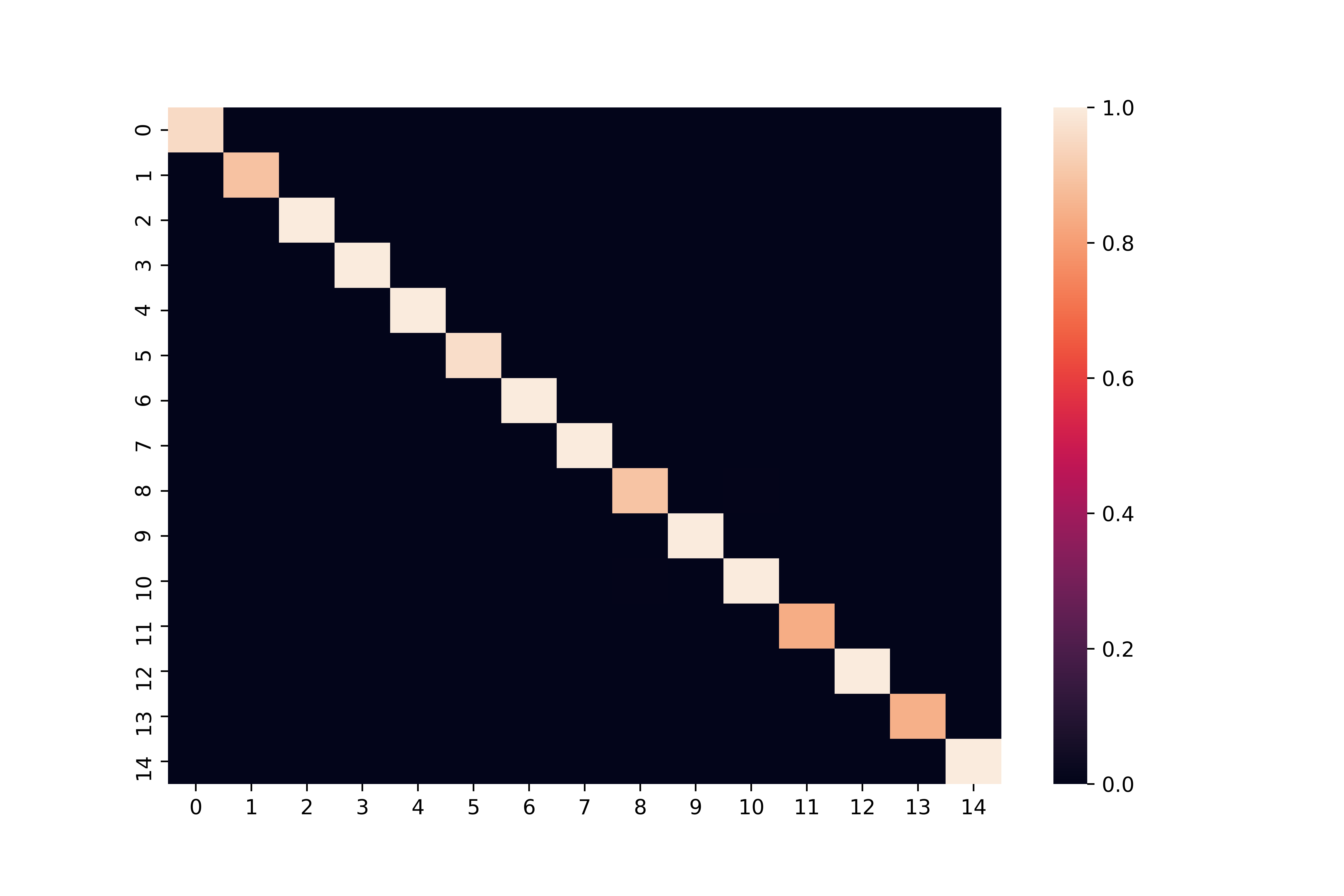
    ΔΔ\Delta-Diag: Δii=2.0(i=2n1)subscriptΔ𝑖𝑖2.0𝑖2𝑛1\Delta_{ii}=2.0\quad(i=2n-1), Δii=2.0(i=2n)subscriptΔ𝑖𝑖2.0𝑖2𝑛\Delta_{ii}=-2.0\quad(i=2n), otherwise 0.0.

  2. 2.

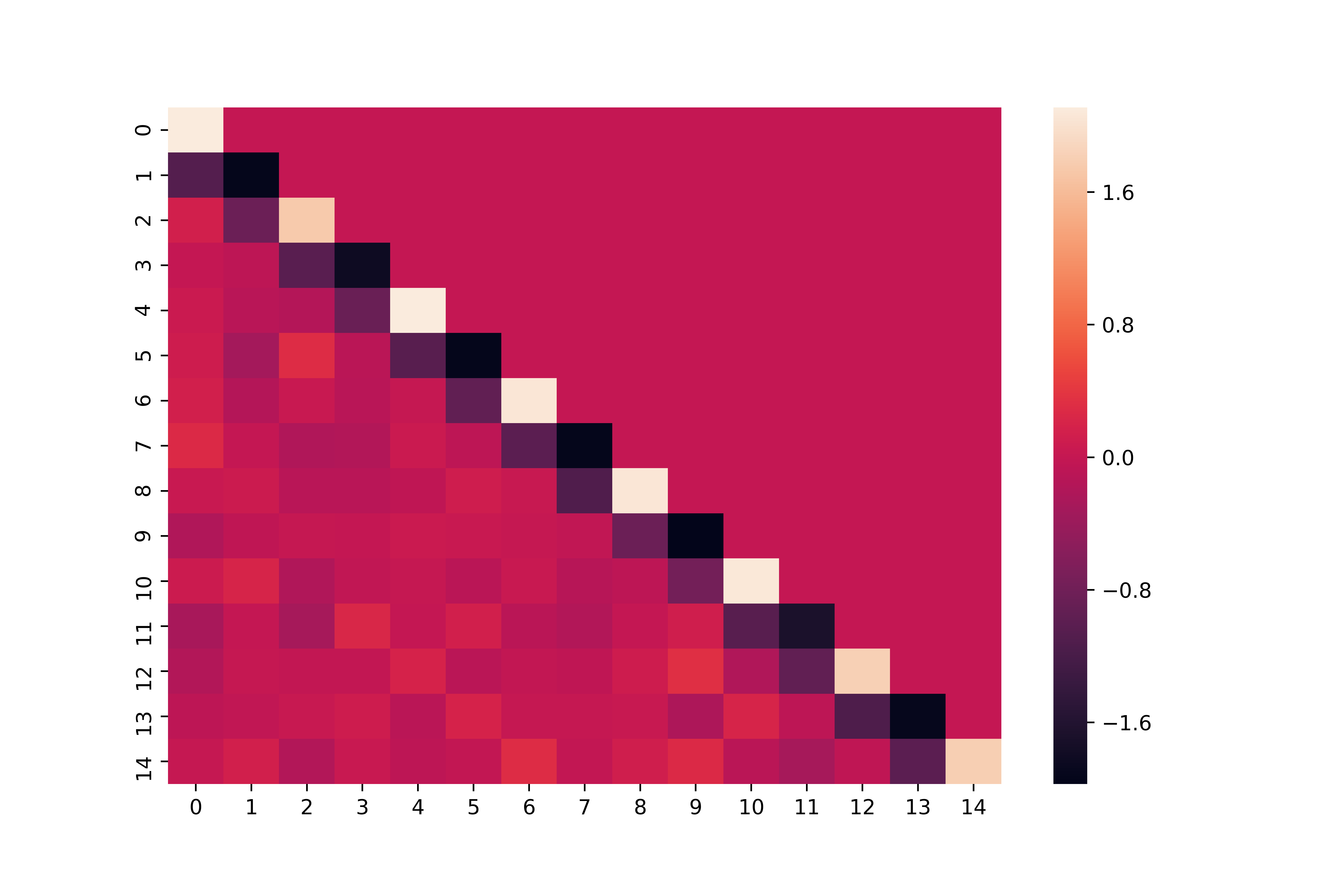
    ΔΔ\Delta-Sparse: Δii=2.0(i=2n1)subscriptΔ𝑖𝑖2.0𝑖2𝑛1\Delta_{ii}=2.0\quad(i=2n-1), Δii=2.0(i=2n)subscriptΔ𝑖𝑖2.0𝑖2𝑛\Delta_{ii}=-2.0\quad(i=2n) , Δi,i1=1.0subscriptΔ𝑖𝑖11.0\Delta_{i,i-1}=-1.0, otherwise 0.00.00.0.

  3. 3.

    ΔΔ\Delta-Dense: Δii=2.0(i=2n1)subscriptΔ𝑖𝑖2.0𝑖2𝑛1\Delta_{ii}=2.0\quad(i=2n-1), Δii=2.0(i=2n)subscriptΔ𝑖𝑖2.0𝑖2𝑛\Delta_{ii}=-2.0\quad(i=2n), Δi,i1=1.0subscriptΔ𝑖𝑖11.0\Delta_{i,i-1}=-1.0, otherwise the elements in lower-triangular equals to 1.0.

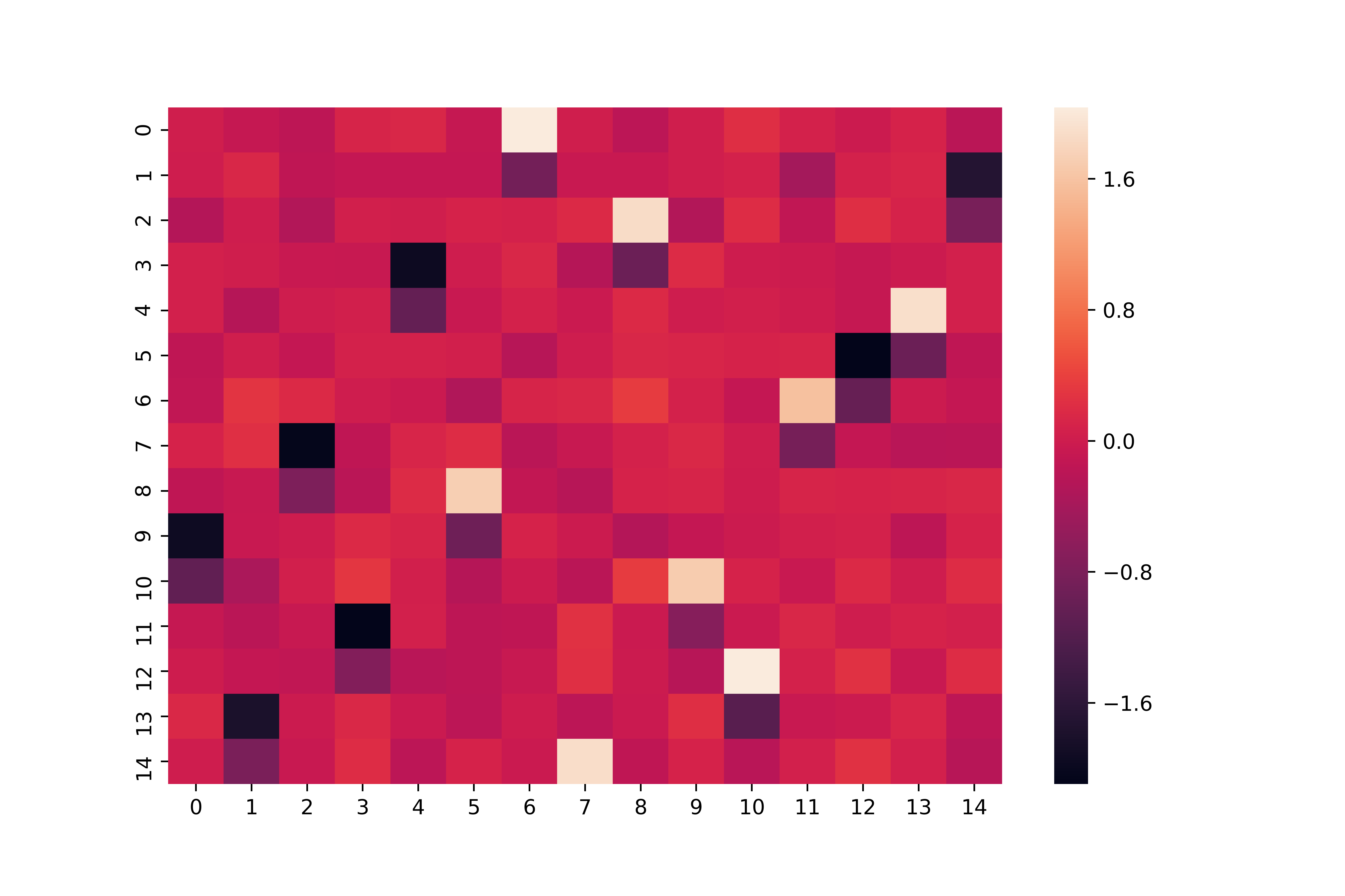
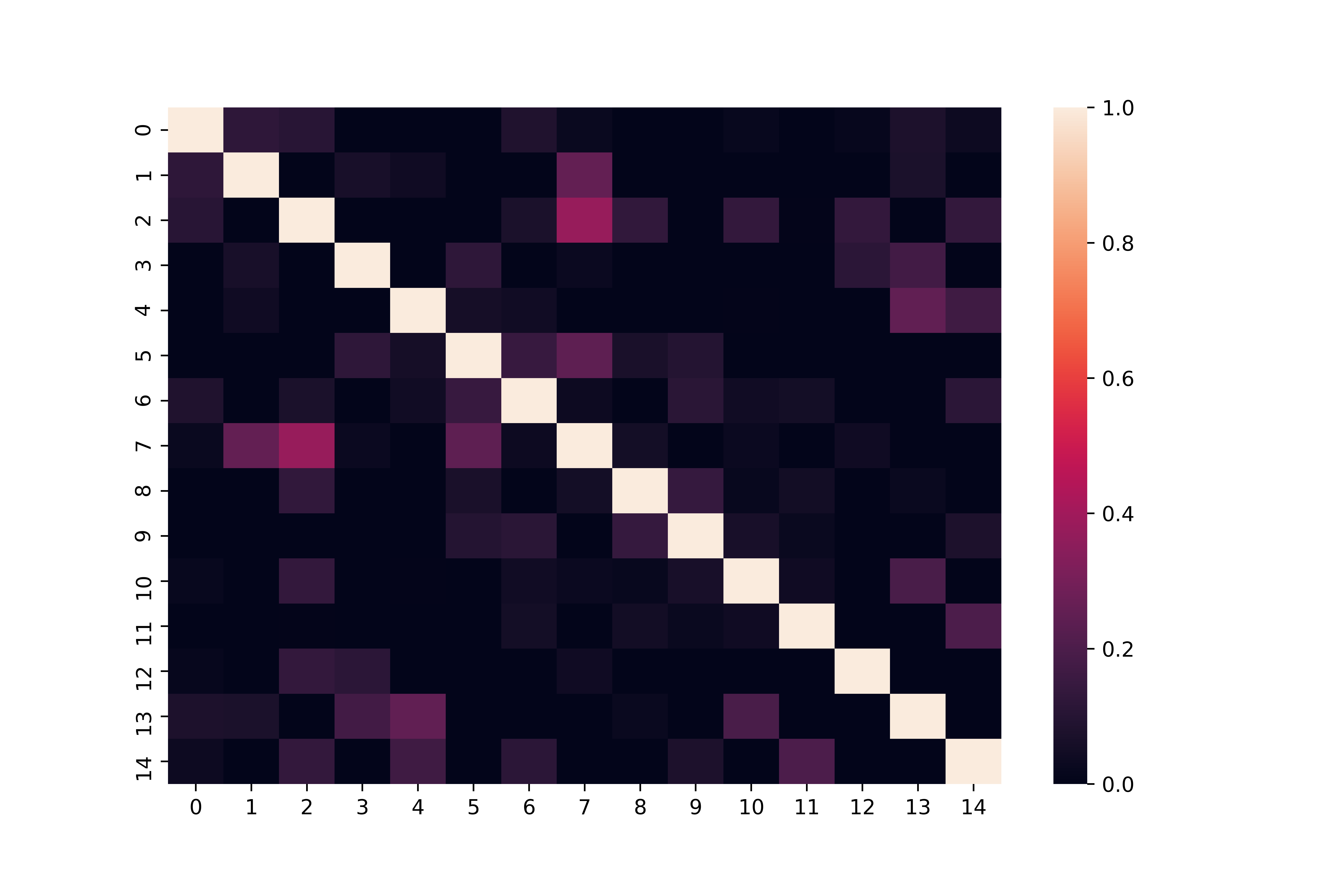
Since our main purpose is to compare estimation of ΔΔ\Delta, we set a simple assumption for the other parameter; ΩΩ\Omega is the identity matrix, μ𝜇\mu is fixed to zero. We generate artificial data of t = 1,500 and n = 15 from the multivariate skew-elliptical distribution with each specification and evaluate the posterior statistics of each parameter via MCMC. The hyper-parameters in the prior distributions are set up as follows.

Full-NOWI

bμ=0subscript𝑏𝜇0b_{\mu}=0, Aμ=0.01Isubscript𝐴𝜇0.01𝐼A_{\mu}=0.01I, bΔ=0subscript𝑏Δ0b_{\Delta}=0, AΔ=0.01Isubscript𝐴Δ0.01𝐼A_{\Delta}=0.01I, SΩ=nIsubscript𝑆Ω𝑛𝐼S_{\Omega}=nI, νΩ=nsubscript𝜈Ω𝑛\nu_{\Omega}=n in (6).

LT-NOWI

bμ=0subscript𝑏𝜇0b_{\mu}=0, Aμ=0.01Isubscript𝐴𝜇0.01𝐼A_{\mu}=0.01I, bδ=0subscript𝑏𝛿0b_{\delta}=0, Aδ=0.01Isubscript𝐴𝛿0.01𝐼A_{\delta}=0.01I, SΩ=nIsubscript𝑆Ω𝑛𝐼S_{\Omega}=nI, νΩ=nsubscript𝜈Ω𝑛\nu_{\Omega}=n in (15).

LT-HSGHS

bμ=0subscript𝑏𝜇0b_{\mu}=0, Aμ=0.01Isubscript𝐴𝜇0.01𝐼A_{\mu}=0.01I, bδ=0subscript𝑏𝛿0b_{\delta}=0, Aδ=0.01Isubscript𝐴𝛿0.01𝐼A_{\delta}=0.01I in (15); aη=1.0subscript𝑎𝜂1.0a_{\eta}=1.0 and bη=0.0subscript𝑏𝜂0.0b_{\eta}=0.0 in (29); Aω=0.01Isubscript𝐴𝜔0.01𝐼A_{\omega}=0.01I in (30)

In all cases, the number of burn-in iterations were 50,000, and the Monte Carlo sample from the following 100,000 iterations was used in the Bayesian inference. Also, we repeated simulations 30 times for each setup and obtained a set of point estimates of ΔΔ\Delta and ΩΩ\Omega. All computations are implemented with Python 3.7.0 on a desktop PC with 128GB RAM, 8GB GPU and eight-core 3.8GHz i7-10700K Intel processor.

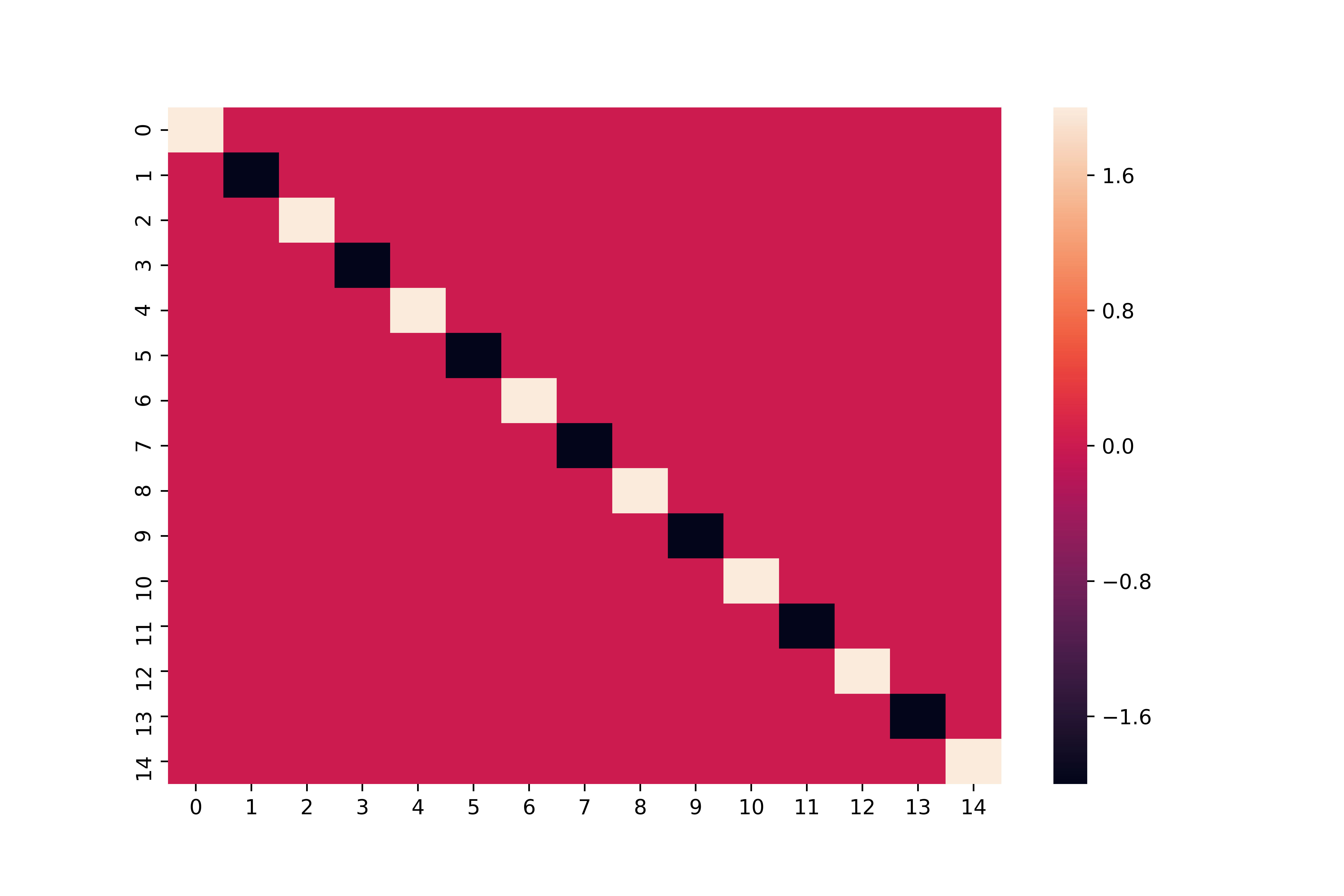
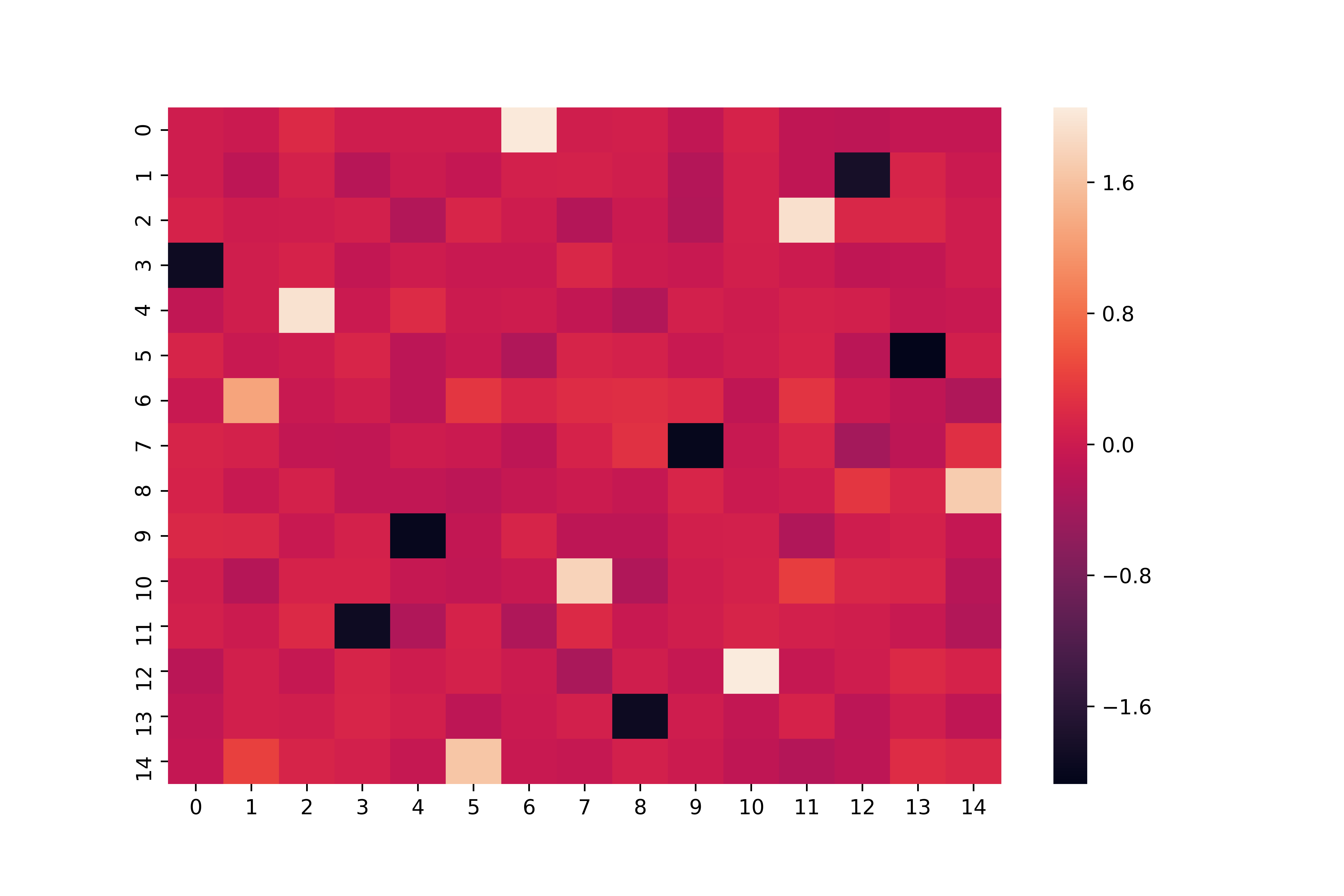
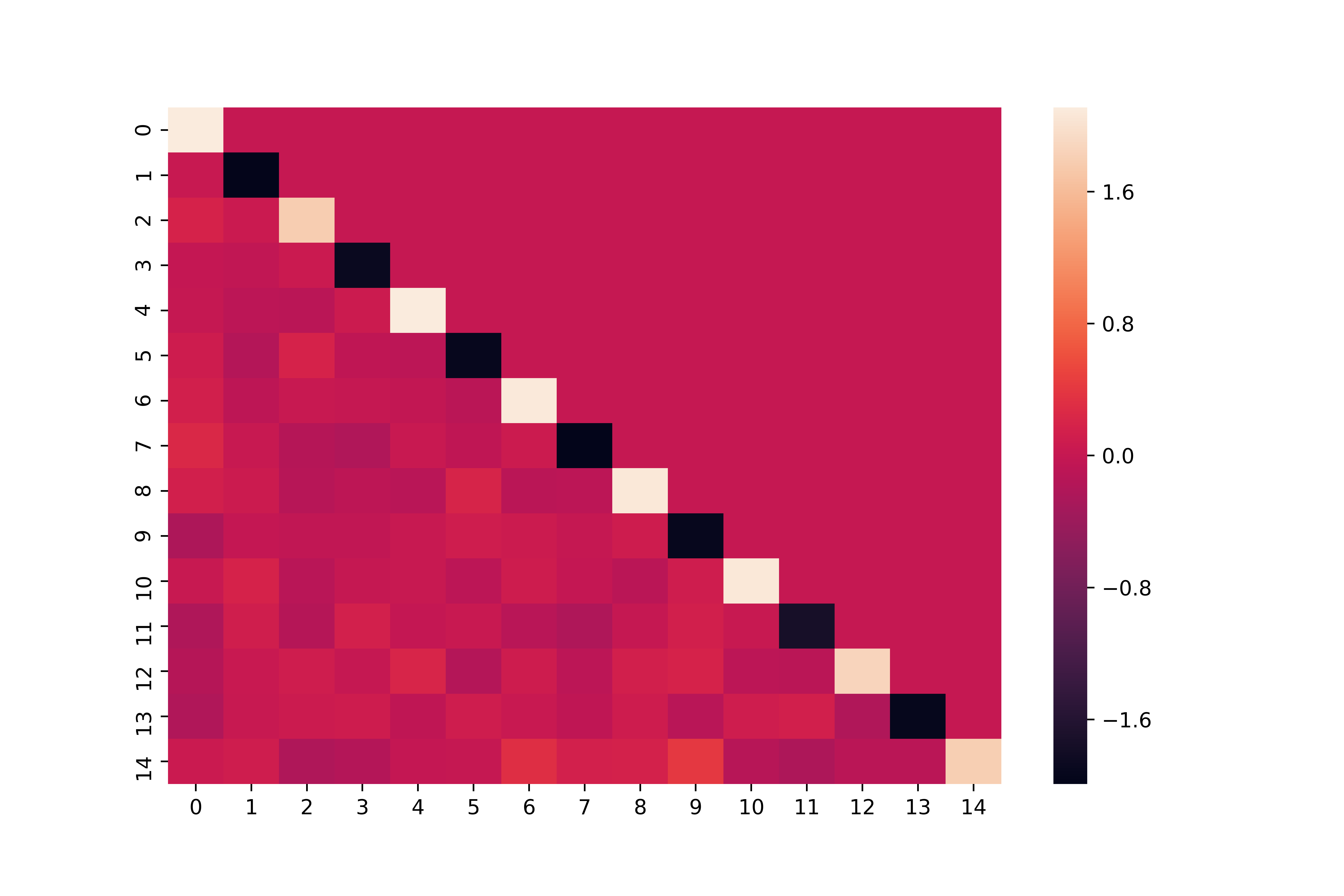
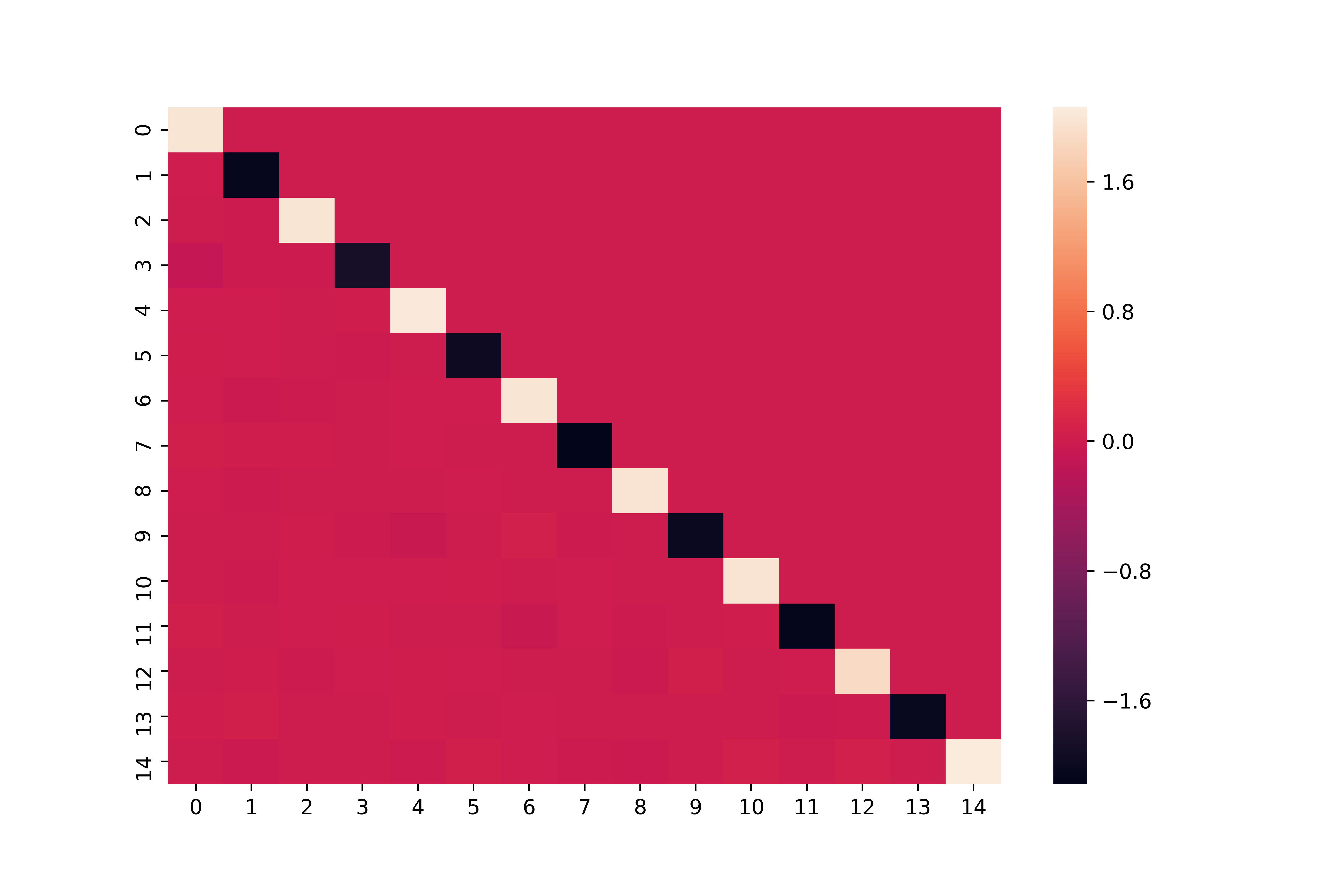
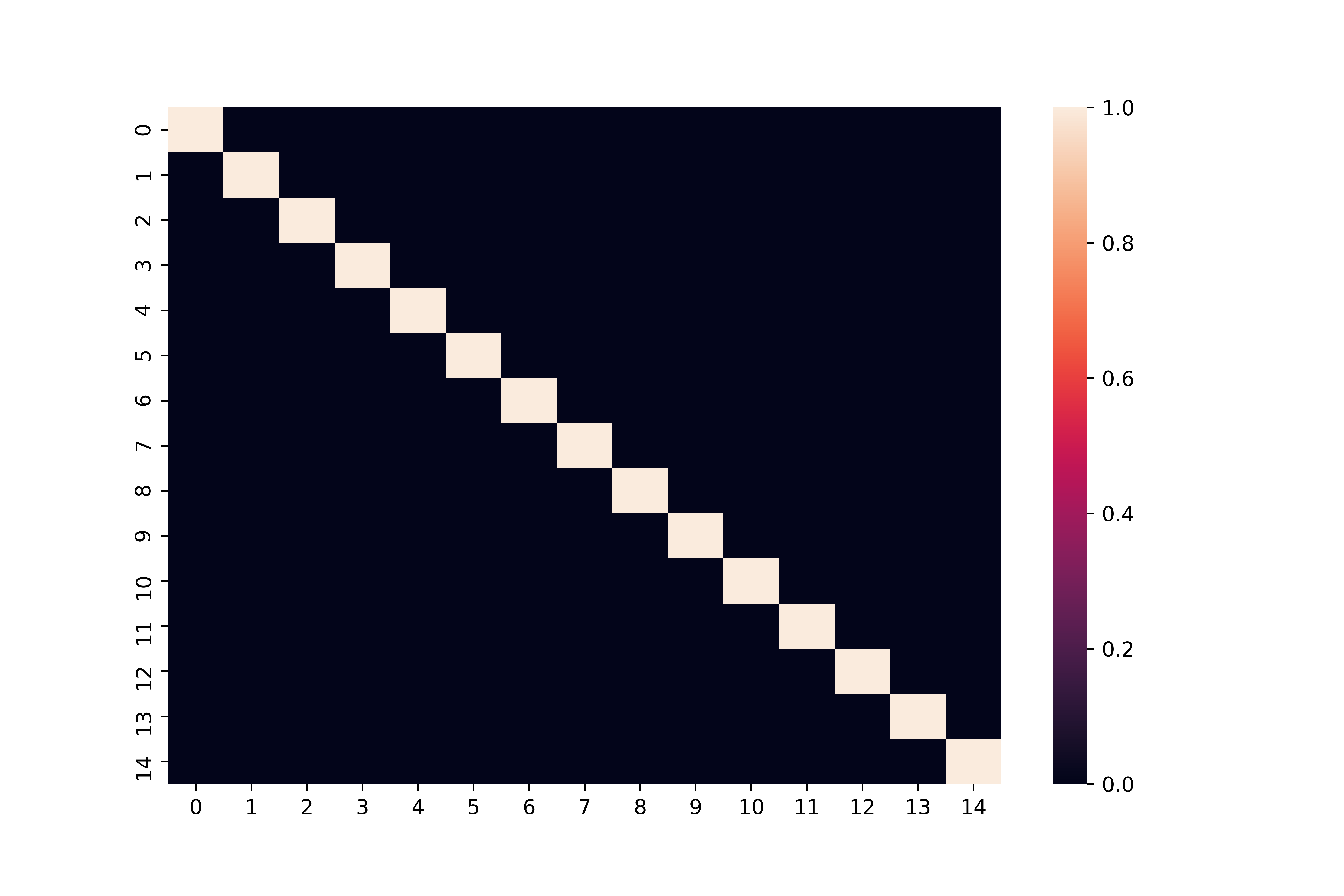
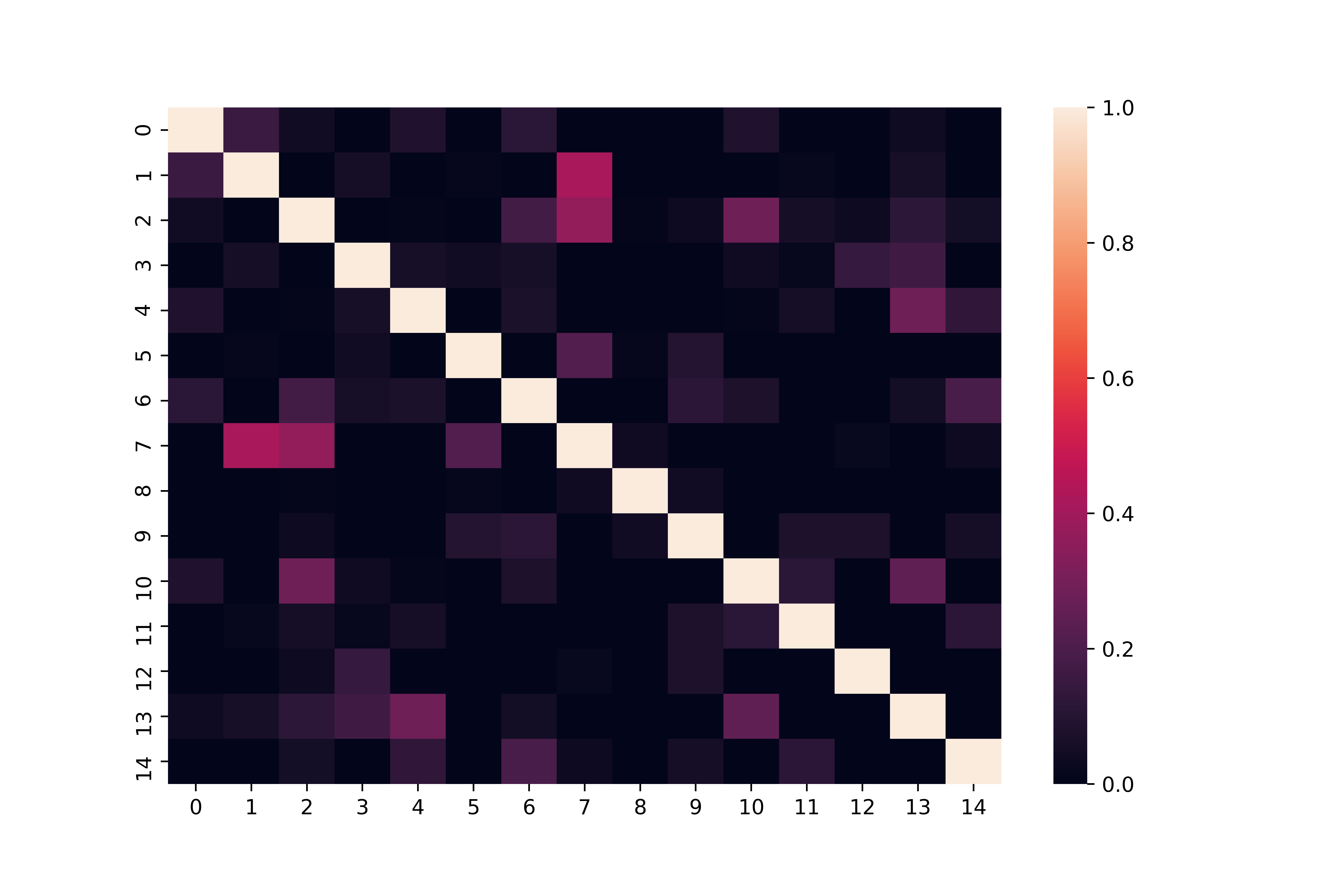
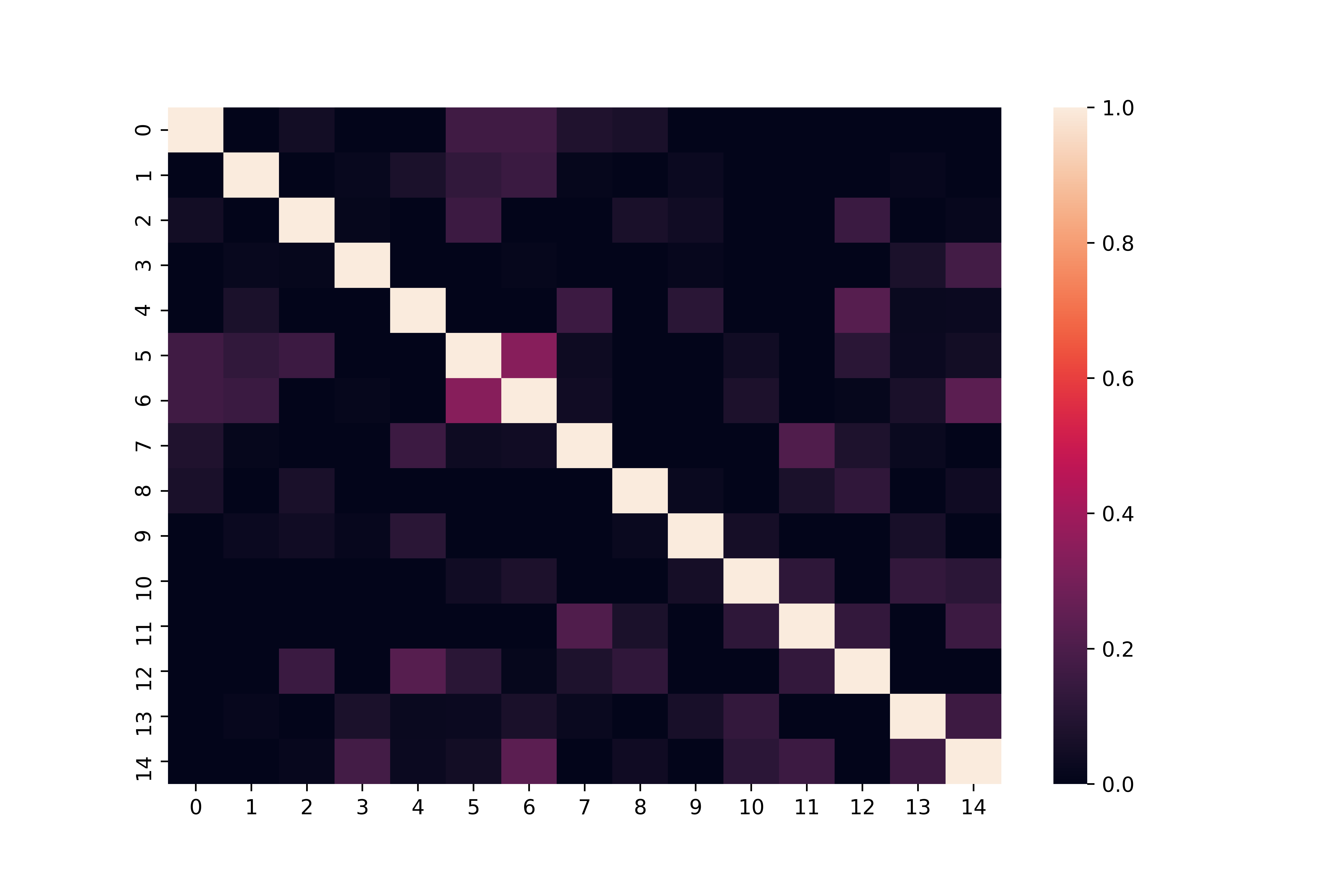
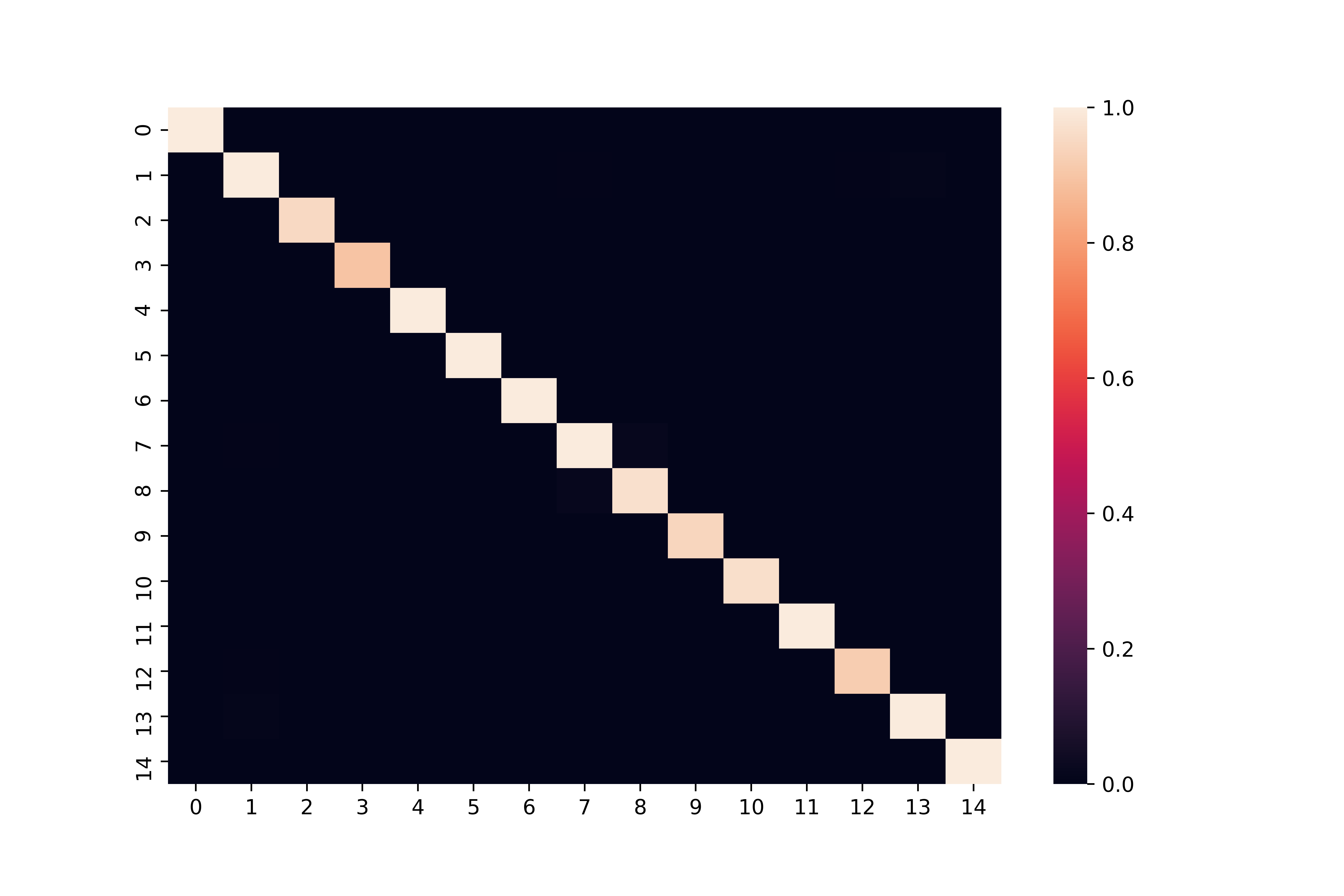
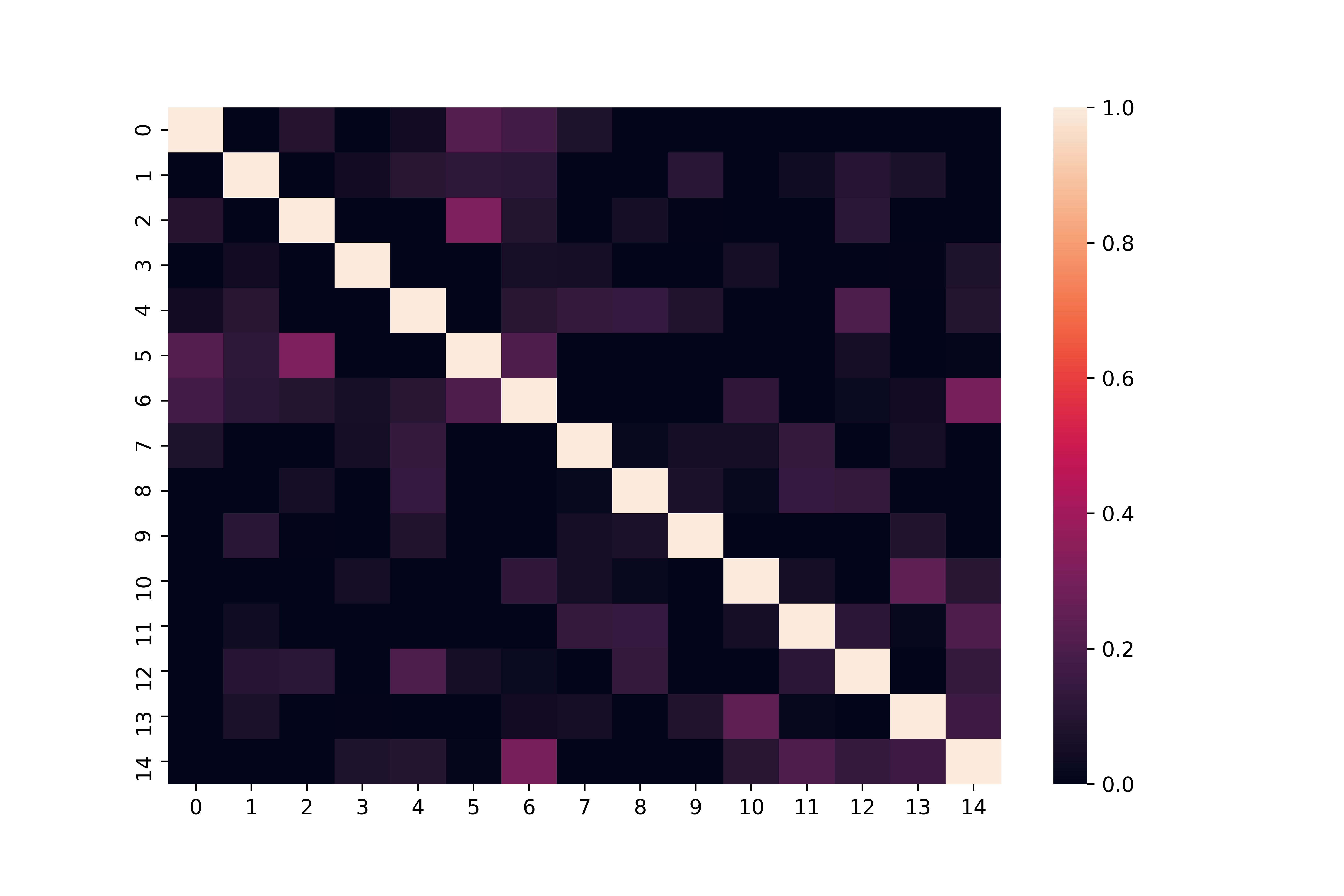
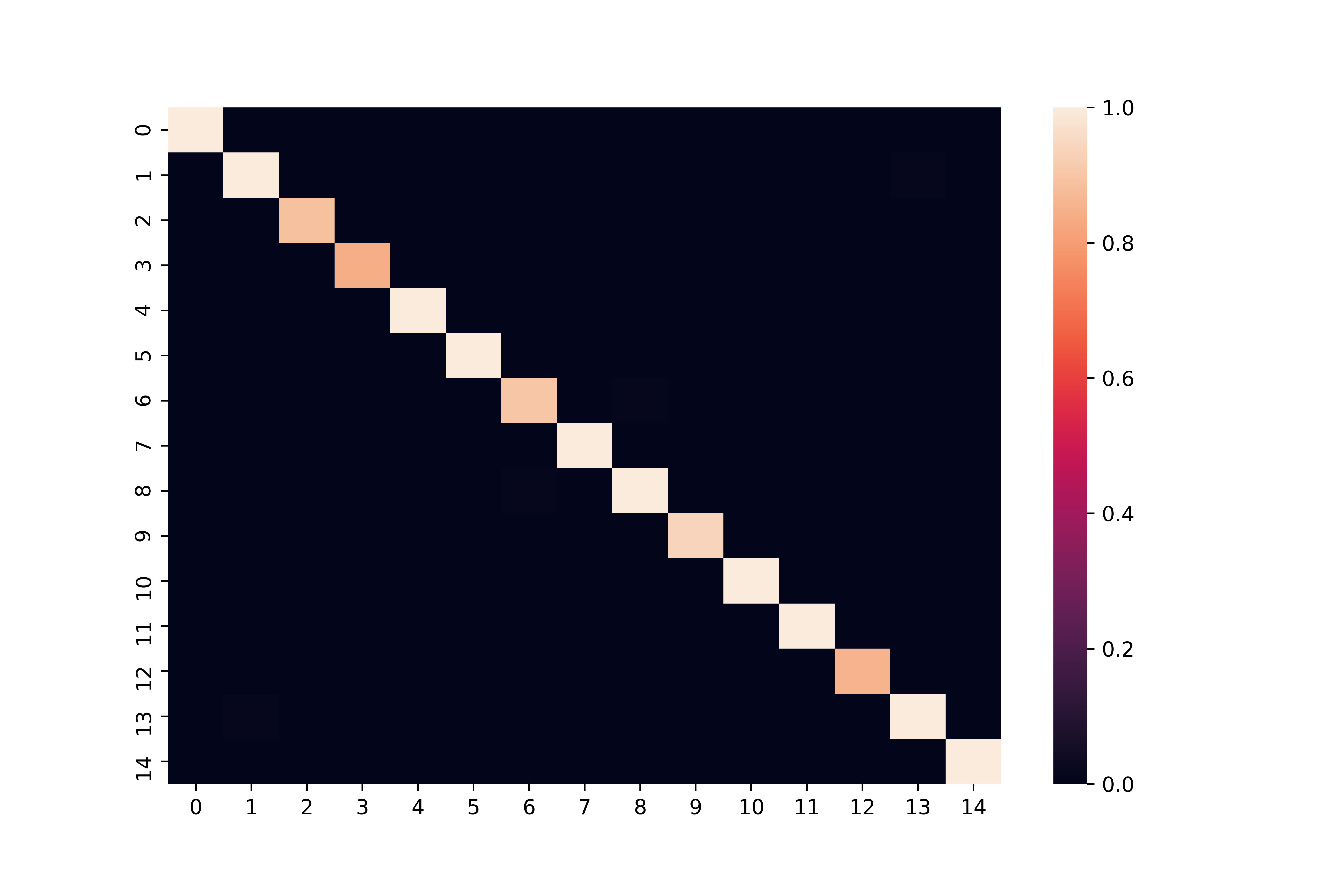
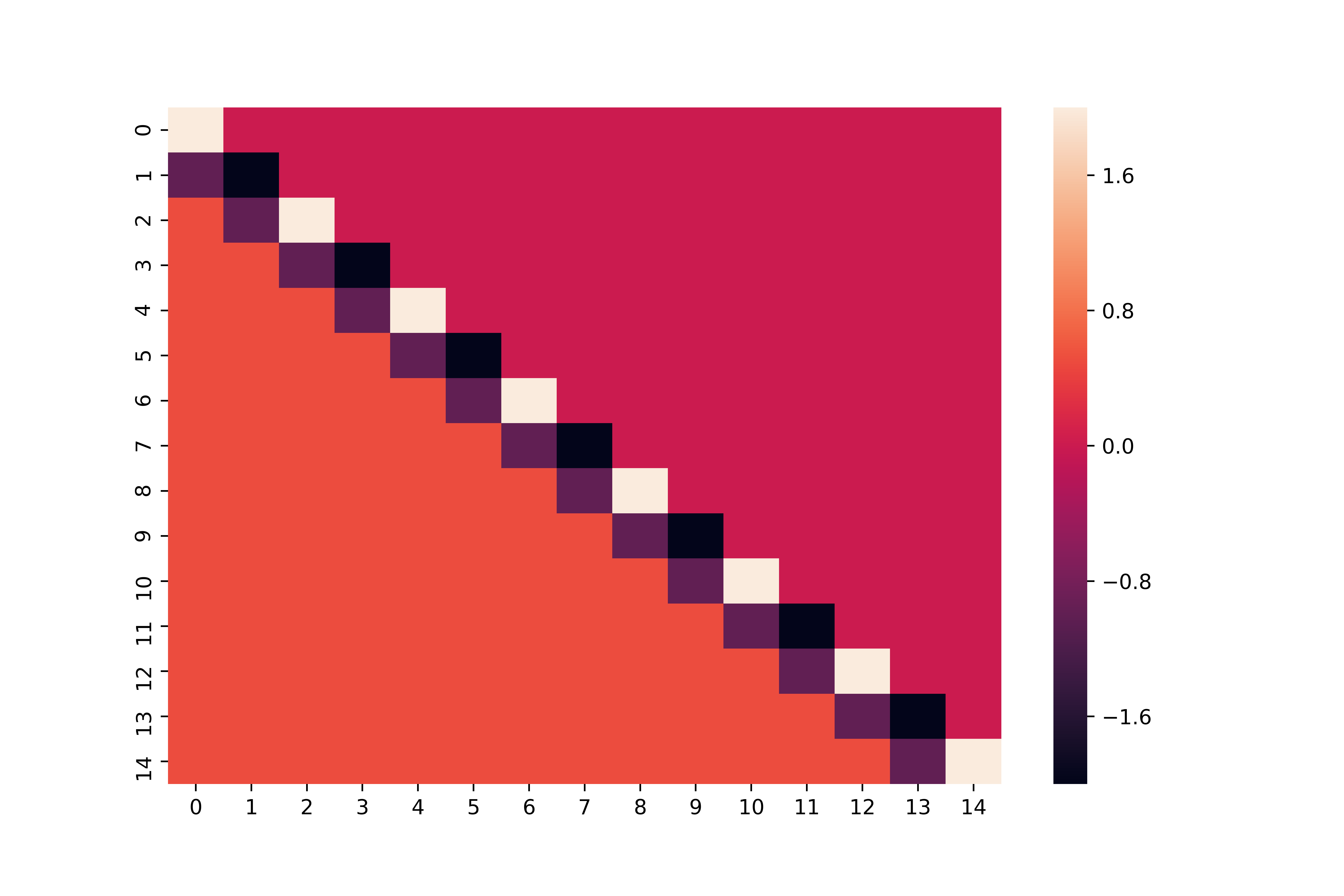
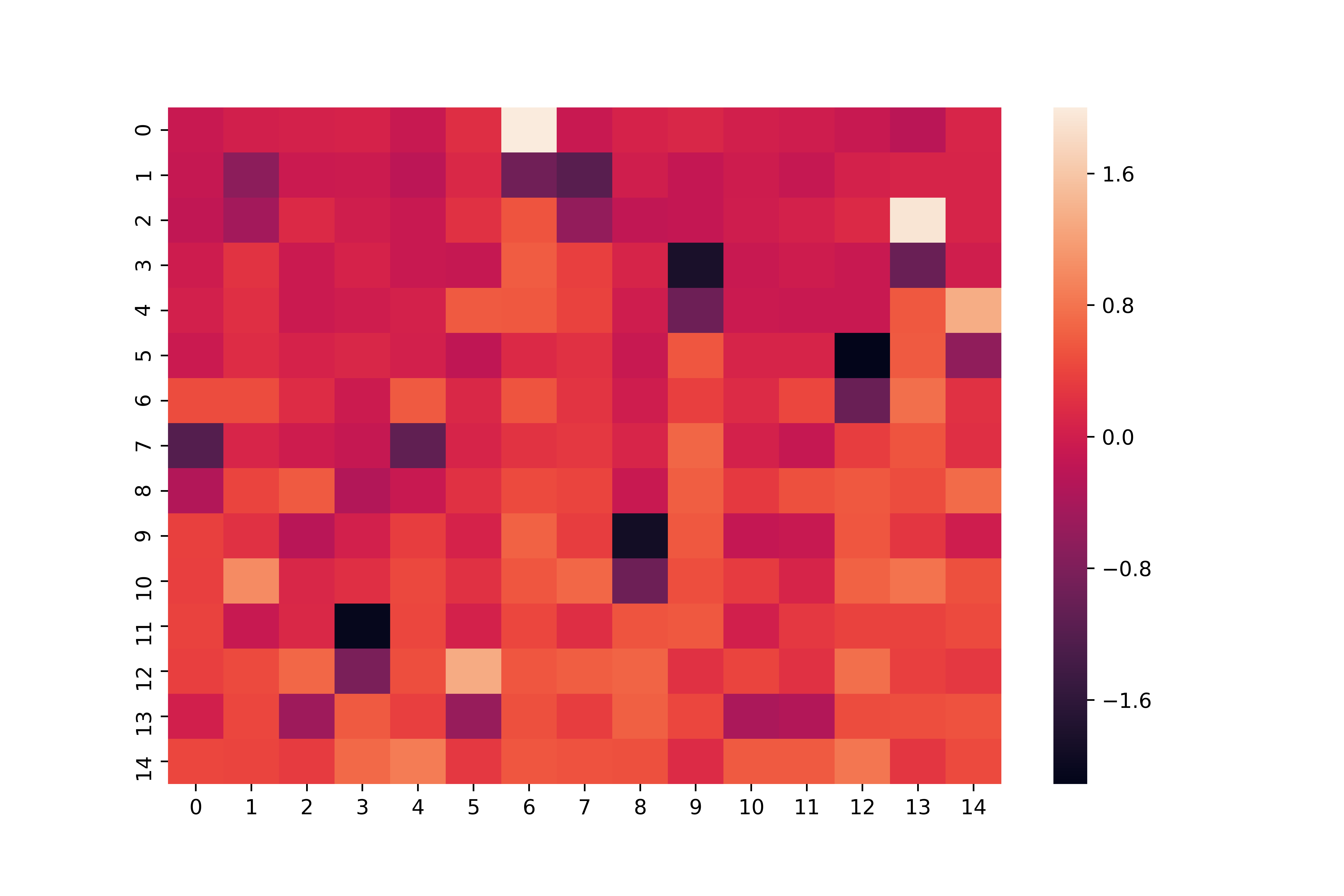
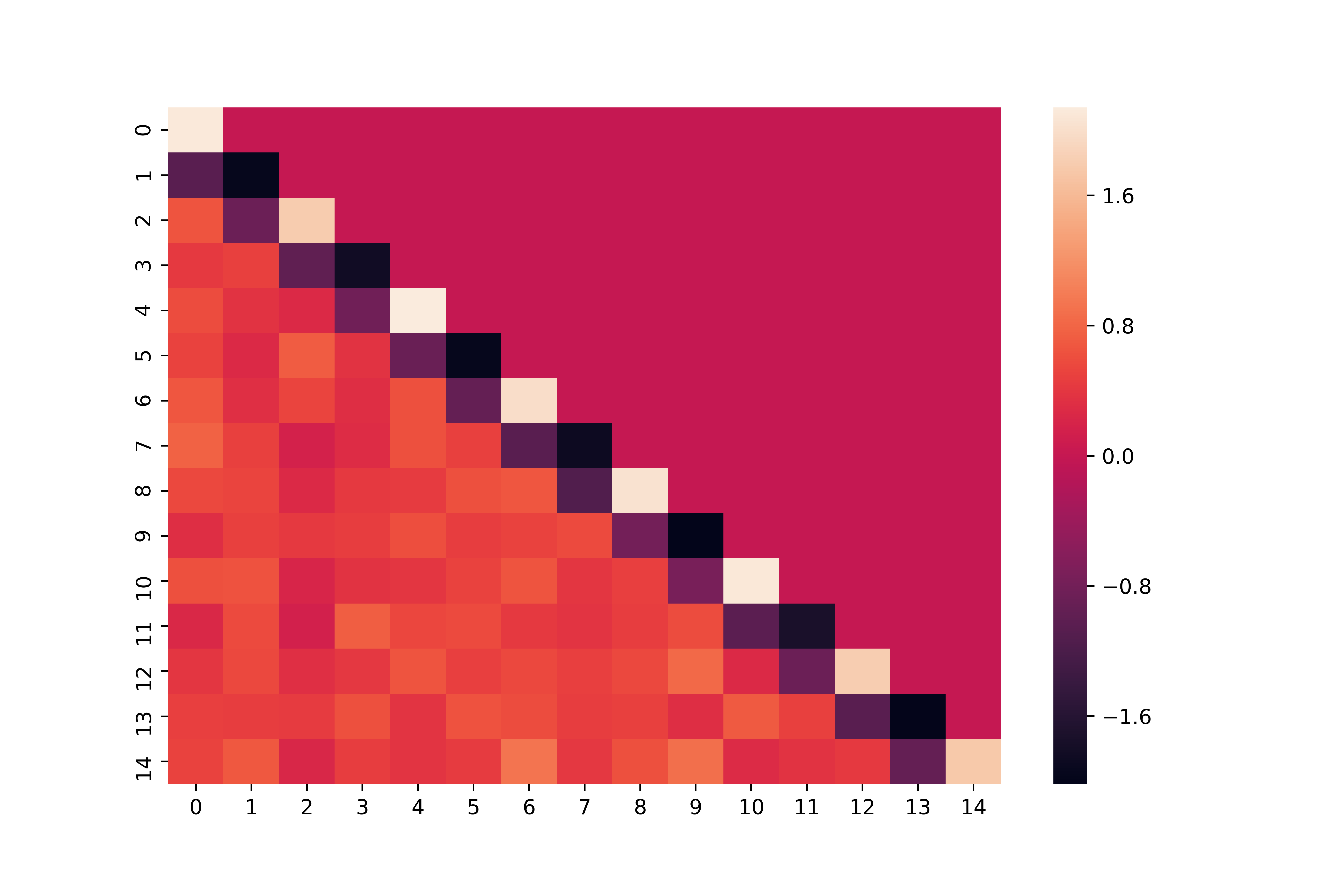
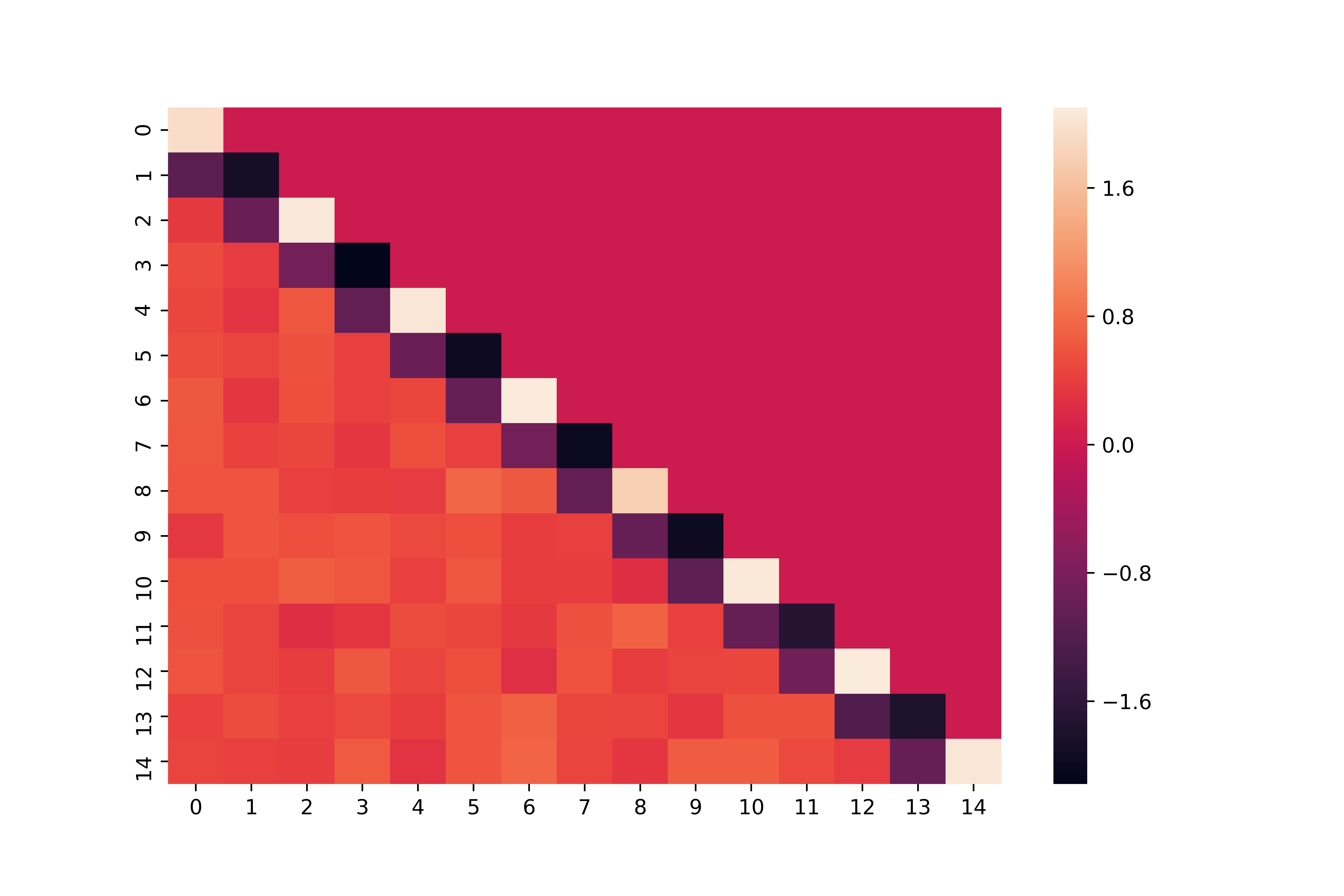
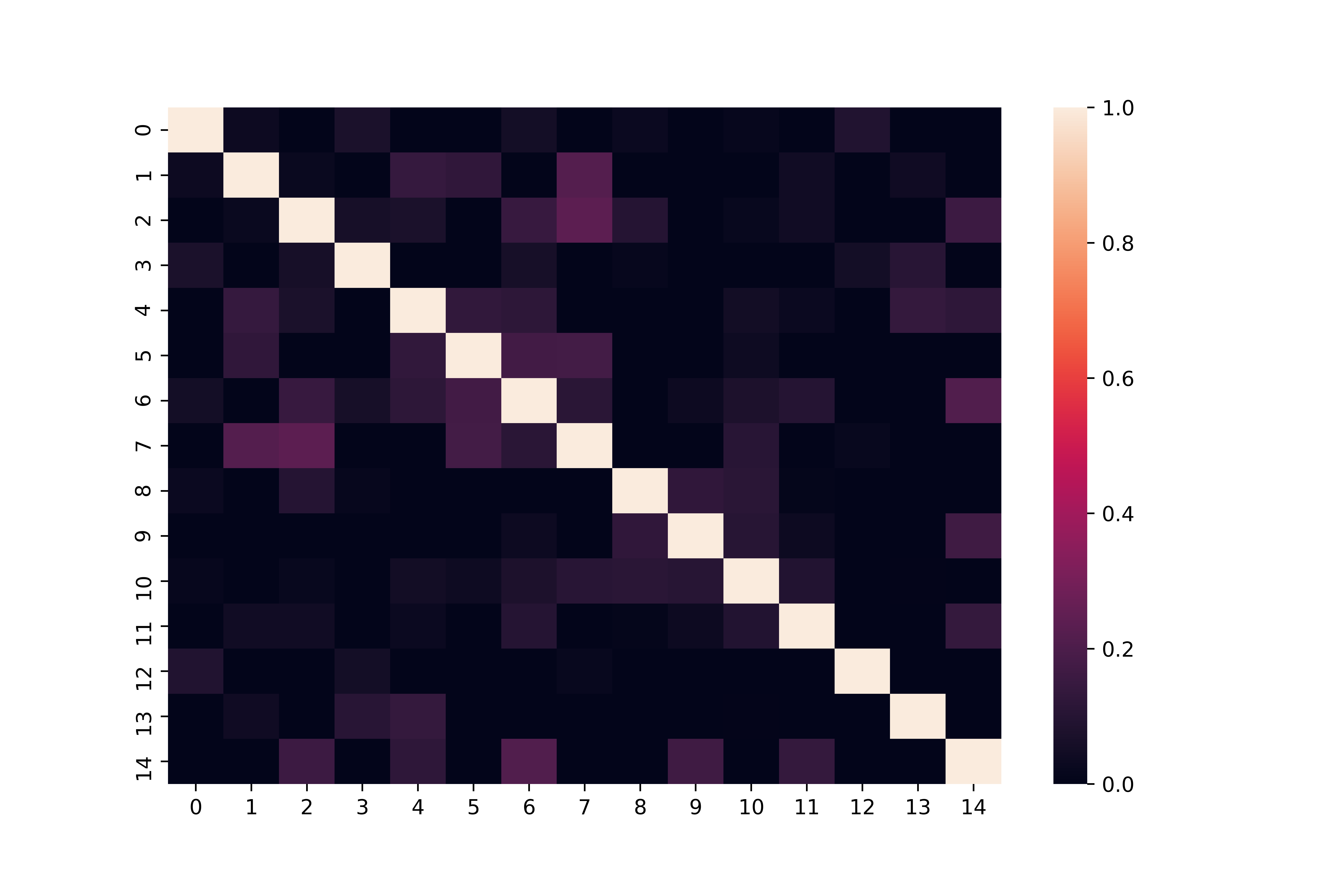
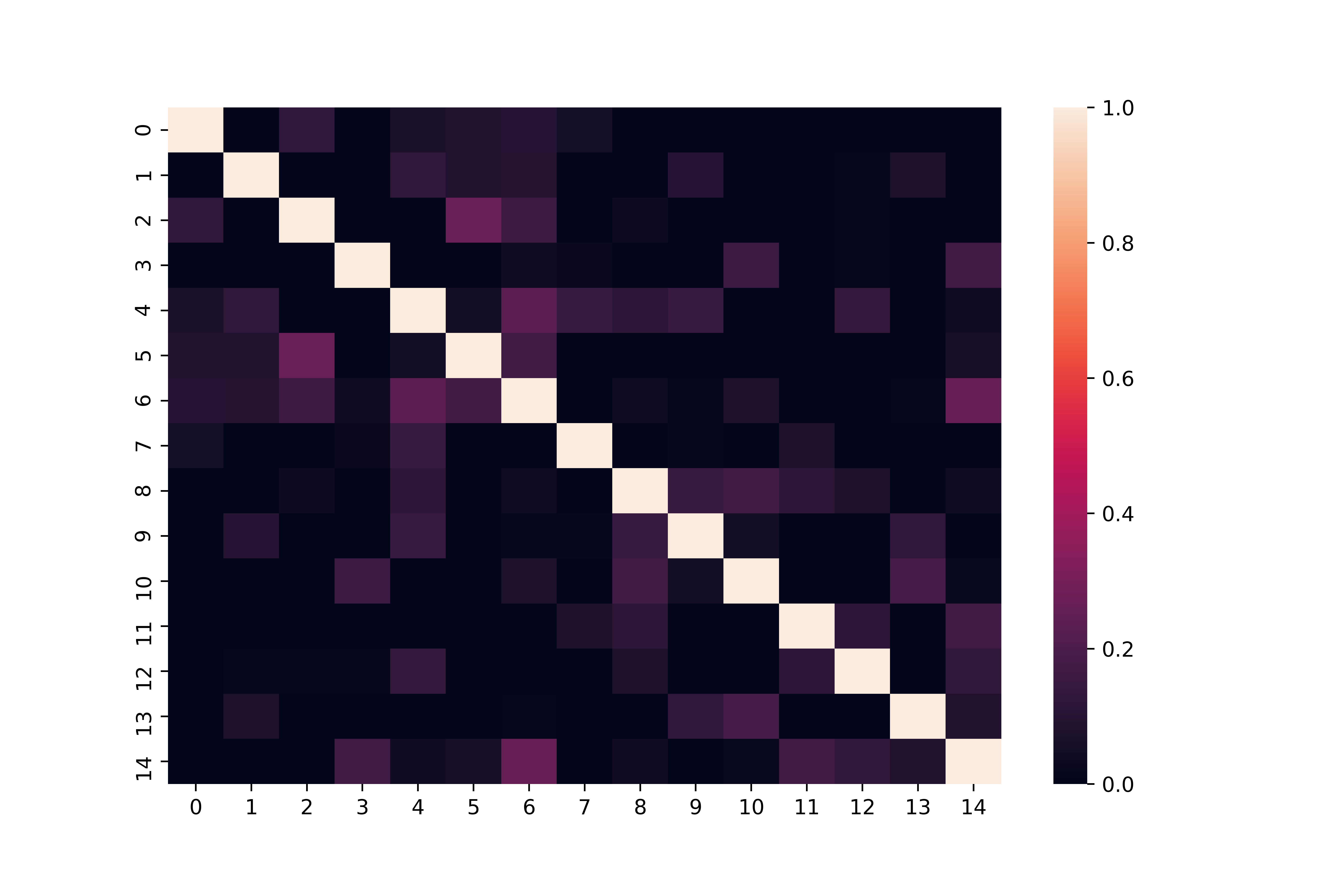
To compare the three models in terms of accuracy in the point estimation of ΔΔ\Delta and ΩΩ\Omega, we computed the Frobenius norm, as measurement of discrepancy between the point estimate and the true structure. Table 2 and 3 show the sample median loss with 30 replications for three models. The figures in parentheses are the standard errors. The smaller the value of the Frobenious norm, the closer the estimated structure is to the true one. In addition, in order to make the estimation results visually easy to understand, the posterior averages of ΔΔ\Delta and ΩΩ\Omega of each model in the 30th replication are shown in Figures 1 – 6.

First, regarding ΔΔ\Delta, the Frobenious norm of the proposed models (LT-NOWI, LT-HSGHS) have decreased to 1/8 or less of the Full-NOWI model for all designs and the estimation accuracy has remarkably improved in Table 2. This is because the columns of ΔΔ\Delta is not identified at all in Full-NOWI. On the other hand, this identification issue is resolved in LT-NOWI and LT-HSGHS and the structure of ΔΔ\Delta can be estimated well with the proposed method as shown in Figures 1, 3 and 5. Furthermore, for the ΔΔ\Delta-Diag case and the ΔΔ\Delta-Sparse case, Table 2 reports that the Frobenious norm of LT-HSGHS is less than half the value of LT-NOWI. This is because that the horseshoe prior in LT-HSGHS contributes to the estimation performance by shrinking non-essential elements to zero, while a large amount of non-zero entries still remain in ΔΔ\Delta for LT-NOWI as shown in Figures 1 and 3. However, the difference in the Frobenious norm between LT-NOWI and LT-HSGHS becomes smaller in the ΔΔ\Delta-Dense design because the sparse assumption of ΔΔ\Delta is not satisfied in this case.

Next, let take a look at results on ΩΩ\Omega. Note that the true structure of ΩΩ\Omega is the identity matrix. We examine how the estimation accuracy of ΩΩ\Omega changes across the structural designs of ΔΔ\Delta. For all designs of ΔΔ\Delta, the estimation accuracy is significantly improved in LT-HSGHS, the value of Frobenious norm is 1/3 or less in Table 3 compared with Full-NOWI and LT-NOWI. In fact, there are a lot of non-zero entries in the off-diagonal elements in Full-NOWI and LT-NOWI in Figures 2, 4 and 6. On the other hand, the posterior mean of ΩΩ\Omega in LT-HSGHS becomes the diagonal matrix thanks to the shrinkage effect. Also, comparing LT-NOWI with Full-NOWI, the Frobenious norm is slightly smaller in LT-NOWI for all ΔΔ\Delta designs. These findings suggest that the posterior distribution of ΩΩ\Omega is affected by the estimation of ΔΔ\Delta as shown in (10).

Table 2: Sample median loss in the point estimation of 𝚫𝚫\boldsymbol{\Delta}
ΔΔ\Delta-Diag ΔΔ\Delta-Sparse ΔΔ\Delta-Dense
Frobenius norm
Full-NOWI 10.587 11.588 12.620
(0.534) (0.743) (0.723)
LT-NOWI 1.344 1.362 1.420
(0.083) (0.115) (0.108)
LT-HSGHS 0.380 0.617 1.214
(0.070) (0.075) (0.138)
Notes: (a) The smaller losses are boldfaced.
(b) The figures in parentheses are the standard errors.
Table 3: Sample median loss in the point estimation of 𝛀𝛀\boldsymbol{\Omega}
ΔΔ\Delta-Diag ΔΔ\Delta-Sparse ΔΔ\Delta-Dense
Frobenius norm
Full-NOWI 2.550 2.447 2.352
(0.139) (0.138) (0.136)
LT-NOWI 2.255 2.238 2.210
(0.179) (0.147) (0.155)
LT-HSGHS 0.393 0.479 0.724
(0.101) (0.160) (0.288)
Notes: (a) The smaller losses are boldfaced.
(b) The figures in parentheses are the standard errors.
Refer to caption
(a) True
Refer to caption
(b) Full-NOWI
Refer to caption
(c) LT-NOWI
Refer to caption
(d) LT-HSGHS
Figure 1: ΔΔ\Delta-Diag: True Structure of ΔΔ\Delta and estimated ΔΔ\Delta
Refer to caption
(a) True
Refer to caption
(b) Full-NOWI
Refer to caption
(c) LT-NOWI
Refer to caption
(d) LT-HSGHS
Figure 2: ΔΔ\Delta-Diag: True Structure of ΩΩ\Omega and estimated ΩΩ\Omega
Refer to caption
(a) True
Refer to caption
(b) Full-NOWI
Refer to caption
(c) LT-NOWI
Refer to caption
(d) LT-HSGHS
Figure 3: ΔΔ\Delta-Sparse: True Structure of ΔΔ\Delta and estimated ΔΔ\Delta
Refer to caption
(a) True
Refer to caption
(b) Full-NOWI
Refer to caption
(c) LT-NOWI
Refer to caption
(d) LT-HSGHS
Figure 4: ΔΔ\Delta-Sparse: True Structure of ΩΩ\Omega and estimated ΩΩ\Omega
Refer to caption
(a) True
Refer to caption
(b) Full-NOWI
Refer to caption
(c) LT-NOWI
Refer to caption
(d) LT-HSGHS
Figure 5: ΔΔ\Delta-Dense: True Structure of ΔΔ\Delta and estimated ΔΔ\Delta
Refer to caption
(a) True
Refer to caption
(b) Full-NOWI
Refer to caption
(c) LT-NOWI
Refer to caption
(d) LT-HSGHS
Figure 6: ΔΔ\Delta-Dense: True Structure of ΩΩ\Omega and estimated ΩΩ\Omega

4 Conclusion

In this paper, we have raised a possible identification issue on the skewness matrix of the skew-elliptical distribution in the Bayesian MCMC method proposed by Harvey et al. (2010) due to label switching. To avoid this issue, we proposed an modified model in which the lower-triangular constraint was imposed upon the skewness matrix. Moreover, we devised an extended model with the horseshoe prior for both skewness matrix and precision matrix to further improve the estimation accuracy.

In the simulation study, we compared the proposed models with the model of Harvey et al. (2010) in the three structural designs of the skewness matrix and found that the proposed models with the identification constraint significantly improved the estimation accuracy of the skewness matrix.

Acknowledgements

This research is supported by the Keio University Doctorate Student Grant-in-Aid Program from Ushioda Memorial Fund; and JSPS KAKENHI under Grant [number MKK337J].

Conflict of interest

The authors declare that they are funded by the Keio University Doctorate Student Grant-in-Aid Program from Ushioda Memorial Fund and JSPS KAKENHI under Grant [number MKK337J] to conduct this research.

Ethical standards

The authors declare that the experiments in this paper comply with the current laws of Japan where we had conducted the experiment.

References

  • Aas and Haff (2006) K. Aas and I. H. Haff. The generalized hyperbolic skew student’s t-distribution. Journal of Financial Econometrics, 4(2):275–309, 2006.
  • Adcock and Azzalini (2020) C. Adcock and A. Azzalini. A selective overview of skew-elliptical and related distributions and of their applications. Symmetry, 12(1), 2020.
  • Alodat and Al-Rawwash (2014) M. T. Alodat and M. Y. Al-Rawwash. The extended skew gaussian process for regression. METRON, 72(3):317–330, 2014.
  • Azzalini and Capitanio (2003) A. Azzalini and A. Capitanio. Distributions generated by perturbation of symmetry with emphasis on a multivariate skew t-distribution. Journal of the Royal Statistical Society: Series B (Statistical Methodology), 65(2):367–389, 2003.
  • Azzalini and Valle (1996) A. Azzalini and D. Valle. The multivariate skew-normal distribution. Biometrika, 83(4):715–726, 1996.
  • Barbi and Romagnoli (2018) M. Barbi and S. Romagnoli. Skewness, basis risk, and optimal futures demand. International Review of Economics & Finance, 58:14–29, 2018.
  • Barndorff-Nielsen (1977) O. E. Barndorff-Nielsen. Exponentially decreasing distributions for the logarithm of particle size. Proceedings of the Royal Society of London. A. Mathmatical and Physical Sciences, 353:401–419, 1977.
  • Bélisle et al. (1993) C. J. P. Bélisle, H. E. Romeijn, and R. L. Smith. Hit-and-run algorithms for generating multivariate distributions. Mathmatics of Operations Research, 18(2):255–266, 1993.
  • Branco and Dey (2001) M. D. Branco and D. K. Dey. A general class of multivariate skew-elliptical distributions. Journal of Multivariate Analysis, 79(1):99–113, 2001.
  • Carmichael and Coën (2013) B. Carmichael and A. Coën. Asset pricing with skewed-normal return. Finance Research Letters, 10(2):50–57, 2013.
  • Carvalho et al. (2010) C. M. Carvalho, N. G. Polson, and J. G. Scott. The horseshoe estimator for sparse signals. Biometrika, 97(2):465–480, 2010.
  • Fernández and Steel (1998) C. Fernández and M. F. J. Steel. On bayesian modeling of fat tails and skewness. Journal of the American Statistical Association, 93(441):359–371, 1998.
  • Frühwirth-Schnatter and Lopes (2018) S. Frühwirth-Schnatter and H. F. Lopes. Sparse bayesian factor analysis when the number of factors is unknown. arXiv: 1804.04231, 2018.
  • Geweke and Zhou (1996) J. Geweke and G. Zhou. Measuring the pricing error of the arbitrage pricing theory. The Review of Financial Studies, 9(2):557–587, 1996.
  • Hansen (1994) B. E. Hansen. Autoregressive conditional density estimation. International Economic Review, 35(3):705–730, 1994.
  • Harvey et al. (2010) C. R. Harvey, J. C. Liechty, M. W. Liechty, and P. Müller. Portfolio selection with higher moments. Quantitative Finance, 10(5):469–485, 2010.
  • Kon (1984) S. J. Kon. Models of stock returns—a comparison. The Journal of Finance, 39(1):147–165, 1984.
  • Li et al. (2019) Y. Li, B. A. Craig, and A. Bhadra. The graphical horseshoe estimator for inverse covariance matrices. Journal of Computational and Graphical Statistics, 28(3):747–757, 2019.
  • Lopes and West (2004) H. F. Lopes and M. West. Bayesian model assessment in factor analysis. Statistica Sinica, 14(1):41–67, 2004.
  • Makalic and Schmidt (2016) E. Makalic and D. F. Schmidt. A simple sampler for the horseshoe estimator. IEEE Signal Processing Letters, 23(1):179–182, 2016.
  • Markowitz (1952) H. Markowitz. Portfolio selection. Journal of Finance, 7(1):77–91, 1952.
  • Markowitz and Usmen (1996) H. Markowitz and N. Usmen. The likelihood of various stock market return distributions, part 2: Empirical results. Journal of Risk and Uncertainty, 13(3):221–247, 1996.
  • Mills (1995) T.C. Mills. Modelling skewness and kurtosis in the london stock exchange ft-se index return distributions. Journal of the Royal Statistical Society: Series D (The Statistician), 44(3):323–332, 1995.
  • Nakajima (2017) J. Nakajima. Bayesian analysis of multivariate stochastic volatility with skew return distribution. Econometric Reviews, 36(5):546–562, 2017.
  • Nakajima and Omori (2012) J. Nakajima and Y. Omori. Stochastic volatility model with leverage and asymmetrically heavy-tailed error using gh skew student’s t-distribution. Computational Statistics & Data Analysis, 56(11):3690–3704, 2012.
  • Oya and Nakatsuma (2021) S. Oya and T. Nakatsuma. A positive-definiteness-assured block gibbs sampler for bayesian graphical models with shrinkage priors. arXiv:2001.04657v2, 2021.
  • Panagiotelis and Smith (2010) A. Panagiotelis and M. Smith. Bayesian skew selection for multivariate models. Computational Statistics & Data Analysis, 54(7):1824–1839, 2010.
  • Peiró (1999) A. Peiró. Skewness in financial returns. Journal of Banking & Finance, 23(6):847–862, 1999.
  • Sahu et al. (2003) S. K. Sahu, D. K. Dey, and M.D. Branco. A new class of multivariate skew distributions with applications to bayesian regression models. Canadian Journal of Statistics, 31(2):129–150, 2003.
  • Wang (2012) H. Wang. Bayesian graphical lasso methods and efficient posterior computation. Bayesian Analysis, 7:867–886, 2012.
  • Watanabe (2001) T. Watanabe. On sampling the degree-of-freedom of student’s-t disturbances. Statistics & Probability Letters, 52(2):177–181, 2001.
  • West (2003) M. West. Bayesian factor regression models in the “large p, small n” paradigm. Bayesian Statistics, 7:733–742, 2003.

Appendix

As we mentioned before, Harvey et al. (2010) developed the Gibbs sampling algorithm for the multivariate skew-normal distribution (1), but it is straightforward to extend it to the multivariate skew-t distribution as Sahu et al. (2003) showed. Since it is expressed as a scale mixture of multivariate skew-normal distributions, skew-t distributed Rtsubscript𝑅𝑡R_{t} is expressed as

Rt=μ+ΔZt+ϵt,Zt𝒩+(0,1γtIN),ϵt𝒩(0,(γtΩ)1),γtGa(φ2,φ2),Ztϵtγt,\begin{split}&R_{t}=\mu+\Delta Z_{t}+\epsilon_{t},\\ &Z_{t}\sim\mathcal{N}^{+}\left(0,\frac{1}{\gamma_{t}}I_{N}\right),\quad\epsilon_{t}\sim\mathcal{N}\left(0,\left(\gamma_{t}\Omega\right)^{-1}\right),\quad\gamma_{t}\sim Ga\left(\frac{\varphi}{2},\frac{\varphi}{2}\right),\\ &Z_{t}\perp\epsilon_{t}\perp\gamma_{t},\end{split} (37)

Given γtsubscript𝛾𝑡\gamma_{t}, the sampling algorithms for δ𝛿\delta, ΩΩ\Omega, μ𝜇\mu and Ztsubscript𝑍𝑡Z_{t} in (37) are almost identical to the multivariate skew-normal case except that

δ𝛿\delta:

redefine A^δsubscript^𝐴𝛿\hat{A}_{\delta} and b^δsubscript^𝑏𝛿\hat{b}_{\delta} in (16) as

A^δ=Aδ+t=1TγtWtΩWt,b^δ=Aδbδ+t=1TγtWtΩR~t.formulae-sequencesubscript^𝐴𝛿subscript𝐴𝛿superscriptsubscript𝑡1𝑇subscript𝛾𝑡superscriptsubscript𝑊𝑡Ωsubscript𝑊𝑡subscript^𝑏𝛿subscript𝐴𝛿subscript𝑏𝛿superscriptsubscript𝑡1𝑇subscript𝛾𝑡superscriptsubscript𝑊𝑡Ωsubscript~𝑅𝑡\hat{A}_{\delta}=A_{\delta}+\sum_{t=1}^{T}\gamma_{t}W_{t}^{\intercal}\Omega W_{t},\quad\hat{b}_{\delta}=A_{\delta}b_{\delta}+\sum_{t=1}^{T}\gamma_{t}W_{t}^{\intercal}\Omega\tilde{R}_{t}.
ΩΩ\Omega:

redefine S𝑆S in (10) as

S=t=1Tγt(RtμΔZt)(RtμΔZt).𝑆superscriptsubscript𝑡1𝑇subscript𝛾𝑡subscript𝑅𝑡𝜇Δsubscript𝑍𝑡superscriptsubscript𝑅𝑡𝜇Δsubscript𝑍𝑡S=\sum_{t=1}^{T}\gamma_{t}(R_{t}-\mu-\Delta Z_{t})(R_{t}-\mu-\Delta Z_{t})^{\intercal}.
μ𝜇\mu:

redefine A^μsubscript^𝐴𝜇\hat{A}_{\mu} and b^μsubscript^𝑏𝜇\hat{b}_{\mu} in (8) as

A^μ=Aμ+t=1TγtΩ,b^μ=Aμbμ+t=1TγtΩ(RtΔZt).formulae-sequencesubscript^𝐴𝜇subscript𝐴𝜇superscriptsubscript𝑡1𝑇subscript𝛾𝑡Ωsubscript^𝑏𝜇subscript𝐴𝜇subscript𝑏𝜇superscriptsubscript𝑡1𝑇subscript𝛾𝑡Ωsubscript𝑅𝑡Δsubscript𝑍𝑡\hat{A}_{\mu}=A_{\mu}+\sum_{t=1}^{T}\gamma_{t}\Omega,\quad\hat{b}_{\mu}=A_{\mu}b_{\mu}+\sum_{t=1}^{T}\gamma_{t}\Omega(R_{t}-\Delta Z_{t}).
Ztsubscript𝑍𝑡Z_{t}:

redefine A^zsubscript^𝐴𝑧\hat{A}_{z} and b^zsubscript^𝑏𝑧\hat{b}_{z} in (11) as

A^z=γt(IN+ΔΩΔ),b^z=γtΔΩ(Rtμ).formulae-sequencesubscript^𝐴𝑧subscript𝛾𝑡subscript𝐼𝑁superscriptΔΩΔsubscript^𝑏𝑧subscript𝛾𝑡superscriptΔΩsubscript𝑅𝑡𝜇\hat{A}_{z}=\gamma_{t}\left(I_{N}+\Delta^{\intercal}\Omega\Delta\right),\quad\hat{b}_{z}=\gamma_{t}\Delta^{\intercal}\Omega(R_{t}-\mu).

Finally, with the prior φGa(aφ,bφ)similar-to𝜑𝐺𝑎subscript𝑎𝜑subscript𝑏𝜑\varphi\sim Ga(a_{\varphi},b_{\varphi}), the full conditional posterior distribution of φ𝜑\varphi is derived as

p(φ|)𝑝conditional𝜑\displaystyle p(\varphi|\cdot) t=1T(φ2)φ2Γ(φ2)γtφ21exp(φγt2)×φaφ1exp(bφφ)proportional-toabsentsuperscriptsubscriptproduct𝑡1𝑇superscript𝜑2𝜑2Γ𝜑2superscriptsubscript𝛾𝑡𝜑21𝜑subscript𝛾𝑡2superscript𝜑subscript𝑎𝜑1subscript𝑏𝜑𝜑\displaystyle\propto\prod_{t=1}^{T}\frac{\left(\frac{\varphi}{2}\right)^{\frac{\varphi}{2}}}{\Gamma\left(\frac{\varphi}{2}\right)}\gamma_{t}^{\frac{\varphi}{2}-1}\exp\left(-\frac{\varphi\gamma_{t}}{2}\right)\times\varphi^{a_{\varphi}-1}\exp(-b_{\varphi}\varphi)
(φ2)φT2Γ(φ2)T(t=1Tγt)φ21exp(φ2t=1Tγt)×φaφ1exp(bφφ)proportional-toabsentsuperscript𝜑2𝜑𝑇2Γsuperscript𝜑2𝑇superscriptsuperscriptsubscriptproduct𝑡1𝑇subscript𝛾𝑡𝜑21𝜑2superscriptsubscript𝑡1𝑇subscript𝛾𝑡superscript𝜑subscript𝑎𝜑1subscript𝑏𝜑𝜑\displaystyle\propto\frac{\left(\frac{\varphi}{2}\right)^{\frac{\varphi T}{2}}}{\Gamma\left(\frac{\varphi}{2}\right)^{T}}\left(\prod_{t=1}^{T}\gamma_{t}\right)^{\frac{\varphi}{2}-1}\exp\left(-\frac{\varphi}{2}\sum_{t=1}^{T}\gamma_{t}\right)\times\varphi^{a_{\varphi}-1}\exp(-b_{\varphi}\varphi)
exp[(φT2+aφ1)logφTlogΓ(φ2)b^φφ],proportional-toabsent𝜑𝑇2subscript𝑎𝜑1𝜑𝑇Γ𝜑2subscript^𝑏𝜑𝜑\displaystyle\propto\exp\left[\left(\frac{\varphi T}{2}+a_{\varphi}-1\right)\log\varphi-T\log\Gamma\left(\frac{\varphi}{2}\right)-\hat{b}_{\varphi}\varphi\right], (38)

where

b^φ=bφ+log22T+12t=1T(γtlogγt).subscript^𝑏𝜑subscript𝑏𝜑22𝑇12superscriptsubscript𝑡1𝑇subscript𝛾𝑡subscript𝛾𝑡\hat{b}_{\varphi}=b_{\varphi}+\frac{\log 2}{2}T+\frac{1}{2}\sum_{t=1}^{T}\left(\gamma_{t}-\log\gamma_{t}\right).

Following Watanabe (2001), we may apply a Metropolis-Hastings algorithm to draw φ𝜑\varphi from (Appendix). For this purpose, we consider the second-order Taylor approximation of

f(φ)=(φT2+aφ1)logφTlogΓ(φ2)b^φφ,𝑓𝜑𝜑𝑇2subscript𝑎𝜑1𝜑𝑇Γ𝜑2subscript^𝑏𝜑𝜑f(\varphi)=\left(\frac{\varphi T}{2}+a_{\varphi}-1\right)\log\varphi-T\log\Gamma\left(\frac{\varphi}{2}\right)-\hat{b}_{\varphi}\varphi,

within the exponential function of (Appendix), that is,

f(φ)f(φ)+f(φ)(φφ)+122f(φ)(φφ),𝑓𝜑𝑓superscript𝜑𝑓superscript𝜑𝜑superscript𝜑12superscript2𝑓superscript𝜑𝜑superscript𝜑f(\varphi)\approx f(\varphi^{*})+\nabla f(\varphi^{*})(\varphi-\varphi^{*})+\frac{1}{2}\nabla^{2}f(\varphi^{*})(\varphi-\varphi^{*}),

where

f(φ)𝑓𝜑\displaystyle\nabla f(\varphi) =T2logφ+T2+aφ1φT2logΓ(φ2)b^φ,absent𝑇2𝜑𝑇2subscript𝑎𝜑1𝜑𝑇2Γ𝜑2subscript^𝑏𝜑\displaystyle=\frac{T}{2}\log\varphi+\frac{T}{2}+\frac{a_{\varphi}-1}{\varphi}-\frac{T}{2}\nabla\log\Gamma\left(\frac{\varphi}{2}\right)-\hat{b}_{\varphi},
2f(φ)superscript2𝑓𝜑\displaystyle\nabla^{2}f(\varphi) =T2(1φ122logΓ(φ2))aφ1φ2.absent𝑇21𝜑12superscript2Γ𝜑2subscript𝑎𝜑1superscript𝜑2\displaystyle=\frac{T}{2}\left(\frac{1}{\varphi}-\frac{1}{2}\nabla^{2}\log\Gamma\left(\frac{\varphi}{2}\right)\right)-\frac{a_{\varphi}-1}{\varphi^{2}}.

Note that f𝑓f is globally concave and has a unique mode. If we take the mode of f𝑓f as φsuperscript𝜑\varphi^{*}, we have f(φ)=0𝑓superscript𝜑0\nabla f(\varphi^{*})=0. Thus the pdf of the full conditional posterior distribution (Appendix) is approximated as

p(φ|)𝒦exp[122f(φ)(φφ)],𝑝conditional𝜑𝒦12superscript2𝑓superscript𝜑𝜑superscript𝜑p(\varphi|\cdot)\approx\mathcal{K}\exp\left[\frac{1}{2}\nabla^{2}f(\varphi^{*})(\varphi-\varphi^{*})\right],

Therefore we can use

φ𝒩+(φ,{2f(φ)}1)similar-to𝜑superscript𝒩superscript𝜑superscriptsuperscript2𝑓superscript𝜑1\varphi\sim\mathcal{N}^{+}\left(\varphi^{*},\ \left\{-\nabla^{2}f(\varphi^{*})\right\}^{-1}\right)

as the proposal distribution of φ𝜑\varphi in the Metropolis-Hastings algorithm.