Short-Term Electricity Price Forecasting based on Graph Convolution Network and Attention Mechanism
Abstract
In electricity markets, locational marginal price (LMP) forecasting is particularly important for market participants in making reasonable bidding strategies, managing potential trading risks, and supporting efficient system planning and operation. Unlike existing methods that only consider LMPs’ temporal features, this paper tailors a spectral graph convolutional network (GCN) to greatly improve the accuracy of short-term LMP forecasting. A three-branch network structure is then designed to match the structure of LMPs’ compositions. Such kind of network can extract the spatial-temporal features of LMPs, and provide fast and high-quality predictions for all nodes simultaneously. The attention mechanism is also implemented to assign varying importance weights between different nodes and time slots. Case studies based on the IEEE-118 test system and real-world data from the PJM validate that the proposed model outperforms existing forecasting models in accuracy, and maintains a robust performance by avoiding extreme errors.
1 Introduction
1.1 Background
With deregulation in global power industries over the last several decades, more than 30 countries/territories have established their electricity markets griffin2009electricity , while many developing countries also initiated electricity market reforms recently tan2018security . In most of these markets, the locational marginal price (LMP) mechanism is widely applied owing to its certified features of incentive compatibility, revenue adequacy, cost causation-awareness, and transparency lmp:feature . Therefore, LMP forecasting helps market participants and system operators in various decision-making scenarios, including multi-area market coordination wang2019incentive , energy sharing chen2021communication , bidding ruan2020constructing , microgrid dispatch zhou2020forming , energy storage scheduling fang2016strategic , and building energy management zhang2020soft .
Among all prediction tasks in power systems, short-term LMP forecasting is more difficult than its competitors, e.g., load forecasting, renewable generation forecasting, and the reasons mainly lie in three aspects. First, LMPs are influenced by much more factors and thus become more volatile veeramsetty2020probabilistic . A lower prediction accuracy could often be expected when forecasting LMPs. Second, LMPs rely heavily on commercial bidding strategies of market participants saebi2010demand , which are private information and hard to collect. Third, LMPs at different locations are often spatially related due to the system network connection litvinov2004marginal , so time-series analysis alone may not be enough.
We pay special focus to the third reason and point out that ignoring LMPs’ spatial inter-dependency could restrict the forecasting accuracy.
Most existing methods treat LMPs at different nodes as independent time series, and it remains challenging on how to integrate the spatial correlation in LMP forecasting.
1.2 Related works
Time-series models are applicable for LMP forecasting and often exhibit understandable intuitions and physical interpretations. Reference koopman2007periodic formulated some general seasonal periodic regression models for daily LMPs with the auto-regressive integrated moving average (ARIMA), auto-regressive fractionally integrated moving average, and generalized auto-regressive conditional heteroskedasticity (GARCH) disturbances. Reference cuaresma2004forecasting applied variants of the auto-regressive (AR) model and general auto-regressive moving average (ARMA) processes (including ARMA with jumps) to predict short-term electricity prices in Germany. An AR model with exogenous variables was implemented for day-ahead LMP forecasting in chitsaz2017electricity , while pircalabu2017regime put forward a regime-switching AR–GARCH copula to discover the joint behavior of day-ahead electricity prices in interconnected European markets. Reference ruan2020neural implemented a seasonal ARIMA model to generate the LMP scenario set which was informative to show the price uncertainty. The extended ARIMA approach in zhou2006electricity was able to estimate the confidence intervals of the predicted LMPs. In contreras2003arima , the day-ahead LMP forecasting could reach an average 11% weekly mean absolute percentage error (MAPE).
With the booming of various machine learning techniques ruan2020review , more and more researchers have shifted their focus to this new direction. In general, the machine learning models are advantageous to handle complex and nonlinear correlations weron2014electricity , making it become a powerful toolbox for tough forecasting tasks. A support vector machine model was developed to predict LMPs in wu2006forecasting . Then fan2007next established a two-stage hybrid network of self-organized map (SOM) and support vector machine (SVM). Reference mandal2012hybrid provided a single-node LMP forecasting model based on the artificial neural network. Reference mandal2007novel implemented a multi-layer perceptron model and finally achieved a 7.66% day-ahead MAPE. An enhanced probability neural network was utilized in day-ahead LMP forecasting, whose daily MAPE was 5.36% lin2010electricity . Similar models include the feed-forward nonlinear MLP aggarwal2009electricity ; rodriguez2004energy and the recurrent neural network (RNN) zhang2020deep . Here, most neural network models considered the hourly predictions of single-node LMPs, and the typical daily MAPE reached around 6% lee2005system .
In recent years, deep learning models are verified to greatly improve forecasting performance. Reference luo2019two applied the deep neural network (DNN) and support vector regression to predict real-time market prices, and its mean square error reached 20.51 . The radial basis function networks lin2010enhanced (better performance on price spikes) and recurrent neural networks mandal2010new could achieve day-ahead MAPEs of 5.56% and 7.66% respectively. Reference chang2019electricity compared the performance of traditional AR models with deep learning approaches, e.g., long-short term memory (LSTM) networks. Reference lago2018forecasting took a step forward by formulating a hybrid DNN-LSTM network to simultaneously predict day-ahead prices in several countries. This network achieved 13.06% of symmetric mean absolute percentage error (sMAPE). Reference zheng2020locational stacked the decision tree regressor, random forest regressor, and extremely randomized tree regressor to predict different components of LMPs, and achieved the best mean absolute error (MAE) of 4.08 . In afrasiabi2019probabilistic , the price forecast procedure consisted of a convolution neural network (CNN), gated recurrent unit (GRU), and adaptive kernel density estimator.
In the above references, LMPs at different nodes are predicted independently, failing to extract the inherent spatial correlations among different locations, especially in congestion situations. It is generally believed that the spatial distribution of LMPs follows certain modes, but very limited attention is paid to this aspect, and simultaneous prediction of LMPs at multiple locations has not received much attention.
The recent graph convolutional network (GCN) offers a way to incorporate the spatial correlation of LMPs in a neural network. The GCN model was first proposed in kipf2016semi to broaden the traditional convolution networks to incorporate graph-structured data. GCN is thus a promising option candidate to capture the topological relationship of LMPs at different locations. Currently, the GCN was successfully applied in traffic flow forecasting guo2019attention . GCNs were also utilized to forecast wind power generation incorporating spatial correlation in wang2008security , and solve unit commitment and economic dispatch problems gaikwad2020using . However, there was no paper that considered LMP forecasting with GCNs so far.
It should also be pointed out that classical GCNs cannot capture the temporal correlations, which is a simple task for various recurrent neural networks, e.g., zhang2020deep ; lago2018forecasting . However, simultaneous consideration of temporal and spatial correlation of LMPs has not been reported in the existing works of literature.
To this end, we propose a novel model based on the GCN and temporal convolution (namely ST-Conv), and a useful technique, attention mechanism, is also employed. The major contributions of this paper are summarized as follows:
-
•
Different from the existing works, the proposed model can capture the spatial and temporal features of LMPs simultaneously. The spatial correlation is encoded with a spectral graph convolutional network by modeling the electric grid as an undirected graph, while the temporal correlation is captured by a one-dimensional convolutional network.
-
•
The proposed model can handle all LMPs of different locations simultaneously, and the spatial correlation is thus accurately and efficiently stored in this pattern.
-
•
The attention mechanism is implemented to guide the model to distinguish and focus more on the important input information.
The remainder of this paper is organized as follows. Section 2 introduces the overall forecasting framework, Section 3 elaborates the key techniques, including the GCN implementation, temporal convolution, and attention mechanism. More details about how the forecasting model is trained are clarified in Section 4. Several simulation results are discussed in Section 5. At last, Section 6 draws the conclusions.
2 Framework
2.1 LMP derivation and compositions
The LMP for a network node is defined as the incremental operating cost to supply another megawatt of power at this node. Mathematically, the LMP is the optimal dual variable of the economic dispatch problem. The economic dispatch problem optimizes the total welfare of the whole system, which equals the total utility of consumers minus the total generation cost of generators. The LMP at each node consists of three parts: the energy component , congestion component , and network loss component litvinov2004marginal . The network loss accounts for a minor percentage of LMP, so we ignore this component in the prediction. Then LMP can be represented as the sum of energy component and congestion component . When the congestion occurs, LMPs at different nodes will deviate from each other since congestion components become non-zero. Even though, the spatial distribution of the LMP follows certain modes. The congestion component of the LMP takes the form of a linear combination of power transmission distribution factors (PTDF) of congested transmission lines and thus, LMPs at different nodes are restricted to an affine subspace, which implies the necessity to put emphasis on the spatial correlation of LMPs.
Take LMP at node for instance,
| (1) |
where is the constraint ’s power flow sensitivity to the injection at node concerning the slack reference , and is the number of constraints.
From the view of power transfer distribution factor (PTDF), a certain congestion component represents a dual multiplier by the restrictions of its corresponding power line, which implies that the congestion components are restricted to the row space of PTDF. That means LMP would be affected by the topological connections between nodes.
Traditional neural-network-based models directly give LMP predictions node by node according to its historical information. However, in this work, we try to forecast LMP at all nodes simultaneously. This leads to an additional challenge that models can hardly give strict zero- at all nodes when there is no congestion. Thus, we provide a novel LMP decomposition: , where congestion factor . The model additionally proposes a binary prediction of . When , there is no congestion in the system, so LMP at all nodes equals ; otherwise when , indicating congestion occurs and all non-zero dual multipliers should contribute to , and . In this way, we are able to give precise predictions at all nodes within one procedure.
Unlike existing methods that take the temporal features of LMP into account only, the proposed method based on Graph Convolutional Network (GCN) considers a power system as an undirected graph and builds a spectral graph convolutional network to extract the spatial features of LMP. Furthermore, we propose an attention mechanism and temporal convolution to enhance its performance. The GCN-based method can forecast the LMP of all nodes simultaneously, making up for the defect that traditional neural networks can not accurately restore the spatial information of LMP.
2.2 Structure of the LMP forecasting model
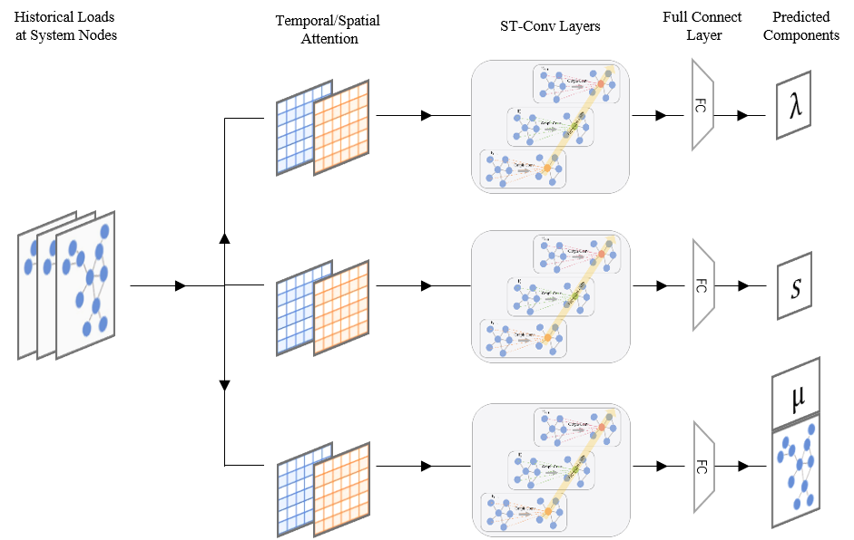
The proposed forecasting networks (GCN and its descendant: Attention-based Spatial-Temporal Graph Convolutional Network, ASTGCN) share the same structure of three similar branches (Fig.1), respectively forecasting different components . For each branch, the input is always the historical loads of nodes in a topological structure. Then it goes through a temporal/spatial attention layer and the loads’ value will be re-weighted according to their importance for prediction. After that, two identical consecutive layers of graph-temporal convolution would convolve nodes and their neighbours to get internal information. Finally, the full connect layer formulates the required shape of as output. Their composition produces the predicted LMP. In different branches, we set corresponding parameters as Tab.1 shows. The value of depends on which branch the layer is in. For , indicating an only value is determined for the energy component; for , indicating the possibility of congestion or not; for , using a 16-dimension tensor to represent characteristics of congestion. The detailed structure of ASTGCN will be introduced in the following sections.
[b] input dimension output dimension K1 T2 Attention layer ST-Conv 1 ST-Conv 2 Full connect
-
1
Graph receptive field
-
2
Temporal kernel’s shape
3 Model
The proposed forecasting model aims to solve this problem: Given , which denotes historical power loads of all the nodes in the power system, it needs to forecast LMP at all nodes for the same moment. We assumed that the power system contains nodes, and for each prediction, load data of previous Hours of loads are available.
A detailed zoom-in of one forecasting branch for instance is shown in Fig.2. Input load data comprising history loads at all nodes first come through a pre-trained attention block and thus become a mapped input. The attention block contains two masks respectively designed for time and space pattern extraction. After that, the mapped input will be processed by two consecutive ST-Conv blocks (made up of Graph and Temporal Convolution). Finally, a Fully Connect layer would synthesize the patterns learnt from the input and give an LMP prediction of all nodes for the next future moment.

3.1 Input
The initial input of the whole model contains the historical loads(MWh) at all nodes structured in table format. In the studied case, the previous hourly loads of hours are used as an input, whose shape is of .
3.2 Attention Block
The attention block consists of two masks corresponding to time and space dimension, namely spatial attention and temporal attention, to help adaptively identify the correlations between different time-points/system-nodes to reduce the computing power requirements of the original spatial-temporal graph convolution network. The masks are pre-trained with the train dataset, which is named "trainable mapping" in Fig.3. For example in node dimension, the history load input will be processed according to:
| (2) |
where , is the layer index, is node number, is time period length of the layer, , . , , are trainable parameters, and we use as an activation function. Attention masks are dynamically computed for different inputs, represents the correlation strength of node and node . A normalization is introduced to rows (Equ.3).
| (3) |
The internal procedure of the attention block is shown in Fig.3. The input historical nodal loads are consecutively re-weighted (can be regarded as a ’mapping’) first by temporalAtt and then spatialAtt mask based on their co-importance to forecasting LMP. More specifically, the input of the Attention Block will generate two attention masks ( for SpatialAtt Mask and for TemporalAtt Mask), and then the input would do dot-product with the two masks one after another to obtain a mapped input.

3.3 ST-Conv Block
To capture both patterns in time and space, a spatial-temporal convolutional (ST-Conv) block structure (ST-Conv block in Fig.2) is adopted in this model. It contains two modules: the first is a spectral graph convolution layer to extract the spatial features of LMP, then the second is a traditional convolution in the time dimension to exploit history dependencies for each node.
3.3.1 Graph Convolution
The spectral graph theory generalizes the convolution operation from grid-based data to graph structure data and accelerates it with spectral techniques. The power system is naturally one of such graphs. As for the graph, we applied ChebNetdefferrard2016convolutional to the graph convolution layer, which uses Chebyshev polynomial to reduce its computational costs and to accelerate the convolution process. The GCN layer based on ChebNet can be represented as follows:
| (4) |
where denotes the layer input, denotes the output. is the convolution kernel whose parameters rest with training and . represents a truncation of Chebyshev polynomial, and this also leads to a K-step receptive field of graph convolution. is a Chebyshev polynomial , where , .
| (5) |
where represents the output of the layer, denotes a standard convolution operation, is the trainable parameters of the temporal dimension convolution kernel, and the activation function is . Since the data along the temporal dimension are aligned (a.k.a. Euclidean), a standard convolution is enough to extract the potential influence from previous data.
3.4 Fully Connected Layer
The output of the ST-Conv block does not meet the shape that forecasting requires, so the output is altered to an appropriate shape with dot-product. As illustrated in Table. 1, the ST-Conv block output of shape is transposed to and then multiplied by a corresponding matrix to formulate the shape of . Finally, the three branches are respectively sum-reduced along with , which is of . The forecasting LMP of each node is a composition of all three branch outputs.
| (6) |
where , , and denote the output of the three branches, which are .
4 Training Method
All neural networks need training, details of how the training is set in the proposed model will be discussed in this section.
4.1 Loss Function
Loss function plays an important role in model training. The proposed model contains three branches, so the necessary part is to decide how each branch weighs in the overall loss function. We set varying loss functions for different branches as below:
| (7) | |||
| (8) | |||
| (9) |
where is 1-norm, is 2-norm. We set a target loss function weighing the ones above for the training process:
| (10) |
4.2 Parameter Initialization
The network contains a lot of parameters to be trained, or namely trainable parameters. They need to be pre-set before the training begins, which is called weight initialization. In deep learning networks, it could determine the layer outputs during the course of a forward pass through the network. If either the outputs’ vanishing or exploding occurs, loss gradients will either be too large or too small to flow backwards beneficially, and the network will take longer to converge, if it is even able to do so at all.
In the proposed network, Xavier Initialization glorot2010understanding is applied, which sets a layer’s weights to values chosen from a random uniform distribution that’s bounded between , where is the number of incoming network connections, or “fan-in” to the layer, and is the number of outgoing network connections from that layer, also known as the “fan-out”. According to Glorot and Bengio, Xavier Initialization can maintain the variance of activations and back-propagated gradients up or down the layers of a network and therefore brings substantially faster convergence.
4.3 Training Settings
The proposed LMP forecasting model is implemented with TensorFlow 1.14. The training process involves multiple hyperparameters. We tested the number of the terms of Chebyshev polynomial , and the accuracy is exalted with rising. However, the computing cost increased rapidly, so for a better trade-off in both forecasting performance and computing efficiency, we set Similarly, the kernel size of time-convolution is also set to . The model is optimized using Adam Optimizer and the initial learning rate is set to 1e-4 for 100 epochs.
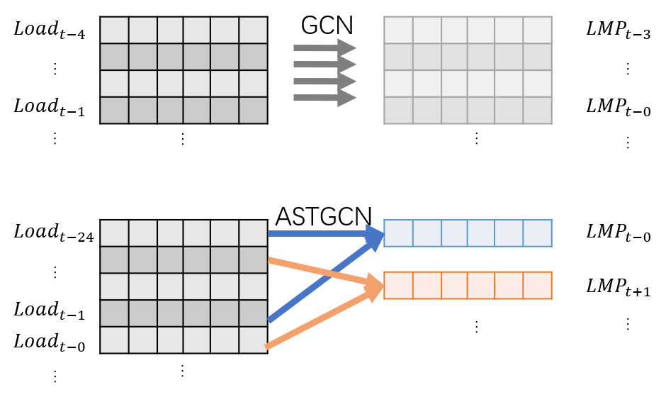
This work is examined by comparing MLP, GCN and ASTGCN. The following Fig. 4 shows how the outputs are generated with the corresponding inputs. The GCN only takes in the latest loads to give a forecast of LMP for the next period, while ASTGCN (adding temporal Conv and then attention) gives the forecast using previous hours.
5 Case Study
5.1 Dataset Description
The dataset involved in this work contains the topology of one IEEE-118 power system. The historical hourly loads and LMPs of all 118 nodes within 3 years are also included. It is divided into a train set and a test set with a proportion of 2:1. To be more specific, the first 2 years are set aside for training and the remaining 1 year is for testing.
| Topology | Vertices | Freq | Time Span |
| IEEE-118 | 118 | 1 point/hr | 3yr |
The dataset originates from the IEEE 118 case (of which the power line topology is given). We select real load data from the 2016-2018 PJM market pjm , including 26 load areas. The other 92 nodes’ loads are generated by linear-weighing the data above and adding noise as following:
For moment , denote the known load data by , then the generated load for the other 92 areas are:
| (11) |
where is a weight matrix obtained by sampling with Dirichlet distribution, which satisfies:
| (12) |
To induce system congestion, we add transmission capacity constraints to the highest mean-transmission-power lines. Also, we assume that bid curves are of quadratic function and are subject to stochastic noises. For generator at moment with active power output , the bidding function is:
| (13) |
where , are coefficients depending on time and noises:
| (14) | |||
| (15) |
where , are bidding coefficients of generator in IEEE 118, is standard normal distribution.
By solving the economic dispatch problem, we could acquire a dataset containing what is needed to train and evaluate the proposed model, which is separated into two parts: 2016-2017 as train dataset and 2018 as test dataset. In the case study, we suppose the model has acquired all history loads for each node as required in Fig. 4 and tries to forecast the upcoming LMP at each node in the power system.
With the generated dataset above, we compare the performance of load forecasting among traditional MLP (Multi-Layer Perceptron), GCN, and ASTGCN (GCN with temporal convolution and attention mechanism).
5.2 MLP v.s. GCN
The performance of GCN on the test dataset is shown in Table.3. To observe how GCN performs at a single node by time, we take the forecasted LMP curve at node 52 as an example in Fig.5.
| MAE/($/MWh) | RMSE/($/MWh) | MAPE/(%) |
| 0.6750 | 1.352 | 1.691 |

With focused sight into the red boxes on the LMP curve, we get detailed prediction performance visualizations in Fig.6 and Fig.7. It can be induced from the figures that GCN could make precise LMP forecasting, especially when the fluctuations are gentle like that in Fig.7.


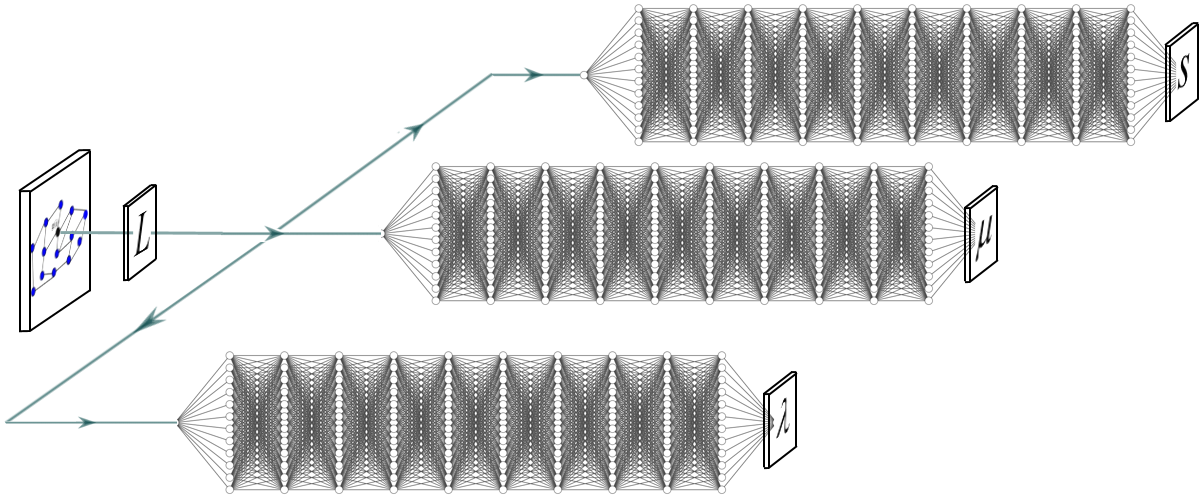
We then construct a Multi-Layer Perceptron (MLP) based model to represent what is widely adopted in prevailing LMP forecasting works for comparison. The disadvantage of MLP is that for each node a separate model needs to be constructed to forecast its LMP, and this also hampers MLP to find potential relations between different nodes. To compare fairly, a structure of MLP network resembling that of GCN with three branches is proposed as in Fig.8. The MLP uses 10 hidden layers with 128 neurons for each. We randomly select node 21, 49, 52 ,76 ,85, and 101 and train one MLP model for each nodes’ LMP forecasting. The comparison between MLP and GCN including MAE and RMSE is shown in Table.4 and Table.5, which strongly demonstrates GCN’s effectiveness as it achieves much lower errors in terms of both metrics.
| Node Index | GCN | MLP | Improve(%) |
| 21 | 1.024 | 4.480 | 81.38 |
| 49 | 1.251 | 2.706 | 74.48 |
| 52 | 1.071 | 3.150 | 77.12 |
| 76 | 1.111 | 1.211 | 55.01 |
| 85 | 1.016 | 1.176 | 53.34 |
| 101 | 1.061 | 2.021 | 70.13 |
| Node Index | GCN | MLP | Improve(%) |
| 21 | 1.427 | 7.910 | 81.88 |
| 49 | 1.750 | 5.130 | 75.87 |
| 52 | 1.623 | 6.777 | 79.40 |
| 76 | 1.597 | 2.004 | 43.16 |
| 85 | 1.508 | 1.934 | 43.64 |
| 101 | 1.570 | 3.874 | 69.72 |
According to the experiment, GCN shows a prominent advantage over the traditional MLP methods in LMP forecasting, including its great improvement in precision and simplification (as we need only one model for all nodes with GCN).
5.3 GCN v.s. ASTGCN
GCN could extract the topological correlations among nodes, but the history data of nodes’ loads are utterly omitted. However, in reality, previous loads’ trends usually have some impact on future LMP, on which basis traditional statistical models were built. Thus, an enhanced GCN with Temporal Convolution and Attention Mechanism taking historical data into account is proposed in this work.
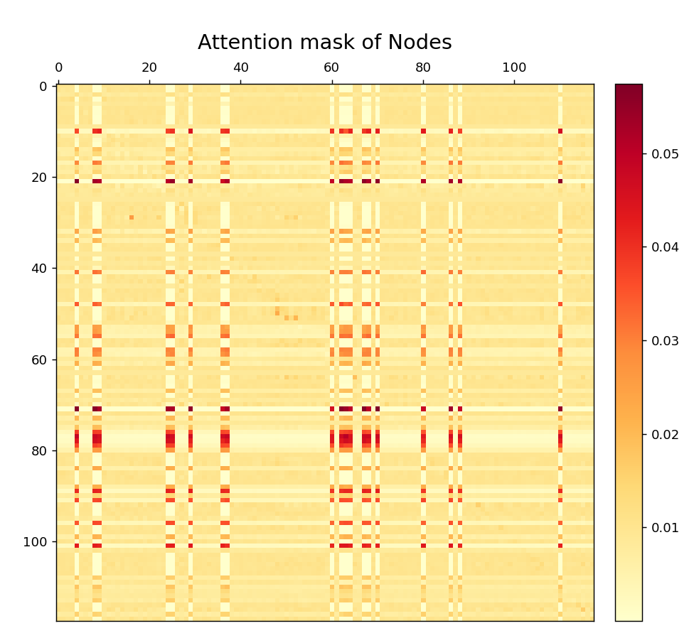
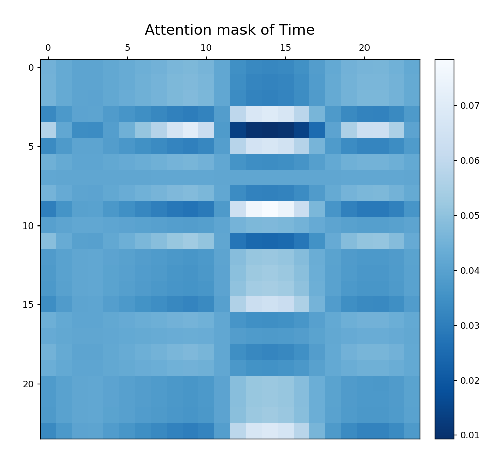
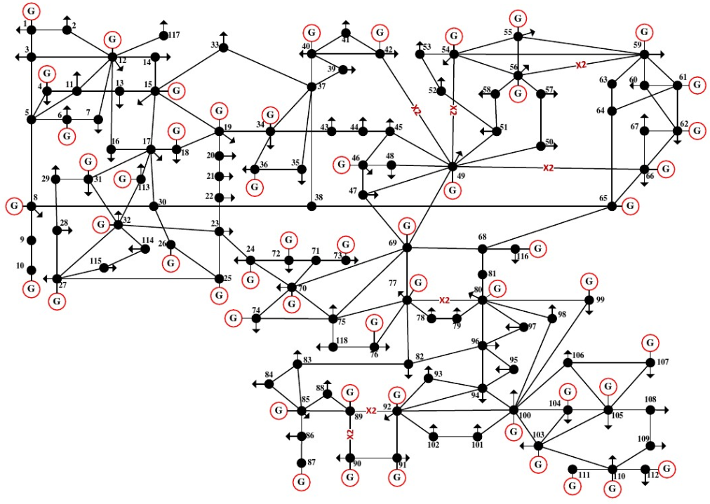
The introduced Graph Convolution takes effect in extracting topological information, while the added temporal convolution tries to discover the influence of time-continuity of power loads. In addition, the purpose of borrowing attention mechanism is to weigh historical node loads differently, meanwhile exalting the inter-weights of highly related nodes. Fig.9 shows a group of typical attention masks (illustrated in Section 3.2) among nodes generated with one input. The colored square of row column represents the influence of th node on th node (the redder means the higher importance). Thus, along the column axis, it is easy to discover some nodes are of higher influence on other nodes (like 5, 9, 10, 25, 26, 30, 37, 38, 61, 63, 64, 65, 68, 69, 71, 81, 87, 89, 111). From the topology of IEEE 118 (Fig. 11), most of these nodes are located in crossroads of power lines or at the only neighbour of generators. Some of them are not that special, while their high attention scores indicate their significance in LMP prediction. This feature shows an interpretable advantage of the proposed model highlighted hot nodes and connections’ strength among them. Fig.10 shows the attention scores among different periods in the same way.
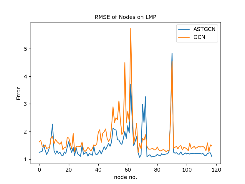
ASTGCN brings the model reduced RMSE at most nodes (shown in Fig. 12), showing a consistent superiority of ASTGCN in most cases. At nodes 70, 71 and 72, however, the ASTGCN fails to give a better prediction. This might comes from the accumulating errors when there occurs a highly fluctuating LMP curve. Since the ASTGCN additionally (compared with GCN) considers the historical loads, its tries to formulate a smooth temporal trend and this goes in the wrong direction for such cases and induces a bad RMSE at such nodes like node 71 (Fig. 13) with strong temporal fluctuations.


A comparison of performance is shown in Table.6. We can see generally a progressive advance in both MAE and RMSE is achieved via ASTGCN, while the accuracy of congestion factor remains almost the same.
| Model | Accuracy of congestion factor | MAE | RMSE |
| baseline GCN | 93.8242% | 0.987564 | 1.926941 |
| ASTGCN | 93.6758% | 0.822848 | 1.538259 |
In a nutshell, the attention could adaptively re-weigh the load according to their importance, and as well provide some interpretability of how we get some LMP prediction. Meanwhile, the temporal convolution puts enough emphasis on the previous load information which benefits the model by fusing traditional time series models.
6 Conclusion
To utilize both the system topology and time series of power loads in LMP forecasting, this paper proposes a novel LMP forecasting method based on the GCN. Several improvements are promoted, including the spatial-temporal convolution and attention mechanism. A three-branch network is introduced to predict the respective components of LMP. The case study shows that the proposed GCN-only model outperforms the existing MLP in both accuracy and simplicity by an average of 30% - 40% in prediction errors. With the ST-Conv blocks and attention blocks, ASTGCN succeeds to capture the dynamic spatial-temporal characteristics of LMPs. Further experiments on IEEE 118 dataset shows its capability to utilize more information and enhance precision.
Note that the GCN-based LMP forecating method can also be extended to similar applications that involve other time series related to system topological structure. Still, the proposed method reaches its bottleneck when it comes to frequent LMP spikes. This might comes from the inherence of convolution operations, and more efforts in network designing are expected to tackle such defects.
7 Acknowledgements
This work was supported by the National Key R&D Program of China under Grant No. 2020YFB0905900.
References
- [1] Griffin, J.M., Puller, S.L.: ‘Electricity deregulation: choices and challenges’. vol. 4. (University of Chicago Press, 2009)
- [2] Tan, Z., Ruan, G., Zhong, H., Xia, Q.: ‘Security pre-check method of bilateral trading adapted to independence of power exchange (in chinese)’, Automation of Electric Power Systems, 2018, 42, (10), pp. 106–113
- [3] Boucher, J., Smeers, Y.: ‘Alternative models of restructured electricity systems. Part 1: no market power’, Operations Research, 1999, 49, (6), pp. 821–838
- [4] Wang, J., Zhong, H., Yang, Z., Lai, X., Xia, Q., Kang, C.: ‘Incentive mechanism for clearing energy and reserve markets in multi-area power systems’, IEEE Transactions on Sustainable Energy, 2019, 11, (4), pp. 2470–2482
- [5] Chen, L., Wang, J., Wu, Z., Li, G., Zhou, M., Li, P., et al.: ‘Communication reliability-restricted energy sharing strategy in active distribution networks’, Applied Energy, 2021, 282, pp. 116238
- [6] Ruan, G., Zhong, H., Shan, B., Tan, X.: ‘Constructing demand-side bidding curves based on a decoupled full-cycle process’, IEEE Transactions on Smart Grid, 2020, 12, (1), pp. 502–511
- [7] Zhou, M., Wu, Z., Wang, J., Li, G.: ‘Forming dispatchable region of electric vehicle aggregation in microgrid bidding’, IEEE Transactions on Industrial Informatics, 2020, 17, (7), pp. 4755–4765
- [8] Fang, X., Li, F., Wei, Y., Cui, H.: ‘Strategic scheduling of energy storage for load serving entities in locational marginal pricing market’, IET Generation, Transmission & Distribution, 2016, 10, (5), pp. 1258–1267
- [9] Zhang, T., Wang, J., Zhong, H., Li, G., Zhou, M., Zhao, D.: ‘Soft open point planning in renewable-dominated distribution grids with building thermal storage’, CSEE Journal of Power and Energy Systems, 2020,
- [10] Veeramsetty, V., Chintham, V., Kumar, D.M.V.: ‘Probabilistic locational marginal price computation in radial distribution system based on active power loss reduction’, IET generation, transmission & distribution, 2020, 14, (12), pp. 2292–2302
- [11] Saebi, J., Taheri, H., Mohammadi, J., Nayer, S.S. ‘Demand bidding/buyback modeling and its impact on market clearing price’. In: 2010 IEEE International Energy Conference. (IEEE, 2010. pp. 791–796
- [12] Litvinov, E., Zheng, T., Rosenwald, G., Shamsollahi, P.: ‘Marginal loss modeling in LMP calculation’, IEEE transactions on Power Systems, 2004, 19, (2), pp. 880–888
- [13] Koopman, S.J., Ooms, M., Carnero, M.A.: ‘Periodic seasonal Reg-ARFIMA–GARCH models for daily electricity spot prices’, Journal of the American Statistical Association, 2007, 102, (477), pp. 16–27
- [14] Cuaresma, J.C., Hlouskova, J., Kossmeier, S., Obersteiner, M.: ‘Forecasting electricity spot-prices using linear univariate time-series models’, Applied Energy, 2004, 77, (1), pp. 87–106
- [15] Chitsaz, H., Zamani.Dehkordi, P., Zareipour, H., Parikh, P.P.: ‘Electricity price forecasting for operational scheduling of behind-the-meter storage systems’, IEEE Transactions on Smart Grid, 2017, 9, (6), pp. 6612–6622
- [16] Pircalabu, A., Benth, F.E.: ‘A regime-switching copula approach to modeling day-ahead prices in coupled electricity markets’, Energy Economics, 2017, 68, pp. 283–302
- [17] Ruan, G., Zhong, H., Wang, J., Xia, Q., Kang, C.: ‘Neural-network-based Lagrange multiplier selection for distributed demand response in smart grid’, Applied Energy, 2020, 264, pp. 114636
- [18] Zhou, M., Yan, Z., Ni, Y., Li, G., Nie, Y.: ‘Electricity price forecasting with confidence-interval estimation through an extended ARIMA approach’, IEE Proceedings-Generation, Transmission and Distribution, 2006, 153, (2), pp. 187–195
- [19] Contreras, J., Espinola, R., Nogales, F.J., Conejo, A.J.: ‘ARIMA models to predict next-day electricity prices’, IEEE transactions on power systems, 2003, 18, (3), pp. 1014–1020
- [20] Ruan, G., Zhong, H., Zhang, G., He, Y., Wang, X., Pu, T.: ‘Review of learning-assisted power system optimization’, CSEE Journal of Power and Energy Systems, 2020, 7, (2), pp. 221–231
- [21] Weron, R.: ‘Electricity price forecasting: A review of the state-of-the-art with a look into the future’, International journal of forecasting, 2014, 30, (4), pp. 1030–1081
- [22] Wu, W., Zhou, J., Mo, L., Zhu, C. ‘Forecasting electricity market price spikes based on Bayesian expert with support vector machines’. In: International Conference on Advanced Data Mining and Applications. (Springer, 2006. pp. 205–212
- [23] Fan, S., Mao, C., Chen, L.: ‘Next-day electricity-price forecasting using a hybrid network’, IET generation, transmission & distribution, 2007, 1, (1), pp. 176–182
- [24] Mandal, P., Haque, A.U., Meng, J., Martinez, R., Srivastava, A.K. ‘A hybrid intelligent algorithm for short-term energy price forecasting in the ontario market’. In: 2012 IEEE Power and Energy Society General Meeting. (IEEE, 2012. pp. 1–7
- [25] Mandal, P., Senjyu, T., Urasaki, N., Funabashi, T., Srivastava, A.K.: ‘A novel approach to forecast electricity price for PJM using neural network and similar days method’, IEEE Transactions on Power Systems, 2007, 22, (4), pp. 2058–2065
- [26] Lin, W.M., Gow, H.J., Tsai, M.T.: ‘Electricity price forecasting using enhanced probability neural network’, Energy Conversion and Management, 2010, 51, (12), pp. 2707–2714
- [27] Aggarwal, S.K., Saini, L.M., Kumar, A.: ‘Electricity price forecasting in deregulated markets: A review and evaluation’, International Journal of Electrical Power & Energy Systems, 2009, 31, (1), pp. 13–22
- [28] Rodriguez, C.P., Anders, G.J.: ‘Energy price forecasting in the Ontario competitive power system market’, IEEE transactions on power systems, 2004, 19, (1), pp. 366–374
- [29] Zhang, C., Li, R., Shi, H., Li, F.: ‘Deep learning for day-ahead electricity price forecasting’, IET Smart Grid, 2020, 3, (4), pp. 462–469
- [30] Lee, J.K., Park, J.B., Shin, J.R., Lee, K.Y. ‘A system marginal price forecasting based on an artificial neural network adapted with rough set theory’. In: IEEE Power Engineering Society General Meeting, 2005. (IEEE, 2005. pp. 528–533
- [31] Luo, S., Weng, Y.: ‘A two-stage supervised learning approach for electricity price forecasting by leveraging different data sources’, Applied energy, 2019, 242, pp. 1497–1512
- [32] Lin, W.M., Gow, H.J., Tsai, M.T.: ‘An enhanced radial basis function network for short-term electricity price forecasting’, Applied Energy, 2010, 87, (10), pp. 3226–3234
- [33] Mandal, P., Srivastava, A.K., Senjyu, T., Negnevitsky, M.: ‘A new recursive neural network algorithm to forecast electricity price for PJM day-ahead market’, International journal of energy research, 2010, 34, (6), pp. 507–522
- [34] Chang, Z., Zhang, Y., Chen, W.: ‘Electricity price prediction based on hybrid model of Adam optimized LSTM neural network and wavelet transform’, Energy, 2019, 187, pp. 115804
- [35] Lago, J., De.Ridder, F., De.Schutter, B.: ‘Forecasting spot electricity prices: Deep learning approaches and empirical comparison of traditional algorithms’, Applied Energy, 2018, 221, pp. 386–405
- [36] Zheng, K., Wang, Y., Liu, K., Chen, Q.: ‘Locational marginal price forecasting: A componential and ensemble approach’, IEEE Transactions on Smart Grid, 2020, 11, (5), pp. 4555–4564
- [37] Afrasiabi, M., Mohammadi, M., Rastegar, M., Kargarian, A.: ‘Probabilistic deep neural network price forecasting based on residential load and wind speed predictions’, IET Renewable Power Generation, 2019, 13, (11), pp. 1840–1848
- [38] Kipf, T.N., Welling, M.: ‘Semi-supervised classification with graph convolutional networks’, arXiv preprint arXiv:160902907, 2016,
- [39] Guo, S., Lin, Y., Feng, N., Song, C., Wan, H. ‘Attention based spatial-temporal graph convolutional networks for traffic flow forecasting’. In: Proceedings of the AAAI Conference on Artificial Intelligence. vol. 33. (, 2019. pp. 922–929
- [40] Wang, J., Shahidehpour, M., Li, Z.: ‘Security-constrained unit commitment with volatile wind power generation’, IEEE Transactions on Power Systems, 2008, 23, (3), pp. 1319–1327
- [41] Gaikwad, P.S. ‘Using Graph Convolutional Network and Message Passing Neural Networks for Solving Unit Commitment and Economic Dispatch in a Day Ahead Energy Trading Market Based on ERCOT Nodal Model’ [Professional]. The University of Texas at Arlington, 2020
- [42] Defferrard, M., Bresson, X., Vandergheynst, P. ‘Convolutional neural networks on graphs with fast localized spectral filtering’. In: Advances in neural information processing systems. (, 2016. pp. 3844–3852
- [43] Glorot, X., Bengio, Y. ‘Understanding the difficulty of training deep feedforward neural networks’. In: Proceedings of the thirteenth international conference on artificial intelligence and statistics. (JMLR Workshop and Conference Proceedings, 2010. pp. 249–256
- [44] PJM. ‘Historical metered load data’. (, 2019. Available from: https://dataminer2.pjm.com/feed/hrl_load_metered/definition