Tail of Distribution GAN (TailGAN): Generative- Adversarial-Network-Based Boundary Formation

Abstract

Generative Adversarial Networks (GAN) are a powerful methodology and can be used for unsupervised anomaly detection, where current techniques have limitations such as the accurate detection of anomalies near the tail of a distribution. GANs generally do not guarantee the existence of a probability density and are susceptible to mode collapse, while few GANs use likelihood to reduce mode collapse. In this paper, we create a GAN-based tail formation model for anomaly detection, the Tail of distribution GAN (TailGAN), to generate samples on the tail of the data distribution and detect anomalies near the support boundary. Using TailGAN, we leverage GANs for anomaly detection and use maximum entropy regularization. Using GANs that learn the probability of the underlying distribution has advantages in improving the anomaly detection methodology by allowing us to devise a generator for boundary samples, and use this model to characterize anomalies. TailGAN addresses supports with disjoint components and achieves competitive performance on images. We evaluate TailGAN for identifying Out-of-Distribution (OoD) data and its performance evaluated on MNIST, CIFAR-10, Baggage X-Ray, and OoD data shows competitiveness compared to methods from the literature.

I Introduction

Generative Adversarial Networks (GAN) can capture complex data with many applications in computer vision and have achieved state-of-the-art image synthesis performance. Recently, GANs have been used for anomaly detection which is critical in security, e.g. contraband detection. GANs succeed convergence in distribution metrics, but present limitations as they suffer from mode collapse, learn distributions of low support, and do not guarantee the existence of a probability density making generalization with likelihood impossible [1]. Unsupervised anomaly detection is examined since anomalies are not known in advance [2]. The normal class is learned and abnormal data are detected by deviating from this model.

Many anomaly detection methods perform well on low-dimensional problems; however, there is a lack of effective methods for high-dimensional spaces, e.g. images. Important tasks are reducing false negatives and false alarms, providing boundaries for inference of within-distribution and Out-of-Distribution (OoD), and detecting anomalies near low probability regions. Most papers use the leave-one-out evaluation methodology, $(K+1)$ classes, $K$ classes for normality, and the leave-out class for anomaly, chosen arbitrarily. This evaluation does not use the complement of the support of the distribution, and real-world anomalies are not confined to a finite set.

In this paper, we create a GAN-based model, the Tail of distribution GAN (TailGAN), to generate samples on the low probability regions of the normal data distribution and detect anomalies close to the support boundary. Using TailGAN, we leverage GANs for OoD sample detection and perform sample generation on the tail using a cost function that forces the samples to lie on the boundary while optimizing an entropy-regularized loss to stabilize training. The authors of this paper have recently proposed an invertible-residual-network-based generator, the Boundary of Distribution Support Generator (BDSG) [5], for anomaly detection using the IResNet and ResFlow models [6, 7]. In this paper, we include adversarial training and GANs to better generate samples on the low probability regions of the data distribution and detect anomalies near the support boundary. Our contribution is the creation of a GAN-based boundary formation model and we use GANs, such as Prescribed GAN (PresGAN) and FlowGAN [9, 10], that learn the probability of the underlying distribution and generate samples with high likelihoods. TailGAN improves the detection of anomalies and GANs that learn the probability density of the underlying distribution improve the anomaly detection methodology, allowing us to create a generator for boundary samples and use this to characterize anomalies.

II Related Work on Anomaly Detection

II-A GANs Using a Reconstruction-Based Anomaly Score

AnoGAN performs unsupervised learning to detect anomalies by learning the manifold of normal anatomical variability. During inference, it scores image patches indicating their fit into the learned distribution [11, 12]. In contrast to AnoGAN, Efficient GAN-Based Anomaly Detection (EGBAD) jointly learns an encoder and a generator to eliminate the procedure of computing the latent representation of a test sample [13]. Its anomaly score combines discriminator and reconstruction losses. GANomaly learns the generation of the data and the inference of the latent space, z. It uses an encoder-decoder-encoder in the generator and minimizing the distance between the vectors in z aids in learning the data distribution [14].

II-B GANs Performing Sample Generation on the Boundary

The GAN loss learns the mass of the distribution but to perform anomaly detection, we look at the boundary. The GAN optimization problem is given by $\text{argmin}_{\boldsymbol{\theta}_{g}}\text{dist}(p_{\textbf{x}}(\textbf{x}),p_{g}(\textbf{x}))$, where the distance metric, $\text{dist}(.,.)$, takes the specific form $\text{argmax}_{\boldsymbol{\theta}_{d}}\,f(D,p_{\textbf{x}}(\textbf{x}),p_{g}(\textbf{x}))$. For example, $\text{dist}(\textbf{x},\textbf{y})=||\textbf{x}-\textbf{y}||_{\infty}=\text{max}_{i}\,|x_{i}-y_{i}|$ and $\textbf{x},\textbf{y}\in\mathbb{R}^{d}$. The GAN loss is

$$\begin{split}\text{min}_{G}&\,\text{max}_{D}\operatorname{\mathbb{E}}_{\textbf{x}}[\text{log}(D(\textbf{x}))]+\operatorname{\mathbb{E}}_{\textbf{z}}[\text{log}(1-D(G(\textbf{z})))]\end{split}$$ (1)

where $\textbf{z}\sim p_{\textbf{z}}(\textbf{z})=N(\textbf{0},\textbf{I})$, $\textbf{x}\sim p_{\textbf{x}}(\textbf{x})$, and $G(\textbf{z})\sim p_{g}(\textbf{x})$. To generate samples on the distribution tail, MinLGAN uses minimum likelihood while FenceGAN changes (1). In contrast to the traditional GAN [17, 18], FenceGAN estimates the distance between $p_{g}(\textbf{x})$ and the tail of $p_{\textbf{x}}(\textbf{x})$. Its limitations are sampling complexity, the parallel estimation of $p_{\textbf{x}}(\textbf{x})$ and the tail of $p_{\textbf{x}}(\textbf{x})$, and disconnected boundary generation.

III The Proposed TailGAN

Section II.B has presented GANs for anomaly detection that perform sample generation on the support boundary of the normal data distribution. In this section, we present TailGAN for sample generation on the tail and anomaly detection.

III-A Boundary Generation: Improvement on Leave-One-Out

Before proceeding to explain TailGAN, it is important to first motivate the need to perform accurate sample generation on the tail. The leave-one-out evaluation, which can be restrictive for evaluating anomaly detection models, uses the disconnected components of the underlying multimodal distribution. For any annotated dataset with $K+1$ classes, the classification problem creates clusters and the decision criterion is a boundary for classification [20]. In high-dimensional spaces, classes form clusters and are disconnected components. Each cluster can have more than one modes. The disconnected components of the underlying distribution are usually known during the evaluation of the model while the modes of the distribution are not. Now, we denote a sample generated on the distribution’s tail by $T(\textbf{z})$, where $\textbf{z}\sim N(\textbf{0},\textbf{I})$ is the latent space, and using the $l_{p}$-norm, $||.||_{p}$, the clustering algorithm is given by

$$k(T(\textbf{z}))=\text{argmin}_{i=1,\dots,K}\,\text{dist}(T(\textbf{z}),\textbf{x}_{i})$$ (2)

$$\text{where }\text{dist}(T(\textbf{z}),\textbf{x}_{i})=\text{min}_{j=1,\dots,L}\,||T(\textbf{z})-\textbf{x}_{i,j}||_{p}$$ (3)

$$R(T(\textbf{z}),k)=\text{min}_{j=1,\dots,L}\,||T(\textbf{z})-\textbf{x}_{k,j}||_{p}$$ (4)

$$R(T(\textbf{z}),k)<\text{min}_{i\neq k,i=1,\dots,K}\,\text{min}_{j=1,\dots,L}\,||\textbf{x}_{i,j}-\textbf{x}_{k,j}||_{p}$$ (5)

where we use $K$ clusters from the leave-one-out methodology, $L$ samples from every class/cluster, and $\textbf{x}_{i,j}\in\mathbb{R}^{d}$ is the $j$-th sample of class $i$. With our boundary model, we can decide support membership to improve anomaly detection and also weight misses and false alarms. We can also generate anomalies, including adversarial anomalies, and the inequality presented in (5) states that the model’s generated samples are closer to the relevant class than any sample from any other class. Using (4) and (5), our boundary model improves the leave-one-out evaluation methodology by the margin given by $|R(T(\textbf{z}),k)-\text{min}_{i\neq k,i=1,\dots,K}\,\text{min}_{j=1,\dots,L}\,||\textbf{x}_{i,j}-\textbf{x}_{k,j}||_{p}|$.

III-B Framework for Sample Generation on the Tail

In this section, we develop our model, TailGAN, to detect anomalies near the low probability regions of the data distribution, i.e. strong anomalies. GANs generally do not guarantee the existence of a probability density and we use the recently developed PresGAN and FlowGAN models. We leverage such models for sample generation on the tail using two steps. The first step is to train either PresGAN or FlowGAN to learn the “normal” distribution, $G(\textbf{z})\sim p_{g}(\textbf{x})$. The random variable z follows a standard Gaussian distribution, $\textbf{z}\sim N(\textbf{0},\textbf{I})$, and the mapping from the latent space, z, to the data space, $\textbf{x}\in\mathbb{R}^{d}$, is given by $G(\textbf{z})$. The second step is to train a generator, $T(\textbf{z})$, to perform sample generation on the tail by minimizing

$$\begin{split}L_{tot}(\boldsymbol{\theta},\textbf{z},\textbf{x},G)=&\ w_{pr}\,L_{pr}(\boldsymbol{\theta},\textbf{z},G)+w_{d}\,L_{d}(\boldsymbol{\theta},\textbf{z},\textbf{x})\\ &+w_{e}\,L_{e}(\boldsymbol{\theta},\textbf{z},G)+w_{sc}\,L_{sc}(\boldsymbol{\theta},\textbf{z})\end{split}$$ (6)

where the total cost function, $L_{tot}$, comprises the probability cost, $L_{pr}$, the distance loss, $L_{d}$, the maximum-entropy cost, $L_{e}$, and the scattering loss, $L_{sc}$. The total cost in (6) comprises four terms. The probability cost penalizes probability density to find the tail of the data distribution while the distance loss penalizes large distance from normality using the distance from a point to a set. The maximum-entropy loss is for the dispersion of the samples [9, 1], and the scattering cost, $L_{sc}$, is defined by the ratio of the distances in the z and x spaces to address mode collapse. Hence, $L_{tot}$ in (6) is given by

$$\begin{split}&\ \frac{1}{N}\sum_{i=1}^{N}\left[w_{pr}\,p_{g}(T(\textbf{z}_{i};\boldsymbol{\theta}))+w_{d}\,\min_{j=1}^{M}||T(\textbf{z}_{i};\boldsymbol{\theta})-\textbf{x}_{j}||_{p}\right.\\ &\left.+\,w_{e}\,p_{g}(T(\textbf{z}_{i};\boldsymbol{\theta}))\log(p_{g}(T(\textbf{z}_{i};\boldsymbol{\theta})))\right.\\ &\left.+\,w_{sc}\,\frac{1}{N-1}\sum_{j=1,\,j\neq i}^{N}\dfrac{||\textbf{z}_{i}-\textbf{z}_{j}||_{p}^{q}}{||T(\textbf{z}_{i};\boldsymbol{\theta})-T(\textbf{z}_{j};\boldsymbol{\theta})||_{p}^{q}}\right]\end{split}$$ (7)

where we leverage the tradeoff between probability and distance in the first two terms of the loss, i.e. $L_{pr}$ and $L_{d}$, and where the model probability, $p_{g}(T(\textbf{z}_{i};\boldsymbol{\theta}))$, is given by

$$\,p_{\textbf{z}}(G^{-1}(T(\textbf{z}_{i};\boldsymbol{\theta})))\left|\text{det}\,\textbf{J}_{G}(T(\textbf{z}_{i};\boldsymbol{\theta}))\right|^{-1}$$ (8)

$$= \exp(\log(p_{\textbf{z}}(G^{-1}(T(\textbf{z}_{i};\boldsymbol{\theta}))))-\log(\left|\text{det}\,\textbf{J}_{G}(T(\textbf{z}_{i};\boldsymbol{\theta}))\right|))$$

where $\log(p_{\textbf{z}}(G^{-1}(T(\textbf{z}))))$ and $\log(\left|\text{det}\,\textbf{J}_{G}(T(\textbf{z}))\right|)$ are estimated by an invertible GAN model such as FlowGAN.

The parameters of the generator $T(\textbf{z})$, $\boldsymbol{\theta}$, are obtained by running Gradient Descent on $L_{tot}$, which can decrease to zero and is written in terms of the sample size, $M$, and the batch size, $N\leq M$. The distance term of the loss in (6), $L_{d}(\boldsymbol{\theta},\textbf{z},\textbf{x})$, depends on the training data, x. This distance term could use $G(\textbf{z})$ instead of x and in (7), our distance metric is defined using $M$ by $\text{dist}(T(\textbf{z}_{i}),\textbf{x})=\text{min}_{j=1,\dots,M}\,||T(\textbf{z}_{i})-\textbf{x}_{j}||_{p}$.

The loss in (7) uses the $l_{p}$-norm, $||.||_{p}$, and the scattering loss, $L_{sc}$, is based on the $l_{p}$-norm to power $q$, $||.||_{p}^{q}$, where $p$ and $q$ are real numbers and $p,q\geq 1$. In (7), the weight $w_{pr}$ is equal to $1$ and $w_{d}$, $w_{e}$, and $w_{sc}$ are hyperparameters. In (6)-(8), the gradient of $L_{tot}$ with respect to $T(\textbf{z})$ is well-defined and the change of variables formula in (8) has been used in a signal processing and nonlinear filtering algorithm in [22].

Figure 1: Generated samples of handwritten digits when we train PresGAN on MNIST using the PresGAN hyperparameter $\lambda=0.0002$, at $32$ epochs.

Figure 2: Probability of occurence of the generated images plotted against the disconnected component index using (2) and (3) when PresGAN is trained on MNIST using leave-one-out evaluation. The anomaly class is digit $2$.

MNIST	$L_{tot}$	$L_{d}$	$L_{sc}$
MNIST Digits 0-9	$4.73$	$471.96$	$0.82$
Fashion-MNIST	$14.91$	$1489.70$	$0.82$
KMNIST	$14.78$	$1476.81$	$0.82$

TABLE I: Evaluation of TailGAN comparing normality with anomaly cases using algorithm convergence criteria, total loss and distance loss. Anomaly cases: Fashion-MNIST, KMNIST.

Figure 3: Leave-one-out evaluation of TailGAN trained on MNIST using $L_{tot}$. The anomaly cases are the leave-out class and data from Fashion-MNIST.

Figure 4: Evaluation of TailGAN using AUROC on MNIST data.

Figure 5: Evaluation using AUPRC for anomaly detection on MNIST.

Figure 6: Generated samples when we train PresGAN on CIFAR-10 data.

IV Evaluation of TailGAN

We evaluate the TailGAN model using (i) algorithm convergence criteria such as the value of the objective cost function in (7) and the value of the distance cost, $L_{d}$, which is the distance from a point to a set and is based on the $l_{p}$-norm and the minimum operator, and (ii) the Area Under the Receiver Operating Characteristics Curve (AUROC) and the Area Under the Precision-Recall Curve (AUPRC). Experiments are performed on datasets of increasing complexity, MNIST, CIFAR, and Baggage X-Ray. In contrast to [2], we use the leave-one-out evaluation methodology and the detection of abnormal OoD data. The leave-one-out evaluation that uses the leave-out class as the anomaly leads to multimodal distributions with a support with disjoint components. The boundary of the support of the data distribution is defined using the threshold $\epsilon$.

TailGAN performs efficient sample generation on the tail of the distribution obviating the rarity sampling complexity problem, not requiring importance sampling [20]. For distributions with disconnected components, the TailGAN model achieves better performance than the convex hull extrema points.

IV-A Implementation of the Proposed TailGAN

We implement TailGAN in PyTorch and a vectorized implementation of the individual terms of the cost function in (7) has been created. We evaluate TailGAN using $p=q=2$ and because the choice of distance metric is important, $p=q=1$ or $p=2$ and $q=1$ could be used. We use $p_{g}(\textbf{x})$ from PresGAN which computes the entropy to address mode collapse. The first connection between TailGAN and our chosen base mode is $p_{g}(\textbf{x})$ while the second connection is model initialization, $\boldsymbol{\theta}_{t0}=\boldsymbol{\theta}_{g}$, where $\boldsymbol{\theta}_{t0}$ are the parameters of the generator $T(\textbf{z})$ at the start of training and $\boldsymbol{\theta}_{g}$ are the parameters of $G(\textbf{z})$.

Using $\boldsymbol{\theta}_{t0}=\boldsymbol{\theta}_{g}$, $T(\textbf{z})$ is trained to perform sample generation on the tail of the normal data distribution by starting from within the distribution, and this differs from the encoder-based initialization used in [2]. On the contrary, using random initialization for $\boldsymbol{\theta}$, $T(\textbf{z})$ is trained to perform sample generation on the tail by starting from outside the distribution. To compute the probability density, $p_{g}(\textbf{x})$, in (7) from the entropy which is estimated by PresGAN, we use the Lambert $W(.)$ function and Newton’s iterations. We evaluate TailGAN by first performing density estimation and then training $T(\textbf{z})$ using convolutional layers with batch normalization, minimizing (6) and (7).

IV-B Evaluation of TailGAN on MNIST Data

We first train PresGAN on MNIST until convergence using the leave-one-out methodology and the detection of abnormal OoD data. Next, we train TailGAN applying the objective cost function in (7). We examine different values for the batch size, $N$, and we use the entire training set for the sample size, $M$. We create $T(\textbf{z})$ using convolutional networks and we examine different architectures such as feed-forward and residual.

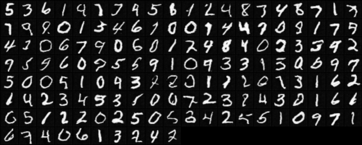
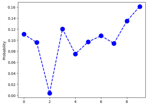
Figure 1 shows the generated samples at $32$ epochs when we train and use a modified version of PresGAN and the PresGAN hyperparameter $\lambda=0.0002$. As qualitative evaluation and visual measure, the MNIST canvas with the generated images in Fig. 1 shows that our chosen base model is trained to create realistic images of handwritten digits. All the digits from $0$ to $9$ are present in the canvas. Figure 2 depicts the probability of occurence of the generated images against the disconnected component index when PresGAN is trained on MNIST using the leave-one-out evaluation, when the anomaly class is digit $2$. The frequency of the generated data is computed using (2) and (3) based on the clustering algorithm in Sec. III.A.

We train TailGAN on MNIST until convergence and all the individual terms of the objective cost function, i.e. $L_{pr}$, $L_{d}$, $L_{e}$, and $L_{sc}$, decrease over epochs achieving convergence.

For the evaluation of TailGAN, Table I shows the algorithm convergence criteria in (6)-(8) produced by TailGAN trained on MNIST data. The values of the objective cost function, total loss, and distance loss, $L_{d}$, for abnormal OoD data are higher than the corresponding values for the normal data. The OoD anomalies are from Fashion-MNIST and KMNIST, and the total and distance losses are indicators of anomalies.

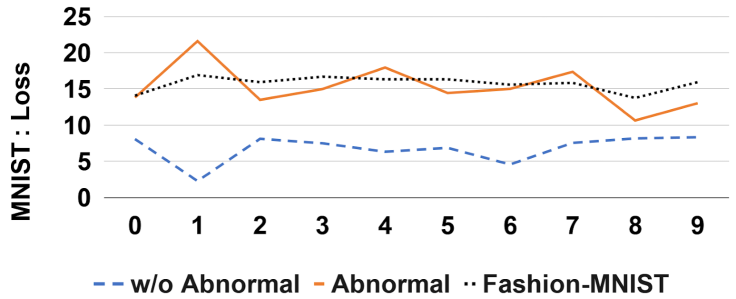
Using the leave-one-out evaluation on MNIST, we compute the cost function in (7), the total cost, the distance loss, and the scattering cost of $T(\textbf{z})$ of TailGAN. Figure 3 depicts the total loss, $L_{tot}$, for every MNIST digit for three different cases: (i) Without the abnormal digit, (ii) The abnormal digit, and (iii) Fashion-MNIST. The anomaly cases are the abnormal leave-out digit and Fashion-MNIST data. The algorithm convergence criteria, $L_{tot}$ and $L_{d}$, deviate from normality for the abnormal digits and the OoD cases as they are higher compared to the corresponding normal case values. Comparing TailGAN to the GANomaly and FenceGAN baselines trained on MNIST and evaluated on Fashion-MNIST, the $l_{2}$-norm distance loss in the x space is $3.1$, $1.7$, and $1.1$ times as much compared to the corresponding values for the normal case for TailGAN (i.e. Table I), GANomaly, and FenceGAN, respectively.

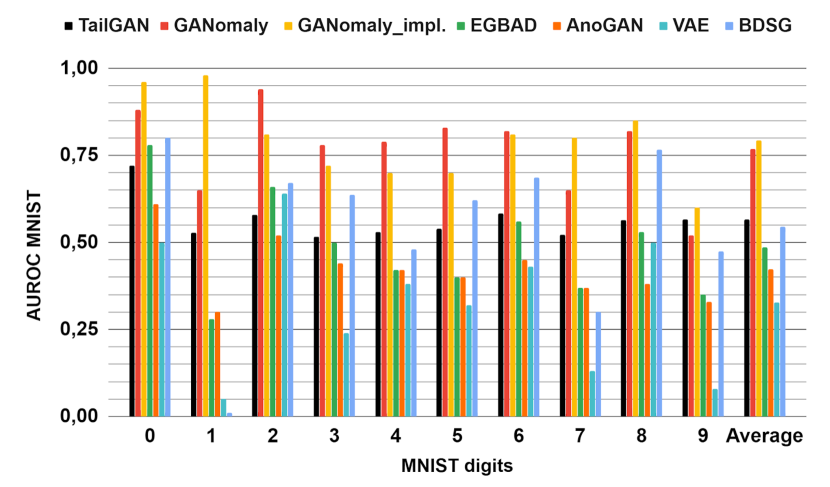
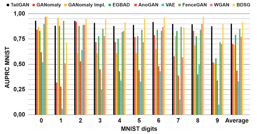
Figures 4 and 5 present the AUROC and AUPRC scores, respectively, for the evaluation of TailGAN on MNIST. During inference, we use the estimated probability density, the first term in (7) which addresses within or out of the distribution support, and the second term in (7) which computes $l_{p}$-norm distances for the anomaly score. Figures 4 and 5 examine the performance of TailGAN using the leave-one-out evaluation compared to several baselines, GANomaly, the implementation of GANomaly (GANomaly Impl.), EGBAD, AnoGAN, VAE, FenceGAN, and BDSG which has been proposed in [5].

CIFAR-10	$L_{tot}$	$L_{d}$	$L_{sc}$
CIFAR-10	$2.22$	$217.72$	$4.60$
CIFAR-100	$5.21$	$516.49$	$4.60$
SVHN	$7.76$	$771.02$	$4.60$
STL-10	$5.74$	$569.21$	$4.60$
CelebA	$6.31$	$626.26$	$4.60$
Baggage X-Ray	$51.67$	$5161.90$	$4.60$

TABLE II: Evaluation of TailGAN comparing normal with abnormal cases using algorithm convergence criteria, total loss and distance loss. Normality: CIFAR-10 classes 0-9. Anomaly cases: CIFAR-100, SVHN, STL-10, CelebA, Baggage X-Ray.

(a)

(b)

Figure 7: (a) Normal class image from the Baggage X-Ray dataset. (b) Anomaly class image from the Baggage X-Ray dataset containing knives and bottles.

Baggage X-Ray	$L_{tot}$	$L_{d}$	$L_{sc}$
Baggage X-Ray Normal	$3.21$	$319.22$	$2.83$
Baggage X-Ray Abnormal	$7.45$	$741.39$	$2.83$
CIFAR-10	$12.77$	$1274.32$	$2.83$
CIFAR-100	$13.14$	$1309.87$	$2.83$
SVHN	$9.87$	$983.72$	$2.83$
STL-10	$17.11$	$1706.81$	$2.83$

TABLE III: Evaluation of TailGAN on Baggage X-Ray data comparing normality with abnormal OoD cases using $L_{tot}$ from (7).

IV-C Evaluation of TailGAN on CIFAR-10 Data

To scale up the dimensions of the problem, we use the CIFAR-10 dataset and we hence go from $28\times 28$ dimensions of MNIST to $3\times 32\times 32$ dimensions of CIFAR. First, we train PresGAN for density estimation until convergence on CIFAR data and, then, we train TailGAN using convolutional neural networks with batch normalization. We train TailGAN using the entire training set for $M$ and our aim is to use TailGAN to accurately detect atypical, aberrant, abnormal samples.

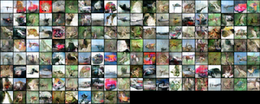
Figure 6 shows the generated samples when we use a modified version of PresGAN and the PresGAN hyperparameter $\lambda=0.0002$. As qualitative evaluation, the CIFAR-10 canvas with the generated images in Fig. 6 shows that our chosen base model is trained to create realistic images. All the classes are present in the canvas. Next, we train the proposed TailGAN by minimizing the cost function presented in (6)-(8). TailGAN achieves convergence on CIFAR-10 and $L_{pr}$, $L_{d}$, $L_{e}$, and $L_{sc}$ in (6) and (7) decrease over iterations, epochs, and time.

For model evaluation during inference, Table II compares the values of the loss terms for the normal class, CIFAR-10 data, with the corresponding values of the loss terms for the abnormal OoD data, CIFAR-100, SVHN, STL-10, CelebA, and Baggage X-Ray. In Table II, the distance loss is an indicator of anomalies and of the anomaly score, and both the total and distance losses are indicators of anomalies. The distance loss and the cost function values, $L_{d}$ and $L_{tot}$, are higher for the OoD data than the corresponding values for normality: $L_{tot}=2.22$ for normal data from CIFAR-10 and $L_{tot}=6.31$ for abnormal data from CelebA. Comparing TailGAN with the GANomaly and FenceGAN baselines trained on CIFAR-10 (Normal) and evaluated on CIFAR-100 (Abnormal), the $l_{2}$-norm distance loss in the x space is $2.3$, $1.1$, and $1.1$ times as much compared to the corresponding values for normality for TailGAN (i.e. Table II), GANomaly, and FenceGAN.

IV-D Evaluation of TailGAN on Baggage X-Ray Data

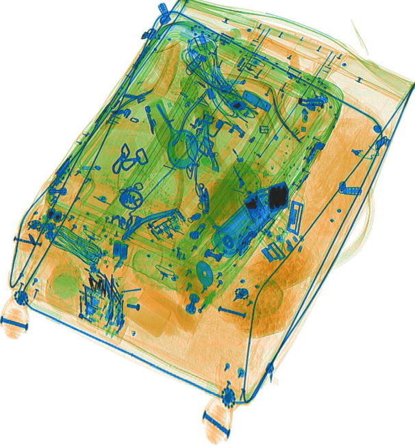
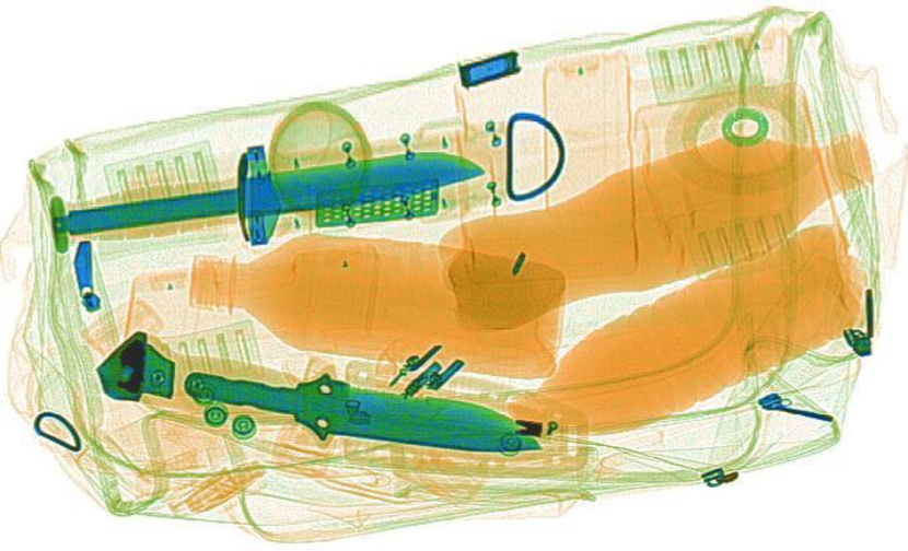
In this section, we evaluate TailGAN on Baggage X-Ray data. Figure 7 shows two example images, one from the normal class and one from the anomaly class, from the Baggage X-Ray dataset, where the abnormal image contains $2$ knives and $3$ bottles. Table III uses Baggage X-Ray data and compares the values of the losses for the normal class with the values of the losses for the abnormal OoD data. The distance loss and the cost function values, $L_{d}$ and $L_{tot}$, are higher for the Baggage X-Ray abnormal OoD data than the corresponding values for the normal Baggage X-Ray data, i.e. $L_{tot}=3.21$ for normal class data and $L_{tot}=7.45$ for abnormal OoD image data.

V Conclusion

In this paper, we have proposed the TailGAN model to perform anomaly detection and sample generation on the tail of the distribution of typical samples. The proposed TailGAN uses adversarial training and GANs, and minimizes the objective cost function in (6)-(8). Using GANs that can explicitly compute the probability density, we perform sample generation on the tail of the data distribution, we address multimodal distributions with disconnected-components supports, and we also address the mode collapse problem. The main evaluation outcomes on MNIST, CIFAR-10, Baggage X-Ray, and OoD data using the leave-one-out evaluation show that TailGAN achieves competitive anomaly detection performance.

VI Acknowledgment

This work was supported by the Engineering and Physical Sciences Research Council of the UK (EPSRC) Grant number EP/S000631/1 and the UK MOD University Defence Research Collaboration (UDRC) in Signal Processing.

References

- [1] E. Abbasnejad, J. Shi, A. van den Hengel, and L. Liu. A Generative Adversarial Density Estimator. In Proc. IEEE CVF Conference on Computer Vision and Pattern Recognition (CVPR), June 2019.
- [2] L. Ruff, R. Vandermeulen, N. Görnitz, L. Deecke, S. Siddiqui, A. Binder, E. Müller, and M. Kloft. Deep One-Class Classification. In Proc. 35th International Conference on Machine Learning, Stockholm, 2018.
- [3] L. Deecke, R. Vandermeulen, L. Ruff, S. Mandt, and M. Kloft. Image Anomaly Detection with Generative Adversarial Networks. In Machine Learning and Knowledge Discovery in Databases. ECML PKDD 2018. Lecture Notes in Computer Science, vol. 11051. Springer, 2019.
- [4] B. Schölkopf, J. Platt, J. Shawe-Taylor, A. Smola, and R. Williamson. Estimating the Support of a High-Dimensional Distribution. In Proc. Neural Computation, vol. 13, pp. 1443-1471, July 2001.
- [5] N. Dionelis, M. Yaghoobi, and S. A. Tsaftaris. Boundary of Distribution Support Generator (BDSG): Sample Generation on the Boundary. Paper Accepted for Publication in the Conference IEEE International Conference on Image Processing (ICIP), Oct. 2020.
- [6] J. Behrmann, W. Grathwohl, R. Chen, D. Duvenaud, and J. Jacobsen. Invertible Residual Networks. In Proc. 36th International Conference on Machine Learning (ICML), pp. 573-582, June 2019.
- [7] R. Chen, J. Behrmann, D. Duvenaud, and J. Jacobsen. Residual Flows for Invertible Generative Modeling. In Proc. Advances in Neural Information Processing Systems (NIPS), Dec. 2019.
- [8] K. He, X. Zhang, S. Ren, and J. Sun. Deep Residual Learning for Image Recognition. In Proc. IEEE Conference on Computer Vision and Pattern Recognition (CVPR), pp. 770-778, June 2016.
- [9] A. Dieng, F. Ruiz, D. Blei, and M. Titsias. Prescribed Generative Adversarial Networks. arXiv preprint, arXiv:1910.04302v1 [stat.ML], Oct. 2019.
- [10] A. Grover, M. Dhar, and S. Ermon. Flow-GAN: Combining Maximum Likelihood and Adversarial Learning in Generative Models. In Proc. Thirty-Second AAAI Conference on Artificial Intelligence, arXiv preprint, arXiv:1705.08868, Jan. 2018.
- [11] T. Schlegl, P. Seeböck, S. Waldstein, U. Schmidt-Erfurth, and G. Langs. Unsupervised Anomaly Detection with Generative Adversarial Networks to Guide Marker Discovery. In Proc. Information Processing in Medical Imaging (IPMI), Lecture Notes in Computer Science, vol. 10265. Springer, Cham, June 2017.
- [12] H. Zenati, C. Foo, B. Lecouat, G. Manek, and V. Ramaseshan Chandrasekhar. Efficient GAN-Based Anomaly Detection. Workshop track in the International Conference on Learning Representations (ICLR), Vancouver Canada, April 2018.
- [13] J. Donahue, P. Krähenbühl, and T. Darrell. Adversarial Feature Learning. In Proc. International Conference on Learning Representations (ICLR), April 2017.
- [14] S. Akçay, A. Atapour-Abarghouei, and T. Breckon. GANomaly: Semi-Supervised Anomaly Detection via Adversarial Training. arXiv preprint, arXiv:1805.06725v3 [cs.CV], Nov. 2018.
- [15] S. Akçay, A. Atapour-Abarghouei, and T. Breckon. Skip-GANomaly: Skip Connected and Adversarially Trained Encoder-Decoder Anomaly Detection. arXiv preprint, arXiv:1901.08954 [cs.CV], Jan. 2019.
- [16] I. Goodfellow, J. Pouget-Abadie, M. Mirza, B. Xu, D. Warde-Farley, S. Ozair, A. Courville, and Y. Bengio. Generative Adversarial Nets. In Proc. Advances in Neural Information Processing Systems (NIPS), pp. 2672-2680, Dec. 2014.
- [17] C. Wang, Y. Zhang, and C. Liu. Anomaly Detection via Minimum Likelihood Generative Adversarial Networks. In Proc. 24th International Conference on Pattern Recognition (ICPR), Aug. 2018.
- [18] C. Ngo, A. Winarto, C. Li, S. Park, F. Akram, and H. Lee. Fence GAN: Towards Better Anomaly Detection. In Proc. IEEE 31st International Conference on Tools with Artificial Intelligence (ICTAI), Portland, USA, Nov. 2019. DOI: 10.1109/ICTAI.2019.00028.
- [19] I. Haloui, J. Sen Gupta, and V. Feuillard. Anomaly detection with Wasserstein GAN. Preprint arXiv:1812.02463 [stat.ML], Dec. 2018.
- [20] R. Devon Hjelm, A. Paul Jacob, T. Che, A. Trischler, K. Cho, and Y. Bengio. Boundary-Seeking Generative Adversarial Networks. arXiv preprint arXiv:1702.08431v4 [stat.ML], Feb. 2018.
- [21] D. Hendrycks, M. Mazeika, and T. Dietterich. Deep Anomaly Detection with Outlier Exposure. In Proc. International Conference on Learning Representations (ICLR), May 2019.
- [22] N. Dionelis. Modulation-Domain Kalman Filtering for Single-Channel Speech Enhancement, Denoising and Dereverberation. Chapter 5: Phase-Sensitive Joint Noise Suppression and Dereverberation. PhD Thesis, Imperial College London, UK, Sept. 2019.
- [23] D. Hendrycks and K. Gimpel. A Baseline for Detecting Misclassified and Out-of-Distribution Examples in Neural Networks. In Proc. International Conference on Learning Representations (ICLR), 2017.