Regularising Inverse Problems with Generative Machine Learning Models

Abstract

Deep neural network approaches to inverse imaging problems have produced impressive results in the last few years. In this paper, we consider the use of generative models in a variational regularisation approach to inverse problems. The considered regularisers penalise images that are far from the range of a generative model that has learned to produce images similar to a training dataset. We name this family generative regularisers. The success of generative regularisers depends on the quality of the generative model and so we propose a set of desired criteria to assess generative models and guide future research. In our numerical experiments, we evaluate three common generative models, autoencoders, variational autoencoders and generative adversarial networks, against our desired criteria. We also test three different generative regularisers on the inverse problems of deblurring, deconvolution, and tomography. We show that restricting solutions of the inverse problem to lie exactly in the range of a generative model can give good results but that allowing small deviations from the range of the generator produces more consistent results.

Keywords: inverse problems, generative models, machine learning, imaging

1 Introduction

Solving an inverse problem is the process of calculating an unknown quantity, $x\in\mathcal{X}$, from observed, potentially noisy, measurements, $y\in\mathcal{Y}$. In this work $\mathcal{X}$ and $\mathcal{Y}$ are assumed to be real finite-dimensional vector spaces. The two are related by a forward model, $A:\mathcal{X}\rightarrow\mathcal{Y}$, that, for simplicity, is assumed to be linear, giving the equation

$$y=Ax.$$ (1)

Inverse problems are nearly always ill-posed: there does not exist a unique solution or small deviations in the data lead to large deviations in the solution. Addressing this is critical for applications where the solution is used to make decisions. Throughout this paper, we focus on image reconstruction problems, where $x\in\mathcal{X}$ is an image, but there are many other applications.

Generally, ill-posed problems are solved by incorporating some prior information; this is often given in the form of a regulariser in a variational regularisation framework [74, 42, 10]. Consider the optimisation problem

$$x^{*}\in\arg\min_{x}L_{y}(Ax)+\lambda R(x),$$ (2)

where $L_{y}:\mathcal{Y}\to[0,\infty]$ is a similarity measure; the constant $\lambda$ is a regularisation parameter and $R:\mathcal{X}\to[0,\infty]$ is a regulariser that is small when some desired property of the image is fulfilled. For example, Tikhonov regularisation encourages the reconstruction to be small in the 2-norm, while Total Variation (TV) regularisation [72] allows large gradients (e.g. edges) to occur only sparsely in the reconstruction. These hand-built regularisers are better suited to some types of images over others, e.g. TV is tailored to piece-wise smooth images. A natural question to ask is: given a set of images, which regulariser would work well? Alternatively, how can we produce regularisers that are tailored to specific data or tasks?

There is a wide body of research into learning regularisers. Approaches include using a regulariser to force reconstructions to be sparse in some learned basis for feasible images [3]. Others have included a network trained for denoising [83, 58, 70] or removing artefacts [54, 64, 28] in the regulariser term, favouring images that are unchanged by the network.  More recently, ‘adversarial regularisation’ [56] uses a neural network trained to discriminate between desired images and undesired images that contain artefacts. For a recent overview on approaches to using deep learning to solve inverse problems, see for example [7].

In this paper, we consider the case where the regulariser depends on a learned generative model. The assumption is that the plausible reconstructions exhibit local regularities, global symmetries or repeating patterns and so naturally lie on some lower dimensional manifold, a subset of $\mathcal{X}$. A generator $G:\mathcal{Z}\rightarrow\mathcal{X}$ takes points from a latent space, $\mathcal{Z}$, where ${\rm dim}(\mathcal{Z})\ll{\rm dim}(\mathcal{X})$, parameterising this lower dimensional manifold. In practice, the generator is taken to be a parameterised function, $G_{\theta}$, with parameters $\theta$, for example a neural network, trained such that the generated points $G_{\theta}(z)\in\mathcal{X}$ are similar to some pre-defined training set. In this work, we investigate regularisers [13, 25, 36, 80] that penalise values of $x\in\mathcal{X}$ that are far from the range of the generator, $G$, and call these generative regularisers. A popular example [13], revisited in Section 3.1.1, limits solutions to those that are exactly in the range of the generator,

$$x^{*}=G(z^{*}),\qquad z^{*}\in{\rm arg}\min_{z}\|AG(z)-y\|^{2}_{2}+\lambda\|z\|_{2}^{2}.$$ (3)

Generative regularisers combine the benefits of both a variational regularisation and data-driven approach. The variational approach builds on the advancements in model-based inverse problems over the last century, while the data-driven approach will provide more specific information than a hand crafted regulariser. The method remains flexible as the machine learning element is unsupervised and therefore independent of the forward model and the noise type. In this work, we test different generative regularisers, inspired by the literature, on deconvolution, compressed sensing and tomography inverse problems. The success of generative regularisers will depend on the quality of the generator. We propose a set of criteria that would be beneficial for a generative model destined for use in a inverse problems, and demonstrate possible methods of testing generative models against this criteria.

2 Generative Models

This section provides background on generators and generative models, focusing in particular on three approaches: Autoencoders, Variational Autoencoders and Generative Adversarial Networks.

2.1 Autoencoder (AE)

An AE has two parts, an encoder and a decoder. The encoder encodes an image in some latent space and the decoder takes a point in this latent space and decodes it, outputting an image. The lower dimensional latent space forces the network to learn representations of the input with a reduced dimensionality. Denote the encoder $E_{\psi}:\mathcal{X}\rightarrow\mathcal{Z}$ and the decoder $G_{\theta}:\mathcal{Z}\rightarrow\mathcal{X}$, neural networks with parameters $\psi$ and $\theta$. The networks are trained by minimising a reconstruction loss

$$\mathbb{E}_{x}\left\|x-G_{\theta}(_{\psi}(x))\right\|^{2}_{2}.$$ (4)

The expectation is taken empirically over the training dataset. Post training, the decoder can be used as a generator. With no structure imposed on the latent space, generating from random points in the latent space may not lead to outputs similar to the training set. Furthermore, points close in the latent space may not lead to similar generated images. Nevertheless, this method of training is simple and has recently been used in learned singular valued decomposition and for applications in sparse view CT [11, 63].

2.2 Probabilistic Models

In order to add greater structure and meaning to the latent space and to discourage unrealistic outputs from the generator we consider a probabilistic approach. Let $P^{*}$ be the probability distribution of desired solutions to the inverse problem. We consider a prior distribution, $P_{\mathcal{Z}}$, and push it through the generator, $G$, to give a generated distribution $P_{G}$ on $\mathcal{X}$. Sampling from the prior and then applying the generator allows samples to be taken from $P_{G}$. The generator, $G$, is chosen to minimise a distance between $P_{G}$ and $P^{*}$.

2.3 Generative Adversarial Network (GAN)

The choice of Wasserstein distance between $P_{G}$ and $P^{*}$ and an application of the Kantorovich-Rubinstein duality leads to the Wasserstein GAN [5], a popular generative model. Following the derivation given in [5, 33], the task of minimising the Wasserstein distance becomes

$$\min_{\theta}\max_{\psi}\ \mathbb{E}_{x\sim P^{*}}D_{\psi}(x)-\mathbb{E}_{z\sim P_{\mathcal{Z}}}D_{\psi}(G_{\theta}(z)).$$ (5)

The generator $G_{\theta}:\mathcal{Z}\rightarrow\mathcal{X}$ is as before, and we have introduced a discriminator $D_{\psi}:\mathcal{X}\rightarrow\mathbb{R}$ which must be 1-Lipschitz, enforced by an additional term added to (5)[33].

In the game theoretic interpretation of the GAN [29] a generative model competes with a discriminative model. The discriminator aims to accurately identify real images, maximising $\mathbb{E}_{x\sim P^{*}}D_{\psi}(x)$, from generated images, minimising $\mathbb{E}_{z\sim P_{\mathcal{Z}}}D_{\psi}(G_{\theta}(z))$. The generator tries to force the discriminator to label generated images as real, maximising $\mathbb{E}_{z\sim P_{\mathcal{Z}}}D_{\psi}(G_{\theta}(z))$.

For the numerical results in this paper we choose to use a Wasserstein GAN (5) as it is often more robust to a range of network designs and there is less evidence of mode collapse, when the generator learns just part of the target distribution, compared to the ‘vanilla’ GAN [5].

2.4 Variational Autoencoder (VAE)

For another choice of distance between $P_{G}$ and $P^{*}$, take the Kullback–Leibler (KL) divergence ($d_{\rm KL}(P^{*}\|P_{G})=\int_{\mathcal{X}}\log\frac{dP^{*}}{dP_{G}}dP^{*}$) which leads to the VAE [49]. Following the derivation in [49, 48], the VAE loss function can be written as

$$\mathbb{E}_{x\sim P^{*}}\left(\mathbb{E}_{z\sim\mathcal{N}_{x,\psi}}\left[\frac{\|x-G_{\theta}(z)\|_{2}^{2}}{2\rho^{2}}\right]+d_{KL}\left(\mathcal{N}_{x,\psi}\|P_{\mathcal{Z}}\right)\right)$$ (6)

where $\mathcal{N}_{x,\psi}:=\mathcal{N}(\mu_{\psi}({x}),{\rm diag}(\sigma^{2}_{\psi}({x})))$ and $\mu_{\psi},\sigma^{2}_{\psi}:\mathcal{X}\rightarrow\mathcal{Z}$ are the encoder mean and encoder variance, neural networks with parameters $\psi$. The constant $\rho$ is a hyperparameter chosen to reflect the ‘noise level’ in the training dataset.

We can interpret the two terms in (6) as a data fit and a regulariser term, respectively. In the first term, the reconstruction and the original image is compared. Encoding to a distribution, $\mathcal{N}_{x,\psi}$, enforces that points close to each other in the latent space should produce similar images. In the second term, the KL divergence encourages the encoded distributions to be close to the prior, $P_{\mathcal{Z}}$. The prior is usually taken to be the standard normal distribution. The balance between the two terms is determined by the noise level $\rho$.

2.5 Other Generative Models

Generative modelling is a fast growing field and there are other examples of generative models. Autoregressive models [23] generate individual pixels based on a probability distribution conditioned on previously generated pixels. Normalising flows and, more generally, invertible neural networks [43], map between a latent space and an image space of the same dimension and are designed to be bijective, with a tractable Jacobian. They can provide a generated distribution with tractable density. A recent invertible neural network example is a GLOW network [47] which has been used in regularisation of the form $R_{G}(x)=\|G^{-1}(x)\|_{2}^{2}$ [62]. Score based generative models, learn to approximate $\nabla p^{*}$, where $p^{*}$ is a probability density over the desired image distribution, $P^{*}$, and can then be used to sample from $P^{*}$ using Langevin dynamics [77]. They have also been used recently as priors for inverse problems, allowing the approximate posterior to be sampled using Monte Carlo methods [69, 45].

We will consider desired properties of generative models in more detail in Section 4.

3 Generative Regularisers for Inverse Problems

In this section, we bring together current approaches in the literature that penalise solutions of an inverse problem that are far from the range of the generator $G$. We consider variational regularisation (2) and regularisers of the form

$$R_{G}(x)=\min_{z\in\mathcal{Z}}F(G(z)-x)+R_{\mathcal{Z}}(z)$$ (7)

where $F:\mathcal{X}\rightarrow[0,\infty]$ and $R_{\mathcal{Z}}:\mathcal{Z}\rightarrow[0,\infty]$. We consider choices for $F$.

3.1 Choices of $F$ in (7)

3.1.1 Restricting solutions to the range of the generator

The characteristic function of an arbitrary set $\mathcal{C}$ is defined as

$$\iota_{\mathcal{C}}(t)=\cases{0&for $t\in\mathcal{C}$\\ \infty&for $t\notin\mathcal{C}$\\ }.$$

Taking $F(x)=\iota_{\{0\}}(x)$ and $R_{\mathcal{Z}}(z)=\|z\|_{2}^{2}$ in (7) gives (3) and describes searching over the latent space for the encoding that best fits the data. Their choice $R_{\mathcal{Z}}(z)$ reflects the Gaussian prior placed on the latent space. Bora et al. [13] first proposed this strategy, applying it to compressed sensing problems. There are a number of interesting applications using this method, such as denoising [80], semantic manipulation [32], seismic waveform inversion [60], light field reconstruction [19], blind deconvolution [8] and phase retrieval [38]. Bora et al. [13] assume the existence of an optimisation scheme that can minimise (3) with small error and from this probabilistically bound the reconstruction error. However, the non-convexity introduced by the generator makes any theoretical guarantees on the optimisation extremely difficult. Assuming the forward operator is a Gaussian matrix (the generator weights have independent and identically distributed Gaussian entries) and the layers of the generator are sufficiently expansive in size, there exists theoretical results on the success of gradient descent for optimising (3) [37, 53, 22].

This formulation can also be optimised by projected gradient descent [75, 44]:

$$w_{t+1}=x_{t}-\eta A^{T}(Ax_{t}-y)$$

$$z_{t+1}=\arg\min_{z}\|w_{t+1}-{G}(z)\|_{2}$$ (8)

$$x_{t+1}={G}(z_{t+1}).$$

With analogies to the restricted isometry property in compressed sensing [16], Shah and Hegde [75] introduce the Set Restricted Eigenvalue Condition (S-REC). If the S-REC holds, then the operator $A$ preserves the uniqueness of signals in the range of ${G}$. Theoretical work considers the case where $A$ is a random Gaussian matrix, and shows, under some assumptions, it satisfies the S-REC with high probability. In addition, if the generator is an untrained network, then the projected gradient descent approach with sufficiently small step size converges to $x^{*}$, where $Ax^{*}=y$ [75, 44, 68].

3.1.2 Relaxing the Constraints

Returning to Bora et al. [13], the authors note that as they increase the number of compressed sensing measurements, the quality of the reconstruction levels off rather than continuing to improve. They hypothesise that this occurs when the ground truth is not in the range of the generator. One could consider relaxing the constraint that the solution is in the range of the generator, for example setting $F(x)=||x||_{2}^{2}$ allows for small deviations from the range of the generator. One could also encourage the deviations to be sparse, for example by taking $F(x)=||x||_{1}$ [25, 39]. Some theoretical considerations for this softly constrained approach is given in [28]. This approach is similar to the approaches of [54, 64] where they take $G\circ E:\mathcal{X}\rightarrow\mathcal{X}$ an encoder–decoder network and define $R_{G}(x)=\|x-G(E(x))\|_{2}^{2}$. The idea is that this regulariser approximates the distance between $x$ and the ideal data manifold. Less explicitly, there are a number of approaches that extend the range of the original generator, through optimisation of intermediate layers of the network [59, 21, 34] or tweaking the generative model training in response to observed data [61, 41].

3.2 Additional regularisation

Additional regularisation on $\mathcal{Z}$ is given by $R_{\mathcal{Z}}$ in (7). The most common choice is $R_{\mathcal{Z}}(z)=\|z\|_{2}^{2}$ [13, 8] but there are other possibilities, for example $R_{\mathcal{Z}}(z)=\iota_{[-1,1]^{d}}(z)$ [80], where $d={\rm dim}\mathcal{Z}$. Often, the regularisation matches the prior on the latent space used in generator training. Menon et al. [59] discuss that $R_{\mathcal{Z}}(z)=\|z\|_{2}^{2}$ forces latent vectors towards the origin. However, most of the mass of the $d$-dimensional standard normal prior on their latent space is located near the surface of a sphere of radius $d$. Instead, they use a uniform prior on $d\mathcal{S}^{{d}-1}$. This idea has also been explored for interpolations in the latent space [84]. In addition, the prior on the latent space may not be a good model for the post-training subset of $z$ that maps to feasible images. For a VAE there may be areas of the latent space that the generator has not seen in training and for a GAN, there could be mode collapse. A few recent papers consider how to find the post training latent space distribution [20, 9].

Other regularisation choices could be based on features of the image, $x={G}(z)$. For example VanVeen et al. [82] use $R_{\mathcal{Z}}(z)={\rm TV}({G}(z))$. For a GAN generator, it is possible to take the regularisation term to be the same as the generator loss $R_{\mathcal{Z}}(z)=\log(1-D(G(z)))$. This regulariser utilises the discriminator, ${D}$, which has been trained to differentiate generated from real data. Examples include inpainting [86, 51] and reconstruction from an unknown forward model [4].

3.3 Other Approaches

There are a number of ideas that are linked to earlier discussions in this Section but we will not cover in detail. A major benefit of (2) is the flexibility to changes in the forward model. We have threfore ignored conditional generative models [1, 66, 85, 57, 88, 65, 76] and those that train with a specific forward model in mind [54, 46, 35]. We also exclude work that uses an untrained neural network, for example Deep Image Priors [82, 81, 26] or [36].

4 Generative Model Evaluation

Typically the aim of a generator has been to produce high fidelity images. However, the success of (7) relies not just on the ability of the generator to produce a few good images but to be able to produce every possible feasible image. In this section, we discuss desired properties for a generator trained for use in inverse problems and numerically explore methods to test these properties.

4.1 Desired Properties

To evaluate a generative model, in the context of inverse problems, we consider two overall aims which we will go on to further decompose:

A

Samples from the generator are similar to those from the target distribution.

B

Given a forward model and an observation, the image in the range of the generator that best fits the observation can be recovered using descent methods.

We split aim A into a set of properties:

A1

The generator should be able to produce every possible image in the target distribution. That is, for all $x\in\mathcal{X}$ such that $x$ is similar to images in the training dataset, there exists $z\in\mathcal{Z}$ such that $G(z)=x$.

A2

The generator should not be able to produce images far from the target distribution. That is, for all $x\in\mathcal{X}$ such that $x$ is not similar to images in the training dataset, then there does not exist $z\in\mathcal{Z}$ such that $G(z)=x$.

A1 includes that the generator should be robust to mode collapse and that the model should not trivially over-fit to the training data.

In the probabilistic case, with a prior over the latent space, Property A becomes:

A

That samples from the latent space, when mapped through the generator, will produce samples that approximate a target distribution. We should have that $d(P^{*},P_{G})$ is small for some distance measure $d$.

We also note that in the probabilistic case, A1 and A2 are not independent. By assigning probability mass to parts of the image space close to the target distribution, it is less likely that images far from the target distribution can be generated. In the probabilistic case, a third Property is added:

A3

The generator should map high probability vectors in the latent space distribution to high probability images in the target distribution.

It is possible that A1 and A2 are satisfied but not A3. Note that these properties may not be possible to achieve for a given dataset.

We define two properties for Property B, these are

B1

The generator should be smooth with respect to the latent space, $\mathcal{Z}$.

B2

The area of the latent space, $\mathcal{Z}$, that corresponds to images similar to those in the training set should be known.

B1 ensures that gradient–based optimisation methods can be used. Continuity is also desirable: we wish that, in some way, points close in the latent space should produce similar images. B2 considers that we need to have a distribution on or subset of $\mathcal{Z}$ to sample from in order to use the generator to sample images. This distribution may not necessarily be equal to any priors on the latent space used during training. We recognise that B1 and B2 are perhaps vague, and are potentially not sufficient for Property B. It is an area for future work to consider making these statements precise enough to support theoretical work.

4.2 Generative Model Evaluation Methods

There are a wide range of existing generative model evaluation methods [14], focused mostly on Property A. We assume the availability of some test data drawn from the same distribution as the training data and unseen by the generative model. The average log likelihood [29] of test data under the generated distribution is a natural objective to maximise. There is evidence, however, that the likelihood is generally unrelated to image quality and is difficult to approximate in higher dimensions [78]. To calculate a distance between generated and desired distributions, one possibility is the earth movers distance (EMD) [71], a discretised version of the Wasserstein distance. One could also encode the generated and unseen data in a lower dimensional space before taking distance calculations, for example by taking the outputs of one layer of any neural network trained for classification [40, 31]. A model that overfits to the training data would perform perfectly in these distance measures. Also, the low dimensional representation used for the evaluation is likely to have the same inherent problems and drawbacks as the embedding learnt by the generative model. Similarly, a number of tests train an additional, separate, neural network discriminator to distinguish between test data and generated data [5, 55]. Failure to classify the two is a success of the generative model. For testing a GAN, the new discriminator is unlikely to be able to pick up failures that the original discriminator, used in training, missed. Finally, Arora et al. [6] estimate the size of the support of the generated distribution. A low support size would suggest mode collapse. Their technique depends on manually finding duplicate generated images which can be time consuming and require expert knowledge.

Property B is less explored in the literature. One approach is to directly attempt to reconstruct test data by finding a latent space vector that when pushed through the generator, matches the data. With these found latent vectors, analysing their locations could check Property B2. To test the smoothness of the generator with respect to the latent space, Property B1, many previous papers, including the original GAN and VAE papers [29, 49], interpolate through the latent space, checking for smooth transitions in the generated images.

4.3 Numerical Experiments

In this Section, we evaluate AE, VAE and GAN models against the desired properties given in Section 4.1. We consider experiments on two datasets. Firstly, a custom made Shapes dataset with 60,000 training and 10,000 test $56\times 56$ grey-scale images. Each image consists of a black background with a grey circle and rectangle of constant colour. The radius of the circle; height and width of the rectangle; and locations of the two shapes, are sampled uniformly with ranges chosen such that the shapes do not overlap. This dataset is similar to the one used in [66]. Secondly, the MNIST dataset [52] consists of $28\times 28$ grey-scale images of handwritten digits with a training set of 60,000 samples, and a test set of 10,000 samples. For examples of both datasets, see the ground truth images in Figure 2.

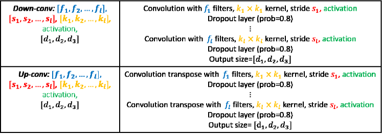
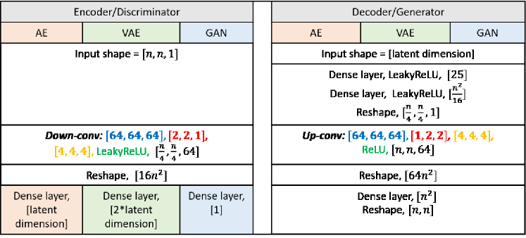
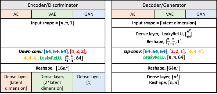
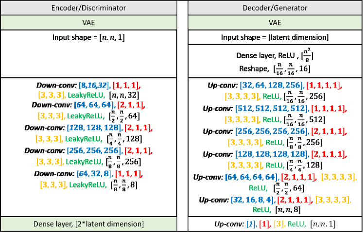
Architecture details are given in the appendix. We chose to use the same generator network for all three models, for comparison. Architecture choices were guided by [49, 33, 73]. All models have gone through a similar amount of optimisation of hyperparameters, including: the noise level $\rho$ in the VAE decoder (6); the latent dimension; number of layers; choice of convolution kernel size; drop out probability; leaky ReLU coefficient and learning rate. In order to select hyperparameters we manually inspected generated images. Models were built and trained using Tensorflow [30] in Python and made use of the Balena High Performance Computing Service at the University of Bath. The models were trained using a single Dell PowerEdge C8220X node, with two Intel E5-2650 v2 CPU, 64 GB DDR3-1866 MHz Memory and an Nvidia K20X GPU, 6 GB memory. The MNIST and Shapes VAE models taking approximately 25 and 45 minutes to train, respectively.

4.3.1 Reconstructing a Test Dataset

Property A1 asks that the generator is able to produce every image in the target distribution. Gradient descent with backtracking line search (Algorithm 1, in the appendix) is used to approximate

$$z^{*}(x)\in\arg\min_{z}\|G(z)-x\|_{2}^{2},$$ (9)

for each $x\in\mathcal{X}_{{\rm test}}$, an unseen test dataset. For the AE and VAE, the algorithm is initialised at the (mean) encoding of the test image, $E_{\psi}(x)$ and $\mu_{\psi}(x)$, respectively. For the GAN, we take 4 different initialisations, drawn from a standard normal distribution, and take the best result. We find empirically, especially for the GAN, that different initialisations lead to different solutions.

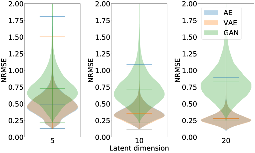
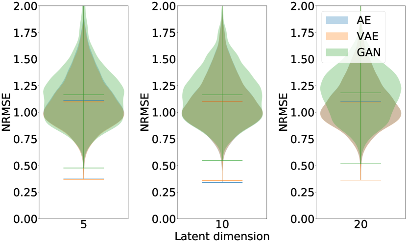
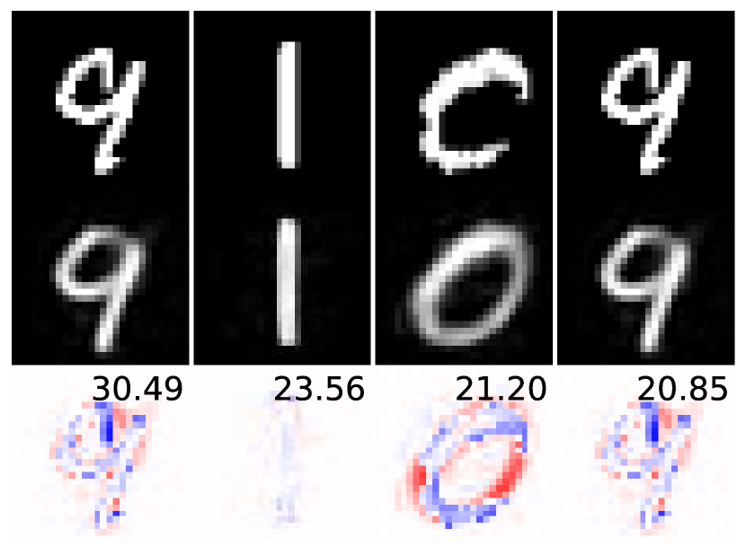
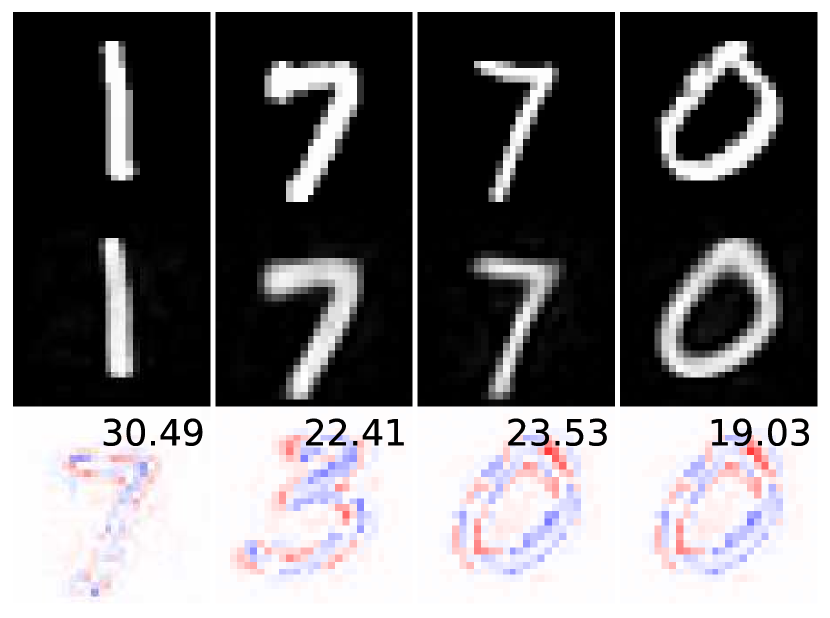
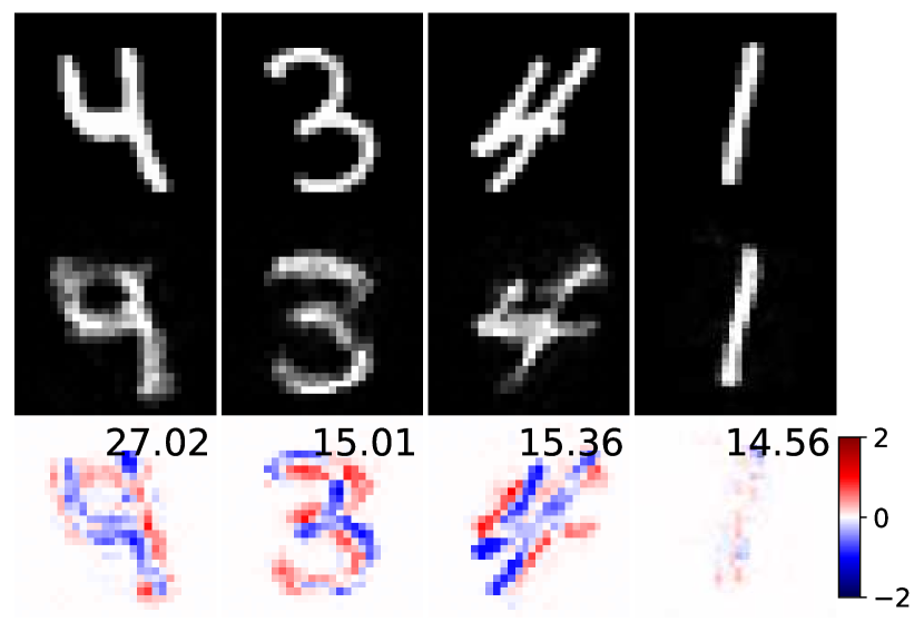
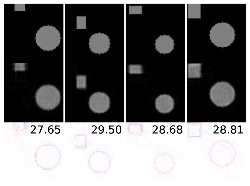
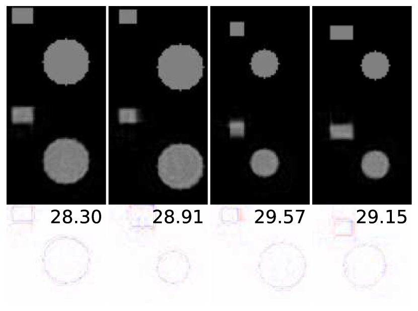
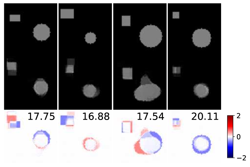
Figure 2 shows $\|G(z^{*}(x))-x\|_{2}/\|x\|_{2}$, the normalised root mean squared error (NRMSE) for reconstructions on Shapes and MNIST for the three different generator models. We see that, for both datasets, the AE and VAE have almost identical reconstruction results and the GAN results are comparatively worse. For the Shapes dataset the difference in results between the three generative models is less stark. In addition, NRMSE values are given for three different latent dimensions to show that the results are not sensitive to small changes in latent dimension. Latent dimensions of 8 and 10 for MNIST and Shapes, respectively, are used in the rest of this paper. Figure 2 also shows reconstruction examples providing context to the results in Figure 2. Numerical values on the image use the Peak-Signal-to-Noise-Ratio (PSNR, see definition 3.5 in [15]). The non-circular objects in the GAN results for Shapes could be a failure of the discriminator to detect circles.

(a) MNIST dataset

(b) Shapes dataset

Figure 1: NRMSE between values of $G\left(\arg\min_{z}\|G(z)-x\|_{2}\right)$ and $x$ and plotted as a histogram for all $x\in\mathcal{X}_{\rm test}$. The horizontal lines show the median and range and the shaded area a histogram. Note the brown colour is the result of the overlapping orange (VAE) and blue (AE).

(c) AE – MNIST

(d) VAE – MNIST

(e) GAN – MNIST

(f) AE – Shapes

(g) VAE – Shapes

(h) GAN – Shapes

Figure 2: Example reconstructions for the MNIST and Shapes dataset with eight ten-dimensional generative models respectively. In each sub-figure, the top row shows the ground truth, second row the reconstruction and third row the difference between the two.

4.3.2 Distance Between $P_{G}$ and $P^{*}$

(a) MNIST

(b) Shapes

Figure 3: EMD between the test dataset and samples from a trained generator.

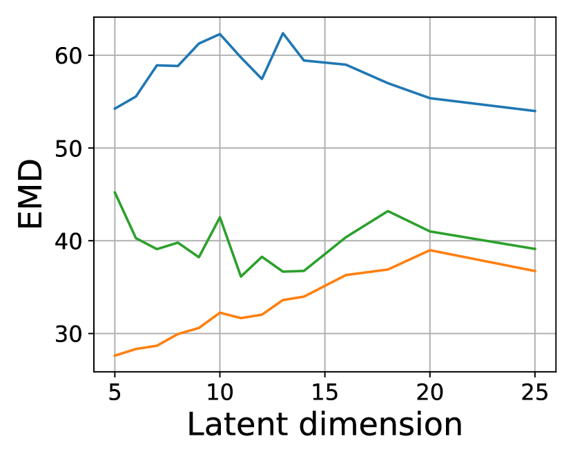
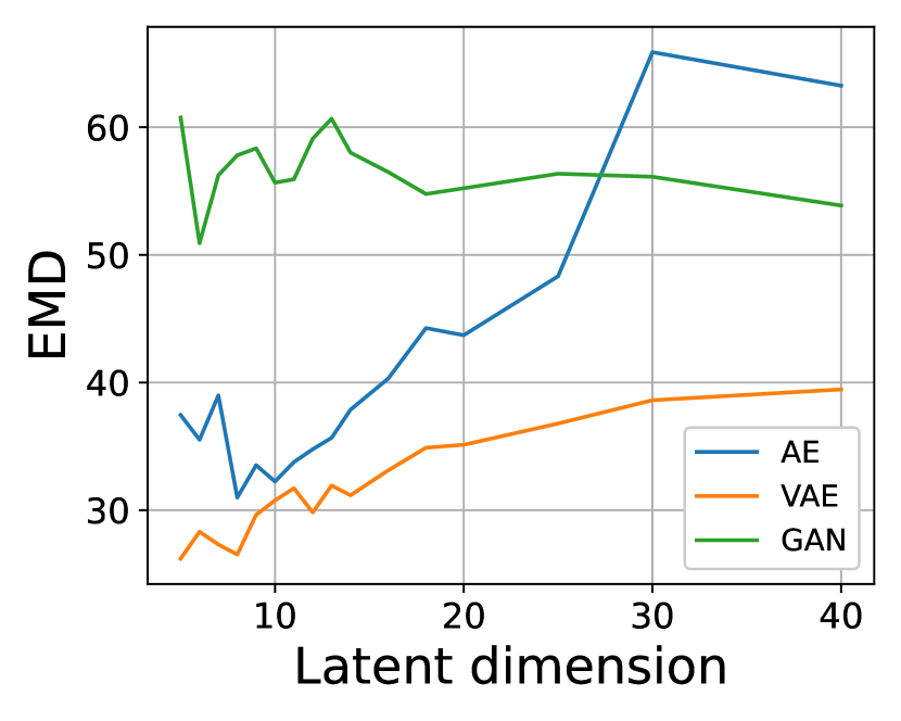
To investigate Property A3, the EMD [71] is calculated between empirical observations of the generated and the data distributions $P_{G}$ and $P^{*}$. For the sets of test and generated images, $\mathcal{X}_{{\rm test}}=\{x_{1},\ldots,x_{N}\}$ and $\{G(z_{1}),\ldots,G(z_{N}):z_{i}\sim\mathcal{N}(0,I)\}$, the EMD between their empirical distributions is defined as

$$\min_{f}\left\{\sum_{i,j=1}^{N}f_{i,j}\|x_{i}-G(z_{j})\|^{2}_{2}:0\leq f_{i,j}\leq 1,\sum_{i=1}^{N}f_{i,j}=1,\sum_{j=1}^{N}f_{i,j}=1\right\}.$$ (10)

The EMD is calculated using the Python Optimal Transport Library [27] with $N=10,000$, the full test set. The results are given in Figure 3. In both the MNIST and Shapes examples, the VAE has a lower EMD across the latent dimensions. The AE is added to this plot for comparison purposes but, as there is no prior on the latent space, $z_{i}\sim\mathcal{N}(0,I)$ may not be a suitable choice to sample from.

4.3.3 Visualisations of the Latent Space

(a) MNIST

(b) Shapes

Figure 4: Comparisons of the latent space encodings of a test dataset with a standard normal distribution by projecting the vectors into 2 dimensions. Encodings of the test dataset are in orange and the standard normal vectors in blue.

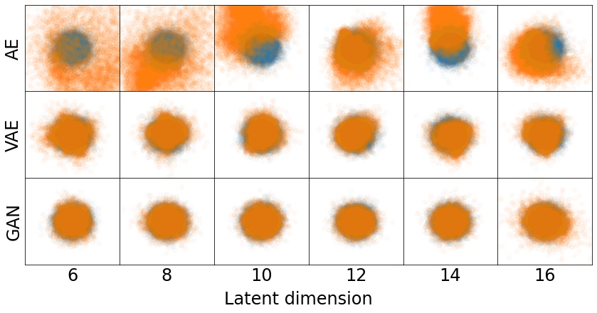
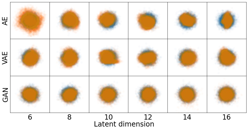
Property B2 requires that the area of the latent space that maps to feasible images is known. There is no prior on the latent space enforced for AEs and a $\mathcal{N}(0,I)$ prior is imposed for VAEs and GANs. In Figure 4, gradient descent with backtracking (Algorithm 1 in the appendix) is used to approximate (9), finding a latent vector $z^{*}(x)$ for each $x\in\mathcal{X}_{{\rm test}}$. For comparison, the values $z^{*}(x)$ for the test set and 10,000 vectors drawn from a standard normal distribution are randomly projected into 2 dimensions. The encodings in the latent space match the prior $\mathcal{N}(0,I)$ for VAEs and GANs. For AEs, there are examples in lower latent dimensions, where the area covered by the encodings does not match a standard normal distribution.

4.3.4 Generating Far from the Latent Distribution

(a) MNIST

(b) Shapes

Figure 5: Images generated far from the high-probability region of the prior distribution.

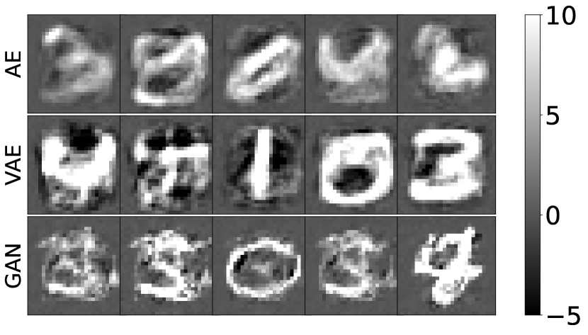
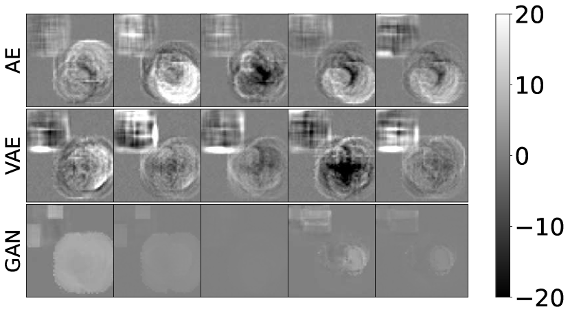
A known latent space gives known areas to sample from to produce new images. Figure 5 shows image examples generated far from a standard normal distribution. The images are not recognisable as similar to the training datasets. This emphasises the importance of Property B2, that the area of the latent space that corresponds to images similar to those in the training set should be known.

4.3.5 Interpolations in the Latent Space

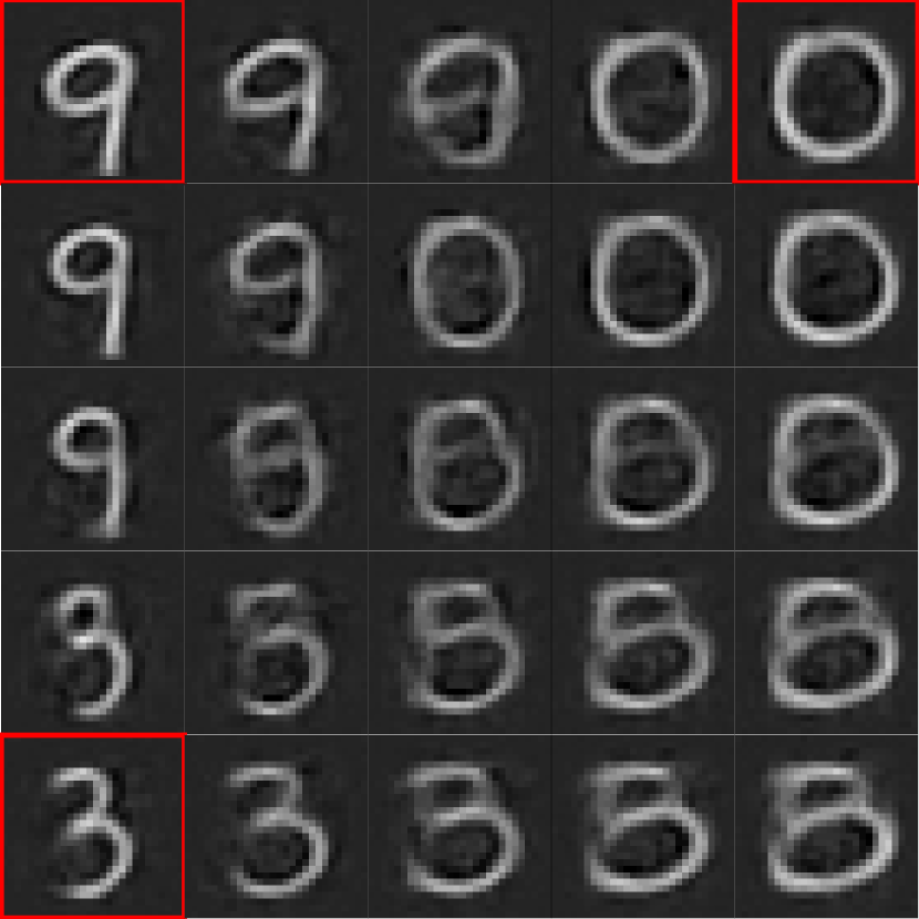
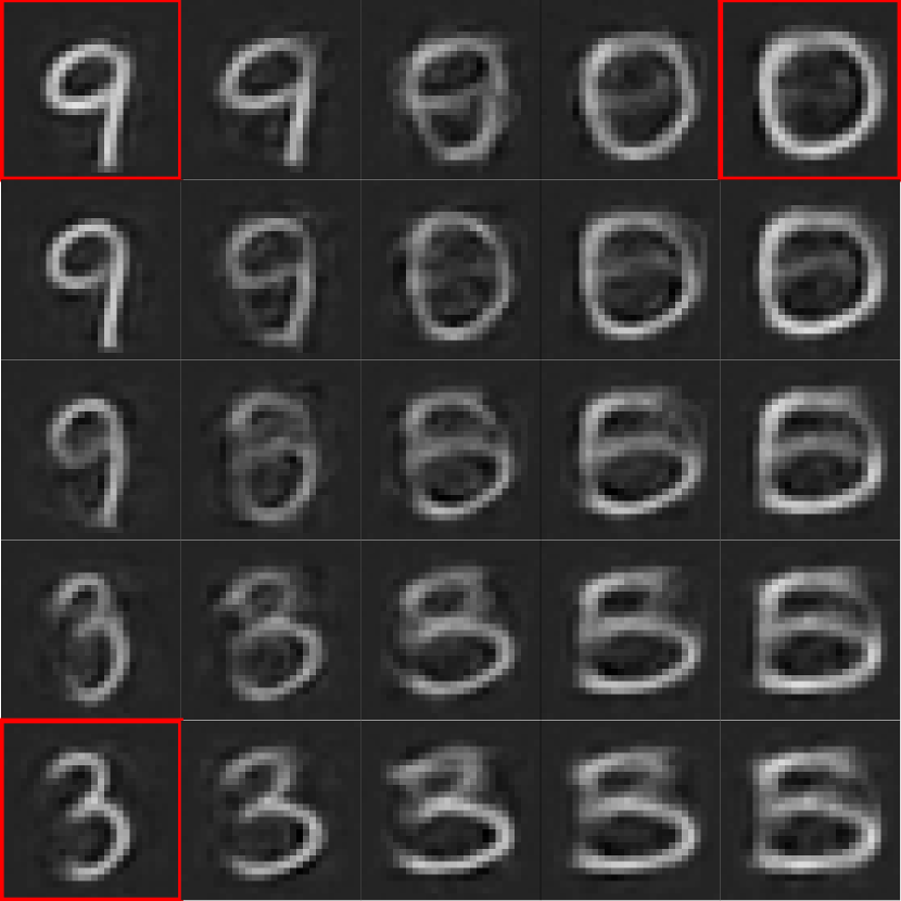
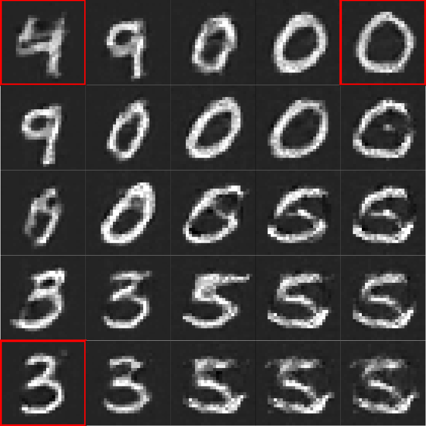
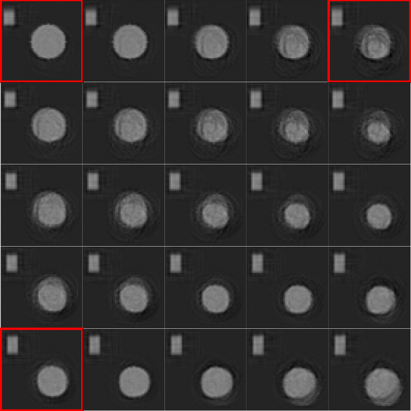
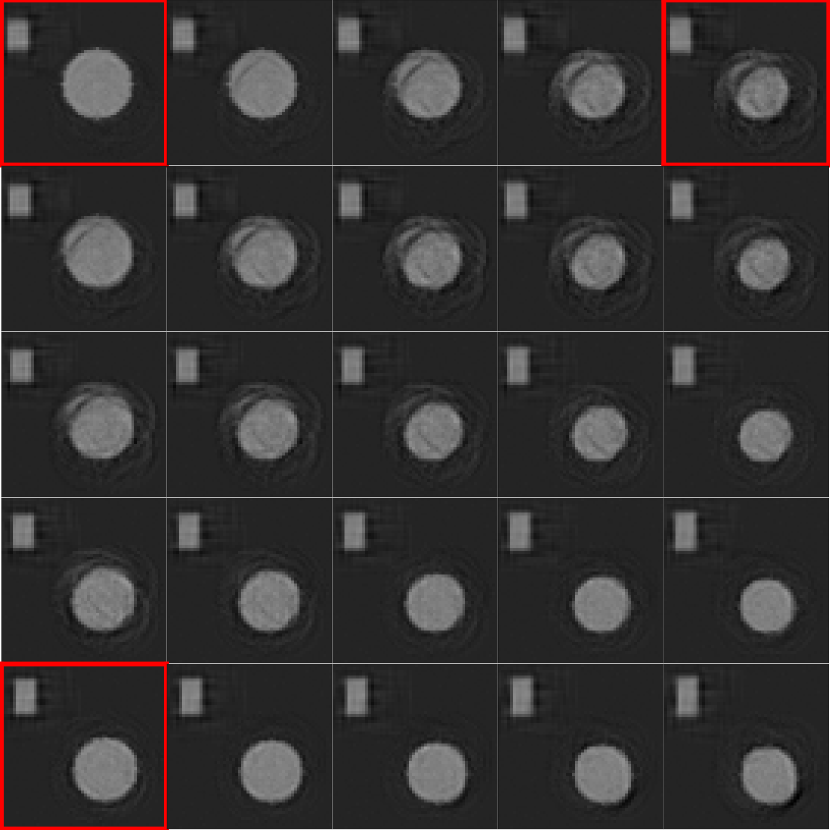
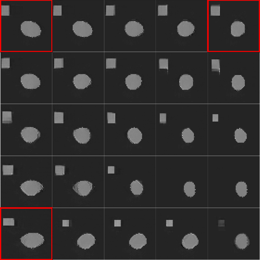
We consider interpolating between points in the latent space, testing property B1. We hope to see smooth transitions between interpolated images, and that generated images are similar to those seen in training. We take three images from the test data, $x_{1},x_{2}$ and $x_{3}$, find $z_{1},z_{2}$ and $z_{3}$, their encodings in the latent space, using (9) and then plot interpolations $G(z_{1}+\alpha_{1}(z_{2}-z_{1})+\alpha_{2}(z_{3}-z_{1}))$ for $\alpha_{1},\alpha_{2}\in[0,1]$. Figure 6 shows one example for each model and dataset for $\alpha_{1},\alpha_{2}=\{0,0.25,0.5,0.75,1\}$. In the AE and VAE, you see transitions that are smooth but blurry. The GAN images appear sharper but some outputs are not similar to training data examples, for example, in Figure 6(f) there are a set of images that contain no rectangle. These images could be evidence of a discriminator failure: the discriminator has not yet learnt that these images are not similar to the training set.

(a) MNIST - AE

(b) MNIST - VAE

(c) MNIST - GAN

(d) Shapes - AE

(e) Shapes - VAE

(f) Shapes - GAN

Figure 6: Interpolation ability of an AE, VAE and GAN. The highlighted top left, bottom left and top right latent space values were chosen close to the test dataset and the other images are computed via linear combinations in the latent space.

4.3.6 Discussion

As expected, none of the three generator models, AE, VAE and GAN, fulfil Property A and B fully. For A, the GAN does poorly in the reconstruction results of Figures 2 and 2. The lack of encoder makes this more challenging. There is evidence of mode collapse, where parts of the training data are not well reconstructed and discriminator failure, where the images produced are not realistic, see Figures 2 and 6. The VAE does consistently better, demonstrated by the lower EMD between generated and test data in Figure 3. The lack of prior on the AE, and thus a known area of the latent space to sample from, is a problem. Figure 5 demonstrates that sampling from the wrong area of the latent space gives poor results.

Pulling apart the cause of a failure to recover an image is difficult. It could be that the image is not in the range of the generator, a failure of Property A, or that the image is in the range of the generator but the image cannot be recovered using descent methods, a failure of Property B. For property B1, the mathematical properties of continuity or differentiability of a network, depend on the architecture. The interpolations in Figure 6 show some evidence of large jumps between images in the GAN cases, but in general the interpolations are reasonable. For both the GAN and the VAE, in Figure 4, the encodings of the test images in the latent space seem to match the prior, Property B2.

5 Numerical Results for Inverse Problems

In this section, we apply AE, VAE and GAN models, evaluated in the previous Section, on three inverse problems. Firstly tomography, the X-ray transform [17] with a parallel beam geometry. Secondly, deconvolution with a $5\times 5$ Gaussian kernel. Lastly, compressed sensing where $y=Ax$ is an under-determined linear system where $A$ is an $\mathbb{R}^{m\times n}$ Gaussian random matrix, $x\in\mathbb{R}^{n}$ is a vectorised image and $n\gg m$, see for example [24]. In each case zero-mean Gaussian noise with standard deviation $\sigma$ is added to the data. The forward operators were implemented using the operator discretisation library (ODL) [2] in Python, accessing scikit–learn [67] for the tomography back-end.

We consider variational regularisation methods in the form of (2) and (7) with $L_{y}(Ax)=\|Ax-y\|_{2}^{2}$. To match the literature themes, we compare three different methods: hard, $F(u)=\iota_{\{0\}}(u)$ and $R_{\mathcal{Z}}(z)=\|z\|_{2}^{2}$; relaxed, $F(u)=\|u\|_{2}^{2}$ and $R_{\mathcal{Z}}(z)=\mu\|z\|_{2}^{2}$; and sparse, $F(u)=\|u\|_{1}$ and $R_{\mathcal{Z}}(z)=\mu\|z\|_{2}^{2}$, where $\mu$ is an additional regularisation parameter. We compare with regularisers independent of the generator: Tikhonov regularisation, $R_{G}(x)=\|x\|_{2}^{2}$, for the convolution and tomography examples and TV regularisation [72], for the compressed sensing example.

The optimisation algorithms are given in the appendix. Hard and Tikhonov are optimised using gradient descent with backtracking line search, Algorithm 1. TV regularisation is implemented using the Primal-Dual Hybrid Gradient method [18]. For relaxed, alternating gradient descent with backtracking is used, see Algorithm 2. Finally, for sparse, the 1-norm is not smooth, and so Proximal Alternating Linearised Minimisation (PALM) [12] with backtracking, Algorithm 3, is used to optimise the equivalent formulation $\min_{u\in\mathcal{X},z\in\mathcal{Z}}\|A(G(z)+u)-y\|_{2}^{2}+\lambda\left(\|u\|_{1}+\mu\|z\|_{2}^{2}\right)$. In all cases, initial values are chosen from a standard normal distribution.

5.1 Deconvolution

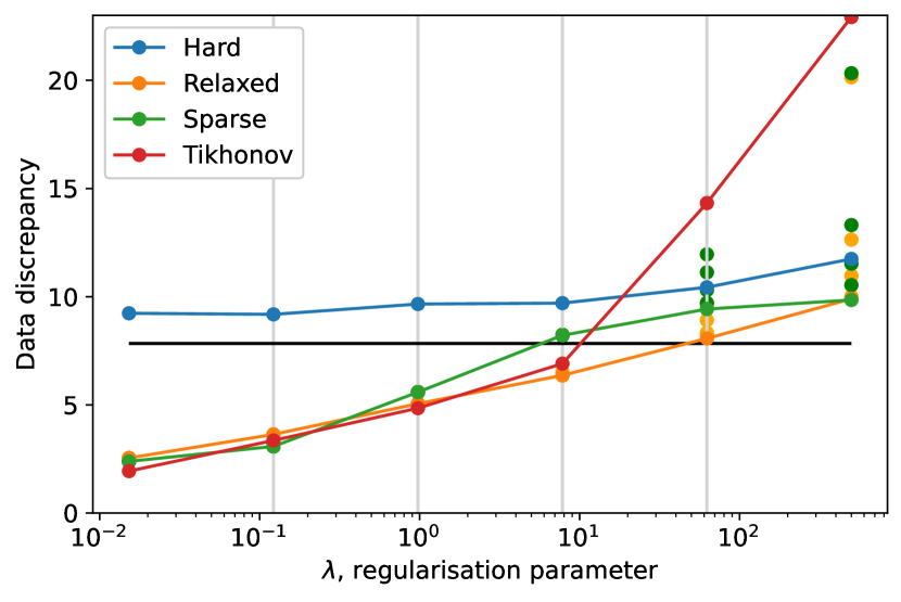
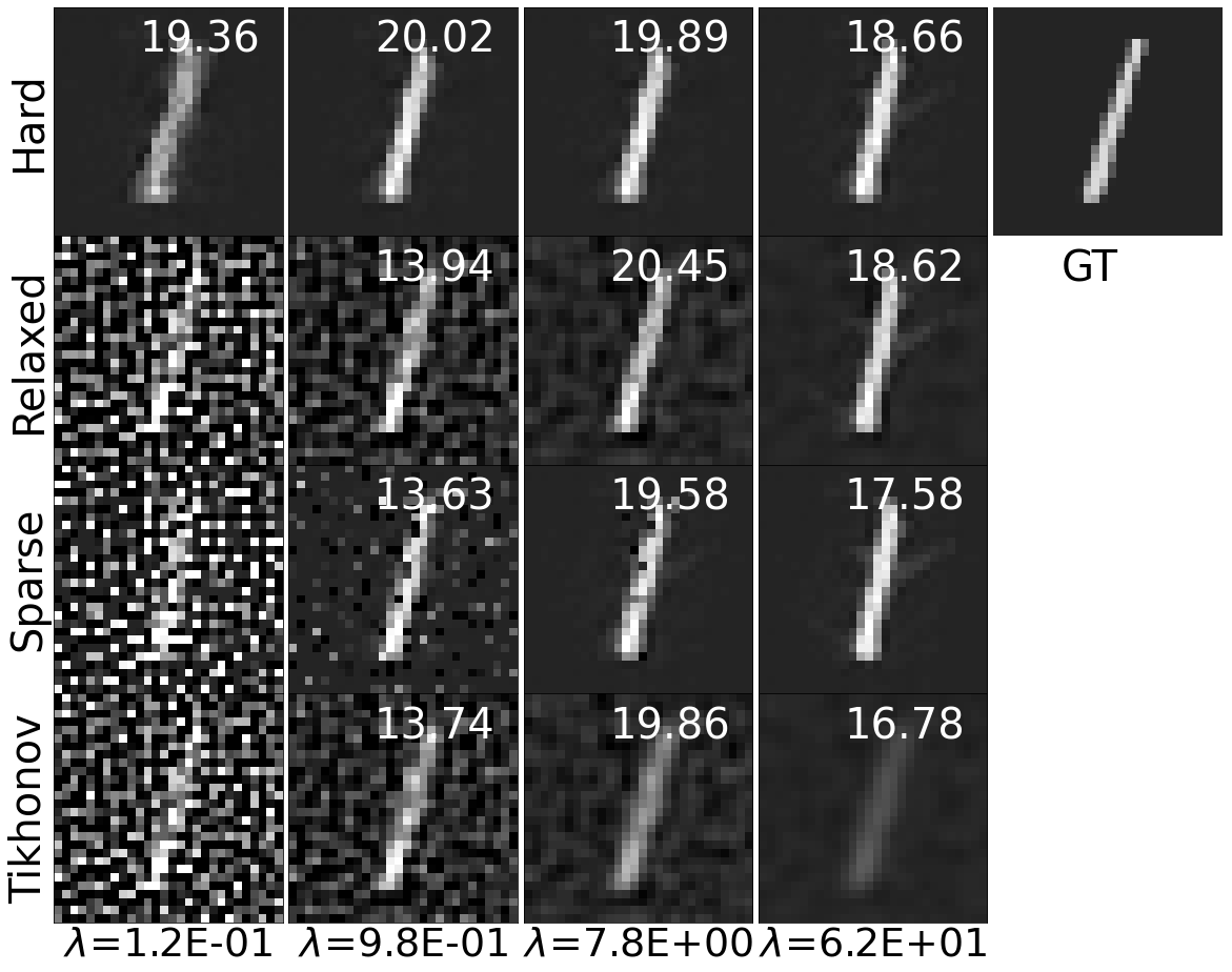
Figure 7 shows solutions to the deconvolution inverse problem with added Gaussian noise (standard deviation $\sigma=0.1$) on the MNIST dataset. We test the relaxed, hard and sparse methods with a GAN against Tikhonov and try a range of regularisation parameters. Each reconstruction used the same realisation of noise affecting the data. Hard gives good PSNR results despite not reaching the Morozov discrepancy value, the expected value of the L2 norm of the added Gaussian noise [79]. For the hard constraints reconstructions are restricted to the range of the generator and we do not expect the data discrepancy to go to zero as $\lambda$ decreases. In the relaxed and sparse constrained reconstructions, for smaller values of $\lambda$ the solutions tend towards a least squares solution which fits the noise and is affected by the ill-posedness of the inverse problem. The additional variation in the choice of $\mu$, as shown by the additional coloured dots, has little effect for smaller values of $\lambda$.

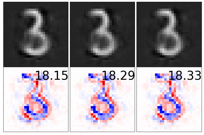
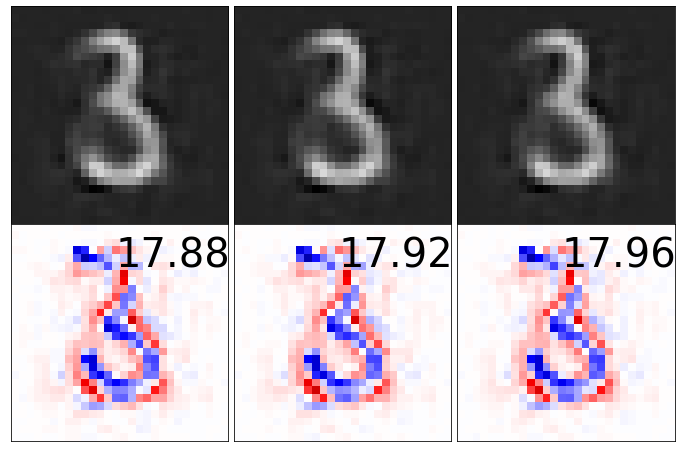
Figure 8 again shows a deconvolution problem with added Gaussian noise (standard deviation $\sigma=0.1$) on the MNIST dataset. We choose the hard reconstruction for the three different generator models and show three random initialisations in $\mathcal{Z}$. Regularisation parameters were chosen to maximise PSNR. The best results are given by the AE and the VAE. The GAN has failed to find a good value in the latent space to reconstruct the number three. The choice of initial value of $z$ significantly affects the outcome of the reconstruction in the GAN case.

Figure 7: Solution of the deconvolution problem on MNIST with an eight-dimensional GAN. The plot shows the L2 reconstruction loss against regularisation parameter choice $\lambda$ in comparison with the Morozov discrepancy value in black. Differing choices for $\mu$ are plotted as additional markers. The image plots correspond to the parameter values shown by the grey lines and include the PSNR values.

(a) GT

(b) AE

(c) VAE

(d) GAN

Figure 8: Comparisons between the three generators, with eight-dimensional latent space, for the deconvolution problem. Reconstructions use the hard method. The plot shows 3 different initialisations for each generator. The ground truth (GT) is given on the left, the top line shows the reconstruction and the bottom line the residuals with the PSNR values.

5.2 Compressed sensing

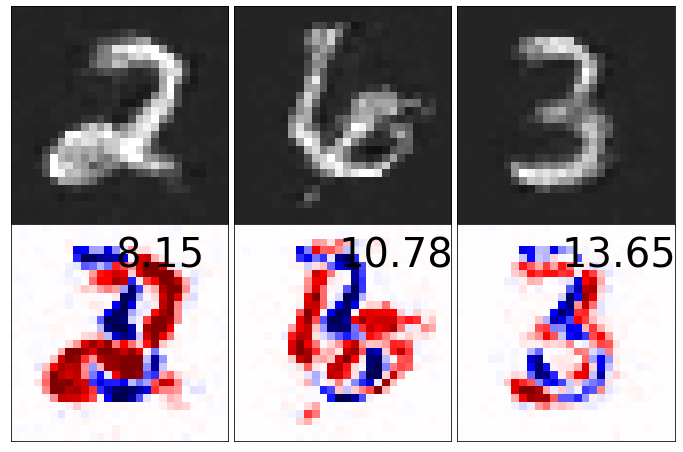
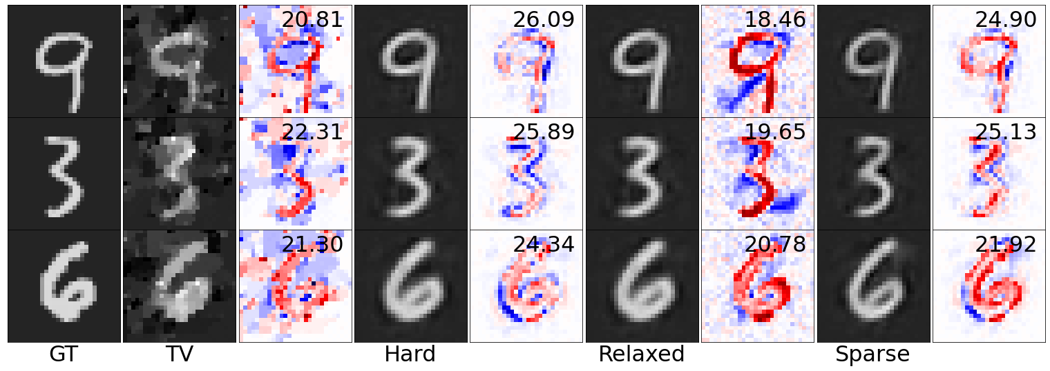
Consider the compressed sensing inverse problem ($m=150$ measurements) with added Gaussian noise (standard deviation $\sigma=0.05$) on MNIST images. We choose regularisation parameters that optimise PSNR over 20 test images. Figure 9 includes a table with the PSNR results on an additional 100 test images. Due to the cartoon like nature of the MNIST digits, TV regularisation is particularly suitable, however VAE and AE hard and VAE relaxed are competitive with TV. For more context, example plots for the the VAE and TV reconstructions are given in Figure 9.

To give an indication of computational cost, Tikhonov reconstruction on the compressed sensing inverse problem on the MNIST dataset took on average 32 iterations of backtracking until the relative difference between iterates was less than $10^{-8}$. In comparison, the hard and relaxed took on average 54 and 325 backtracking steps, respectively, without random restarts. The algorithms took up to 1 second for Tikhonov, 5 seconds for hard and 10 seconds for relaxed.

	Generative Model
Method	AE	VAE	GAN	None
Relaxed	19.31 $\pm$ 2.26	20.07 $\pm$ 1.66	17.12 $\pm$ 1.67
Sparse	19.52 $\pm$ 2.72	21.08 $\pm$ 3.16	17.06 $\pm$ 2.5
Hard	21.84 $\pm$ 4.09	22.33 $\pm$ 4.17	16.93 $\pm$ 2.57
TV				21.54 $\pm$ 1.32

Figure 9: Results compare the three different regularisers and three different methods against the unlearned TV reconstruction on the compressed sensing inverse problem. The table shows the mean and standard deviations of PSNR values of 100 reconstructions. The plots show three example solutions, comparing the VAE reconstructions to TV reconstruction. The left column shows the ground truth, even columns the reconstructed images and odd columns the residuals with the PSNR values.

5.3 Tomography

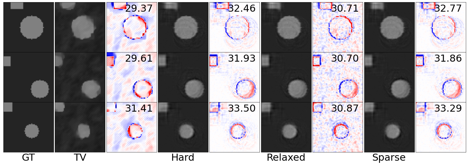
Taking the tomography inverse problem with added Gaussian noise (standard deviation $\sigma=0.1$), Figure 10 includes a table which gives the average and standard deviation for the PSNR of 100 reconstructed Shapes images. The regularisation parameters were set to maximise the PSNR over a separate dataset of 20 test images. The GAN has a particularly poor performance but the AE and VAE results are all competitive with TV. Example reconstructions for the AE methods and TV reconstruction are given in Figure 10. The generative regulariser gives a clear rectangle and circle while the TV reconstruction gives shapes with unclear outlines and blob like artefacts. In terms of computational cost, Tikhonov took on average 157 iterations of backtracking until the relative difference between iterates was less than $10^{-8}$. In comparison, the hard and relaxed took on average 37 and 255 iterations, respectively, without random restarts. The algorithms took up to 40 seconds for Tikhonov, up to 12 seconds for hard and up to 60 seconds for relaxed.

	Generative Model
Method	AE	VAE	GAN	None
Telaxed	30.70 $\pm$ 1.59	28.79 $\pm$ 0.71	24.20 $\pm$ 0.49
Sparse	33.12 $\pm$ 0.80	33.09 $\pm$ 0.89	22.72 $\pm$ 1.80
Hard	33.17 $\pm$ 0.80	32.92 $\pm$ 0.95	22.92 $\pm$ 2.10
TV				$29.94\pm 0.75$

Figure 10: Results compare the three different regularisers and three different methods against the unlearned TV reconstruction on the tomography inverse problem. The table shows the mean and standard deviations of PSNR values of 100 reconstructions. The plots show five example reconstructions, comparing the AE reconstructions to TV reconstruction. The left column shows the ground truth, even columns the reconstructions and odd columns the residuals with the PSNR values.

5.4 Out-of-Distribution Testing

Figure 11: Tomography inverse problem on random images from the shapes+ dataset. It compares the use of sparse method, where sparsity is measured in the TV-norm, with a standard TV reconstruction. The generator is a 10 dimensional VAE trained on Shapes images. In the final column the part of the reconstruction lying in the range of the generator is coloured red and the sparse addition yellow.

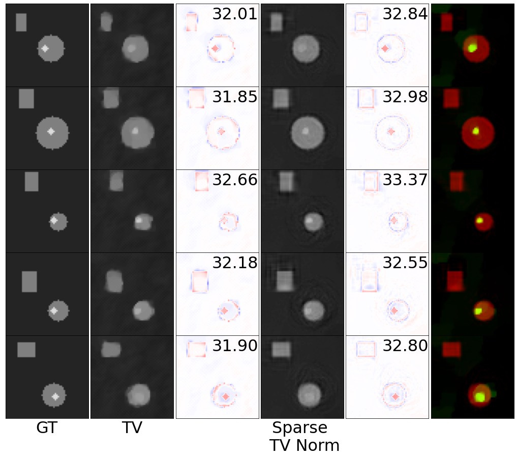
We augment the Shapes dataset, creating a shapes+ dataset, with the addition of a bright spot randomly located in the circle. We then take the Tomography inverse problem on the shapes+ dataset with added Gaussian noise (standard deviation $\sigma=0.05$). For a generative regulariser we use sparse, with $F(x)=\|\nabla x\|_{1}$, the TV norm. Crucially, the VAE generator used was trained only on the standard Shapes dataset, without bright spots. We compare with standard TV reconstruction. The regularisation parameters were chosen to maximise the PSNR on 20 ground truth and reconstructed images. The mean PSNR over 100 test images for the sparse case is 32.83 with standard deviation 0.65 and for the TV reconstruction is 32.01 with standard deviation 0.67. Figure 11 show five reconstructions. The sparse deviations allow reconstruction of the bright spot demonstrating that generative regularisers can also be effective on images close to, but not in, the training distribution.

5.5 FastMRI Dataset

We also train a VAE to produce knee FastMRI images. The VAE architecture is based on Narnhofer et al. The FastMRI knee dataset contains data 796 fully sampled knee MRI magnitude images [50, 87], without fat suppression. We extract 3,872 training and 800 test ground truth images from the dataset, selecting images from near the centre of the knee, resize the images to $128\times 128$ pixels and rescale to the pixel range $[0,1]$. The FastMRI VAE models took approximately 12 hours to train on the same system as above.

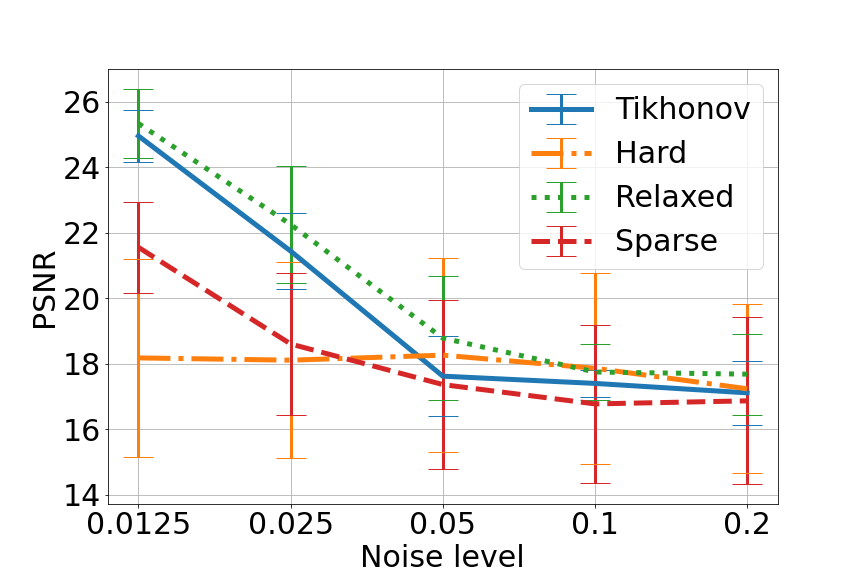
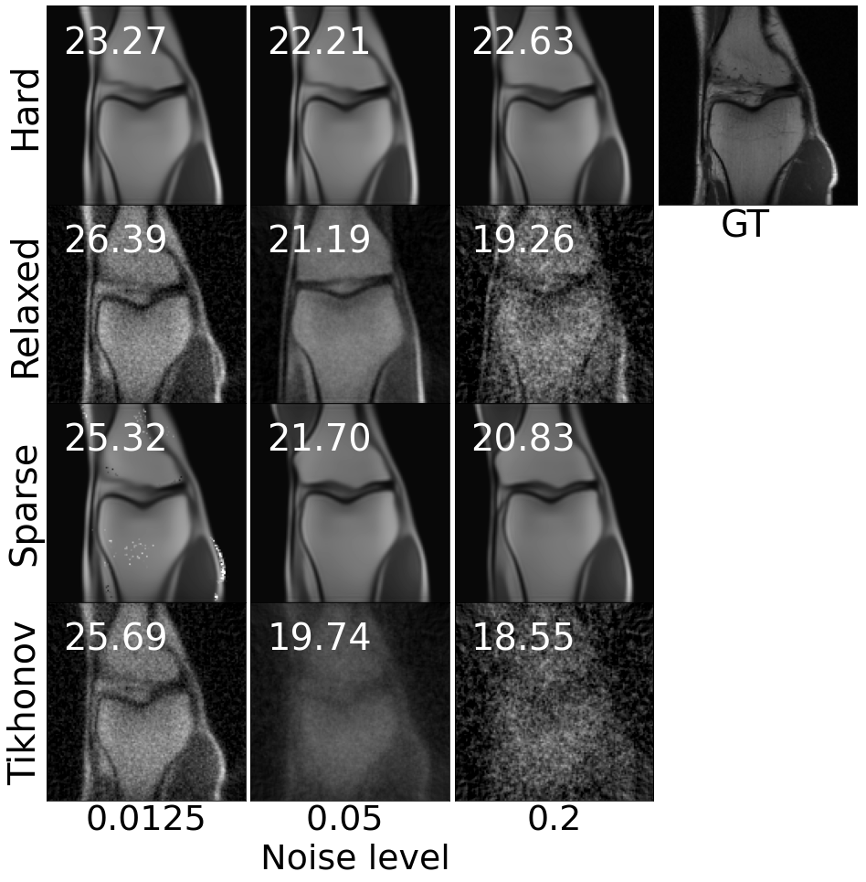
Results for the tomography inverse problem with added Gaussian noise of varying standard deviation are given in Figure 12. For each image and noise level, the same noise instance is used for each reconstruction method, and additionally, for each method, a range of regularisation parameters are tested, and the reconstruction with the best PSNR value chosen. The plot shows how the PSNR values, averaged over 50 test images, vary with noise level. The relaxed method gives the best PSNR values, outperforming Tikhonov although with larger variance. The sparse method curve has a similar shape to Tikhonov, but performs consistently worse suggesting that this choice of deviations from the generator is not suited to this dataset, generator or inverse problem. We see that for the hard method the results are consistent across the range of noise levels, not improving with reduced noise. The example images reflect the data with the hard reconstruction doing comparatively better with larger noise levels, but the relaxed method capturing more of the fine details at the lower noise level.

Figure 12: Reconstructions of the tomography inverse problem with additive Gaussian noise of varying standard deviations. Regularisation parameters are chosen to maximise PSNR value for each image. The left shows the average PSNR values, taken over 50 test images, with the standard deviation in the error bars and the right shows one particular example reconstruction with PSNR values.

6 Summary, Conclusions and Future Work

This paper looked at the use of a generator, from a generative machine learning model, as part of the regulariser of an inverse problem. We named these generative regularisers. Generative regularisers link the theoretically well-understood methods of variational regularisation with state-of-the-art machine learning models. The trained generator outputs data similar to training data and the regulariser restricts solutions (close) to the range of the generator. The cost of these generative regularisers is in the need for generative model training, the requirement for a large amount of training data and the difficulty of the resulting non-convex optimisation scheme. Weighing up the costs and benefits will depend on the inverse problem and the availability of data.

We compared three different types of generative regularisers which either restrict solutions to exactly the range of the generator or allow small or sparse deviations. We found that in simpler datasets the restriction to the range of the generator was successful. Where the ground truth was more complex then allowing small deviations produced the best results. A key benefit of generative regularisers over other deep learning approaches is that paired training data is not required, making the method flexible to changes in the forward problem. We demonstrated the use of generative regularisers on deconvolution and fully sampled tomography problems, both with gradually decaying singular values of the forward operator; and compressed sensing, with a large kernel and non-unique solutions.

The training of the generator is crucial to the success of generative regularisers, and a key contribution of this report is a set of desirable properties for a generator. Numerical tests linked to these properties were discussed and applied to three generative models: AEs, VAEs and GANs. None of these models fulfil the criteria completely. We observed known issues such as mode collapse and discriminator failure in the GAN, blurry images in the VAE and the lack of a prior in the AE. In the inverse problem experiments in this paper the AE and the VAE yielded the most consistent results. The success of the AE, despite the lack of prior on the latent space, surprised us. We suspect the implicit regularisation on the model from the architecture and initialisations helped making the AE a usable generator. The GAN models did worst in the inverse problem examples: they generally seemed more sensitive to initialisation of the non convex optimisation, making the optimal point in the latent space difficult to recover.

This paper focused on training the generative model first and then subsequently using the generative regularisation to solve inverse problems. The benefit of this split approach is that the model does not need retraining if there are changes in the forward problem. A further advantage is that the field of generative modelling is growing quickly and any improvements to generators can be directly plugged into these methods. An interesting direction for future work would be to consider training (or refining) generative models with a particular inverse problem in mind.

Appendix A Optimisation Algorithms

Algorithm 1 Gradient Descent with Backtracking to solve $\min_{z}f(z)$.

1:Initialise $z_{0}$, $L>0$, $0<\eta_{0}<1$, $\eta_{1}>1$.

2:for $i=1,...,K$ do

3:     Let $\tilde{z}(L):=z_{i-1}-\frac{1}{L}\nabla f(z_{i-1})$

4:     while $f(\tilde{z}(L))\geq f(z_{i-1})-\frac{1}{2L}\|\nabla f(z_{i-1})\|_{2}^{2}$ do

5:         $L=L\eta_{1}$      

6:     $z_{i}=\tilde{z}$ and $L=L\eta_{0}$.

Algorithm 2 Alternating gradient descent with backtracking to solve $\min_{z,x}f(z,x)$.

1:Initialise $z_{0}$ and $x_{0}$, $L_{z}>0$,$L_{x}>0$, $0<\eta_{0}<1$ and $\eta_{1}>1$

2:for $i=1,....,K$ do

3:     Let $\tilde{z}(L_{z}):=z_{i}-\frac{1}{L_{z}}\nabla f(z_{i},x_{i})$

4:     while $f(\tilde{z}(L_{z}),x_{i})\geq f(z_{i},x_{i})-\frac{1}{2L_{z}}\|\nabla f(z_{i},x_{i})\|_{2}^{2}$ do

5:         $L_{z}=L_{z}\eta_{1}$      

6:     Let $z_{i+1}=\tilde{z}(L_{z})$ and then $L_{z}=L_{z}\eta_{0}$

7:     Let $\tilde{x}(L_{x}):=x_{i}-\frac{1}{L_{x}}\nabla f(z_{i+1},x_{i})$

8:     while $f(z_{i+1},\tilde{x}(L_{x}))\geq f(z_{i+1},x_{i})-\frac{1}{2L_{x}}\|\nabla f(z_{i+1},x_{i})\|_{2}^{2}$ do

9:         $L_{x}=L_{x}\eta_{1}$      

10:     Let $x_{i+1}=\tilde{x}(x_{L})$ and $L_{x}=L_{x}\eta_{0}$

Algorithm 3 PALM with backtracking to solve $\min_{z,u}f(z,u)+g_{1}(z)+g_{2}(u)$. Define $\mathrm{prox}_{h}(z)=\arg\min_{x}\{h(x)+\frac{1}{2}\|x-z\|_{2}^{2}\}$.

1:Initialise $z_{0}$, $u_{0}$, $L_{z}>0$, $L_{x}>0$, $0<\eta_{0}<1$ and $\eta_{1}>1$.

2:for $i=1,...K$ do

3:     Let $\tilde{z}(L_{z}):=\mathrm{prox}_{\frac{1}{L_{z}}g_{1}}(z_{i}-\frac{1}{L_{z}}\nabla_{z}f(z_{i},u_{i}))$

4:     while $f(\tilde{z}(L_{z}),u_{i})>f(z_{i},u_{i})+\nabla_{z}f(z_{i},u_{i})^{T}(\tilde{z}(L_{z})-u_{i})+\frac{L_{z}}{2}\|\tilde{z}(L_{z})-z_{i}\|_{2}^{2}$ do

5:         $L_{z}=L_{z}\eta_{1}$      

6:     Let $z_{i+1}=\tilde{z}(L_{z})$ and then $L_{z}=L_{z}\eta_{0}$

7:     Let $\tilde{u}(L_{u}):=\mathrm{prox}_{\frac{1}{L_{u}}g_{2}}(u_{i}-\frac{1}{L_{u}}\nabla_{u}f(z_{i+1},u_{i}))$

8:     while $f(z_{i+1},\tilde{u}(L_{u}))>f(z_{i+1},u_{i})+\nabla_{u}f(z_{i+1},u_{i})^{T}(\tilde{u}(L_{u})-u_{i})+\frac{L_{u}}{2}\|\tilde{u}(L_{u})-u_{i}\|_{2}^{2}$ do      

9:     Let $u_{i+1}=\tilde{u}(L_{u})$ and then set $L_{u}=L_{u}\eta_{0}$

Appendix B Generative Model Architectures

The architectures for the three different generative models, for the different datasets are given in this Appendix.

Figure 13: Definitions used in Figure 14, 15 and 16.

Figure 14: The architectures for the 3 generative models, AE, VAE and GAN, for the MNIST dataset. The convolution block definitions are given in Figure 13.

Figure 15: The architectures for the 3 generative models, AE, VAE and GAN, for the Shapes dataset. The convolution block definitions are given in Figure 13.

Figure 16: The architectures for the knee dataset VAE. The convolution block definitions are given in Figure 13.

References

- [1] Jonas Adler and Ozan Öktem “Deep Bayesian Inversion” In ArXiv Preprint, 2018 arXiv: http://arxiv.org/abs/1811.05910
- [2] Jonas Adler, Holger Kohr and Ozan Öktem “Operator Discretization Library (ODL)”, 2017 URL: https://doi.org/10.5281/zenodo.249479
- [3] Michal Aharon, Michael Elad and Alfred Bruckstein “K-SVD: An algorithm for designing overcomplete dictionaries for sparse representation” In IEEE Transactions on Signal Processing 54.11, 2006, pp. 4311–4322 DOI: 10.1109/TSP.2006.881199
- [4] Rushil Anirudh, Jayaraman J. Thiagarajan, Bhavya Kailkhura and Timo Bremer “An Unsupervised Approach to Solving Inverse Problems using Generative Adversarial Networks” In ArXiv Preprint, 2018 arXiv: http://arxiv.org/abs/1805.07281
- [5] Martin Arjovsky, Soumith Chintala and Léon Bottou “Wasserstein generative adversarial networks” In ICML, 2017, pp. 298–321
- [6] Sanjeev Arora, Andrej Risteski and Yi Zhang “Do GANs Learn the Distribution? Some Theory and Empirics” In ICLR, 2018, pp. 1–16
- [7] Simon Arridge, Peter Maass, Ozan Öktem and Carola Bibiane Schönlieb “Solving inverse problems using data-driven models” In Acta Numerica 28, 2019, pp. 1–174
- [8] Muhammad Asim, Fahad Shamshad and Ali Ahmed “Blind image deconvolution using pretrained generative priors” In BMVC, 2020 URL: http://arxiv.org/abs/1908.07404
- [9] Matthias Bauer and Andriy Mnih “Resampled priors for variational autoencoders” In AISTATS 2019 - 22nd International Conference on Artificial Intelligence and Statistics PMLR, 2020, pp. 66–75
- [10] Martin Benning and Martin Burger “Modern regularization methods for inverse problems” In Acta Numerica 27.27, 2018, pp. 1–111 DOI: 10.1017/S0962492918000016
- [11] Yoeri E. Boink and Christoph Brune “Learned SVD: solving inverse problems via hybrid autoencoding” In ArXiv Preprint, 2019 arXiv: http://arxiv.org/abs/1912.10840
- [12] Jérôme Bolte, Shoham Sabach and Marc Teboulle “Proximal alternating linearized minimization for nonconvex and nonsmooth problems” In Mathematical Programming 146.1-2, 2014, pp. 459–494 DOI: 10.1007/s10107-013-0701-9
- [13] Ashish Bora, Ajil Jalal, Eric Price and Alexandros G. Dimakis “Compressed sensing using generative models” In ICML, 2017, pp. 822–841
- [14] Ali Borji “Pros and cons of GAN evaluation measures” In Computer Vision and Image Understanding 179, 2019, pp. 41–65 DOI: 10.1016/j.cviu.2018.10.009
- [15] Kristian Bredies and Dirk Lorenz “Mathematical image processing” In Applied and Numerical Harmonic Analysis Springer International Publishing, 2018, pp. 1–469
- [16] Emmanuel J. Candes and Terence Tao “Decoding by linear programming” In IEEE Transactions on Information Theory 51.12, 2005, pp. 4203–4215
- [17] Yair Censor “The mathematics of computerized tomography” In Inverse Problems 18.1 SIAM, 2002, pp. 283 DOI: 10.1088/0266-5611/18/1/601
- [18] Antonin Chambolle and Thomas Pock “A first-order primal-dual algorithm for convex problems with applications to imaging” In Journal of Mathematical Imaging and Vision 40.1 Springer, 2011, pp. 120–145 DOI: 10.1007/s10851-010-0251-1
- [19] Paramanand Chandramouli et al. “Generative Models for Generic Light Field Reconstruction” In TPAMI, 2020 URL: http://arxiv.org/abs/2005.06508
- [20] Bin Dai and David Wipf “Diagnosing and enhancing VAE models” In 7th International Conference on Learning Representations, ICLR 2019, 2019 URL: https://github.com/daib13/TwoStageVAE.
- [21] Giannis Daras, Joseph Dean, Ajil Jalal and Alexandros G. Dimakis “Intermediate Layer Optimization for Inverse Problems using Deep Generative Models” In International Conference on Machine Learning (ICML), 2021
- [22] Constantinos Daskalakis, Dhruv Rohatgi and Manolis Zampetakis “Constant-expansion suffices for compressed sensing with generative priors” In Advances in Neural Information Processing Systems 2020-Decem, 2020 URL: https://arxiv.org/abs/2006.04237
- [23] Akshat Dave et al. “Solving Inverse Computational Imaging Problems Using Deep Pixel-Level Prior” In IEEE Transactions on Computational Imaging 5.1, 2018, pp. 37–51 DOI: 10.1109/tci.2018.2882698
- [24] Mark A. Davenport, Marco F. Duarte, Yonina C. Eldar and Gitta Kutyniok “Introduction to compressed sensing” In Compressed Sensing: Theory and Applications Citeseer, 2009, pp. 1–64 DOI: 10.1017/CBO9780511794308.002
- [25] Manik Dhar, Aditya Grover and Stefano Ermon “Modeling Sparse Deviations for Compressed Sensing using Generative Models” In ICML 3, 2018, pp. 1990–2005
- [26] Sören Dittmer, Tobias Kluth, Peter Maass and Daniel Otero Baguer “Regularization by Architecture: A Deep Prior Approach for Inverse Problems” In Journal of Mathematical Imaging and Vision 62.3 JMIV, 2020, pp. 456–470 DOI: 10.1007/s10851-019-00923-x
- [27] Rémi Flamary and Nicolas Courty “POT python optimal transport library” In GitHub: https://github. com/rflamary/POT 22, 2017, pp. 1–8 URL: https://pythonot.github.io/
- [28] Mario González et al. “Solving Inverse Problems by Joint Posterior Maximization with a VAE Prior” In ArXiv Preprint, 2019 arXiv: http://arxiv.org/abs/1911.06379
- [29] Ian J. Goodfellow et al. “Generative adversarial nets” In NeurIPS, 2014, pp. 2672–2680
- [30] GoogleResearch “TensorFlow: Large-scale machine learning on heterogeneous systems”, 2015 arXiv: http://download.tensorflow.org/paper/whitepaper2015.pdf
- [31] Arthur Gretton et al. “A Kernel Two-Sample Test” In JMLR 13, 2012, pp. 723–773 URL: www.gatsby.ucl.ac.uk/
- [32] Jinjin Gu, Yujun Shen and Bolei Zhou “Image processing using multi-code GaN prior” In CVPR, 2020, pp. 3009–3018
- [33] Ishaan Gulrajani et al. “Improved training of wasserstein GANs” In NeurIPS, 2017, pp. 5768–5778
- [34] Sean Gunn, Jorio Cocola and Paul Hand “Regularized Training of Intermediate Layers for Generative Models for Inverse Problems”, 2022 DOI: 10.48550/arxiv.2203.04382
- [35] Harshit Gupta, Michael T. McCann, Laurene Donati and Michael Unser “CryoGAN: A New Reconstruction Paradigm for Single-Particle Cryo-EM Via Deep Adversarial Learning” In IEEE Transactions on Computational Imaging, 2021 DOI: 10.1109/TCI.2021.3096491
- [36] Andreas Habring and Martin Holler “A Generative Variational Model for Inverse Problems in Imaging” In SIAM Journal on Mathematics of Data Science 4.1, 2022, pp. 306–335
- [37] Paul Hand and Vladislav Voroninski “Global Guarantees for Enforcing Deep Generative Priors by Empirical Risk” In IEEE Transactions on Information Theory 66.1, 2020, pp. 401–418 DOI: 10.1109/TIT.2019.2935447
- [38] Paul Hand, Oscar Leong and Vladislav Voroninski “Phase retrieval under a generative prior” In NeurIPS, 2018, pp. 9136–9146
- [39] Chinmay Hegde “Algorithmic Aspects of Inverse Problems Using Generative Models” In 56th Annual Allerton Conference on Communication, Control, and Computing, 2019, pp. 166–172 DOI: 10.1109/ALLERTON.2018.8636031
- [40] Martin Heusel et al. “GANs trained by a two time-scale update rule converge to a local Nash equilibrium” In NeurIPS, 2017, pp. 6627–6638 URL: https://arxiv.org/abs/1706.08500
- [41] Shady Abu Hussein, Tom Tirer and Raja Giryes “Image-Adaptive GAN based Reconstruction” In AAAI 2020 - 34th AAAI Conference on Artificial Intelligence, 2019, pp. 3121–3129
- [42] Kazufumi Ito and Bangti Jin “Inverse Problems: Tikhonov Theory And Algorithms (Applied Mathematics)” In Series on Applied Mathematics, 2014
- [43] Jörn Henrik Jacobsen, Arnold Smeulders and Edouard Oyallon “I-RevNet: Deep invertible networks” In ICLR, 2018
- [44] Gauri Jagatap and Chinmay Hegde “Algorithmic guarantees for inverse imaging with untrained network priors” In NeurIPS 32, 2019
- [45] Ajil Jalal et al. “Robust Compressed Sensing MRI with Deep Generative Priors”, 2021 DOI: 10.48550/arxiv.2108.01368
- [46] Maya Kabkab, Pouya Samangouei and Rama Chellappa “Task-aware compressed sensing with generative adversarial networks” In AAAI, 2018, pp. 2297–2304
- [47] Diederik P. Kingma and Prafulla Dhariwal “Glow: Generative flow with invertible 1×1 convolutions” In Advances in Neural Information Processing Systems, 2018, pp. 10215–10224
- [48] Diederik P. Kingma and Max Welling “An introduction to variational autoencoders” In Foundations and Trends in Machine Learning 12.4, 2019, pp. 307–392 DOI: 10.1561/2200000056
- [49] Diederik P. Kingma and Max Welling “Auto-encoding variational bayes” In ICLR, 2014
- [50] Florian Knoll et al. “fastMRI: A Publicly Available Raw k-Space and DICOM Dataset of Knee Images for Accelerated MR Image Reconstruction Using Machine Learning” In Radiology: Artificial Intelligence 2.1, 2020, pp. e190007 DOI: 10.1148/ryai.2020190007
- [51] Avisek Lahiri, Arnav Kumar Jain, Divyasri Nadendla and Prabir Kumar Biswas “Faster Unsupervised Semantic Inpainting: A GAN Based Approach” In ICIP, 2019, pp. 2706–2710 DOI: 10.1109/ICIP.2019.8803356
- [52] Yann LeCun, Léon Bottou, Yoshua Bengio and Patrick Haffner “Gradient-based learning applied to document recognition” In Proceedings of the IEEE 86.11, 1998, pp. 2278–2323 DOI: 10.1109/5.726791
- [53] Qi Lei, Ajil Jalal, Inderjit S. Dhillon and Alexandros G. Dimakis “Inverting deep generative models, one layer at a time” In NeurIPS 32, 2019
- [54] Housen Li, Johannes Schwab, Stephan Antholzer and Markus Haltmeier “NETT: Solving inverse problems with deep neural networks” In Inverse Problems 36.6, 2020 DOI: 10.1088/1361-6420/ab6d57
- [55] David Lopez-Paz and Maxime Oquab “Revisiting classifier two-sample tests” In ICLR, 2017
- [56] Sebastian Lunz, Ozan Öktem and Carola Bibiane Schönlieb “Adversarial regularizers in inverse problems” In NeurIPS, 2018, pp. 8507–8516
- [57] Jun Lv, Jin Zhu and Guang Yang “Which GAN? A comparative study of generative adversarial network-based fast MRI reconstruction” In Philosophical Transactions of the Royal Society A: Mathematical, Physical and Engineering Sciences 379.2200 The Royal Society Publishing, 2021 DOI: 10.1098/rsta.2020.0203
- [58] Tim Meinhardt, Michael Moeller, Caner Hazirbas and Daniel Cremers “Learning Proximal Operators: Using Denoising Networks for Regularizing Inverse Imaging Problems” In ICCV, 2017, pp. 1799–1808
- [59] Sachit Menon et al. “PULSE: Self-Supervised Photo Upsampling via Latent Space Exploration of Generative Models” In CVPR, 2020, pp. 2437–2445 DOI: 10.1109/cvpr42600.2020.00251
- [60] Lukas Mosser, Olivier Dubrule and Martin J. Blunt “Stochastic Seismic Waveform Inversion Using Generative Adversarial Networks as a Geological Prior” In Mathematical Geosciences 52.1, 2020, pp. 53–79 DOI: 10.1007/s11004-019-09832-6
- [61] Dominik Narnhofer, Kerstin Hammernik, Florian Knoll and Thomas Pock “Inverse GANs for accelerated MRI reconstruction” SPIE-Intl Soc Optical Eng, 2019, pp. 45
- [62] Thomas Oberlin and Mathieu Verm “Regularization Via Deep Generative Models: an Analysis Point of View” In ICIP, 2021, pp. 404–408
- [63] Daniel Obmann, Johannes Schwab and Markus Haltmeier “Deep synthesis regularization of inverse problems” In ArXiv Preprint, 2020 arXiv: http://arxiv.org/abs/2002.00155
- [64] Daniel Obmann, Linh Nguyen, Johannes Schwab and Markus Haltmeier “Sparse Anett for Solving Inverse Problems with Deep Learning” In International Symposium on Biomedical Imaging Workshops, Proceedings, 2020 DOI: 10.1109/ISBIWorkshops50223.2020.9153362
- [65] Gyutaek Oh et al. “Unpaired Deep Learning for Accelerated MRI Using Optimal Transport Driven CycleGAN” In IEEE Transactions on Computational Imaging, 2020, pp. 1285–1296
- [66] Hyoung Suk Park et al. “Unpaired image denoising using a generative adversarial network in x-ray CT” In IEEE Access 7, 2019, pp. 110414–110425 DOI: 10.1109/ACCESS.2019.2934178
- [67] Fabian Pedregosa et al. “Scikit-learn: Machine Learning in Python” In JMLR 12, 2011, pp. 2825–2830
- [68] Pei Peng, Shirin Jalali and Xin Yuan “Auto-encoders for compressed sensing” In NeurIPS, 2019
- [69] Zaccharie Ramzi et al. “Denoising Score-Matching for Uncertainty Quantification in Inverse Problems” In NeurIPS, 2020
- [70] Yaniv Romano, Michael Elad and Peyman Milanfar “The little engine that could: Regularization by Denoising (RED)” In SIAM Journal on Imaging Sciences 10.4, 2017, pp. 1804–1844 DOI: 10.1137/16M1102884
- [71] Yossi Rubner, Carlo Tomasi and Leonidas J. Guibas “Metric for distributions with applications to image databases” In ICCV, 1998, pp. 59–66 DOI: 10.1109/iccv.1998.710701
- [72] Leonid I. Rudin, Stanley Osher and Emad Fatemi “Nonlinear total variation based noise removal algorithms” In Physica D: Nonlinear Phenomena 60.1-4, 1992, pp. 259–268
- [73] Tim Salimans et al. “Improved techniques for training GANs” In NeurIPS, 2016, pp. 2234–2242
- [74] Otmar Scherzer et al. “Variational regularization methods for the solution of inverse problems” In Applied Mathematical Sciences (Switzerland) 167 Springer, 2009, pp. 53–113
- [75] Viraj Shah and Chinmay Hegde “Solving Linear Inverse Problems Using Gan Priors: An Algorithm with Provable Guarantees” In ICASSP, 2018, pp. 4609–4613
- [76] Byeongsu Sim, Gyutaek Oh and Jong Chul Ye “Optimal Transport Structure of CycleGAN for Unsupervised Learning for Inverse Problems” In ICASSP, 2020, pp. 8644–8647 DOI: 10.1109/ICASSP40776.2020.9053125
- [77] Yang Song and Stefano Ermon “Improved techniques for training score-based generative models” In NeurIPS, 2020
- [78] Lucas Theis, Aäron Van Den Oord and Matthias Bethge “A note on the evaluation of generative models” In ICLR, 2016 URL: http://arxiv.org/abs/1511.01844https://arxiv.org/abs/1511.01844
- [79] A. N. Tikhonov, A. V. Goncharsky, V. V. Stepanov and A. G. Yagola “Numerical Methods for the Solution of Ill-Posed Problems” In Numerical Methods for the Solution of Ill-Posed Problems, 1995 DOI: 10.1007/978-94-015-8480-7
- [80] Subarna Tripathi, Zachary C. Lipton and Truong Q. Nguyen “Correction by Projection: Denoising Images with Generative Adversarial Networks” In ArXiv Preprint, 2018 arXiv:1803.04477
- [81] Dmitry Ulyanov, Andrea Vedaldi and Victor Lempitsky “Deep Image Prior” In International Journal of Computer Vision, 2020, pp. 1867–1888
- [82] Dave Van Veen et al. “Compressed Sensing with Deep Image Prior and Learned Regularization” In ArXiv Preprint, 2018 arXiv: http://arxiv.org/abs/1806.06438
- [83] Singanallur V. Venkatakrishnan, Charles A. Bouman and Brendt Wohlberg “Plug-and-Play priors for model based reconstruction” In GlobalSIP, 2013, pp. 945–948 DOI: 10.1109/GlobalSIP.2013.6737048
- [84] Tom White “Sampling Generative Networks” In ArXiv Preprint, 2016 arXiv: http://arxiv.org/abs/1609.04468
- [85] Guang Yang et al. “DAGAN: Deep De-Aliasing Generative Adversarial Networks for Fast Compressed Sensing MRI Reconstruction” In IEEE Transactions on Medical Imaging 37.6 Institute of ElectricalElectronics Engineers Inc., 2018, pp. 1310–1321 DOI: 10.1109/TMI.2017.2785879
- [86] Raymond A. Yeh et al. “Semantic image inpainting with deep generative models” In CVPR IEEE, 2017, pp. 6882–6890 DOI: 10.1109/CVPR.2017.728
- [87] Jure Zbontar et al. “fastMRI: An Open Dataset and Benchmarks for Accelerated MRI” In ArXiv Preprint, 2018 arXiv:1811.08839
- [88] Jun Yan Zhu, Taesung Park, Phillip Isola and Alexei A. Efros “Unpaired Image-to-Image Translation Using Cycle-Consistent Adversarial Networks” In ICCV, 2017, pp. 2242–2251