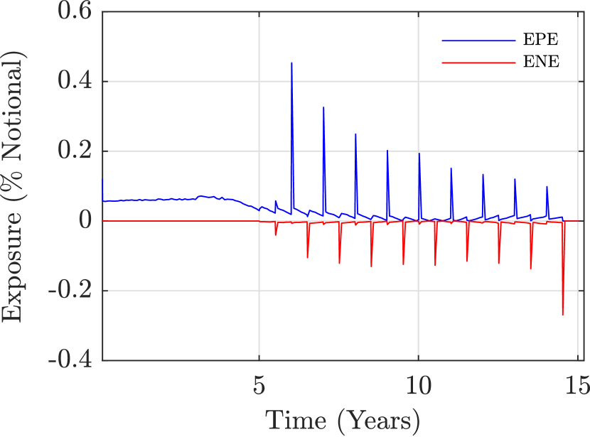
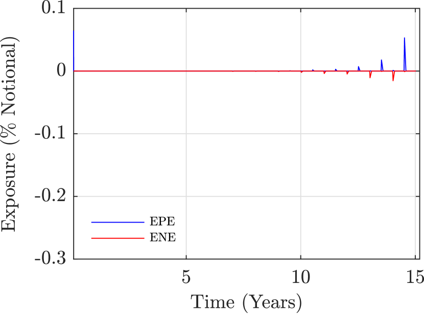
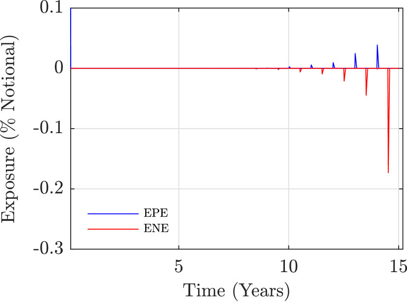
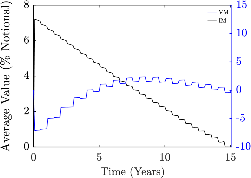
Everything You Always Wanted to Know About XVA Model Risk but Were Afraid to Ask

Lorenzo Silotto111Deloitte Consulting S.r.l., silotto.lorenzo@gmail.com Marco Scaringi222Intesa Sanpaolo, Financial and Market Risk Management, marco.scaringi@intesasanpaolo.com Marco Bianchetti333Intesa Sanpaolo, Financial and Market Risk Management, and University of Bologna, Department of Statistical Sciences “Paolo Fortunati”, marco.bianchetti@unibo.it
(March 8, 2024)
Abstract

Valuation adjustments, collectively named XVA, play an important role in modern derivatives pricing. XVA are an exotic pricing component since they require the forward simulation of multiple risk factors in order to compute the portfolio exposure including collateral, leading to a significant model risk and computational effort, even in case of plain vanilla trades.

This work analyses the most critical model risk factors, meant as those to which XVA are most sensitive, finding an acceptable compromise between accuracy and performance. This task has been conducted in a complete context including a market standard multi-curve G2++ model calibrated on real market data, both Variation Margin and ISDA-SIMM dynamic Initial Margin, different collateralization schemes, and the most common linear and non-linear interest rates derivatives. Moreover, we considered an alternative analytical approach for XVA in case of uncollateralized Swaps.

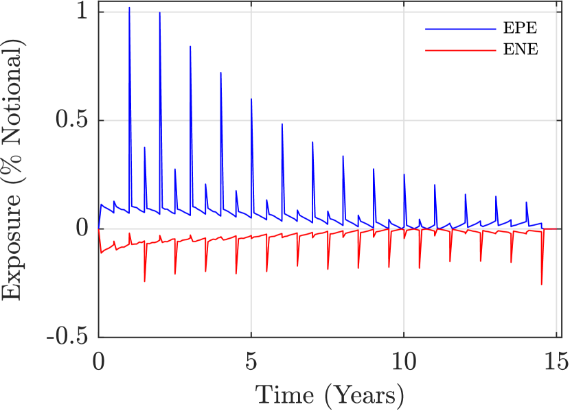
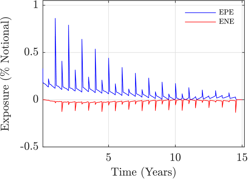
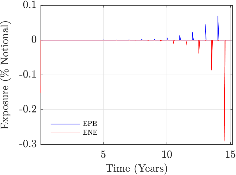
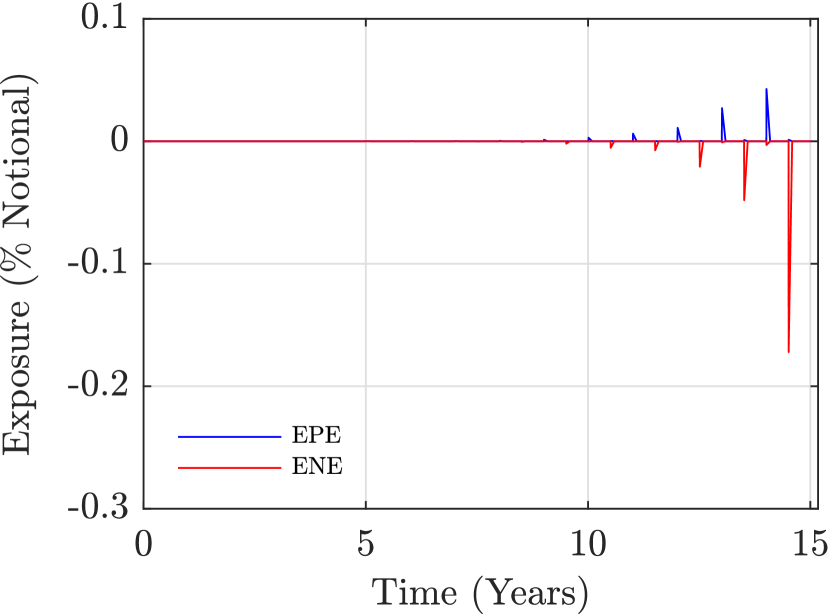
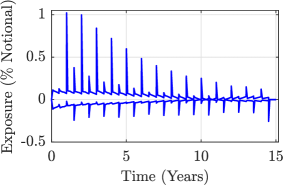
We show that a crucial element is the construction of a parsimonious time grid capable of capturing all periodical spikes arising in collateralized exposure during the Margin Period of Risk. To this end, we propose a workaround to efficiently capture all spikes. Moreover, we show that there exists a parameterization which allows to obtain accurate results in a reasonable time, which is a very important feature for practical applications. In order to address the valuation uncertainty linked to the existence of a range of different parameterizations, we calculate the Model Risk AVA (Additional Valuation Adjustment) for XVA according to the provisions of the EU Prudent Valuation regulation.

Finally, this work can serve as an handbook containing step-by-step instructions for the implementation of a complete, realistic and robust modelling framework of collateralized exposure and XVA.

JEL classifications: G10, G12, G13, G15, G18, G20, G33.

Keywords: Interest Rates, XVA, CVA, DVA, AVA, Prudent Valuation, Model Risk, Market Risk, Counterparty Risk, Model Validation, Credit Exposure, Variation Margin, Initial Margin, ISDA-SIMM, Swaps, Swaptions, Derivatives.

Acknowledgements: the authors acknowledge fruitful discussions with Marcello Terraneo, Andrea Principe, and many other colleagues in Intesa Sanpaolo Risk Management Department.

Disclaimer: the views expressed here are those of the authors and do not represent the opinions of their employers. They are not responsible for any use that may be made of these contents.

1 Introduction

The 2007 credit crunch crisis has made necessary to reconsider the methodologies used until that time to price over-the-counter (OTC) derivatives. For example, during the crisis a change of regime in the interest rate market was observed: basis spreads between interest rate derivatives characterised by different underlying rate tenors (e.g. IBOR 3M444IBOR denotes a generic Interbank Offered Rates., IBOR 6M, etc.) exploded and the spread between Overnight Indexed Swap (OIS) rates and rates of longer tenors widened significantly. This change of regime has lead to an evolution of market practice with the introduction of multiple interest rate yield curves (multi-curve framework) and OIS discounting. Literature is very extensive in this field, a non-exhaustive list of references is [1, 2, 3, 4, 5, 6, 7]. Such framework has been recently questioned by the interest benchmark reform and the progressive replacement of the old IBOR rates with the corresponding risk free rates. Benchmark reform impacts XVA as well, but in this paper it is not considered at all. We refer to [8] for a discussion around the impact of EONIA-€STR discounting switch on XVA.

Moreover, the crisis triggered the incorporation of additional risk factors within the usual risk-neutral valuation through a set of valuation adjustments, collectively named XVA. In particular, the Lehman Brothers bankruptcy triggered a greater awareness amongst market participants on counterparty credit risk, leading to its inclusion in derivatives pricing via Credit Valuation Adjustment (CVA)555Which actually was explored before the crisis, see e.g. [9] and references therein.. Post-crisis also the own risk of default began to be addressed (see e.g. [10, 11]) leading to bilateral CVA models and Debt Valuation Adjustment (DVA). Both CVA and DVA are also envisaged by the International Financial Reporting Standards (IFRS) 13 (see par. 42 and 56, [12]) In addition, the observed widening of funding spreads originated a parallel stream of literature (see e.g. [13, 14, 15]) focused on the inclusion of financing costs in derivatives pricing via Funding Valuation Adjustment (FVA) which, even nowadays, represents a source of debate in quantitative finance community given the possible overlap between its Funding Benefit Adjustment (FBA) component and DVA (see [16] and references therein). In a similar way, the Margin Valuation Adjustment (MVA) takes into account the costs of financing the Initial Margin (see e.g. [17]). Finally, due to the increasing regulatory capital requirements triggered by the crisis (Basel II, [18] and Basel III, [19]), the literature started to consider these capital costs in derivatives pricing through the Capital Valuation Adjustment (KVA) (see e.g. [20]). From regulatory capital requirements perspective, Basel III has set provisions only for CVA and DVA by introducing the CVA capital charge to cover potential losses associated with a deterioration in the credit worthiness of a counterparty, and by de-recognizing DVA from CET1 capital to ensure that an increase in the credit risk of a bank does not lead to an increase in its common equity due to a reduction in the value of its liabilities (see par. 14(b) and 75, [19]).

This paper focuses on CVA and DVA, whose calculation requires modelling the credit exposure along the lifetime of a derivative position. The credit crunch crisis has pushed regulators to mitigate the credit exposure for OTC derivatives. In particular, with regard to non-cleared OTC derivatives, in 2015 the Basel Committee on Banking Supervision (BCBS) and the International Organization of Securities Commissions (IOSCO) finalized a framework, introduced progressively from 2016, which requires institutions engaging in these transactions to bilaterally post Variation Margin (VM) and Initial Margin (IM) on a daily basis at a netting set level (see [21]). In particular, VM aims at covering the current exposure stemming from changes in the value of the portfolio by reflecting its current size, while IM aims at covering the potential future exposure that could arise, in the event of default of the counterparty, from changes in the value of the portfolio in the the period between last VM exchange and the close-out of the position. IM represented an element of innovation in bilateral derivatives markets and according to [21] shall be calculated through either a standardized schedule or an approved internal model. With the aim to prevent both potential disputes between counterparties related to IM determination with different internal models and the overestimation of margin requirements due to the non-risk-sensitive standard approach (see [22]), the International Swaps and Derivatives Association (ISDA) developed the Standard Initial Margin Model (SIMM), a uniform risk-sensitive model for calculating bilateral IM (see [23]), the first version of which was published in 2016.

These margin requirements mitigate credit exposure with impacts on CVA/DVA, therefore VM and IM have to be correctly modelled. Extensive literature exists regarding VM (see e.g. [24, 25, 16]). On the other hand, ISDA-SIMM dynamic IM modelling involves the simulation of several forward sensitivities and their aggregation according to a set of predefined rules, this poses difficult computation and implementation challenges. Different methods have been proposed to overcome such challenges: approximations based on normal distribution assumptions (see [26, 27]), approximated pricing formulas to speed up the calculation (see e.g. [28, 29]), adjoint algorithmic differentiation (AAD) for fast sensitivities calculation (see e.g. [30, 31]) and regression techniques to approximate IM (see e.g. [32, 33]). This paper focuses on the implementation of ISDA-SIMM avoiding as much as possible any approximation. Moreover, in calculating forward sensitivities we considered a finite-difference “bump-and-run” approach which, although computationally intensive compared to AAD, is still used in the financial industry when performances are not critical.

In general, XVA pricing is subject to significant model risk as it depends on many assumptions made for modelling and calculating the relevant quantities in a reasonable computation time. This model risk arises principally from the need to optimize the trade-off between accuracy and performance. In light of this, our paper is intended to answer to the following two interconnected questions:

  1. 1.

    which are the most critical model risk factors, meant as those to which exposure modelling and thus CVA/DVA are most sensitive?

  2. 2.

    Is there an acceptable compromise between accuracy and performance?

We address these questions by identifying all the relevant calculation parameters involved in the standard Monte Carlo approach for computing CVA/DVA and by analysing their impacts in terms of accuracy of the results and computational effort required. Specifically, we calculated CVA/DVA using real market data for both linear and non-linear interest rates derivatives for different collateralization schemes. Clearly, collateral simulation introduces a series of complexities which pose greater computational effort to obtain reliable results; we propose a possible solution which allows to obtain robust results in a reasonable time.

Our work extends the existing literature in the following regards. We consider a complete framework including different collateralization schemes and interest rates derivatives based on real market data. In this context, we generalize G2++ model to multi-curve framework also allowing for the time dependency of volatility parameters for both risk factor dynamics and pricing formulas for Swaps and Swaptions, reporting all mathematical details. Furthermore, we describe in depth the implementation of ISDA-SIMM dynamic IM with a particular focus on the principal methodological peculiarities, e.g. the calculation of Vega sensitivity in future scenarios. Regarding XVA pricing, we address the related model risk by analysing CVA and DVA sensitivities to the relevant calculation parameters and by applying the provisions of regulation [34, 35] regarding the calculation of Model Risk Additional Valuation Adjustment (MoRi AVA). Finally, we compare XVA for uncollateralized Swaps with those obtained through an alternative analytical approach.

The paper is organized as follows. In sec. 2 we introduce the notation, we briefly remind the basic theoretical framework and pricing formulas for the instruments analysed, we describe the model used for simulating interest rates, and we remind CVA/DVA formulas describing both Monte Carlo and analytical approaches for their numerical calculation. In sec. 3 we introduce collateral and we describe the assumptions made for modelling VM and IM along with their calculation methodologies. In sec. 4 we describe the parameterization optimizing the trade-off between accuracy and performance and we show the results both in terms of credit exposure and CVA/DVA for the selected instruments. In sec. 5 we report the analyses conducted on model parameters in order to answer the questions above and we describe the calculation of the MoRi AVA. In sec. 6 we draw the conclusions.

2 Theoretical Framework

2.1 Pricing Approach

Assuming no arbitrage and the usual probabilistic framework (Ω,,t,QΩsubscript𝑡𝑄\Omega,\mathcal{F},\mathcal{F}_{t},Q) with market filtration tsubscript𝑡\mathcal{F}_{t} and risk-neutral probability measure Q𝑄Q, the general pricing formula of a financial instrument with payoff V(T)𝑉𝑇V(T) paid at time T>t𝑇𝑡T>t is

V(t)𝑉𝑡\displaystyle V(t) =V0(t)+XVA(t),absentsubscript𝑉0𝑡XVA𝑡\displaystyle=V_{0}(t)+\text{XVA}(t), (2.1)
V0(t)subscript𝑉0𝑡\displaystyle V_{0}(t) =𝔼Q[D(t;T)V(T)|t]=P(t;T)𝔼QT[V(T)|t],absentsuperscript𝔼𝑄delimited-[]conditional𝐷𝑡𝑇𝑉𝑇subscript𝑡𝑃𝑡𝑇superscript𝔼superscript𝑄𝑇delimited-[]conditional𝑉𝑇subscript𝑡\displaystyle=\mathbb{E}^{Q}\left[D(t;T)V(T)\left|\mathcal{F}_{t}\right.\right]=P(t;T)\mathbb{E}^{Q^{T}}\left[V(T)\left|\mathcal{F}_{t}\right.\right], (2.2)
D(t;T)𝐷𝑡𝑇\displaystyle D(t;T) =B(t)B(T)=etTr(u)𝑑u,absent𝐵𝑡𝐵𝑇superscript𝑒superscriptsubscript𝑡𝑇𝑟𝑢differential-d𝑢\displaystyle=\dfrac{B(t)}{B(T)}=e^{-\int_{t}^{T}r(u)du}, (2.3)
P(t;T)𝑃𝑡𝑇\displaystyle P(t;T) =𝔼Q[D(t;T)|t],absentsuperscript𝔼𝑄delimited-[]conditional𝐷𝑡𝑇subscript𝑡\displaystyle=\mathbb{E}^{Q}\left[D(t;T)\left|\mathcal{F}_{t}\right.\right], (2.4)

where the base value666In order to ease the notation, for the rest of the paper we omit subscript 0 unless clearly necessary, denoting the base value simply with V𝑉V. (or mark to market) V0(t)subscript𝑉0𝑡V_{0}(t) in eq. 2.2 is interpreted as the price of the financial instrument under perfect collateralization777An ideal Credit Support Annex (CSA) ensuring a perfect match between the price V0(t)subscript𝑉0𝑡V_{0}(t) and the corresponding collateral at any time t𝑡t. This condition is realised in practice with a real CSA minimizing any friction between the price and the collateral, i.e. with daily margination, cash collateral in the same currency of the trade, flat overnight collateral rate, zero threshold and minimum transfer amount (see sec. 3 for further details)., the discount (short) rate r(t)𝑟𝑡r(t) in eq. 2.3 is the corresponding collateral rate, B(t)𝐵𝑡B(t) is the collateral bank account growing at rate r(t)𝑟𝑡r(t), D(t;T)𝐷𝑡𝑇D(t;T) is the stochastic collateral discount factor, P(t;T)𝑃𝑡𝑇P(t;T) is the Zero Coupon Bond (ZCB) price, and QTsuperscript𝑄𝑇Q^{T} is the T𝑇T-forward probability measure associated to the numeraire P(t;T)𝑃𝑡𝑇P(t;T). Valuation adjustments in eq. 2.1, collectively named XVA, represent a crucial and consolidated component in modern derivatives pricing which takes into account additional risk factors not included among the risk factors considered in the base value V0subscript𝑉0V_{0} in eq. 2.2. These risk factors are typically related to counterparties default, funding, and capital, leading, respectively, to Credit/Debt Valuation Adjustment (CVA/DVA), Funding Valuation Adjustment (FVA), often split into Funding Cost/Benefit Adjustment (FCA/FBA), Margin Valuation Adjustment (MVA), Capital Valuation Adjustment (KVA). A complete discussion on XVA may be found e.g. in [25, 16]. For XVA pricing we must consider the enlarged filtration 𝒢t=tttsubscript𝒢𝑡subscript𝑡subscript𝑡superset-of-or-equalssubscript𝑡\mathcal{G}_{t}=\mathcal{F}_{t}\vee\mathcal{H}_{t}\supseteq\mathcal{F}_{t} where t=σ({τu}:ut)\mathcal{H}_{t}=\sigma(\{\tau\leq u\}:u\leq t) is the filtration generated by default events (see e.g. [24]). More details on XVA pricing are discussed in sec. 2.4 below.

2.2 Instruments

In this section we briefly describe the financial instruments subject to our analyses along with their corresponding pricing formulas. In particular, our analyses rely on Interest Rate Swaps and physically settled European Swaptions both characterized by the following time schedules for the fixed and floating leg of the Swap

S={S0,,Ti,,Sm}, fixed leg schedule,T={T0,,Tj,,Tn}, floating leg schedule,S0=T0Sm=Tn.Ssubscript𝑆0subscript𝑇𝑖subscript𝑆𝑚, fixed leg schedule,Tsubscript𝑇0subscript𝑇𝑗subscript𝑇𝑛, floating leg schedule,subscript𝑆0subscript𝑇0subscript𝑆𝑚subscript𝑇𝑛\begin{split}&\textbf{S}=\{S_{0},\dots,T_{i},\dots,S_{m}\}\text{, fixed leg schedule,}\\ &\textbf{T}=\{T_{0},\dots,T_{j},\dots,T_{n}\}\text{, floating leg schedule,}\\ &S_{0}=T_{0}\text{, }S_{m}=T_{n}.\end{split} (2.5)

2.2.1 Interest Rate Swap

We consider a generic Swap contract, which allows the exchange of a fixed rate K𝐾K against a floating rate, characterised by the time schedules S and T and the following payoffs for the fixed and floating legs, respectively,

Swapletfix(Si;Si1,Si,K)=NKτK(Si1,Si),Swapletfloat(Tj;Tj1,Tj)=NRx(Tj1,Tj)τR(Tj1,Tj),formulae-sequencesubscriptSwapletfixsubscript𝑆𝑖subscript𝑆𝑖1subscript𝑆𝑖𝐾𝑁𝐾subscript𝜏𝐾subscript𝑆𝑖1subscript𝑆𝑖subscriptSwapletfloatsubscript𝑇𝑗subscript𝑇𝑗1subscript𝑇𝑗𝑁subscript𝑅𝑥subscript𝑇𝑗1subscript𝑇𝑗subscript𝜏𝑅subscript𝑇𝑗1subscript𝑇𝑗\begin{split}\textbf{Swaplet}_{\text{fix}}(S_{i};S_{i-1},S_{i},K)&=NK\tau_{K}(S_{i-1},S_{i}),\\ \textbf{Swaplet}_{\text{float}}(T_{j};T_{j-1},T_{j})&=NR_{x}(T_{j-1},T_{j})\tau_{R}(T_{j-1},T_{j}),\end{split} (2.6)

where τKsubscript𝜏𝐾\tau_{K} and τRsubscript𝜏𝑅\tau_{R} are the year fractions for fixed and floating rate conventions, respectively, and Rx(Tj1,Tj)subscript𝑅𝑥subscript𝑇𝑗1subscript𝑇𝑗R_{x}(T_{j-1},T_{j}) is the underlying spot floating rate with tenor x𝑥x, consistent with the time interval [Tj1,Tj]subscript𝑇𝑗1subscript𝑇𝑗\left[T_{j-1},T_{j}\right].
The price of the Swap at time t𝑡t is given by the sum of the prices of fixed and floating cash flows occurring after t𝑡t,

Swap(t;T,S,K,ω)=Nω[j=ηL(t)nP(t;Tj)Fx,j(t)τR(Tj1,Tj)KA(t;S)],A(t;S)=i=ηK(t)mP(t;Si)τK(Si1,Si),formulae-sequenceSwap𝑡TS𝐾𝜔𝑁𝜔delimited-[]superscriptsubscript𝑗subscript𝜂𝐿𝑡𝑛𝑃𝑡subscript𝑇𝑗subscript𝐹𝑥𝑗𝑡subscript𝜏𝑅subscript𝑇𝑗1subscript𝑇𝑗𝐾𝐴𝑡S𝐴𝑡Ssuperscriptsubscript𝑖subscript𝜂𝐾𝑡𝑚𝑃𝑡subscript𝑆𝑖subscript𝜏𝐾subscript𝑆𝑖1subscript𝑆𝑖\begin{split}\textbf{Swap}(t;\textbf{T},\textbf{S},K,\omega)&=N\omega\left[\sum_{j=\eta_{L}(t)}^{n}P(t;T_{j})F_{x,j}(t)\tau_{R}(T_{j-1},T_{j})-KA(t;\textbf{S})\right],\\ A(t;\textbf{S})&=\sum_{i=\eta_{K}(t)}^{m}P(t;S_{i})\tau_{K}(S_{i-1},S_{i}),\end{split} (2.7)

where N𝑁N is the notional amount, ω=+/1\omega=+/-1 denotes a payer/receiver Swap (referred to the fixed leg), ηL(t)=min{j{1,,n} s.t. Tjt}subscript𝜂𝐿𝑡𝑗1𝑛 s.t. subscript𝑇𝑗𝑡\eta_{L}(t)=\min\{j\in\{1,...,n\}\text{ s.t. }T_{j}\geq t\} and ηK(t)=min{i{1,,m} s.t. Sjt}subscript𝜂𝐾𝑡𝑖1𝑚 s.t. subscript𝑆𝑗𝑡\eta_{K}(t)=\min\{i\in\{1,...,m\}\text{ s.t. }S_{j}\geq t\} are the first future cash flows in the Swap’s schedules, A(t;S)𝐴𝑡SA(t;\textbf{S}) is the annuity, and Fx,j(t)subscript𝐹𝑥𝑗𝑡F_{x,j}(t) is the forward rate observed at time t𝑡t, fixing at future time888If Tj1tTjsubscript𝑇𝑗1𝑡subscript𝑇𝑗T_{j-1}\leq t\leq T_{j} the rate has already fixed, hence Fx,j(t)=Rx(Tj1,Tj)subscript𝐹𝑥𝑗𝑡subscript𝑅𝑥subscript𝑇𝑗1subscript𝑇𝑗F_{x,j}(t)=R_{x}(T_{j-1},T_{j}). Tj1subscript𝑇𝑗1T_{j-1} and spanning the future time interval [Tj1,Tj]subscript𝑇𝑗1subscript𝑇𝑗\left[T_{j-1},T_{j}\right], given by

Fx,j(t)=Fx(t;Tj1,Tj)=𝔼QTj[Rx(Tj1,Tj)|t].subscript𝐹𝑥𝑗𝑡subscript𝐹𝑥𝑡subscript𝑇𝑗1subscript𝑇𝑗superscript𝔼superscript𝑄subscript𝑇𝑗delimited-[]conditionalsubscript𝑅𝑥subscript𝑇𝑗1subscript𝑇𝑗subscript𝑡F_{x,j}(t)=F_{x}(t;T_{j-1},T_{j})=\mathbb{E}^{Q^{T_{j}}}\left[R_{x}(T_{j-1},T_{j})\left|\mathcal{F}_{t}\right.\right]. (2.8)

By construction, the forward rate Fx,j(t)subscript𝐹𝑥𝑗𝑡F_{x,j}(t) is a martingale under the forward measure QTjsuperscript𝑄subscript𝑇𝑗Q^{T_{j}} associated to the numeraire P(t;Tj)𝑃𝑡subscript𝑇𝑗P(t;T_{j}).
The par Swap rate RxSwap(t;T,S)superscriptsubscript𝑅𝑥Swap𝑡TSR_{x}^{\text{Swap}}(t;\textbf{T},\textbf{S}), i.e. the fixed rate K𝐾K such that the Swap is worth zero, is given by

RxSwap(t;T,S)=j=ηL(t)nP(t;Tj)Fx,j(t)τR(Tj1,Tj)A(t;S).superscriptsubscript𝑅𝑥Swap𝑡TSsuperscriptsubscript𝑗subscript𝜂𝐿𝑡𝑛𝑃𝑡subscript𝑇𝑗subscript𝐹𝑥𝑗𝑡subscript𝜏𝑅subscript𝑇𝑗1subscript𝑇𝑗𝐴𝑡SR_{x}^{\text{Swap}}(t;\textbf{T},\textbf{S})=\dfrac{\sum_{j=\eta_{L}(t)}^{n}P(t;T_{j})F_{x},j(t)\tau_{R}(T_{j-1},T_{j})}{A(t;\textbf{S})}. (2.9)

The Swap’s price in terms of the par Swap rate can be expressed as

Swap(t;T,S,K,ω)=Nω[RxSwap(t;T,S)K]A(t;S).Swap𝑡TS𝐾𝜔𝑁𝜔delimited-[]superscriptsubscript𝑅𝑥Swap𝑡TS𝐾𝐴𝑡S\textbf{Swap}\left(t;\textbf{T},\textbf{S},K,\omega\right)=N\omega\left[R_{x}^{\text{Swap}}(t;\textbf{T},\textbf{S})-K\right]A(t;\textbf{S}). (2.10)

The underlying rate Rx(Tj1,Tj)subscript𝑅𝑥subscript𝑇𝑗1subscript𝑇𝑗R_{x}(T_{j-1},T_{j}) is an IBOR with a tenor x𝑥x consistent with the time interval [Tj1,Tj]subscript𝑇𝑗1subscript𝑇𝑗\left[T_{j-1},T_{j}\right] (e.g. x=6M𝑥6𝑀x=6M for EURIBOR 6M and semi-annual coupons). IBOR forward rates Fx,j(t)subscript𝐹𝑥𝑗𝑡F_{x,j}(t) are computed from IBOR yield curves built from homogeneous market IRS quotes (i.e. with the same underlying IBOR tenor x𝑥x), using the corresponding OIS yield curve for discounting, a procedure commonly called multi-curve bootstrapping999Since OIS and IBOR curves with different tenors are involved, see e.g. [36] for a detailed discussion.. We can write the usual expression of forward rates

Fx,j(t)=1τF(Tj1,Tj)[Px(t;Tj1)Px(t;Tj)1],subscript𝐹𝑥𝑗𝑡1subscript𝜏𝐹subscript𝑇𝑗1subscript𝑇𝑗delimited-[]subscript𝑃𝑥𝑡subscript𝑇𝑗1subscript𝑃𝑥𝑡subscript𝑇𝑗1F_{x,j}(t)=\dfrac{1}{\tau_{F}(T_{j-1},T_{j})}\left[\dfrac{P_{x}(t;T_{j-1})}{P_{x}(t;T_{j})}-1\right], (2.11)

where τFsubscript𝜏𝐹\tau_{F} is the year fraction with the forward rate convention and Px(t;Tj)subscript𝑃𝑥𝑡subscript𝑇𝑗P_{x}(t;T_{j}) can be interpreted as the price of a risky ZCB issued by an average IBOR counterparty101010Namely an issuer with a credit risk equal to the average credit risk of the IBOR panel, see e.g. [37]..

2.2.2 European Swaption

A physically settled European Swaption is a contract which gives to the holder the right to enter, at a given expiry time Tesubscript𝑇𝑒T_{e}, into a Swap contract starting at T0Tesubscript𝑇0subscript𝑇𝑒T_{0}\geq T_{e} and maturing at Tmsubscript𝑇𝑚T_{m} with time schedules S and T. The payoff can be written as

Swaption(Te;T,S,K,ω)=max[Swap(Te;T,S,K,ω);0],=NA(Te;S)max{ω[RxSwap(Te;T,S)K];0}.\begin{split}\textbf{Swaption}(T_{e};\textbf{T},\textbf{S},K,\omega)&=\max\left[\textbf{Swap}(T_{e};\textbf{T},\textbf{S},K,\omega);0\right],\\ &=NA(T_{e};\textbf{S})\max\left\{\omega\left[R_{x}^{\text{Swap}}(T_{e};\textbf{T},\textbf{S})-K\right];0\right\}.\end{split} (2.12)

The market practice is to value physically settled European Swaptions through the Black formula, assuming a shifted log-normal driftless dynamics for the evolution of the Swap rate under its corresponding discounting Swap measure111111Since 𝔼Q[D(t;T)V(T)|t]=A(t;S)𝔼QS[V(T)A(T;S)|t.]\mathbb{E}^{Q}\left[D(t;T)V(T)\left|\mathcal{F}_{t}\right.\right]=A(t;\textbf{S})\mathbb{E}^{Q_{S}}\left[\frac{V(T)}{A(T;\textbf{S})}\Big{|}\mathcal{F}_{t}\Big{.}\right]. QSsubscript𝑄𝑆Q_{S} associated to the numeraire A(t,S)𝐴𝑡SA(t,\textbf{S}). Formally, the price of a physically settled European Swaption at time t𝑡t is given by

Swaption(t;T,S,K,ω)=N𝔼Q{D(t;Te)A(Te;S)max[ω[RxSwap(Te;T,S)K];0]|t},=NA(t;S)𝔼QS{max[ω[RxSwap(Te;T,S)K];0]|t},=NA(t;S)Black[RxSwap(t;T,S),K,λx,vx(t;T,S),ω],\begin{split}\textbf{Swaption}(t;\textbf{T},\textbf{S},K,\omega)&=N\mathbb{E}^{Q}\left\{D(t;T_{e})A(T_{e};\textbf{S})\max\left[\omega\left[R_{x}^{\text{Swap}}(T_{e};\textbf{T},\textbf{S})-K\right];0\right]\left|\mathcal{F}_{t}\right.\right\},\\ &=NA(t;\textbf{S})\mathbb{E}^{Q_{S}}\left\{\max\left[\omega\left[R_{x}^{\text{Swap}}(T_{e};\textbf{T},\textbf{S})-K\right];0\right]\left|\mathcal{F}_{t}\right.\right\},\\ &=NA(t;\textbf{S})\text{Black}\left[R_{x}^{\text{Swap}}(t;\textbf{T},\textbf{S}),K,\lambda_{x},v_{x}(t;\textbf{T},\textbf{S}),\omega\right],\\ \end{split} (2.13)

where λxsubscript𝜆𝑥\lambda_{x} is the constant log-normal shift, vx(t;T,S)=tTeσx(u;T,S)2𝑑usubscript𝑣𝑥𝑡TSsuperscriptsubscript𝑡subscript𝑇𝑒subscript𝜎𝑥superscript𝑢TS2differential-d𝑢v_{x}(t;\textbf{T},\textbf{S})=\int_{t}^{T_{e}}\sigma_{x}(u;\textbf{T},\textbf{S})^{2}du is the shifted log-normal implied forward variance, with σx(t;Te,T,S)=vx(t;T,S)τx(t,Te)subscript𝜎𝑥𝑡subscript𝑇𝑒TSsubscript𝑣𝑥𝑡TSsubscript𝜏𝑥𝑡subscript𝑇𝑒\sigma_{x}(t;T_{e},\textbf{T},\textbf{S})=\sqrt{\frac{v_{x}(t;\textbf{T},\textbf{S})}{\tau_{x}(t,T_{e})}} being the shifted log-normal implied forward volatility.

2.3 G2++ Model

As regards interest rate simulation, due to its analytical tractability, we considered the Shifted two-factor Gaussian (Vasicek) model G2++, equivalent to the Hull-White Two-Factor Model, introduced in [38]. We generalized G2++ model in multi-curve framework also allowing for the time dependency of volatility parameters. In following sections we describe the instantaneous short rate process dynamics, pricing formulas for Swaps and European Swaptions, and the methodologies used for calibrating model parameters and for implementing Monte Carlo simulation. Pricing formulas are further described in app. B.

2.3.1 Short-Rates Dynamics

The dynamics of the instantaneous short rate process under the risk-neutral measure Q𝑄Q is given by

rc(t)=x(t)+y(t)+φc(t),rc(0)=r0c,formulae-sequencesuperscript𝑟𝑐𝑡𝑥𝑡𝑦𝑡superscript𝜑𝑐𝑡superscript𝑟𝑐0superscriptsubscript𝑟0𝑐r^{c}(t)=x(t)+y(t)+\varphi^{c}(t),\qquad r^{c}(0)=r_{0}^{c}, (2.14)

where c{d,x}𝑐𝑑𝑥c\in\{d,x\}, with d𝑑d and x𝑥x denoting, respectively, the discount curve 𝒞dsubscript𝒞𝑑\mathcal{C}_{d} and the forward curve 𝒞xsubscript𝒞𝑥\mathcal{C}_{x}. The processes {xt}t0subscriptsubscript𝑥𝑡𝑡0\{x_{t}\}_{t\geqslant 0} and {yt}t0subscriptsubscript𝑦𝑡𝑡0\{y_{t}\}_{t\geqslant 0} are defined as follows

dx(t)𝑑𝑥𝑡\displaystyle dx(t) =ax(t)dt+σ(t)dW1(t),x(0)=0,formulae-sequenceabsent𝑎𝑥𝑡𝑑𝑡𝜎𝑡𝑑subscript𝑊1𝑡𝑥00\displaystyle=-ax(t)dt+\sigma(t)dW_{1}(t),\qquad x(0)=0, (2.15)
dy(t)𝑑𝑦𝑡\displaystyle dy(t) =by(t)dt+η(t)dW2(t),y(0)=0,formulae-sequenceabsent𝑏𝑦𝑡𝑑𝑡𝜂𝑡𝑑subscript𝑊2𝑡𝑦00\displaystyle=-by(t)dt+\eta(t)dW_{2}(t),\qquad y(0)=0, (2.16)

where (W1,W2)subscript𝑊1subscript𝑊2(W_{1},W_{2}) is a two dimensional Brownian motion with an instantaneous correlation ρ𝜌\rho such that

dW1(t)dW2(t)=ρdt,𝑑subscript𝑊1𝑡𝑑subscript𝑊2𝑡𝜌𝑑𝑡dW_{1}(t)dW_{2}(t)=\rho dt, (2.17)

with r0csubscriptsuperscript𝑟𝑐0r^{c}_{0}, a𝑎a, b𝑏b positive constants, 1ρ11𝜌1-1\leqslant\rho\leqslant 1, σ(t)=σΓ(t)𝜎𝑡𝜎Γ𝑡\sigma(t)=\sigma\Gamma(t), η(t)=ηΓ(t)𝜂𝑡𝜂Γ𝑡\eta(t)=\eta\Gamma(t), with Γ:+:Γsuperscript\Gamma:\mathbb{R}\rightarrow\mathbb{R}^{+} piece-wise constant function written as Γ=iΓiχ[Ti,Ti+1]Γsubscript𝑖subscriptΓ𝑖subscript𝜒subscript𝑇𝑖subscript𝑇𝑖1\Gamma=\sum_{i}\Gamma_{i}\chi_{[T_{i},T_{i+1}]}. The function φcsuperscript𝜑𝑐\varphi^{c} is deterministic and well defined in the time interval [0,T]0superscript𝑇\left[0,T^{*}\right]. This modification of G2++ model represents the most parsimonious way to take into account the multi-curve dynamics of interest rates (see e.g. [6] for G1++ model).

By integrating eqs. 2.15 and 2.16 we obtain, for each s<t𝑠𝑡s<t

rc(t)=x(s)ea(ts)+y(s)eb(ts)+σstΓ(u)ea(tu)𝑑W1(u)+ηstΓ(u)eb(tu)𝑑W2(u)+φc(t),superscript𝑟𝑐𝑡𝑥𝑠superscript𝑒𝑎𝑡𝑠𝑦𝑠superscript𝑒𝑏𝑡𝑠𝜎superscriptsubscript𝑠𝑡Γ𝑢superscript𝑒𝑎𝑡𝑢differential-dsubscript𝑊1𝑢𝜂superscriptsubscript𝑠𝑡Γ𝑢superscript𝑒𝑏𝑡𝑢differential-dsubscript𝑊2𝑢superscript𝜑𝑐𝑡\begin{split}r^{c}(t)=x(s)e^{-a(t-s)}&+y(s)e^{-b(t-s)}\\ &+\sigma\int_{s}^{t}\Gamma(u)e^{-a(t-u)}dW_{1}(u)+\eta\int_{s}^{t}\Gamma(u)e^{-b(t-u)}dW_{2}(u)+\varphi^{c}(t),\end{split} (2.18)

from which we can see that rc(t)superscript𝑟𝑐𝑡r^{c}(t), conditional on the sigma-field ssubscript𝑠\mathcal{F}_{s} generated by the pair (x,y)𝑥𝑦(x,y) up to time s𝑠s, is normally distributed with mean ad variance, respectively,

𝔼(rc(t)|s)𝔼conditionalsuperscript𝑟𝑐𝑡subscript𝑠\displaystyle\mathbb{E}\left(r^{c}(t)|\mathcal{F}_{s}\right) =x(s)ea(ts)+y(s)eb(ts)+φc(t),absent𝑥𝑠superscript𝑒𝑎𝑡𝑠𝑦𝑠superscript𝑒𝑏𝑡𝑠superscript𝜑𝑐𝑡\displaystyle=x(s)e^{-a(t-s)}+y(s)e^{-b(t-s)}+\varphi^{c}(t), (2.19)
Var(rc(t)|s)Varconditionalsuperscript𝑟𝑐𝑡subscript𝑠\displaystyle\mathrm{Var}(r^{c}(t)|\mathcal{F}_{s}) =σ22ai=uvΓi2e2ate2a(Ti+1Ti)+η22bi=uvΓi2e2bte2b(Ti+1Ti),absentsuperscript𝜎22𝑎superscriptsubscript𝑖𝑢𝑣superscriptsubscriptΓ𝑖2superscript𝑒2𝑎𝑡superscript𝑒2𝑎subscript𝑇𝑖1subscript𝑇𝑖superscript𝜂22𝑏superscriptsubscript𝑖𝑢𝑣superscriptsubscriptΓ𝑖2superscript𝑒2𝑏𝑡superscript𝑒2𝑏subscript𝑇𝑖1subscript𝑇𝑖\displaystyle=\frac{\sigma^{2}}{2a}\sum_{i=u}^{v}\Gamma_{i}^{2}e^{-2at}e^{2a(T_{i+1}-T_{i})}+\frac{\eta^{2}}{2b}\sum_{i=u}^{v}\Gamma_{i}^{2}e^{-2bt}e^{2b(T_{i+1}-T_{i})},
+2ρησa+b(1e(a+b)t)i=uvΓi2e(a+b)(Ti+1Ti),2𝜌𝜂𝜎𝑎𝑏1superscript𝑒𝑎𝑏𝑡superscriptsubscript𝑖𝑢𝑣superscriptsubscriptΓ𝑖2superscript𝑒𝑎𝑏subscript𝑇𝑖1subscript𝑇𝑖\displaystyle+2\frac{\rho\eta\sigma}{a+b}(1-e^{-(a+b)t})\sum_{i=u}^{v}\Gamma_{i}^{2}e^{(a+b)(T_{i+1}-T_{i})}, (2.20)

where for the variance we assumed, without loosing generality, that Tu=ssubscript𝑇𝑢𝑠T_{u}=s and Tv+1=tsubscript𝑇𝑣1𝑡T_{v+1}=t for a certain u𝑢u and v𝑣v with u<v𝑢𝑣u<v.

2.3.2 Interest Rate Swap and European Swaption Pricing

In [38] it is shown that in single-curve framework G2++ model admits closed pricing formulas for the price of Swaps and European Swaptions. In particular, Swap pricing is fairly straightforward since ZCB are known, while for an European Swaption it is necessary to compute an integral. We generalized G2++ pricing formulas in multi-curve framework also allowing for time dependent (piece-wise constant) volatility parameters in such a way to preserve the proofs in [38]. All details are reported in app. B.

2.3.3 Calibration

We calibrated G2++ model parameters on at-the-money (ATM) Swaption prices following a two-steps procedure:

  1. 1.

    Constant volatility calibration: calibration of a,b,σ,η,ρ𝑎𝑏𝜎𝜂𝜌a,b,\sigma,\eta,\rho by minimizing the following objective function, which represents the distance between market prices Vmktsuperscript𝑉mktV^{\text{mkt}} and model prices VG2++superscript𝑉G2++V^{\text{G2++}} for each combination of expiry {ξi}i=1Msuperscriptsubscriptsubscript𝜉𝑖𝑖1𝑀\{\xi_{i}\}_{i=1}^{M} and tenor {𝔗j}j=1Nsuperscriptsubscriptsubscript𝔗𝑗𝑗1𝑁\{\mathfrak{T}_{j}\}_{j=1}^{N}

    {a^,b^,σ^,η^,ρ^}=argmin{a,b,σ,η,ρ}i=1Mj=1N(VG2++(a,b,σ,η,ρ;ξi,𝔗j)Vmkt(ξi,𝔗j)1)2.^𝑎^𝑏^𝜎^𝜂^𝜌subscriptargmin𝑎𝑏𝜎𝜂𝜌superscriptsubscript𝑖1𝑀superscriptsubscript𝑗1𝑁superscriptsuperscript𝑉G2++𝑎𝑏𝜎𝜂𝜌subscript𝜉𝑖subscript𝔗𝑗superscript𝑉mktsubscript𝜉𝑖subscript𝔗𝑗12\left\{\hat{a},\hat{b},\hat{\sigma},\hat{\eta},\hat{\rho}\right\}=\operatorname*{arg\,min}_{\left\{a,b,\sigma,\eta,\rho\right\}}\sum_{i=1}^{M}\sum_{j=1}^{N}\left(\frac{V^{\text{G2++}}(a,b,\sigma,\eta,\rho;\xi_{i},\mathfrak{T}_{j})}{V^{\text{mkt}}(\xi_{i},\mathfrak{T}_{j})}-1\right)^{2}. (2.21)
  2. 2.

    Time dependent volatility calibration: calibration of the function Γ(t)Γ𝑡\Gamma(t) which multiplies σ^^𝜎\hat{\sigma} and η^^𝜂\hat{\eta} obtained from step above. We calibrated Γi=Γ(ξi)subscriptΓ𝑖Γsubscript𝜉𝑖\Gamma_{i}=\Gamma(\xi_{i}) through an iterative calibration which minimizes the following objective function for each expiry ξisubscript𝜉𝑖\xi_{i} using {Γ^k}k=1i1superscriptsubscriptsubscript^Γ𝑘𝑘1𝑖1\{\hat{\Gamma}_{k}\}_{k=1}^{i-1} calibrated in the previous iterations

    Γ^i=argminΓij=1N(VG2++(a^,b^,σ^Γi,η^Γi,ρ^;ξi,𝔗j)Vmkt(ξi,𝔗j)1)2,i=1,,M.formulae-sequencesubscript^Γ𝑖subscriptargminsubscriptΓ𝑖superscriptsubscript𝑗1𝑁superscriptsuperscript𝑉G2++^𝑎^𝑏^𝜎subscriptΓ𝑖^𝜂subscriptΓ𝑖^𝜌subscript𝜉𝑖subscript𝔗𝑗superscript𝑉mktsubscript𝜉𝑖subscript𝔗𝑗12𝑖1𝑀\hat{\Gamma}_{i}=\operatorname*{arg\,min}_{\Gamma_{i}}\sum_{j=1}^{N}\left(\frac{V^{\text{G2++}}(\hat{a},\hat{b},\hat{\sigma}\Gamma_{i},\hat{\eta}\Gamma_{i},\hat{\rho};\xi_{i},\mathfrak{T}_{j})}{V^{\text{mkt}}(\xi_{i},\mathfrak{T}_{j})}-1\right)^{2},\qquad i=1,\ldots,M. (2.22)

2.3.4 Monte Carlo Simulation

Since G2++ is analytically tractable, it is possible to avoid unnecessary workloads by simulating the processes x(t)𝑥𝑡x(t) and y(t)𝑦𝑡y(t) under the T𝑇T-forward measure QTsuperscript𝑄𝑇Q^{T} (see e.g. [39, 38]). In [38] the dynamics of x(t)𝑥𝑡x(t) and y(t)𝑦𝑡y(t) are rewritten under the T𝑇T-forward measure QTsuperscript𝑄𝑇Q^{T} and explicit solutions for the stochastic differential equations are shown. Following the authors, we considered the following simulation scheme by using the exact transition density and generalizing for time-dependent volatility parameters

x(t)𝑥𝑡\displaystyle x(t) =x(s)ea(ts)MxT(s;t)+N1(ts),absent𝑥𝑠superscript𝑒𝑎𝑡𝑠subscriptsuperscript𝑀𝑇𝑥𝑠𝑡subscript𝑁1𝑡𝑠\displaystyle=x(s)e^{-a(t-s)}-M^{T}_{x}(s;t)+N_{1}(t-s), (2.23)
y(t)𝑦𝑡\displaystyle y(t) =y(s)eb(ts)MyT(s;t)+N2(ts),absent𝑦𝑠superscript𝑒𝑏𝑡𝑠subscriptsuperscript𝑀𝑇𝑦𝑠𝑡subscript𝑁2𝑡𝑠\displaystyle=y(s)e^{-b(t-s)}-M^{T}_{y}(s;t)+N_{2}(t-s), (2.24)

for stT𝑠𝑡𝑇s\leq t\leq T, where MxT(s;t)subscriptsuperscript𝑀𝑇𝑥𝑠𝑡M^{T}_{x}(s;t) and MyT(s;t)subscriptsuperscript𝑀𝑇𝑦𝑠𝑡M^{T}_{y}(s;t) are the drift components (see app. B), and N(ts)𝑁𝑡𝑠N(t-s) is a two-dimensional normal random vector with zero mean and covariance matrix (assuming Tu=ssubscript𝑇𝑢𝑠T_{u}=s and Tv+1=tsubscript𝑇𝑣1𝑡T_{v+1}=t)

𝚺(ts)=[σ22ai=uvΓi2e2ate2a(Ti+1Ti)ρησa+b[1e(a+b)t]i=uvΓi2e(a+b)(Ti+1Ti)ρησa+b[1e(a+b)t]i=uvΓi2e(a+b)(Ti+1Ti)η22bi=uvΓi2e2bte2b(Ti+1Ti)]𝚺𝑡𝑠matrixsuperscript𝜎22𝑎superscriptsubscript𝑖𝑢𝑣superscriptsubscriptΓ𝑖2superscript𝑒2𝑎𝑡superscript𝑒2𝑎subscript𝑇𝑖1subscript𝑇𝑖𝜌𝜂𝜎𝑎𝑏delimited-[]1superscript𝑒𝑎𝑏𝑡superscriptsubscript𝑖𝑢𝑣superscriptsubscriptΓ𝑖2superscript𝑒𝑎𝑏subscript𝑇𝑖1subscript𝑇𝑖𝜌𝜂𝜎𝑎𝑏delimited-[]1superscript𝑒𝑎𝑏𝑡superscriptsubscript𝑖𝑢𝑣superscriptsubscriptΓ𝑖2superscript𝑒𝑎𝑏subscript𝑇𝑖1subscript𝑇𝑖superscript𝜂22𝑏superscriptsubscript𝑖𝑢𝑣superscriptsubscriptΓ𝑖2superscript𝑒2𝑏𝑡superscript𝑒2𝑏subscript𝑇𝑖1subscript𝑇𝑖\bm{\Sigma}(t-s)=\begin{bmatrix}\frac{\sigma^{2}}{2a}\sum_{i=u}^{v}\Gamma_{i}^{2}e^{-2at}e^{2a(T_{i+1}-T_{i})}&\frac{\rho\eta\sigma}{a+b}\left[1-e^{-(a+b)t}\right]\sum_{i=u}^{v}\Gamma_{i}^{2}e^{(a+b)(T_{i+1}-T_{i})}\\ \frac{\rho\eta\sigma}{a+b}\left[1-e^{-(a+b)t}\right]\sum_{i=u}^{v}\Gamma_{i}^{2}e^{(a+b)(T_{i+1}-T_{i})}&\frac{\eta^{2}}{2b}\sum_{i=u}^{v}\Gamma_{i}^{2}e^{-2bt}e^{2b(T_{i+1}-T_{i})}\end{bmatrix} (2.25)

In detail, we defined a time grid t=t0<<ti<<tNT=T𝑡subscript𝑡0subscript𝑡𝑖subscript𝑡subscript𝑁𝑇𝑇t=t_{0}<\ldots<t_{i}<\dots<t_{N_{T}}=T and we calculated the price of each instrument at a future time step tisubscript𝑡𝑖t_{i} (or mark to future) by simulating forward market risk factors using the pair (x(ti)(x(t_{i}), y(ti))y(t_{i})), obtained from the previously generated (x(ti1)(x(t_{i-1}), y(ti1))y(t_{i-1})) by applying eqs. 2.23 and 2.24, with s=ti1𝑠subscript𝑡𝑖1s=t_{i-1} and t=ti𝑡subscript𝑡𝑖t=t_{i}, for i=1,,NT𝑖1subscript𝑁𝑇i=1,\dots,N_{T}. It should be noticed that, for our purposes, we do not need to simulate r(t)𝑟𝑡r(t) since the price of a Swap or an European Swaptions can be obtained directly through x(t)𝑥𝑡x(t) and y(t)𝑦𝑡y(t) (see app. B).

2.4 XVA Pricing

As mentioned before, our paper is focused on Credit Valuation Adjustment (CVA) and Debt Valuation Adjustment (DVA) which take into account the risks related to counterparties default. In particular, CVA is related to counterparty default, while DVA is related to own default. In this section we define these valuation adjustments and we describe both the adopted Monte Carlo approach and an alternative analytical approach limited to CVA/DVA calculation of Swaps.

2.4.1 Definitions

Let us consider the two parts of the contract as the Bank (B) and the Counterparty (C) assuming that both can default at instant τXsubscript𝜏X\tau_{\text{X}}, X{B,C}XB,C\text{X}\in\left\{\text{B,C}\right\}.

In order to define CVA we suppose that τC<τB<Tsubscript𝜏Csubscript𝜏B𝑇\tau_{\text{C}}<\tau_{\text{B}}<T, i.e. C defaults before B and contract maturity T𝑇T, and B has positive exposure with regard to C. In this case, B suffers a loss equal to the replacement cost of the position. CVA is therefore the discounted value of expected future loss suffered by B due to the default of C and it is a negative quantity in B’s perspective.
On the other hand, to define DVA we consider the opposite situation: τB<τC<Tsubscript𝜏Bsubscript𝜏C𝑇\tau_{\text{B}}<\tau_{\text{C}}<T, i.e. B defaults before C and contract maturity T𝑇T, and B has negative exposure with regard to C. In this case, C suffers a loss equal to the replacement cost of the position. DVA is therefore the discounted value of expected future loss suffered by C due to the default of B and it is a positive quantity in B’s perspective. Formally

CVA(t)CVA𝑡\displaystyle\text{CVA}(t) =𝔼Q[D(t;τC)LGDC(τC)[H(τC)]+𝟙{t<τC<τB<T}|𝒢t],absentsuperscript𝔼𝑄delimited-[]conditional𝐷𝑡subscript𝜏C𝐿𝐺subscript𝐷Csubscript𝜏Csuperscriptdelimited-[]𝐻subscript𝜏Csubscript1𝑡subscript𝜏Csubscript𝜏B𝑇subscript𝒢𝑡\displaystyle=-\mathbb{E}^{Q}\left[D(t;\tau_{\text{C}})LGD_{\text{C}}(\tau_{\text{C}})\left[H(\tau_{\text{C}})\right]^{+}\mathds{1}_{\{t<\tau_{\text{C}}<\tau_{\text{B}}<T\}}\left|\mathcal{G}_{t}\right.\right], (2.26)
DVA(t)DVA𝑡\displaystyle\text{DVA}(t) =𝔼Q[D(t;τB)LGDB(τB)[H(τB)]𝟙{t<τB<τC<T}|𝒢t],absentsuperscript𝔼𝑄delimited-[]conditional𝐷𝑡subscript𝜏B𝐿𝐺subscript𝐷Bsubscript𝜏Bsuperscriptdelimited-[]𝐻subscript𝜏Bsubscript1𝑡subscript𝜏Bsubscript𝜏C𝑇subscript𝒢𝑡\displaystyle=-\mathbb{E}^{Q}\left[D(t;\tau_{\text{B}})LGD_{\text{B}}(\tau_{\text{B}})\left[H(\tau_{\text{B}})\right]^{-}\mathds{1}_{\{t<\tau_{\text{B}}<\tau_{\text{C}}<T\}}\left|\mathcal{G}_{t}\right.\right], (2.27)
H(τX)𝐻subscript𝜏X\displaystyle H(\tau_{\text{X}}) =𝔼τXQ[V0(τX)]C(τX),absentsuperscriptsubscript𝔼subscript𝜏X𝑄delimited-[]subscript𝑉0subscript𝜏X𝐶subscript𝜏X\displaystyle=\mathbb{E}_{\tau_{\text{X}}}^{Q}\left[V_{0}(\tau_{\text{X}})\right]-C(\tau_{\text{X}}), (2.28)

where H(τX)𝐻subscript𝜏XH(\tau_{\text{X}}) denotes the exposure at time τX>tsubscript𝜏X𝑡\tau_{\text{X}}>t in the event of default of X, V0(τX)subscript𝑉0subscript𝜏XV_{0}(\tau_{\text{X}}) is the base value121212We assume “risk free” close-out at the base value, without any adjustment. of the instrument at time τXsubscript𝜏X\tau_{\text{X}}, C(τX)𝐶subscript𝜏XC(\tau_{\text{X}}) denotes generically the collateral available at time τXsubscript𝜏X\tau_{\text{X}} (see sec. 3 for a specific definition in relation with our purposes), and LGDX(τX)=1RX(τX)𝐿𝐺subscript𝐷Xsubscript𝜏X1subscript𝑅Xsubscript𝜏XLGD_{\text{X}}(\tau_{\text{X}})=1-R_{\text{X}}(\tau_{\text{X}}) is the Loss Given Default at time τXsubscript𝜏X\tau_{\text{X}}, which represents the percentage amount of the exposure expected to be loss in case of X’s default, with RXsubscript𝑅XR_{\text{X}} denoting the Recovery Rate.

Assuming independence among credit and interest rate processes and even among default instants τBsubscript𝜏B\tau_{\text{B}}, τCsubscript𝜏C\tau_{\text{C}} and in absence of wrong way risk131313Risk arising when the exposure with the counterparty is inversely related to the creditworthiness of the counterparty itself., the expectations in eqs. 2.26 and 2.27 can be represented as integrals over time (see e.g. [25, 16]),

CVA(t)CVA𝑡\displaystyle\text{CVA}(t) =tT𝔼Q[D(t;u)LGDC[H(u)]+|t]𝔼Q[𝟙{t<τC<τB<T}|t]𝑑u,absentsuperscriptsubscript𝑡𝑇superscript𝔼𝑄delimited-[]conditional𝐷𝑡𝑢𝐿𝐺subscript𝐷Csuperscriptdelimited-[]𝐻𝑢subscript𝑡superscript𝔼𝑄delimited-[]conditionalsubscript1𝑡subscript𝜏Csubscript𝜏B𝑇subscript𝑡differential-d𝑢\displaystyle=-\int_{t}^{T}\mathbb{E}^{Q}\left[D(t;u)LGD_{\text{C}}\left[H(u)\right]^{+}\left|\mathcal{F}_{t}\right.\right]\mathbb{E}^{Q}\left[\mathds{1}_{\{t<\tau_{\text{C}}<\tau_{\text{B}}<T\}}\left|\mathcal{H}_{t}\right.\right]du,
=LGDCtT𝔼Q[D(t;u)[H(u)]+|t]SB(t,u)𝑑QC(t,u),absent𝐿𝐺subscript𝐷Csuperscriptsubscript𝑡𝑇superscript𝔼𝑄delimited-[]conditional𝐷𝑡𝑢superscriptdelimited-[]𝐻𝑢subscript𝑡subscript𝑆B𝑡𝑢differential-dsubscript𝑄C𝑡𝑢\displaystyle=-LGD_{\text{C}}\int_{t}^{T}\mathbb{E}^{Q}\left[D(t;u)\left[H(u)\right]^{+}\left|\mathcal{F}_{t}\right.\right]S_{\text{B}}(t,u)dQ_{\text{C}}(t,u), (2.29)
DVA(t)DVA𝑡\displaystyle\text{DVA}(t) =tT𝔼Q[D(t;u)LGDB[H(u)]|t]𝔼Q[𝟙{t<τB<τC<T}|t]𝑑u,absentsuperscriptsubscript𝑡𝑇superscript𝔼𝑄delimited-[]conditional𝐷𝑡𝑢𝐿𝐺subscript𝐷Bsuperscriptdelimited-[]𝐻𝑢subscript𝑡superscript𝔼𝑄delimited-[]conditionalsubscript1𝑡subscript𝜏Bsubscript𝜏C𝑇subscript𝑡differential-d𝑢\displaystyle=-\int_{t}^{T}\mathbb{E}^{Q}\left[D(t;u)LGD_{\text{B}}\left[H(u)\right]^{-}\left|\mathcal{F}_{t}\right.\right]\mathbb{E}^{Q}\left[\mathds{1}_{\{t<\tau_{\text{B}}<\tau_{\text{C}}<T\}}\left|\mathcal{H}_{t}\right.\right]du,
=LGDBtT𝔼Q[D(t;u)[H(u)]|t]SC(t,u)𝑑QB(t,u),absent𝐿𝐺subscript𝐷Bsuperscriptsubscript𝑡𝑇superscript𝔼𝑄delimited-[]conditional𝐷𝑡𝑢superscriptdelimited-[]𝐻𝑢subscript𝑡subscript𝑆C𝑡𝑢differential-dsubscript𝑄B𝑡𝑢\displaystyle=-LGD_{\text{B}}\int_{t}^{T}\mathbb{E}^{Q}\left[D(t;u)\left[H(u)\right]^{-}\left|\mathcal{F}_{t}\right.\right]S_{\text{C}}(t,u)dQ_{\text{B}}(t,u), (2.30)

where SX(t,u)subscript𝑆X𝑡𝑢S_{\text{X}}(t,u) is the survival probability of X until time u𝑢u valued at t𝑡t such that SX(t,u)=𝔼Q[𝟙{τX>u}|t]=𝔼Q[etuγX(s)𝑑s|t]=1QX(t,u)subscript𝑆X𝑡𝑢superscript𝔼𝑄delimited-[]conditionalsubscript1subscript𝜏X𝑢subscript𝑡superscript𝔼𝑄delimited-[]conditionalsuperscript𝑒superscriptsubscript𝑡𝑢subscript𝛾X𝑠differential-d𝑠subscript𝑡1subscript𝑄X𝑡𝑢S_{\text{X}}(t,u)=\mathbb{E}^{Q}\left[\mathds{1}_{\left\{\tau_{\text{X}}>u\right\}}\left|\mathcal{H}_{t}\right.\right]=\mathbb{E}^{Q}\left[e^{-\int_{t}^{u}\gamma_{\text{X}}(s)ds}\left|\mathcal{H}_{t}\right.\right]=1-Q_{\text{X}}(t,u), with γXsubscript𝛾X\gamma_{\text{X}} denoting the stochastic hazard rate of X (see e.g. [38]); dQX(t,u)=QX(t,u,u+du)𝑑subscript𝑄X𝑡𝑢subscript𝑄X𝑡𝑢𝑢𝑑𝑢dQ_{\text{X}}(t,u)=Q_{\text{X}}(t,u,u+du) is the marginal default probability of X referred to the infinitesimal time interval [u,u+du]𝑢𝑢𝑑𝑢[u,u+du] valued at t𝑡t; tsubscript𝑡\mathcal{F}_{t} and tsubscript𝑡\mathcal{H}_{t} denote respectively the market filtration and the filtration generated by default events. LGDX𝐿𝐺subscript𝐷XLGD_{\text{X}} is assumed to be constant.

Similar formulas for other XVA can be found in e.g. [25, 16]. Survival probabilities used for XVA are computed from default curves built from market CDS quotes through standard bootstrapping procedure.

2.4.2 Calculation Methodology

Our work is based on the standard Monte Carlo simulation approach to solve eqs. 2.29 and 2.30, which allows to calculate CVA and DVA for any instrument, both at trade and at netting set level, also in the presence of collateral agreements. This approach, whilst the most time-consuming for exposure quantification, allows us to easily cope with the various complexities related to XVA calculation.

First of all, it is necessary to discretize the integral along a time grid t=t0<<ti<<tNT=T𝑡subscript𝑡0subscript𝑡𝑖subscript𝑡subscript𝑁𝑇𝑇t=t_{0}<\ldots<t_{i}<\dots<t_{N_{T}}=T, with T𝑇T being instrument’s maturity. Then, in order to simulate the relevant quantities over time, it is necessary to make assumptions regarding their stochastic dynamics. To this end, G2++ model admits closed pricing formulas for Swap and European Swaptions (see app. B) and as such, once simulated the processes x(ti)𝑥subscript𝑡𝑖x(t_{i}) and y(ti)𝑦subscript𝑡𝑖y(t_{i}) (see sec. 2.3.4), the exposure can be computed.
In light of what stated above, eqs. 2.29 and 2.30 can be discretized as follows (see e.g. [25, 16])

CVA(t)LGDCi=1NT+(t;ti)𝒮B(t,ti)Δ𝒬C(t,ti),CVA𝑡𝐿𝐺subscript𝐷Csuperscriptsubscript𝑖1subscript𝑁𝑇superscript𝑡subscript𝑡𝑖subscript𝒮B𝑡subscript𝑡𝑖Δsubscript𝒬C𝑡subscript𝑡𝑖\text{CVA}(t)\cong-LGD_{\text{C}}\sum_{i=1}^{N_{T}}\mathcal{H}^{+}(t;t_{i})\mathcal{S}_{\text{B}}(t,t_{i})\Delta\mathcal{Q}_{\text{C}}(t,t_{i}), (2.31)
DVA(t)LGDBi=1NT(t;ti)𝒮C(t,ti)Δ𝒬B(t,ti),DVA𝑡𝐿𝐺subscript𝐷Bsuperscriptsubscript𝑖1subscript𝑁𝑇superscript𝑡subscript𝑡𝑖subscript𝒮C𝑡subscript𝑡𝑖Δsubscript𝒬B𝑡subscript𝑡𝑖\text{DVA}(t)\cong-LGD_{\text{B}}\sum_{i=1}^{N_{T}}\mathcal{H}^{-}(t;t_{i})\mathcal{S}_{\text{C}}(t,t_{i})\Delta\mathcal{Q}_{\text{B}}(t,t_{i}), (2.32)

with

±(t;ti)=𝔼Q[D(t;ti)[H(ti)]±|t]=P(t;ti)𝔼Qti[[H(ti)]±|t]P(t;ti)1NMCm=1NMC[Hm(ti)]±superscriptplus-or-minus𝑡subscript𝑡𝑖superscript𝔼𝑄delimited-[]conditional𝐷𝑡subscript𝑡𝑖superscriptdelimited-[]𝐻subscript𝑡𝑖plus-or-minussubscript𝑡𝑃𝑡subscript𝑡𝑖superscript𝔼superscript𝑄subscript𝑡𝑖delimited-[]conditionalsuperscriptdelimited-[]𝐻subscript𝑡𝑖plus-or-minussubscript𝑡𝑃𝑡subscript𝑡𝑖1subscript𝑁𝑀𝐶superscriptsubscript𝑚1subscript𝑁𝑀𝐶superscriptdelimited-[]subscript𝐻𝑚subscript𝑡𝑖plus-or-minus\begin{split}\mathcal{H}^{\pm}(t;t_{i})&=\mathbb{E}^{Q}\left[D(t;t_{i})\left[H(t_{i})\right]^{\pm}\left|\mathcal{F}_{t}\right.\right]\\ &=P(t;t_{i})\mathbb{E}^{Q^{t_{i}}}\left[\left[H(t_{i})\right]^{\pm}\left|\mathcal{F}_{t}\right.\right]\cong P(t;t_{i})\frac{1}{N_{MC}}\sum_{m=1}^{N_{MC}}\left[H_{m}(t_{i})\right]^{\pm}\end{split} (2.33)

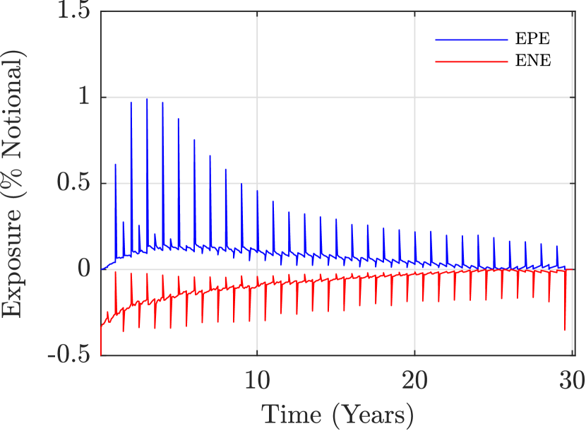
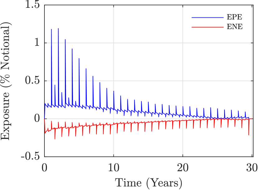
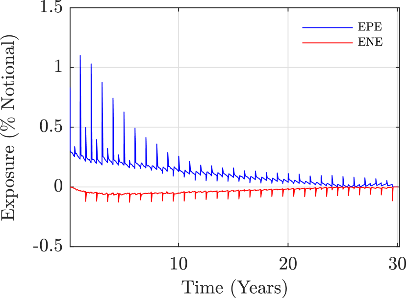
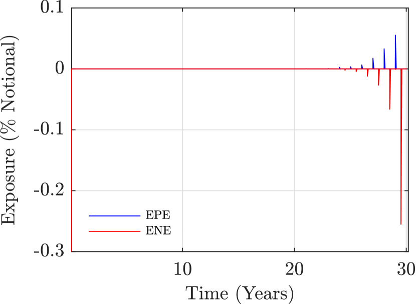
where +(t;ti)superscript𝑡subscript𝑡𝑖\mathcal{H}^{+}(t;t_{i}) is the Expected Positive Exposure (EPE) at time t𝑡t, discretized on interval (ti1,ti]subscript𝑡𝑖1subscript𝑡𝑖(t_{i-1},t_{i}], (t;ti)superscript𝑡subscript𝑡𝑖\mathcal{H}^{-}(t;t_{i}) is the Expected Negative Exposure (ENE), Hm(ti)subscript𝐻𝑚subscript𝑡𝑖H_{m}(t_{i}) is the exposure at time step tisubscript𝑡𝑖t_{i} for path m𝑚m (see eq. 3.1), 𝒮x(t,ti)=1𝒬x(t,ti)subscript𝒮x𝑡subscript𝑡𝑖1subscript𝒬x𝑡subscript𝑡𝑖\mathcal{S}_{\text{x}}(t,t_{i})=1-\mathcal{Q}_{\text{x}}(t,t_{i}) is the survival probability of X at time t𝑡t, referred to time interval [t,ti]𝑡subscript𝑡𝑖[t,t_{i}] and Δ𝒬x(t,ti)=𝒬x(t,ti)𝒬x(t,ti1)Δsubscript𝒬x𝑡subscript𝑡𝑖subscript𝒬x𝑡subscript𝑡𝑖subscript𝒬x𝑡subscript𝑡𝑖1\Delta\mathcal{Q}_{\text{x}}(t,t_{i})=\mathcal{Q}_{\text{x}}(t,t_{i})-\mathcal{Q}_{\text{x}}(t,t_{i-1}) is the marginal default probability of X at time t𝑡t, referred to interval (ti1,ti]subscript𝑡𝑖1subscript𝑡𝑖(t_{i-1},t_{i}].

2.4.3 Analytical Formulas

For some derivatives, such as Swaps, it is possible to analytically solve eqs. 2.29 and 2.30 with considerable benefits in terms of computational time, but limited to uncollateralized case and at trade level. Nevertheless, this approach can be used with the aim to validate the results obtained through a Monte Carlo model (see sec. 5.5).

Starting from eq. 2.29, the CVA of an uncollateralized Swap at time t𝑡t can be written as (see e.g. [16])

CVA(t)=LGDCtT𝔼Q{D(t;u)[Swap(u;T,S,K,ω)]+|t}SB(t,u)𝑑QC(t,u).CVA𝑡𝐿𝐺subscript𝐷Csuperscriptsubscript𝑡𝑇superscript𝔼𝑄conditional-set𝐷𝑡𝑢superscriptdelimited-[]Swap𝑢T,S𝐾𝜔subscript𝑡subscript𝑆B𝑡𝑢differential-dsubscript𝑄C𝑡𝑢\text{CVA}(t)=-LGD_{\text{C}}\int_{t}^{T}\mathbb{E}^{Q}\left\{D(t;u)\left[\text{{Swap}}(u;\text{{T},\text{{S}}},K,\omega)\right]^{+}\left|\mathcal{F}_{t}\right.\right\}S_{\text{B}}(t,u)dQ_{\text{C}}(t,u). (2.34)

By rewriting the price of the Swap in terms of Swap rate (eq. 2.10) and rearranging the terms, the equation above becomes

CVA(t)=LGDCtTN𝔼Q{D(t;u)A(u;S)ω[RxSwap(u;T,S)K]+|t.}SB(t,u)dQC(t,u),=LGDCtTSwaption(t;u,T,S,K,ω)SB(t,u)𝑑QC(t,u),\begin{split}\text{CVA}(t)&=-LGD_{\text{C}}\int_{t}^{T}N\mathbb{E}^{Q}\left\{D(t;u)A(u;\text{{S}})\omega\left[R_{x}^{Swap}(u;\text{{T}},\text{{S}})-K\right]^{+}\big{|}\mathcal{F}_{t}\big{.}\right\}S_{\text{B}}(t,u)dQ_{\text{C}}(t,u),\\ &=-LGD_{\text{C}}\int_{t}^{T}\text{{Swaption}}(t;u,\text{{T}},\text{{S}},K,\omega)S_{\text{B}}(t,u)dQ_{\text{C}}(t,u),\\ \end{split} (2.35)

where Swaption(t;u,T,S,K,ω)Swaption𝑡𝑢TS𝐾𝜔\text{{Swaption}}(t;u,\text{{T}},\text{{S}},K,\omega) denotes the price at time t𝑡t of an European Swaption expiring at time u𝑢u on a Swap having tenor equal to 𝒯=Tu𝒯𝑇𝑢\mathcal{T}=T-u.
Since [A]=[A]+superscriptdelimited-[]𝐴superscriptdelimited-[]𝐴[A]^{-}=[-A]^{+}, the analytical DVA can be obtained as

DVA(t)=LGDBtT𝔼Q{D(t;u)Swap(u;T,S,K,ω)|t.}SC(t,u)dQB(t,u),=LGDBtT𝔼Q{D(t;u)Swap(u;T,S,K,ω)+|t.}SC(t,u)dQB(t,u),=LGDBtTSwaption(t;u,T,S,K,ω)SC(t,u)𝑑QB(t,u).\begin{split}\text{DVA}(t)&=-LGD_{\text{B}}\int_{t}^{T}\mathbb{E}^{Q}\left\{D(t;u)\text{{Swap}}(u;\text{{T},\text{{S}}},K,\omega)^{-}\big{|}\mathcal{F}_{t}\big{.}\right\}S_{\text{C}}(t,u)dQ_{\text{B}}(t,u),\\ &=-LGD_{\text{B}}\int_{t}^{T}\mathbb{E}^{Q}\left\{D(t;u)\text{{Swap}}(u;\text{{T},\text{{S}}},K,-\omega)^{+}\big{|}\mathcal{F}_{t}\big{.}\right\}S_{\text{C}}(t,u)dQ_{\text{B}}(t,u),\\ &=-LGD_{\text{B}}\int_{t}^{T}\text{{Swaption}}(t;u,\text{{T}},\text{{S}},K,-\omega)S_{\text{C}}(t,u)dQ_{\text{B}}(t,u).\\ \end{split} (2.36)

By discretizing the above integrals along a time grid t=t0<t1<<tNT=T𝑡subscript𝑡0subscript𝑡1subscript𝑡subscript𝑁𝑇𝑇t=t_{0}<t_{1}<\ldots<t_{N_{T}}=T, with T𝑇T being the maturity of the Swap one obtains

CVA(t)CVA𝑡\displaystyle\text{CVA}(t) LGDCi=1NTSwaption(t;ti,T,S,K,ω)𝒮B(t,ti)Δ𝒬C(t,ti),absent𝐿𝐺subscript𝐷Csuperscriptsubscript𝑖1subscript𝑁𝑇Swaption𝑡subscript𝑡𝑖TS𝐾𝜔subscript𝒮B𝑡subscript𝑡𝑖Δsubscript𝒬C𝑡subscript𝑡𝑖\displaystyle\cong-LGD_{\text{C}}\sum_{i=1}^{N_{T}}\text{{Swaption}}(t;t_{i},\text{{T}},\text{{S}},K,\omega)\mathcal{S}_{\text{B}}(t,t_{i})\Delta\mathcal{Q}_{\text{C}}(t,t_{i}), (2.37)
DVA(t)DVA𝑡\displaystyle\text{DVA}(t) LGDBi=1NTSwaption(t;ti,T,S,K,ω)𝒮C(t,ti)Δ𝒬B(t,ti).absent𝐿𝐺subscript𝐷Bsuperscriptsubscript𝑖1subscript𝑁𝑇Swaption𝑡subscript𝑡𝑖TS𝐾𝜔subscript𝒮C𝑡subscript𝑡𝑖Δsubscript𝒬B𝑡subscript𝑡𝑖\displaystyle\cong-LGD_{\text{B}}\sum_{i=1}^{N_{T}}\text{{Swaption}}(t;t_{i},\text{{T}},\text{{S}},K,-\omega)\mathcal{S}_{\text{C}}(t,t_{i})\Delta\mathcal{Q}_{\text{B}}(t,t_{i}). (2.38)

Thus, the CVA of a payer (receiver) Swap at time t𝑡t can be written as a weighted sum with weights represented by the values of a strip of co-terminal payer (receiver) European Swaptions expiring at time tisubscript𝑡𝑖t_{i} to enter in a Swap with tenor 𝒯=Tti𝒯𝑇subscript𝑡𝑖\mathcal{T}=T-t_{i}. Symmetrically, DVA can be obtained as a weighted sum over the values of a strip of receiver (payer) European Swaptions.

3 Collateral Modelling

With the aim to reduce the systemic risk posed by non-cleared OTC derivatives, BCBS-IOSCO framework (see [21]) requires institutions engaging in these transactions to post bilaterally Variation Margin (VM) and Initial Margin (IM) on a daily basis at a netting set level. On the one hand, VM aims at covering the current exposure stemming from changes in instrument’s mark to market by reflecting its current size. On the other hand, IM aims at covering the potential future exposure that could arise, in the event of default of the counterparty, from changes in instrument’s mark to market in the the period between last VM exchange and the close-out of the position; this time interval is known as Margin Period of Risk (MPoR).

This section introduces collateral and describes the assumptions made for calculating VM and IM, with a particular focus on ISDA-SIMM dynamic IM.

3.1 Collateral Management

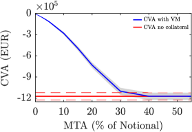
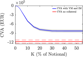
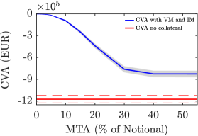
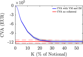
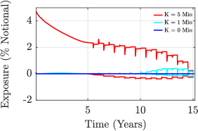
ISDA Master Agreement represents the most common legal framework which governs bilateral OTC derivatives transactions. In particular, the Credit Support Annex (CSA) to ISDA Master Agreement provides the terms under which collateral is posted, along with rules for the resolution of collateral disputes. Certain CSA parameters affect the residual exposure, namely: eligible assets (cash, cash equivalent, government bonds), margin call frequency, threshold (K), defined as the maximum amount of allowed unsecured exposure before any margin call is made, and minimum transfer amount (MTA), defined as the minimum amount that can be transferred for each margin call.

Under perfect collateralization, counterparty risk is suppressed resulting in null CVA/DVA. Theoretically, this corresponds to an ideal CSA ensuring a perfect match between the price V0(t)subscript𝑉0𝑡V_{0}(t) and the corresponding collateral at any time t𝑡t. This condition is approximated in practice with a CSA minimizing any friction between the mark to market and the collateral, i.e. cash collateral in the same currency of the trade, daily margination, flat overnight collateral rate, zero threshold and minimum transfer amount. Nevertheless, real CSA introduces some frictions causing divergences between the price and the corresponding collateral and hence a not negligible counterparty risk. For example, collateral transfers are not instantaneous events and may also takes several days to complete in case of disputes; for this reason, in the event of default, the collateral actually available to the non-defaulting party at the close-out date may differ from the prescribed one.
A simple way to capture these divergences is assuming that VM and IM available at time step tisubscript𝑡𝑖t_{i} depend on the price computed at time tilsubscript𝑡𝑖𝑙t_{i}-l, with l𝑙l being a lag parameter. In this way the time interval [til,ti]subscript𝑡𝑖𝑙subscript𝑡𝑖\left[t_{i}-l,t_{i}\right] represents the MPoR, with tilsubscript𝑡𝑖𝑙t_{i}-l being the last date for which collateral was fully posted and tisubscript𝑡𝑖t_{i} the close-out date. This implies that, while both counterparties stop simultaneously to post collateral for the entire MPoR, contractual cash flows are fully paid. Although simplistic, this assumption can be deemed appropriate in relation to the purposes of our work (advanced models can be found in [40, 27]).
In practical terms, the inclusion of MPoR requires a secondary time grid, built by defining for each tisubscript𝑡𝑖t_{i} of the principal time grid a look-back time point t~i=tilsubscript~𝑡𝑖subscript𝑡𝑖𝑙\tilde{t}_{i}=t_{i}-l such that t~i>t0subscript~𝑡𝑖subscript𝑡0\tilde{t}_{i}>t_{0} at which collateral is computed, with i=1,,NT𝑖1subscript𝑁𝑇i=1,\dots,N_{T}. Formally, from B’s perspective the collateralized exposure Hm(ti)subscript𝐻𝑚subscript𝑡𝑖H_{m}(t_{i}) at time step tisubscript𝑡𝑖t_{i} for a generic path m𝑚m, can be written as

Hm(ti)={[V0,m(ti)VMm(ti;V0,m(t~i),KVM,MTAVM)IMm(ti;V0,m(t~i),KIM,MTAIM)]+ if V0,m(ti)>00 if V0,m(ti)=0[V0,m(ti)VMm(ti;V0,m(t~i),KVM,MTAVM)+IMm(ti;V0,m(t~i),KIM,MTAIM)] if V0,m(ti)<0subscript𝐻𝑚subscript𝑡𝑖casessuperscriptdelimited-[]subscript𝑉0𝑚subscript𝑡𝑖subscriptVM𝑚subscript𝑡𝑖subscript𝑉0𝑚subscript~𝑡𝑖subscriptKVMsubscriptMTAVMsubscriptIM𝑚subscript𝑡𝑖subscript𝑉0𝑚subscript~𝑡𝑖subscriptKIMsubscriptMTAIM if subscript𝑉0𝑚subscript𝑡𝑖00 if subscript𝑉0𝑚subscript𝑡𝑖0superscriptdelimited-[]subscript𝑉0𝑚subscript𝑡𝑖subscriptVM𝑚subscript𝑡𝑖subscript𝑉0𝑚subscript~𝑡𝑖subscriptKVMsubscriptMTAVMsubscriptIM𝑚subscript𝑡𝑖subscript𝑉0𝑚subscript~𝑡𝑖subscriptKIMsubscriptMTAIM if subscript𝑉0𝑚subscript𝑡𝑖0H_{m}(t_{i})=\begin{cases}\left[V_{0,m}\left(t_{i}\right)-\text{VM}_{m}\left(t_{i};V_{0,m}(\tilde{t}_{i}),\text{K}_{\text{VM}},\text{MTA}_{\text{VM}}\right)-\text{IM}_{m}\left(t_{i};V_{0,m}(\tilde{t}_{i}),\text{K}_{\text{IM}},\text{MTA}_{\text{IM}}\right)\right]^{+}&\text{ if }V_{0,m}(t_{i})>0\\ 0&\text{ if }V_{0,m}(t_{i})=0\\ \left[V_{0,m}\left(t_{i}\right)-\text{VM}_{m}\left(t_{i};V_{0,m}(\tilde{t}_{i}),\text{K}_{\text{VM}},\text{MTA}_{\text{VM}}\right)+\text{IM}_{m}\left(t_{i};V_{0,m}(\tilde{t}_{i}),\text{K}_{\text{IM}},\text{MTA}_{\text{IM}}\right)\right]^{-}&\text{ if }V_{0,m}(t_{i})<0\end{cases} (3.1)

Here we assumed that a bilateral and symmetrical CSA is in place, VM is netted, and IM is posted into a segregated account as required by regulation (see [21]); therefore, from B’s perspective VM can be positive (if posted by C) or negative (if posted by B), while IM is always positive.

3.2 Variation Margin

VM modelling is fairly straightforward as it depends on instrument’s mark to market, together with KVMVM{}_{\text{VM}} and MTAVMVM{}_{\text{VM}}. We calculated VM available at time step tisubscript𝑡𝑖t_{i} for a generic path m𝑚m through the following formula

VMm(ti;V0,m(t~i),KVM,MTAVM)=VM^m(t~i1)subscriptVM𝑚subscript𝑡𝑖subscript𝑉0𝑚subscript~𝑡𝑖subscriptKVMsubscriptMTAVMsubscript^VM𝑚subscript~𝑡𝑖1\displaystyle\text{VM}_{m}\left(t_{i};V_{0,m}(\tilde{t}_{i}),\text{K}_{\text{VM}},\text{MTA}_{\text{VM}}\right)=\widehat{\text{VM}}_{m}(\tilde{t}_{i-1})
+𝟙{|(V0,m(t~i)KVM)+VM^m+(t~i1)|>MTAVM}[(V0,m(t~i)KVM)+VM^m+(t~i1)]subscript1superscriptsubscript𝑉0𝑚subscript~𝑡𝑖subscriptKVMsubscriptsuperscript^VM𝑚subscript~𝑡𝑖1subscriptMTAVMdelimited-[]superscriptsubscript𝑉0𝑚subscript~𝑡𝑖subscriptKVMsubscriptsuperscript^VM𝑚subscript~𝑡𝑖1\displaystyle+\mathds{1}_{\left\{\left\lvert\left(V_{0,m}(\tilde{t}_{i})-\text{K}_{\text{VM}}\right)^{+}-\ \widehat{\text{VM}}^{+}_{m}(\tilde{t}_{i-1})\right\rvert>\text{MTA}_{\text{VM}}\right\}}\bigl{[}(V_{0,m}(\tilde{t}_{i})-\text{K}_{\text{VM}})^{+}-\widehat{\text{VM}}^{+}_{m}(\tilde{t}_{i-1})\bigr{]}
+𝟙{|(V0,m(t~i)+KVM)VM^m(t~i1)|>MTAVM}[(V0,m(t~i)+KVM)VM^m(t~i1)],subscript1superscriptsubscript𝑉0𝑚subscript~𝑡𝑖subscriptKVMsubscriptsuperscript^VM𝑚subscript~𝑡𝑖1subscriptMTAVMdelimited-[]superscriptsubscript𝑉0𝑚subscript~𝑡𝑖subscriptKVMsubscriptsuperscript^VM𝑚subscript~𝑡𝑖1\displaystyle+\mathds{1}_{\left\{\left\lvert\left(V_{0,m}(\tilde{t}_{i})+\text{K}_{\text{VM}}\right)^{-}-\ \widehat{\text{VM}}^{-}_{m}(\tilde{t}_{i-1})\right\rvert>\text{MTA}_{\text{VM}}\right\}}\bigl{[}(V_{0,m}(\tilde{t}_{i})+\text{K}_{\text{VM}})^{-}-\widehat{\text{VM}}^{-}_{m}(\tilde{t}_{i-1})\bigr{]}, (3.2)
VM^m(t~i1)=VMm(t~i1)P(t~i1,t~i),subscript^VM𝑚subscript~𝑡𝑖1subscriptVM𝑚subscript~𝑡𝑖1𝑃subscript~𝑡𝑖1subscript~𝑡𝑖\displaystyle\widehat{\text{VM}}_{m}(\tilde{t}_{i-1})=\frac{\text{VM}_{m}(\tilde{t}_{i-1})}{P(\tilde{t}_{i-1},\tilde{t}_{i})}, (3.3)

where VM^m(t~i1)subscript^VM𝑚subscript~𝑡𝑖1\widehat{\text{VM}}_{m}(\tilde{t}_{i-1}) is the value of VM just before its update at t~isubscript~𝑡𝑖\tilde{t}_{i}, and the second and the third terms of eq. 3.2 correspond to the amount of VM posted at time step t~isubscript~𝑡𝑖\tilde{t}_{i} by C and B respectively. In particular, in the second term, C will update VM for the amount exceeding the threshold and VM already in place, provided that this amount is greater than the minimum transfer amount; the same holds for B in case of negative exposure (third term). We imposed null VM for ti=t0subscript𝑡𝑖subscript𝑡0t_{i}=t_{0} and ti=tNTsubscript𝑡𝑖subscript𝑡subscript𝑁𝑇t_{i}=t_{N_{T}}.

3.3 Initial Margin

3.3.1 ISDA Standard Initial Margin Model

In 2013 ISDA, in cooperation with entities first impacted by bilateral margin requirements, started developing the Standard Initial Margin Model (SIMM) with the aim to provide market participant with a uniform risk-sensitive model for calculating bilateral IM (see [23]), preventing both potential disputes between counterparties related to IM determination with different internal models and the overestimation of margin requirements due to the use of the non-risk-sensitive standard approach (see [22]). The first version of the model was published in 2016. On an annual basis model parameters are recalibrated and the methodology is reviewed in order to ensure that regulatory requirements are met. Since our work relies on market data at 28 December 2018, we considered ISDA-SIMM Version 2.1 which was effective from 1 December 2018 to 30 November 2019 (see [41]).

In general, ISDA-SIMM is a parametric VaR model based on Delta, Vega and Curvature (i.e. “pseudo” Gamma) sensitivities, defined across risk factors by asset class, tenor and expiry, computed in line with specific definitions. More in detail, each trade of a portfolio (under a certain CSA agreement) is assigned to a Product Class among Interest Rates & FX, Credit, Equity and Commodity. Since a given trade may have sensitivity to different risk factors, six Risk Classes are defined among Interest Rate, FX, Credit (Qualifying), Credit (non-Qualifying), Equity and Commodity. The margin contributions stemming from the different Risk Classes are combined by means of an aggregation function taking account of Risk Classes correlations. Formally, IM for a generic instrument can be written as

IM =xMx2+xsxψx,sMxMs,absentsubscript𝑥subscriptsuperscriptM2𝑥subscript𝑥subscript𝑠𝑥subscript𝜓𝑥𝑠subscriptM𝑥subscriptM𝑠\displaystyle=\sqrt{\sum_{x}\text{M}^{2}_{x}+\sum_{x}\sum_{s\neq x}\psi_{x,s}\text{M}_{x}\text{M}_{s}}, (3.4)
MxsubscriptM𝑥\displaystyle\text{M}_{x} =DeltaMarginx+VegaMarginx+CurvatureMarginx,absentsubscriptDeltaMargin𝑥subscriptVegaMargin𝑥subscriptCurvatureMargin𝑥\displaystyle=\text{DeltaMargin}_{x}+\text{VegaMargin}_{x}+\text{CurvatureMargin}_{x}, (3.5)

where Mx is the margin component for the Risk Class141414For Credit (Qualifying) Risk Class, which includes instruments whose price is sensitive to correlation between the defaults of different credits within an index or basket (e.g. CDO tranches), an additional margin component, i.e. the BaseCorrMargin shell be calculated (see [41]). x𝑥x, with x{Interest Rate, FX,}𝑥Interest Rate, FX,x\in\left\{\text{Interest Rate, FX,}\dots\right\}, and ψx,ssubscript𝜓𝑥𝑠\psi_{x,s} is the correlation matrix between Risk Classes. IM at portfolio level is obtained by adding together IM contributions from each trade (see [42, 41] for a complete description of the model and underlying assumptions).

In our case, Swaps and European Swaptions are assigned to the Interest Rates & FX Product Class and exposed only to Interest Rate (IR) Risk Class, thus IM=MIRIMsubscriptMIR\text{IM}=\text{M}_{\text{IR}}. Moreover, for a Swap IM=DeltaMarginIRIMsubscriptDeltaMarginIR\text{IM}=\text{DeltaMargin}_{\text{IR}} given the linearity of its payoff. As discussed above, we imposed that collateral available at time step tisubscript𝑡𝑖t_{i} is function of instrument’s value (sensitivities in IM case) at time t~i=tilsubscript~𝑡𝑖subscript𝑡𝑖𝑙\tilde{t}_{i}=t_{i}-l. Therefore, at time step tisubscript𝑡𝑖t_{i} and for a generic path m𝑚m the ISDA-SIMM dynamic IM is given by

IMmSwap(ti)subscriptsuperscriptIMSwap𝑚subscript𝑡𝑖\displaystyle\text{IM}^{\text{Swap}}_{m}(t_{i}) =DeltaMarginIR,m(ti;Vm(t~i)),absentsubscriptDeltaMarginIR𝑚subscript𝑡𝑖subscript𝑉𝑚subscript~𝑡𝑖\displaystyle=\text{DeltaMargin}_{\text{IR},m}\left(t_{i};V_{m}(\tilde{t}_{i})\right), (3.6)
IMmSwpt(ti)subscriptsuperscriptIMSwpt𝑚subscript𝑡𝑖\displaystyle\text{IM}^{\text{Swpt}}_{m}(t_{i}) =DeltaMarginIR,m(ti;Vm(t~i))absentsubscriptDeltaMarginIR𝑚subscript𝑡𝑖subscript𝑉𝑚subscript~𝑡𝑖\displaystyle=\text{DeltaMargin}_{\text{IR},m}\left(t_{i};V_{m}(\tilde{t}_{i})\right)
+VegaMarginIR,m(ti;Vm(t~i))+CurvatureMarginIR,m(ti;Vm(t~i)).subscriptVegaMarginIR𝑚subscript𝑡𝑖subscript𝑉𝑚subscript~𝑡𝑖subscriptCurvatureMarginIR𝑚subscript𝑡𝑖subscript𝑉𝑚subscript~𝑡𝑖\displaystyle+\text{VegaMargin}_{\text{IR},m}\left(t_{i};V_{m}(\tilde{t}_{i})\right)+\text{CurvatureMargin}_{\text{IR},m}\left(t_{i};V_{m}(\tilde{t}_{i})\right). (3.7)

Finally, allowing for KIMIM{}_{\text{IM}} and MTAIMIM{}_{\text{IM}}

IMmp(ti;Vm(t~i),KIM,MTAIM)=𝟙{(IMmp(ti)KIM)+>MTAIM}[(IMmp(ti)KIM)+],p{Swap, Swpt}.formulae-sequencesubscriptsuperscriptIM𝑝𝑚subscript𝑡𝑖subscript𝑉𝑚subscript~𝑡𝑖subscriptKIMsubscriptMTAIMsubscript1superscriptsubscriptsuperscriptIM𝑝𝑚subscript𝑡𝑖subscriptKIMsubscriptMTAIMdelimited-[]superscriptsubscriptsuperscriptIM𝑝𝑚subscript𝑡𝑖subscriptKIM𝑝Swap, Swpt\text{IM}^{p}_{m}\bigl{(}t_{i};V_{m}(\tilde{t}_{i}),\text{K}_{\text{IM}},\text{MTA}_{\text{IM}}\bigr{)}=\mathds{1}_{\left\{\left(\text{IM}^{p}_{m}(t_{i})-\text{K}_{\text{IM}}\right)^{+}>\text{MTA}_{\text{IM}}\right\}}\left[\left(\text{IM}^{p}_{m}(t_{i})-\text{K}_{\text{IM}}\right)^{+}\right],\quad p\in\left\{\text{Swap, Swpt}\right\}. (3.8)

Similar to VM, we imposed null IM for ti=t0subscript𝑡𝑖subscript𝑡0t_{i}=t_{0} and ti=tNTsubscript𝑡𝑖subscript𝑡subscript𝑁𝑇t_{i}=t_{N_{T}}.

3.3.2 Calculation Methodology

The most challenging task underlying ISDA-SIMM dynamic IM is the simulation of forward sensitivities coherently with ISDA definitions, since the subsequent application of weights and aggregation functions is straightforward if we assume that parameters and aggregation rules do not change during the lifetime of the trade. In this section we report the methodology used for computing forward sensitivities, while the other steps to get the different margin components can be found in app. C.

According to ISDA, Delta for the IR Risk Class is defined as price change with respect to a 1 bp shift up in a given tenor151515ISDA defines for both OIS and IBOR curves the following 12 tenors at which Delta shall be computed: 2w, 1m, 3m, 6m, 1y, 2y, 3y, 5y, 10y, 15y, 20y, 30y. of the interest rate curve, expressed in monetary terms. Moreover, ISDA specifies that if computed by the internal system at different tenors, Delta shall be linearly re-allocated onto the SIMM tenors. In general, the price of an instrument which depends on an interest rate curve 𝒞csubscript𝒞𝑐\mathcal{C}_{c} depends explicitly on the zero rates of the curve, which, in turn, depends on the market rates from which the curve is constructed via bootstrapping procedure (see e.g. [36]). Therefore, being Zc=[Z1c,,ZNZc]superscript𝑍𝑐subscriptsuperscript𝑍𝑐1subscriptsuperscript𝑍𝑐subscript𝑁𝑍Z^{c}=[Z^{c}_{1},\dots,Z^{c}_{N_{Z}}] and Rc=[R1c,,RNRc]superscript𝑅𝑐subscriptsuperscript𝑅𝑐1subscriptsuperscript𝑅𝑐subscript𝑁𝑅R^{c}=[R^{c}_{1},\dots,R^{c}_{N_{R}}], respectively, the zero rates and the market rates in correspondence of the term structure of the same curve 𝒞csubscript𝒞𝑐\mathcal{C}_{c}, we calculated the sensitivity with respect to the j𝑗j-th market rate Rjcsubscriptsuperscript𝑅𝑐𝑗R^{c}_{j} at a generic time step tisubscript𝑡𝑖t_{i} as (to ease the notation we neglect subscripts referring to the path)

Δjx(ti)=V(ti)Rjx(ti)subscriptsuperscriptΔ𝑥𝑗subscript𝑡𝑖𝑉subscript𝑡𝑖subscriptsuperscript𝑅𝑥𝑗subscript𝑡𝑖\displaystyle\Delta^{x}_{j}(t_{i})=\frac{\partial V(t_{i})}{\partial R^{x}_{j}(t_{i})} =k=1NZxV(ti)Zkx(ti)Jj,kx,x(t0),absentsubscriptsuperscriptsubscriptsuperscript𝑁𝑥𝑍𝑘1𝑉subscript𝑡𝑖subscriptsuperscript𝑍𝑥𝑘subscript𝑡𝑖subscriptsuperscript𝐽𝑥𝑥𝑗𝑘subscript𝑡0\displaystyle=\sum^{N^{x}_{Z}}_{k=1}\frac{\partial V(t_{i})}{\partial Z^{x}_{k}(t_{i})}J^{x,x}_{j,k}(t_{0}), j=1,,NRx,𝑗1subscriptsuperscript𝑁𝑥𝑅\displaystyle j=1,\dots,N^{x}_{R}, (3.9)
Δjd(ti)=V(ti)Rjd(ti)subscriptsuperscriptΔ𝑑𝑗subscript𝑡𝑖𝑉subscript𝑡𝑖subscriptsuperscript𝑅𝑑𝑗subscript𝑡𝑖\displaystyle\Delta^{d}_{j}(t_{i})=\frac{\partial V(t_{i})}{\partial R^{d}_{j}(t_{i})} =k=1NZdV(ti)Zkd(ti)Jj,kd,d(t0)+k=1NZxV(ti)Zkx(ti)Jj,kx,d(t0),absentsubscriptsuperscriptsubscriptsuperscript𝑁𝑑𝑍𝑘1𝑉subscript𝑡𝑖subscriptsuperscript𝑍𝑑𝑘subscript𝑡𝑖subscriptsuperscript𝐽𝑑𝑑𝑗𝑘subscript𝑡0subscriptsuperscriptsubscriptsuperscript𝑁𝑥𝑍𝑘1𝑉subscript𝑡𝑖subscriptsuperscript𝑍𝑥𝑘subscript𝑡𝑖subscriptsuperscript𝐽𝑥𝑑𝑗𝑘subscript𝑡0\displaystyle=\sum^{N^{d}_{Z}}_{k=1}\frac{\partial V(t_{i})}{\partial Z^{d}_{k}(t_{i})}J^{d,d}_{j,k}(t_{0})+\sum^{N^{x}_{Z}}_{k=1}\frac{\partial V(t_{i})}{\partial Z^{x}_{k}(t_{i})}J^{x,d}_{j,k}(t_{0}), j=1,,NRd,𝑗1subscriptsuperscript𝑁𝑑𝑅\displaystyle j=1,\dots,N^{d}_{R}, (3.10)

where x𝑥x and d𝑑d denote, respectively, the forwarding curve 𝒞xsubscript𝒞𝑥\mathcal{C}_{x} and the discounting curve 𝒞dsubscript𝒞𝑑\mathcal{C}_{d},

Jj,km,n(t0)=Zkm(t0)Rjn(t0),subscriptsuperscript𝐽𝑚𝑛𝑗𝑘subscript𝑡0subscriptsuperscript𝑍𝑚𝑘subscript𝑡0subscriptsuperscript𝑅𝑛𝑗subscript𝑡0J^{m,n}_{j,k}(t_{0})=\frac{\partial Z^{m}_{k}(t_{0})}{\partial R^{n}_{j}(t_{0})}, (3.11)

is an element of the Jacobian matrix (with mn𝑚𝑛m\neq n), assumed to be constant for each ti>t0subscript𝑡𝑖subscript𝑡0t_{i}>t_{0}, and

V(ti)Zkc(ti)V(ti;Zkc(ti)+0.0001)V(ti;Zkc(ti))0.0001,𝑉subscript𝑡𝑖subscriptsuperscript𝑍𝑐𝑘subscript𝑡𝑖𝑉subscript𝑡𝑖subscriptsuperscript𝑍𝑐𝑘subscript𝑡𝑖0.0001𝑉subscript𝑡𝑖subscriptsuperscript𝑍𝑐𝑘subscript𝑡𝑖0.0001\frac{\partial V(t_{i})}{\partial Z^{c}_{k}(t_{i})}\approx\frac{V\bigl{(}t_{i};Z^{c}_{k}(t_{i})+0.0001\bigr{)}-V\bigl{(}t_{i};Z^{c}_{k}(t_{i})\bigr{)}}{0.0001}, (3.12)

is the zero rate Delta sensitivity at tisubscript𝑡𝑖t_{i}. The last term of eq. 3.10 takes into account the indirect Delta sensitivity component of the forwarding zero curve to the discounting zero curve, due to the exogenous nature of the bootstrapping procedure. In line with ISDA prescriptions, for each tenor j𝑗j of the curve 𝒞csubscript𝒞𝑐\mathcal{C}_{c}, we multiplied Delta sensitivity by shock size and linearly allocated this quantity onto the SIMM tenors, obtaining the (1-by-12) Delta vector

Δc(ti)=[Δ2wc(ti),,Δ30yc(ti)].superscriptΔ𝑐subscript𝑡𝑖subscriptsuperscriptΔ𝑐2wsubscript𝑡𝑖subscriptsuperscriptΔ𝑐30ysubscript𝑡𝑖\Delta^{c}(t_{i})=\left[\Delta^{c}_{2\text{w}}(t_{i}),\dots,\Delta^{c}_{30\text{y}}(t_{i})\right]. (3.13)

We then calculated and aggregated the Weighted Sensitivities in order to get Delta Margin (see eqs. C.4 and C.6).

According to ISDA, Vega for the IR Risk Class is defined as price change with respect to a 1% shift up in ATM Black implied volatility σxBlksuperscriptsubscript𝜎𝑥Blk\sigma_{x}^{\text{Blk}}, formally

ν(ti)=V(ti)σxBlk(ti;Te,T,S)V(ti;σxBlk(ti;Te,T,S)+0.01)V(ti;σxBlk(ti;Te,T,S))0.01.𝜈subscript𝑡𝑖𝑉subscript𝑡𝑖superscriptsubscript𝜎𝑥Blksubscript𝑡𝑖subscript𝑇𝑒TS𝑉subscript𝑡𝑖superscriptsubscript𝜎𝑥Blksubscript𝑡𝑖subscript𝑇𝑒TS0.01𝑉subscript𝑡𝑖superscriptsubscript𝜎𝑥Blksubscript𝑡𝑖subscript𝑇𝑒TS0.01\nu(t_{i})=\frac{\partial V(t_{i})}{\partial\sigma_{x}^{\text{Blk}}(t_{i};T_{e},\text{{T}},\text{{S}})}\approx\frac{V\bigl{(}t_{i};\sigma_{x}^{\text{Blk}}(t_{i};T_{e},\text{{T}},\text{{S}})+0.01\bigr{)}-V\bigl{(}t_{i};\sigma_{x}^{\text{Blk}}(t_{i};T_{e},\text{{T}},\text{{S}})\bigr{)}}{0.01}. (3.14)

where we use superscript Blk to distinguish between Black implied volatility σxBlksuperscriptsubscript𝜎𝑥Blk\sigma_{x}^{\text{Blk}} and G2++ parameter σ𝜎\sigma.
Vega sensitivity shall be multiplied by implied volatility to obtain the Vega Risk for expiry Tesubscript𝑇𝑒T_{e} and linearly allocated onto the SIMM expiries, which correspond to the tenors defined for Delta sensitivity. Since G2++ European Swaption pricing formula (see eq. B.12) does not provide for an explicit dependence on Black implied volatility, when performing time simulation Vega cannot be calculated according to the definition above. To overcome this limit we propose the following approximation

V(ti)σxBlk(ti;Te,T,S)V(ti;σ+ϵσ,η+ϵη)V(ti;σ,η)σ^xBlk(ti;Te,T,S)σxBlk(ti;Te,T,S),𝑉subscript𝑡𝑖superscriptsubscript𝜎𝑥Blksubscript𝑡𝑖subscript𝑇𝑒TS𝑉subscript𝑡𝑖𝜎subscriptitalic-ϵ𝜎𝜂subscriptitalic-ϵ𝜂𝑉subscript𝑡𝑖𝜎𝜂superscriptsubscript^𝜎𝑥Blksubscript𝑡𝑖subscript𝑇𝑒TSsuperscriptsubscript𝜎𝑥Blksubscript𝑡𝑖subscript𝑇𝑒TS\frac{\partial V(t_{i})}{\partial\sigma_{x}^{\text{Blk}}(t_{i};T_{e},\text{{T}},\text{{S}})}\approx\frac{V\bigl{(}t_{i};\sigma+\epsilon_{\sigma},\eta+\epsilon_{\eta}\bigr{)}-V\bigl{(}t_{i};\sigma,\eta\bigr{)}}{\hat{\sigma}_{x}^{\text{Blk}}(t_{i};T_{e},\text{{T}},\text{{S}})-\sigma_{x}^{\text{Blk}}(t_{i};T_{e},\text{{T}},\text{{S}})}, (3.15)

where ϵσsubscriptitalic-ϵ𝜎\epsilon_{\sigma} and ϵηsubscriptitalic-ϵ𝜂\epsilon_{\eta} are shocks applied on G2++ model parameters governing the underlying process volatility, and implied volatilities σ^xBlk(ti)superscriptsubscript^𝜎𝑥Blksubscript𝑡𝑖\hat{\sigma}_{x}^{\text{Blk}}(t_{i}) and σxBlk(ti)superscriptsubscript𝜎𝑥Blksubscript𝑡𝑖\sigma_{x}^{\text{Blk}}(t_{i}) are obtained respectively from European Swaption’s prices V(ti;σ+ϵσ,η+ϵη)𝑉subscript𝑡𝑖𝜎subscriptitalic-ϵ𝜎𝜂subscriptitalic-ϵ𝜂V(t_{i};\sigma+\epsilon_{\sigma},\eta+\epsilon_{\eta}) and V(ti;σ,η)𝑉subscript𝑡𝑖𝜎𝜂V(t_{i};\sigma,\eta) by solving the shifted Black pricing formula (see eq. 2.13). In sec. 5.3 we report the analyses conducted to validate this approach and to select the values for the shocks ϵσsubscriptitalic-ϵ𝜎\epsilon_{\sigma}, ϵηsubscriptitalic-ϵ𝜂\epsilon_{\eta} and the Black shift λxsubscript𝜆𝑥\lambda_{x}. In line with ISDA prescriptions, we multiplied Vega sensitivity by implied volatility σxBlksuperscriptsubscript𝜎𝑥Blk\sigma_{x}^{\text{Blk}} and linearly allocated the resulting Vega Risk onto the SIMM expiries, obtaining the (1-by-12) Vega Risk vector

VR(ti)=[VR2w(ti),,VR30y(ti)].VRsubscript𝑡𝑖subscriptVR2wsubscript𝑡𝑖subscriptVR30ysubscript𝑡𝑖\text{VR}(t_{i})=\left[\text{VR}_{2\text{w}}(t_{i}),\dots,\text{VR}_{30\text{y}}(t_{i})\right]. (3.16)

We then calculated and aggregated the Vega Risk Exposures to get Vega Margin (see eqs. C.9 and C.11).

Curvature for the IR Risk Class is calculated by using an approximation of the Vega-Gamma relationship (see [42]). The (1-by-12) Curvature Risk Vector

CVR(ti)=[CVR2w(ti),,CVR30y(ti)]CVRsubscript𝑡𝑖subscriptCVR2wsubscript𝑡𝑖subscriptCVR30ysubscript𝑡𝑖\text{CVR}(t_{i})=\left[\text{CVR}_{2\text{w}}(t_{i}),\dots,\text{CVR}_{30\text{y}}(t_{i})\right] (3.17)

is obtained multiplying the Vega Risk vector by a Scaling Function. We then aggregated the elements of Curvature Risk vector to get Curvature Margin (see eqs. C.14 and C.15).

4 Numerical Simulation

This section reports the results in terms of exposure and CVA/DVA obtained for various interest rate derivatives under three collateralization schemes: without collateral, with VM only and with both VM and IM. In particular, we considered 15 years payer Swaps, 30 years payer Swaps, 5x10 years payer and receiver Forward Swaps, and 5x10 years physically settled European payer and receiver Swaptions with different moneyness levels, listed in tab. 1.

List of analysed instruments
Instrument ω𝜔\omega K𝐾K Moneyness
15Y Swap 1 0.01670.01670.0167 out-of-the-money
1 0.01170.01170.0117 at-the-money
1 0.00670.00670.0067 in-the-money
30Y Swap 1 0.01880.01880.0188 out-of-the-money
1 0.01380.01380.0138 at-the-money
1 0.00880.00880.0088 in-the-money
5x10Y Forward Swap -1 0.01200.01200.0120 out-of-the-money
1 0.01700.01700.0170 at-the-money
1 0.02200.02200.0220 out-of-the-money
5x10Y Swaption -1 0.01200.01200.0120 out-of-the-money
1 0.01700.01700.0170 at-the-money
1 0.02200.02200.0220 out-of-the-money
Table 1: Details on financial instruments analysed. All instruments are denominated in EUR, with N=100𝑁100N=100 Mio, semi-annual floating leg tied to EURIBOR 6M and annual fixed leg. ω=+/1\omega=+/-1 stands for payer/receiver (referred to the fixed leg of the Swap).

4.1 Summary of Numerical Steps

We report below a summary of the numerical steps followed for simulating the exposure and computing CVA/DVA.

  1. 1.

    Discretization of the integrals in eqs. 2.29 and 2.30 along an equally spaced time grid t=t0<<ti<<tNT=T𝑡subscript𝑡0subscript𝑡𝑖subscript𝑡subscript𝑁𝑇𝑇t=t_{0}<\ldots<t_{i}<\dots<t_{N_{T}}=T with granularity Δt=titi1Δ𝑡subscript𝑡𝑖subscript𝑡𝑖1\Delta t=t_{i}-t_{i-1} (see eqs. 2.31 and 2.32). In order to capture all spikes arising in collateralized exposure we added to the time grid a point within the interval (Tj,Tj+l]subscript𝑇𝑗subscript𝑇𝑗𝑙(T_{j},T_{j}+l] for each floating coupon date Tjsubscript𝑇𝑗T_{j} (j=1,,n𝑗1𝑛j=1,\dots,n)161616For the instruments considered, fixed coupon dates are a subset of floating ones since taking place at the same time, otherwise the corresponding coupon dates should have been added to the time grid., with l𝑙l being a lag parameter governing the length of MPoR (see sec. 5.1.2 for details).

  2. 2.

    Construction of a secondary time grid by defining for each time step tisubscript𝑡𝑖t_{i} a look-back time point t~i=tilsubscript~𝑡𝑖subscript𝑡𝑖𝑙\tilde{t}_{i}=t_{i}-l at which compute the collateral actually available at tisubscript𝑡𝑖t_{i} (see sec. 3.1 for details).

  3. 3.

    Calibration of G2++ model parameters p={a,σ,b,η,ρ,Γ1,,Γ14}𝑝𝑎𝜎𝑏𝜂𝜌subscriptΓ1subscriptΓ14p=\left\{a,\sigma,b,\eta,\rho,\Gamma_{1},\dots,\Gamma_{14}\right\} on market ATM European Swaption prices according to the procedure described in sec. 2.3.3.

  4. 4.

    Generation of the pairs (xm(ti)(x_{m}(t_{i}), ym(ti))y_{m}(t_{i})) and (xm(t~i)(x_{m}(\tilde{t}_{i}), ym(t~i))y_{m}(\tilde{t}_{i})) for each time step of both the principal and the secondary time grids and simulated path m=1,,NMC𝑚1subscript𝑁𝑀𝐶m=1,\dots,N_{MC} according to the procedure described in sec. 2.3.4.

  5. 5.

    Calculation of exposure Hm(ti)subscript𝐻𝑚subscript𝑡𝑖H_{m}(t_{i}) for each time step tisubscript𝑡𝑖t_{i} and simulated path m𝑚m according to eq. 3.1. This requires to:

    • a.

      compute instrument’s mark to future V0,m(ti)subscript𝑉0𝑚subscript𝑡𝑖V_{0,m}(t_{i}) at tisubscript𝑡𝑖t_{i} (see pricing formulas in app. B);

    • b.

      compute Variation Margin VMm(ti)subscriptVM𝑚subscript𝑡𝑖\text{VM}_{m}(t_{i}) available at tisubscript𝑡𝑖t_{i}, which is function of instrument’s mark to future V0,m(t~i)subscript𝑉0𝑚subscript~𝑡𝑖V_{0,m}(\tilde{t}_{i}) at t~isubscript~𝑡𝑖\tilde{t}_{i} (see eq. 3.2);

    • c.

      compute ISDA-SIMM dynamic Initial Margin IMm(ti)subscriptIM𝑚subscript𝑡𝑖\text{IM}_{m}(t_{i}) available at tisubscript𝑡𝑖t_{i}, which is function of instrument Delta Δmc(t~i)superscriptsubscriptΔ𝑚𝑐subscript~𝑡𝑖\Delta_{m}^{c}(\tilde{t}_{i}) and Vega νm(t~i)subscript𝜈𝑚subscript~𝑡𝑖\nu_{m}(\tilde{t}_{i}) sensitivities at t~isubscript~𝑡𝑖\tilde{t}_{i} (see eq. 3.8 and sec. 3.3.2 for details on calculation methodology).

  6. 6.

    Calculation of EPE +(t;ti)superscript𝑡subscript𝑡𝑖\mathcal{H}^{+}(t;t_{i}) and ENE (t;ti)superscript𝑡subscript𝑡𝑖\mathcal{H}^{-}(t;t_{i}) for each time step tisubscript𝑡𝑖t_{i} according to eq. 2.33.

  7. 7.

    Calculation of survival probabilities for each time step tisubscript𝑡𝑖t_{i} from default curves built from market CDS quotes through bootstrapping procedure.

  8. 8.

    Calculation of CVA and DVA via eqs. 2.31 and 2.32.

4.2 Model Setup

Aside from G2++ model parameters we can distinguish between calculation parameters and CSA parameters.
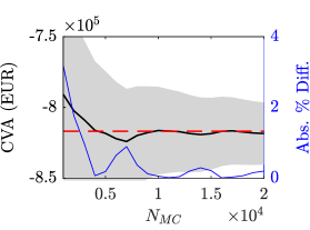
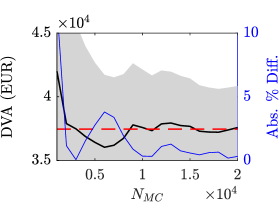
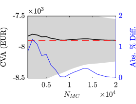
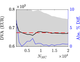
The former affect both the accuracy of the results and the calculation time required and are those related to Monte Carlo approach for calculating CVA/DVA. In particular, we are referring to the granularity of the time grid ΔtΔ𝑡\Delta t used for discretize the integrals, the number of simulated scenarios NMCsubscript𝑁𝑀𝐶N_{MC}, and the parameters used for compute forward Vega sensitivities related to ISDA-SIMM dynamic IM (see eq. 3.15), namely the magnitude of the shocks on G2++ model parameters ϵσsubscriptitalic-ϵ𝜎\epsilon_{\sigma} and ϵηsubscriptitalic-ϵ𝜂\epsilon_{\eta}, and the value of the Black shift λxsubscript𝜆𝑥\lambda_{x} for implied volatility calculation.
CSA parameters affect the residual credit exposure and consequently CVA/DVA with no impacts on the accuracy of the results, and are those related to collateral simulation. In particular, we are referring to threshold K, minimum transfer amount MTA, and to the length of MPoR l𝑙l.

In selecting calculation parameters it is necessary to cope with the trade-off between accuracy and computational effort. The parameterization considered in this section (see tab. 2) is the one that optimizes this trade-off on the basis of specific analyses reported in sec. 5.

Adopted model parameters
Parameters Class Parameter Value
Calculation parameters ΔtΔ𝑡\Delta t 111 month
NMCsubscript𝑁𝑀𝐶N_{MC} 500050005000
ϵσsubscriptitalic-ϵ𝜎\epsilon_{\sigma} 0.010.010.01
ϵηsubscriptitalic-ϵ𝜂\epsilon_{\eta} 0.040.040.04
λxsubscript𝜆𝑥\lambda_{x} 0.060.060.06
CSA parameters l𝑙l 222 days
K 00 EUR
MTA 00 EUR
G2++ parameters a𝑎a 1.1664
σ𝜎\sigma 0.0501
b𝑏b 0.0304
η𝜂\eta 0.0084
ρ𝜌\rho -1.0000
Γ1subscriptΓ1\Gamma_{1} 0.9530
Γ2subscriptΓ2\Gamma_{2} 0.9781
Γ3subscriptΓ3\Gamma_{3} 1.0895
Γ4subscriptΓ4\Gamma_{4} 1.0709
Γ5subscriptΓ5\Gamma_{5} 1.0032
Γ6subscriptΓ6\Gamma_{6} 1.0776
Γ7subscriptΓ7\Gamma_{7} 1.0488
Γ8subscriptΓ8\Gamma_{8} 1.0186
Γ9subscriptΓ9\Gamma_{9} 1.1000
Γ10subscriptΓ10\Gamma_{10} 0.9608
Γ11subscriptΓ11\Gamma_{11} 1.0114
Γ12subscriptΓ12\Gamma_{12} 0.9553
Γ13subscriptΓ13\Gamma_{13} 0.9629
Γ14subscriptΓ14\Gamma_{14} 0.9340
Table 2: Adopted model parameters and respective values. Note that calculation parameters are those optimizing the trade-off between accuracy and calculation time (see sec. 5).
Refer to caption
Figure 1: Calibration errors in absolute percentage terms.

Regarding CSA parameters, in order to get as close as possible to perfect collateralization case, we considered bilateral CSA with K=MTA=0KMTA0\text{K}=\text{MTA}=0 both for VM and IM, with l=2𝑙2l=2 days. In sec. 5.4 the impact of these parameters is assessed. With regard to the calibration of G2++ model parameters, we considered the market ATM European Swaption prices matrix in correspondence of the following expiries ξ𝜉\xi = {2, 3, 4, 5, 6, 7, 8, 9, 10, 12, 15, 20, 25, 30} and tenors 𝔗𝔗\mathfrak{T} = {2, 3, 4, 5, 6, 7, 8, 9, 10, 15, 20, 25, 30}, both expressed in years (see app. A for details). Calibration errors in absolute percentage terms are shown in fig. 1.

4.3 Results

4.3.1 Exposure

The results in terms of EPE and ENE profiles are reported in figs. 2-5 and are aligned on what can be found in the literature (see e.g. [16]).

Focusing on uncollateralized exposures (top panels), the jagged shape observed for the Swaps (figs. 2 and 3) is due to the different coupons frequency (floating coupons received semi-annually, fixed coupons paid annually) which determines semi-annual jumps in instruments’ mark to future at coupon dates. EPE is larger than ENE, in absolute terms, except for the out-of-the-money (OTM) 15 years Swap, due to the forward rates structure which causes expected floating leg values greater than those of the fixed leg. This is evident for in-the-money (ITM) Swaps for which ENE is also almost flat given the low probability to observe negative mark to futures. By comparing the exposures for different maturities, 30 years Swaps are clearly riskier due to the greater number of coupons to be exchanged. The analogous shape for the exposure is observed for the Forward Swaps when coupons payment starts, i.e. from t=5𝑡5t=5 years (fig. 4). Here we can observe the asymmetric effect of forward rates on opposite transactions: the OTM payer Forward Swap displays larger EPE and less negative ENE compared to the OTM receiver one. Physically settled European Swaptions (fig. 5) are written on the same Forward Swaps, before the expiry the exposure is always positive and greater than the one of the corresponding underlying Forward Swap as the price is always positive. After the expiry, OTM paths are excluded as the exercise do not take place, determining smaller EPE and ENE (in absolute value) with respect to the corresponding underlying Forward Swap.

Focusing on exposures with VM (middle panels), a reduction of one order of magnitude can be observed. According to the assumptions made, VM tracks instrument’s mark to future with a delay equal to the length of MPoR (2 days), which represents the only element of friction. This delay causes a material residual exposure characterized by spikes at coupon dates. In general, when only floating coupons are received, one can expect to observe downward spikes due to the fact that the counterparty make a payment for which B still has not returned VM. Conversely, upward spikes arise when fixed cash flows occur and are offset by the downward ones stemming from floating coupons. The magnitude of these spikes is determined by the simulated forward rates structure, e.g. the large upward spikes displayed at the early stage of payer Swaps’ life are due to negative rates (see sec. 5.1.1 for details).

Focusing on exposures with VM and IM (bottom panels), EPE/ENE profiles display spikes with increasing magnitude approaching to maturity, which means that IM turns out to be inadequate to suppress completely the exposure due to its decreasing profile, as displayed in fig. 6.
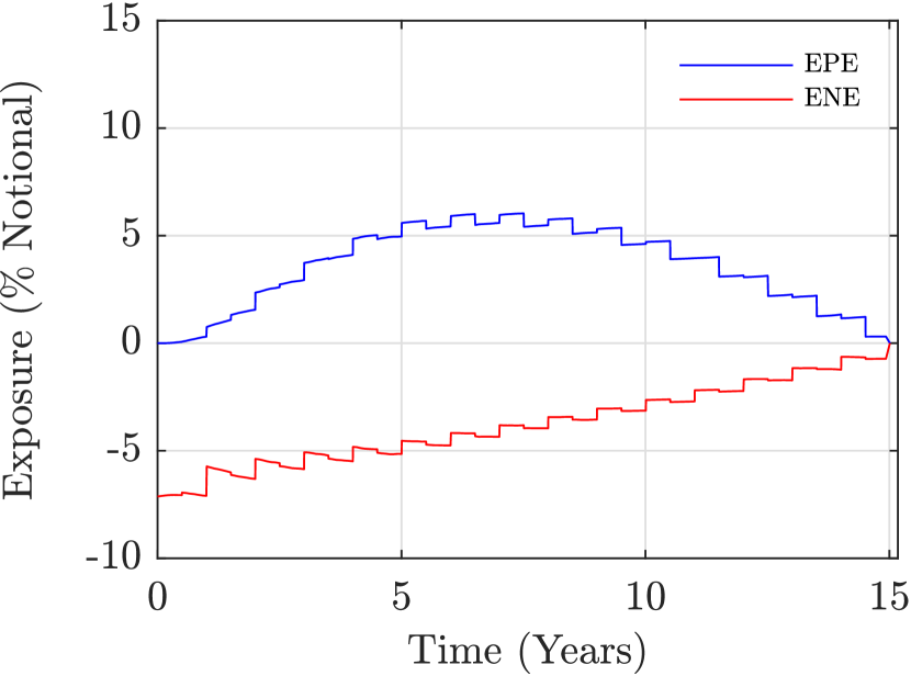
(a) OTM, no collateral.
Refer to caption
(b) ATM, no collateral.
Refer to caption
(c) ITM, no collateral.
Refer to caption
(d) OTM, with VM.
Refer to caption
(e) ATM, with VM.
Refer to caption
(f) ITM, with VM.
Refer to caption
(g) OTM, with VM and IM.
Refer to caption
(h) ATM, with VM and IM.
Refer to caption
(i) ITM, with VM and IM.
Refer to caption
Figure 2: 15 years payer Swaps EUR 100 Mio notional, EPE and ENE profiles (blue and red solid lines respectively) for the collateralization schemes (top: no collateral, mid: VM, bottom: VM and IM) and moneyness (left: OTM, mid: ATM, right: ITM) considered. To enhance plots readability, we excluded collateralized EPE/ENE for time step t0subscript𝑡0t_{0} as not mitigated by collateral. Model setup as in tab. 2. Quantities expressed as a percentage of the notional.
(a) OTM, no collateral.
Refer to caption
(b) ATM, no collateral.
Refer to caption
(c) ITM, no collateral.
Refer to caption
(d) OTM, with VM.
Refer to caption
(e) ATM, with VM.
Refer to caption
(f) ITM, with VM.
Refer to caption
(g) OTM, with VM and IM.
Refer to caption
(h) ATM, with VM and IM.
Refer to caption
(i) ITM, with VM and IM.
Refer to caption
Figure 3: 30 years payer Swaps EUR 100 Mio notional, EPE and ENE profiles (blue and red solid lines respectively) for the collateralization schemes (top: no collateral, mid: VM, bottom: VM and IM) and moneyness (left: OTM, mid: ATM, right: ITM) considered. To enhance plots readability, we excluded collateralized EPE/ENE for time step t0subscript𝑡0t_{0} as not mitigated by collateral. Model setup as in tab. 2. Quantities expressed as a percentage of the notional.
(a) Receiver OTM, no collat.
Refer to caption
(b) Payer ATM, no collat.
Refer to caption
(c) Payer OTM, no collat.
Refer to caption
(d) Receiver OTM, with VM.
Refer to caption
(e) Payer ATM, with VM.
Refer to caption
(f) Payer OTM, with VM.
Refer to caption
(g) Receiver OTM, with VM and IM.
Refer to caption
(h) Payer ATM, with VM and IM.
Refer to caption
(i) Payer OTM, with VM and IM.
Refer to caption
Figure 4: 5x10 years Forward Swaps EUR 100 Mio notional, EPE and ENE profiles (blue and red solid lines respectively) for the collateralization schemes (top: no collateral, mid: VM, bottom: VM and IM) and moneyness (left: reicever OTM, mid: payer ATM, right: payer OTM) considered. To enhance plots readability, we excluded collateralized EPE/ENE for time step t0subscript𝑡0t_{0} as not mitigated by collateral. Model setup as in tab. 2. Quantities expressed as a percentage of the notional.
(a) Receiver OTM, no collat.
Refer to caption
(b) Payer ATM, no collat.
Refer to caption
(c) Payer OTM, no collat.
Refer to caption
(d) Receiver OTM, with VM.
Refer to caption
(e) Payer ATM, with VM.
Refer to caption
(f) Payer OTM, with VM.
Refer to caption
(g) Receiver OTM, with VM and IM.
Refer to caption
(h) Payer ATM, with VM and IM.
Refer to caption
(i) Payer OTM, with VM and IM.
Refer to caption
Figure 5: 5x10 years physically settled European Swaptions EUR 100 Mio notional, EPE and ENE profiles (blue and red solid lines respectively) for the collateralization schemes (top: no collateral, mid: VM, bottom: VM and IM) and moneyness (left: reicever OTM, mid: payer ATM, right: payer OTM) considered. To enhance plots readability, we excluded collateralized EPE/ENE for time step t0subscript𝑡0t_{0} as not mitigated by collateral. Model setup as in tab. 2. Quantities expressed as a percentage of the notional.
(a) 15Y Swap OTM.
Refer to caption
(b) 15Y Swap ATM.
Refer to caption
(c) 15Y Swap ITM.
Refer to caption
(d) 30Y Swap OTM.
Refer to caption
(e) 30Y Swap ATM.
Refer to caption
(f) 30Y Swap ITM
Refer to caption
(g) 5x10Y R Fwd Swap OTM.
Refer to caption
(h) 5x10Y P Fwd Swap ATM.
Refer to caption
(i) 5x10Y P Fwd Swap OTM.
Refer to caption
(j) 5x10Y R Swaption OTM.
Refer to caption
(k) 5x10Y P Swaption ATM.
Refer to caption
(l) 5x10Y P Swaption OTM.
Refer to caption
Figure 6: Average values for VM (blue lines, right-hand scale) and IM (black lines, left-hand scale) for instruments in tab. 1. Letter P and R distinguish between payer and receiver instruments where necessary. Model setup as in tab. 2. Quantities expressed as a percentage of the notional.

4.3.2 XVA

The results in terms of CVA/DVA reported in tab. 3 are driven by the elements above discussed.

CVA and DVA for the instruments in tab. 1
Collateral Instrument Moneyness ω𝜔\omega CVA DVA
None 15Y Swap OTM 1 779 085-779085-779\,085 (±plus-or-minus\pm 666%) 884 382884382884\,382 (±plus-or-minus\pm 666%)
15Y Swap ATM 1 1 172 938-1172938-1\,172\,938 (±plus-or-minus\pm 444%) 475 324475324475\,324 (±plus-or-minus\pm 999%)
15Y Swap ITM 1 1 681 190-1681190-1\,681\,190 (±plus-or-minus\pm 444%) 240 662240662240\,662 (±plus-or-minus\pm 121212%)
30Y Swap OTM 1 2 630 312-2630312-2\,630\,312 (±plus-or-minus\pm 555%) 2 218 07122180712\,218\,071 (±plus-or-minus\pm 777%)
30Y Swap ATM 1 3 756 886-3756886-3\,756\,886 (±plus-or-minus\pm 444%) 1 233 12912331291\,233\,129 (±plus-or-minus\pm 101010%)
30Y Swap ITM 1 5 173 086-5173086-5\,173\,086 (±plus-or-minus\pm 333%) 650 447650447650\,447 (±plus-or-minus\pm 141414%)
5x10Y Fwd Swap OTM -1 387 131-387131-387\,131 (±plus-or-minus\pm 999%) 1 373 95113739511\,373\,951 (±plus-or-minus\pm 444%)
5x10Y Fwd Swap ATM 1 821 210-821210-821\,210 (±plus-or-minus\pm 555%) 714 338714338714\,338 (±plus-or-minus\pm 777%)
5x10Y Fwd Swap OTM 1 530 527-530527-530\,527 (±plus-or-minus\pm 777%) 1 134 27311342731\,134\,273 (±plus-or-minus\pm 555%)
5x10Y Swaption OTM -1 390 339-390339-390\,339 (±plus-or-minus\pm 999%) 43 0114301143\,011 (±plus-or-minus\pm 171717%)
5x10Y Swaption ATM 1 818 308-818308-818\,308 (±plus-or-minus\pm 555%) 36 4183641836\,418 (±plus-or-minus\pm 171717%)
5x10Y Swaption OTM 1 519 394-519394-519\,394 (±plus-or-minus\pm 777%) 34 8253482534\,825 (±plus-or-minus\pm 181818%)
VM 15Y Swap OTM 1 6506-6506-6506 (±plus-or-minus\pm 999%) 10 3841038410\,384 (±plus-or-minus\pm 999%)
15Y Swap ATM 1 8856-8856-8856 (±plus-or-minus\pm 888%) 681468146814 (±plus-or-minus\pm 121212%)
15Y Swap ITM 1 10 787-10787-10\,787 (±plus-or-minus\pm 777%) 347934793479 (±plus-or-minus\pm 171717%)
30Y Swap OTM 1 23 462-23462-23\,462 (±plus-or-minus\pm 999%) 32 1853218532\,185 (±plus-or-minus\pm 101010%)
30Y Swap ATM 1 30 123-30123-30\,123 (±plus-or-minus\pm 888%) 21 3162131621\,316 (±plus-or-minus\pm 131313%)
30Y Swap ITM 1 35 292-35292-35\,292 (±plus-or-minus\pm 777%) 11 6951169511\,695 (±plus-or-minus\pm 181818%)
5x10Y Fwd Swap OTM -1 5130-5130-5130 (±plus-or-minus\pm 131313%) 13 9751397513\,975 (±plus-or-minus\pm 888%)
5x10Y Fwd Swap ATM 1 8322-8322-8322 (±plus-or-minus\pm 999%) 986298629862 (±plus-or-minus\pm 101010%)
5x10Y Fwd Swap OTM 1 5899-5899-5899 (±plus-or-minus\pm 111111%) 13 4581345813\,458 (±plus-or-minus\pm 888%)
5x10Y Swaption OTM -1 4969-4969-4969 (±plus-or-minus\pm 121212%) 633633633 (±plus-or-minus\pm 242424%)
5x10Y Swaption ATM 1 7831-7831-7831 (±plus-or-minus\pm 999%) 665665665 (±plus-or-minus\pm 232323%)
5x10Y Swaption OTM 1 5744-5744-5744 (±plus-or-minus\pm 101010%) 624624624 (±plus-or-minus\pm 242424%)
VM and IM 15Y Swap OTM 1 7-7-7 (±plus-or-minus\pm 242424%) 121212 (±plus-or-minus\pm 141414%)
15Y Swap ATM 1 4-4-4 (±plus-or-minus\pm 323232%) 777 (±plus-or-minus\pm 202020%)
15Y Swap ITM 1 2-2-2 (±plus-or-minus\pm 434343%) 444 (±plus-or-minus\pm 303030%)
30Y Swap OTM 1 2-2-2 (±plus-or-minus\pm 202020%) 444 (±plus-or-minus\pm 111111%)
30Y Swap ATM 1 1-1-1 (±plus-or-minus\pm 272727%) 222 (±plus-or-minus\pm 151515%)
30Y Swap ITM 1 1-1-1 (±plus-or-minus\pm 373737%) 111 (±plus-or-minus\pm 222222%)
5x10Y Fwd Swap OTM -1 7-7-7 (±plus-or-minus\pm 191919%) 444 (±plus-or-minus\pm 313131%)
5x10Y Fwd Swap ATM 1 7-7-7 (±plus-or-minus\pm 232323%) 131313 (±plus-or-minus\pm 141414%)
5x10Y Fwd Swap OTM 1 12-12-12 (±plus-or-minus\pm 202020%) 202020 (±plus-or-minus\pm 111111%)
5x10Y Swaption OTM -1 12-12-12 (±plus-or-minus\pm 282828%) 777 (±plus-or-minus\pm 505050%)
5x10Y Swaption ATM 1 13-13-13 (±plus-or-minus\pm 303030%) 383838 (±plus-or-minus\pm 171717%)
5x10Y Swaption OTM 1 17-17-17 (±plus-or-minus\pm 303030%) 464646 (±plus-or-minus\pm 161616%)
Table 3: CVA and DVA for instruments in tab. 1 for the three collateralization schemes considered, 3σ𝜎\sigma confidence intervals in parentheses. Model setup as in tab. 2. Quantities expressed in EUR.

Focusing on uncollateralized CVA/DVA, Swaps display larger CVA (DVA) figures for ITM (OTM) instruments due to the greater probability to observe positive (negative) mark to futures, also reflected in lower Monte Carlo errors. Moreover, CVA is larger than DVA except for the OTM 15 years Swap due to the simulated forward rates structure discussed above. Finally, analysing the results for different maturities, the higher risk of 30 years Swaps leads to larger adjustments compared to those maturing in 15 years. Analogous results are obtained for Forward Swaps. In this case, the asymmetric effect of simulated forward rates on opposite transactions causes larger CVA and smaller DVA for the OTM payer Forward Swap with respect to the OTM receiver one. Slightly lower (absolute) CVA values are observed for the corresponding physically settled European Swaptions since OTM paths are excluded after the exercise, while DVA values are considerably lower as negative exposure exists only after the expiry.

Focusing on CVA/DVA with VM only, the results show that the adjustments are reduced on average by approx. two orders of magnitude. In this case CVA/DVA are widely driven by spikes in exposure profiles which determine changes in certain relations previously identified. In particular, the 30 years OTM Swap displays greater DVA compared to CVA since ENE is larger than EPE between the spikes and their magnitude becomes larger for ENE by approaching the maturity (where default probability increases). The same can be observed for the 5x10 years ATM Forward Swap.

Focusing on CVA/DVA with VM and IM, the results show that the adjustments are reduced on average by approx. four orders of magnitude with respect to uncollateralized case. CVA/DVA are entirely due to the spikes closest to maturity which are not fully suppressed by IM. Largest DVA compared to CVA are observed for payer instruments for which wide spikes are observed in ENE as the difference between fixed rate and floating rate are greater. For the same reason receiver instruments display larger CVA figures.

5 Model Validation

Previous sections suggest that the numerical calculation of CVA/DVA requires various assumptions for modelling and computing the relevant quantities. Since affecting the stability of the results, these assumptions are source of model risk to be properly addressed.
The purpose of this section is twofold: on the one hand, we want to validate the framework adopted in sec. 4 by assessing its robustness and selecting a parameterization which optimizes the trade-off between accuracy and performance, on the other hand, we want to identify the most significant sources of model risk involved in exposure modelling and hence CVA/DVA calculation. To ease the presentation we report the results only for a subset of the instruments in tab. 1, mainly the 15 years ATM payer Swap and the 5x10 years ATM physically settled European payer Swaption. Analogous results are obtained for the other instruments.

5.1 Time Grid Construction

The numerical solution of eqs. 2.29 and 2.30 involves the discretization of the integral along a grid of valuation dates in correspondence of which the exposure is computed. In selecting the length of time steps ΔtΔ𝑡\Delta t it is necessary to optimize the trade-off between precision and computational effort. In fact, an high granularity reduces the discretization error but makes the calculation unfeasible due to long time required. Furthermore, the inclusion in the model of the MPoR requires to discretize the aforementioned equations in such a way to capture all periodical spikes in Swap’s collateralized exposure which have material impact on CVA/DVA.
In this section we first analyse the nature of spikes in collateralized exposure when a daily grid is used and their impact on CVA/DVA. We then propose a possible workaround which allows to capture all spikes at lower granularities, at the end we report the results of a convergence analysis aimed at finding a granularity which ensures a good compromise between precision and computational time.

5.1.1 Spikes Analysis

Spikes arising in collateralized exposure are due to the MPoR since it implies that the collateral available at time step tisubscript𝑡𝑖t_{i} depends on instrument’s mark to future at time step t~i=tilsubscript~𝑡𝑖subscript𝑡𝑖𝑙\tilde{t}_{i}=t_{i}-l, assumed to be the last date for which VM and IM were fully posted (see sec. 3.1). The granularity of the time grid used to discretize the integrals in eqs. 2.29 and 2.30 determines the existence of spikes in collateralized exposure profile, in fact a time grid with daily granularity is able to capture all spikes as shown in fig. 7, which displays EPE/ENE profiles for the 15 years ATM payer Swap (left-hand side panel) and the 5x10 years ATM physically settled European payer Swaption (right-hand side panel) for the three collateralization schemes considered.

(a) EPE and ENE Swap no collateral.
Refer to caption
(b) EPE and ENE Swaption no collateral.
Refer to caption
(c) EPE and ENE Swap with VM.
Refer to caption
(d) EPE and ENE Swaption with VM.
Refer to caption
(e) EPE and ENE Swap with VM and IM.
Refer to caption
(f) EPE and ENE Swaption with VM and IM.
Refer to caption
Figure 7: 15 years ATM payer Swap (left-hand side) and 5x10 years ATM physically settled European payer Swaption (right-hand side) EUR 100 Mio notional, EPE and ENE profiles (blue solid lines) on a daily grid for the three collateralization schemes considered (top: no collateral, mid: VM, bottom: VM and IM). Black crosses correspond to floating leg coupon dates (semiannual frequency), red circles correspond to fixed coupon dates (annual frequency), green triangles correspond to Swaption’s expiry. Spikes in collateralized exposure at inception and at coupon dates are an effect of MPoR. To enhance Swaption’s plots readability, we excluded collateralized EPE for time steps t0subscript𝑡0t_{0} and t1subscript𝑡1t_{1} as not mitigated by collateral (mid and bottom right-hand panels), in particular EPE(t0subscript𝑡0t_{0}) corresponds to Swaption’s price 5 030 423 EUR (approx. 5%percent55\% of the notional). Other model parameters as in tab. 2. Quantities expressed as a percentage of the notional.

As can be seen, when only VM is considered, spikes emerge at inception as no collateral is posted, and at coupon dates as sudden changes in mark to future are captured by VM with a delay due to MPoR. When also IM is considered, spikes closest to maturity persist due to the downward profile of IM.

We further investigated the nature of these spikes by focusing on the 15 years ATM payer Swap’s Expected Exposure (EE)171717The Expected Exposure (EE) is defined as: (t,ti)=P(t;ti)1NMCm=1NMCHm(ti)𝑡subscript𝑡𝑖𝑃𝑡subscript𝑡𝑖1subscript𝑁𝑀𝐶superscriptsubscript𝑚1subscript𝑁𝑀𝐶subscript𝐻𝑚subscript𝑡𝑖\mathcal{H}(t,t_{i})=P(t;t_{i})\frac{1}{N_{MC}}\sum_{m=1}^{N_{MC}}H_{m}(t_{i}). without collateral and with VM, displayed in fig. 8.

(a) EE no collateral and Swap legs.
Refer to caption
(b) Jump in EE no collateral.
Refer to caption
(c) EE with VM and Swap legs.
Refer to caption
(d) Spike in EE with VM.
Refer to caption
Figure 8: 15 years ATM payer Swap EUR 100 Mio notional, analysis on spikes in EE with VM. Top left-hand side panel displays floating and fixed legs average values (black and red solid lines respectively, black crosses: floating coupon dates, red circles: fixed coupon dates, left-hand scale) and uncollateralized EE (blue solid line, right-hand scale), which is positive since floating leg is always greater than fixed leg. Bottom left-hand side panel displays EE with VM (blue solid line, right-hand scale). Top right-hand side panel displays the jump in uncollateralized EE (blue solid line, right-hand scale) right after fixed and floating coupons payment taking place at t=𝑡absentt= 1y2d, and given by a simultaneous increase in floating leg and drop in fixed one (black and red solid lines respectively, left-hand scale). Bottom right-hand side panel displays the spike in EE with VM (blue dotted line) occurring right after fixed and floating coupons payment due to the fact that VM (cyan dashed line) captures the jump in uncollateralized EE (blue solid line) with a delay equal to the length of the MPoR. Daily grid considered, other model parameters as in tab. 2. Quantities expressed as a percentage of the notional.

Left-hand side panels show that both the jagged shape of uncollalteralized EE (fig. 8(a)) and the spikes in EE with VM (fig. 8(b)) are determined by sudden changes in the average values of Swap legs right after coupon payments. Right-hand side panels show a focus around t=1𝑡1t=1y, when both fixed and floating coupons take place: after these cash flows, the average value of floating leg increases and fixed leg one decreases, resulting in a positive jump in uncollateralized EE at t=𝑡absentt= 1y3d (fig. 8(c)). This jump is captured by VM at t=𝑡absentt= 1y5d, this delay of 2 days due to MPoR causes an upward spike in EE with VM (fig. 8(d)). The direction and magnitude depend on the simulated forward rates structure and on whether fixed or floating coupon payments take place.
Focusing on semiannual floating coupons paid by C, two different behaviours can be observed during the lifetime of the Swap. The first three floating coupons determine positive jumps in uncollateralized EE and upward spikes in EE with VM. This is due to the fact that the simulated forward rates are on average negative until 2.5 years implying that, until that time, these coupons are actually paid by B. Once forward rates revert to positive values, negative jumps in uncollateralized EE and downward spikes in EE with VM arise in correspondence of the remaining floating coupons (figs. 8(a) and 8(b)).
When also annual fixed coupons paid by B take place, positive jumps in uncollateralized EE and upward spikes with decreasing magnitude in EE with VM can be observed. Negative rates cause wide spikes in correspondence of the first two fixed and floating coupons due to the simultaneous increase in the average value of floating leg and decrease in the fixed leg one, in B’s perspective, right after coupons payment (figs. 8(c) and 8(d)).

The impact of spikes on total CVA and DVA is significant: with only VM the contribution is respectively of 7%percent77\% and 4%percent44\% for the 15 years ATM payer Swap and of 2%percent22\% and 16%percent1616\% for the 5x10 years ATM physically settled European payer Swaption. With also IM the exposure between spikes is suppressed, therefore CVA and DVA are completely attributable to spikes.

5.1.2 Parsimonious Time Grid

Although a daily grid represents the best discrete approximation of the integrals in eqs. 2.29 and 2.30, it is very limited in terms of computational time required, as can be seen from the last column of tab. 4. The most time consuming component is represented by IM which involves the calculation of several forward sensitivities for each path (see sec. 3.3.2). Computational time lengthens further for Swaptions due to the numerical resolution of G2++ pricing formula (see eq. B.12). The calculation of CVA/DVA using a daily grid is clearly unfeasible, this forced us to consider a lower granularity.

A standard less granular evenly spaced time grid may produce biased CVA/DVA values if not capable of capturing all spikes in collateralized exposure. In fact, the spike due to the coupon occurring at time Tjsubscript𝑇𝑗T_{j} would emerge only if the time grid includes a point tisubscript𝑡𝑖t_{i} falling within the interval (Tj,Tj+l]subscript𝑇𝑗subscript𝑇𝑗𝑙(T_{j},T_{j}+l]. A possible workaround to make sure to capture all spikes could be to add to a standard time grid the set of points {Tj+1d}j=1nsuperscriptsubscriptsubscript𝑇𝑗1d𝑗1𝑛\{T_{j}+1\text{d}\}_{j=1}^{n}, where Tjsubscript𝑇𝑗T_{j} is the j𝑗j-th floating coupon date and n𝑛n is the number of floating coupons181818For the instruments considered, fixed coupon dates are a subset of floating ones since taking place at the same time, otherwise the corresponding coupon dates should have been added to the time grid.; we will refer to this augmented grid as the joint grid. The comparison between EPE/ENE for the 15 years ATM payer Swap, obtained through standard and joint grids with monthly granularity for the three collateralization schemes considered, is shown in fig. 9. The 5x10 years ATM physically settled European payer Swaption displays same results and is not reported.

(a) Standard grid EPE and ENE no collateral.
Refer to caption
(b) Joint grid EPE and ENE no collateral.
Refer to caption
(c) Standard grid EPE and ENE with VM.
Refer to caption
(d) Joint grid EPE and ENE with VM.
Refer to caption
(e) Standard grid EPE and ENE with VM and IM.
Refer to caption
(f) Joint grid EPE and ENE with VM and IM.
Refer to caption
Figure 9: 15 years ATM payer Swap EUR 100 Mio notional, comparison between EPE and ENE profiles obtained with standard grid (left-hand side) and joint grid (right-hand side) with monthly granularity for the three collateralization schemes considered (top: no collateral, mid: VM, bottom: VM and IM). The graphs show that it is possible to capture spikes in collateralized exposure by adding to the standard grid the set of time points {Tj+1d}j=1nsuperscriptsubscriptsubscript𝑇𝑗1d𝑗1𝑛\{T_{j}+1\text{d}\}_{j=1}^{n}, where Tjsubscript𝑇𝑗T_{j} is the j𝑗j-th floating coupon date and n𝑛n is the number of floating coupons. Other model parameters as in tab. 2. Quantities expressed as a percentage of the notional.

As can be seen, uncollateralized exposure is similar for both grids, while standard grid fails to capture spikes in collateralized exposure since no time point within the interval (Tj,Tj+l]subscript𝑇𝑗subscript𝑇𝑗𝑙(T_{j},T_{j}+l] is included for each coupon date Tjsubscript𝑇𝑗T_{j}. Moreover, with no spikes, IM suppresses completely the residual exposure resulting in null CVA/DVA. Instead, all spikes are captured by the joint grid which allows to correctly model the collateralized exposure with considerable time-saving benefits.

With the aim to optimize the trade-off between precision and computation time, we investigated CVA/DVA convergence with respect to different granularities for the joint grid, setting the results obtained with the daily grid as benchmark. In particular, we considered monthly, quarterly, semiannual and annual time steps. The results for the 15 years ATM payer Swap and the 5x10 years ATM physically settled European payer Swaption, for the three collateralization schemes considered are reported in tab. 4.

CVA and DVA convergence with respect to time grid granularity
Instrument Collateral ΔtΔ𝑡\Delta t CVA DVA Time (min)
12M 1 119 629-1119629-1\,119\,629 (±plus-or-minus\pm 444%) 485 660485660485\,660 (±plus-or-minus\pm 888%) 0.450.450.45
6M 1 170 271-1170271-1\,170\,271 (±plus-or-minus\pm 444%) 478 016478016478\,016 (±plus-or-minus\pm 999%) 0.600.600.60
None 3M 1 172 139-1172139-1\,172\,139 (±plus-or-minus\pm 444%) 476 789476789476\,789 (±plus-or-minus\pm 999%) 0.900.900.90
1M 1 172 938-1172938-1\,172\,938 (±plus-or-minus\pm 444%) 475 324475324475\,324 (±plus-or-minus\pm 999%) 2.102.102.10
1D 1 173 296-1173296-1\,173\,296 (±plus-or-minus\pm 444%) 474 469474469474\,469 (±plus-or-minus\pm 999%) 54.8054.8054.80
12M 13 894-13894-13\,894 (±plus-or-minus\pm 101010%) 22 4522245222\,452 (±plus-or-minus\pm 111111%) 0.900.900.90
6M 7025-7025-7025 (±plus-or-minus\pm 888%) 559755975597 (±plus-or-minus\pm 121212%) 1.201.201.20
Swap VM 3M 8138-8138-8138 (±plus-or-minus\pm 888%) 633863386338 (±plus-or-minus\pm 121212%) 1.801.801.80
1M 8856-8856-8856 (±plus-or-minus\pm 888%) 681468146814 (±plus-or-minus\pm 121212%) 4.204.204.20
1D 9374-9374-9374 (±plus-or-minus\pm 888%) 711871187118 (±plus-or-minus\pm 121212%) 109.60109.60109.60
12M 16-16-16 (±plus-or-minus\pm 939393%) 109810981098 (±plus-or-minus\pm 171717%) 12.3812.3812.38
6M 4-4-4 (±plus-or-minus\pm 323232%) 777 (±plus-or-minus\pm 202020%) 16.5016.5016.50
VM and IM 3M 4-4-4 (±plus-or-minus\pm 323232%) 777 (±plus-or-minus\pm 202020%) 24.7524.7524.75
1M 4-4-4 (±plus-or-minus\pm 323232%) 777 (±plus-or-minus\pm 202020%) 57.7557.7557.75
1D 6-6-6 (±plus-or-minus\pm 272727%) 161616 (±plus-or-minus\pm 151515%) 1507.011507.011507.01
12M 775 964-775964-775\,964 (±plus-or-minus\pm 666%) 41 3574135741\,357 (±plus-or-minus\pm 161616%) 4.324.324.32
6M 815 745-815745-815\,745 (±plus-or-minus\pm 555%) 36 7053670536\,705 (±plus-or-minus\pm 171717%) 6.076.076.07
None 3M 817 396-817396-817\,396 (±plus-or-minus\pm 555%) 36 5443654436\,544 (±plus-or-minus\pm 171717%) 9.759.759.75
1M 818 308-818308-818\,308 (±plus-or-minus\pm 555%) 36 4183641836\,418 (±plus-or-minus\pm 171717%) 23.5723.5723.57
1D 819 616-819616-819\,616 (±plus-or-minus\pm 555%) 36 3673636736\,367 (±plus-or-minus\pm 171717%) 640.03640.03640.03
12M 6933-6933-6933 (±plus-or-minus\pm 111111%) 736373637363 (±plus-or-minus\pm 161616%) 8.028.028.02
6M 6940-6940-6940 (±plus-or-minus\pm 999%) 638638638 (±plus-or-minus\pm 222222%) 11.2711.2711.27
Swaption VM 3M 7481-7481-7481 (±plus-or-minus\pm 999%) 649649649 (±plus-or-minus\pm 232323%) 17.7717.7717.77
1M 7831-7831-7831 (±plus-or-minus\pm 999%) 665665665 (±plus-or-minus\pm 232323%) 43.7743.7743.77
1D 7734-7734-7734 (±plus-or-minus\pm 999%) 527527527 (±plus-or-minus\pm 252525%) 1188.631188.631188.63
12M 16-16-16 (±plus-or-minus\pm 666666%) 110211021102 (±plus-or-minus\pm 181818%) 119.63119.63119.63
6M 13-13-13 (±plus-or-minus\pm 303030%) 383838 (±plus-or-minus\pm 171717%) 168.13168.13168.13
VM and IM 3M 13-13-13 (±plus-or-minus\pm 303030%) 383838 (±plus-or-minus\pm 171717%) 265.13265.13265.13
1M 13-13-13 (±plus-or-minus\pm 303030%) 383838 (±plus-or-minus\pm 171717%) 653.15653.15653.15
1D 38-38-38 (±plus-or-minus\pm 333%) 121212 (±plus-or-minus\pm 191919%) 17 738.0717738.0717\,738.07
Table 4: 15 years ATM payer Swap and 5x10 years ATM physically settled European payer Swaption EUR 100 Mio notional, CVA and DVA convergence with respect to joint grid granularity for the three collateralization schemes considered, 3σ𝜎\sigma confidence intervals in parentheses. Other model parameters as in tab. 2. Quantities expressed in EUR.

For uncollateralized case, CVA and DVA converge for both instruments at low granularities, i.e. Δt=6Δ𝑡6\Delta t=6M. In case of collateralization, reliable results are obtained with Δt=1Δ𝑡1\Delta t=1M. Focusing on performance, a monthly grid allows on average a 95% reduction in computational time compared to a daily grid. In light of this analysis we set Δt=1Δ𝑡1\Delta t=1M since offering a good compromise between accuracy and performance.

5.2 XVA Monte Carlo Convergence

Monte Carlo method for quantifying EPE/ENE in eq. 2.33, although the most complex and computational intensive approach, allows to easily cope with the complexities inherent XVA calculation such as collateralization. Also in this case it is necessary to avoid unnecessary workloads by selecting a number of paths that optimizes the trade-off between precision and computational time. For this reason we investigated CVA/DVA convergence with respect to the number of simulated scenarios.

In this analysis we assumed CVA/DVA calculated with NMC=106subscript𝑁𝑀𝐶superscript106N_{MC}=10^{6} as proxies for “exact” values to be used as benchmark and assessed the convergence by computing CVA/DVA with a smaller number of scenarios using the same seed. Furthermore, in order to investigate Monte Carlo error we built for each time step tisubscript𝑡𝑖t_{i} the following 3σ3𝜎3\sigma upper and lower bounds on EPE/ENE

UB±(t0;ti)subscriptsuperscriptplus-or-minusUBsubscript𝑡0subscript𝑡𝑖\displaystyle\mathcal{H}^{\pm}_{\text{UB}}(t_{0};t_{i}) =(t0;ti)±+3σ±(t0;ti)NMC,absentsuperscriptsubscript𝑡0subscript𝑡𝑖plus-or-minus3subscript𝜎superscriptplus-or-minussubscript𝑡0subscript𝑡𝑖subscript𝑁𝑀𝐶\displaystyle=\mathcal{H}(t_{0};t_{i})^{\pm}+3\frac{\sigma_{\mathcal{H}^{\pm}(t_{0};t_{i})}}{\sqrt{N_{MC}}}, (5.1)
LB±(t0;ti)subscriptsuperscriptplus-or-minusLBsubscript𝑡0subscript𝑡𝑖\displaystyle\mathcal{H}^{\pm}_{\text{LB}}(t_{0};t_{i}) =(t0;ti)±3σ±(t0;ti)NMC,absentsuperscriptsubscript𝑡0subscript𝑡𝑖plus-or-minus3subscript𝜎superscriptplus-or-minussubscript𝑡0subscript𝑡𝑖subscript𝑁𝑀𝐶\displaystyle=\mathcal{H}(t_{0};t_{i})^{\pm}-3\frac{\sigma_{\mathcal{H}^{\pm}(t_{0};t_{i})}}{\sqrt{N_{MC}}}, (5.2)

with

σ±(t0;ti)=1NMC1m=1NMC[P(t0;ti)[Hm(ti)]±±(t0;ti)]2.subscript𝜎superscriptplus-or-minussubscript𝑡0subscript𝑡𝑖1subscript𝑁𝑀𝐶1superscriptsubscript𝑚1subscript𝑁𝑀𝐶superscriptdelimited-[]𝑃subscript𝑡0subscript𝑡𝑖superscriptdelimited-[]subscript𝐻𝑚subscript𝑡𝑖plus-or-minussuperscriptplus-or-minussubscript𝑡0subscript𝑡𝑖2\sigma_{\mathcal{H}^{\pm}(t_{0};t_{i})}=\sqrt{\frac{1}{N_{MC}-1}\sum_{m=1}^{N_{MC}}\left[P(t_{0};t_{i})\left[H_{m}(t_{i})\right]^{\pm}-\mathcal{H}^{\pm}(t_{0};t_{i})\right]^{2}}. (5.3)

Therefore, we used these quantities to get the following confidence interval for CVA/DVA

CVAUB,LB(t0)subscriptCVAUB,LBsubscript𝑡0\displaystyle\text{CVA}_{\text{UB,LB}}(t_{0}) =LGDCi=1NTUB,LB+(t0;ti)𝒮B(t0,ti)Δ𝒬C(t0,ti),absent𝐿𝐺subscript𝐷Csuperscriptsubscript𝑖1subscript𝑁𝑇subscriptsuperscriptUB,LBsubscript𝑡0subscript𝑡𝑖subscript𝒮Bsubscript𝑡0subscript𝑡𝑖Δsubscript𝒬Csubscript𝑡0subscript𝑡𝑖\displaystyle=-LGD_{\text{C}}\sum_{i=1}^{N_{T}}\mathcal{H}^{+}_{\text{UB,LB}}(t_{0};t_{i})\mathcal{S}_{\text{B}}(t_{0},t_{i})\Delta\mathcal{Q}_{\text{C}}(t_{0},t_{i}), (5.4)
DVAUB,LB(t0)subscriptDVAUB,LBsubscript𝑡0\displaystyle\text{DVA}_{\text{UB,LB}}(t_{0}) =LGDBi=1NTUB,LB(t0;ti)𝒮C(t0,ti)Δ𝒬B(t0,ti).absent𝐿𝐺subscript𝐷Bsuperscriptsubscript𝑖1subscript𝑁𝑇subscriptsuperscriptUB,LBsubscript𝑡0subscript𝑡𝑖subscript𝒮Csubscript𝑡0subscript𝑡𝑖Δsubscript𝒬Bsubscript𝑡0subscript𝑡𝑖\displaystyle=-LGD_{\text{B}}\sum_{i=1}^{N_{T}}\mathcal{H}^{-}_{\text{UB,LB}}(t_{0};t_{i})\mathcal{S}_{\text{C}}(t_{0},t_{i})\Delta\mathcal{Q}_{\text{B}}(t_{0},t_{i}). (5.5)

Figs. 10 and 11 display convergence diagrams of CVA (left-hand side) and DVA (right-hand side) showing the dependence of Monte Carlo error upon the number of simulated scenarios for the 15 years ATM payer Swap and the 5x10 years ATM physically settled European payer Swaption respectively, for the three collateralization schemes considered. Furthermore, we show the convergence rate in terms of absolute percentage difference with respect to “exact” value proxies. As can be seen, for both instruments CVA/DVA converge to “exact” values proxies for all collateralization schemes, with small absolute percentage differences even for few paths (i.e. NMC=1000subscript𝑁𝑀𝐶1000N_{MC}=1000). Higher differences can be observed for VM and IM case (bottom panels) due to small CVA/DVA values; nevertheless, NMC5000subscript𝑁𝑀𝐶5000N_{MC}\geq 5000 ensures an absolute percentage difference below the 5% for the Swap and 6% for the Swaption. As regards computational time, since it scales linearly with the number of simulated paths, with NMC5000subscript𝑁𝑀𝐶5000N_{MC}\geq 5000 the benefits in terms of precision would be exceeded by the costs in terms of time required for the calculation, particularly for IM. In light of this, we set NMC=5000subscript𝑁𝑀𝐶5000N_{MC}=5000 since offering a good compromise between accuracy and performance.

(a) CVA no collateral.
Refer to caption
(b) DVA no collateral.
Refer to caption
(c) CVA with VM.
Refer to caption
(d) DVA with VM.
Refer to caption
(e) CVA with VM and IM.
Refer to caption
(f) DVA with VM and IM.
Refer to caption
Figure 10: 15 years ATM payer Swap EUR 100 Mio notional, CVA (left-hand side) and DVA (right-hand side) convergence diagrams versus number of simulated scenarios for the three collateralization schemes considered (top: no collateral, mid: VM, bottom: VM and IM). Left-hand scale, black line: simulated CVA/DVA, grey area: 3σ3𝜎3\sigma confidence interval, dashed red line: “exact” value proxies. Right-hand scale, blue line: convergence rate in terms of absolute percentage difference with respect to “exact” values. We omit confidence interval for “exact” values proxies since small. CVA/DVA converge to “exact” values for all collateralization schemes, with small absolute percentage differences even for few paths (i.e. NMC=1000subscript𝑁𝑀𝐶1000N_{MC}=1000). Model parameters other than NMCsubscript𝑁𝑀𝐶N_{MC} as in tab. 2. Quantities expressed in EUR.
(a) CVA no collateral.
Refer to caption
(b) DVA no collateral.
Refer to caption
(c) CVA with VM.
Refer to caption
(d) DVA with VM.
Refer to caption
(e) CVA with VM and IM.
Refer to caption
(f) DVA with VM and IM.
Refer to caption
Figure 11: 5x10 years ATM physically settled European payer Swaption EUR 100 Mio notional, CVA (left-hand side) and DVA (right-hand side) convergence diagrams versus number of simulated scenarios for the three collateralization schemes considered (top: no collateral, mid: VM, bottom: VM and IM). Left-hand scale, black line: simulated CVA/DVA, grey area: 3σ3𝜎3\sigma confidence interval, dashed red line: “exact” value proxies. Right-hand scale, blue line: convergence rate in terms of absolute percentage difference with respect to “exact” values. We omit confidence interval for “exact” values proxies since small. Analogous considerations of fig. 10. Model parameters other than NMCsubscript𝑁𝑀𝐶N_{MC} as in tab. 2. Quantities expressed in EUR.

5.3 Forward Vega Sensitivity Calculation

In this section we report the analyses conducted to validate the approach adopted for calculating Vega sensitivity when simulating ISDA-SIMM dynamic IM. The results are shown for the 5x10 years ATM physically settled European payer Swaption, same considerations apply to the other Swaptions in tab. 1.

5.3.1 Shocks on G2++ Parameters

ISDA defines Vega sensitivity as the price change with respect to a 1% shift up in ATM Black implied volatility. Since G2++ European Swaption pricing formula does not provide for an explicit dependence on Black implied volatility (see eq. B.12), Vega cannot be calculated according to ISDA definition for future time steps. The approximation proposed in sec. 3.3.2 allows to calculate forward Vega by shifting up G2++ model parameters governing the underlying process volatility. In order validate this approach we compared Vega obtained at time step t0subscript𝑡0t_{0} (i.e. valuation date) through eq. 3.15 with a “market” Vega and a “model” Vega, both consistent with ISDA prescriptions.
Specifically, for the 5x10 years ATM physically settled European payer Swaption we computed the following three Vega sensitivities

ν1(t0)subscript𝜈1subscript𝑡0\displaystyle\nu_{1}(t_{0}) =VBlk(t0;σ6mBlk(t0;5,10)+0.01)VBlk(t0;σ6mBlk(t0;5,10))0.01,absentsuperscript𝑉Blksubscript𝑡0superscriptsubscript𝜎6mBlksubscript𝑡05100.01superscript𝑉Blksubscript𝑡0superscriptsubscript𝜎6mBlksubscript𝑡05100.01\displaystyle=\frac{V^{\text{Blk}}\bigl{(}t_{0};\sigma_{6\text{m}}^{\text{Blk}}(t_{0};5,10)+0.01\bigr{)}-V^{\text{Blk}}\bigl{(}t_{0};\sigma_{6\text{m}}^{\text{Blk}}(t_{0};5,10)\bigr{)}}{0.01}, (5.6)
ν2(t0)subscript𝜈2subscript𝑡0\displaystyle\nu_{2}(t_{0}) =VG2++(t0;p^)VG2++(t0;p)0.01,absentsuperscript𝑉G2++subscript𝑡0^𝑝superscript𝑉limit-from𝐺2subscript𝑡0𝑝0.01\displaystyle=\frac{V^{\text{G2++}}\bigl{(}t_{0};\hat{p}\bigr{)}-V^{G2++}\bigl{(}t_{0};p\bigr{)}}{0.01}, (5.7)
ν3(t0)subscript𝜈3subscript𝑡0\displaystyle\nu_{3}(t_{0}) =VG2++(t0;σ+ϵσ,η+ϵη)VG2++(t0;σ,η)σ^6mBlk(t0;5,10)σ6mBlk(t0;5,10),absentsuperscript𝑉G2++subscript𝑡0𝜎subscriptitalic-ϵ𝜎𝜂subscriptitalic-ϵ𝜂superscript𝑉G2++subscript𝑡0𝜎𝜂superscriptsubscript^𝜎6mBlksubscript𝑡0510superscriptsubscript𝜎6mBlksubscript𝑡0510\displaystyle=\frac{V^{\text{G2++}}\bigl{(}t_{0};\sigma+\epsilon_{\sigma},\eta+\epsilon_{\eta}\bigr{)}-V^{\text{G2++}}\bigl{(}t_{0};\sigma,\eta\bigr{)}}{\hat{\sigma}_{6\text{m}}^{\text{Blk}}(t_{0};5,10)-\sigma_{6\text{m}}^{\text{Blk}}(t_{0};5,10)}, (5.8)

where ν1subscript𝜈1\nu_{1} denotes “market” Vega obtained by shifting up ATM Black implied volatility quote by 1% and re-pricing the Swaption via Black pricing formula; ν2subscript𝜈2\nu_{2} denotes “model” Vega obtained by shifting up the ATM Black implied volatility matrix by 1%, re-pricing market Swaptions via Black pricing formula, re-calibrating G2++ parameters on these prices, and computing the price of the Swaption using re-calibrated parameters p^={a^,σ^,b^,η^,ρ^,Γ^1,,Γ^14}^𝑝^𝑎^𝜎^𝑏^𝜂^𝜌subscript^Γ1subscript^Γ14\hat{p}=\{\hat{a},\hat{\sigma},\hat{b},\hat{\eta},\hat{\rho},\hat{\Gamma}_{1},\dots,\hat{\Gamma}_{14}\}. ν3subscript𝜈3\nu_{3} denotes Vega obtained according to the approximation outlined in sec. 3.3.2, i.e. by applying the shocks ϵσsubscriptitalic-ϵ𝜎\epsilon_{\sigma} and ϵηsubscriptitalic-ϵ𝜂\epsilon_{\eta} on G2++ parameters governing the underlying process volatility and computing Black implied volatilities by inverting Black pricing formula.

Prices, Vega sensitivities and Vega Risks for the three different calculation approaches
Approach G2++ parameters V𝑉V V^^𝑉\hat{V} ν(t0)𝜈subscript𝑡0\nu(t_{0}) VR
eq. 5.6 None 4 968 57449685744\,968\,574 5 183 98051839805\,183\,980 21 540 6012154060121\,540\,601 4 857 19148571914\,857\,191
eq. 5.7 p^^𝑝\hat{p} 5 030 42350304235\,030\,423 5 248 59552485955\,248\,595 21 817 1922181719221\,817\,192 4 982 13949821394\,982\,139
eq. 5.8 p,ϵσ=0.01,ϵη=0.01formulae-sequence𝑝subscriptitalic-ϵ𝜎0.01subscriptitalic-ϵ𝜂0.01p,\epsilon_{\sigma}=0.01,\epsilon_{\eta}=0.01 5 030 42350304235\,030\,423 5 080 64950806495\,080\,649 21 546 6112154661121\,546\,611 4 920 35049203504\,920\,350
p,ϵσ=0.02,ϵη=0.02formulae-sequence𝑝subscriptitalic-ϵ𝜎0.02subscriptitalic-ϵ𝜂0.02p,\epsilon_{\sigma}=0.02,\epsilon_{\eta}=0.02 5 030 42350304235\,030\,423 5 155 98451559845\,155\,984 21 535 7112153571121\,535\,711 4 917 86149178614\,917\,861
p,ϵσ=0.04,ϵη=0.04formulae-sequence𝑝subscriptitalic-ϵ𝜎0.04subscriptitalic-ϵ𝜂0.04p,\epsilon_{\sigma}=0.04,\epsilon_{\eta}=0.04 5 030 42350304235\,030\,423 5 231 31352313135\,231\,313 21 524 6972152469721\,524\,697 4 915 34549153454\,915\,345
p,ϵσ=0.10,ϵη=0.10formulae-sequence𝑝subscriptitalic-ϵ𝜎0.10subscriptitalic-ϵ𝜂0.10p,\epsilon_{\sigma}=0.10,\epsilon_{\eta}=0.10 5 030 42350304235\,030\,423 5 532 57655325765\,532\,576 21 479 4862147948621\,479\,486 4 905 02149050214\,905\,021
p,ϵσ=0.01,ϵη=0.04formulae-sequence𝑝subscriptitalic-ϵ𝜎0.01subscriptitalic-ϵ𝜂0.04p,\epsilon_{\sigma}=0.01,\epsilon_{\eta}=0.04 5 030 42350304235\,030\,423 5 249 47652494765\,249\,476 21 522 0242152202421\,522\,024 4 914 73549147354\,914\,735
Table 5: 5x10 years ATM physically settled European payer Swaption EUR 100 Mio notional, comparison between prices V(t0)𝑉subscript𝑡0V(t_{0}) and V^(t0)^𝑉subscript𝑡0\hat{V}(t_{0}), Vega sensitivity ν(t0)𝜈subscript𝑡0\nu(t_{0}) and Vega Risk VR(t0)subscript𝑡0(t_{0}) at time step t0subscript𝑡0t_{0} for the calculation approaches and parameterizations considered. Note that we denote with V^(t0)^𝑉subscript𝑡0\hat{V}(t_{0}) the prices obtained with shifted inputs.

In addition, we tested eq. 5.8 for different values of ϵσsubscriptitalic-ϵ𝜎\epsilon_{\sigma} and ϵηsubscriptitalic-ϵ𝜂\epsilon_{\eta}, considering both ϵσ=ϵηsubscriptitalic-ϵ𝜎subscriptitalic-ϵ𝜂\epsilon_{\sigma}=\epsilon_{\eta} and ϵσϵηsubscriptitalic-ϵ𝜎subscriptitalic-ϵ𝜂\epsilon_{\sigma}\neq\epsilon_{\eta}. In the latter case, we recovered shocks values from the re-calibrated parameters σ^^𝜎\hat{\sigma} and η^^𝜂\hat{\eta} of eq. 5.7, which correspond respectively to ϵσ=1%subscriptitalic-ϵ𝜎percent1\epsilon_{\sigma}=1\% and ϵη=4%subscriptitalic-ϵ𝜂percent4\epsilon_{\eta}=4\%. The results of the comparison are reported in tab. 5. As can be seen, Vega sensitivities are aligned among the three approaches and the different shocks values examined. This means that at time step t0subscript𝑡0t_{0} the approximation proposed produces Vega sensitivity and Vega Risk191919Vega Risk is the product between Vega sensitivity and Black implied volatility (see eq. C.8). values consistent with those obtained by applying ISDA definition, therefore we assumed that it can be adopted also for future time steps. As regards the choice of shocks sizes, in order to avoid any arbitrary elements, we computed forward Vega by using the re-calibrated σ^^𝜎\hat{\sigma} and η^^𝜂\hat{\eta}, corresponding to ϵσ=1%subscriptitalic-ϵ𝜎percent1\epsilon_{\sigma}=1\% and ϵη=4%subscriptitalic-ϵ𝜂percent4\epsilon_{\eta}=4\%.

5.3.2 Implied Volatility Calculation

When performing time simulation it may happen that for some extreme paths the value of the Black shift λxsubscript𝜆𝑥\lambda_{x} observed at time step t0subscript𝑡0t_{0} results to be too small to retrieve positive Swap rates in future time steps avoiding Black formula inversion (see fig. 12).

Refer to caption
Figure 12: Grey area represents the cloud of forward Swap rate stochastic trajectories. Coloured paths are the ones for which the value of the Swap rate falls below the Black shift for at least one time step

In order to ensure Vega sensitivity calculation for each time step and path, we propose to consider Black shift values larger than those observed on the market at time step t0subscript𝑡0t_{0}. To this end, we analysed the impact of different Black shift values on Black implied volatility, Vega sensitivity and Vega Risk. The results for the 5x10 years ATM physically settled European payer Swaption are reported in tab. 6.
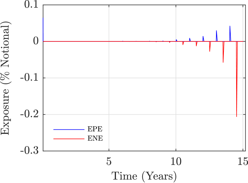
Black implied volatility, Vega sensitivity and Vega Risk for different Black shifts
λ6msubscript𝜆6m\lambda_{6\text{m}} σ6mBlksuperscriptsubscript𝜎6mBlk\sigma_{6\text{m}}^{\text{Blk}} ν𝜈\nu VR
0.010.010.01 0.22840.22840.2284 21 522 0242152202421\,522\,024 4 914 73549147354\,914\,735
0.040.040.04 0.13020.13020.1302 38 342 9833834298338\,342\,983 4 992 72449927244\,992\,724
0.060.060.06 0.07930.07930.0793 63 259 7026325970263\,259\,702 5 016 37850163785\,016\,378
0.080.080.08 0.06290.06290.0629 79 814 0667981406679\,814\,066 5 021 57850215785\,021\,578
0.100.100.10 0.05210.05210.0521 96 350 0569635005696\,350\,056 5 024 34550243455\,024\,345
Table 6: 5x10 years ATM physically settled European payer Swaption EUR 100 Mio notional, comparison between Black implied volatility σ6mBlk(t0)superscriptsubscript𝜎6mBlksubscript𝑡0\sigma_{6\text{m}}^{\text{Blk}}(t_{0}), Vega sensitivity ν(t0)𝜈subscript𝑡0\nu(t_{0}) and Vega Risk VR(t0)subscript𝑡0(t_{0}) at time step t0subscript𝑡0t_{0} for different Black shift values λ6msubscript𝜆6m\lambda_{6\text{m}}. Calculation approach as in eq. 5.8, with ϵσ=0.01subscriptitalic-ϵ𝜎0.01\epsilon_{\sigma}=0.01 and ϵη=0.04subscriptitalic-ϵ𝜂0.04\epsilon_{\eta}=0.04.

As can be seen, although a large impact on Black implied volatility and Vega sensitivity, the impact on Vega Risk is negligible as it is given by the product of the two quantities (see eq. C.8). More in detail, compared to the value observed at time step t0subscript𝑡0t_{0}, i.e. λ6m=0.01subscript𝜆6m0.01\lambda_{6\text{m}}=0.01, the various Black shifts considered produce Vega Risk values differing up to a maximum of 2%. This leads us to conclude that λxsubscript𝜆𝑥\lambda_{x} values larger than those observed at t0subscript𝑡0t_{0} ensure the inversion of the Black formula for each path with an acceptable loss of accuracy in Vega Risk. For this reason we set λ6m=0.06subscript𝜆6m0.06\lambda_{6\text{m}}=0.06.
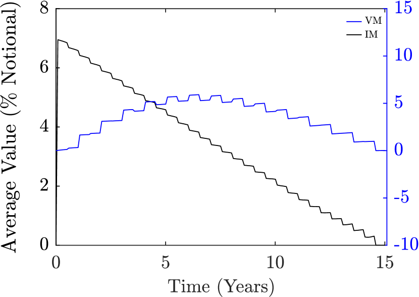
5.4 XVA Sensitivities to CSA Parameters

The aim of this section is to analyse the impacts of CSA parameters on XVA figures by assessing if collateralized CVA/DVA converges to uncollateralized ones for increasing values of threshold K and minimum transfer amount MTA, keeping other model parameters as in tab. 2. The results with respect to the length of MPoR l𝑙l are not reported since no significant impacts were found.
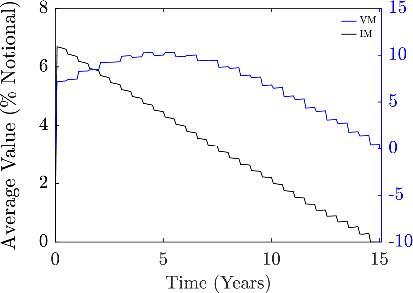
In carrying out the analysis we distinguished between the following three collateralization schemes:

  1. 1.

    CVA/DVA with VM only;

  2. 2.

    CVA/DVA with VM and IM, with K and MTA applied on VM only;

  3. 3.

    CVA/DVA with VM and IM, with K and MTA applied on both VM and IM.

Convergence diagrams for the 15 years ATM payer Swap are shown in figs. 13

(a) CVA with VM for different K, no MTA.
Refer to caption
(b) CVA with VM for different MTA, no K.
Refer to caption
(c) CVA with VM and IM for different K on VM only, no MTA.
Refer to caption
(d) CVA with VM and IM for different MTA on VM only, no K.
Refer to caption
(e) CVA with VM and IM for different K on VM and IM, no MTA.
Refer to caption
(f) CVA with VM and IM for different MTA on VM and IM, no K.
Refer to caption
Figure 13: 15 years ATM payer Swap EUR 100 Mio notional, collateralized CVA convergence to uncollateralized case with respect to threshold (K, left-hand side) and minimum transfer amount (MTA, right-hand side), keeping other model parameters as in tab. 2. Top panels: CVA with VM, mid panels: CVA with VM and IM with K/MTA only on VM, bottom panels: CVA and with VM and IM with K/MTA on both margins. Grey areas: collateralized CVA 3σ3𝜎3\sigma confidence intervals, dashed lines: 3σ3𝜎3\sigma uncollateralized CVA confidence intervals. Convergence to uncollateralized CVA is reached for top and bottom panels for smaller values of K compared to MTA, to confirm that K introduces higher friction.

and 14.

(a) DVA with VM for different K, no MTA.
Refer to caption
(b) DVA with VM for different MTA, no K.
Refer to caption
(c) DVA with VM and IM for different K on VM only, no MTA.
Refer to caption
(d) DVA with VM and IM for different MTA on VM only, no K.
Refer to caption
(e) DVA with VM and IM for different K on VM and IM, no MTA.
Refer to caption
(f) DVA with VM and IM for different MTA on VM and IM, no K.
Refer to caption
Figure 14: 15 years ATM payer Swap EUR 100 Mio notional, collateralized DVA convergence to uncollateralized case with respect to threshold (K, left-hand side) and minimum transfer amount (MTA, right-hand side), keeping other model parameters as in tab. 2. Top panels: DVA with VM, mid panels: DVA with VM and IM with K/MTA only on VM, bottom panels: DVA and with VM and IM with K/MTA on both margins. Grey areas: collateralized DVA 3σ3𝜎3\sigma confidence intervals, dashed lines: 3σ3𝜎3\sigma uncollateralized DVA confidence intervals. Analogous considerations of fig.13.

In particular, left-hand side panels show CVA/DVA convergence with respect to K, with MTA=0MTA0\text{MTA}=0 EUR and l=2𝑙2l=2 days; conversely, right-hand side panels show the convergence with respect to MTA, with K=0K0\text{K}=0 EUR and l=2𝑙2l=2 days. As can be seen, case 1. (top panels) and case 3. (bottom panels) display similar results except for small values of K and MTA, thus IM is ineffective when significant frictions are considered. Instead, case 2. (middle panels) displays collateralized CVA/DVA not converging to uncollateralized ones, this means that without frictions IM is effective in reducing residual credit exposure. Furthermore, the results suggest that K leads to a faster convergence to uncollateralized figures compared to MTA; e.g. in case 1. K=5K5\text{K}=5 Mio EUR leads to an increase in absolute terms of approx. 5700% in CVA and 3600% in DVA with respect to the reference case (see tab. 2), while MTA=5MTA5\text{MTA}=5 Mio EUR leads to an increase of approx. 1300% in CVA and 1100% in DVA. As expected, K introduces an higher degree of friction since determining the maximum amount of allowed unsecured exposure; on the other hand, MTA governs only the minimum amount for each margin call, therefore significant impacts can be observed only for large values (see eqs. 3.2 and 3.8). The 5x10 years ATM physically settled European payer Swaption displays same results and is not reported.
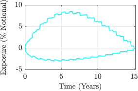
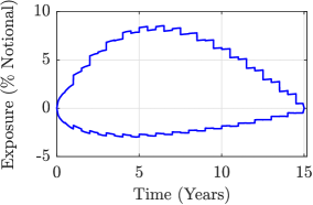
A focus on the effects of K on collateralized exposure is shown in fig. 15, which displays EPE/ENE for the 15 years Swap (left-hand side panels) and the 5x10 years ATM physically settled European payer Swaption (right-hand side panels) for the three collateralization schemes above, for different values of K (with MTA=0MTA0\text{MTA}=0 EUR and l=2𝑙2l=2 days).

(a) EPE and ENE Swap with VM, no MTA.
Refer to caption
(b) EPE and ENE Swaption with VM, no MTA.
Refer to caption
(c) EPE and ENE Swap with VM and IM, K on VM only, no MTA.
Refer to caption
(d) EPE and ENE Swaption with VM and IM, K on VM only, no MTA.
Refer to caption
(e) EPE and ENE Swap with VM and IM, K on VM and IM, no MTA.
Refer to caption
(f) EPE and ENE Swaption with VM and IM, K on VM and IM, no MTA.
Refer to caption
Figure 15: 15 years ATM payer Swap (left-hand side) and 5x10 years ATM physically settled European payer Swaption (right-hand side) EUR 100 Mio notional, collateralized EPE/ENE profiles for different values of threshold: K=0 Mio (blue lines), K = 1 Mio (cyan lines) and K = 5 Mio (red lines). Top panels: exposure with VM, mid panels: exposure with VM and IM with K only on VM, bottom panels: exposure with VM and IM with K on both margins. The residual exposure increases with K and IM becomes ineffective for large K. To enhance Swaption’s plots readability, we excluded collateralized EPE for time step t0subscript𝑡0t_{0} as not mitigated by collateral, in particular EPE(t0subscript𝑡0t_{0}) corresponds to Swaption’s price: 5 030 423 EUR (approx. 5%percent55\% of the notional). Other model parameters as in tab. 2. Quantities expressed as a percentage of the notional.

Focusing on the Swap with VM (top panel), the average EPE (ENE) over the time steps, expressed as a percentage of the notional, is equal to 0.08%percent0.080.08\%, 0.62%percent0.620.62\% and 2.56%percent2.562.56\% (0.04%percent0.04-0.04\%, 0.31%percent0.31-0.31\% and 1.12%percent1.12-1.12\%), respectively for threshold values of 0, 1 and 5 EUR Mio. By adding IM with no threshold (middle panel), large part of residual exposure is suppressed: average EPE (ENE) is equal to 0.00%percent0.000.00\%, 0.04%percent0.040.04\% and 0.91%percent0.910.91\% (0.00%percent0.000.00\%, 0.02%percent0.02-0.02\% and 0.25%percent0.25-0.25\%) of the notional. By considering threshold also on IM (bottom panel), average EPE (ENE) is equal to 0.00%percent0.000.00\%, 0.14%percent0.140.14\% and 2.46%percent2.462.46\% (0.00%percent0.000.00\%, 0.06%percent0.06-0.06\% and 0.97%percent0.97-0.97\%) of the notional meaning that, as K increases, IM looses its effectiveness and EPE/ENE approach to those with only VM.

5.5 Monte Carlo Versus Analytical XVA

In sec. 2.4.3 we have shown that analytical solutions for eqs. 2.29 and 2.30 are available for uncollateralized Swaps. In particular, CVA and DVA of a payer (receiver) Swap can be represented as an integral over the values of a strip of co-terminal European payer (receiver) Swaptions and European receiver (payer) Swaptions respectively (see eqs. 2.35 and 2.36).

Comparison between CVA/DVA obtained with analytical approach and Monte Carlo approach
Item ΔtΔ𝑡\Delta t Analytical G2++ Analytical Black MC
CVA ATM Swap 12M 1 091 604-1091604-1\,091\,604* 1 016 082-1016082-1\,016\,082 1 119 629-1119629-1\,119\,629 (±plus-or-minus\pm 444%)
6M 1 157 012-1157012-1\,157\,012* 1 077 346-1077346-1\,077\,346 1 170 271-1170271-1\,170\,271 (±plus-or-minus\pm 444%)
3M 1 147 871-1147871-1\,147\,871* 1 067 726-1067726-1\,067\,726 1 172 139-1172139-1\,172\,139 (±plus-or-minus\pm 444%)
1M 1 152 567-1152567-1\,152\,567* 1 072 231-1072231-1\,072\,231 1 172 938-1172938-1\,172\,938 (±plus-or-minus\pm 444%)
1D 1 156 083-1156083-1\,156\,083* 1 075 398-1075398-1\,075\,398 1 173 296-1173296-1\,173\,296 (±plus-or-minus\pm 444%)
DVA ATM Swap 12M 454 023454023454\,023* 432 373432373432\,373 485 660485660485\,660 (±plus-or-minus\pm 888%)
6M 471 340471340471\,340* 449 890449890449\,890* 478 016478016478\,016 (±plus-or-minus\pm 999%)
3M 468 884468884468\,884* 447 358447358447\,358* 476 789476789476\,789 (±plus-or-minus\pm 999%)
1M 468 721468721468\,721* 447 369447369447\,369* 475 324475324475\,324 (±plus-or-minus\pm 999%)
1D 469 562469562469\,562* 448 170448170448\,170* 474 469474469474\,469 (±plus-or-minus\pm 999%)
CVA OTM Swap 12M 744 144-744144-744\,144* 698 128-698128-698\,128* 732 977-732977-732\,977 (±plus-or-minus\pm 666%)
6M 783 485-783485-783\,485* 735 481-735481-735\,481 778 892-778892-778\,892 (±plus-or-minus\pm 666%)
3M 773 913-773913-773\,913* 725 498-725498-725\,498 779 280-779280-779\,280 (±plus-or-minus\pm 666%)
1M 774 432-774432-774\,432* 726 025-726025-726\,025 779 085-779085-779\,085 (±plus-or-minus\pm 666%)
1D 775 955-775955-775\,955* 727 392-727392-727\,392 778 991-778991-778\,991 (±plus-or-minus\pm 666%)
DVA OTM Swap 12M 788 254788254788\,254 793 430793430793\,430 892 169892169892\,169 (±plus-or-minus\pm 666%)
6M 833 226833226833\,226* 840 902840902840\,902* 880 117880117880\,117 (±plus-or-minus\pm 666%)
3M 839 022839022839\,022* 847 065847065847\,065* 882 972882972882\,972 (±plus-or-minus\pm 666%)
1M 846 586846586846\,586* 855 381855381855\,381* 884 382884382884\,382 (±plus-or-minus\pm 666%)
1D 851 479851479851\,479* 860 467860467860\,467* 885 227885227885\,227 (±plus-or-minus\pm 666%)
Table 7: 15 years ATM payer Swap and 15 years OTM payer Swap EUR 100 Mio notional, comparison between CVA/DVA obtained with analytical approach and Monte Carlo approach. The strip of co-terminal Swaptions has been computed through G2++ pricing formula in the third column and through Black formula in the fourth column. Results included in MC error marked with an asterisk. In absolute terms, analytical formulas underestimate CVA and DVA values. The results obtained with G2++ always included in MC error (only one exception: DVA OTM Swap 12M granularity). Considerable differences are observed with analytical Black.

The numerical solution of eqs. 2.35 and 2.36 involves the discretization of the integrals on a grid of time points (see eqs. 2.37 and 2.38), with impacts in terms of precision of the results related to its granularity. Therefore, as for Monte Carlo model, we tested analytical formulas for different time steps frequencies. Moreover, given the model independent nature of this approach, we calculated Swaptions prices through both G2++ and Black formulas. The purpose is twofold: one one hand we want to test the results of the Monte Carlo approach, on the other hand we want to quantify the model risk stemming from the use of two alternative pricing formulas. More in detail, we calculated G2++ Swaptions prices by applying eq. B.12 and G2++ parameters in tab. 2. Regarding Black pricing formula, the most complex step regards the determination of implied volatility for the strip of co-terminal Swaptions. Starting from market Swaptions prices cube, we calibrated SABR parameters (see [43]) on each smile section (i.e. tenor-expiry combination) obtaining a SABR parameters cube; hence, we determined the implied volatility for each co-terminal Swaption using the SABR approximated closed formula linearly interpolating/extrapolating on calibrated parameters cube in correspondence of the tenor-expiry combination of each co-terminal Swaption.

The analysis has been carried out considering the 15 years ATM payer Swap and the 15 years OTM payer Swap. The results shown in tab. 7 suggest that, with respect to Monte Carlo approach (last column), analytical formulas underestimate CVA and DVA values in absolute terms. Moreover, the results obtained with analytical G2++ (third column) are always included in Monte Carlo error (marked with an asterisk), with the only exception represented by the DVA of the OTM Swap with annual time grid granularity, to confirm the robustness of the results of the Monte Carlo model. As regards the results obtained with a different dynamic (fourth column), considerable differences are observed, particularly in CVA which is included in Monte Carlo error only in one case, to demonstrate that a not negligible model risk exists. In terms of computational performance, the advantage of the analytical approach is several orders of magnitude greater than that of Monte Carlo approach: with a daily grid robust results can be obtained in only 1 minute, meaning that, for an uncollateralized Swap, the analytical approach can replace the Monte Carlo approach whereas performance is critical.

5.6 XVA Model Risk

According to the Regulation (EU) No 575/2013 (see [34]), financial institutions are required to apply prudent valuation to fair-valued positions (Art. 105). For prudent valuation is meant the calculation of specific Additional Valuation Adjustments (AVA), to be deducted from the Common Equity Tier 1 (CET1) capital (Art. 34), necessary to adjust the fair-value of a financial instrument in order to achieve a prudent value with an appropriate degree of certainty. The prudent value has to be computed considering the valuation risk factors listed in Art. 105 (par. 10-11) in order to mitigate the risk of losses deriving from the valuation uncertainty of the exit price of a financial instrument. These valuation risk factors are linked to the corresponding AVA described in the Commission Delegated Regulation (EU) 2016/101 (see [35]), where the degree of certainty is set at 90%.
In particular, the Model Risk (MoRi) AVA is envisaged in Art. 11 of [35] and comprises the valuation uncertainty linked to the potential existence of a range of different models or model calibrations used by market participants. This may occur e.g. when a unique model recognized as a clear market standard for computing the price of a certain financial instrument does not exist, or when a model allows for different parameterizations or numerical solution algorithms. Accordingly, for MoRi AVA the prudent value at a 90% confidence level corresponds to the 10th percentile of the distribution of the plausible prices obtained from different models/parameterizations202020Notice that we conventionally adopt positive/negative prices for assets/liabilities..

In this section we apply this framework to XVA by calculating a MoRi AVA based on the different models and parameterizations discussed in the sections above. In particular, we computed MoRi AVA AVAMoRi(t0)superscriptAVAMoRisubscript𝑡0\text{AVA}^{\text{MoRi}}(t_{0}) at time t0subscript𝑡0t_{0} starting from the following definition and avoiding the aggregation coefficient

AVAMoRi(t0)=V(t0;M)PV(t0;M),superscriptAVAMoRisubscript𝑡0𝑉subscript𝑡0𝑀PVsubscript𝑡0superscript𝑀\text{AVA}^{\text{MoRi}}(t_{0})=V(t_{0};M)-\text{PV}(t_{0};M^{*}), (5.9)

where:

  • -

    V(t0;M)=V0(t0)+XVA(t0;M)𝑉subscript𝑡0𝑀subscript𝑉0subscript𝑡0XVAsubscript𝑡0𝑀V(t_{0};M)=V_{0}(t_{0})+\text{XVA}\left(t_{0};M\right) is the fair-value of the instrument, intended as the price obtained from the target XVA framework M𝑀M, i.e. the model and the corresponding parameters which optimizes the trade-off between accuracy and performance (as reported in tab. 2);

  • -

    PV(t0;M)=V0(t0)+XVA(t0;M)PVsubscript𝑡0superscript𝑀subscript𝑉0subscript𝑡0XVAsubscript𝑡0superscript𝑀\text{PV}(t_{0};M^{*})=V_{0}(t_{0})+\text{XVA}(t_{0};M^{*}) is the prudent value obtained from the alternative XVA framework M{M1,,MN}superscript𝑀subscript𝑀1subscript𝑀𝑁M^{*}\in\left\{M_{1},\dots,M_{N}\right\}, which produces the price corresponding to the 10th percentile of the prices distribution obtained from the set of N+1𝑁1N+1 XVA frameworks. In other words, Msuperscript𝑀M^{*} ensures that one can exit the position at a price equal to or larger than PV(t0;M)PVsubscript𝑡0superscript𝑀\text{PV}(t_{0};M^{*}) with a degree of certainty equal to or larger than 90%212121Notice that, according to our conventions, PV(t0)V(t0)PVsubscript𝑡0𝑉subscript𝑡0\text{PV}(t_{0})\leq V(t_{0})..

In light of this, and since we are not considering the valuation uncertainty related to the base value V0(t0)subscript𝑉0subscript𝑡0V_{0}(t_{0}), eq. 5.9 becomes

AVAMoRi(t0)=XVA(t0;M)XVA(t0;M).superscriptAVAMoRisubscript𝑡0XVAsubscript𝑡0𝑀XVAsubscript𝑡0superscript𝑀\text{AVA}^{\text{MoRi}}(t_{0})=\text{XVA}(t_{0};M)-\text{XVA}(t_{0};M^{*}).\\ (5.10)

We built the XVA distribution by leveraging on the outcomes of the analyses described in the sections above. In particular, we considered XVA obtained from both standard and joint grids with different granularities ΔtΔ𝑡\Delta t (see sec. 5.1), different numbers of simulated paths NMCsubscript𝑁𝑀𝐶N_{MC} (see sec. 5.2), and analytical approach for uncollateralized Swaps with different time steps frequencies and pricing formulas for the strip of co-terminal Swaptions (see sec. 5.5).
We report in tabs. 8 and 9 the XVA distributions for the uncollateralized 15 years ATM payer Swap and for the uncollateralized 5x10 years ATM physically settled European payer Swaption, respectively. Similar results were obtained for the other collateralization schemes.

15 years ATM payer Swap, no collateral
XVA framework
Mjsubscript𝑀𝑗M_{j} Model Parameters CVA DVA XVA
Time grid ΔtΔ𝑡\Delta t NMCsubscript𝑁𝑀𝐶N_{MC}
M1subscript𝑀1M_{1} MC Joint 1M 100010001000 1 153 010-1153010-1\,153\,010 445 537445537445\,537 707 473-707473-707\,473
M2subscript𝑀2M_{2} MC Joint 1M 200020002000 1 162 820-1162820-1\,162\,820 460 853460853460\,853 701 967-701967-701\,967
M3subscript𝑀3M_{3} MC Joint 1M 300030003000 1 166 416-1166416-1\,166\,416 465 953465953465\,953 700 463-700463-700\,463**
M4subscript𝑀4M_{4} MC Joint 1M 17 0001700017\,000 1 169 232-1169232-1\,169\,232 469 590469590469\,590 699 642-699642-699\,642
M5subscript𝑀5M_{5} MC Joint 1M 16 0001600016\,000 1 169 479-1169479-1\,169\,479 469 905469905469\,905 699 574-699574-699\,574
M6subscript𝑀6M_{6} MC Joint 1M 18 0001800018\,000 1 169 580-1169580-1\,169\,580 470 026470026470\,026 699 554-699554-699\,554
M7subscript𝑀7M_{7} MC Joint 1M 19 0001900019\,000 1 170 243-1170243-1\,170\,243 470 898470898470\,898 699 345-699345-699\,345
M8subscript𝑀8M_{8} MC Joint 1M 900090009000 1 170 432-1170432-1\,170\,432 471 101471101471\,101 699 331-699331-699\,331
M9subscript𝑀9M_{9} MC Joint 1M 10 0001000010\,000 1 169 500-1169500-1\,169\,500 470 184470184470\,184 699 316-699316-699\,316
M10subscript𝑀10M_{10} MC Joint 1M 11 0001100011\,000 1 169 599-1169599-1\,169\,599 470 326470326470\,326 699 273-699273-699\,273
M11subscript𝑀11M_{11} MC Joint 1M 20 0002000020\,000 1 170 511-1170511-1\,170\,511 471 327471327471\,327 699 184-699184-699\,184
M12subscript𝑀12M_{12} MC Joint 1M 12 0001200012\,000 1 170 445-1170445-1\,170\,445 471 424471424471\,424 699 021-699021-699\,021
M13subscript𝑀13M_{13} MC Joint 1M 15 0001500015\,000 1 171 196-1171196-1\,171\,196 472 365472365472\,365 698 831-698831-698\,831
M14subscript𝑀14M_{14} MC Joint 1D 500050005000 1 173 296-1173296-1\,173\,296 474 469474469474\,469 698 826-698826-698\,826
M15subscript𝑀15M_{15} MC Joint 1M 800080008000 1 171 461-1171461-1\,171\,461 472 833472833472\,833 698 628-698628-698\,628
M16subscript𝑀16M_{16} MC Joint 1M 13 0001300013\,000 1 171 579-1171579-1\,171\,579 473 037473037473\,037 698 542-698542-698\,542
M17subscript𝑀17M_{17} MC Joint 1M 14 0001400014\,000 1 171 638-1171638-1\,171\,638 473 143473143473\,143 698 495-698495-698\,495
M18subscript𝑀18M_{18} MC Joint 1M 400040004000 1 171 633-1171633-1\,171\,633 474 013474013474\,013 697 620-697620-697\,620
M𝑀M MC Joint 1M 500050005000 1 172 938-1172938-1\,172\,938 475 324475324475\,324 697 614-697614-697\,614*
M19subscript𝑀19M_{19} MC Joint 1M 700070007000 1 174 536-1174536-1\,174\,536 476 932476932476\,932 697 604-697604-697\,604
M20subscript𝑀20M_{20} MC Standard 1M 500050005000 1 172 940-1172940-1\,172\,940 475 340475340475\,340 697 601-697601-697\,601
M21subscript𝑀21M_{21} MC Joint 1M 600060006000 1 175 033-1175033-1\,175\,033 478 215478215478\,215 696 818-696818-696\,818
M22subscript𝑀22M_{22} MC Joint 3M 500050005000 1 172 139-1172139-1\,172\,139 476 789476789476\,789 695 350-695350-695\,350
M23subscript𝑀23M_{23} MC Standard 3M 500050005000 1 172 144-1172144-1\,172\,144 476 839476839476\,839 695 304-695304-695\,304
M24subscript𝑀24M_{24} MC Joint 6M 500050005000 1 170 271-1170271-1\,170\,271 478 016478016478\,016 692 255-692255-692\,255
M25subscript𝑀25M_{25} MC Standard 6M 500050005000 1 170 249-1170249-1\,170\,249 478 016478016478\,016 692 233-692233-692\,233
M26subscript𝑀26M_{26} Analytical G2++ Standard 1D NA 1 156 083-1156083-1\,156\,083 469 562469562469\,562 686 520-686520-686\,520
M27subscript𝑀27M_{27} Analytical G2++ Standard 6M NA 1 157 012-1157012-1\,157\,012 471 340471340471\,340 685 672-685672-685\,672
M28subscript𝑀28M_{28} Analytical G2++ Standard 1M NA 1 152 567-1152567-1\,152\,567 468 721468721468\,721 683 846-683846-683\,846
M29subscript𝑀29M_{29} Analytical G2++ Standard 3M NA 1 147 871-1147871-1\,147\,871 468 884468884468\,884 678 987-678987-678\,987
M30subscript𝑀30M_{30} Analytical G2++ Standard 12M NA 1 091 604-1091604-1\,091\,604 454 023454023454\,023 637 581-637581-637\,581
M31subscript𝑀31M_{31} MC Joint 12M 500050005000 1 119 629-1119629-1\,119\,629 485 660485660485\,660 633 968-633968-633\,968
M32subscript𝑀32M_{32} MC Standard 12M 500050005000 1 116 254-1116254-1\,116\,254 488 095488095488\,095 628 159-628159-628\,159
M33subscript𝑀33M_{33} Analytical Black Standard 6M NA 1 077 346-1077346-1\,077\,346 449 890449890449\,890 627 456-627456-627\,456
M34subscript𝑀34M_{34} Analytical Black Standard 1D NA 1 075 398-1075398-1\,075\,398 448 170448170448\,170 627 229-627229-627\,229
M35subscript𝑀35M_{35} Analytical Black Standard 1M NA 1 072 231-1072231-1\,072\,231 447 369447369447\,369 624 862-624862-624\,862
M36subscript𝑀36M_{36} Analytical Black Standard 3M NA 1 067 726-1067726-1\,067\,726 447 358447358447\,358 620 369-620369-620\,369
M37subscript𝑀37M_{37} Analytical Black Standard 12M NA 1 016 082-1016082-1\,016\,082 432 373432373432\,373 583 709-583709-583\,709
XVA(t0;M)subscript𝑡0𝑀(t_{0};M) 697 614-697614-697\,614
XVA(t0;M3)subscript𝑡0subscript𝑀3(t_{0};M_{3}) 700 463-700463-700\,463
AVA(t0)MoRi{}^{\text{MoRi}}(t_{0}) 284928492849
Table 8: 15 years ATM payer Swap EUR 100 Mio notional, no collateral. Distribution of plausible XVA; each row represents a different combination of model and parameters. XVA obtained from target framework M𝑀M optimizing the trade-off between accuracy and performance denoted by an asterisk while prudent XVA at a confidence level of 90% obtained from framework M3subscript𝑀3M_{3} denoted by double asterisk.
5x10 years ATM payer Swaption, no collateral
XVA framework
Mjsubscript𝑀𝑗M_{j} Model Parameters CVA DVA XVA
Time grid ΔtΔ𝑡\Delta t NMCsubscript𝑁𝑀𝐶N_{MC}
M1subscript𝑀1M_{1} MC Joint 1M 700070007000 824 079-824079-824\,079 36 1923619236\,192 787 887-787887-787\,887
M2subscript𝑀2M_{2} MC Joint 1M 600060006000 822 059-822059-822\,059 36 0343603436\,034 786 025-786025-786\,025**
M3subscript𝑀3M_{3} MC Joint 1D 500050005000 819 616-819616-819\,616 36 3673636736\,367 783 249-783249-783\,249
M4subscript𝑀4M_{4} MC Joint 1M 800080008000 819 809-819809-819\,809 36 7333673336\,733 783 075-783075-783\,075
M𝑀M MC Joint 1M 500050005000 818 308-818308-818\,308 36 4183641836\,418 781 890-781890-781\,890*
M5subscript𝑀5M_{5} MC Standard 1M 500050005000 818 293-818293-818\,293 36 4263642636\,426 781 867-781867-781\,867
M6subscript𝑀6M_{6} MC Joint 1M 14 0001400014\,000 819 182-819182-819\,182 37 7413774137\,741 781 441-781441-781\,441
M7subscript𝑀7M_{7} MC Joint 3M 500050005000 817 396-817396-817\,396 36 5443654436\,544 780 851-780851-780\,851
M8subscript𝑀8M_{8} MC Joint 1M 15 0001500015\,000 818 526-818526-818\,526 37 6773767737\,677 780 849-780849-780\,849
M9subscript𝑀9M_{9} MC Joint 1M 20 0002000020\,000 818 405-818405-818\,405 37 5773757737\,577 780 828-780828-780\,828
M10subscript𝑀10M_{10} MC Standard 3M 500050005000 817 335-817335-817\,335 36 5653656536\,565 780 770-780770-780\,770
M11subscript𝑀11M_{11} MC Joint 1M 19 0001900019\,000 818 061-818061-818\,061 37 3903739037\,390 780 671-780671-780\,671
M12subscript𝑀12M_{12} MC Joint 1M 13 0001300013\,000 818 459-818459-818\,459 37 9383793837\,938 780 521-780521-780\,521
M13subscript𝑀13M_{13} MC Joint 1M 18 0001800018\,000 817 336-817336-817\,336 37 2153721537\,215 780 121-780121-780\,121
M14subscript𝑀14M_{14} MC Joint 1M 900090009000 817 778-817778-817\,778 37 7903779037\,790 779 988-779988-779\,988
M15subscript𝑀15M_{15} MC Joint 1M 16 0001600016\,000 816 860-816860-816\,860 37 2943729437\,294 779 566-779566-779\,566
M16subscript𝑀16M_{16} MC Joint 1M 400040004000 816 207-816207-816\,207 36 8773687736\,877 779 330-779330-779\,330
M17subscript𝑀17M_{17} MC Joint 1M 11 0001100011\,000 816 663-816663-816\,663 37 3393733937\,339 779 324-779324-779\,324
M18subscript𝑀18M_{18} MC Joint 1M 17 0001700017\,000 816 521-816521-816\,521 37 2293722937\,229 779 292-779292-779\,292
M19subscript𝑀19M_{19} MC Joint 1M 12 0001200012\,000 817 132-817132-817\,132 37 8703787037\,870 779 261-779261-779\,261
M20subscript𝑀20M_{20} MC Joint 6M 500050005000 815 745-815745-815\,745 36 7053670536\,705 779 040-779040-779\,040
M21subscript𝑀21M_{21} MC Standard 6M 500050005000 815 610-815610-815\,610 36 7373673736\,737 778 873-778873-778\,873
M22subscript𝑀22M_{22} MC Joint 1M 10 0001000010\,000 816 317-816317-816\,317 37 5843758437\,584 778 733-778733-778\,733
M23subscript𝑀23M_{23} MC Joint 1M 300030003000 808 845-808845-808\,845 37 4813748137\,481 771 364-771364-771\,364
M24subscript𝑀24M_{24} MC Joint 1M 200020002000 802 335-802335-802\,335 37 8903789037\,890 764 445-764445-764\,445
M25subscript𝑀25M_{25} MC Joint 1M 100010001000 790 761-790761-790\,761 41 9994199941\,999 748 761-748761-748\,761
M26subscript𝑀26M_{26} MC Joint 12M 500050005000 775 964-775964-775\,964 41 3574135741\,357 734 606-734606-734\,606
M27subscript𝑀27M_{27} MC Standard 12M 500050005000 772 699-772699-772\,699 42 0474204742\,047 730 651-730651-730\,651
XVA(t0;M)subscript𝑡0𝑀(t_{0};M) 781 890-781890-781\,890
XVA(t0;M2)subscript𝑡0subscript𝑀2(t_{0};M_{2}) 786 025-786025-786\,025
AVA(t0)MoRi{}^{\text{MoRi}}(t_{0}) 413541354135
Table 9: 5x10 years ATM physically settled European payer Swaption EUR 100 Mio notional, no collateral. Distribution of plausible XVA; each row represents a different combination of model and parameters. XVA obtained from target framework M𝑀M optimizing the trade-off between accuracy and performance denoted by an asterisk while prudent XVA at a confidence level of 90% obtained from framework M2subscript𝑀2M_{2} denoted by double asterisk.

Focusing on the Swap in tab. 8, in addition to the target XVA framework M𝑀M we considered N=37𝑁37N=37 alternative frameworks. The one producing a prudent XVA at 90% confidence level is framework M3subscript𝑀3{M_{3}}, namely the Monte Carlo model with the following parameterization: joint grid, Δt=1Δ𝑡1\Delta t=1M and NMC=3000subscript𝑁𝑀𝐶3000N_{MC}=3000, at which corresponds XVA(t0;M3)=700 463XVAsubscript𝑡0subscript𝑀3700463\text{XVA}(t_{0};M_{3})=-700\,463 EUR (denoted by double asterisk in tab. 8). The related MoRi AVA obtained from eq. 5.10 is AVAMoRi(t0)=2849superscriptAVAMoRisubscript𝑡02849\text{AVA}^{\text{MoRi}}(t_{0})=2849 EUR, which corresponds to 0.41%percent0.410.41\% of XVA(t0;M)XVAsubscript𝑡0𝑀\text{XVA}(t_{0};M). With reference to the Swaption in tab. 9, the framework producing prudent XVA at 90% confidence level is framework M2subscript𝑀2{M_{2}}, namely the Monte Carlo model with the following parameterization: joint grid, Δt=1Δ𝑡1\Delta t=1M and NMC=6000subscript𝑁𝑀𝐶6000N_{MC}=6000, at which corresponds XVA(t0;M2)=XVAsubscript𝑡0subscript𝑀2absent\text{XVA}(t_{0};M_{2})= 786 025786025-786\,025 EUR (denoted by double asterisk in tab. 9). The related MoRi AVA is AVAMoRi(t0)=4135superscriptAVAMoRisubscript𝑡04135\text{AVA}^{\text{MoRi}}(t_{0})=4135 EUR, which corresponds to 0.53%percent0.530.53\% of XVA(t0;M)XVAsubscript𝑡0𝑀\text{XVA}(t_{0};M).

6 Conclusions

We have shown that CVA/DVA pricing is subject to a significant model risk, especially in the presence of Variation and Initial margins. In fact, collateral simulation implies a greater computational effort, particularly when a “bump-and-run” approach is used for computing ISDA-SIMM dynamic IM. For this reason, it becomes necessary to avoid unnecessary workloads that would make the calculation unfeasible. A decrease in computing time can be obtained through additional modelling choices which turn out to be additional sources of model risk. In this context we have found a parameterization that offers an acceptable compromise between accuracy and performance.
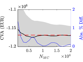
We have seen that a crucial element is the construction of a parsimonious time grid capable of capturing all periodical spikes arising in collateralized Swap’s exposure during the MPoR, having a material impact on CVA/DVA. To this end, we proposed a workaround which ensures to capture all spikes with an acceptable loss of precision in a reasonable time.

Regarding the number of simulated scenarios, we observed a convergence to “exact” value proxies even for a limited number of simulated paths, leaving room for an ulterior saving of computational time if necessary.

Further assumptions are required for the calculation of G2++ forward Vega sensitivities according to ISDA-SIMM prescriptions. In this case, the related model risk has been addressed by making sure that the proposed approximation produces results aligned with two alternative approaches both consistent with ISDA-SIMM definition at time t0subscript𝑡0t_{0} (i.e. valuation date) and by avoiding any arbitrary elements in the choice of the associated parameters.

Furthermore, we have shown that analytical formulas represent a useful tool for validating the results obtained through Monte Carlo approach provided that the same interest rates dynamic is considered, and can also be used for obtain reliable CVA/DVA for an uncollateralized Swap. Also in this case, model risk should be correctly addressed since different dynamics lead to different results.

Finally, the valuation uncertainty stemming from CVA/DVA pricing has been considered by calculating the related Model Risk Additional Valuation Adjustment (AVA) as envisaged in regulation [34, 35].

This work can be extended in different directions. The performance of the XVA framework can be enhanced by applying more advanced techniques, e.g. adjoint algorithmic differentiation (AAD) or Chebyshev decomposition to speed up and stabilize sensitivities calculation. The exposure engine can be extended to include other valuation adjustments, e.g. Funding Valuation Adjustment (FVA) and Margin Valuation Adjustment (MVA). More payoffs can be implemented and XVA can be computed at portfolio level.

Appendix A Market Data

The following tables report the market data considered in our work at 28 December 2018.

EURIBOR 6M curve Zero Coupon Bonds
t𝑡t (d) P(0;t)𝑃0𝑡P(0;t) t𝑡t (d) P(0;t)𝑃0𝑡P(0;t) t𝑡t (d) P(0;t)𝑃0𝑡P(0;t) t𝑡t (d) P(0;t)𝑃0𝑡P(0;t) t𝑡t (d) P(0;t)𝑃0𝑡P(0;t)
00 1.00001.00001.0000 311311311 1.00201.00201.0020 738738738 1.00361.00361.0036 548454845484 0.83550.83550.8355 10 5971059710\,597 0.66440.66440.6644
666 1.00001.00001.0000 339339339 1.00221.00221.0022 917917917 1.00331.00331.0033 584958495849 0.81950.81950.8195 10 9651096510\,965 0.65510.65510.6551
121212 1.00011.00011.0001 370370370 1.00241.00241.0024 110211021102 1.00221.00221.0022 621462146214 0.80390.80390.8039 11 3291132911\,329 0.64610.64610.6461
191919 1.00011.00011.0001 402402402 1.00251.00251.0025 146614661466 0.99770.99770.9977 658065806580 0.78900.78900.7890 11 6931169311\,693 0.63730.63730.6373
262626 1.00021.00021.0002 430430430 1.00271.00271.0027 183118311831 0.99020.99020.9902 694769476947 0.77470.77470.7747 12 0581205812\,058 0.62870.62870.6287
383838 1.00031.00031.0003 461461461 1.00281.00281.0028 219721972197 0.98000.98000.9800 731173117311 0.76120.76120.7612 12 4241242412\,424 0.62010.62010.6201
666666 1.00051.00051.0005 493493493 1.00301.00301.0030 256225622562 0.96750.96750.9675 767576757675 0.74840.74840.7484 12 7891278912\,789 0.61170.61170.6117
959595 1.00061.00061.0006 522522522 1.00311.00311.0031 292929292929 0.95310.95310.9531 804180418041 0.73610.73610.7361 13 1561315613\,156 0.60340.60340.6034
125125125 1.00081.00081.0008 552552552 1.00321.00321.0032 329332933293 0.93740.93740.9374 840684068406 0.72460.72460.7246 13 5201352013\,520 0.59530.59530.5953
157157157 1.00101.00101.0010 584584584 1.00331.00331.0033 365836583658 0.92080.92080.9208 877187718771 0.71360.71360.7136 13 8851388513\,885 0.58730.58730.5873
186186186 1.00121.00121.0012 614614614 1.00341.00341.0034 402340234023 0.90370.90370.9037 913891389138 0.70310.70310.7031 14 2501425014\,250 0.57960.57960.5796
217217217 1.00141.00141.0014 644644644 1.00351.00351.0035 438843884388 0.88630.88630.8863 950295029502 0.69320.69320.6932 14 6151461514\,615 0.57210.57210.5721
248248248 1.00161.00161.0016 675675675 1.00351.00351.0035 475347534753 0.86900.86900.8690 986798679867 0.68340.68340.6834 18 2681826818\,268 0.50460.50460.5046
278278278 1.00181.00181.0018 705705705 1.00361.00361.0036 512051205120 0.85200.85200.8520 10 2321023210\,232 0.67380.67380.6738 21 9202192021\,920 0.44610.44610.4461
Table 10: EURIBOR 6M Zero Coupon Curve.
OIS curve Zero Coupon Bonds
t𝑡t (d) P(0;t)𝑃0𝑡P(0;t) t𝑡t (d) P(0;t)𝑃0𝑡P(0;t) t𝑡t (d) P(0;t)𝑃0𝑡P(0;t) t𝑡t (d) P(0;t)𝑃0𝑡P(0;t) t𝑡t (d) P(0;t)𝑃0𝑡P(0;t)
00 1.00001.00001.0000 248248248 1.00251.00251.0025 675675675 1.00591.00591.0059 512051205120 0.86890.86890.8689 10 2321023210\,232 0.69420.69420.6942
333 1.00001.00001.0000 278278278 1.00281.00281.0028 705705705 1.00611.00611.0061 548454845484 0.85300.85300.8530 10 5971059710\,597 0.68500.68500.6850
555 1.00011.00011.0001 311311311 1.00311.00311.0031 738738738 1.00621.00621.0062 584958495849 0.83750.83750.8375 10 9651096510\,965 0.67580.67580.6758
666 1.00011.00011.0001 339339339 1.00331.00331.0033 110211021102 1.00631.00631.0063 621462146214 0.82240.82240.8224 12 7891278912\,789 0.63250.63250.6325
121212 1.00011.00011.0001 370370370 1.00361.00361.0036 146614661466 1.00331.00331.0033 658065806580 0.80790.80790.8079 14 6151461514\,615 0.59300.59300.5930
191919 1.00021.00021.0002 402402402 1.00391.00391.0039 183118311831 0.99750.99750.9975 694769476947 0.79390.79390.7939 18 2681826818\,268 0.52500.52500.5250
262626 1.00031.00031.0003 430430430 1.00421.00421.0042 219721972197 0.98880.98880.9888 731173117311 0.78070.78070.7807 21 9202192021\,920 0.46550.46550.4655
383838 1.00041.00041.0004 461461461 1.00441.00441.0044 256225622562 0.97780.97780.9778 767576757675 0.76820.76820.7682
666666 1.00071.00071.0007 493493493 1.00471.00471.0047 292929292929 0.96480.96480.9648 804180418041 0.75620.75620.7562
959595 1.00091.00091.0009 522522522 1.00491.00491.0049 329332933293 0.95010.95010.9501 840684068406 0.74480.74480.7448
125125125 1.00121.00121.0012 552552552 1.00521.00521.0052 365836583658 0.93460.93460.9346 877187718771 0.73400.73400.7340
157157157 1.00161.00161.0016 584584584 1.00541.00541.0054 402340234023 0.91830.91830.9183 913891389138 0.72350.72350.7235
186186186 1.00191.00191.0019 614614614 1.00561.00561.0056 438843884388 0.90180.90180.9018 950295029502 0.71350.71350.7135
217217217 1.00221.00221.0022 644644644 1.00581.00581.0058 475347534753 0.88530.88530.8853 986798679867 0.70370.70370.7037
Table 11: OIS Zero Coupon Curve (EONIA).
ATM Swaption prices matrix
ξ𝜉\xi/𝔗𝔗\mathfrak{T} 2 3 4 5 6 7 8 9 10 15 20 25 30
2 95 155 216 273 331 386 437 488 537 746 933 1108 1270
3 143 222 297 373 447 518 585 651 713 975 1221 1445 1653
4 185 279 371 460 548 632 715 793 865 1170 1459 1723 1976
5 221 328 432 534 634 731 824 913 996 1338 1666 1964 2250
6 248 367 481 594 705 810 912 1008 1101 1472 1832 2156 2471
7 271 399 523 644 763 876 986 1095 1200 1598 1980 2331 2674
8 290 427 560 690 818 940 1058 1171 1281 1705 2106 2487 2853
9 306 451 591 727 861 992 1116 1236 1355 1801 2227 2623 3007
10 320 473 620 765 904 1041 1170 1297 1427 1902 2344 2755 3164
12 342 503 663 816 967 1116 1257 1397 1528 2042 2516 2973 3390
15 368 544 713 879 1042 1198 1351 1505 1658 2225 2748 3230 3678
20 395 587 768 950 1131 1299 1469 1635 1794 2434 2961 3467 3927
25 417 620 812 1003 1188 1365 1537 1711 1878 2556 3086 3606 4082
30 432 640 842 1042 1229 1407 1571 1737 1906 2601 3136 3667 4164
Table 12: Quoted ATM Swaption Straddles (Physically settled LCH, N=10000𝑁10000N=10000 EUR), expiries and tenors in years on rows and columns respectively.
CDS spreads
t𝑡t (d) B C
180180180 91 24
360360360 105 29
720720720 125 48
108010801080 146 72
144014401440 163 99
180018001800 181 126
252025202520 200 159
360036003600 216 183
540054005400 219 195
720072007200 222 202
10 8001080010\,800 227 213
Table 13: CDS spread term structure for both counterparties (in bps).

Appendix B G2++ Swap and European Swaption Pricing

We present the generalization of G2++ pricing formulas for Swap and European Swaption in multi-curve framework and with time dependent (piece-wise constant) volatility parameters. In [38] it is shown that in single-curve framework European Swaption admits a closed formula. We derive European Swaption pricing formula in multi-curve framework by relying on the original derivation, expressing the multi-curve Swap price in a way which is formally equivalent to the single-curve one.

In single-curve framework, the price at time t𝑡t of an European Swaption expiring at Tesubscript𝑇𝑒T_{e} under the forward measure QTesuperscript𝑄subscript𝑇𝑒Q^{T_{e}} can be written as (we omit the filtration tsubscript𝑡\mathcal{F}_{t} in order to simplify the presentation)

Swaption(t;T,S,K,ω)=NP(t;Te)𝔼QTe{max[SwapSC(Te;T,S,K,ω,c);0]},=NP(t,Te)𝔼QTe{max[ω(P(Te;T0)i=1mciP(Te;Si));0]},\begin{split}\textbf{Swaption}(t;\textbf{T},\textbf{S},K,\omega)&=NP(t;T_{e})\mathbb{E}^{Q^{T_{e}}}\left\{\max\left[\textbf{Swap}^{\text{SC}}(T_{e};\textbf{T},\textbf{S},K,\omega,c);0\right]\right\},\\ &=NP(t,T_{e})\mathbb{E}^{Q^{T_{e}}}\left\{\max\left[\omega\left(P(T_{e};T_{0})-\sum_{i=1}^{m}c_{i}P(T_{e};S_{i})\right);0\right]\right\},\end{split} (B.1)

where ci=Kτ(Si1,Si)subscript𝑐𝑖𝐾𝜏subscript𝑆𝑖1subscript𝑆𝑖c_{i}=K\tau(S_{i-1},S_{i}) for i=1,,m1𝑖1𝑚1i=1,...,m-1 and cm=1+Kτ(Sm1,Sm)subscript𝑐𝑚1𝐾𝜏subscript𝑆𝑚1subscript𝑆𝑚c_{m}=1+K\tau(S_{m-1},S_{m}), with Sm=Tnsubscript𝑆𝑚subscript𝑇𝑛S_{m}=T_{n}. As already mentioned, [38] provides a closed formula for the expected value above under the G2++ model.

It can be shown that, in multi-curve framework, the price at time t𝑡t of a Swap’s floating coupon payment under the G2++ model is given by

Swapletfloat(t;Tj1,Tj)=N𝔼Q[D(t;Tj)Rx(Tj1,Tj)τR(Tj1,Tj)]=N[ϕd(Tj1;Tj)ϕx(Tj1;Tj)Pd(t;Tj1)Pd(t;Tj)],subscriptSwapletfloat𝑡subscript𝑇𝑗1subscript𝑇𝑗𝑁superscript𝔼𝑄delimited-[]𝐷𝑡subscript𝑇𝑗subscript𝑅𝑥subscript𝑇𝑗1subscript𝑇𝑗subscript𝜏𝑅subscript𝑇𝑗1subscript𝑇𝑗𝑁delimited-[]superscriptitalic-ϕ𝑑subscript𝑇𝑗1subscript𝑇𝑗superscriptitalic-ϕ𝑥subscript𝑇𝑗1subscript𝑇𝑗subscript𝑃𝑑𝑡subscript𝑇𝑗1subscript𝑃𝑑𝑡subscript𝑇𝑗\begin{split}\textbf{Swaplet}_{\text{float}}(t;T_{j-1},T_{j})&=N\mathbb{E}^{Q}\left[D(t;T_{j})R_{x}(T_{j-1},T_{j})\tau_{R}(T_{j-1},T_{j})\right]\\ &=N\left[\frac{\phi^{d}(T_{j-1};T_{j})}{\phi^{x}(T_{j-1};T_{j})}P_{d}(t;T_{j-1})-P_{d}(t;T_{j})\right],\\ \end{split} (B.2)

where ϕc(t;T)=exp{tTφc(u)𝑑u}superscriptitalic-ϕ𝑐𝑡𝑇superscriptsubscript𝑡𝑇superscript𝜑𝑐𝑢differential-d𝑢\phi^{c}(t;T)=\exp\left\{-\int_{t}^{T}\varphi^{c}(u)du\right\}, c{d,x}𝑐𝑑𝑥c\in\{d,x\} with d𝑑d and x𝑥x denoting respectively the discount 𝒞dsubscript𝒞𝑑\mathcal{C}_{d} and the forward 𝒞xsubscript𝒞𝑥\mathcal{C}_{x} curves.

Proof.
𝔼Q[D(t;Tj)Rx(Tj1,Tj)τR(Tj1,Tj)]=𝔼Q[D(t;Tj)1Px(Tj1;Tj)Px(Tj1;Tj)]=𝔼Q[ϕd(t;Tj)exp{tTjx(s)+y(s)ds}(1Px(Tj1;Tj)1)]=𝔼Q[ϕd(t;Tj)ϕx(Tj1;Tj)exp{tTj1x(s)+y(s)ds}𝔼Tj1Q[exp{Tj1Tjx(s)+y(s)ds}]𝔼Tj1Q[exp{Tj1Tjx(s)+y(s)ds}]]Pd(t;Tj)=𝔼Q[ϕd(t;Tj)ϕx(Tj1;Tj)exp{tTj1x(s)+y(s)ds}]Pd(t,Tj)=𝔼Q[ϕd(t;Tj1)ϕd(Tj1;Tj)ϕx(Tj1;Tj)exp{tTj1x(s)+y(s)ds}]Pd(t;Tj)=ϕd(Tj1;Tj)ϕx(Ti1;Tj)Pd(t;Tj1)Pd(t;Tj,)j.\begin{split}&\mathbb{E}^{Q}\left[D(t;T_{j})R_{x}(T_{j-1},T_{j})\tau_{R}(T_{j-1},T_{j})\right]\\ =&\mathbb{E}^{Q}\left[D(t;T_{j})\dfrac{1-P_{x}(T_{j-1};T_{j})}{P_{x}(T_{j-1};T_{j})}\right]\\ =&\mathbb{E}^{Q}\left[\phi^{d}(t;T_{j})\exp\left\{-\int_{t}^{T_{j}}x(s)+y(s)ds\right\}\left(\dfrac{1}{P_{x}(T_{j-1};T_{j})}-1\right)\right]\\ =&\mathbb{E}^{Q}\left[\dfrac{\phi^{d}(t;T_{j})}{\phi^{x}(T_{j-1};T_{j})}\exp\left\{-\int_{t}^{T_{j-1}}x(s)+y(s)ds\right\}\right.\\ &\qquad\qquad\qquad\qquad\left.\cdot\dfrac{\mathbb{E}_{T_{j-1}}^{Q}\left[\exp\left\{-\int_{T_{j-1}}^{T_{j}}x(s)+y(s)ds\right\}\right]}{\mathbb{E}_{T_{j-1}}^{Q}\left[\exp\left\{-\int_{T_{j-1}}^{T_{j}}x(s)+y(s)ds\right\}\right]}\right]-P_{d}(t;T_{j})\\ =&\mathbb{E}^{Q}\left[\dfrac{\phi^{d}(t;T_{j})}{\phi^{x}(T_{j-1};T_{j})}\exp\left\{-\int_{t}^{T_{j-1}}x(s)+y(s)ds\right\}\right]-P_{d}(t,T_{j})\\ =&\mathbb{E}^{Q}\left[\dfrac{\phi^{d}(t;T_{j-1})\phi^{d}(T_{j-1};T_{j})}{\phi^{x}(T_{j-1};T_{j})}\exp\left\{-\int_{t}^{T_{j-1}}x(s)+y(s)ds\right\}\right]-P_{d}(t;T_{j})\\ =&\frac{\phi^{d}(T_{j-1};T_{j})}{\phi^{x}(T_{i-1};T_{j})}P_{d}(t;T_{j-1})-P_{d}(t;T_{j},)\qquad\forall j.\end{split} (B.3)

Therefore the price of the Swap can be written as

SwapMC(t;T,S,K,ω)superscriptSwapMC𝑡TS𝐾𝜔\displaystyle\textbf{Swap}^{\text{MC}}(t;\textbf{T},\textbf{S},K,\omega)
=Nω[j=1n[ψ(Tj1;Tj)Pd(t;Tj1)Pd(t;Tj)]i=1mKτK(Si1,Si)Pd(t;Si)],absent𝑁𝜔delimited-[]superscriptsubscript𝑗1𝑛delimited-[]𝜓subscript𝑇𝑗1subscript𝑇𝑗subscript𝑃𝑑𝑡subscript𝑇𝑗1subscript𝑃𝑑𝑡subscript𝑇𝑗superscriptsubscript𝑖1𝑚𝐾subscript𝜏𝐾subscript𝑆𝑖1subscript𝑆𝑖subscript𝑃𝑑𝑡subscript𝑆𝑖\displaystyle=N\omega\Bigg{[}\sum_{j=1}^{n}\left[\psi(T_{j-1};T_{j})P_{d}(t;T_{j-1})-P_{d}(t;T_{j})\right]-\sum_{i=1}^{m}K\tau_{K}(S_{i-1},S_{i})P_{d}(t;S_{i})\Bigg{]}, (B.4)

with

ψ(Tj1;Tj)=ϕd(Tj1;Tj)ϕx(Tj1;Tj)=PdM(0;Tj)PdM(0;Tj1)PxM(0;Tj1)PxM(0;Tj),𝜓subscript𝑇𝑗1subscript𝑇𝑗superscriptitalic-ϕ𝑑subscript𝑇𝑗1subscript𝑇𝑗superscriptitalic-ϕ𝑥subscript𝑇𝑗1subscript𝑇𝑗superscriptsubscript𝑃𝑑𝑀0subscript𝑇𝑗superscriptsubscript𝑃𝑑𝑀0subscript𝑇𝑗1superscriptsubscript𝑃𝑥𝑀0subscript𝑇𝑗1superscriptsubscript𝑃𝑥𝑀0subscript𝑇𝑗\psi(T_{j-1};T_{j})=\frac{\phi^{d}(T_{j-1};T_{j})}{\phi^{x}(T_{j-1};T_{j})}=\frac{P_{d}^{M}(0;T_{j})}{P_{d}^{M}(0;T_{j-1})}\frac{P_{x}^{M}(0;T_{j-1})}{P_{x}^{M}(0;T_{j})}, (B.5)

where PcM(0;T)superscriptsubscript𝑃𝑐𝑀0𝑇P_{c}^{M}(0;T) is the currently observed ZCB maturing at T𝑇T and the second equality follows from

exp{Tj1Tjφc(u)𝑑u}=PcM(0;Tj)PcM(0;Tj1)exp{12[V(0;Tj)V(0;Tj1)]},superscriptsubscriptsubscript𝑇𝑗1subscript𝑇𝑗superscript𝜑𝑐𝑢differential-d𝑢superscriptsubscript𝑃𝑐𝑀0subscript𝑇𝑗superscriptsubscript𝑃𝑐𝑀0subscript𝑇𝑗112delimited-[]𝑉0subscript𝑇𝑗𝑉0subscript𝑇𝑗1\exp\left\{-\int_{T_{j-1}}^{T_{j}}\varphi^{c}(u)du\right\}=\frac{P_{c}^{M}(0;T_{j})}{P_{c}^{M}(0;T_{j-1})}\exp\left\{-\frac{1}{2}\left[V(0;T_{j})-V(0;T_{j-1})\right]\right\}, (B.6)

where V(t;Tj)𝑉𝑡subscript𝑇𝑗V(t;T_{j}) is the variance of the random variable I(t;Tj)=tTj[x(s)+y(s)]𝑑s𝐼𝑡subscript𝑇𝑗superscriptsubscript𝑡subscript𝑇𝑗delimited-[]𝑥𝑠𝑦𝑠differential-d𝑠I(t;T_{j})=\int_{t}^{T_{j}}[x(s)+y(s)]ds, which is normally distributed with mean M(t;Tj)𝑀𝑡subscript𝑇𝑗M(t;T_{j}) (see [38] for the proof). By considering the piece-wise constant volatility parameters introduced in sec. 2.3.1 we obtain the following equation

V(t;Tj)𝑉𝑡subscript𝑇𝑗\displaystyle V(t;T_{j}) =σ2a2i=uvΓi2[Ti+1Ti2eaTja(eaTi+1eaTi)e2aTj2a(e2aTi+1e2aTi)]absentsuperscript𝜎2superscript𝑎2superscriptsubscript𝑖𝑢𝑣superscriptsubscriptΓ𝑖2delimited-[]subscript𝑇𝑖1subscript𝑇𝑖2superscript𝑒𝑎subscript𝑇𝑗𝑎superscript𝑒𝑎subscript𝑇𝑖1superscript𝑒𝑎subscript𝑇𝑖superscript𝑒2𝑎subscript𝑇𝑗2𝑎superscript𝑒2𝑎subscript𝑇𝑖1superscript𝑒2𝑎subscript𝑇𝑖\displaystyle=\frac{\sigma^{2}}{a^{2}}\sum_{i=u}^{v}\Gamma_{i}^{2}\left[T_{i+1}-T_{i}-\frac{2e^{-aT_{j}}}{a}\left(e^{aT_{i+1}}-e^{aT_{i}}\right)-\frac{e^{-2aT_{j}}}{2a}\left(e^{2aT_{i+1}}-e^{2aT_{i}}\right)\right]
+η2b2i=uvΓi2[Ti+1Ti2ebTjb(ebTi+1ebTi)e2bTj2b(e2bTi+1e2bTi)]superscript𝜂2superscript𝑏2superscriptsubscript𝑖𝑢𝑣superscriptsubscriptΓ𝑖2delimited-[]subscript𝑇𝑖1subscript𝑇𝑖2superscript𝑒𝑏subscript𝑇𝑗𝑏superscript𝑒𝑏subscript𝑇𝑖1superscript𝑒𝑏subscript𝑇𝑖superscript𝑒2𝑏subscript𝑇𝑗2𝑏superscript𝑒2𝑏subscript𝑇𝑖1superscript𝑒2𝑏subscript𝑇𝑖\displaystyle+\frac{\eta^{2}}{b^{2}}\sum_{i=u}^{v}\Gamma_{i}^{2}\left[T_{i+1}-T_{i}-\frac{2e^{-bT_{j}}}{b}\left(e^{bT_{i+1}}-e^{bT_{i}}\right)-\frac{e^{-2bT_{j}}}{2b}\left(e^{2bT_{i+1}}-e^{2bT_{i}}\right)\right]
+2ρησabi=uvΓi2[Ti+1TieaTja(eaTi+1eaTi)ebTjb(ebTi+1ebTi)]2𝜌𝜂𝜎𝑎𝑏superscriptsubscript𝑖𝑢𝑣superscriptsubscriptΓ𝑖2delimited-[]subscript𝑇𝑖1subscript𝑇𝑖superscript𝑒𝑎subscript𝑇𝑗𝑎superscript𝑒𝑎subscript𝑇𝑖1superscript𝑒𝑎subscript𝑇𝑖superscript𝑒𝑏subscript𝑇𝑗𝑏superscript𝑒𝑏subscript𝑇𝑖1superscript𝑒𝑏subscript𝑇𝑖\displaystyle+\frac{2\rho\eta\sigma}{ab}\sum_{i=u}^{v}\Gamma_{i}^{2}\left[T_{i+1}-T_{i}-\frac{e^{-aT_{j}}}{a}\left(e^{aT_{i+1}}-e^{aT_{i}}\right)-\frac{e^{-bT_{j}}}{b}\left(e^{bT_{i+1}}-e^{bT_{i}}\right)\right]
+2ρησabi=uvΓi2[e(a+b)Tja+b(e(a+b)Ti+1e(a+b)Ti)],2𝜌𝜂𝜎𝑎𝑏superscriptsubscript𝑖𝑢𝑣superscriptsubscriptΓ𝑖2delimited-[]superscript𝑒𝑎𝑏subscript𝑇𝑗𝑎𝑏superscript𝑒𝑎𝑏subscript𝑇𝑖1superscript𝑒𝑎𝑏subscript𝑇𝑖\displaystyle+\frac{2\rho\eta\sigma}{ab}\sum_{i=u}^{v}\Gamma_{i}^{2}\left[\frac{e^{-(a+b)T_{j}}}{a+b}\left(e^{(a+b)T_{i+1}}-e^{(a+b)T_{i}}\right)\right], (B.7)

where here we assumed that Tu=tsubscript𝑇𝑢𝑡T_{u}=t and Tv+1=Tjsubscript𝑇𝑣1subscript𝑇𝑗T_{v+1}=T_{j}.

Now we are able to write the multi-curve Swap price in terms of the single-curve one assuming the existence of a vector of coefficient c^^𝑐\widehat{c} such that

SwapMC(t;T,S,K,ω)superscriptSwapMC𝑡TS𝐾𝜔\displaystyle\textbf{Swap}^{\text{MC}}(t;\textbf{T},\textbf{S},K,\omega) =c0SwapSC(t;T,S,K,ω,c^)absentsubscript𝑐0superscriptSwapSC𝑡TS𝐾𝜔^𝑐\displaystyle=c_{0}\ \textbf{Swap}^{\text{SC}}(t;\textbf{T},\textbf{S},K,\omega,\widehat{c})
=c0ω(P(t;T0)i=1mci^P(t;Ti)).absentsubscript𝑐0𝜔𝑃𝑡subscript𝑇0superscriptsubscript𝑖1𝑚^subscript𝑐𝑖𝑃𝑡subscript𝑇𝑖\displaystyle=c_{0}\ \omega\left(P(t;T_{0})-\sum_{i=1}^{m}\widehat{c_{i}}P(t;T_{i})\right). (B.8)

These coefficients are defined as follows

c0=ψ(T0;T1),cj^=c01[1ψ(Tj;Tj+1)𝟙{TjTn}+KτK(Si,Si+1)𝟙{Tj=Si}],j=1,,n.\begin{split}c_{0}&=\psi(T_{0};T_{1}),\\ \widehat{c_{j}}&=c_{0}^{-1}\left[1-\psi(T_{j};T_{j+1})\mathds{1}_{\left\{T_{j}\neq T_{n}\right\}}+K\tau_{K}(S_{i},S_{i+1})\mathds{1}_{\left\{T_{j}=S_{i}\right\}}\right],\quad j=1,\dots,n.\\ \end{split} (B.9)

Consider for example a payer Swap with unitary notional and maturity 2 years with semi-annual floating leg and annual fixed leg, characterized by the schedules T={T0,T1,T2,T3,T4}Tsubscript𝑇0subscript𝑇1subscript𝑇2subscript𝑇3subscript𝑇4\textbf{T}=\{T_{0},T_{1},T_{2},T_{3},T_{4}\} and S={S0,S1,S2}Ssubscript𝑆0subscript𝑆1subscript𝑆2\textbf{S}=\{S_{0},S_{1},S_{2}\}, where T0=S0subscript𝑇0subscript𝑆0T_{0}=S_{0}, T2=S1subscript𝑇2subscript𝑆1T_{2}=S_{1} and T4=S2subscript𝑇4subscript𝑆2T_{4}=S_{2}. The price in multi-curve framework is given by

SwapMC(t;T,S,K,1)=Pd(t;T0)ψ(T0;T1)Pd(t;T1)[1ψ(T1;T2)]Pd(t;T2)[1ψ(T2;T3)+KτK(S0,S1)]Pd(t;T3)[1ψ(T3;T4)]Pd(t;T4)[1+KτK(S1,S2)],superscriptSwapMC𝑡TS𝐾1subscript𝑃𝑑𝑡subscript𝑇0𝜓subscript𝑇0subscript𝑇1subscript𝑃𝑑𝑡subscript𝑇1delimited-[]1𝜓subscript𝑇1subscript𝑇2subscript𝑃𝑑𝑡subscript𝑇2delimited-[]1𝜓subscript𝑇2subscript𝑇3𝐾subscript𝜏𝐾subscript𝑆0subscript𝑆1subscript𝑃𝑑𝑡subscript𝑇3delimited-[]1𝜓subscript𝑇3subscript𝑇4subscript𝑃𝑑𝑡subscript𝑇4delimited-[]1𝐾subscript𝜏𝐾subscript𝑆1subscript𝑆2\begin{split}\textbf{Swap}^{\text{MC}}(t;\textbf{T},\textbf{S},K,1)&=P_{d}(t;T_{0})\psi(T_{0};T_{1})-P_{d}(t;T_{1})\left[1-\psi(T_{1};T_{2})\right]\\ &-P_{d}(t;T_{2})\left[1-\psi(T_{2};T_{3})+K\tau_{K}(S_{0},S_{1})\right]-P_{d}(t;T_{3})\left[1-\psi(T_{3};T_{4})\right]\\ &-P_{d}(t;T_{4})\left[1+K\tau_{K}(S_{1},S_{2})\right],\\ \end{split} (B.10)

from which it is possible to recognize the following coefficients

c0=ψ(T0;T1)c1^=c01[1ψ(T1;T2)]c2^=c01[1ψ(T2;T3)+KτK(S0,S1)]c3^=c01[1ψ(T3;T4)]c4^=c01[1+KτK(S1;S2)].subscript𝑐0𝜓subscript𝑇0subscript𝑇1^subscript𝑐1superscriptsubscript𝑐01delimited-[]1𝜓subscript𝑇1subscript𝑇2^subscript𝑐2superscriptsubscript𝑐01delimited-[]1𝜓subscript𝑇2subscript𝑇3𝐾subscript𝜏𝐾subscript𝑆0subscript𝑆1^subscript𝑐3superscriptsubscript𝑐01delimited-[]1𝜓subscript𝑇3subscript𝑇4^subscript𝑐4superscriptsubscript𝑐01delimited-[]1𝐾subscript𝜏𝐾subscript𝑆1subscript𝑆2\begin{split}c_{0}&=\psi(T_{0};T_{1})\\ \widehat{c_{1}}&=c_{0}^{-1}\left[1-\psi(T_{1};T_{2})\right]\\ \widehat{c_{2}}&=c_{0}^{-1}\left[1-\psi(T_{2};T_{3})+K\tau_{K}(S_{0},S_{1})\right]\\ \widehat{c_{3}}&=c_{0}^{-1}\left[1-\psi(T_{3};T_{4})\right]\\ \widehat{c_{4}}&=c_{0}^{-1}\left[1+K\tau_{K}(S_{1};S_{2})\right].\end{split} (B.11)

At this point we are able to write the G2++ pricing formula for an European Swaption in multi-curve framework and with piece-wise constant volatility parameters ensuring the preservation of the proof in [38]

Swaption(t;T,S,K,ω)=NωPd(t;Te)+e12(xμxσx)2σx2π[Φ(ωh1(x))j=1nλj(x)e𝒦j(x)Φ(ωh2(x))]𝑑x,Swaption𝑡TS𝐾𝜔𝑁𝜔subscript𝑃𝑑𝑡subscript𝑇𝑒superscriptsubscriptsuperscript𝑒12superscript𝑥subscript𝜇𝑥subscript𝜎𝑥2subscript𝜎𝑥2𝜋delimited-[]Φ𝜔subscript1𝑥superscriptsubscript𝑗1𝑛subscript𝜆𝑗𝑥superscript𝑒subscript𝒦𝑗𝑥Φ𝜔subscript2𝑥differential-d𝑥\begin{split}&\textbf{Swaption}(t;\textbf{T},\textbf{S},K,\omega)\\ &=N\omega P_{d}(t;T_{e})\int_{-\infty}^{+\infty}\frac{e^{-\frac{1}{2}(\frac{x-\mu_{x}}{\sigma_{x}})^{2}}}{\sigma_{x}\sqrt{2\pi}}\left[\Phi(-\omega h_{1}(x))-\sum_{j=1}^{n}\lambda_{j}(x)e^{\mathcal{K}_{j}(x)}\Phi(-\omega h_{2}(x))\right]dx,\end{split} (B.12)

where

h1(x)subscript1𝑥\displaystyle h_{1}(x) =y¯μyσy1ρxy2ρxy(xμx)σx1ρxy2,absent¯𝑦subscript𝜇𝑦subscript𝜎𝑦1superscriptsubscript𝜌𝑥𝑦2subscript𝜌𝑥𝑦𝑥subscript𝜇𝑥subscript𝜎𝑥1superscriptsubscript𝜌𝑥𝑦2\displaystyle=\frac{\bar{y}-\mu_{y}}{\sigma_{y}\sqrt{1-\rho_{xy}^{2}}}-\frac{\rho_{xy}(x-\mu_{x})}{\sigma_{x}\sqrt{1-\rho_{xy}^{2}}}, (B.13)
h2(x)subscript2𝑥\displaystyle h_{2}(x) =h1(x)+(b,Te,Tj)σy1ρxy2,absentsubscript1𝑥𝑏subscript𝑇𝑒subscript𝑇𝑗subscript𝜎𝑦1superscriptsubscript𝜌𝑥𝑦2\displaystyle=h_{1}(x)+\mathcal{B}(b,T_{e},T_{j})\sigma_{y}\sqrt{1-\rho_{xy}^{2}}, (B.14)
λj(x)subscript𝜆𝑗𝑥\displaystyle\lambda_{j}(x) =cj^𝒜d(Te;Tj)e(a,Te,Tj)x,absent^subscript𝑐𝑗subscript𝒜𝑑subscript𝑇𝑒subscript𝑇𝑗superscript𝑒𝑎subscript𝑇𝑒subscript𝑇𝑗𝑥\displaystyle=\widehat{c_{j}}\mathcal{A}_{d}(T_{e};T_{j})e^{-\mathcal{B}(a,T_{e},T_{j})x}, (B.15)
𝒦j(x)subscript𝒦𝑗𝑥\displaystyle\mathcal{K}_{j}(x) =(b,Te,Tj)[μy12(1ρxy2)σy2(b,Te,Tj)+ρxyσyxμxσx],absent𝑏subscript𝑇𝑒subscript𝑇𝑗delimited-[]subscript𝜇𝑦121superscriptsubscript𝜌𝑥𝑦2superscriptsubscript𝜎𝑦2𝑏subscript𝑇𝑒subscript𝑇𝑗subscript𝜌𝑥𝑦subscript𝜎𝑦𝑥subscript𝜇𝑥subscript𝜎𝑥\displaystyle=-\mathcal{B}(b,T_{e},T_{j})\left[\mu_{y}-\frac{1}{2}(1-\rho_{xy}^{2})\sigma_{y}^{2}\mathcal{B}(b,T_{e},T_{j})+\rho_{xy}\sigma_{y}\frac{x-\mu_{x}}{\sigma_{x}}\right], (B.16)
𝒜c(t;Tj)subscript𝒜𝑐𝑡subscript𝑇𝑗\displaystyle\mathcal{A}_{c}(t;T_{j}) =PcM(0;Tj)PcM(0;Tj)exp(12V(0;Tj)+12V(0;t)+12V(t;Tj)),absentsuperscriptsubscript𝑃𝑐𝑀0subscript𝑇𝑗superscriptsubscript𝑃𝑐𝑀0subscript𝑇𝑗12𝑉0subscript𝑇𝑗12𝑉0𝑡12𝑉𝑡subscript𝑇𝑗\displaystyle=\frac{P_{c}^{M}(0;T_{j})}{P_{c}^{M}(0;T_{j})}\exp\left(-\frac{1}{2}V(0;T_{j})+\frac{1}{2}V(0;t)+\frac{1}{2}V(t;T_{j})\right), (B.17)
(z,t;Tj)𝑧𝑡subscript𝑇𝑗\displaystyle\mathcal{B}(z,t;T_{j}) =1ez(Tjt)z,z{a,b}.formulae-sequenceabsent1superscript𝑒𝑧subscript𝑇𝑗𝑡𝑧𝑧𝑎𝑏\displaystyle=\frac{1-e^{-z(T_{j}-t)}}{z},\quad z\in\{a,b\}. (B.18)

y¯=y¯(x)¯𝑦¯𝑦𝑥\bar{y}=\bar{y}(x) is the solution of the following equation

j=1ncj^𝒜d(Te;Tj)e(a,Te,Tj)x(b,Te,Tj)y¯=1,superscriptsubscript𝑗1𝑛^subscript𝑐𝑗subscript𝒜𝑑subscript𝑇𝑒subscript𝑇𝑗superscript𝑒𝑎subscript𝑇𝑒subscript𝑇𝑗𝑥𝑏subscript𝑇𝑒subscript𝑇𝑗¯𝑦1\sum_{j=1}^{n}\widehat{c_{j}}\mathcal{A}_{d}(T_{e};T_{j})e^{-\mathcal{B}(a,T_{e},T_{j})x-\mathcal{B}(b,T_{e},T_{j})\bar{y}}=1, (B.19)

and by setting Tu=tsubscript𝑇𝑢𝑡T_{u}=t and Tv+1=Tesubscript𝑇𝑣1subscript𝑇𝑒T_{v+1}=T_{e}

μxsubscript𝜇𝑥\displaystyle\mu_{x} =MxT(t;Te),absentsubscriptsuperscript𝑀𝑇𝑥𝑡subscript𝑇𝑒\displaystyle=-M^{T}_{x}(t;T_{e}), (B.20)
μysubscript𝜇𝑦\displaystyle\mu_{y} =MyT(t;Te),absentsubscriptsuperscript𝑀𝑇𝑦𝑡subscript𝑇𝑒\displaystyle=-M^{T}_{y}(t;T_{e}), (B.21)
σxsubscript𝜎𝑥\displaystyle\sigma_{x} =σ22ai=uvΓi2e2aTee2a(Ti+1Ti),absentsuperscript𝜎22𝑎superscriptsubscript𝑖𝑢𝑣superscriptsubscriptΓ𝑖2superscript𝑒2𝑎subscript𝑇𝑒superscript𝑒2𝑎subscript𝑇𝑖1subscript𝑇𝑖\displaystyle=\sqrt{\frac{\sigma^{2}}{2a}\sum_{i=u}^{v}\Gamma_{i}^{2}e^{-2aT_{e}}e^{2a(T_{i+1}-T_{i})}}, (B.22)
σysubscript𝜎𝑦\displaystyle\sigma_{y} =η22bi=uvΓi2e2bTee2b(Ti+1Ti),absentsuperscript𝜂22𝑏superscriptsubscript𝑖𝑢𝑣superscriptsubscriptΓ𝑖2superscript𝑒2𝑏subscript𝑇𝑒superscript𝑒2𝑏subscript𝑇𝑖1subscript𝑇𝑖\displaystyle=\sqrt{\frac{\eta^{2}}{2b}\sum_{i=u}^{v}\Gamma_{i}^{2}e^{-2bT_{e}}e^{2b(T_{i+1}-T_{i})}}, (B.23)
ρxysubscript𝜌𝑥𝑦\displaystyle\rho_{xy} =ρση(a+b)σxσy[1e(a+b)Te]i=uvΓi2e(a+b)(Ti+1Ti),absent𝜌𝜎𝜂𝑎𝑏subscript𝜎𝑥subscript𝜎𝑦delimited-[]1superscript𝑒𝑎𝑏subscript𝑇𝑒superscriptsubscript𝑖𝑢𝑣superscriptsubscriptΓ𝑖2superscript𝑒𝑎𝑏subscript𝑇𝑖1subscript𝑇𝑖\displaystyle=\frac{\rho\sigma\eta}{(a+b)\sigma_{x}\sigma_{y}}\left[1-e^{-(a+b)T_{e}}\right]\sum_{i=u}^{v}\Gamma_{i}^{2}e^{(a+b)(T_{i+1}-T_{i})}, (B.24)

where MxT(t;Te)subscriptsuperscript𝑀𝑇𝑥𝑡subscript𝑇𝑒M^{T}_{x}(t;T_{e}) and MyT(t;Te)subscriptsuperscript𝑀𝑇𝑦𝑡subscript𝑇𝑒M^{T}_{y}(t;T_{e}) are drift components stemming from the dynamics of the processes x𝑥x and y𝑦y under the forward measure T𝑇T

MxT(t;Te)subscriptsuperscript𝑀𝑇𝑥𝑡subscript𝑇𝑒\displaystyle M^{T}_{x}(t;T_{e}) =σ2ai=uvΓi2[eaTea(eaTi+1eaTi)ea(Te+T)2a(e2aTi+1e2aTi)]absentsuperscript𝜎2𝑎superscriptsubscript𝑖𝑢𝑣superscriptsubscriptΓ𝑖2delimited-[]superscript𝑒𝑎subscript𝑇𝑒𝑎superscript𝑒𝑎subscript𝑇𝑖1superscript𝑒𝑎subscript𝑇𝑖superscript𝑒𝑎subscript𝑇𝑒𝑇2𝑎superscript𝑒2𝑎subscript𝑇𝑖1superscript𝑒2𝑎subscript𝑇𝑖\displaystyle=\frac{\sigma^{2}}{a}\sum_{i=u}^{v}\Gamma_{i}^{2}\left[\frac{e^{-aT_{e}}}{a}\left(e^{aT_{i+1}}-e^{aT_{i}}\right)-\frac{e^{-a(T_{e}+T)}}{2a}\left(e^{2aT_{i+1}}-e^{2aT_{i}}\right)\right]
ρσηb(a+b)i=uvΓi2[eaTea(eaTi+1eaTi)e(aTe+bT)a+b(e(a+b)Ti+1e(a+b)Ti)],𝜌𝜎𝜂𝑏𝑎𝑏superscriptsubscript𝑖𝑢𝑣superscriptsubscriptΓ𝑖2delimited-[]superscript𝑒𝑎subscript𝑇𝑒𝑎superscript𝑒𝑎subscript𝑇𝑖1superscript𝑒𝑎subscript𝑇𝑖superscript𝑒𝑎subscript𝑇𝑒𝑏𝑇𝑎𝑏superscript𝑒𝑎𝑏subscript𝑇𝑖1superscript𝑒𝑎𝑏subscript𝑇𝑖\displaystyle-\frac{\rho\sigma\eta}{b(a+b)}\sum_{i=u}^{v}\Gamma_{i}^{2}\left[\frac{e^{-aT_{e}}}{a}\left(e^{aT_{i+1}}-e^{aT_{i}}\right)-\frac{e^{-(aT_{e}+bT)}}{a+b}\left(e^{(a+b)T_{i+1}}-e^{(a+b)T_{i}}\right)\right], (B.25)
MyT(t;Te)subscriptsuperscript𝑀𝑇𝑦𝑡subscript𝑇𝑒\displaystyle M^{T}_{y}(t;T_{e}) =η2bi=uvΓi2[1bebTe(ebTi+1ebTi)eb(Te+T)2b(e2bTi+1e2bTi)]absentsuperscript𝜂2𝑏superscriptsubscript𝑖𝑢𝑣superscriptsubscriptΓ𝑖2delimited-[]1𝑏superscript𝑒𝑏subscript𝑇𝑒superscript𝑒𝑏subscript𝑇𝑖1superscript𝑒𝑏subscript𝑇𝑖superscript𝑒𝑏subscript𝑇𝑒𝑇2𝑏superscript𝑒2𝑏subscript𝑇𝑖1superscript𝑒2𝑏subscript𝑇𝑖\displaystyle=\frac{\eta^{2}}{b}\sum_{i=u}^{v}\Gamma_{i}^{2}\left[\frac{1}{b}e^{-bT_{e}}\left(e^{bT_{i+1}}-e^{bT_{i}}\right)-\frac{e^{-b(T_{e}+T)}}{2b}\left(e^{2bT_{i+1}}-e^{2bT_{i}}\right)\right]
ρσηa(a+b)i=uvΓi2[ebTeb(ebTi+1ebTi)e(aTe+bT)a+b(e(a+b)Ti+1e(a+b)Ti)].𝜌𝜎𝜂𝑎𝑎𝑏superscriptsubscript𝑖𝑢𝑣superscriptsubscriptΓ𝑖2delimited-[]superscript𝑒𝑏subscript𝑇𝑒𝑏superscript𝑒𝑏subscript𝑇𝑖1superscript𝑒𝑏subscript𝑇𝑖superscript𝑒𝑎subscript𝑇𝑒𝑏𝑇𝑎𝑏superscript𝑒𝑎𝑏subscript𝑇𝑖1superscript𝑒𝑎𝑏subscript𝑇𝑖\displaystyle-\frac{\rho\sigma\eta}{a(a+b)}\sum_{i=u}^{v}\Gamma_{i}^{2}\left[\frac{e^{-bT_{e}}}{b}\left(e^{bT_{i+1}}-e^{bT_{i}}\right)-\frac{e^{-(aT_{e}+bT)}}{a+b}\left(e^{(a+b)T_{i+1}}-e^{(a+b)T_{i}}\right)\right]. (B.26)

Appendix C ISDA-SIMM for Swaps and European Swaptions

We describe the application of the Standard Initial Margin Model to Swaps and European Swaptions at trade level. We considered ISDA-SIMM Version 2.1 in order to be consistent with the valuation date considered (28 December 2018) 222222Version 2.1 was effective from 1 December 2018 to 30 November 2019 when Version 2.2 was published. used in our analyses. Further details may be found in [41]. As shown in sec. 3.3.1, IM for a Swap and an European Swaption is given by

IMSwapsuperscriptIMSwap\displaystyle\text{IM}^{\text{Swap}} =DeltaMarginIR,absentsuperscriptDeltaMarginIR\displaystyle=\text{DeltaMargin}^{\text{IR}}, (C.1)
IMSwptsuperscriptIMSwpt\displaystyle\text{IM}^{\text{Swpt}} =DeltaMarginIR+VegaMarginIR+CurvatureMarginIR.absentsuperscriptDeltaMarginIRsuperscriptVegaMarginIRsuperscriptCurvatureMarginIR\displaystyle=\text{DeltaMargin}^{\text{IR}}+\text{VegaMargin}^{\text{IR}}+\text{CurvatureMargin}^{\text{IR}}. (C.2)

The details on the calculation process for the three IM components are given in paragraphs below.

C.1 Delta Margin for Interest Rate Risk Class

Delta Margin for IR Risk Class is computed through the following step-by-step process.

  1. 1.

    Calculation of IR Delta sensitivities vector

    Δc=[Δ2wc,Δ1mc,Δ3mc,Δ6mc,Δ1yc,Δ2yc,Δ3yc,Δ5yc,Δ10yc,Δ15yc,Δ20yc,Δ30yc],superscriptΔ𝑐subscriptsuperscriptΔ𝑐2wsubscriptsuperscriptΔ𝑐1msubscriptsuperscriptΔ𝑐3msubscriptsuperscriptΔ𝑐6msubscriptsuperscriptΔ𝑐1ysubscriptsuperscriptΔ𝑐2ysubscriptsuperscriptΔ𝑐3ysubscriptsuperscriptΔ𝑐5ysubscriptsuperscriptΔ𝑐10ysubscriptsuperscriptΔ𝑐15ysubscriptsuperscriptΔ𝑐20ysubscriptsuperscriptΔ𝑐30y\Delta^{c}=[\Delta^{c}_{2\text{w}},\Delta^{c}_{1\text{m}},\Delta^{c}_{3\text{m}},\Delta^{c}_{6\text{m}},\Delta^{c}_{1\text{y}},\Delta^{c}_{2\text{y}},\Delta^{c}_{3\text{y}},\Delta^{c}_{5\text{y}},\Delta^{c}_{10\text{y}},\Delta^{c}_{15\text{y}},\Delta^{c}_{20\text{y}},\Delta^{c}_{30\text{y}}], (C.3)

    where c{f,d}𝑐𝑓𝑑c\in\{f,d\}. See sec. 3.3.2 for details on definition and calculation methodology.

  2. 2.

    Calculation of Weighted Sensitivity WSj,c for the j𝑗j-th SIMM tenor through the following formula

    WSj,c=RWjΔjcCRb,subscriptWS𝑗𝑐subscriptRW𝑗subscriptsuperscriptΔ𝑐𝑗subscriptCR𝑏\text{WS}_{j,c}=\text{RW}_{j}\cdot\Delta^{c}_{j}\cdot\text{CR}_{b}, (C.4)

    where:

    • -

      RWj is the Risk Weight for the j𝑗j-th SIMM tenor (tab. 14). ISDA specifies three different vectors based upon the volatility of the currency in which the instrument is denominated232323Low Volatility currencies: JPY; Regular Volatility currencies: USD, EUR, GBP, CHF, AUD, NZD, CAD, SEK, NOK, DKK, HKD, KRW, SGD and TWD; High Volatility currencies: all other currencies.;

    • -

      ΔjcsubscriptsuperscriptΔ𝑐𝑗\Delta^{c}_{j} is Delta sensitivity corresponding to the j𝑗j-th SIMM tenor for the interest rate curve c𝑐c;

    • -

      CRb is the Concentration Risk Factor for the Currency Group b𝑏b. In this case ISDA specifies four Currency Groups based upon the volatility of the currency in which the instrument is denominated242424Low Volatility currencies: JPY; Regular Volatility well-traded currencies: USD, EUR, GBP; Regular Volatility less well-traded currencies: CHF, AUD, NZD, CAD, SEK, NOK, DKK, HKD, KRW, SGD, TWD; High Volatility currencies: all other currencies. . CRb is calculated as follows

      CRb=max{1,(|j,cΔjc|Tb)12},subscriptCR𝑏max1superscriptsubscript𝑗𝑐subscriptsuperscriptΔ𝑐𝑗subscriptT𝑏12\text{CR}_{b}=\text{max}\left\{1,\left(\frac{|\sum_{j,c}\Delta^{c}_{j}|}{\text{T}_{b}}\right)^{\frac{1}{2}}\right\}, (C.5)

      where Tb is the Concentration Threshold for the Currency Group b𝑏b. For Regular Volatility well-traded currencies T=b{}_{b}= 210 USD Mio/bp.

  3. 3.

    Calculation of Delta Margin through the aggregation of Weighted Sensitivities

    DeltaMarginIR=c,jWSj,c2+c,j(k,l)(c,j)ϕc,kρj,lWSj,cWSl,k,superscriptDeltaMarginIRsubscript𝑐𝑗superscriptsubscriptWS𝑗𝑐2subscript𝑐𝑗subscript𝑘𝑙𝑐𝑗subscriptitalic-ϕ𝑐𝑘subscript𝜌𝑗𝑙subscriptWS𝑗𝑐subscriptWS𝑙𝑘\text{DeltaMargin}^{\text{IR}}=\sqrt{\sum_{c,j}\text{WS}_{j,c}^{2}+\sum_{c,j}\sum_{(k,l)\neq(c,j)}\phi_{c,k}\rho_{j,l}\text{WS}_{j,c}\text{WS}_{l,k}}, (C.6)

    where:

    • -

      ϕc,k=subscriptitalic-ϕ𝑐𝑘absent\phi_{c,k}= 98% is the correlation between interest rate curves of the same currency;

    • -

      ρj,lsubscript𝜌𝑗𝑙\rho_{j,l} is the correlation matrix between SIMM tenors (tab. 15).

C.2 Vega Margin for Interest Rate Risk Class

Vega Margin for IR Risk Class is computed through the following step-by-step process.

  1. 1.

    Calculation of Vega Risks vector

    VR=[VR2w,VR1m,VR3m,VR6m,VR1y,VR2y,VR3y,VR5y,VR10y,VR15y,VR20y,VR30y],VRsubscriptVR2wsubscriptVR1msubscriptVR3msubscriptVR6msubscriptVR1ysubscriptVR2ysubscriptVR3ysubscriptVR5ysubscriptVR10ysubscriptVR15ysubscriptVR20ysubscriptVR30y\text{VR}=[\text{VR}_{2\text{w}},\text{VR}_{1\text{m}},\text{VR}_{3\text{m}},\text{VR}_{6\text{m}},\text{VR}_{1\text{y}},\text{VR}_{2\text{y}},\text{VR}_{3\text{y}},\text{VR}_{5\text{y}},\text{VR}_{10\text{y}},\text{VR}_{15\text{y}},\text{VR}_{20\text{y}},\text{VR}_{30\text{y}}], (C.7)

    where:

    VRj=νjσjBlk,subscriptVR𝑗subscript𝜈𝑗subscriptsuperscript𝜎Blk𝑗\text{VR}_{j}=\nu_{j}\cdot\sigma^{\text{Blk}}_{j}, (C.8)

    is the Vega Risk for an European Swaption with expiry equal to tenor j𝑗j, with νjsubscript𝜈𝑗\nu_{j} and σjBlksubscriptsuperscript𝜎Blk𝑗\sigma^{\text{Blk}}_{j} being, respectively, IR Vega sensitivity and Black implied volatility. See sec. 3.3.2 for details on definition and calculation methodology.

  2. 2.

    Calculation of Vega Risk Exposure VREj for the j𝑗j-th SIMM expiry through the following formula

    VREj=VRWIRVRjVCRb,subscriptVRE𝑗superscriptVRWIRsubscriptVR𝑗subscriptVCR𝑏\text{VRE}_{j}=\text{VRW}^{\text{IR}}\cdot\text{VR}_{j}\cdot\text{VCR}_{b}, (C.9)

    where:

    • -

      VRW=IR0.16{}^{\text{IR}}=0.16 is the Vega Risk Weight for IR Risk Class;

    • -

      VCRb is the Vega Concentration Risk Factor for the Currency Group b𝑏b calculated as252525See footnote 24.

      VCRb=max{1,(|jVRj|VTb)12},subscriptVCR𝑏max1superscriptsubscript𝑗subscriptVR𝑗subscriptVT𝑏12\text{VCR}_{b}=\text{max}\left\{1,\left(\frac{|\sum_{j}\text{VR}_{j}|}{\text{VT}_{b}}\right)^{\frac{1}{2}}\right\}, (C.10)

      where VTb is the Concentration Threshold for the Currency Group b𝑏b. For Regular Volatility well-traded currencies T=b2200{}_{b}=2200 USD Mio.

  3. 3.

    Calculation of Vega Margin through the aggregation of the Vega Risk Exposures

    VegaMarginIR=jVREj2+jljρj,lVREjVREl,superscriptVegaMarginIRsubscript𝑗superscriptsubscriptVRE𝑗2subscript𝑗subscript𝑙𝑗subscript𝜌𝑗𝑙subscriptVRE𝑗subscriptVRE𝑙\text{VegaMargin}^{\text{IR}}=\sqrt{\sum_{j}\text{VRE}_{j}^{2}+\sum_{j}\sum_{l\neq j}\rho_{j,l}\text{VRE}_{j}\text{VRE}_{l}}, (C.11)

    where ρj,lsubscript𝜌𝑗𝑙\rho_{j,l} is the correlation matrix between expiries (tab. 15).

C.3 Curvature Margin for Interest Rate Risk Class

Curvature Margin for IR Risk Class is computed through the following step-by-step process.

  1. 1.

    Calculation of Curvature Risk vector by applying a Scaling Function (tab. 16) to Vega Risk vector calculated for Vega Margin, in particular, for the j𝑗j-th element

    CVRj=SF(tj)VRj,subscriptCVR𝑗SFsubscript𝑡𝑗subscriptVR𝑗\text{CVR}_{j}=\text{SF}(t_{j})\cdot\text{VR}_{j}, (C.12)

    the value of the scaling function SF(tj)subscript𝑡𝑗(t_{j}) is defined as

    SF(tj)=0.5 min{1,14 daystj days},SFsubscript𝑡𝑗0.5 min114 dayssubscript𝑡𝑗 days\text{SF}(t_{j})=0.5\text{ min}\left\{1,\frac{14\text{ days}}{t_{j}\text{ days}}\right\}, (C.13)

    where tjsubscript𝑡𝑗t_{j} is the time (in calendar days) from the valuation date to the j𝑗j-th SIMM expiry. The values of the Scaling Function for all SIMM expiries are reported in tab. 16.

  2. 2.

    Aggregation of Curvature Risk vector elements

    K=jCVRj2+jljρj,l2CVRjCVRl,𝐾subscript𝑗superscriptsubscriptCVR𝑗2subscript𝑗subscript𝑙𝑗subscriptsuperscript𝜌2𝑗𝑙subscriptCVR𝑗subscriptCVR𝑙K=\sqrt{\sum_{j}\text{CVR}_{j}^{2}+\sum_{j}\sum_{l\neq j}\rho^{2}_{j,l}\text{CVR}_{j}\text{CVR}_{l}}, (C.14)

    where ρj,lsubscript𝜌𝑗𝑙\rho_{j,l} is the correlation matrix between expiries (tab.  15).

  3. 3.

    Calculation of Curvature Margin through the following formula

    CurvatureMarginIR=max{0,jCVRj+λK}HVRIR2,superscriptCurvatureMarginIRmax0subscript𝑗subscriptCVR𝑗𝜆𝐾superscriptsubscriptHVRIR2\text{CurvatureMargin}^{\text{IR}}=\text{max}\left\{0,\sum_{j}\text{CVR}_{j}+\lambda K\right\}\text{HVR}_{\text{IR}}^{-2}, (C.15)

    where:

    • -

      HVR=IR0.62{}_{\text{IR}}=0.62 is the Historical Volatility Ratio for the IR Risk Class;

    • -

      λ=(Φ1(0.995)21)(1+θ)θ𝜆superscriptΦ1superscript0.995211𝜃𝜃\lambda=(\Phi^{-1}(0.995)^{2}-1)(1+\theta)-\theta, with Φ1(0.995)superscriptΦ10.995\Phi^{-1}(0.995) is the 99.5thth{}^{\text{th}} percentile of the standard normal distribution, and

      θ=min{0,jCVRjj|CVRj|}.𝜃min0subscript𝑗subscriptCVR𝑗subscript𝑗subscriptCVR𝑗\theta=\text{min}\left\{0,\frac{\sum_{j}\text{CVR}_{j}}{\sum_{j}|\text{CVR}_{j}|}\right\}. (C.16)
Risk Weights vector for Regular Volatility currencies
Tenor 2w 1m 3m 6m 1y 2y 3y 5y 10y 15y 20y 30y
Risk Weight 114 115 102 71 61 52 50 51 51 51 54 62
Table 14: Risk Weights RWj parameters which apply to IR Delta tenors for Regular Volatility currencies.
Correlation matrix between tenors/expiries
Tenor/Expiry 2w 1m 3m 6m 1y 2y 3y 5y 10y 15y 20y 30y
2w 63% 59% 47% 31% 22% 18% 14% 9% 6% 4% 5%
1m 63% 79% 67% 52% 42% 37% 30% 23% 18% 15% 13%
3m 59% 79% 84% 68% 56% 50% 42% 32% 26% 24% 21%
6m 47% 67% 84% 86% 76% 69% 60% 48% 42% 38% 33%
1y 31% 52% 68% 86% 94% 89% 80% 67% 60% 57% 53%
2y 22% 42% 56% 76% 94% 98% 91% 79% 73% 70% 66%
3y 18% 37% 50% 69% 89% 98% 96% 87% 81% 78% 74%
5y 14% 30% 42% 60% 80% 91% 96% 95% 91% 88% 84%
10y 9% 23% 32% 48% 67% 79% 87% 95% 98% 97% 94%
15y 6% 18% 26% 42% 60% 73% 81% 91% 98% 99% 97%
20y 4% 15% 24% 38% 57% 70% 78% 88% 97% 99% 99%
30y 5% 13% 21% 33% 53% 66% 74% 84% 94% 97% 99%
Table 15: Correlation parameters ρj,lsubscript𝜌𝑗𝑙\rho_{j,l} between tenors/expiries.
Scaling Function values for SIMM standard expiries
Expiry 2w 1m 3m 6m 12m 2y 3y 5y 10y 15y 20y 30y
SF 50.0% 23.0% 7.7% 3.8% 1.9% 1.0% 0.6% 0.4% 0.2% 0.1% 0.1% 0.1%
Table 16: Scaling Function values for SIMM expiries calculated through eq. C.13, where expiries have been converted to calendar days using the convention that 12m = 365 days, with pro-rata scaling for other tenors, e.g. 1m =36512absent36512=\frac{365}{12} days and 5y =3655absent3655=365\cdot 5 days.

References

  • [1] Marc P. A. Henrard. The Irony in the Derivatives Discounting. Wilmott Magazine, July-August 2007.
  • [2] Marco Bianchetti. Two Curves, One Price. Risk Magazine, pages 74–80, August 2010.
  • [3] Ferdinando M. Ametrano and Marco Bianchetti. Smooth Yield Curves Bootstrapping For Forward Libor Rate Estimation and Pricing Interest Rate Derivatives. In Fabio Mercurio, editor, Modelling Interest Rates: Latest Advances for Derivatives Pricing, pages 3–42. Risk Books, May 2009.
  • [4] Fabio Mercurio. Post Credit Crunch Interest Rates: Formulas and Market Models. 2009.
  • [5] Marc P. A. Henrard. The Irony in the Derivatives Discounting Part II: The Crisis. July 2009.
  • [6] Chris Kenyon. Short-Rate Pricing after the Liquidity and Credit Shocks: Including the Basis. February 2010.
  • [7] Vladimir V. Piterbarg. Cooking With Collateral. Risk Magazine, August 2012.
  • [8] Marco Scaringi and Marco Bianchetti. No Fear of Discounting-How to Manage the Transition from EONIA to €STR. Available at SSRN 3674249, 2020.
  • [9] Damiano Brigo and Massimo Masetti. Risk Neutral Pricing of Counterparty Risk. 2005.
  • [10] Damiano Brigo, Andrea Pallavicini, and Vasileios Papatheodorou. Arbitrage-Free Valuation of Bilateral Counterparty Risk for Interest-Rate Products: Impact of Volatilities and Correlations. International Journal of Theoretical and Applied Finance, 14(06):773–802, 2011.
  • [11] Damiano Brigo, Agostino Capponi, and Andrea Pallavicini. Arbitrage-Free Bilateral Counterparty Risk Valuation Under Collateralization and Application to Credit Default Swaps. Mathematical Finance: An International Journal of Mathematics, Statistics and Financial Economics, 24(1):125–146, 2014.
  • [12] International Accounting Standards Board. International Financial Reporting Standard 13 - Fair Value Measurement. May 2011.
  • [13] Christoph Burgard and Mats Kjaer. In the Balance. March 2011.
  • [14] Massimo Morini and Andrea Prampolini. Risky Funding with Counterparty and Liquidity Charges. Risk Magazine, March 2011.
  • [15] Andrea Pallavicini, Daniele Perini, and Damiano Brigo. Funding, Collateral and Hedging: uncovering the mechanics and the subtleties of funding valuation adjustments. SSRN eLibrary, December 2012.
  • [16] Jon Gregory. The xVA Challenge: Counterparty Risk, Funding, Collateral, Capital and Initial Margin. Wiley Finance. John Wiley & Sons Inc, April 2020.
  • [17] Andrew David Green and Chris Kenyon. MVA: Initial Margin Valuation Adjustment by Replication and Regression. Available at SSRN 2432281, 2015.
  • [18] Basel Committee on Banking Supervision. Basel II: International Convergence of Capital Measurement and Capital Standards: A Revised Framework - Comprehensive Version, June 2006.
  • [19] Basel Committee on Banking Supervision. Basel III: A global regulatory framework for more resilient banks and banking systems, June 2011.
  • [20] Andrew David Green, Chris Kenyon, and Chris Dennis. KVA: Capital Valuation Adjustment. Risk, December, 2014.
  • [21] Basel Committee on Banking Supervision and Board of the International Organization of Securities Commissions. Margin requirements for non-centrally cleared derivatives, March 2015.
  • [22] Basel Committee on Banking Supervision and Board of the International Organization of Securities Commissions. Second consultative document, margin requirements for non-centrally cleared derivatives, February 2013.
  • [23] International Swaps and Derivatives Association. Standard Initial Margin Model for Non-Cleared Derivatives. December 2013.
  • [24] Damiano Brigo, Massimo Morini, and Andrea Pallavicini. Counterparty Credit Risk, Collateral and Funding, With Pricing Cases for all Asset Classes. Wiley Finance, March 2013.
  • [25] Andrew Green. XVA: Credit, Funding and Capital Valuation Adjustment. Wiley Finance. John Wiley & Sons, November 2015.
  • [26] Jon Gregory. The Impact of Initial Margin. Available at SSRN 2790227, 2016.
  • [27] Leif BG Andersen, Michael Pykhtin, and Alexander Sokol. Rethinking the margin period of risk. Journal of Credit Risk, 13(1), 2017.
  • [28] Mariano Zeron and Ignacio Ruiz. Dynamic Initial Margin via Chebyshev Spectral Decomposition. Technical report, Working paper (24 August), 2018.
  • [29] A. Maran, A. Pallavicini, and S. Scoleri. Chebyshev Greeks: Smoothing Gamma without Bias. arXiv:2106.12431, 2021.
  • [30] Luca Capriotti and Michael Giles. Adjoint Greeks made easy. Risk, 25(9):92, 2012.
  • [31] Antoine Savine. Modern Computational Finance: AAD and Parallel Simulations. John Wiley & Sons, 2018.
  • [32] Fabrizio Anfuso, Daniel Aziz, Paul Giltinan, and Klearchos Loukopoulos. A Sound Modelling and Backtesting Framework for Forecasting Initial Margin Requirements. Available at SSRN 2716279, 2017.
  • [33] Peter Caspers, Paul Giltinan, Roland Lichters, and Nikolai Nowaczyk. Forecasting Initial Margin Requirements: A Model Evaluation. Journal of Risk Management in Financial Institutions, 10(4):365–394, 2017.
  • [34] Regulation (EU) No 575/2013 of the European Parliament and of the Council of 26 June 2013 on prudential requirements for credit institutions and investment firms and amending Regulation (EU) No 648/2012. Official Journal of the European Union, June 2013.
  • [35] Commission Delegated Regulation (EU) 2016/101 of 26 October 2015 supplementing Regulation (EU) No 575/2013 of the European Parliament and of the Council with regard to regulatory technical standards for prudent valuation under Article 105(14). Official Journal of the European Union, January 2016.
  • [36] Ferdinando M. Ametrano and Marco Bianchetti. Everything You Always Wanted to Know About Multiple Interest Rate Curve Bootstrapping but Were Afraid to Ask. SSRN eLibrary, April 2013.
  • [37] Massimo Morini. Solving the Puzzle in the Interest Rate Market. 2009.
  • [38] Damiano Brigo and Fabio Mercurio. Interest-Rate Models - Theory and Practice. Springer, 2nd edition, 2006.
  • [39] Paul Glasserman. Monte Carlo Methods in Financial Engineering. Springer, 2003.
  • [40] Leif BG Andersen, Michael Pykhtin, and Alexander Sokol. Credit Exposure in the Presence of Initial Margin. Available at SSRN 2806156, 2016.
  • [41] International Swaps and Derivatives Association. ISDA SIMM Methodology, version 2.1. December 2018.
  • [42] International Swaps and Derivatives Association. ISDA SIMM: From Principles to Model Specification. March 2016.
  • [43] Patrick S. Hagan, Deep Kumar, Andrew S. Lesniewski, and Diana E. Woodward. Managing Smile Risk. Wilmott Magazine, November 2002.