Gluon gravitational structure of hadrons of different spin

Dimitra A. Pefkou    Daniel C. Hackett    Phiala E. Shanahan Center for Theoretical Physics, Massachusetts Institute of Technology, Cambridge, MA 02139, U.S.A.
Abstract

The gravitational form factors (GFFs) of hadrons encode the matrix elements of the energy-momentum tensor of QCD. These quantities describe how energy, spin, and various mechanical properties of hadrons are carried by their quark and gluon constituents. We present the gluon GFFs of the pion, nucleon, ρ𝜌\rho meson, and ΔΔ\Delta baryon as functions of the squared momentum transfer t𝑡t in the region 0t<2GeV20𝑡2superscriptGeV20\leq-t<2\;\text{GeV}^{2}, as determined in a lattice QCD study with pion mass mπ=450(5)MeVsubscript𝑚𝜋4505MeVm_{\pi}=450(5)\;\text{MeV}. By fitting the extracted GFFs using multipole and z-parameter expansion functional forms, we extract various gluon contributions to the energy, pressure, and shear force distributions of the hadrons in the 3D and 2D Breit frames as well as in the infinite momentum frame. We also obtain estimates for the corresponding gluon mechanical and mass radii, as well as the forward-limit gluon contributions to the momentum fraction and angular momentum of the hadrons.

preprint: MIT-CTP/5318

I INTRODUCTION

Understanding the internal dynamics of hadrons in terms of their fundamental quark and gluon constituents has been a goal of particle and nuclear physics since the first experimental probe of proton substructure at SLAC [1] and the subsequent development of the theory of quantum chromodynamics (QCD) [2, 3, 4]. However, many aspects of hadron structure have not yet been fully constrained from theory or experiment, including the gravitational form factors (GFFs) [5] of hadrons, defined from matrix elements of the QCD energy-momentum tensor (EMT). These form factors describe how energy, spin, pressure, and shear forces are distributed within hadrons [6]; therefore, their determination is of fundamental significance.

The off-forward hadron matrix elements of the symmetric111In general the QCD EMT does not need to be symmetric, and its matrix elements for hadrons of spin >0absent0>0 include additional GFFs associated with antisymmetric Lorentz structures [7]. Here we only consider the symmetric part. EMT Tiμνsuperscriptsubscript𝑇𝑖𝜇𝜈T_{i}^{\mu\nu}, with i{q,g}𝑖𝑞𝑔i\in\{q,g\} indexing the gluon or quark component, can generically be decomposed into Nhsubscript𝑁N_{h} terms with distinct Lorentz structures as

h(p,s)|Tiμν|h(p,s)=j=1NhKss{μν},h,j(P,Δ)Gih,j(t),bra𝑝𝑠superscriptsubscript𝑇𝑖𝜇𝜈ketsuperscript𝑝superscript𝑠superscriptsubscript𝑗1subscript𝑁subscriptsuperscript𝐾𝜇𝜈𝑗𝑠superscript𝑠𝑃Δsuperscriptsubscript𝐺𝑖𝑗𝑡\bra{h(p,s)}T_{i}^{\mu\nu}\ket{h(p^{\prime},s^{\prime})}=\sum_{j=1}^{N_{h}}K^{\{\mu\nu\},h,j}_{ss^{\prime}}(P,\Delta)~{}G_{i}^{h,j}(t), (1)

where |h(p,s)ket𝑝𝑠\ket{h(p,s)} denotes a hadronic state with four-momentum p𝑝p and polarization s𝑠s, and Kss{μν},h,jsuperscriptsubscript𝐾𝑠superscript𝑠𝜇𝜈𝑗K_{ss^{\prime}}^{\{\mu\nu\},h,j} are kinematic coefficients symmetrized over their Lorentz indices as a{μbν}=(aμbν+bμaν)/2{a_{\{\mu}b_{\nu\}}=(a_{\mu}b_{\nu}+b_{\mu}a_{\nu})/2}, written in terms of P=(p+p)/2𝑃𝑝superscript𝑝2{P=(p+p^{\prime})/2} and Δ=ppΔsuperscript𝑝𝑝{\Delta=p^{\prime}-p}. The GFFs Gih,j(t)superscriptsubscript𝐺𝑖𝑗𝑡G_{i}^{h,j}(t) are functions of the Mandelstam variable t=Δ2𝑡superscriptΔ2t=\Delta^{2}, and j𝑗j indexes the different GFFs in the decomposition for hadron hh. An analogous decomposition of the total conserved EMT Tμν=qTqμν+Tgμνsuperscript𝑇𝜇𝜈subscript𝑞subscriptsuperscript𝑇𝜇𝜈𝑞subscriptsuperscript𝑇𝜇𝜈𝑔{T^{\mu\nu}=\sum_{q}T^{\mu\nu}_{q}+T^{\mu\nu}_{g}} yields the total GFFs Gh,j(t)=qGqh,j(t)+Ggh,j(t)superscript𝐺𝑗𝑡subscript𝑞subscriptsuperscript𝐺𝑗𝑞𝑡subscriptsuperscript𝐺𝑗𝑔𝑡{G^{h,j}(t)=\sum_{q}G^{h,j}_{q}(t)+G^{h,j}_{g}(t)}.

The GFFs associated with the symmetric traceless part of the EMT correspond to the second Mellin moments of the corresponding generalized parton distributions (GPDs) [8, 9, 10], which allows them to be constrained by experimental data from deeply virtual Compton scattering (DVCS) [11, 12, 13] and meson production [14, 15]. For example, data from the Belle experiment at KEKB [16, 17] has been used to constrain the pion quark GFFs [18], while the nucleon quark GFFs have been studied from DVCS with the CLAS detector [19, 20, 21, 22] at the Thomas Jefferson National Accelerator Facility (JLab). The PANDA experiment at the Facility for Antiproton and Ion Research (FAIR) [23], as well as future experiments at SuperKEKB, the International Linear Collider (ILC), the Japan proton accelerator complex (J-PARC) [24] and the nuclotron-based ion collider facility (NICA) [25] will further constrain the quark GPDs and thus GFFs of various hadrons.

There has also been significant progress in the theoretical determination of quark and total GFFs, in particular through lattice QCD, phenomenology, and models. For example, the total and quark GFFs of the pion [26] and the nucleon [27, 28, 29, 30, 31] have been studied via chiral perturbation theory, chiral quark models like the spectral quark model and the Nambu-Jona-Lasinio (NJL) model have been used to constrain the pion [32, 33] and the ρ𝜌\rho GFFs [33], the bag model to investigate those of the nucleon, ρ𝜌\rho meson, and ΔΔ\Delta baryon [34], the Skyrme model those of the nucleon [35, 36] and ΔΔ\Delta baryon [37], the chiral quark-soliton model [38, 39, 40, 41, 42, 43, 44, 45] instanton model [46] and light-cone QCD sum rule formalism [47] those of the nucleon, and the light-cone constituent quark model [48] and AdS/QCD model [49] those of the ρ𝜌\rho meson. Lattice QCD has also been used to study the quark GFFs of the pion [50, 51] and nucleon [52, 53, 54, 55, 56], and these quantities have been studied within the large-Ncsubscript𝑁𝑐N_{c} approach [57].

L/a𝐿𝑎L/a T/a𝑇𝑎T/a β𝛽\beta aml𝑎subscript𝑚𝑙am_{l} ams𝑎subscript𝑚𝑠am_{s} a𝑎a [fm] L𝐿L [fm] T𝑇T [fm] mπsubscript𝑚𝜋m_{\pi} [MeV] mKsubscript𝑚𝐾m_{K} [MeV] mπLsubscript𝑚𝜋𝐿m_{\pi}L mπTsubscript𝑚𝜋𝑇m_{\pi}T Ncfgssubscript𝑁cfgsN_{\text{cfgs}} N¯meassubscript¯𝑁meas\bar{N}_{\text{meas}}
323232 969696 6.16.16.1 0.28000.2800-0.2800 0.24500.2450-0.2450 0.1167(16)0.1167160.1167(16) 3.73.73.7 11.211.211.2 450(5)4505450(5) 596(6)5966596(6) 8.58.58.5 25.625.625.6 282028202820 235235235
Table 1: Specifics of the ensemble used for the lattice QCD calculation. An average of N¯meassubscript¯𝑁meas\bar{N}_{\text{meas}} sources are measured on each of Ncfgssubscript𝑁cfgsN_{\text{cfgs}} configurations. For more information see Ref. [58].

The gluon contributions to the GFFs, on the other hand, are far less well constrained and have so far only been studied in an extended holographic light-front QCD framework for the pion and nucleon [59], in lattice QCD calculations for the pion [60], nucleon [61, 52, 62, 60, 63, 56], and ϕitalic-ϕ\phi meson [64], in almost all cases at larger-than-physical values of the quark masses. While no experimental constraints on the gluon GFFs of any hadron have been achieved to date, the gluon GFFs of the nucleon are accessible via photo- or leptoproduction of J/ψ𝐽𝜓J/\psi and ΥΥ\Upsilon  [65, 66, 67]; J/ψ𝐽𝜓J/\psi production is studied in experiments that are ongoing at JLab [68], while ΥΥ\Upsilon production studies are planned at the electron-ion collider (EIC) [69]. Improved QCD constraints on the gluon GFFs of the nucleon and other hadrons are particularly valuable at the current time as they can inform the target kinematics for these experiments and provide theory predictions to test against future experimental results.

In this work, we present a lattice QCD calculation of gluon GFFs of the pion and nucleon at unphysically heavy quark masses, incorporating additional data corresponding to spin-nonconserving channels and an improved statistical analysis compared with the previous study of Ref. [60]. We further undertake a first study of the complete set of gluon GFFs of the ρ𝜌\rho meson and ΔΔ\Delta baryon, which are stable at these quark masses, to investigate the gluon radii and gluon energy, pressure, and shear force distributions of hadrons of higher spin. In Sec. II we outline the lattice QCD calculation and analysis, discussed more extensively in Appendix A, and show the extracted renormalized GFFs for all hadrons considered. In Sec. III, we present our results for the radii and densities in different frames. In Sec. IV, we provide a summary and outlook.

II GRAVITATIONAL FORM FACTORS FROM LATTICE QCD

In this section we discuss the decompositions of hadronic matrix elements of the gluon EMT into gluon GFFs for the pion, nucleon, ρ𝜌\rho meson, and ΔΔ\Delta baryon, and present the results of our lattice QCD extraction of these quantities. We use a single ensemble of 2820 configurations of lattice volume 323×96superscript3239632^{3}\times 96 with Nf=2+1subscript𝑁𝑓21N_{f}=2+1 quark flavors, with a heavier-than-physical pion mass of mπ=450(5)MeVsubscript𝑚𝜋4505MeV{m_{\pi}=450(5)~{}\text{MeV}} and lattice spacing a=0.1167(16)fm𝑎0.116716fm{a=0.1167(16)~{}\text{fm}} [70]. The ensemble was generated using the Lüscher-Weisz gauge action [71] and clover-improved Wilson quarks [72] with clover coefficient set to the tree-level tadpole-improved value and constructed using stout-smeared links [73]. The specifics of the ensemble are summarized in Table 1 [58, 74]. Our results for the nucleon and pion GFFs are consistent with but more precise than those of Ref. [60], which studied those states on a subset of the data used in this work, including only spin-conserving channels.

Our methods are similar to those of Ref. [60], but with an improved statistical analysis and with the necessary extensions to treat hadrons of higher spin. The calculation proceeds independently but analogously for each hadron, in several stages detailed in Appendix A:

  1. (i)

    Compute (hadron-independent) measurements of the symmetric traceless gluon EMT, discretized and projected to irreducible representations (irreps) of the hypercubic group that are protected from mixing with lower-dimensional operators (Appendix A.1).

  2. (ii)

    Compute hadronic two-point correlation functions (Appendix A.2) and three-point correlation functions (Appendix A.3) including insertions of the gluon EMT.

  3. (iii)

    Extract hadronic matrix elements of the gluon EMT by fitting ratios of three- and two-point correlation functions (Appendix A.4).

  4. (iv)

    Extract the renormalized gluon GFFs by fitting the constraints defined by the measured matrix elements and Eq. (1) (Appendixes A.5, A.6), incorporating the renormalization factors for the different irreps computed using a nonperturbative RI-MOM prescription and a one-loop perturbative matching to MS¯¯MS\overline{\mathrm{MS}} at μ=2GeV𝜇2GeV\mu=2~{}\mathrm{GeV}. We neglect effects due to mixing with the quark GFFs under renormalization, which are expected to be 𝒪(10%)𝒪percent10\mathcal{O}(10\%) [75, 56] and thus small compared with the statistical uncertainty of the calculation.
Refer to caption
(a)
Refer to caption
(b)

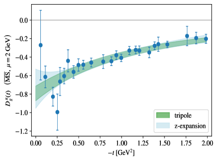
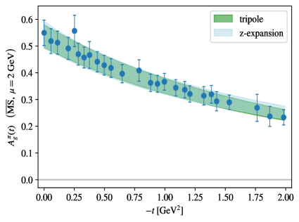
Figure 1: Agπ(t)subscriptsuperscript𝐴𝜋𝑔𝑡A^{\pi}_{g}(t) and Dgπ(t)subscriptsuperscript𝐷𝜋𝑔𝑡D^{\pi}_{g}(t) renormalized at μ=2GeV𝜇2GeV\mu=2~{}\text{GeV} in the MS¯¯MS\overline{\text{MS}} scheme. The bands correspond to the multipole form (Eq. (2)) with n=3𝑛3n=3 and the modified z-expansion (Eq. (3)) with kmax=2subscript𝑘max2k_{\text{max}}=2, with fit parameters shown in Tab. II.1.

Our lattice calculation yields the GFFs at a set of discrete values of the squared momentum transfer t𝑡t but, as discussed in Sec. III, subsequent extrapolations to the forward limit and derivations of densities and radii require models of the t𝑡t dependence of the GFFs. We consider two different ansätze, a multipole and a modification of the z-parameter expansion or “z-expansion” [76, 77]. The multipole form is defined as

Gn(t)=α(1t/Λ2)n,subscriptG𝑛𝑡𝛼superscript1𝑡superscriptΛ2𝑛\text{G}_{n}(t)=\frac{\alpha}{(1-t/\Lambda^{2})^{n}}, (2)

where α𝛼\alpha and ΛΛ\Lambda are free parameters and we set n=3𝑛3n=3 (tripole) in order for all the integrals that define the energy, pressure, and shear force densities discussed in Sec. III to converge. As introduced in Ref. [77], the modified z-expansion we consider is

Gz,n(t)=1(1t/Λ2)nk=0kmaxαk[z(t)]k,subscriptG𝑧𝑛𝑡1superscript1𝑡superscriptΛ2𝑛superscriptsubscript𝑘0subscript𝑘maxsubscript𝛼𝑘superscriptdelimited-[]𝑧𝑡𝑘\text{G}_{z,n}(t)=\frac{1}{(1-t/\Lambda^{2})^{n}}\sum_{k=0}^{k_{\text{max}}}\alpha_{k}[z(t)]^{k}\;, (3)

where

z(t)=tcutttcutt0tcutt+tcutt0,𝑧𝑡subscript𝑡cut𝑡subscript𝑡cutsubscript𝑡0subscript𝑡cut𝑡subscript𝑡cutsubscript𝑡0z(t)=\frac{\sqrt{t_{\text{cut}}-t}-\sqrt{t_{\text{cut}}-t_{0}}}{\sqrt{t_{\text{cut}}-t}+\sqrt{t_{\text{cut}}-t_{0}}}, (4)

αksubscript𝛼𝑘\alpha_{k} are free parameters, and ΛΛ\Lambda is constrained as described below. This functional form can be interpreted as a series of corrections to the envelope defined by the multipole form, which coincides with Eq. (3) when kmax=0subscript𝑘max0k_{\text{max}}=0. The multipole envelope is necessary for convergence of the density integrals discussed in Sec. III. Following Ref. [77], we set kmax=2subscript𝑘max2k_{\text{max}}=2, t0=tcut(11+(2GeV)2/tcut)subscript𝑡0subscript𝑡cut11superscript2GeV2subscript𝑡cutt_{0}=t_{\text{cut}}(1-\sqrt{1+(2\;\text{GeV})^{2}/t_{\text{cut}}}), and tcut=4mπ2subscript𝑡cut4superscriptsubscript𝑚𝜋2t_{\text{cut}}=4m_{\pi}^{2}, using mπ=450MeVsubscript𝑚𝜋450MeVm_{\pi}=450~{}\mathrm{MeV}. For each GFF, we use ΛΛ\Lambda obtained from the multipole fit to the same GFF as a prior for the parameter ΛΛ\Lambda in the z-expansion, retaining correlations between the prior and the data,222Compare with the discussion of “chained fitting” in Ref. [78]. thereby reducing the number of free parameters to prevent overfitting and explicitly enforcing the notion of the modified z-expansion as a correction to the multipole envelope. As detailed in Appendix A, we fit the models to bare GFFs and renormalize afterwards to circumvent the d’Agostini bias [79]; in this section we present the resulting renormalized parameters α𝛼\alpha and αksubscript𝛼𝑘\alpha_{k}.

II.1 Pion

The pion matrix element of the symmetric gluon or quark contribution to the energy-momentum tensor can be decomposed as

π(p)|Tiμν|π(p)bra𝜋superscript𝑝superscriptsubscript𝑇𝑖𝜇𝜈ket𝜋𝑝\displaystyle\bra{\pi(p^{\prime})}T_{i}^{\mu\nu}\ket{\pi(p)} =2PμPνAiπ(t)+2mπ2c¯iπ(t)gμνabsent2superscript𝑃𝜇superscript𝑃𝜈subscriptsuperscript𝐴𝜋𝑖𝑡2superscriptsubscript𝑚𝜋2subscriptsuperscript¯𝑐𝜋𝑖𝑡superscript𝑔𝜇𝜈\displaystyle=2P^{\mu}P^{\nu}A^{\pi}_{i}(t)+2m_{\pi}^{2}\bar{c}^{\pi}_{i}(t)g^{\mu\nu} (5)
+12(ΔμΔνgμνΔ2)Diπ(t)12superscriptΔ𝜇superscriptΔ𝜈superscript𝑔𝜇𝜈superscriptΔ2subscriptsuperscript𝐷𝜋𝑖𝑡\displaystyle~{}~{}+\frac{1}{2}(\Delta^{\mu}\Delta^{\nu}-g^{\mu\nu}\Delta^{2})D^{\pi}_{i}(t)
𝒪(π)μν[Aiπ(t),Diπ(t)]+trace,absentsubscriptsuperscript𝒪𝜇𝜈𝜋subscriptsuperscript𝐴𝜋𝑖𝑡subscriptsuperscript𝐷𝜋𝑖𝑡trace\displaystyle\equiv\mathcal{O}^{\mu\nu}_{(\pi)}[A^{\pi}_{i}(t),D^{\pi}_{i}(t)]+\text{trace}\;,

where i{q,g}𝑖𝑞𝑔i\in\{q,g\}, gμνsubscript𝑔𝜇𝜈g_{\mu\nu} is the Minkowski space-time metric, and we have defined the traceless piece 𝒪(π)μνsubscriptsuperscript𝒪𝜇𝜈𝜋\mathcal{O}^{\mu\nu}_{(\pi)} for later convenience. Aiπ(0)subscriptsuperscript𝐴𝜋𝑖0A^{\pi}_{i}(0) is the traceless contribution to the momentum fraction carried by the quarks or gluons and must satisfy Aπ(0)=iAiπ(0)=1superscript𝐴𝜋0subscript𝑖subscriptsuperscript𝐴𝜋𝑖01A^{\pi}(0)=\sum_{i}A^{\pi}_{i}(0)=1 because of Poincaré symmetry. Diπ(t)subscriptsuperscript𝐷𝜋𝑖𝑡D^{\pi}_{i}(t) is related to the mechanical properties of the pion. In the forward and chiral limits, the total Dπ(0)superscript𝐷𝜋0D^{\pi}(0), also called the D𝐷D-term or Druck term, is predicted to be 11-1 up to chiral-symmetry breaking effects [26, 80, 81]. c¯iπ(t)subscriptsuperscript¯𝑐𝜋𝑖𝑡\bar{c}^{\pi}_{i}(t) appears due to the nonconservation of the separate quark and gluon contributions and vanishes for the total EMT, i.e. c¯π(t)=c¯gπ(t)+qc¯qπ(t)=0superscript¯𝑐𝜋𝑡subscriptsuperscript¯𝑐𝜋𝑔𝑡subscript𝑞subscriptsuperscript¯𝑐𝜋𝑞𝑡0{\bar{c}^{\pi}(t)=\bar{c}^{\pi}_{g}(t)+\sum_{q}\bar{c}^{\pi}_{q}(t)=0}.

tripole α𝛼\alpha ΛΛ\Lambda [GeV] χ2/d.o.f.superscript𝜒2d.o.f.\chi^{2}/\text{d.o.f.}
Agπ(t)superscriptsubscript𝐴𝑔𝜋𝑡A_{g}^{\pi}(t) 0.537(45)0..537450.537(45) 2.561(43)2..561432.561(43) 0.90..90.9
Dgπ(t)superscriptsubscript𝐷𝑔𝜋𝑡D_{g}^{\pi}(t) 0.793(84)0..79384-0.793(84) 1.90(11)1..90111.90(11) 1.31..31.3
z-expansion α0subscript𝛼0\alpha_{0} α1subscript𝛼1\alpha_{1} α2subscript𝛼2\alpha_{2} χ2/\chi^{2}/d.o.f.
Agπ(t)superscriptsubscript𝐴𝑔𝜋𝑡A_{g}^{\pi}(t) 0.540(45)0..540450.540(45) 0.14(10)0..14100.14(10) 0.70(52)0..70520.70(52) 0.80..80.8
Dgπ(t)superscriptsubscript𝐷𝑔𝜋𝑡D_{g}^{\pi}(t) 0.793(70)0..79370-0.793(70) 0.21(75)0..21750.21(75) 2.0(7.3)2..07.32.0(7.3) 1.11..11.1
Table 2: Fit parameters of the multipole [Eq. (2)] with n=3𝑛3n=3 and the modified z-expansion [Eq. (3)] with kmax=2subscript𝑘max2k_{\text{max}}=2 and n=3𝑛3n=3 models for the t𝑡t dependence of the renormalized pion GFFs. For all GFFs, the parameter ΛΛ\Lambda of the z-expansion fit is consistent with the prior provided by the tripole fit and is thus not shown. The parameters α𝛼\alpha and αksubscript𝛼𝑘\alpha_{k} are renormalized at μ=2GeV𝜇2GeV\mu=2\;\text{GeV} after fitting the bare GFFs as described in Appendix A.5.
tripole z-expansion
Agπ(0)superscriptsubscript𝐴𝑔𝜋0A_{g}^{\pi}(0) 0.537(45)0..537450.537(45) 0.544(46)0..544460.544(46)
Dgπ(0)superscriptsubscript𝐷𝑔𝜋0D_{g}^{\pi}(0) 0.793(84)0..79384-0.793(84) 0.74(21)0..7421-0.74(21)
Table 3: The forward-limit values of the gluon momentum fraction and the gluon D𝐷D-term, obtained from the tripole and modified z-expansion fits to the pion GFFs, renormalized at μ=2GeV𝜇2GeV\mu=2\;\text{GeV} in the MS¯¯MS\overline{\text{MS}} scheme, with parameters shown in Table II.1.

Our results for the two renormalized traceless gluon GFFs of the pion, Agπ(t)subscriptsuperscript𝐴𝜋𝑔𝑡A^{\pi}_{g}(t) and Dgπ(t)subscriptsuperscript𝐷𝜋𝑔𝑡D^{\pi}_{g}(t), are shown in Fig. 1. The fit parameters for the two ansätze, Eqs. (2) and (3), are shown in Table II.1, and the predicted forward-limit gluon momentum fraction and D𝐷D-term are shown in Table II.1. We note that the sum of our gluon D𝐷D-term with the value Du+dπ(0)=0.264(32)superscriptsubscript𝐷𝑢𝑑𝜋00.26432D_{u+d}^{\pi}(0)=-0.264(32) (extrapolated to the physical pion mass) from Ref. [51] is statistically consistent with the chiral prediction, although this may be a coincidence that does not survive a chiral and continuum limit extrapolation.

II.2 Nucleon

For the nucleon, the GFFs of the symmetric gluon or quark parts of the EMT are defined by

N(p,σ)|Tiμν|N(p,σ)bra𝑁superscript𝑝superscript𝜎superscriptsubscript𝑇𝑖𝜇𝜈ket𝑁𝑝𝜎\displaystyle\bra{N(p^{\prime},\sigma^{\prime})}T_{i}^{\mu\nu}\ket{N(p,\sigma)} =\displaystyle=
u¯(𝐩,σ)[γ{μPν}AiN(t)+\displaystyle\bar{u}({\mathbf{p}}^{\prime},\sigma^{\prime})\bigg{[}\gamma_{\{\mu}P_{\nu\}}A^{N}_{i}(t)+ iP{μσν}ρΔρ2mNBiN(t)\displaystyle\frac{iP_{\{\mu}\sigma_{\nu\}\rho}\Delta^{\rho}}{2m_{N}}B^{N}_{i}(t)
+mNgμνc¯iN(t)+limit-fromsubscript𝑚𝑁subscript𝑔𝜇𝜈subscriptsuperscript¯𝑐𝑁𝑖𝑡\displaystyle+m_{N}g_{\mu\nu}\bar{c}^{N}_{i}(t)+ ΔμΔνgμνΔ24mNDiN(t)]u(𝐩,σ)\displaystyle\frac{\Delta_{\mu}\Delta_{\nu}-g_{\mu\nu}\Delta^{2}}{4m_{N}}D_{i}^{N}(t)\bigg{]}u({\mathbf{p}},\sigma)
u¯(𝐩,σ)𝒪(N)μν[\displaystyle\equiv\bar{u}({\mathbf{p}}^{\prime},\sigma^{\prime})\mathcal{O}^{\mu\nu}_{(N)}[ AiN(t),]u(𝐩,σ)+trace,\displaystyle A^{N}_{i}(t),...]u({\mathbf{p}},\sigma)+\text{trace}\;, (6)

where mNsubscript𝑚𝑁m_{N} denotes the nucleon mass, σμν=i2[γμ,γν]subscript𝜎𝜇𝜈𝑖2subscript𝛾𝜇subscript𝛾𝜈\sigma_{\mu\nu}=\frac{i}{2}[\gamma_{\mu},\gamma_{\nu}], and u(𝐩,σ)𝑢𝐩𝜎u({\mathbf{p}},\sigma) is the Dirac spinor, which satisfies

σu(𝐩,σ)u¯(𝐩,σ)=p+mN,subscript𝜎𝑢𝐩𝜎¯𝑢𝐩𝜎cancel𝑝subscript𝑚𝑁\sum_{\sigma}u({\mathbf{p}},\sigma)\bar{u}({\mathbf{p}},\sigma)=\cancel{p}+m_{N}\;, (7)

where σ{1/2,+1/2}𝜎1212\sigma\in\{-1/2,+1/2\}. Equation II.2 is often expressed in terms of the form factor JiN(t)=(AiN(t)+BiN(t))/2subscriptsuperscript𝐽𝑁𝑖𝑡subscriptsuperscript𝐴𝑁𝑖𝑡subscriptsuperscript𝐵𝑁𝑖𝑡2J^{N}_{i}(t)=(A^{N}_{i}(t)+B^{N}_{i}(t))/2 instead of BiN(t)subscriptsuperscript𝐵𝑁𝑖𝑡B^{N}_{i}(t), where the total JN(0)=1/2superscript𝐽𝑁012J^{N}(0)=1/2 is the spin of the nucleon. As for the total GFFs for spin-0 states, AN(0)=1superscript𝐴𝑁01A^{N}(0)=1 and c¯N(t)=0superscript¯𝑐𝑁𝑡0\bar{c}^{N}(t)=0 for the GFFs of spin-1/2 states. The new form factor BN(t)superscript𝐵𝑁𝑡B^{N}(t) that appears for hadrons of spin >0absent0>0 must obey BN(0)=0superscript𝐵𝑁00B^{N}(0)=0 due to the vanishing of the anomalous gravitomagnetic moment of spin-1/2 fermions [82, 5, 11, 83, 84, 85, 86, 87, 88]. The are no a priori restrictions on the D𝐷D-term of a spin-1/2 hadron, but for a free fermion DN(0)=0superscript𝐷𝑁00D^{N}(0)=0 [89].

Refer to caption
(a)
Refer to caption
(b)
Refer to caption
(c)
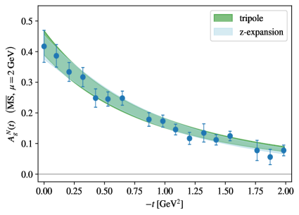
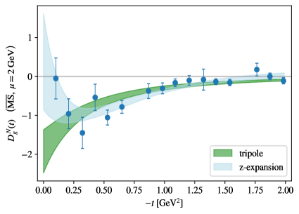
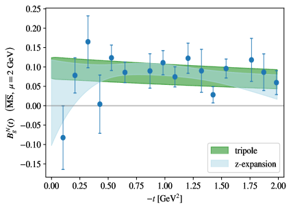
Figure 2: AgN(t)subscriptsuperscript𝐴𝑁𝑔𝑡A^{N}_{g}(t) (a), DgN(t)subscriptsuperscript𝐷𝑁𝑔𝑡D^{N}_{g}(t) (b), and BgN(t)subscriptsuperscript𝐵𝑁𝑔𝑡B^{N}_{g}(t) (c), renormalized at μ=2GeV𝜇2GeV\mu=2~{}\text{GeV} in the MS¯¯MS\overline{\text{MS}} scheme. The bands correspond to the multipole form [Eq. (2)] with n=3𝑛3n=3 and the modified z-expansion [Eq. (3)] with kmax=2subscript𝑘max2k_{\text{max}}=2, with fit parameters shown in Table II.2.


tripole α𝛼\alpha ΛΛ\Lambda [GeV] χ2/\chi^{2}/d.o.f.
AgN(t)superscriptsubscript𝐴𝑔𝑁𝑡A_{g}^{N}(t) 0.429(39)0..429390.429(39) 1.641(43)1..641431.641(43) 1.11..11.1
BgN(t)superscriptsubscript𝐵𝑔𝑁𝑡B_{g}^{N}(t) 0.097(26)0..097260.097(26) 4.0(2.5)4..02.54.0(2.5) 1.41..41.4
DgN(t)superscriptsubscript𝐷𝑔𝑁𝑡D_{g}^{N}(t) 1.93(53)1..9353-1.93(53) 1.07(12)1..07121.07(12) 2.02..02.0
z-expansion α0subscript𝛼0\alpha_{0} α1subscript𝛼1\alpha_{1} α2subscript𝛼2\alpha_{2} χ2/\chi^{2}/d.o.f.
AgN(t)superscriptsubscript𝐴𝑔𝑁𝑡A_{g}^{N}(t) 0.426(38)0..426380.426(38) 0.22(22)0..2222-0.22(22) 1.2(1.2)1..21.2-1.2(1.2) 0.90..90.9
BgN(t)superscriptsubscript𝐵𝑔𝑁𝑡B_{g}^{N}(t) 0.108(16)0..108160.108(16) 0.19(20)0..1920-0.19(20) 2.9(3.2)2..93.2-2.9(3.2) 1.11..11.1
DgN(t)superscriptsubscript𝐷𝑔𝑁𝑡D_{g}^{N}(t) 2.09(35)2..0935-2.09(35) 18.0(7.9)18..07.918.0(7.9) 132(58)formulae-sequence13258132(58) 1.01..01.0
Table 4: Fit parameters of the multipole [Eq. (2)] with n=3𝑛3n=3 and the modified z-expansion [Eq. (3)] with kmax=2subscript𝑘max2k_{\text{max}}=2 and n=3𝑛3n=3 models for the t𝑡t dependence of the renormalized nucleon GFFs. For all GFFs, the parameter ΛΛ\Lambda of the z-expansion fit is consistent with the prior provided by the tripole fit and is thus not shown. The parameters α𝛼\alpha and αksubscript𝛼𝑘\alpha_{k} are renormalized at μ=2GeV𝜇2GeV\mu=2\;\text{GeV} after fitting the bare GFFs as described in Appendix A.5.
tripole z-expansion
AgN(0)superscriptsubscript𝐴𝑔𝑁0A_{g}^{N}(0) 0.429(39)0..429390.429(39) 0.414(40)0..414400.414(40)
DgN(0)superscriptsubscript𝐷𝑔𝑁0D_{g}^{N}(0) 1.93(53)1..9353-1.93(53) 0.4(1.2)0..41.20.4(1.2)
JgN(0)superscriptsubscript𝐽𝑔𝑁0J_{g}^{N}(0) 0.263(26)0..263260.263(26) 0.211(57)0..211570.211(57)
Table 5: The forward-limit values of the gluon contributions to the momentum fraction, D𝐷D-term, and angular momentum of the nucleon, obtained from the tripole and modified z-expansion fits of the nucleon GFFs renormalized at μ=2GeV𝜇2GeV{\mu=2\;\text{GeV}} in the MS¯¯MS\overline{\text{MS}} scheme, with parameters shown in Table II.2.

Our results for the three renormalized traceless gluon GFFs of the nucleon are shown in Fig. 1a, the tripole and modified z-expansion fit parameters are shown in Table II.2, and the predictions for the forward-limit gluon contributions to the momentum fraction, D𝐷D-term, and angular momentum are shown in Table II.2. Note that the increase order-by-order of the parameters in the modified z-expansion fit for the D𝐷D-term are not of concern, as we consider here a modification of the standard z-expansion for which the guarantees of convergence for the standard form do not apply.

These results are based on a superset of the data presented in Ref. [60], including a larger number of sources per configuration and all four nucleon polarization channels, rather than only the two spin-conserving ones. The additional data allows a nonzero functional fit for BgN(t)superscriptsubscript𝐵𝑔𝑁𝑡B_{g}^{N}(t) to be resolved. Additionally, the behavior of AgN(t)superscriptsubscript𝐴𝑔𝑁𝑡A_{g}^{N}(t) and DgN(t)superscriptsubscript𝐷𝑔𝑁𝑡D_{g}^{N}(t) in the lower half of the t𝑡-t region studied is shifted slightly compared to what was found in Ref. [60]. These updated results show a qualitative difference between the low-|t|𝑡|t| behavior of the model obtained for DgN(t)subscriptsuperscript𝐷𝑁𝑔𝑡D^{N}_{g}(t) with the tripole functional form (that is by definition monotonic), and the modified z-expansion fit (that is allowed to be nonmonotonic). In general, monotonically increasing behavior is universally expected for the total D𝐷D-term of any stable mechanical system [90]; however, no such prediction exists for the individual quark and gluon contributions. It is not clear whether the suppression of the lowest-|t|𝑡|t| point of DgN(t)subscriptsuperscript𝐷𝑁𝑔𝑡D^{N}_{g}(t) is physical or due to a statistical fluctuation or unquantified systematic uncertainty. If physical, it would imply a qualitatively different t𝑡t dependence of the gluon GFFs compared with that typically assumed for the quark GFFs, and suggest that the multipole functional form often used by default for these quantities is not a good model at low |t|𝑡|t|. If the first data point is considered an outlier and excluded from the z-expansion fit, the resulting error bands do not exclude nonmonotonicity but encompass both monotonic and nonmonotonic forms.

Our predictions for AgN(0)superscriptsubscript𝐴𝑔𝑁0A_{g}^{N}(0) and JgN(0)superscriptsubscript𝐽𝑔𝑁0J_{g}^{N}(0) are statistically consistent with the equivalent quantities found in a lattice QCD calculation at quark masses corresponding to the physical value of the pion mass [56].

II.3 ρ𝜌\rho Meson

Following the conventions of Ref. [91], the matrix elements of the gluon or quark contribution to the symmetric EMT for the ρ𝜌\rho meson can be decomposed as

ρ(p’,λ’)—Tiμνρ(p,λ)⟩=ϵα*(p’,λ’) ϵα(p,λ) [ 2PμPν(-gααAρ0,i(t) + PαPαmρ2Aρ1,i(t))+ 12(ΔμΔν-gμνΔ2) (gααDρ0,i(t)+ PαPαmρ2Dρ1,i(t))+4[P{μgν}αPα+P{μgν}αPα]Jρi(t) +[gα{μgν}αΔ2- 2gα’{μΔν}Pα+2gα{μΔν}Pα-4gμνPαPα]Eiρ(t) +[2gα{μgν}α-12gααgμν]mρ2¯fiρ(t) +gμν[gααmρ2¯ci0,ρ(t)+PαPα¯ci1,ρ(t)] ]ϵα*(p’,λ’) ϵα(p,λ) Oαμνα(ρ)[A0,iρ(t), A1,iρ(t),D0,iρ(t),D1,iρ(t), Jiρ(t),Eiρ(t),¯fiρ(t)] + trace,

(8)

where mρsubscript𝑚𝜌m_{\rho} denotes the mass of the ρ𝜌\rho meson, and ϵα(𝐩,λ)subscriptitalic-ϵ𝛼𝐩𝜆\epsilon_{\alpha}({\mathbf{p}},\lambda) is the polarization 4-vector for a massive spin-1 particle, which satisfies

λϵα(𝐩,λ)ϵβ(𝐩,λ)=gαβ+pαpβmρ2Λαβ(ρ)(𝐩)subscript𝜆subscriptitalic-ϵ𝛼𝐩𝜆subscriptitalic-ϵ𝛽𝐩𝜆subscript𝑔𝛼𝛽subscript𝑝𝛼subscript𝑝𝛽superscriptsubscript𝑚𝜌2superscriptsubscriptΛ𝛼𝛽𝜌𝐩\sum_{\lambda}\epsilon_{\alpha}({\mathbf{p}},\lambda)\epsilon_{\beta}({\mathbf{p}},\lambda)=-g_{\alpha\beta}+\frac{p_{\alpha}p_{\beta}}{m_{\rho}^{2}}\equiv\Lambda_{\alpha\beta}^{(\rho)}({\mathbf{p}}) (9)

with λ{1,0,1}𝜆101\lambda\in\{1,0,-1\}. Note that the subscript ρ𝜌\rho in mρsubscript𝑚𝜌m_{\rho} and the superscript ρ𝜌\rho in the GFFs such as A0,iρ(t)superscriptsubscript𝐴0𝑖𝜌𝑡A_{0,i}^{\rho}(t) is a label for the ρ𝜌\rho meson and not a Lorentz index.

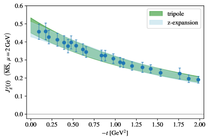
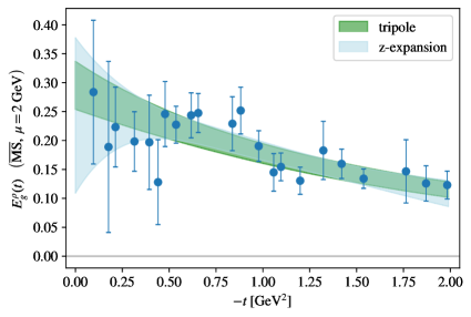
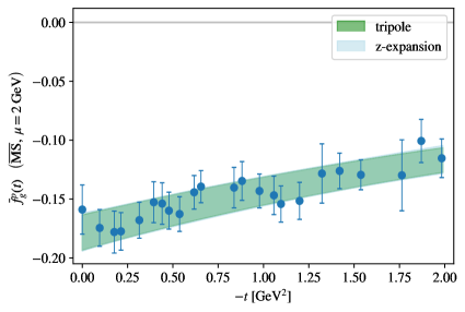
The momentum sum rule constrains the total momentum fraction to be Aρ(0)A0ρ(0)=1superscript𝐴𝜌0superscriptsubscript𝐴0𝜌01A^{\rho}(0)\equiv A_{0}^{\rho}(0)=1, and the forward-limit angular momentum must be equal to the spin of the hadron, i.e., Jρ(0)=1superscript𝐽𝜌01J^{\rho}(0)=1. The interpretation of the D𝐷D-term of the ρ𝜌\rho meson is more complicated than those of the pion and the nucleon, since there are three such terms [91, 48], one of monopole and two of quadrupole order, corresponding to frame-dependent linear combinations of D0ρ(0)superscriptsubscript𝐷0𝜌0D_{0}^{\rho}(0), D1ρ(0)superscriptsubscript𝐷1𝜌0D_{1}^{\rho}(0), and Eρ(0)superscript𝐸𝜌0E^{\rho}(0). Here we focus on the forward limit of the form factor that is the coefficient of the same Lorentz structure corresponding to the D𝐷D-term GFFs of the nucleon and pion, namely Dρ(0)D0ρ(0)superscript𝐷𝜌0superscriptsubscript𝐷0𝜌0D^{\rho}(0)\equiv-D_{0}^{\rho}(0), which is unconstrained from theory. There are two GFFs that arise from the trace of the EMT, c¯i1,ρ(t)superscriptsubscript¯𝑐𝑖1𝜌𝑡\bar{c}_{i}^{1,\rho}(t) and c¯i2,ρ(t)superscriptsubscript¯𝑐𝑖2𝜌𝑡\bar{c}_{i}^{2,\rho}(t), and their contribution to the total EMT must be equal to zero. In contrast to the pion and the nucleon GFF decompositions, the traceless piece of the EMT matrix element for hadrons of spin-1 gives rise to a nonconserved GFF, f¯iρ(t)superscriptsubscript¯𝑓𝑖𝜌𝑡\bar{f}_{i}^{\rho}(t), which we can access in our calculation and vanishes when summed over the quark and gluon contributions.

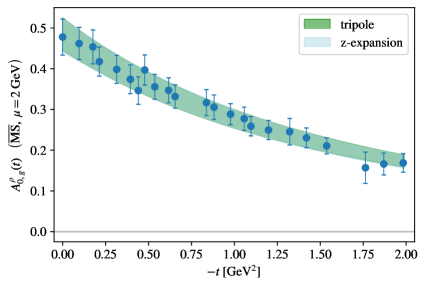
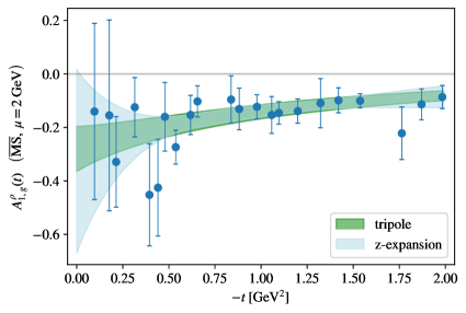
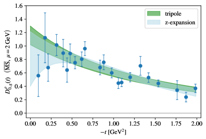
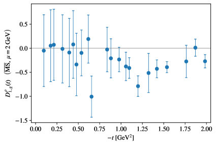
Our results for the seven renormalized traceless gluon GFFs are shown in Fig. 2a. Model fit parameters are tabulated in Table II.3, excluding for the GFF D1,gρ(t)superscriptsubscript𝐷1𝑔𝜌𝑡D_{1,g}^{\rho}(t), which is not well described by either model ansatz. The conserved gluon predictions of these quantities are presented in Table II.3.

We find that approximately half of the angular momentum of the ρ𝜌\rho meson is carried by gluons. Interestingly, the NJL model [33] predicts that half is carried by the quark spin. Just as in the nucleon case, we find a significant difference between the forward limit of the D𝐷D form factor resulting from the tripole fit and the z-expansion (see Table II.3) which can be traced to the difference of the two fits in the low momentum region of D0,gρ(t)superscriptsubscript𝐷0𝑔𝜌𝑡D_{0,g}^{\rho}(t) as seen in Fig. 2a(c). Here the first data point again suggests nonmonotonic behavior that cannot be captured by a multipole form, but it is unclear whether this is a physical effect or due to a statistical fluctuation or underestimated systematic uncertainty. In Ref. [48], the total D0ρ(t)superscriptsubscript𝐷0𝜌𝑡D_{0}^{\rho}(t) from the light-front constituent quark model was found to be nonmonotonic, in contrast with the prediction from the NJL model [33].

tripole α𝛼\alpha ΛΛ\Lambda [GeV] χ2/\chi^{2}/d.o.f.
A0,gρ(t)superscriptsubscript𝐴0𝑔𝜌𝑡A_{0,g}^{\rho}(t) 0.485(41)0..485410.485(41) 2.205(41)2..205412.205(41) 0.80..80.8
A1,gρ(t)superscriptsubscript𝐴1𝑔𝜌𝑡A_{1,g}^{\rho}(t) 0.281(84)0..28184-0.281(84) 1.97(43)1..97431.97(43) 0.50..50.5
D0,gρ(t)superscriptsubscript𝐷0𝑔𝜌𝑡D_{0,g}^{\rho}(t) 1.16(14)1..16141.16(14) 2.01(14)2..01142.01(14) 1.91..91.9
Jgρ(t)superscriptsubscript𝐽𝑔𝜌𝑡J_{g}^{\rho}(t) 0.491(42)0..491420.491(42) 2.327(44)2..327442.327(44) 0.60..60.6
Egρ(t)superscriptsubscript𝐸𝑔𝜌𝑡E_{g}^{\rho}(t) 0.295(41)0..295410.295(41) 2.33(25)2..33252.33(25) 0.70..70.7
f¯gρ(t)superscriptsubscript¯𝑓𝑔𝜌𝑡\bar{f}_{g}^{\rho}(t) 0.178(15)0..17815-0.178(15) 3.63(22)3..63223.63(22) 0.80..80.8
z-expansion α0subscript𝛼0\alpha_{0} α1subscript𝛼1\alpha_{1} α2subscript𝛼2\alpha_{2} χ2/\chi^{2}/d.o.f.
A0,gρ(t)superscriptsubscript𝐴0𝑔𝜌𝑡A_{0,g}^{\rho}(t) 0.485(41)0..485410.485(41) 0.04(11)0..0411-0.04(11) 0.23(66)0..2366-0.23(66) 0.70..70.7
A1,gρ(t)superscriptsubscript𝐴1𝑔𝜌𝑡A_{1,g}^{\rho}(t) 0.276(42)0..27642-0.276(42) 0.10(71)0..1071-0.10(71) 2(11)formulae-sequence211-2(11) 0.50..50.5
D0,gρ(t)superscriptsubscript𝐷0𝑔𝜌𝑡D_{0,g}^{\rho}(t) 1.19(11)1..19111.19(11) 0.86(85)0..8685-0.86(85) 12(12)formulae-sequence1212-12(12) 1.61..61.6
Jgρ(t)superscriptsubscript𝐽𝑔𝜌𝑡J_{g}^{\rho}(t) 0.494(42)0..494420.494(42) 0.105(69)0..10569-0.105(69) 1.01(66)1..0166-1.01(66) 0.40..40.4
Egρ(t)superscriptsubscript𝐸𝑔𝜌𝑡E_{g}^{\rho}(t) 0.301(29)0..301290.301(29) 0.11(24)0..1124-0.11(24) 1.7(3.8)1..73.8-1.7(3.8) 0.60..60.6
f¯gρ(t)superscriptsubscript¯𝑓𝑔𝜌𝑡\bar{f}_{g}^{\rho}(t) 0.179(15)0..17915-0.179(15) 0.005(54)0..005540.005(54) 0.04(37)0..04370.04(37) 0.70..70.7
Table 6: Fit parameters of the multipole [Eq. (2)] with n=3𝑛3n=3 and the modified z-expansion [Eq. (3)] with kmax=2subscript𝑘max2k_{\text{max}}=2 and n=3𝑛3n=3 models for the t𝑡t dependence of the renormalized ρ𝜌\rho GFFs. The signal for D1,gρ(t)superscriptsubscript𝐷1𝑔𝜌𝑡D_{1,g}^{\rho}(t) is not well described by either functional form and therefore no fit is shown. For all GFFs that have been fit, the parameter ΛΛ\Lambda of the z-expansion fit is consistent with the prior provided by the tripole fit and is thus not shown. The parameters α𝛼\alpha and αksubscript𝛼𝑘\alpha_{k} are renormalized at μ=2GeV𝜇2GeV\mu=2\;\text{GeV} after fitting the bare GFFs as described in Appendix A.5.
tripole z-expansion
Agρ(0)superscriptsubscript𝐴𝑔𝜌0A_{g}^{\rho}(0) 0.485(41)0..485410.485(41) 0.482(42)0..482420.482(42)
Dgρ(0)superscriptsubscript𝐷𝑔𝜌0D_{g}^{\rho}(0) 1.16(14)1..1614-1.16(14) 0.81(38)0..8138-0.81(38)
Jgρ(0)superscriptsubscript𝐽𝑔𝜌0J_{g}^{\rho}(0) 0.491(42)0..491420.491(42) 0.469(42)0..469420.469(42)
Table 7: The forward-limit values of the conserved gluon contribution to the momentum fraction, D𝐷D form factor, and angular momentum of the ρ𝜌\rho meson, with definitions provided in the text. The values are obtained from the tripole and modified z-expansion fits of the ρ𝜌\rho GFFs, renormalized at μ=2GeV𝜇2GeV{\mu=2\;\text{GeV}} in the MS¯¯MS\overline{\text{MS}} scheme, with parameters shown in Table II.3.
Refer to caption
(a)
Refer to caption
(b)
Refer to caption
(c)
Refer to caption
(d)
Refer to caption
(e)
Refer to caption
(f)
Refer to caption
(g)
Figure 3: A0,gρ(t)subscriptsuperscript𝐴𝜌0𝑔𝑡A^{\rho}_{0,g}(t) (a), A1,gρ(t)subscriptsuperscript𝐴𝜌1𝑔𝑡A^{\rho}_{1,g}(t) (b), D0,gρ(t)subscriptsuperscript𝐷𝜌0𝑔𝑡D^{\rho}_{0,g}(t) (c), D1,gρ(t)subscriptsuperscript𝐷𝜌1𝑔𝑡D^{\rho}_{1,g}(t) (d), Jgρ(t)subscriptsuperscript𝐽𝜌𝑔𝑡J^{\rho}_{g}(t) (e), Egρ(t)subscriptsuperscript𝐸𝜌𝑔𝑡E^{\rho}_{g}(t) (f), and f¯gρ(t)subscriptsuperscript¯𝑓𝜌𝑔𝑡\overline{f}^{\rho}_{g}(t) (g), renormalized at μ=2GeV𝜇2GeV\mu=2\;\text{GeV} in the MS¯¯MS\overline{\text{MS}} scheme. The bands correspond to the multipole form [Eq. (2)] with n=3𝑛3n=3 and the modified z-expansion [Eq. (3)] with kmax=2subscript𝑘max2k_{\text{max}}=2, with fit parameters shown in Table II.3. No fit is shown for D1g(t)superscriptsubscript𝐷1𝑔𝑡D_{1}^{g}(t) because the corresponding data is not well described by either functional form.


II.4 ΔΔ\Delta Baryon

tripole α𝛼\alpha ΛΛ\Lambda [GeV] χ2/\chi^{2}/d.o.f.
F10Δ,g(t)superscriptsubscript𝐹10Δ𝑔𝑡F_{10}^{\Delta,g}(t) 0.393(36)0..393360.393(36) 1.788(66)1..788661.788(66) 1.21..21.2
F20Δ,g(t)superscriptsubscript𝐹20Δ𝑔𝑡F_{20}^{\Delta,g}(t) 1.80(69)1..8069-1.80(69) 1.10(17)1..10171.10(17) 2.32..32.3
F40Δ,g(t)superscriptsubscript𝐹40Δ𝑔𝑡F_{40}^{\Delta,g}(t) 0.587(78)0..587780.587(78) 1.421(78)1..421781.421(78) 2.02..02.0
F60Δ,g(t)superscriptsubscript𝐹60Δ𝑔𝑡F_{60}^{\Delta,g}(t) 0.0492(89)0..0492890.0492(89) 2.26(38)2..26382.26(38) 2.12..12.1
z-expansion α0subscript𝛼0\alpha_{0} α1subscript𝛼1\alpha_{1} α2subscript𝛼2\alpha_{2} χ2/\chi^{2}/d.o.f.
F10Δ,g(t)superscriptsubscript𝐹10Δ𝑔𝑡F_{10}^{\Delta,g}(t) 0.395(35)0..395350.395(35) 0.19(21)0..1921-0.19(21) 1.2(1.4)1..21.4-1.2(1.4) 1.01..01.0
F20Δ,g(t)superscriptsubscript𝐹20Δ𝑔𝑡F_{20}^{\Delta,g}(t) 2.36(42)2..3642-2.36(42) 18.8(8.4)18..88.418.8(8.4) 153(68)formulae-sequence15368153(68) 1.31..31.3
F40Δ,g(t)superscriptsubscript𝐹40Δ𝑔𝑡F_{40}^{\Delta,g}(t) 0.623(62)0..623620.623(62) 0.56(49)0..5649-0.56(49) 7.0(6.0)7..06.0-7.0(6.0) 1.61..61.6
F60Δ,g(t)superscriptsubscript𝐹60Δ𝑔𝑡F_{60}^{\Delta,g}(t) 0.0554(69)0..0554690.0554(69) 0.154(97)0..15497-0.154(97) 1.49(93)1..4993-1.49(93) 1.51..51.5
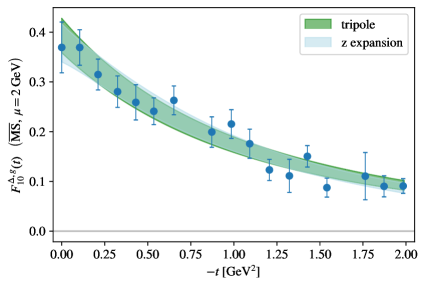
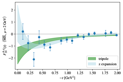
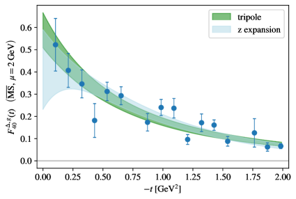
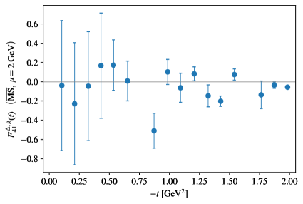
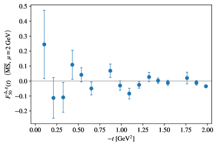
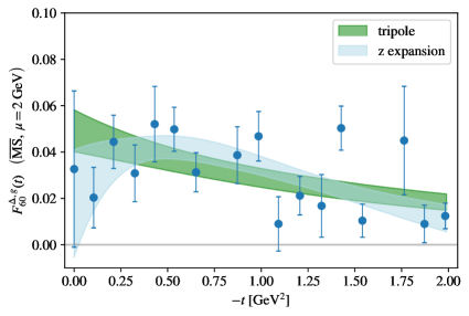
Table 8: Fit parameters of the multipole [Eq. (2)] with n=3𝑛3n=3 and the modified z-expansion [Eq. (3)] with kmax=2subscript𝑘max2k_{\text{max}}=2 and n=3𝑛3n=3 models for the t𝑡t dependence of the renormalized ΔΔ\Delta GFFs. Only four of the eight GFFs are fit, as the others are not resolved from zero as seen in Fig. 3a. For all GFFs that have been fit, the parameter ΛΛ\Lambda of the z-expansion fit is consistent with the prior provided by the tripole fit and is thus not shown. The parameters α𝛼\alpha and αksubscript𝛼𝑘\alpha_{k} are renormalized at μ=2GeV𝜇2GeV\mu=2\;\text{GeV} after fitting the bare GFFs as described in Appendix A.5.
tripole z-expansion
AgΔ(0)subscriptsuperscript𝐴Δ𝑔0A^{\Delta}_{g}(0) 0.393(36)0..393360.393(36) 0.378(38)0..378380.378(38)
DgΔ(0)subscriptsuperscript𝐷Δ𝑔0D^{\Delta}_{g}(0) 1.80(69)1..8069-1.80(69) 0.9(1.5)0..91.50.9(1.5)
JgΔ(0)subscriptsuperscript𝐽Δ𝑔0J^{\Delta}_{g}(0) 0.588(78)0..588780.588(78) 0.41(18)0..41180.41(18)
Table 9: The forward-limit values of the conserved gluon contribution to the momentum fraction, D𝐷D form factor, and angular momentum of the ΔΔ\Delta baryon, obtained from the tripole and modified z-expansion fits of the ΔΔ\Delta GFFs, renormalized at μ=2GeV𝜇2GeV\mu=2\;\text{GeV} in the MS¯¯MS\overline{\text{MS}} scheme, with parameters shown in Table II.4.
Refer to caption
(a)
Refer to caption
(b)
Refer to caption
(c)
Refer to caption
(d)
Refer to caption
(e)
Refer to caption
(f)
Refer to caption
(g)
Refer to caption
(h)
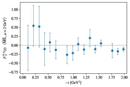
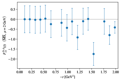
Figure 4: F10Δ,g(t)subscriptsuperscript𝐹Δ𝑔10𝑡F^{\Delta,g}_{10}(t) (a), F11Δ,g(t)subscriptsuperscript𝐹Δ𝑔11𝑡F^{\Delta,g}_{11}(t) (b), F20Δ,g(t)subscriptsuperscript𝐹Δ𝑔20𝑡F^{\Delta,g}_{20}(t) (c), F21Δ,g(t)subscriptsuperscript𝐹Δ𝑔21𝑡F^{\Delta,g}_{21}(t) (d), F40Δ,g(t)subscriptsuperscript𝐹Δ𝑔40𝑡F^{\Delta,g}_{40}(t) (e), F41Δ,g(t)subscriptsuperscript𝐹Δ𝑔41𝑡F^{\Delta,g}_{41}(t) (f), F50Δ,g(t)subscriptsuperscript𝐹Δ𝑔50𝑡F^{\Delta,g}_{50}(t) (g), F60Δ,g(t)subscriptsuperscript𝐹Δ𝑔60𝑡F^{\Delta,g}_{60}(t) (h), renormalized at μ=2GeV𝜇2GeV\mu=2~{}\text{GeV} in the MS¯¯MS\overline{\text{MS}} scheme. The bands correspond to the multipole form [Eq. (2)] with n=3𝑛3n=3 and the modified z-expansion [Eq. (3)] with kmax=2subscript𝑘max2k_{\text{max}}=2, with fit parameters shown in Table II.4. No fit is shown for the four GFFs that are not resolved from zero.


For the ΔΔ\Delta baryon, the matrix element of the quark or gluon symmetric EMT can be decomposed as [37]

⟨Δ(p’,ξ’)—Tiμν—Δ(p,ξ)⟩= ¯uα(p’,ξ’)[ PμPνmΔ(-gααFΔ,i10(t) + ΔαΔα2mΔ2FΔ,i11(t))+ ΔμΔν-gμνΔ24mΔ(-gααFΔ,i20(t)+ΔαΔα2mΔ2FΔ,i21(t))+mΔgμν(-gααFΔ,i30(t) +ΔαΔα2mΔ2FΔ,i31(t))+i P{μσν}ρΔρmΔ(-gααFΔ,i40(t)+ ΔαΔα2mΔ2FΔ,i41(t))+2mΔ{μgν}{αΔα}-gμνΔαΔα-gα’{μgν}αΔ2) FΔ,i50(t) -2 gα’{μgν}αmΔFΔ,i60(t) ] uα(p,ξ) ≡¯uα(p’,ξ’) O(Δ)αμνα[FΔ,i10(t),FΔ,i11(t),FΔ,i20(t),FΔ,i21(t),FΔ,i40(t),FΔ,i41(t),FΔ,i50(t),FΔ,i60(t)]uα(p,ξ) + trace  ,

(10)

where mΔsubscript𝑚Δm_{\Delta} denotes the mass of the ΔΔ\Delta baryon, and uα(𝐩,ξ)subscript𝑢𝛼𝐩𝜉u_{\alpha}({\mathbf{p}},\xi) is the Rarita-Schwinger spin-vector satisfying

ξuσ(𝐩,ξ)u¯τ(𝐩,ξ)=p+mΔ2mΔ(gστ12γσγτ2pσpτ3mΔ2+pσγτpτγσ3mΔ)Λστ(Δ)(p)subscript𝜉subscript𝑢𝜎𝐩𝜉subscript¯𝑢𝜏𝐩𝜉cancel𝑝subscript𝑚Δ2subscript𝑚Δsubscript𝑔𝜎𝜏12subscript𝛾𝜎subscript𝛾𝜏2subscript𝑝𝜎subscript𝑝𝜏3superscriptsubscript𝑚Δ2subscript𝑝𝜎subscript𝛾𝜏subscript𝑝𝜏subscript𝛾𝜎3subscript𝑚ΔsubscriptsuperscriptΛΔ𝜎𝜏𝑝\begin{split}\sum_{\xi}u_{\sigma}({\mathbf{p}},\xi)\bar{u}_{\tau}({\mathbf{p}},\xi)&\\ =-\frac{\cancel{p}+m_{\Delta}}{2m_{\Delta}}\bigg{(}g_{\sigma\tau}-&\frac{1}{2}\gamma_{\sigma}\gamma_{\tau}-\frac{2p_{\sigma}p_{\tau}}{3m_{\Delta}^{2}}+\frac{p_{\sigma}\gamma_{\tau}-p_{\tau}\gamma_{\sigma}}{3m_{\Delta}}\bigg{)}\\ \equiv\Lambda^{(\Delta)}_{\sigma\tau}(p)\qquad\qquad&\end{split} (11)

with ξ{3/2,1/2,1/2,3/2}𝜉32121232\xi\in\{3/2,1/2,-1/2,-3/2\}.

The total momentum fraction AΔ(0)F10Δ(0)superscript𝐴Δ0subscriptsuperscript𝐹Δ100A^{\Delta}(0)\equiv F^{\Delta}_{10}(0) is constrained to equal 111. As with the ρ𝜌\rho, there are three total D𝐷D-terms of different order and we again focus our discussion on the form factor that is the coefficient of the same Lorentz structure as the nucleon and pion D𝐷D-terms, namely DΔ(0)F20Δ(0)superscript𝐷Δ0subscriptsuperscript𝐹Δ200D^{\Delta}(0)\equiv F^{\Delta}_{20}(0). The total forward-limit angular momentum, JΔ(0)=F40Δ(0)superscript𝐽Δ0subscriptsuperscript𝐹Δ400{J^{\Delta}(0)=F^{\Delta}_{40}(0)}, is constrained to be equal to 3/2323/2 [37]. Just as in the case of the ρ𝜌\rho meson, there are nonconserved GFFs related to the trace piece, F30Δ,i(t)superscriptsubscript𝐹30Δ𝑖𝑡F_{30}^{\Delta,i}(t) and F31Δ,i(t)superscriptsubscript𝐹31Δ𝑖𝑡F_{31}^{\Delta,i}(t), that we do not have access to in this calculation, and one nonconserved GFF F60Δ,i(t)superscriptsubscript𝐹60Δ𝑖𝑡F_{60}^{\Delta,i}(t), that arises from the traceless EMT and that we are able to constrain.

Our results for the eight renormalized traceless gluon GFFs of the ΔΔ\Delta baryon are shown in Fig. 3a. Only four of them are resolved from zero, and their fit parameters are shown in Table II.4. The conserved gluon contributions to the forward limit quantities obtained from the tripole and z𝑧z-expansion fits are shown in Table II.4.

III DENSITIES AND RADII FROM GFFs

In the decomposition of the matrix element h(p,s)|Tiμν|h(p,s)brasuperscript𝑝superscript𝑠superscriptsubscript𝑇𝑖𝜇𝜈ket𝑝𝑠\bra{h(p^{\prime},s^{\prime})}T_{i}^{\mu\nu}\ket{h(p,s)}, the GFFs are Lorentz scalars but their coefficients depend on the reference frame. The spatial energy, pressure, and shear force densities of hadrons are related to Fourier transforms of the momentum space matrix elements, and therefore are also frame dependent. In this work we consider these densities in two frames, namely the Breit frame and the infinite momentum frame.

Breit frame (BF).—The “brick-wall” frame in which there is no energy transfer to the system, Δ0=0superscriptΔ00\Delta^{0}=0, and additionally 𝐏=0𝐏0{\mathbf{P}}=0. This is the frame traditionally used to define spatial distributions, such as the charge distribution in terms of the electromagnetic form factors [92]. The equivalent 3D density for the EMT in the BF (the BF3 density) is

Ti,BF3μν(r)=d3Δei𝚫𝐫2P0(2π)3h(p,s)|Tiμν|h(p,s)|𝐏=0,T^{\mu\nu}_{i,\text{BF3}}(r)=\int\frac{d^{3}\Delta e^{-i{\mathbf{\Delta}}\cdot{\mathbf{r}}}}{{2P^{0}}(2\pi)^{3}}\bra{h(p^{\prime},s^{\prime})}T_{i}^{\mu\nu}\ket{h(p,s)}\bigr{\rvert}_{{\mathbf{P}}=0}\;, (12)

where P0=mh2+𝚫2/4superscript𝑃0superscriptsubscript𝑚2superscript𝚫24P^{0}=\sqrt{m_{h}^{2}+{\mathbf{\Delta}}^{2}/4}, while in a 2D plane, the (BF2) density is equal to

Ti,BF2μν(r)=d2Δei𝚫𝐫2P0(2π)2h(p,s)|Tiμν|h(p,s|𝐏=0.T^{\mu\nu}_{i,\text{BF2}}(r)=\int\frac{d^{2}\Delta_{{\!\bot\!}}e^{-i{\mathbf{\Delta}}_{{\!\bot\!}}\cdot{\mathbf{r}}}}{{2P^{0}(2\pi)^{2}}}\bra{h(p^{\prime},s^{\prime})}T_{i}^{\mu\nu}\ket{h(p,s}\bigr{\rvert}_{{\mathbf{P}}=0}\;. (13)

It is known that the Fourier transform of a form factor in the BF is not a relativistically correct way to define the corresponding spatial distributions [93, 94] since one is free to multiply the distribution by a boost factor that cannot be uniquely defined in relativistic quantum field theory. However, following the phase-space approach introduced in Refs. [95, 96], Eqs. (12) and (13) can be interpreted as quasidistributions instead of densities, and there is no ambiguity with respect to the boost factor.

Infinite momentum frame (IMF).—The elastic frame in which 𝚫𝐏=0𝚫𝐏0{\mathbf{\Delta}}\cdot{\mathbf{P}}=0 and Pzsubscript𝑃𝑧P_{z}\rightarrow\infty. In this frame there is Galilean symmetry in the transverse plane and thus 2D Fourier transforms of the momentum tensor matrix elements can be interpreted as spatial densities.333Another frame that can be considered is the front-form Drell-Yan frame, in which Δ=0subscriptΔ0\Delta_{-}=0 and Δ+=0subscriptΔ0\Delta_{+}=0. 2D Fourier transforms in the Drell-Yan frame can be correctly interpreted as spatial distributions [97, 95, 33, 98, 99], since in the light-cone transverse boosts are Galilean [100]. We choose not to discuss this frame here, since the energy density corresponds to a different component of the energy momentum tensor and is thus not directly comparable with the instant-form energy density. The pressure and shear forces for the pion and the nucleon are identical in the infinite momentum frame and the Drell-Yan frame. The expression for the EMT density in this frame is

Ti,IMFμν(r)=d2Δei𝚫𝐫2P0(2π)2h(p,s)|Tiμν|h(p,s)|𝐏𝚫=0Pz,T^{\mu\nu}_{i,\text{IMF}}(r)\!=\!\int\!\frac{d^{2}\Delta_{{\!\bot\!}}e^{-i{\mathbf{\Delta}}_{{\!\bot\!}}\cdot{\mathbf{r}}}}{{2P^{0}(2\pi)^{2}}}\!\bra{h(p^{\prime},s^{\prime})}T_{i}^{\mu\nu}\ket{h(p,s)}\bigr{\rvert}_{{\mathbf{P}}\cdot{\mathbf{\Delta}}=0}^{P_{z}\rightarrow\infty}\;, (14)

where P0=mh2+𝚫2/4+Pz2subscript𝑃0superscriptsubscript𝑚2superscript𝚫24superscriptsubscript𝑃𝑧2P_{0}=\sqrt{m_{h}^{2}+{\mathbf{\Delta}}^{2}/4+P_{z}^{2}}. We note that for the case of the pressure and shear forces of spherically symmetric hadrons, it was recently shown that the densities in the two frames are related by Abel transformations [101].

III.1 Pion

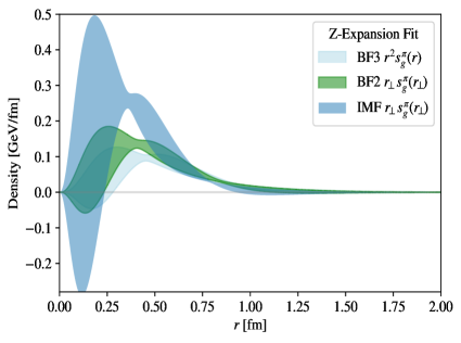
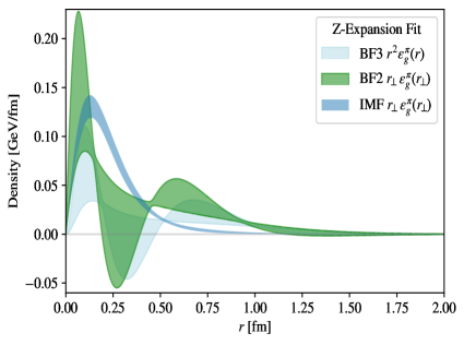
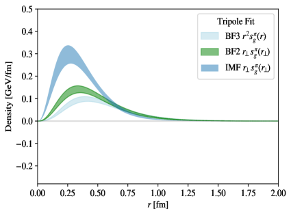
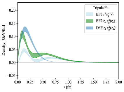
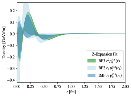
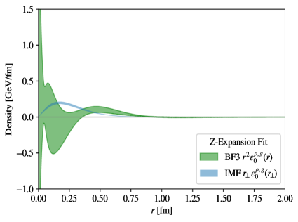
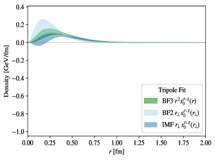
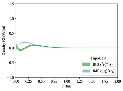
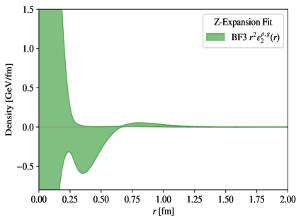
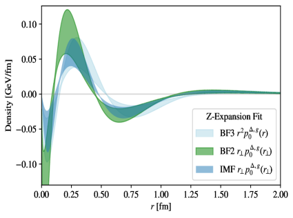
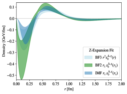
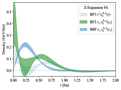
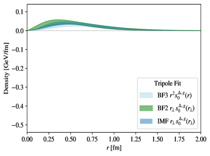
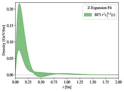
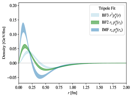
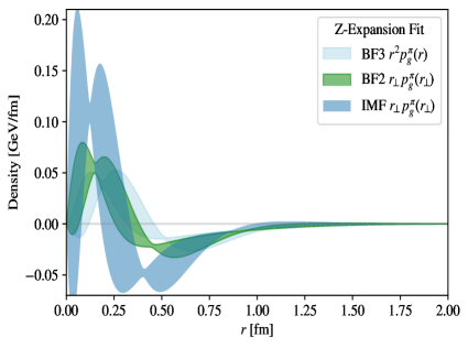
The expressions for the various EMT distributions of the pion in terms of the corresponding GFFs are listed in Appendix B.1. In Fig. 4a, we present our results for the gluon contribution to the energy density ε(r)𝜀𝑟\varepsilon(r), the pressure p(r)𝑝𝑟p(r), and the shear forces s(r)𝑠𝑟s(r) in the 3D and 2D BF, and in the IMF. The definitions of the energy and pressure densities of the individual constituents include the nonconserved GFF c¯(t)¯𝑐𝑡\bar{c}(t), which cancels between the quark and gluon contributions. Since we cannot constrain this term from our calculations, the results shown in Fig. 4a, and for the rest of the hadrons in the sections below, include only the traceless gluon contribution to the densities.
Refer to caption
(a)
Refer to caption
(b)
Refer to caption
(d)
Refer to caption
(f)
Figure 5: Traceless gluon contributions to the pressure (a-b), shear force (c-d), and energy (e-f) distributions of the pion in the 3D BF, 2D BF, and in the IMF. The figures in the left (right) column correspond to densities computed from the tripole (modified z-expansion) fits, with fit parameters given in Table II.1.


Refer to caption
(c)
Refer to caption
(e)

From the pressure density, it is interesting to test whether the 3D and 2D von Laue stability conditions [102] for the total pressure of a composite particle

0𝑑rr2pBF3(r)=0,0𝑑rrpBF2/IMF(r)=0formulae-sequencesuperscriptsubscript0differential-d𝑟superscript𝑟2subscript𝑝BF3𝑟0superscriptsubscript0differential-dsubscript𝑟bottomsubscript𝑟bottomsubscript𝑝BF2/IMFsubscript𝑟bottom0\int_{0}^{\infty}dr~{}r^{2}~{}p_{\text{BF3}}(r)=0,\quad\int_{0}^{\infty}dr_{{\!\bot\!}}~{}r_{{\!\bot\!}}~{}p_{\text{BF2/IMF}}(r_{{\!\bot\!}})=0 (15)

hold for the traceless gluon piece alone. Indeed, by numerical integration we find that the pressures are consistent with the von Laue condition in all frames and using both multipole and z-expansion functional forms to model the t𝑡t dependence of the GFFs. Another important stability condition first shown in Ref. [88] and recently extended in Ref. [98] is that for the total D𝐷D-term

D(0)0,𝐷00D(0)\leq 0\;, (16)

which is satisfied by the gluon contribution to the pion D𝐷D-term in Table II.1. We also find that the hadron stability conditions [88, 99]

pBF3(r)+23sBF3(r)>0pBF2/IMF(r)+12sBF2/IMF(r)>0subscript𝑝BF3𝑟23subscript𝑠BF3𝑟0subscript𝑝BF2/IMFsubscript𝑟bottom12subscript𝑠BF2/IMFsubscript𝑟bottom0\begin{split}p_{\text{BF3}}(r)+\frac{2}{3}s_{\text{BF3}}(r)>0\\ p_{\text{BF2/IMF}}(r_{{\!\bot\!}})+\frac{1}{2}s_{\text{BF2/IMF}}(r_{{\!\bot\!}})>0\end{split} (17)

hold for the traceless gluon piece of the pion pressure and shear force, which allows us to define a partial gluon mechanical mean square radius for the pion rπ,g2expectationsubscriptsuperscript𝑟2𝜋𝑔\braket{r^{2}_{\pi,g}} [see Eq. (63)]. Our results for the mechanical radii as well as the mass radii, defined in Appendix B.1 as appropriate averages of the distance from the center of the hadron weighted by the energy density, are presented in Table III.1.

rπ,g2expectationsubscriptsuperscript𝑟2𝜋𝑔\sqrt{\braket{r^{2}_{\pi,g}}} [fm] BF3 BF2        IMF
Mech. tripole 0.465(19)0..465190.465(19) 0.380(16)0..380160.380(16) 0.294(16)0..294160.294(16)
Mech. z-expansion 0.42(36)0..42360.42(36) 0.34(29)0..34290.34(29) 0.305(30)0..305300.305(30)
Mass tripole 0.435(25)0..435250.435(25) 0.355(20)0..355200.355(20) 0.1594(74)0..1594740.1594(74)
Mass z-expansion 0.452(68)0..452680.452(68) 0.369(56)0..369560.369(56) 0.215(17)0..215170.215(17)
rN,g2expectationsubscriptsuperscript𝑟2𝑁𝑔\sqrt{\braket{r^{2}_{N,g}}} [fm]
Mech. tripole 0.631(68)0..631680.631(68) 0.517(57)0..517570.517(57) 0.517(57)0..517570.517(57)
Mass tripole 0.382(33)0..382330.382(33) 0.312(27)0..312270.312(27) 0.213(14)0..213140.213(14)
Mass z-expansion 0.27(11)0..27110.27(11) 0.217(91)0..217910.217(91) 0.238(38)0..238380.238(38)
rρ,g2expectationsubscriptsuperscript𝑟2𝜌𝑔\sqrt{\braket{r^{2}_{\rho,g}}} [fm]
Mech. tripole 0.278(54)0..278540.278(54) 0.227(35)0..227350.227(35)
Mass tripole 0.371(19)0..371190.371(19) 0.285(15)0..285150.285(15) 0.216(10)0..216100.216(10)
Mass z-expansion 0.329(37)0..329370.329(37) 0.248(32)0..248320.248(32) 0.215(10)0..215100.215(10)
rΔ,g2expectationsubscriptsuperscript𝑟2Δ𝑔\sqrt{\braket{r^{2}_{\Delta,g}}} [fm]
Mech. tripole 0.588(96)0..588960.588(96) 0.471(81)0..471810.471(81) 0.503(77)0..503770.503(77)
Mass tripole 0.387(33)0..387330.387(33) 0.289(28)0..289280.289(28) 0.239(16)0..239160.239(16)
Mass z-expansion 0.20(15)0..20150.20(15) 0.16(23)0..16230.16(23) 0.235(12)0..235120.235(12)
Table 10: Conserved gluon contributions to the mechanical and mass radii of the four hadrons, as defined in Eq. (63) and Appendix B. For the ΔΔ\Delta and ρ𝜌\rho, the contributions from GFFs that were not fit in Sec. II are neglected. Only the mechanical radii corresponding to frames and models for which the mechanical stability requirement of Eq. 17 is satisfied are shown.

III.2 Nucleon

Refer to caption
(a)
Refer to caption
(b)
Refer to caption
(d)
Refer to caption
(f)
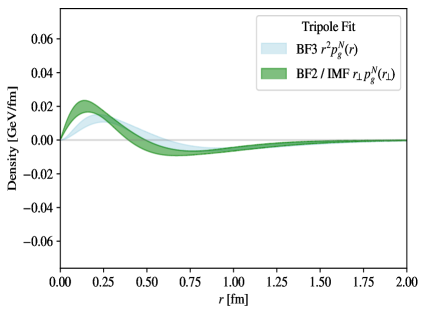
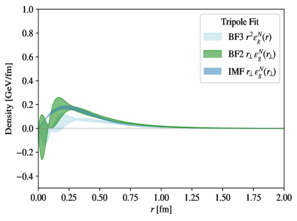
Figure 6: Traceless gluon contributions to the pressure (a-b), shear force (c-d), and energy (e-f) distributions of the nucleon in the 3D BF, 2D BF, and in the IMF. The figures in the left (right) column correspond to the tripole (z-expansion) fits, with fit parameters in Table II.2. The expressions for the pressure and shear force are identical in the 2D BF and the IMF.


Refer to caption
(c)
Refer to caption
(e)

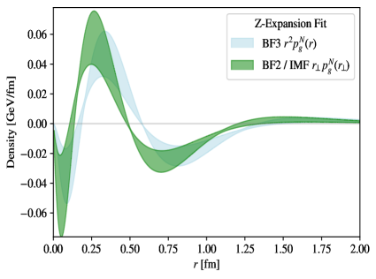
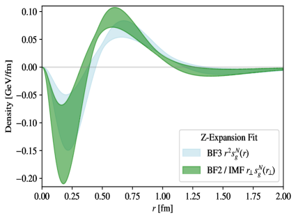
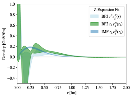
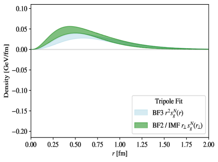
The BF and IMF densities of the nucleon EMT have been studied previously [95, 77, 19, 88] and are defined in Appendix B.2. We note that the 2D Breit frame pressure and shear force coincide with their IMF equivalents. Our results for the symmetric traceless gluon contributions to the densities are shown in Fig. 5a. The difference between the results based on tripole and z-expansion fits to the GFFs is due to the difference between the two fits of DgN(t)superscriptsubscript𝐷𝑔𝑁𝑡D_{g}^{N}(t) in the low t𝑡-t region, as discussed in Sec. II.2. A nonmonotonic gluon DgN(t)superscriptsubscript𝐷𝑔𝑁𝑡D_{g}^{N}(t) causes the traceless gluon pressure to have two nodes, which is different than the form of the quark pressure distribution as found in Ref. [19]. Future lattice, experimental, and phenomenological extractions of DgN(t)subscriptsuperscript𝐷𝑁𝑔𝑡D^{N}_{g}(t) and DqN(t)subscriptsuperscript𝐷𝑁𝑞𝑡D^{N}_{q}(t) will help to clarify the picture.

From the nucleon density results, we find that the pressures in all frames and models are consistent with the von Laue condition (15); however, Eq. (17) is only satisfied for the tripole fit. Moreover, the D𝐷D-term fit by the z-expansion is not strictly positive within uncertainty, and thus we only present the mechanical radius of Eq. (63) for the tripole fit. The mass radii definitions are shown in Appendix B.2, and the corresponding numerical results of all radii are presented in Table III.1.

III.3 ρ𝜌\rho Meson

Beyond the lowest-order energy, pressure, and shear force densities of the pion and the nucleon, the structure of hadrons of spin =1absent1=1 or higher depends on additional quadrupole densities. The BF3 densities and mass radii of the ρ𝜌\rho meson were derived in Refs. [91, 48] and are listed in Appendix B.3. We also derive expressions for the lowest-order BF2 and IMF distributions.

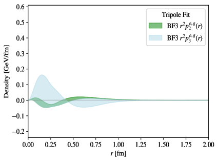
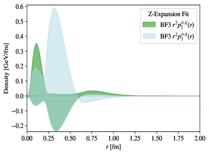
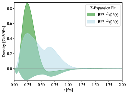
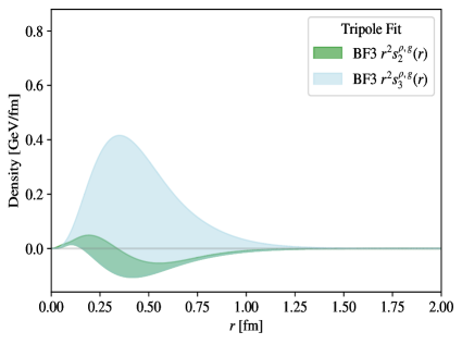
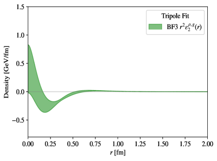
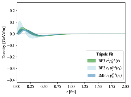
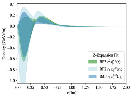
Our numerical results for the lowest-order (Fig. 6a) and higher-order densities (Fig. 7a) are partial and exclude terms depending on D1ρ,g(t)superscriptsubscript𝐷1𝜌𝑔𝑡D_{1}^{\rho,g}(t), since its signal is not well modeled by the ansätze considered here, as discussed in Sec. II.3. We note that almost all of the quadrupole densities are poorly constrained, and therefore we only consider the mechanical stability conditions for the lowest-order densities. In particular, Eq. (17) only holds for the BF3 and BF2 from the tripole GFFs fits. The corresponding mechanical radii of Eq. (63) and the mass radii are shown in Table III.1.
Refer to caption
(a)
Refer to caption
(b)
Refer to caption
(d)
Refer to caption
(f)
Figure 7: Traceless (partial) gluon contributions to the lowest-order pressure (a-b), shear force (c-d), and energy (e-f) distributions of the ρ𝜌\rho meson in the 3D BF, 2D BF, and in the IMF. The figures in the left (right) column correspond to the tripole (z-expansion) fits, with fit parameters in Table II.3. The BF2 contribution to the energy density is not constrained within the range of the figure axes.


Refer to caption
(c)
Refer to caption
(e)
Refer to caption
(a)
Refer to caption
(b)
Refer to caption
(d)
Refer to caption
(f)
Figure 8: Traceless (partial) gluon contributions to the quadrupole order pressure (top), shear force (middle), and energy (bottom) distributions of the ρ𝜌\rho meson in the 3D BF. The figures in the left (right) column correspond to the tripole (z-expansion) fits, with fit parameters in Table II.3.


Refer to caption
(c)
Refer to caption
(e)
Refer to caption
(a)
Refer to caption
(b)
Refer to caption
(d)
Refer to caption
(f)
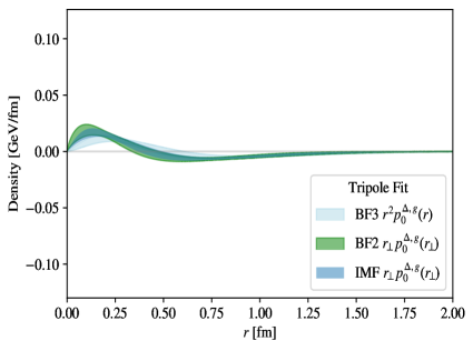
Figure 9: Traceless (partial) gluon contributions to the lowest-order pressure (a-b), shear force (c-d), and energy (e-f) distributions of the ΔΔ\Delta baryon in the 3D BF, 2D BF, and in the IMF. The figures in the left (right) column correspond to the tripole (z-expansion) fits, with fit parameters in Table II.4.


Refer to caption
(c)
Refer to caption
(e)
Refer to caption
(a)
Refer to caption
(b)
Refer to caption
(d)
Refer to caption
(f)
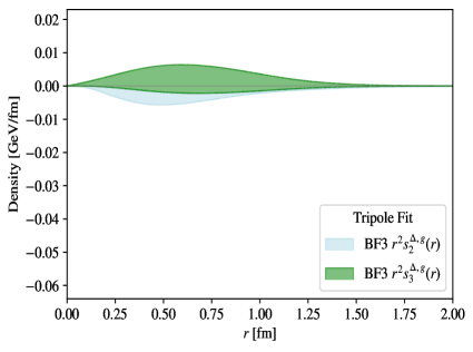
Figure 10: Traceless (partial) gluon contributions to the quadrupole order pressure (a-b), shear force (c-d), and energy (e-f) distributions of the ΔΔ\Delta baryon in the 3D BF. The figures in the left (right) column correspond to the tripole (z-expansion) fits, with fit parameters in Table II.4.


Refer to caption
(c)
Refer to caption
(e)

III.4 ΔΔ\Delta Baryon

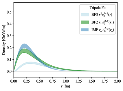
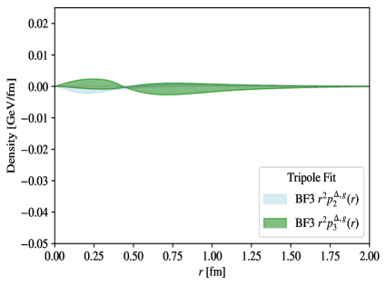
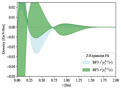
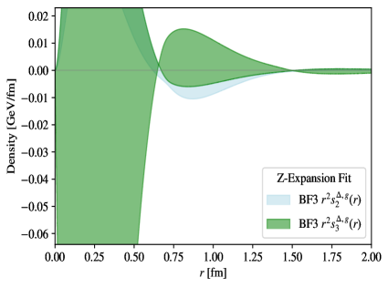
The BF3 distributions for the ΔΔ\Delta baryon were first presented in Ref. [103] and extended in Ref. [36], and are listed in Appendix B.4, along with our derived lowest-order BF2 and IMF contributions to the densities. The higher-order densities are not well constrained, and we limit our mechanical stability check to the lowest-order densities only. We find that Eq. (17) only holds for the tripole fits to the GFFs. Our estimates for the accessible gluon mechanical and mass radii are shown in Table III.1. As discussed in Sec. II.4, we were able to model only four of the ΔΔ\Delta gluon GFFs with the tripole and z-expansion fits, and therefore our results for the gluon densities shown in Figs. 8a and 9a and the radii in Table III.1 are partial.
IV SUMMARY AND CONCLUSION

In this work, we present a lattice QCD extraction of the gluon GFFs of the pion, nucleon, ρ𝜌\rho meson, and ΔΔ\Delta baryon at quark masses corresponding to a pion mass mπ=450(5)MeVsubscript𝑚𝜋4505MeVm_{\pi}=450(5)~{}\text{MeV} in the range 0t<2GeV20𝑡2superscriptGeV20\leq-t<2\;\text{GeV}^{2}. All of the pion and nucleon GFFs, along with six of seven of the ρ𝜌\rho and four of eight of the ΔΔ\Delta GFFs, are fit using the multipole and modified z-expansion models of Eqs. (2) and (3). Most of the GFF fits are consistent between the two models considered, with the most significant exception being the nucleon DgN(t)superscriptsubscript𝐷𝑔𝑁𝑡D_{g}^{N}(t) which, while consistent within error, shows a qualitative difference in behavior between the (monotonic) tripole fit and (nonmonotonic) z-expansion fit. Further calculations with different ensembles are needed in order to determine whether this nonmonotonicity is physical, or the result of poorly quantified systematic uncertainties or a statistical fluctuation in the data. This inconsistency, however, brings to attention the importance of considering a variety of models when studying the GFFs of hadrons at different values of the energy transfer.

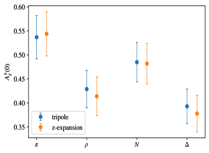
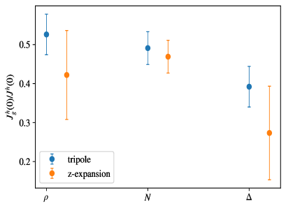
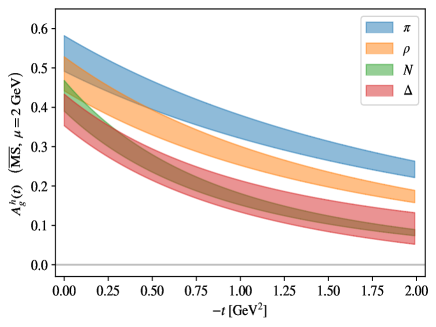
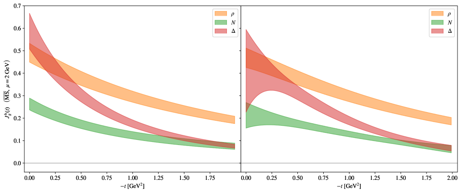
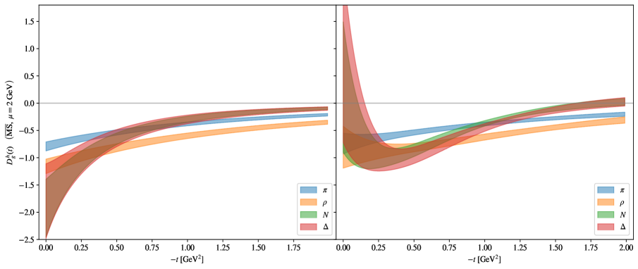
In Figs. 12, 13, and 14 we provide a summary of the gluon contributions to the momentum fraction form factor Ah(t)superscript𝐴𝑡A^{h}(t), angular momentum form factor Jh(t)superscript𝐽𝑡J^{h}(t), and the Dh(t)superscript𝐷𝑡D^{h}(t) form factor. In all cases, the meson GFFs fall off more slowly as functions of t𝑡-t than the baryon GFFs. It will be important for future work to study them at higher magnitudes of energy transfer in order to fully quantify their behavior. In Fig. 11, we summarize the forward limit results for the gluon momentum and spin fractions, with the gluon spin fraction defined as the ratio Jgh(0)/Jh(0)subscriptsuperscript𝐽𝑔0superscript𝐽0J^{h}_{g}(0)/J^{h}(0) of the gluon contribution to the forward-limit angular momentum Jgh(0)subscriptsuperscript𝐽𝑔0J^{h}_{g}(0) and the total spins Jh(0)superscript𝐽0J^{h}(0) of the corresponding hadrons. The gluon momentum fraction is larger for the mesons and smaller for the baryons, decreasing with increasing hadron mass.

Refer to caption
(a)
Refer to caption
(b)
Figure 11: Results for the gluon momentum (a) and spin (b) fractions of the pion, ρ𝜌\rho meson, nucleon, and ΔΔ\Delta baryon as listed in Tables II.1, II.2, II.3, and II.4
Refer to caption
Figure 12: Tripole fits to the Agh(t)superscriptsubscript𝐴𝑔𝑡A_{g}^{h}(t) form factor, corresponding in the forward limit to the gluon contribution to the momentum fraction, for the four hadrons, with fit parameters shown in Tables II.1, II.2, II.3, and II.4. The equivalent figure showing z-expansion fits is indistinguishable.
Refer to caption
Figure 13: Tripole (z-expansion) fits in the left (right) panel to the Jgh(t)superscriptsubscript𝐽𝑔𝑡J_{g}^{h}(t) form factor, corresponding in the forward limit to the gluon contribution to the angular momentum, for the three hadrons, with fit parameters shown in Tables II.2, II.3, and II.4.
Refer to caption
Figure 14: Tripole (z-expansion) fits in the left (right) panel to the Dgh(t)superscriptsubscript𝐷𝑔𝑡D_{g}^{h}(t) form factor for the four hadrons, with fit parameters shown in Tables II.1, II.2, II.3 and II.4.

Additionally, for each model of the t𝑡t dependence of the GFFs we compute the gluon contributions to the hadron energy, pressure, and shear force spatial densities and mass radii, as well as their mechanical radii given stability conditions are satisfied. We consider both the Breit frame and the infinite momentum frame of the densities and the radii. The estimates made using each model are consistent with each other, with the exception of a discrepancy in the nucleon gluon D𝐷D-term and energy, pressure, and shear force densities between the two ansätze, that can be traced to the nonmonotonicity of the DgN(t)superscriptsubscript𝐷𝑔𝑁𝑡D_{g}^{N}(t) z-expansion fit.444The IMF energy density does not depend on DgN(t)superscriptsubscript𝐷𝑔𝑁𝑡D_{g}^{N}(t) and is consistent between the tripole and the modified z-expansion fit.

For the aforementioned hadronic quantities that additionally depend on trace or antisymmetric GFFs, or on the ρ𝜌\rho and ΔΔ\Delta GFFs that are not consistent with our fit models, we provide partial contributions from only the GFFs that we have constrained. In order to better understand in what ways the gluons and quarks separately contribute to the gravitational structure of hadrons, it will be important to constrain all of the GFFs in future studies. Moreover, our renormalization procedure for the gluon EMT does not include mixing with quark operators. Due to the small magnitude of the mixing renormalization coefficient [75, 56], the effect is expected to contribute at the level of a few percent, which is negligible compared to the current statistical uncertainties of the calculation.

This study uses heavier-than-physical quark masses at a single lattice spacing and volume, and therefore our results are subject to unquantified systematic uncertainties that need to be addressed in future studies. For the pion and nucleon, repeating the calculation of the gluon GFFs using different ensembles is critical in order to control the effect of systematic uncertainties for comparisons with future experimental data from J/ψ𝐽𝜓J/\psi and ΥΥ\Upsilon production processes. For unstable hadrons like ρ𝜌\rho and ΔΔ\Delta, lattice QCD methods are the only known way to access their gluon GFFs; studying them at lighter quark masses, where they are not stable, will require more computationally involved Lüscher method analyses [104, 105, 106, 107].

Acknowledgements.
We thank Kyle Cranmer, Will Detmold, Bob Jaffe, William Jay, Andreas Kronfeld, Ethan Neil, and Maxim Polyakov for useful discussions. We also thank Cedric Lorcé for helpful comments on the calculation of densities in different frames, and June-Young Kim and Bao-Dong Sun for sharing their draft manuscript on the structure of spin-3/2 baryons. This work is supported in part by the U.S. Department of Energy, Office of Science, Office of Nuclear Physics, under Grant Contract No. DE-SC0011090. P.E.S. is additionally supported by the National Science Foundation under EAGER Grant No. 2035015, by the U.S. DOE Early Career Award DE-SC0021006, by a NEC research award, and by the Carl G and Shirley Sontheimer Research Fund. This research used resources of the National Energy Research Scientific Computing Center (NERSC), a U.S. Department of Energy Office of Science User Facility operated under Contract No. DE-AC02-05CH11231, as well as resources of the Argonne Leadership Computing Facility, which is a DOE Office of Science User Facility supported under Contract No. DE-AC02-06CH11357, and the Extreme Science and Engineering Discovery Environment (XSEDE), which is supported by National Science Foundation Grant No. ACI-1548562. Computations were carried out in part on facilities of the USQCD Collaboration, which are funded by the Office of Science of the U.S. Department of Energy. The authors thank Robert Edwards, Balint Joo, Kostas Orginos, and the NPLQCD Collaboration for generating the ensembles used in this study. The Chroma [108], QLua [109], QUDA [110, 111, 112], QDP-JIT [113], and QPhiX [114] software libraries were used in this work. Data analysis used NumPy [115], SciPy [116], pandas [117, 118], lsqfit [119], and gvar [120]. Figures were produced using matplotlib [121], seaborn [122], and Mathematica [123].
\do@columngrid

oneΔ

Appendix A NUMERICAL AND ANALYSIS DETAILS

A.1 Symmetric traceless gluon EMT and renormalization

The symmetric traceless part of the EMT, T^μνsuperscript^𝑇𝜇𝜈\hat{T}^{\mu\nu}, can be obtained via the Belinfante-Rosenfeld process555See e.g., the Appendix E of Ref. [124] for a review. [125] and can be decomposed into gluon and quark terms, T^μν=T^gμν+qT^qμνsuperscript^𝑇𝜇𝜈superscriptsubscript^𝑇𝑔𝜇𝜈subscript𝑞superscriptsubscript^𝑇𝑞𝜇𝜈\hat{T}^{\mu\nu}=\hat{T}_{g}^{\mu\nu}+\sum_{q}\hat{T}_{q}^{\mu\nu}, where

T^gμν=2tr[FμαFα+ν14gμνFαβFαβ]T^qμν=iψ¯q𝒟{μγν}ψqigμνψ¯q𝒟ψq,\displaystyle\begin{split}\;\hat{T}_{g}^{\mu\nu}&=2\;\mathrm{tr}\left[F^{\mu\alpha}F_{\alpha}{}^{\nu}+\frac{1}{4}g^{\mu\nu}F^{\alpha\beta}F_{\alpha\beta}\right]\\ \hat{T}_{q}^{\mu\nu}&=i\bar{\psi}_{q}\overleftrightarrow{\mathcal{D}}^{\{\mu}\gamma^{\nu\}}\psi_{q}-ig^{\mu\nu}\bar{\psi}_{q}\overleftrightarrow{\cancel{\mathcal{D}}}\psi_{q}\;,\end{split} (18)

where Fμνsuperscript𝐹𝜇𝜈F^{\mu\nu} is the gluon field-strength tensor of QCD, 𝒟μsubscript𝒟𝜇\mathcal{D}_{\mu} is the covariant derivative, 𝒟μ=(𝒟μ𝒟μ)/2superscript𝒟𝜇superscript𝒟𝜇superscript𝒟𝜇2\overleftrightarrow{\mathcal{D}}^{\mu}=(\overrightarrow{\mathcal{D}}^{\mu}-\overleftarrow{\mathcal{D}}^{\mu})/2, γμsuperscript𝛾𝜇\gamma^{\mu} are the Dirac matrices, the repeated indices are contracted with the Minkowski space-time metric gμνsuperscript𝑔𝜇𝜈g^{\mu\nu}, and the trace is over the color indices.

The gluon field-strength tensor Fμνsuperscript𝐹𝜇𝜈F^{\mu\nu} can be defined up to finite lattice spacing corrections on a Euclidean spacetime lattice as

FμνE(x)=i8g0(Pμν(x)Pμν(x)),superscriptsubscript𝐹𝜇𝜈𝐸𝑥𝑖8subscript𝑔0subscript𝑃𝜇𝜈𝑥subscriptsuperscript𝑃𝜇𝜈𝑥F_{\mu\nu}^{E}(x)=\frac{i}{8g_{0}}(P_{\mu\nu}(x)-P^{\dagger}_{\mu\nu}(x)), (19)

where g0subscript𝑔0g_{0} is the bare gauge coupling, the label E𝐸E denotes Euclidean spacetime, and Pμν(x)subscript𝑃𝜇𝜈𝑥P_{\mu\nu}(x) is the clover term defined in terms of gauge links Uμ(x)subscript𝑈𝜇𝑥U_{\mu}(x) as

Pμν(x)=Uμ(x)Uν(x+μ^)Uμ(x+ν^)Uν(x)+Uν(x)Uμ(xμ^ν^)Uν(xμ^)Uμ(xμ^)+Uμ(xμ^)Uν(xμ^ν^)Uμ(xμ^ν^)Uν(xν^)+Uν(xν^)Uμ(xν^)Uν(xν^+μ^)Uμ(x).subscript𝑃𝜇𝜈𝑥subscript𝑈𝜇𝑥subscript𝑈𝜈𝑥^𝜇subscriptsuperscript𝑈𝜇𝑥^𝜈subscriptsuperscript𝑈𝜈𝑥subscript𝑈𝜈𝑥superscriptsubscript𝑈𝜇𝑥^𝜇^𝜈superscriptsubscript𝑈𝜈𝑥^𝜇subscript𝑈𝜇𝑥^𝜇subscriptsuperscript𝑈𝜇𝑥^𝜇subscriptsuperscript𝑈𝜈𝑥^𝜇^𝜈subscript𝑈𝜇𝑥^𝜇^𝜈subscript𝑈𝜈𝑥^𝜈subscriptsuperscript𝑈𝜈𝑥^𝜈subscript𝑈𝜇𝑥^𝜈subscript𝑈𝜈𝑥^𝜈^𝜇subscriptsuperscript𝑈𝜇𝑥\begin{split}P_{\mu\nu}(x)&=U_{\mu}(x)U_{\nu}(x+\hat{\mu})U^{\dagger}_{\mu}(x+\hat{\nu})U^{\dagger}_{\nu}(x)\\ &+U_{\nu}(x)U_{\mu}^{\dagger}(x-\hat{\mu}-\hat{\nu})U_{\nu}^{\dagger}(x-\hat{\mu})U_{\mu}(x-\hat{\mu})\\ &+U^{\dagger}_{\mu}(x-\hat{\mu})U^{\dagger}_{\nu}(x-\hat{\mu}-\hat{\nu})U_{\mu}(x-\hat{\mu}-\hat{\nu})U_{\nu}(x-\hat{\nu})\\ &+U^{\dagger}_{\nu}(x-\hat{\nu})U_{\mu}(x-\hat{\nu})U_{\nu}(x-\hat{\nu}+\hat{\mu})U^{\dagger}_{\mu}(x)~{}.\end{split} (20)

The momentum-projected traceless symmetric piece of the gluon EMT in Euclidean space can be defined as

T^μνgE(𝚫,τ0)=𝐱ei𝚫𝐱T^μνgE(𝐱,τ0)=𝐱ei𝚫𝐱2tr[FαμE(𝐱,τ0)FανE(𝐱,τ0)14δμνFαβEFαβE],superscriptsubscript^𝑇𝜇𝜈𝑔𝐸𝚫subscript𝜏0subscript𝐱superscript𝑒𝑖𝚫𝐱superscriptsubscript^𝑇𝜇𝜈𝑔𝐸𝐱subscript𝜏0subscript𝐱superscript𝑒𝑖𝚫𝐱2trdelimited-[]superscriptsubscript𝐹𝛼𝜇𝐸𝐱subscript𝜏0superscriptsubscript𝐹𝛼𝜈𝐸𝐱subscript𝜏014subscript𝛿𝜇𝜈subscriptsuperscript𝐹𝐸𝛼𝛽subscriptsuperscript𝐹𝐸𝛼𝛽\hat{T}_{\mu\nu}^{gE}({\mathbf{\Delta}},\tau_{0})=\sum_{{\mathbf{x}}}e^{-i{\mathbf{\Delta}}\cdot{\mathbf{x}}}~{}\hat{T}_{\mu\nu}^{gE}({\mathbf{x}},\tau_{0})=\sum_{{\mathbf{x}}}e^{-i{\mathbf{\Delta}}\cdot{\mathbf{x}}}2\;\mathrm{tr}\left[F_{\alpha\mu}^{E}({\mathbf{x}},\tau_{0})F_{\alpha\nu}^{E}({\mathbf{x}},\tau_{0})-\frac{1}{4}\delta_{\mu\nu}F^{E}_{\alpha\beta}F^{E}_{\alpha\beta}\right]\;, (21)

where the repeated indices are contracted with the Euclidean metric δμνsubscript𝛿𝜇𝜈\delta_{\mu\nu} (i.e. the Kronecker delta in four dimensions) and the trace is over the color indices. In continuous spacetime, a traceless symmetric tensor transforms in the (1,1)11(1,1) representation of the Lorentz group. However, Lorentz symmetry is reduced to hypercubic symmetry on the lattice and therefore lattice operators transform in irreps of the symmetry group H(4)𝐻4H(4). There are two choices of irreps that are safe from power-divergent mixing with lower-dimensional operators, namely τ1(3)superscriptsubscript𝜏13\tau_{1}^{(3)} and τ3(6)superscriptsubscript𝜏36\tau_{3}^{(6)} [126]. We thus project all operator measurements of T^μνgEsubscriptsuperscript^𝑇𝑔𝐸𝜇𝜈\hat{T}^{gE}_{\mu\nu} to particular bases for these two irreps,

T^τ1,1(3)gE=12(T^xxgE+T^yygET^zzgET^ttgE),T^τ1,2(3)gE=12(T^zzgET^ttgE),T^τ1,2(3)gE=12(T^xxgET^yygE),T^τ3,i={1,,6}(6)gE=12(T^μνgE+T^νμgE),μν{xy,xz,xt,yz,yt,zt}.\begin{gathered}\hat{T}^{gE}_{\tau_{1,1}^{(3)}}=\frac{1}{2}(\hat{T}_{xx}^{gE}+\hat{T}_{yy}^{gE}-\hat{T}_{zz}^{gE}-\hat{T}_{tt}^{gE}),\quad\hat{T}^{gE}_{\tau_{1,2}^{(3)}}=\frac{1}{\sqrt{2}}(\hat{T}_{zz}^{gE}-\hat{T}_{tt}^{gE}),\quad\hat{T}^{gE}_{\tau_{1,2}^{(3)}}=\frac{1}{\sqrt{2}}(\hat{T}^{gE}_{xx}-\hat{T}^{gE}_{yy})\;,\\ \hat{T}^{gE}_{\tau_{3,i=\{1,...,6\}}^{(6)}}=\frac{1}{\sqrt{2}}(\hat{T}^{gE}_{\mu\nu}+\hat{T}^{gE}_{\nu\mu}),\quad\mu\nu\in\{xy,xz,xt,yz,yt,zt\}.\end{gathered} (22)

We compute all operators in the τ1(3)superscriptsubscript𝜏13\tau_{1}^{(3)} and τ3(6)superscriptsubscript𝜏36\tau_{3}^{(6)} irreps for all lattice momenta satisfying |𝚫|218(2π/L)2superscript𝚫218superscript2𝜋𝐿2|{\mathbf{\Delta}}|^{2}\leq 18(2\pi/L)^{2}. To suppress gauge noise, we improve the operators by constructing them from gauge links that have been subjected to Wilson flow [127, 128, 129] to flow time t/a2=1𝑡superscript𝑎21t/a^{2}=1 (with integrator step size ϵ=0.01italic-ϵ0.01\epsilon=0.01). Different choices of flow time, as well as use of hypercubic smearing instead of Wilson flow, have been shown to give consistent results [130, 64].

At finite lattice spacing, the two irreps τ1(3)superscriptsubscript𝜏13\tau_{1}^{(3)} and τ3(6)superscriptsubscript𝜏36\tau_{3}^{(6)} renormalize differently and only coincide in the continuum limit, but all operators within each irrep share the same renormalization factor by symmetry. Ref. [60] carried out a nonperturbative RI-MOM calculation [131, 132] of the renormalization factors of these operators on a smaller-volume ensemble for the same parameters as those used in this work. With a one-loop perturbative matching to the MS¯¯MS\overline{\text{MS}} scheme [133], this yielded the renormalization coefficients666Note that these values correspond to 1/g02=β/4Nc1superscriptsubscript𝑔02𝛽4subscript𝑁𝑐1/g_{0}^{2}=\beta/4N_{c} with β=6.1𝛽6.1\beta=6.1, corresponding to the bare lattice operator definition used in this work. For the tadpole-improved Lüscher-Weisz gauge action, this differs from the continuum normalization which is β(12/5u02)/2Nc𝛽125superscriptsubscript𝑢022subscript𝑁𝑐\beta(1-2/5u_{0}^{2})/2N_{c}, where u0subscript𝑢0u_{0} is the tadpole factor. The renormalized operator is independent of this choice.

Zτ1(3)MS¯(μ=2GeV)superscriptsubscript𝑍superscriptsubscript𝜏13¯MS𝜇2GeV\displaystyle Z_{\tau_{1}^{(3)}}^{\overline{\text{MS}}}(\mu=2\;\text{GeV}) =0.9(2)absent0.92\displaystyle=0.9(2) (23)
Zτ3(6)MS¯(μ=2GeV)superscriptsubscript𝑍superscriptsubscript𝜏36¯MS𝜇2GeV\displaystyle Z_{\tau_{3}^{(6)}}^{\overline{\text{MS}}}(\mu=2\;\text{GeV}) =0.78(7)absent0.787\displaystyle=0.78(7)~{}

which renormalize the lattice operators multiplicatively as [T^gE]MS¯=Z[T^gE]lattsuperscriptdelimited-[]superscript^𝑇𝑔𝐸¯MSsubscript𝑍superscriptdelimited-[]superscriptsubscript^𝑇𝑔𝐸latt[\hat{T}^{gE}]^{\overline{\text{MS}}}=Z_{\mathcal{R}}[\hat{T}_{\mathcal{R}}^{gE}]^{\text{latt}} where \mathcal{R} indexes the irrep. The renormalization factors were computed for the same flowed definition as used in this calculation [60]. The uncertainties on these quantities are dominantly systematic and, because they were computed on a different ensemble, uncorrelated with the rest of the data. We choose to model their distribution as uncorrelated Gaussians. As in Ref. [60], we neglect mixing with the quark operators under renormalization, which is expected to contribute at the few-percent level [75, 56].

A.2 Two-point correlation functions

As detailed in the main text, we use a single lattice ensemble in this work; parameters for this ensemble are listed in Table 1. Using matching valence and sea quark actions, we compute two-point functions for varying numbers of light-quark sources on each configuration, using an average of 235 randomly chosen locations (240 for 80% of the configurations, greater-than-or-equivalent-to\gtrsim 200 for 90%). As described below, our analysis accounts for differing numbers of sources by weighting configurations proportionately when drawing bootstrap ensembles. For each source position, we invert from a smeared source (S) and construct propagators for both a point (P) and smeared sink (S), with matching source and sink smearing for the SS propagators, using APE smearing [134] with 35 steps of gauge-invariant Gaussian smearing with width ρ=4.7𝜌4.7\rho=4.7. From each propagator we construct two-point correlation functions for each hadron using the interpolating operators

χπ(x)superscript𝜒𝜋𝑥\displaystyle\chi^{\pi}(x) =ψ¯u(x)γ5ψd(x),absentsubscript¯𝜓𝑢𝑥subscript𝛾5subscript𝜓𝑑𝑥\displaystyle=\overline{\psi}_{u}(x)\gamma_{5}\psi_{d}(x)\;, (24)
χN(x)superscript𝜒𝑁𝑥\displaystyle\chi^{N}(x) =[ψu(x)Cγ5ψd(x)]ψu(x),absentdelimited-[]subscript𝜓𝑢𝑥𝐶subscript𝛾5subscript𝜓𝑑𝑥subscript𝜓𝑢𝑥\displaystyle=\left[\psi_{u}(x)C\gamma_{5}\psi_{d}(x)\right]\psi_{u}(x)\;,
χμρ(x)subscriptsuperscript𝜒𝜌𝜇𝑥\displaystyle\chi^{\rho}_{\mu}(x) =ψ¯u(x)γμψd(x),absentsubscript¯𝜓𝑢𝑥subscript𝛾𝜇subscript𝜓𝑑𝑥\displaystyle=\overline{\psi}_{u}(x)\gamma_{\mu}\psi_{d}(x)\;,
χμΔ(x)subscriptsuperscript𝜒Δ𝜇𝑥\displaystyle\chi^{\Delta}_{\mu}(x) =[ψu(x)Cγμψu(x)]ψu(x),absentdelimited-[]subscript𝜓𝑢𝑥𝐶subscript𝛾𝜇subscript𝜓𝑢𝑥subscript𝜓𝑢𝑥\displaystyle=\left[\psi_{u}(x)C\gamma_{\mu}\psi_{u}(x)\right]\psi_{u}(x)\;,

where all gamma matrices are Euclidean, C𝐶C is the charge conjugation matrix, and color and spinor indices are left implicit.

The interpolating operators overlap with the lowest-lying hadronic states as

0|bra0\displaystyle\bra{0} χπ(x)superscript𝜒𝜋𝑥\displaystyle\chi^{\pi}(x) |π(𝐩)ket𝜋𝐩\displaystyle\ket{\pi({\mathbf{p}})} =Z𝐩πei𝐩𝐱,absentsubscriptsuperscript𝑍𝜋𝐩superscript𝑒𝑖𝐩𝐱\displaystyle=Z^{\pi}_{{\mathbf{p}}}e^{i{\mathbf{p}}\cdot{\mathbf{x}}}\;, (25)
0|bra0\displaystyle\bra{0} χN(x)superscript𝜒𝑁𝑥\displaystyle\chi^{N}(x) |N(𝐩,σ)ket𝑁𝐩𝜎\displaystyle\ket{N({\mathbf{p}},\sigma)} =Z𝐩Nu(𝐩,σ)ei𝐩𝐱,absentsubscriptsuperscript𝑍𝑁𝐩𝑢𝐩𝜎superscript𝑒𝑖𝐩𝐱\displaystyle=Z^{N}_{{\mathbf{p}}}u({\mathbf{p}},\sigma)e^{i{\mathbf{p}}\cdot{\mathbf{x}}}\;,
0|bra0\displaystyle\bra{0} χaρ(x)subscriptsuperscript𝜒𝜌𝑎𝑥\displaystyle\chi^{\rho}_{a}(x) |ρ(𝐩,λ)ket𝜌𝐩𝜆\displaystyle\ket{\rho({\mathbf{p}},\lambda)} =Z𝐩ρϵa(𝐩,λ)ei𝐩𝐱,absentsubscriptsuperscript𝑍𝜌𝐩subscriptitalic-ϵ𝑎𝐩𝜆superscript𝑒𝑖𝐩𝐱\displaystyle=Z^{\rho}_{{\mathbf{p}}}\epsilon_{a}({\mathbf{p}},\lambda)e^{i{\mathbf{p}}\cdot{\mathbf{x}}}\;,
0|bra0\displaystyle\bra{0} χaΔ(x)subscriptsuperscript𝜒Δ𝑎𝑥\displaystyle\chi^{\Delta}_{a}(x) |Δ(𝐩,ξ)ketΔ𝐩𝜉\displaystyle\ket{\Delta({\mathbf{p}},\xi)} =Z𝐩Δua(𝐩,ξ)ei𝐩𝐱,absentsubscriptsuperscript𝑍Δ𝐩subscript𝑢𝑎𝐩𝜉superscript𝑒𝑖𝐩𝐱\displaystyle=Z^{\Delta}_{{\mathbf{p}}}u_{a}({\mathbf{p}},\xi)e^{i{\mathbf{p}}\cdot{\mathbf{x}}}\;,

where Z𝐩subscript𝑍𝐩Z_{{\mathbf{p}}} is an overlap factor, ϵa(𝐩,λ)subscriptitalic-ϵ𝑎𝐩𝜆\epsilon_{a}({\mathbf{p}},\lambda) is a spin-1 polarization vector with λ{1,0,1}𝜆101\lambda\in\{1,0,-1\} and in a spherical basis a{+,,0}𝑎0{a\in\{+,-,0\}} such that

ϵa(𝐩,λ)={12[ϵx(𝐩,λ)±iϵy(𝐩,λ)],a=±ϵz(𝐩,λ),a=0,subscriptitalic-ϵ𝑎𝐩𝜆cases12delimited-[]plus-or-minussubscriptitalic-ϵ𝑥𝐩𝜆𝑖subscriptitalic-ϵ𝑦𝐩𝜆𝑎plus-or-minussubscriptitalic-ϵ𝑧𝐩𝜆𝑎0\epsilon_{a}({\mathbf{p}},\lambda)=\begin{cases}\frac{1}{\sqrt{2}}[\epsilon_{x}({\mathbf{p}},\lambda)\pm i\epsilon_{y}({\mathbf{p}},\lambda)],&a=\pm\\ \epsilon_{z}({\mathbf{p}},\lambda),&a=0\;,\end{cases} (26)

u(𝐩,σ)𝑢𝐩𝜎u({\mathbf{p}},\sigma) with σ{12,12}𝜎1212\sigma\in\{\frac{1}{2},-\frac{1}{2}\} is a Dirac spinor, and ua(𝐩,ξ)subscript𝑢𝑎𝐩𝜉u_{a}({\mathbf{p}},\xi) is a Rarita-Schwinger spin vector with ξ{32,12,12,32}𝜉32121232\xi\in\{\frac{3}{2},\frac{1}{2},-\frac{1}{2},-\frac{3}{2}\}, written in the same spherical basis as ϵa(𝐩,λ)subscriptitalic-ϵ𝑎𝐩𝜆\epsilon_{a}({\mathbf{p}},\lambda) in Eq. (26).

The momentum projected two-point correlation function of the pion can be expressed as

Cπ,2pt(𝐩,t;𝐱0,t0)=𝐱ei𝐩(𝐱𝐱0)χπ(𝐱,t)χπ(𝐱0,t0)teE𝐩πt2E𝐩πZ~𝐩Z𝐩,superscript𝐶𝜋2pt𝐩superscript𝑡subscript𝐱0subscript𝑡0subscript𝐱superscript𝑒𝑖𝐩𝐱subscript𝐱0delimited-⟨⟩superscript𝜒𝜋𝐱superscript𝑡superscript𝜒𝜋subscript𝐱0subscript𝑡0superscript𝑡superscript𝑒subscriptsuperscript𝐸𝜋𝐩superscript𝑡2subscriptsuperscript𝐸𝜋𝐩subscript~𝑍𝐩subscript𝑍𝐩C^{\pi,\text{2pt}}({\mathbf{p}},t^{\prime};{\mathbf{x}}_{0},t_{0})=\sum_{{\mathbf{x}}}e^{-i{\mathbf{p}}\cdot({\mathbf{x}}-{\mathbf{x}}_{0})}\langle\chi^{\pi}({\mathbf{x}},t^{\prime})\chi^{\pi\dagger}({\mathbf{x}}_{0},t_{0})\rangle\xrightarrow{t^{\prime}\rightarrow\infty}\frac{e^{-E^{\pi}_{\mathbf{p}}t^{\prime}}}{2E^{\pi}_{\mathbf{p}}}\tilde{Z}_{{\mathbf{p}}}Z_{{\mathbf{p}}}\;, (27)

where E𝐩πsuperscriptsubscript𝐸𝐩𝜋E_{{\mathbf{p}}}^{\pi} is the energy of the lowest-lying state with momentum 𝐩𝐩{\mathbf{p}}, and Z~𝐩Z𝐩subscript~𝑍𝐩subscript𝑍𝐩\tilde{Z}_{{\mathbf{p}}}\neq Z_{{\mathbf{p}}} when the source and sink are smeared differently. The two-point correlation function of the nucleon for spin channel σσ𝜎superscript𝜎\sigma\rightarrow\sigma^{\prime} is

CσσN,2pt(𝐩,t;𝐱0,t0)=𝐱ei𝐩(𝐱𝐱0)tr[ΓσσχN(𝐱,t)χ¯N(𝐱0,t0)]teE𝐩Nt2E𝐩NZ~𝐩Z𝐩tr[Γσσ(p+mN)],subscriptsuperscript𝐶𝑁2pt𝜎superscript𝜎𝐩superscript𝑡subscript𝐱0subscript𝑡0subscript𝐱superscript𝑒𝑖𝐩𝐱subscript𝐱0trdelimited-[]subscriptΓsuperscript𝜎𝜎delimited-⟨⟩superscript𝜒𝑁𝐱superscript𝑡superscript¯𝜒𝑁subscript𝐱0subscript𝑡0superscript𝑡superscript𝑒subscriptsuperscript𝐸𝑁𝐩superscript𝑡2subscriptsuperscript𝐸𝑁𝐩subscript~𝑍𝐩subscript𝑍𝐩trdelimited-[]subscriptΓsuperscript𝜎𝜎cancel𝑝subscript𝑚𝑁C^{N,\text{2pt}}_{\sigma\sigma^{\prime}}({\mathbf{p}},t^{\prime};{\mathbf{x}}_{0},t_{0})=\sum_{{\mathbf{x}}}e^{-i{\mathbf{p}}\cdot({\mathbf{x}}-{\mathbf{x}}_{0})}\mathrm{tr}\big{[}\Gamma_{\sigma^{\prime}\sigma}\langle\chi^{N}({\mathbf{x}},t^{\prime})\bar{\chi}^{N}({\mathbf{x}}_{0},t_{0})\rangle\big{]}\xrightarrow{t^{\prime}\rightarrow\infty}\frac{e^{-E^{N}_{\mathbf{p}}t^{\prime}}}{2E^{N}_{\mathbf{p}}}\tilde{Z}_{{\mathbf{p}}}Z_{{\mathbf{p}}}\mathrm{tr}\big{[}\Gamma_{\sigma^{\prime}\sigma}(\cancel{p}+m_{N})\big{]}\;, (28)

where χ¯=χγt¯𝜒superscript𝜒subscript𝛾𝑡\bar{\chi}=\chi^{\dagger}\gamma_{t}, traces are over Dirac indices, and ΓσσsubscriptΓsuperscript𝜎𝜎\Gamma_{\sigma^{\prime}\sigma} is a 2×2222\times 2 block matrix that projects the four different spin channels of the nucleon [135], i.e.

Γσσ=(P+(1+γxγy)P+γz(γx+iγy)P+γz(γxiγy)P+(1γxγy))σσ,subscriptΓsuperscript𝜎𝜎subscriptmatrixsubscript𝑃1subscript𝛾𝑥subscript𝛾𝑦subscript𝑃subscript𝛾𝑧subscript𝛾𝑥𝑖subscript𝛾𝑦subscript𝑃subscript𝛾𝑧subscript𝛾𝑥𝑖subscript𝛾𝑦subscript𝑃1subscript𝛾𝑥subscript𝛾𝑦superscript𝜎𝜎\Gamma_{\sigma^{\prime}\sigma}=\begin{pmatrix}P_{+}(1+\gamma_{x}\gamma_{y})&P_{+}\gamma_{z}(\gamma_{x}+i\gamma_{y})\\ P_{+}\gamma_{z}(\gamma_{x}-i\gamma_{y})&P_{+}(1-\gamma_{x}\gamma_{y})\end{pmatrix}_{\sigma^{\prime}\sigma}\;, (29)

where P+12(1+γt)subscript𝑃121subscript𝛾𝑡P_{+}\equiv\frac{1}{2}(1+\gamma_{t}) is a positive-energy projector. We use all four possible channels σ,σ{+1/2,1/2}𝜎superscript𝜎1212\sigma,\sigma^{\prime}\in\{+1/2,-1/2\}, adding significant additional data over the analysis in Ref. [60] where only the two spin-conserving channels were used. The two-point correlation function of the ρ𝜌\rho meson, in the spherical basis of one of the 9 spin channels aa𝑎superscript𝑎a\rightarrow a^{\prime}, can be expressed as

Caaρ,2pt(𝐩,t;𝐱0,t0)=𝐱ei𝐩(𝐱𝐱0)χaρ(𝐱,t)χaρ(𝐱0,t0)teE𝐩ρt2E𝐩ρZ~𝐩Z𝐩Λaa(ρ)(𝐩),subscriptsuperscript𝐶𝜌2pt𝑎superscript𝑎𝐩superscript𝑡subscript𝐱0subscript𝑡0subscript𝐱superscript𝑒𝑖𝐩𝐱subscript𝐱0delimited-⟨⟩superscriptsubscript𝜒superscript𝑎𝜌𝐱superscript𝑡superscriptsubscript𝜒𝑎𝜌subscript𝐱0subscript𝑡0superscript𝑡superscript𝑒subscriptsuperscript𝐸𝜌𝐩superscript𝑡2subscriptsuperscript𝐸𝜌𝐩subscript~𝑍𝐩subscript𝑍𝐩superscriptsubscriptΛsuperscript𝑎𝑎𝜌𝐩C^{\rho,\text{2pt}}_{aa^{\prime}}({\mathbf{p}},t^{\prime};{\mathbf{x}}_{0},t_{0})=\sum_{{\mathbf{x}}}e^{-i{\mathbf{p}}\cdot({\mathbf{x}}-{\mathbf{x}}_{0})}\langle\chi_{a^{\prime}}^{\rho}({\mathbf{x}},t^{\prime})\chi_{a}^{\rho\dagger}({\mathbf{x}}_{0},t_{0})\rangle\xrightarrow{t^{\prime}\rightarrow\infty}\frac{e^{-E^{\rho}_{\mathbf{p}}t^{\prime}}}{2E^{\rho}_{\mathbf{p}}}\tilde{Z}_{{\mathbf{p}}}Z_{{\mathbf{p}}}\Lambda_{a^{\prime}a}^{(\rho)}({\mathbf{p}})\;, (30)

where Λaa(ρ)(𝐩)λϵa(𝐩,λ)ϵa(𝐩,λ)subscriptsuperscriptΛ𝜌superscript𝑎𝑎𝐩subscript𝜆subscriptitalic-ϵsuperscript𝑎𝐩𝜆subscriptsuperscriptitalic-ϵ𝑎𝐩𝜆\Lambda^{(\rho)}_{a^{\prime}a}({\mathbf{p}})\equiv\sum_{\lambda}\epsilon_{a^{\prime}}({\mathbf{p}},\lambda)\epsilon^{*}_{a}({\mathbf{p}},\lambda) [cf. Eq. (9)]. Finally, we compute the two-point correlator of the ΔΔ\Delta baryon for the 10 spin channels ξξ𝜉superscript𝜉\xi\rightarrow\xi^{\prime} where ξξ𝜉superscript𝜉\xi\geq\xi^{\prime},

CξξΔ,2pt(𝐩,t;𝐱0,t0)=𝐱ei𝐩(𝐱𝐱0)tr[𝒟σ,aξ𝒟σ,aξΓσσχaΔ(𝐱,t)χ¯aΔ(𝐱0,t0)]teE𝐩Δt2E𝐩ΔZ~𝐩Z𝐩tr[𝒟σ,aξ𝒟σ,aξΓσσΛaa(Δ)(𝐩)],subscriptsuperscript𝐶Δ2pt𝜉superscript𝜉𝐩superscript𝑡subscript𝐱0subscript𝑡0subscript𝐱superscript𝑒𝑖𝐩𝐱subscript𝐱0trdelimited-[]subscriptsuperscript𝒟𝜉𝜎𝑎subscriptsuperscript𝒟superscript𝜉superscript𝜎superscript𝑎subscriptΓsuperscript𝜎𝜎delimited-⟨⟩superscriptsubscript𝜒superscript𝑎Δ𝐱superscript𝑡superscriptsubscript¯𝜒𝑎Δsubscript𝐱0subscript𝑡0superscript𝑡superscript𝑒subscriptsuperscript𝐸Δ𝐩superscript𝑡2subscriptsuperscript𝐸Δ𝐩subscript~𝑍𝐩subscript𝑍𝐩trdelimited-[]subscriptsuperscript𝒟𝜉𝜎𝑎subscriptsuperscript𝒟superscript𝜉superscript𝜎superscript𝑎subscriptΓsuperscript𝜎𝜎subscriptsuperscriptΛΔsuperscript𝑎𝑎𝐩\begin{split}C^{\Delta,\text{2pt}}_{\xi\xi^{\prime}}({\mathbf{p}},t^{\prime};{\mathbf{x}}_{0},t_{0})&=\sum_{{\mathbf{x}}}e^{-i{\mathbf{p}}\cdot({\mathbf{x}}-{\mathbf{x}}_{0})}\mathrm{tr}\big{[}\mathcal{D}^{\xi}_{\sigma,a}\mathcal{D}^{\xi^{\prime}}_{\sigma^{\prime},a^{\prime}}\Gamma_{\sigma^{\prime}\sigma}\langle\chi_{a^{\prime}}^{\Delta}({\mathbf{x}},t^{\prime})\bar{\chi}_{a}^{\Delta}({\mathbf{x}}_{0},t_{0})\rangle\big{]}\\ &\xrightarrow{t^{\prime}\rightarrow\infty}\frac{e^{-E^{\Delta}_{\mathbf{p}}t^{\prime}}}{2E^{\Delta}_{\mathbf{p}}}\tilde{Z}_{{\mathbf{p}}}Z_{{\mathbf{p}}}\mathrm{tr}\big{[}\mathcal{D}^{\xi}_{\sigma,a}\mathcal{D}^{\xi^{\prime}}_{\sigma^{\prime},a^{\prime}}\Gamma_{\sigma^{\prime}\sigma}\Lambda^{(\Delta)}_{a^{\prime}a}({\mathbf{p}})\big{]}\;,\end{split} (31)

where repeated indices are summed over, Λaa(Δ)(𝐩)ξua(𝐩,ξ)u¯a(𝐩,ξ)subscriptsuperscriptΛΔsuperscript𝑎𝑎𝐩subscript𝜉subscript𝑢superscript𝑎𝐩𝜉subscript¯𝑢𝑎𝐩𝜉\Lambda^{(\Delta)}_{a^{\prime}a}({\mathbf{p}})\equiv\sum_{\xi}u_{a^{\prime}}({\mathbf{p}},\xi)\bar{u}_{a}({\mathbf{p}},\xi) [cf. Eq. (11)], and the coefficients 𝒟σ,aξsubscriptsuperscript𝒟𝜉𝜎𝑎\mathcal{D}^{\xi}_{\sigma,a} are defined such that

𝒟1/2,+3/2=𝒟1/2,3/2=𝒟1/2,01/2=𝒟1/2,01/2=1,superscriptsubscript𝒟1232superscriptsubscript𝒟1232superscriptsubscript𝒟12012superscriptsubscript𝒟120121\mathcal{D}_{1/2,+}^{3/2}=\mathcal{D}_{-1/2,-}^{-3/2}=\mathcal{D}_{1/2,0}^{1/2}=\mathcal{D}_{-1/2,0}^{-1/2}=1\;, (32)

and 𝒟σ,aξ=0subscriptsuperscript𝒟𝜉𝜎𝑎0\mathcal{D}^{\xi}_{\sigma,a}=0 for all other choices of {ξ,σ,a}𝜉𝜎𝑎\{\xi,\sigma,a\}.777For the +3/21/23212+3/2\rightarrow-1/2 channel we instead computed correlation functions corresponding to 𝒟1/2,+3/2=𝒟1/2,1/2=1subscriptsuperscript𝒟3212subscriptsuperscript𝒟12121\mathcal{D}^{3/2}_{1/2,+}=\mathcal{D}^{-1/2}_{1/2,-}=1.

We average over sources to obtain per-configuration measurements Cssh,2pt(𝐩,tf=tt0)superscriptsubscript𝐶𝑠superscript𝑠2pt𝐩subscript𝑡𝑓superscript𝑡subscript𝑡0C_{ss^{\prime}}^{h,\text{2pt}}({\bf p},t_{f}=t^{\prime}-t_{0}) for each hadron hh, weighting this average by the number of sources on each configuration when forming bootstrap ensembles as discussed below. The effective mass for each hadron hh is defined as

mheff(tf)=log(sCssh,2pt(𝟎,tf)sCssh,2pt(𝟎,tf+1))subscriptsuperscript𝑚effsubscript𝑡𝑓subscript𝑠subscriptsuperscript𝐶2pt𝑠𝑠0subscript𝑡𝑓subscript𝑠subscriptsuperscript𝐶2pt𝑠𝑠0subscript𝑡𝑓1m^{\text{eff}}_{h}(t_{f})=\log\left(\frac{\sum_{s}C^{h,\text{2pt}}_{ss}({\mathbf{0}},t_{f})}{\sum_{s}C^{h,\text{2pt}}_{ss}({\mathbf{0}},t_{f}+1)}\right) (33)

and constructed from the spin-averaged (over diagonal spin channels for states with spin 0absent0\neq 0) two-point functions. The results for each hadron are shown in Fig. 15, along with the numerical values that we use for the hadron masses mhsubscript𝑚m_{h} throughout this work, which are obtained via single-state correlated fits to Eq. (33), in regions in which the excited-state contamination is smaller than the statistical uncertainties of the effective mass function. The numerical values are given in Table 11.

Refer to caption
Figure 15: Effective mass functions for all four hadrons, with the results obtained using the SP (SS) correlation functions shown in solid (translucent) color. The dashed line indicates the numerical values used to compute kinematic coefficients, as listed in Table 11.

A.3 Three-point correlation functions and ratios

We construct hadronic three-point functions of the gluon EMT operator, which are defined as

C,iπ,3pt(𝐩,𝐩;t,τ;𝐱𝟎,t0)superscriptsubscript𝐶𝑖𝜋3pt𝐩superscript𝐩superscript𝑡𝜏subscript𝐱0subscript𝑡0\displaystyle C_{\mathcal{R},i}^{\pi,\text{3pt}}({\mathbf{p}},{\mathbf{p}}^{\prime};t^{\prime},\tau;{\mathbf{x_{0}}},t_{0}) =𝐱,𝐲ei𝐩(𝐱𝐱0)ei𝚫(𝐲𝐱0)χπ(𝐱,t)T^,igE(𝐲,τ+t0)χπ(𝐱𝟎,t0)absentsubscript𝐱𝐲superscript𝑒𝑖superscript𝐩𝐱subscript𝐱0superscript𝑒𝑖𝚫𝐲subscript𝐱0delimited-⟨⟩superscript𝜒𝜋𝐱superscript𝑡subscriptsuperscript^𝑇𝑔𝐸𝑖𝐲𝜏subscript𝑡0superscript𝜒𝜋subscript𝐱0subscript𝑡0\displaystyle=\sum_{{\mathbf{x}},{\mathbf{y}}}e^{-i{\mathbf{p}}^{\prime}\cdot({\mathbf{x}}-{\mathbf{x}}_{0})}e^{i{\mathbf{\Delta}}\cdot({\mathbf{y}}-{\mathbf{x}}_{0})}\langle\chi^{\pi}({\mathbf{x}},t^{\prime})\hat{T}^{gE}_{\mathcal{R},i}({\mathbf{y}},\tau+t_{0})\chi^{\pi\dagger}({\mathbf{x_{0}}},t_{0})\rangle (34)
Cσσ;,iN,3pt(𝐩,𝐩;t,τ;𝐱𝟎,t0)superscriptsubscript𝐶𝜎superscript𝜎𝑖𝑁3pt𝐩superscript𝐩superscript𝑡𝜏subscript𝐱0subscript𝑡0\displaystyle C_{\sigma\sigma^{\prime};\mathcal{R},i}^{N,\text{3pt}}({\mathbf{p}},{\mathbf{p}}^{\prime};t^{\prime},\tau;{\mathbf{x_{0}}},t_{0}) =𝐱,𝐲ei𝐩(𝐱𝐱0)ei𝚫(𝐲𝐱0)tr[ΓσσNχN(𝐱,t)T^,igE(𝐲,τ+t0)χ¯N(𝐱𝟎,t0)]absentsubscript𝐱𝐲superscript𝑒𝑖superscript𝐩𝐱subscript𝐱0superscript𝑒𝑖𝚫𝐲subscript𝐱0trdelimited-[]subscriptsuperscriptΓ𝑁superscript𝜎𝜎delimited-⟨⟩superscript𝜒𝑁𝐱superscript𝑡subscriptsuperscript^𝑇𝑔𝐸𝑖𝐲𝜏subscript𝑡0superscript¯𝜒𝑁subscript𝐱0subscript𝑡0\displaystyle=\sum_{{\mathbf{x}},{\mathbf{y}}}e^{-i{\mathbf{p}}^{\prime}\cdot({\mathbf{x}}-{\mathbf{x}}_{0})}e^{i{\mathbf{\Delta}}\cdot({\mathbf{y}}-{\mathbf{x}}_{0})}\text{tr}[\Gamma^{N}_{\sigma^{\prime}\sigma}\langle\chi^{N}({\mathbf{x}},t^{\prime})\hat{T}^{gE}_{\mathcal{R},i}({\mathbf{y}},\tau+t_{0})~{}\bar{\chi}^{N}({\mathbf{x_{0}}},t_{0})\rangle] (35)
Caa;,iρ,3pt(𝐩,𝐩;t,τ;𝐱𝟎,t0)superscriptsubscript𝐶𝑎superscript𝑎𝑖𝜌3pt𝐩superscript𝐩superscript𝑡𝜏subscript𝐱0subscript𝑡0\displaystyle C_{aa^{\prime};\mathcal{R},i}^{\rho,\text{3pt}}({\mathbf{p}},{\mathbf{p}}^{\prime};t^{\prime},\tau;{\mathbf{x_{0}}},t_{0}) =𝐱,𝐲ei𝐩(𝐱𝐱0)ei𝚫(𝐲𝐱0)χaρ(𝐱,t)T^,igE(𝐲,τ+t0)χaρ(𝐱𝟎,t0)absentsubscript𝐱𝐲superscript𝑒𝑖superscript𝐩𝐱subscript𝐱0superscript𝑒𝑖𝚫𝐲subscript𝐱0delimited-⟨⟩superscriptsubscript𝜒superscript𝑎𝜌𝐱superscript𝑡subscriptsuperscript^𝑇𝑔𝐸𝑖𝐲𝜏subscript𝑡0superscriptsubscript𝜒𝑎𝜌subscript𝐱0subscript𝑡0\displaystyle=\sum_{{\mathbf{x}},{\mathbf{y}}}e^{-i{\mathbf{p}}^{\prime}\cdot({\mathbf{x}}-{\mathbf{x}}_{0})}e^{i{\mathbf{\Delta}}\cdot({\mathbf{y}}-{\mathbf{x}}_{0})}~{}\langle\chi_{a^{\prime}}^{\rho}({\mathbf{x}},t^{\prime})\hat{T}^{gE}_{\mathcal{R},i}({\mathbf{y}},\tau+t_{0})\chi_{a}^{\rho\dagger}({\mathbf{x_{0}}},t_{0})\rangle (36)
Cξξ;,iΔ,3pt(𝐩,𝐩;t,τ;𝐱𝟎,t0)superscriptsubscript𝐶𝜉superscript𝜉𝑖Δ3pt𝐩superscript𝐩superscript𝑡𝜏subscript𝐱0subscript𝑡0\displaystyle C_{\xi\xi^{\prime};\mathcal{R},i}^{\Delta,\text{3pt}}({\mathbf{p}},{\mathbf{p}}^{\prime};t^{\prime},\tau;{\mathbf{x_{0}}},t_{0}) =𝐱,𝐲ei𝐩(𝐱𝐱0)ei𝚫(𝐲𝐱0)tr[𝒟σ,aξ𝒟σ,aξΓσσΔχaΔ(𝐱,t)T^,igE(𝐲,τ+t0)χ¯aΔ(𝐱𝟎,t0)]absentsubscript𝐱𝐲superscript𝑒𝑖superscript𝐩𝐱subscript𝐱0superscript𝑒𝑖𝚫𝐲subscript𝐱0trdelimited-[]subscriptsuperscript𝒟𝜉𝜎𝑎subscriptsuperscript𝒟superscript𝜉superscript𝜎superscript𝑎superscriptsubscriptΓsuperscript𝜎𝜎Δdelimited-⟨⟩superscriptsubscript𝜒superscript𝑎Δ𝐱superscript𝑡subscriptsuperscript^𝑇𝑔𝐸𝑖𝐲𝜏subscript𝑡0superscriptsubscript¯𝜒𝑎Δsubscript𝐱0subscript𝑡0\displaystyle=\sum_{{\mathbf{x}},{\mathbf{y}}}e^{-i{\mathbf{p}}^{\prime}\cdot({\mathbf{x}}-{\mathbf{x}}_{0})}e^{i{\mathbf{\Delta}}\cdot({\mathbf{y}}-{\mathbf{x}}_{0})}~{}\text{tr}[\mathcal{D}^{\xi}_{\sigma,a}\mathcal{D}^{\xi^{\prime}}_{\sigma^{\prime},a^{\prime}}\Gamma_{\sigma^{\prime}\sigma}^{\Delta}\langle\chi_{a^{\prime}}^{\Delta}({\mathbf{x}},t^{\prime})\hat{T}^{gE}_{\mathcal{R},i}({\mathbf{y}},\tau+t_{0})\bar{\chi}_{a}^{\Delta}({\mathbf{x_{0}}},t_{0})\rangle] (37)

where repeated indices are summed over, (𝐱0,t0)subscript𝐱0subscript𝑡0({\mathbf{x}}_{0},t_{0}) and (𝐱,t)𝐱superscript𝑡({\mathbf{x}},t^{\prime}) are the source and sink positions, (𝐲,τ)𝐲𝜏({\mathbf{y}},\tau) is the operator insertion position, 𝐩𝐩{\mathbf{p}} and 𝐩superscript𝐩{\mathbf{p}}^{\prime} are the three-momenta of the hadron at the source and sink, 𝚫=𝐩𝐩𝚫superscript𝐩𝐩{\mathbf{\Delta}}={\mathbf{p}}^{\prime}-{\mathbf{p}} is the three-momentum injected by the operator, and T^,igEsubscriptsuperscript^𝑇𝑔𝐸𝑖\hat{T}^{gE}_{\mathcal{R},i} is a gluon EMT operator projected to irrep \mathcal{R} and basis element i𝑖i as defined in Eq. (22). These three-point functions are entirely disconnected and so may be computed by correlating two-point functions with measurements of the gluon EMT, i.e. by computing

Css;,ih,3pt(𝐩,𝐩;t,τ;𝐱𝟎,t0)=ei𝚫𝐱0Cssh,2pt(𝐩,t;𝐱𝟎,t0)T^,igE(𝚫,τ+t0),superscriptsubscript𝐶𝑠superscript𝑠𝑖3pt𝐩superscript𝐩superscript𝑡𝜏subscript𝐱0subscript𝑡0superscript𝑒𝑖𝚫subscript𝐱0subscriptsuperscript𝐶2pt𝑠superscript𝑠superscript𝐩superscript𝑡subscript𝐱0subscript𝑡0subscriptsuperscript^𝑇𝑔𝐸𝑖𝚫𝜏subscript𝑡0C_{ss^{\prime};\mathcal{R},i}^{h,\text{3pt}}({\mathbf{p}},{\mathbf{p}}^{\prime};t^{\prime},\tau;{\mathbf{x_{0}}},t_{0})=e^{-i{\mathbf{\Delta}}\cdot{\mathbf{x}}_{0}}~{}C^{h,\text{2pt}}_{ss^{\prime}}({\mathbf{p}}^{\prime},t^{\prime};{\mathbf{x_{0}}},t_{0})~{}\hat{T}^{gE}_{\mathcal{R},i}({\mathbf{\Delta}},\tau+t_{0})\;, (38)

where T^,igE(𝚫,τ)subscriptsuperscript^𝑇𝑔𝐸𝑖𝚫𝜏\hat{T}^{gE}_{\mathcal{R},i}({\mathbf{\Delta}},\tau) is the gluon EMT operator projected to momentum 𝚫𝚫{\mathbf{\Delta}} as in Eq. (21). We average measurements of the three-point correlation functions over sources (translating appropriately) to obtain per-configuration measurements, denoted by Css;,ih,3pt(𝐩,𝐩;tf=tt0,τ)C_{ss^{\prime};\mathcal{R},i}^{h,\text{3pt}}({\mathbf{p}},{\mathbf{p}}^{\prime};t_{f}=t^{\prime}-t_{0},\tau). Given per-configuration measurements of the two- and three-point functions, we draw 1000 bootstrap ensembles, weighting the probability of drawing each configuration by the number of sources measured on that configuration. To improve signal-to-noise as discussed in Ref. [64], we perform a vacuum subtraction of each three-point correlation function

C~ss;,ih,3pt(𝐩,𝐩;tf,τ)=Css;,ih,3pt(𝐩,𝐩;tf,τ)Cssh,2pt(𝐩,tf)1Nsrc(𝐱0,t0)ei𝚫𝐱0T^,igE(𝚫,τ+t0)delimited-⟨⟩superscriptsubscript~𝐶𝑠superscript𝑠𝑖3pt𝐩superscript𝐩subscript𝑡𝑓𝜏delimited-⟨⟩subscriptsuperscript𝐶3pt𝑠superscript𝑠𝑖𝐩superscript𝐩subscript𝑡𝑓𝜏delimited-⟨⟩subscriptsuperscript𝐶2pt𝑠superscript𝑠superscript𝐩subscript𝑡𝑓delimited-⟨⟩1subscript𝑁srcsubscriptsubscript𝐱0subscript𝑡0superscript𝑒𝑖𝚫subscript𝐱0subscriptsuperscript^𝑇𝑔𝐸𝑖𝚫𝜏subscript𝑡0\langle\widetilde{C}_{ss^{\prime};\mathcal{R},i}^{h,\text{3pt}}({\mathbf{p}},{\mathbf{p}}^{\prime};t_{f},\tau)\rangle=\langle C^{h,\text{3pt}}_{ss^{\prime};\mathcal{R},i}({\mathbf{p}},{\mathbf{p}}^{\prime};t_{f},\tau)\rangle-\langle C^{h,\text{2pt}}_{ss^{\prime}}({\mathbf{p}}^{\prime},t_{f})\rangle\bigg{\langle}\frac{1}{N_{\text{src}}}\sum_{({\mathbf{x}}_{0},t_{0})}e^{-i{\mathbf{\Delta}}\cdot{\mathbf{x}}_{0}}\hat{T}^{gE}_{\mathcal{R},i}({\mathbf{\Delta}},\tau+t_{0})\bigg{\rangle} (39)

within each bootstrap ensemble, where delimited-⟨⟩\langle\ldots\rangle indicates an ensemble average and the explicit sum is an average over sources. We form ratios of two- and three-point functions to isolate the matrix elements of interest. For all hadrons the appropriate ratio is the same, and is constructed as

Rss;,i(𝐩,𝐩;tf,τ)=C~ss;,i3pt(𝐩,𝐩;tf,τ)Css2pt(𝐩,tf)Css2pt(𝐩,tfτ)Css2pt(𝐩,tf)Css2pt(𝐩,τ)Css2pt(𝐩,tfτ)Css2pt(𝐩,tf)Css2pt(𝐩,τ)subscript𝑅𝑠superscript𝑠𝑖𝐩superscript𝐩subscript𝑡𝑓𝜏delimited-⟨⟩subscriptsuperscript~𝐶3pt𝑠superscript𝑠𝑖𝐩superscript𝐩subscript𝑡𝑓𝜏delimited-⟨⟩superscriptsubscript𝐶superscript𝑠superscript𝑠2ptsuperscript𝐩subscript𝑡𝑓delimited-⟨⟩subscriptsuperscript𝐶2pt𝑠𝑠𝐩subscript𝑡𝑓𝜏delimited-⟨⟩subscriptsuperscript𝐶2ptsuperscript𝑠superscript𝑠superscript𝐩subscript𝑡𝑓delimited-⟨⟩subscriptsuperscript𝐶2ptsuperscript𝑠superscript𝑠superscript𝐩𝜏delimited-⟨⟩subscriptsuperscript𝐶2ptsuperscript𝑠superscript𝑠superscript𝐩subscript𝑡𝑓𝜏delimited-⟨⟩subscriptsuperscript𝐶2pt𝑠𝑠𝐩subscript𝑡𝑓delimited-⟨⟩subscriptsuperscript𝐶2pt𝑠𝑠𝐩𝜏R_{ss^{\prime};\mathcal{R},i}({\mathbf{p}},{\mathbf{p}}^{\prime};t_{f},\tau)=\frac{\langle\widetilde{C}^{\mathrm{3pt}}_{ss^{\prime};\mathcal{R},i}({\mathbf{p}},{\mathbf{p}}^{\prime};t_{f},\tau)\rangle}{\langle C_{s^{\prime}s^{\prime}}^{\mathrm{2pt}}({\mathbf{p}}^{\prime},t_{f})\rangle}\sqrt{\frac{\langle C^{\mathrm{2pt}}_{ss}({\mathbf{p}},t_{f}-\tau)\rangle~{}\langle C^{\mathrm{2pt}}_{s^{\prime}s^{\prime}}({\mathbf{p}}^{\prime},t_{f})\rangle~{}\langle C^{\mathrm{2pt}}_{s^{\prime}s^{\prime}}({\mathbf{p}}^{\prime},\tau)\rangle}{\langle C^{\mathrm{2pt}}_{s^{\prime}s^{\prime}}({\mathbf{p}}^{\prime},t_{f}-\tau)\rangle~{}\langle C^{\mathrm{2pt}}_{ss}({\mathbf{p}},t_{f})\rangle~{}\langle C^{\mathrm{2pt}}_{ss}({\mathbf{p}},\tau)\rangle}} (40)

within each bootstrap ensemble. We have suppressed dependence on the source and sink smearing, but we carry out this computation separately using correlation functions constructed from SS- and SP-smeared propagators, yielding separate SS and SP measurements of each ratio.

A.4 Coefficients, binning, and ratio fits

The ratio in Eq. (40) is chosen such that the leading-order tf,τsubscript𝑡𝑓𝜏t_{f},\tau dependence and the overlap factors between the hadronic ground state and the interpolating operator cancel. Thus, for sufficiently large separation between the source, sink, and operator insertion times, the ratio asymptotically approaches a value proportional to the matrix element h(p,s)|T^μνg|h(p,s)brasuperscript𝑝superscript𝑠superscriptsubscript^𝑇𝜇𝜈𝑔ket𝑝𝑠\bra{h(p^{\prime},s^{\prime})}\hat{T}_{\mu\nu}^{g}\ket{h(p,s)} with exponentially suppressed excited state contamination. Specifically, for the four states of interest h{π,N,ρ,Δ}𝜋𝑁𝜌Δh\in\{\pi,N,\rho,\Delta\}, the computed ratios are related to the matrix elements of interest as

R,i(π)(𝐩,𝐩;tf,τ)superscriptsubscript𝑅𝑖𝜋𝐩superscript𝐩subscript𝑡𝑓𝜏\displaystyle R_{\mathcal{R},i}^{(\pi)}({\mathbf{p}},{\mathbf{p}}^{\prime};t_{f},\tau) tfτ0much-greater-thansubscript𝑡𝑓𝜏much-greater-than0\displaystyle\,\xrightarrow{t_{f}\gg\tau\gg 0}\, R,i(π)(Pμ,Δμ)subscriptsuperscript𝑅𝜋𝑖superscript𝑃𝜇superscriptΔ𝜇\displaystyle R^{(\pi)}_{\mathcal{R},i}(P^{\mu},\Delta^{\mu}) 12E𝐩πE𝐩π𝒪,iE(π),absent12subscriptsuperscript𝐸𝜋𝐩subscriptsuperscript𝐸𝜋superscript𝐩superscriptsubscript𝒪𝑖𝐸𝜋\displaystyle\equiv\frac{1}{2\sqrt{E^{\pi}_{{\mathbf{p}}}E^{\pi}_{{\mathbf{p}}^{\prime}}}}\mathcal{O}_{\mathcal{R},i}^{E(\pi)}\;, (41)
Rσσ;,i(N)(𝐩,𝐩;tf,τ)superscriptsubscript𝑅𝜎superscript𝜎𝑖𝑁𝐩superscript𝐩subscript𝑡𝑓𝜏\displaystyle R_{\sigma\sigma^{\prime};\mathcal{R},i}^{(N)}({\mathbf{p}},{\mathbf{p}}^{\prime};t_{f},\tau) tfτ0much-greater-thansubscript𝑡𝑓𝜏much-greater-than0\displaystyle\,\xrightarrow{t_{f}\gg\tau\gg 0}\, Rσσ;,i(N)(Pμ,Δμ)subscriptsuperscript𝑅𝑁𝜎superscript𝜎𝑖superscript𝑃𝜇superscriptΔ𝜇\displaystyle R^{(N)}_{\sigma\sigma^{\prime};\mathcal{R},i}(P^{\mu},\Delta^{\mu}) tr[ΓσσN(p+mN)𝒪,iE(N)(p+mN)]4E𝐩NE𝐩N(E𝐩N+mN)(E𝐩N+mN),\displaystyle\equiv\frac{\text{tr}\left[\Gamma_{\sigma^{\prime}\sigma}^{N}~{}(\cancel{p}\,^{\prime}+m_{N})~{}\mathcal{O}_{\mathcal{R},i}^{E(N)}~{}(\cancel{p}+m_{N})\right]}{4\sqrt{E_{{\mathbf{p}}}^{N}E_{{\mathbf{p}}^{\prime}}^{N}(E_{{\mathbf{p}}}^{N}+m_{N})(E_{{\mathbf{p}}^{\prime}}^{N}+m_{N})}\;,} (42)
Raa;,i(ρ)(𝐩,𝐩;tf,τ)superscriptsubscript𝑅𝑎superscript𝑎𝑖𝜌𝐩superscript𝐩subscript𝑡𝑓𝜏\displaystyle R_{aa^{\prime};\mathcal{R},i}^{(\rho)}({\mathbf{p}},{\mathbf{p}}^{\prime};t_{f},\tau) tfτ0much-greater-thansubscript𝑡𝑓𝜏much-greater-than0\displaystyle\,\xrightarrow{t_{f}\gg\tau\gg 0}\, Raa;,i(ρ)(Pμ,Δμ)subscriptsuperscript𝑅𝜌𝑎superscript𝑎𝑖superscript𝑃𝜇superscriptΔ𝜇\displaystyle R^{(\rho)}_{aa^{\prime};\mathcal{R},i}(P^{\mu},\Delta^{\mu}) Λaα(ρ)(𝐩)𝒪,iE(ρ)ααΛαa(ρ)(𝐩)2E𝐩ρE𝐩ρΛaa(ρ)(𝐩)Λaa(ρ)(𝐩),\displaystyle\equiv\frac{\Lambda^{(\rho)}_{a^{\prime}\alpha^{\prime}}({\mathbf{p}}^{\prime})~{}\mathcal{O}_{\mathcal{R},i}^{E(\rho)\alpha\alpha^{\prime}}~{}\Lambda^{(\rho)}_{\alpha a}({\mathbf{p}})}{2\sqrt{E^{\rho}_{{\mathbf{p}}}E^{\rho}_{{\mathbf{p}}^{\prime}}~{}\Lambda^{(\rho)}_{aa}({\mathbf{p}})~{}\Lambda^{(\rho)}_{a^{\prime}a^{\prime}}({\mathbf{p}}^{\prime})\;,}} (43)
Rξξ;,i(Δ)(𝐩,𝐩;tf,τ)superscriptsubscript𝑅𝜉superscript𝜉𝑖Δ𝐩superscript𝐩subscript𝑡𝑓𝜏\displaystyle R_{\xi\xi^{\prime};\mathcal{R},i}^{(\Delta)}({\mathbf{p}},{\mathbf{p}}^{\prime};t_{f},\tau) tfτ0much-greater-thansubscript𝑡𝑓𝜏much-greater-than0\displaystyle\,\xrightarrow{t_{f}\gg\tau\gg 0}\, Rξξ;,i(Δ)(Pμ,Δμ)subscriptsuperscript𝑅Δ𝜉superscript𝜉𝑖superscript𝑃𝜇superscriptΔ𝜇\displaystyle R^{(\Delta)}_{\xi\xi^{\prime};\mathcal{R},i}(P^{\mu},\Delta^{\mu}) tr[𝒟σ,aξ𝒟σ,aξΓσσΔΛaα(Δ)(p)𝒪,iE(Δ)ααΛαa(Δ)(p)]2E𝐩ΔE𝐩Δtr[𝒟κ,bξ𝒟κ,bξΓκκΔΛbb(Δ)(p)]tr[𝒟λ,cξ𝒟λ,cξΓλλΔΛcc(Δ)(p)],absenttrdelimited-[]subscriptsuperscript𝒟𝜉𝜎𝑎subscriptsuperscript𝒟superscript𝜉superscript𝜎superscript𝑎subscriptsuperscriptΓΔsuperscript𝜎𝜎subscriptsuperscriptΛΔsuperscript𝑎superscript𝛼superscript𝑝superscriptsubscript𝒪𝑖𝐸Δ𝛼superscript𝛼subscriptsuperscriptΛΔ𝛼𝑎𝑝2subscriptsuperscript𝐸Δ𝐩subscriptsuperscript𝐸Δsuperscript𝐩trdelimited-[]subscriptsuperscript𝒟𝜉𝜅𝑏subscriptsuperscript𝒟𝜉superscript𝜅superscript𝑏subscriptsuperscriptΓΔsuperscript𝜅𝜅subscriptsuperscriptΛΔsuperscript𝑏𝑏superscript𝑝trdelimited-[]subscriptsuperscript𝒟superscript𝜉𝜆𝑐subscriptsuperscript𝒟superscript𝜉superscript𝜆superscript𝑐subscriptsuperscriptΓΔsuperscript𝜆𝜆subscriptsuperscriptΛΔsuperscript𝑐𝑐𝑝\displaystyle\equiv\frac{\text{tr}\left[\mathcal{D}^{\xi}_{\sigma,a}\mathcal{D}^{\xi^{\prime}}_{\sigma^{\prime},a^{\prime}}\Gamma^{\Delta}_{\sigma^{\prime}\sigma}~{}\Lambda^{(\Delta)}_{a^{\prime}\alpha^{\prime}}(p^{\prime})~{}\mathcal{O}_{\mathcal{R},i}^{E(\Delta)\alpha\alpha^{\prime}}~{}\Lambda^{(\Delta)}_{\alpha a}(p)\right]}{2\sqrt{E^{\Delta}_{{\mathbf{p}}}E^{\Delta}_{{\mathbf{p}}^{\prime}}~{}\text{tr}[\mathcal{D}^{\xi}_{\kappa,b}\mathcal{D}^{\xi}_{\kappa^{\prime},b^{\prime}}\Gamma^{\Delta}_{\kappa^{\prime}\kappa}~{}\Lambda^{(\Delta)}_{b^{\prime}b}(p^{\prime})]~{}\text{tr}[\mathcal{D}^{\xi^{\prime}}_{\lambda,c}\mathcal{D}^{\xi^{\prime}}_{\lambda^{\prime},c^{\prime}}\Gamma^{\Delta}_{\lambda^{\prime}\lambda}~{}\Lambda^{(\Delta)}_{c^{\prime}c}(p)]}}\;, (44)

where P=(p+p)/2𝑃𝑝superscript𝑝2P=(p+p^{\prime})/2, Δ=ppΔsuperscript𝑝𝑝\Delta=p^{\prime}-p, the repeated Lorentz indices α𝛼\alpha and αsuperscript𝛼\alpha^{\prime} are contracted with the Minkowski metric, and other repeated indices are summed over besides the external spin indices σ,σ𝜎superscript𝜎\sigma,\sigma^{\prime} in Eq. (42), a,a𝑎superscript𝑎a,a^{\prime} in Eq. (43), and ξ,ξ𝜉superscript𝜉\xi,\xi^{\prime} in Eq. (44).

The matrix elements 𝒪,iE(h)subscriptsuperscript𝒪𝐸𝑖\mathcal{O}^{E(h)}_{\mathcal{R},i} are constructed as the Euclidean analogs of the decompositions of 𝒪μν(h)=𝒪μνM(h)subscriptsuperscript𝒪𝜇𝜈subscriptsuperscript𝒪𝑀𝜇𝜈\mathcal{O}^{(h)}_{\mu\nu}=\mathcal{O}^{M(h)}_{\mu\nu} into GFFs in Eqs. (5), (II.2), (8), and (10), projected to the hypercubic irrep bases ,i𝑖\mathcal{R},i defined in Eq. (22). The free Lorentz indices on 𝒪μνM(h)subscriptsuperscript𝒪𝑀𝜇𝜈\mathcal{O}^{M(h)}_{\mu\nu} are Euclideanized using the Euclidean-to-Minkowski matching relation

[xM]μ=iδμt[xE]μ,[M]μ=(i)δμt[E]μ,\begin{gathered}\left[x^{M}\right]^{\mu}=i^{\delta_{\mu t}}\left[x^{E}\right]^{\mu},\quad\left[\partial^{M}\right]^{\mu}=(-i)^{\delta_{\mu t}}\left[\partial^{E}\right]^{\mu}\;,\end{gathered} (45)

where iδμtsuperscript𝑖subscript𝛿𝜇𝑡i^{\delta_{\mu t}} generates a factor of i𝑖i on the temporal component. It follows directly from Fμν[𝒟μ,𝒟ν]proportional-tosubscript𝐹𝜇𝜈subscript𝒟𝜇subscript𝒟𝜈F_{\mu\nu}\propto[\mathcal{D}_{\mu},\mathcal{D}_{\nu}] that the Euclidean and Minkowski matrix elements of the gluon EMT are related as

𝒪μνM(h)=iδμtiδνt𝒪μνE(h).subscriptsuperscript𝒪𝑀𝜇𝜈superscript𝑖subscript𝛿𝜇𝑡superscript𝑖subscript𝛿𝜈𝑡subscriptsuperscript𝒪𝐸𝜇𝜈\mathcal{O}^{M(h)}_{\mu\nu}=-i^{\delta_{\mu t}}i^{\delta_{\nu t}}\mathcal{O}^{E(h)}_{\mu\nu}. (46)

Each ratio is associated with a different set of momenta ΔμsuperscriptΔ𝜇\Delta^{\mu} and Pμsuperscript𝑃𝜇P^{\mu}, operator basis element ,i𝑖\mathcal{R},i, and spin channel ss𝑠superscript𝑠s\rightarrow s^{\prime}, all of which define a set of kinematic coefficients Kss;,ih,j(Pμ,Δμ)subscriptsuperscript𝐾𝑗𝑠superscript𝑠𝑖superscript𝑃𝜇superscriptΔ𝜇K^{h,j}_{ss^{\prime};\mathcal{R},i}(P^{\mu},\Delta^{\mu}) for the bare GFFs for irrep \mathcal{R} in the decomposition

Rss;,i(h)(Pμ,Δμ)=jKss;,ih,j(Pμ,Δμ)Gh,j(t).subscriptsuperscript𝑅𝑠superscript𝑠𝑖superscript𝑃𝜇superscriptΔ𝜇subscript𝑗subscriptsuperscript𝐾𝑗𝑠superscript𝑠𝑖superscript𝑃𝜇superscriptΔ𝜇subscriptsuperscript𝐺𝑗𝑡R^{(h)}_{ss^{\prime};\mathcal{R},i}(P^{\mu},\Delta^{\mu})=\sum_{j}K^{h,j}_{ss^{\prime};\mathcal{R},i}(P^{\mu},\Delta^{\mu})~{}G^{h,j}_{\mathcal{R}}(t). (47)

The GFFs are real, but the kinematic coefficients and ratio measurements are generically complex, so the real and imaginary parts of each ratio measurement provide independent constraints on the GFFs; we thus treat each part as a separate real-valued ratio associated with real coefficients. We discard any ratio for which all kinematic coefficients are zero. Energies appearing in the expressions for the kinematic coefficients of each hadron and t=Δ2𝑡superscriptΔ2t=\Delta^{2} are set using the dispersion relation E𝐩h=mh2+𝐩2superscriptsubscript𝐸𝐩superscriptsubscript𝑚2superscript𝐩2E_{\mathbf{p}}^{h}=\sqrt{m_{h}^{2}+{\mathbf{p}}^{2}}. Although the kinematic coefficients and values of t=Δ2𝑡superscriptΔ2t=\Delta^{2} associated with each ratio are functions of the hadron mass mhsubscript𝑚m_{h} and lattice spacing a𝑎a and so in principle are only known up to some uncertainty (correlated with the ratios), these errors are subdominant, so we neglect them and evaluate the coefficients using a=0.1167fm𝑎0.1167fma=0.1167~{}\mathrm{fm} and the numerical values of mhsubscript𝑚m_{h} listed in Table 11, obtained from single-state fits to the effective mass as shown in Fig. 15.

Refer to caption
(a) t𝑡t binning for π𝜋\pi
Refer to caption
(b) t𝑡t binning for N𝑁N
Refer to caption
(d) t𝑡t binning for ΔΔ\Delta
Figure 16: For each of the states π𝜋\pi, N𝑁N, ρ𝜌\rho, and ΔΔ\Delta, the figure shows how different combinations of the discretized momenta p𝑝p, psuperscript𝑝p^{\prime}, and Δ=ppΔsuperscript𝑝𝑝\Delta=p^{\prime}-p used in this calculation are associated with discrete t𝑡t bins as described in the text. Each marker represents a collection of different momentum combinations that result in the same value of t𝑡-t. Colors correspond to different values of |𝚫|2superscript𝚫2|{\mathbf{\Delta}}|^{2}. The area of each marker is proportional to the number of associated momentum combinations. Gray bands indicate each t𝑡t bin, and markers are associated with the band that contains their central point. Table 11 lists the number of bins for each state.


Refer to caption
(c) t𝑡t binning for ρ𝜌\rho

We associate each ratio with a “t𝑡t bin” so that we can estimate model-independent values of the GFFs at discrete values of t𝑡t. Bins are defined by grouping together any two ratios associated with values of t𝑡t that differ by less than 0.03GeV20.03superscriptGeV20.03~{}\mathrm{GeV}^{2}, with no additional restriction on the maximum width of each bin.888This binning algorithm is identical to the one used in Ref. [60]. We define the value of t𝑡t for each bin as the average over t𝑡t for all ratios in the bin. Figure 15a illustrates the resulting associations for each hadron. There is a one-to-one correspondence between t𝑡t-bins and values of |𝚫|2superscript𝚫2|{\mathbf{\Delta}}|^{2} in the case of the baryons, but not in that of the mesons, which is due to the smaller masses of ρ𝜌\rho and π𝜋\pi compared to N𝑁N and ΔΔ\Delta. Within each t𝑡t-bin, we average any ratios associated with kinematic coefficients related by an overall sign within each bootstrap draw, with each ratio multiplied by the appropriate sign. We do not combine ratios from different irreps, as they are renormalized differently, and we continue to keep SS and SP ratios separate. This additional averaging helps to compensate for gauge noise, providing clearer signals for subsequent fitting. The resulting averaged ratios R¯tc(tf,τ)subscript¯𝑅𝑡𝑐subscript𝑡𝑓𝜏\overline{R}_{\mathcal{R}tc}(t_{f},\tau) in momentum bin t𝑡t for irrep \mathcal{R} are no longer associated with specific momenta, irrep basis elements, spin channels, or real/imaginary parts, and are instead associated simply with some particular set of kinematic coefficients indexed by c𝑐c. The resulting reduction in data volume is significant, as tabulated in Table 11.

State amh𝑎subscript𝑚am_{h} # spin channels # Rss;,i(Pμ,Δμ)subscript𝑅𝑠superscript𝑠𝑖superscript𝑃𝜇superscriptΔ𝜇R_{ss^{\prime};\mathcal{R},i}(P^{\mu},\Delta^{\mu}) # t𝑡t-bins # R¯tcsubscript¯𝑅𝑡𝑐\overline{R}_{\mathcal{R}tc}
π𝜋\pi 0.266 1 24086 26 672
N𝑁N 0.724 4 175244 17 1940
ρ𝜌\rho 0.534 9 385182 22 8084
ΔΔ\Delta 0.878 10 453868 17 17839
Table 11: For each hadron: the mass used to calculate the kinematic coefficients of the GFFs in lattice units, the number of spin channels incorporated, the number of squared momentum transfer bins (t𝑡t-bins), and the number of ratios before and after combining ratios with kinematic coefficients related by an overall sign.

To extract the tfτ0much-greater-thansubscript𝑡𝑓𝜏much-greater-than0t_{f}\gg\tau\gg 0 asymptotic values of the ratios R¯tc(tf,τ)subscript¯𝑅𝑡𝑐subscript𝑡𝑓𝜏\overline{R}_{\mathcal{R}tc}(t_{f},\tau), which we denote by R¯tcsubscript¯𝑅𝑡𝑐\overline{R}_{\mathcal{R}tc} with no argument, we perform correlated χ2superscript𝜒2\chi^{2} fits of a constant to each ratio for every triangular connected region in the (tf,τ)subscript𝑡𝑓𝜏(t_{f},\tau) plane that satisfies tf<25subscript𝑡𝑓25t_{f}<25, τ>4𝜏4\tau>4, and tfτ>4subscript𝑡𝑓𝜏4t_{f}-\tau>4. The minimum cuts on τ𝜏\tau and tfτsubscript𝑡𝑓𝜏t_{f}-\tau guarantee a transfer matrix exists between the source and operator insertion, and the insertion and sink. tf8subscript𝑡𝑓8t_{f}\approx 8 is the approximate time after which the effective masses are consistent with a single state for all hadrons, momenta, and smearings, and the upper bound tf25subscript𝑡𝑓25t_{f}\approx 25 removes the bulk of the noise-dominated region. To combine the separate SS and SP ratios, we simultaneously fit the same region in each to a single value of R¯tcsubscript¯𝑅𝑡𝑐\overline{R}_{\mathcal{R}tc}. We combine the results of fits to different regions of (tf,τ)subscript𝑡𝑓𝜏(t_{f},\tau) using a scheme inspired by Bayesian model averaging [136]. Denoting by rmsubscript𝑟𝑚r_{m} the values of R¯¯𝑅\overline{R} found by fits to each region m𝑚m, we associate each fit with a weight [137]

wmpm(δrmstat)2proportional-tosubscript𝑤𝑚subscript𝑝𝑚superscript𝛿superscriptsubscript𝑟𝑚stat2w_{m}\propto p_{m}(\delta r_{m}^{\text{stat}})^{-2} (48)

where for the fit to region m𝑚m, δrmstat𝛿superscriptsubscript𝑟𝑚stat\delta r_{m}^{\text{stat}} is the statistical error found by the fit and pm=Prob(χNd.o.f.2<χm2)=1CDFχ2|Nd.o.f.(χm2)subscript𝑝𝑚Probsubscriptsuperscript𝜒2subscript𝑁d.o.f.subscriptsuperscript𝜒2𝑚1subscriptCDFconditionalsuperscript𝜒2subscript𝑁d.o.f.subscriptsuperscript𝜒2𝑚p_{m}=\text{Prob}(\chi^{2}_{N_{\text{d.o.f.}}}<\chi^{2}_{m})=1-\mathrm{CDF}_{\chi^{2}|N_{\text{d.o.f.}}}(\chi^{2}_{m}) is the p𝑝p-value of the fit. Normalizing the weights such that mwm=1subscript𝑚subscript𝑤𝑚1\sum_{m}w_{m}=1, we obtain the mean value as R^=mwmrm^𝑅subscript𝑚subscript𝑤𝑚subscript𝑟𝑚{\hat{R}=\sum_{m}w_{m}r_{m}} and the total variance (δR^)2superscript𝛿^𝑅2(\delta\hat{R})^{2} as the sum of statistical and systematic contributions defined as [136]

(δR^stat)2=mwm(δrmstat)2and(δR^syst)2=mwm(rmR^)2.formulae-sequencesuperscript𝛿subscript^𝑅stat2subscript𝑚subscript𝑤𝑚superscript𝛿superscriptsubscript𝑟𝑚stat2andsuperscript𝛿subscript^𝑅syst2subscript𝑚subscript𝑤𝑚superscriptsubscript𝑟𝑚^𝑅2(\delta\hat{R}_{\text{stat}})^{2}=\sum_{m}w_{m}(\delta r_{m}^{\text{stat}})^{2}\quad\text{and}\quad(\delta\hat{R}_{\text{syst}})^{2}=\sum_{m}w_{m}(r_{m}-\hat{R})^{2}. (49)

We find that typically δR^statδR^syst𝛿subscript^𝑅stat𝛿subscript^𝑅syst\delta\hat{R}_{\text{stat}}\approx\delta\hat{R}_{\text{syst}}. In practice, we perform “central-value fits” to the median of R¯(tf,τ)¯𝑅subscript𝑡𝑓𝜏\overline{R}(t_{f},\tau) over bootstraps, from which we compute a set of weights wmsubscriptsuperscript𝑤𝑚w^{*}_{m} and averaged error δR^𝛿superscript^𝑅\delta\hat{R}^{*}. For subsequent error propagation, we compute bootstrapped fit results by averaging over fits within bootstraps b𝑏b using the central-value weights wmsubscriptsuperscript𝑤𝑚w^{*}_{m}, then rescaling to obtain a set of results whose spread reproduces δR^𝛿superscript^𝑅\delta\hat{R}^{*}. In detail: we fit all R¯b(tf,τ)subscript¯𝑅𝑏subscript𝑡𝑓𝜏\overline{R}_{b}(t_{f},\tau) to obtain rbmsubscript𝑟𝑏𝑚r_{bm} for only the subset of highest-weight regions making up 99%percent9999\% of the total weight, which reduces the computational cost by excluding the bulk of fit regions. We then average to obtain R^b=mwmrbmsubscript^𝑅𝑏subscript𝑚subscriptsuperscript𝑤𝑚subscript𝑟𝑏𝑚\hat{R}_{b}=\sum_{m}w^{*}_{m}r_{bm}, with wmsubscriptsuperscript𝑤𝑚w^{*}_{m} suitably re-normalized to account for the exclusion of low-weight fits. The spread in R^bsubscript^𝑅𝑏\hat{R}_{b} obtained in this way only reproduces δR^stat𝛿superscriptsubscript^𝑅stat\delta\hat{R}_{\text{stat}}^{*}, so we rescale each set of R^bsubscript^𝑅𝑏\hat{R}_{b} around their mean by δR^/δR^stat𝛿superscript^𝑅𝛿superscriptsubscript^𝑅stat\delta\hat{R}^{*}/\delta\hat{R}_{\text{stat}}^{*}. Note that we use the same covariance matrix for both the central-value fits and bootstrap fits, computed over R¯b(tf,τ)subscript¯𝑅𝑏subscript𝑡𝑓𝜏\overline{R}_{b}(t_{f},\tau) using an outlier-robust ±1σplus-or-minus1𝜎\pm 1\sigma percentile definition of the error.999Based on the percentile method for confidence intervals [138, 139] and as implemented in the gvar package [120], this procedure computes the error for each dimension as the maximum of the differences between the median and the percentiles corresponding to ±1σplus-or-minus1𝜎\pm 1\sigma in a Gaussian distribution, then rescales the (Pearson) correlation matrix by these errors to construct the covariance matrix. As shown in Figs. 16a and 17a, the ratios typically exhibit plateaus in tfsubscript𝑡𝑓t_{f}, suggesting that excited-state contamination will not significantly affect the results. To check this, we perform a simplified version of this analysis for the pion, nucleon, and rho using a two-state ansatz and only bootstraps from the highest-weight fits; the resulting GFFs are consistent within uncertainties in all cases. The precision of the ratio data for the delta baryon does not admit two-state fits.

Refer to caption
(a) h=π𝜋h=\pi, t=0GeV2𝑡0superscriptGeV2-t=0\;\text{GeV}^{2}
Refer to caption
(b) h=π𝜋h=\pi, t=2GeV2𝑡2superscriptGeV2-t=2\;\text{GeV}^{2}
Refer to caption
(c) h=N𝑁h=N, t=0GeV2𝑡0superscriptGeV2-t=0\;\text{GeV}^{2}
Refer to caption
(d) h=N𝑁h=N, t=2GeV2𝑡2superscriptGeV2-t=2\;\text{GeV}^{2}
Refer to caption
(e) h=ρ𝜌h=\rho, t=0GeV2𝑡0superscriptGeV2-t=0\;\text{GeV}^{2}
Refer to caption
(f) h=ρ𝜌h=\rho, t=2GeV2𝑡2superscriptGeV2-t=2\;\text{GeV}^{2}
Refer to caption
(g) h=ΔΔh=\Delta, t=0GeV2𝑡0superscriptGeV2-t=0\;\text{GeV}^{2}
Refer to caption
(h) h=ΔΔh=\Delta, t=2GeV2𝑡2superscriptGeV2-t=2\;\text{GeV}^{2}
Figure 17: Examples of averaged ratios R¯tc(h)subscriptsuperscript¯𝑅𝑡𝑐\bar{R}^{(h)}_{\mathcal{R}tc} as a function of operator insertion time τ𝜏\tau, with one binned ratio at two different sink times per figure, along with the p𝑝p-value-averaged fit bands. In the left (right) column are examples of ratios at squared momentum transfer t=0GeV2𝑡0superscriptGeV2-t=0\;\text{GeV}^{2} (t=2GeV2𝑡2superscriptGeV2-t=2\;\text{GeV}^{2}). The solid (translucent) points correspond to results computed with SP (SS) smeared propagators.


Refer to caption
(a) h=π𝜋h=\pi, t=0GeV2𝑡0superscriptGeV2-t=0\;\text{GeV}^{2}
Refer to caption
(b) h=π𝜋h=\pi, t=2GeV2𝑡2superscriptGeV2-t=2\;\text{GeV}^{2}
Refer to caption
(c) h=N𝑁h=N, t=0GeV2𝑡0superscriptGeV2-t=0\;\text{GeV}^{2}
Refer to caption
(d) h=N𝑁h=N, t=2GeV2𝑡2superscriptGeV2-t=2\;\text{GeV}^{2}
Refer to caption
(e) h=ρ𝜌h=\rho, t=0GeV2𝑡0superscriptGeV2-t=0\;\text{GeV}^{2}
Refer to caption
(f) h=ρ𝜌h=\rho, t=2GeV2𝑡2superscriptGeV2-t=2\;\text{GeV}^{2}
Refer to caption
(g) h=ΔΔh=\Delta, t=0GeV2𝑡0superscriptGeV2-t=0\;\text{GeV}^{2}
Refer to caption
(h) h=ΔΔh=\Delta, t=2GeV2𝑡2superscriptGeV2-t=2\;\text{GeV}^{2}
Figure 18: Examples of averaged ratios R¯tc(h)subscriptsuperscript¯𝑅𝑡𝑐\bar{R}^{(h)}_{\mathcal{R}tc} as a function of sink-operator separation tfτsubscript𝑡𝑓𝜏t_{f}-\tau, with one binned ratio at two different operator insertion times τ𝜏\tau per figure, along with the p𝑝p-value-averaged fit bands. In the left (right) column are examples of ratios at squared momentum transfer t=0GeV2𝑡0superscriptGeV2-t=0\;\text{GeV}^{2} (t=2GeV2𝑡2superscriptGeV2-t=2\;\text{GeV}^{2}). The solid (translucent) points correspond to results computed with SP (SS) smeared propagators.


The results of this fitting and averaging procedure are generically robust against varying the lower bounds on fit regions, but increasing the upper bound on tfsubscript𝑡𝑓t_{f} results in sudden catastrophic increases in error and destabilization of central values. This effect can be traced back to fits to pure-noise regions which are excluded by the tfsubscript𝑡𝑓t_{f} cut. These fits are apparently good, as measured by their χ2/d.o.f.superscript𝜒2d.o.f.\chi^{2}/\text{d.o.f.} or p𝑝p-values, but the loss of Gaussianity in noise regions (the onset of which occurs at tf25subscript𝑡𝑓25t_{f}\approx 25 in the nucleon two-point correlator as diagnosed using both cumulant expansions [140] and Shapiro-Wilk testing [141]) renders these metrics of fit quality meaningless. Noisy regions must thus be excluded using a tfsubscript𝑡𝑓t_{f} cut to prevent them from dominating the averages. We chose to use the ad hoc weight definition described above because we found it to be practically more robust against this effect (due to the inverse variance factor) than the better-motivated AIC weighting of Ref. [136].

In the analysis described above, the choice to rescale the bootstraps around their means amounts to an assumption that systematic errors due to the choice of fit range have the same correlation structure as the statistical errors. This is different from the typical assumption of uncorrelated systematics [60], but both are strong assumptions. To check that this choice does not bias our results, we applied the subsequent analysis to the nucleon data with all correlations between ratios either artificially scaled down by overall factors or completely neglected, as well as using best fits or fits to a fiducial (tf,τ)subscript𝑡𝑓𝜏(t_{f},\tau) region rather than averaging, and found no systematic shift in the results. Further work is needed to more gracefully reconcile frequentist resampling techniques with Bayesian model averaging methods and avoid the need for such ad hoc constructions. For further analysis, we take the median over (rescaled) bootstraps for the central value of each R¯tcsubscript¯𝑅𝑡𝑐\overline{R}_{\mathcal{R}tc} and construct their covariance matrix using the outlier-robust estimator noted above. Parametrizing the fit results as central values and a covariance matrix amounts to modeling their distribution as a multivariate Gaussian. We check this assumption by examining the bootstrap distribution of fit results, and find that histograms of marginal distributions are either consistent with or contained in their Gaussian approximations. We have also checked that bootstrapping through the further analysis detailed below produces marginal distributions consistent with or narrower than the ones presented in the main text, which are obtained using linear error propagation from this Gaussian model.

A.5 Constraint fitting

To compactify notation, throughout this section we use 1 for τ1(3)superscriptsubscript𝜏13\tau_{1}^{(3)} and 2 for τ1(6)superscriptsubscript𝜏16\tau_{1}^{(6)} whenever an irrep label appears in a subscript, and switch to vector notation for the kinematic coefficients and GFFs, i.e. Kj,Gj𝐊,𝐆subscript𝐾𝑗subscript𝐺𝑗𝐊𝐆K_{j},G_{j}\Leftrightarrow{\mathbf{K}},{\mathbf{G}}.

The procedure described in the previous section yields a set of measurements which constrain the bare GFFs of each irrep {τ1(3),τ3(6)}superscriptsubscript𝜏13superscriptsubscript𝜏36\mathcal{R}\in\{\tau_{1}^{(3)},\tau_{3}^{(6)}\} separately as

𝐊tc𝐆t=R¯tc,subscript𝐊𝑡𝑐subscript𝐆𝑡subscript¯𝑅𝑡𝑐{\mathbf{K}}_{\mathcal{R}tc}\cdot{\mathbf{G}}_{\mathcal{R}t}=\overline{R}_{\mathcal{R}tc}\;, (50)

where 𝐊𝐊{\mathbf{K}} and 𝐆𝐆{\mathbf{G}} are Nhsubscript𝑁N_{h}-element vectors over the set of different GFFs, t𝑡t indexes the discrete t𝑡t-bin, and c𝑐c indexes the different combined ratios with shared kinematic factors as described in Sec. A.4. Extracting the renormalized GFFs from these constraints, as well as subsequent model fitting of the GFFs, requires careful treatment to avoid the d’Agostini bias [79]. This bias is an effect caused by violation of implicit Gaussianity assumptions in correlated χ2superscript𝜒2\chi^{2} fitting by non-Gaussianity arising from multiplication by the renormalization factors. To circumvent it, we use a Bayesian version of the “penalty trick” [79], performing combined fits of data from both irreps to estimate the bare GFFs 𝐆1tsubscript𝐆1𝑡{\mathbf{G}}_{1t} and update the renormalization factors Z1,Z2Z1,Z2formulae-sequencesubscript𝑍1subscript𝑍2superscriptsubscript𝑍1superscriptsubscript𝑍2Z_{1},Z_{2}\rightarrow Z_{1}^{\prime},Z_{2}^{\prime}. The updated renormalization may be applied immediately to obtain the renormalized GFFs 𝐆t=Z1𝐆1tsubscript𝐆𝑡superscriptsubscript𝑍1subscript𝐆1𝑡{\mathbf{G}}_{t}=Z_{1}^{\prime}{\mathbf{G}}_{1t}, or deferred until after subsequent model fitting to again circumvent the bias as discussed below. We defer detailed discussion of the bias and the derivation of the fitting procedure presented here to Sec. A.6.

Our procedure estimates a Gaussian approximation of the posterior distribution

p(𝐆1t,Z1,Z2|R¯1,R¯2)=1p(R¯1,R¯2)L(R¯1,R¯2|𝐆1t,Z1Z2)p(Z1,Z2),𝑝subscript𝐆1𝑡superscriptsubscript𝑍1conditionalsuperscriptsubscript𝑍2subscript¯𝑅1subscript¯𝑅21𝑝subscript¯𝑅1subscript¯𝑅2𝐿subscript¯𝑅1conditionalsubscript¯𝑅2subscript𝐆1𝑡superscriptsubscript𝑍1superscriptsubscript𝑍2𝑝superscriptsubscript𝑍1superscriptsubscript𝑍2p\left({\mathbf{G}}_{1t},Z_{1}^{\prime},Z_{2}^{\prime}\bigg{|}\overline{R}_{1},\overline{R}_{2}\right)=\frac{1}{p\left(\overline{R}_{1},\overline{R}_{2}\right)}L\left(\overline{R}_{1},\overline{R}_{2}\bigg{|}{\mathbf{G}}_{1t},\frac{Z_{1}^{\prime}}{Z_{2}^{\prime}}\right)p\left(Z_{1}^{\prime},Z_{2}^{\prime}\right)\;, (51)

where 𝐆1tsubscript𝐆1𝑡{\mathbf{G}}_{1t} are the t𝑡t-bin-dependent bare GFFs for irrep τ1(3)superscriptsubscript𝜏13\tau_{1}^{(3)}, Z1superscriptsubscript𝑍1Z_{1}^{\prime} and Z2superscriptsubscript𝑍2Z_{2}^{\prime} are the updated renormalization factors which are shared across all t𝑡t bins, R¯1subscript¯𝑅1\overline{R}_{1} and R¯2subscript¯𝑅2\overline{R}_{2} represent the full set of ratio fit results R¯tcsubscript¯𝑅𝑡𝑐\overline{R}_{\mathcal{R}tc}, the factor p(R¯1,R¯2)𝑝subscript¯𝑅1subscript¯𝑅2p(\overline{R}_{1},\overline{R}_{2}) is the usual uninteresting data normalization factor in Bayes’s theorem, the prior p(Z1,Z2)𝑝superscriptsubscript𝑍1superscriptsubscript𝑍2p\left(Z_{1}^{\prime},Z_{2}^{\prime}\right) is the multivariate Gaussian defined by Eq. (23), and the likelihood L𝐿L is multivariate Gaussian,

L(R¯1,R¯2|𝐆1t,Z1Z2)𝐿subscript¯𝑅1conditionalsubscript¯𝑅2subscript𝐆1𝑡superscriptsubscript𝑍1superscriptsubscript𝑍2\displaystyle L\left(\overline{R}_{1},\overline{R}_{2}\bigg{|}{\mathbf{G}}_{1t},\frac{Z_{1}^{\prime}}{Z_{2}^{\prime}}\right) exp[tctc𝚫c(𝐆1t,Z1/Z2)TΣtc,tc1𝚫c(𝐆1t,Z1/Z2)]proportional-toabsentsubscript𝑡𝑐superscriptsuperscript𝑡superscript𝑐subscript𝚫𝑐superscriptsubscript𝐆1𝑡superscriptsubscript𝑍1superscriptsubscript𝑍2𝑇subscriptsuperscriptΣ1𝑡𝑐superscriptsuperscript𝑡superscript𝑐subscript𝚫superscriptsuperscript𝑐subscript𝐆1superscript𝑡superscriptsubscript𝑍1superscriptsubscript𝑍2\displaystyle\propto\exp\left[\sum_{\mathcal{R}tc\mathcal{R^{\prime}}t^{\prime}c^{\prime}}{\mathbf{\Delta}}_{\mathcal{R}c}({\mathbf{G}}_{1t},Z_{1}^{\prime}/Z_{2}^{\prime})^{T}~{}\Sigma^{-1}_{\mathcal{R}tc,\mathcal{R}^{\prime}t^{\prime}c^{\prime}}~{}{\mathbf{\Delta}}_{\mathcal{R^{\prime}}c^{\prime}}({\mathbf{G}}_{1t^{\prime}},Z_{1}^{\prime}/Z_{2}^{\prime})\right] (52)
𝚫c(𝐆1t,Z1/Z2)subscript𝚫𝑐subscript𝐆1𝑡superscriptsubscript𝑍1superscriptsubscript𝑍2\displaystyle{\mathbf{\Delta}}_{\mathcal{R}c}({\mathbf{G}}_{1t},Z_{1}^{\prime}/Z_{2}^{\prime}) ={R^tc𝐊tc𝐆1t,=τ1(3)R^tc(Z1/Z2)𝐊tc𝐠1t,=τ3(6),absentcasessubscript^𝑅𝑡𝑐subscript𝐊𝑡𝑐subscript𝐆1𝑡superscriptsubscript𝜏13subscript^𝑅𝑡𝑐superscriptsubscript𝑍1superscriptsubscript𝑍2subscript𝐊𝑡𝑐subscript𝐠1𝑡superscriptsubscript𝜏36\displaystyle=\begin{cases}\phantom{(Z_{1}^{\prime}/Z_{2}^{\prime})}\hat{R}_{\mathcal{R}tc}-{\mathbf{K}}_{\mathcal{R}tc}\cdot{\mathbf{G}}_{1t},&\mathcal{R}=\tau_{1}^{(3)}\\ \hat{R}_{\mathcal{R}tc}-(Z_{1}^{\prime}/Z_{2}^{\prime}){\mathbf{K}}_{\mathcal{R}tc}\cdot{\mathbf{g}}_{1t},&\mathcal{R}=\tau_{3}^{(6)}\\ \end{cases}\;,

defined in terms of the measured means R^tcsubscript^𝑅𝑡𝑐\hat{R}_{\mathcal{R}tc} and covariance matrix Σtc,tc1subscriptsuperscriptΣ1𝑡𝑐superscriptsuperscript𝑡superscript𝑐\Sigma^{-1}_{\mathcal{R}tc,\mathcal{R}^{\prime}t^{\prime}c^{\prime}} of the ratio fit results R¯tcsubscript¯𝑅𝑡𝑐\overline{R}_{\mathcal{R}tc}. Equation (51) should be read as one overall distribution for all t𝑡t bins and not a set of separate equations for each bin. The data only constrain the ratio of the Zsuperscript𝑍Z^{\prime} factors and not their overall magnitude, which corresponds to a flat direction in the likelihood function that is only regulated in the posterior by p(Z1,Z2)𝑝superscriptsubscript𝑍1superscriptsubscript𝑍2p(Z_{1}^{\prime},Z_{2}^{\prime}). Note that we have left implicit the uniform prior over 𝐆1tsubscript𝐆1𝑡{\mathbf{G}}_{1t} to emphasize that, although our analysis is phrased in Bayesian language, it involves no informative priors.

We estimate the parameters of the posterior distribution using two stages of fitting. In the first stage, we introduce a separate ratio (Z1/Z2)tsubscriptsuperscriptsubscript𝑍1superscriptsubscript𝑍2𝑡(Z_{1}^{\prime}/Z_{2}^{\prime})_{t} for each t𝑡t bin, defining an extended version of the likelihood which we approximate as a Gaussian distribution around the maximum likelihood parameters 𝐆1tsuperscriptsubscript𝐆1𝑡{\mathbf{G}}_{1t}^{*} and (Z1/Z2)tsuperscriptsubscriptsuperscriptsubscript𝑍1superscriptsubscript𝑍2𝑡(Z_{1}^{\prime}/Z_{2}^{\prime})_{t}^{*}. We obtain these parameters by fitting each t𝑡t bin separately, using linear error propagation to obtain covariances between the parameters (both within and between t𝑡t bins). The posterior of interest can then be written in terms of this extended likelihood function as

[td(Z1/Z2)tδ((Z1/Z2)t(Z1/Z2))]L(R1t,R2t|𝐆1t,(Z1/Z2)t)p(Z1,Z2)delimited-[]subscriptproduct𝑡𝑑subscriptsuperscriptsubscript𝑍1superscriptsubscript𝑍2𝑡𝛿subscriptsuperscriptsubscript𝑍1superscriptsubscript𝑍2𝑡superscriptsubscript𝑍1superscriptsubscript𝑍2𝐿subscript𝑅1𝑡conditionalsubscript𝑅2𝑡subscript𝐆1𝑡subscriptsuperscriptsubscript𝑍1superscriptsubscript𝑍2𝑡𝑝superscriptsubscript𝑍1superscriptsubscript𝑍2\int\left[\prod_{t}d(Z_{1}^{\prime}/Z_{2}^{\prime})_{t}~{}\delta((Z_{1}^{\prime}/Z_{2}^{\prime})_{t}-(Z_{1}^{\prime}/Z_{2}^{\prime}))\right]~{}L\left(R_{1t},R_{2t}\bigg{|}{\mathbf{G}}_{1t},(Z_{1}^{\prime}/Z_{2}^{\prime})_{t}\right)p\left(Z_{1}^{\prime},Z_{2}^{\prime}\right) (53)

which, after evaluating the δ𝛿\delta functions, provides a new merit function which we can re-fit (i.e. minimize and expand about) to estimate the parameters of the Gaussian posterior. This second stage of fitting incorporates the measured distribution of Z𝑍Z factors [Eq. (23)] and the constraint that the ratio Z1/Z2superscriptsubscript𝑍1superscriptsubscript𝑍2Z_{1}^{\prime}/Z_{2}^{\prime} is the same for all t𝑡t bins. We again estimate the covariances of this distribution using linear error propagation.

For the pion and nucleon, χ2/d.o.f.1superscript𝜒2d.o.f.1\chi^{2}/\text{d.o.f.}\approx 1 and p>0.1𝑝0.1p>0.1 for all first-stage fits to individual t𝑡t bins; for most t𝑡t bins, p1𝑝1p\approx 1. The second-stage fits are of similarly high quality. However, for the ρ𝜌\rho and ΔΔ\Delta, we observe that p1much-less-than𝑝1p\ll 1 in fits to t𝑡t bins with more than 600absent600\approx 600 constraints. We trace the source of this effect to finite-statistics limitations, which we circumvent by combining constraints. When more than 600 constraints are present in a t𝑡t bin, we apply a “pair binning” procedure to that bin to reduce the number of constraints before fitting. To choose which pairs of constraints are binned together in a way that heuristically minimizes loss of orthogonality in the set of constraints, we use a greedy algorithm which repeatedly associates the two unpaired constraints 𝐊𝐊{\mathbf{K}} and 𝐊superscript𝐊{\mathbf{K}}^{\prime} with the least angle cos1(𝐊𝐊/|𝐊||𝐊|)superscript1𝐊superscript𝐊𝐊superscript𝐊\cos^{-1}({\mathbf{K}}\cdot{\mathbf{K}}^{\prime}/|{\mathbf{K}}||{\mathbf{K}}^{\prime}|) between them until all constraints are paired (with possibly one left unpaired, which is retained). Paired constraints are combined by taking weighted averages at the per-bootstrap level, using weights proportional to the number of ratio measurements averaged into each constraint. For the ρ𝜌\rho, no t𝑡t bin requires more than one application of this procedure, while for the ΔΔ\Delta, some bins require two applications. After applying this procedure, first-stage fits to the pair-binned constraints for the ρ𝜌\rho and ΔΔ\Delta satisfy p>0.1𝑝0.1p>0.1 for all bins, with p1𝑝1p\approx 1 for most; second-stage fits are also of high quality. This procedure could have instead been applied to combine the (tf,τ)subscript𝑡𝑓𝜏(t_{f},\tau)-dependent ratios before fitting, and less naive clustering algorithms than the one used here may allow more effective use of the data; we did not explore either direction in this study, but they are interesting topics for future work. To check that pair binning does not bias the results, we instead discard random subsets of the data to equivalently reduce the number of constraints and find consistent but noisier results. The statistical limitations addressed by pair binning may be artificial and due to the limited number (B=1000𝐵1000B=1000) of bootstraps, as we observe similar failures in the fits for the pion and nucleon when using B=200𝐵200B=200 that are resolved when using more;101010The simple solution of drawing more bootstraps is not guaranteed to solve this problem: regardless of the number of bootstrap draws B𝐵B taken of an N𝑁N-sample dataset, one needs N2similar-toabsentsuperscript𝑁2\sim N^{2} independent samples to estimate an N×N𝑁𝑁N\times N covariance matrix [142] and N𝒪(103)similar-to𝑁𝒪superscript103N\sim\mathcal{O}(10^{3}) for this study, insufficient for the larger t𝑡t bins. It is also logistically prohibitive as, before sign-averaging, the ratios occupy 𝒪(10s)𝒪10𝑠\mathcal{O}(10s) of TBs of storage with B=1000𝐵1000B=1000, and storage as well as the computational cost of fitting the ratios scales linearly in the number of bootstraps. however, we find that our results do not depend significantly on the number of bootstraps B𝐵B, after pair binning or discarding constraints to ensure all first-stage fits are of good quality.

The renormalized GFFs are distributed as the product under the posterior distribution of the bare GFFs 𝐆1tsubscript𝐆1𝑡{\mathbf{G}}_{1t} and renormalization factor Z1superscriptsubscript𝑍1Z_{1}^{\prime} for irrep τ1(3)superscriptsubscript𝜏13\tau_{1}^{(3)}. Starting from the Gaussian approximation of the posterior computed using the procedure described above, we obtain the uncertainties of the renormalized GFFs presented in the main text using linear error propagation; we find this approximation to be consistent with the spreads in Z1𝐆1tsuperscriptsubscript𝑍1subscript𝐆1𝑡Z_{1}^{\prime}{\mathbf{G}}_{1t} computed over samples drawn from the Gaussian posterior. However, as discussed in Appendix A.6, the renormalized GFFs are sufficiently non-Gaussian that subsequent fits of the models of Eqs. (2) and (3) to them would again be victim to the d’Agostini bias. We instead fit the models to the bare GFFs 𝐆1tsubscript𝐆1𝑡{\mathbf{G}}_{1t}, then renormalize afterwards by multiplying with Z1superscriptsubscript𝑍1Z_{1}^{\prime}. Due to the structure of the model functions, the factor of Z1superscriptsubscript𝑍1Z_{1}^{\prime} may be absorbed into the parameters α𝛼\alpha and αksubscript𝛼𝑘\alpha_{k}, defining the renormalized fit parameters presented throughout this work.

Reference [60] instead circumvented the d’Agostini bias by neglecting additional correlations between renormalized constraints induced by common factors of Z𝑍Z. The results obtained using the method presented here are consistent with the ones from that study, but with narrower and more correlated uncertainties on the GFF estimates and wider ones on the model fits and densities. For all GFFs, the results of this sampling procedure are consistent within error with the results of the procedure used here. Employing the sampling procedure while accounting for correlations induced by shared Z𝑍Z factors would require performing the entire analysis for each sample from the Z𝑍Z distribution, including the expensive density estimations, which would require significant additional computational effort.

As mentioned throughout the discussion above, starting from the model of the ratio distribution as Gaussian, we use linear error propagation to propagate uncertainty through the rest of the analysis and obtain the presented results, amounting to repeatedly approximating intermediate distributions as Gaussian. Other than the checks of these approximations described above, we have also checked that bootstrapping through the entire analysis, as well as just through the first stage of fitting and using the bootstrap results to construct a covariance matrix before the second stage, produces marginal distributions of GFFs consistent with or contained within the marginal distributions obtained with linear error propagation.

A.6 Gaussianity and the d’Agostini bias

In this section we discuss the d’Agostini bias, identify where the non-Gaussianities that trigger it arise in our analysis, introduce and discuss the penalty trick fitting procedure in a Bayesian framework, and motivate and derive the modified version described in Sec. A.5.

In its simplest form, the d’Agostini bias occurs when performing a correlated χ2superscript𝜒2\chi^{2} fit of some linear model [or a nonlinear model whose form accommodates arbitrary rescaling, like the model ansatzë Eqs. (2) and (3)] to some data which has been multiplied by an overall normalization factor with a large relative uncertainty; the result is different than what is obtained by first fitting then normalizing after, and thus obviously incorrect. This occurs because the χ2superscript𝜒2\chi^{2} fitting procedure takes the covariance matrix of the data as input, and thus implicitly truncates the data distribution to Gaussian; products of Gaussian-distributed variables are not Gaussian distributed, and the bias occurs when this truncation yields a poor approximation of the true product distribution. While resampling through a fit allows for treatment of non-Gaussianity in distributions of fit parameters due to nonlinear model functions, it cannot correct for the d’Agostini bias, which occurs because the fit assumes an inaccurate representation of the data.

Refer to caption
Refer to caption
(a)
Refer to caption
Refer to caption
(b)
Figure 19: Examples of non-Gaussianities in various distributions in the analysis of the nucleon data (left panels), and the resulting effects of d’Agostini bias (right panels). Note: these plots are an illustration of the bias and are not the final results of our calculation. In left panels, the orange features show the Gaussian approximations to these distributions obtained with linear error propagation. In the joint histograms, the ellipses denote the 3σ3𝜎3\sigma contour and the dot denotes the mean. In right panels, blue bands show results obtained by fitting a bare quantity first then renormalizing afterwards to circumvent the bias, whereas orange bands are biased fits to data renormalized before fitting. LABEL:sub@fig:dagostini-nongauss-examples:ratios For irrep τ1(3)superscriptsubscript𝜏13\tau_{1}^{(3)}, example of a joint distribution of two different renormalized ratio fit results Z1R¯tcsubscript𝑍1subscript¯𝑅𝑡𝑐Z_{1}\overline{R}_{\mathcal{R}tc} in the t=1𝑡1t=1 bin for the nucleon, and the renormalized GFF A(t)=Z1A1(t)𝐴𝑡subscript𝑍1subscript𝐴1𝑡A(t)=Z_{1}A_{1}(t) obtained by fitting irrep τ1(3)superscriptsubscript𝜏13\tau_{1}^{(3)} constraints. LABEL:sub@fig:dagostini-nongauss-examples:gff-g1fits For renormalized GFFs obtained by fitting the bare constraints from irrep τ1(3)superscriptsubscript𝜏13\tau_{1}^{(3)} only to obtain A1subscript𝐴1A_{1} then renormalizing afterwards, example of a joint distribution of the renormalized GFF A(t)=Z1A1(t)𝐴𝑡subscript𝑍1subscript𝐴1𝑡A(t)=Z_{1}A_{1}(t) in two different t𝑡t bins, and fits of a tripole model to these GFFs. LABEL:sub@fig:dagostini-nongauss-examples:gff-gRfits For renormalized GFFs obtained using the fitting procedure described in Sec. A.5 incorporating data from both irreps, joint distribution of the same renormalized GFFs as in LABEL:sub@fig:dagostini-nongauss-examples:gff-gRfits, and fits of a tripole model to these GFFs.


Refer to caption
Refer to caption
(c)

Given our multivariate Gaussian models of the distributions of the bare ratios and renormalization factors, the bare GFFs are Gaussian but the renormalized ratios and GFFs are not. The bare ratios are Gaussian by assumption and constrain the bare GFFs linearly per Eq. (50), so the bare GFFs inherit the Gaussianity of the ratios. However, the renormalized ratios ZRtcsubscript𝑍subscript𝑅𝑡𝑐Z_{\mathcal{R}}R_{\mathcal{R}tc} are non-Gaussian, as shown in Fig. 18a and discussed in the caption. It follows that the renormalized GFFs, which are linearly constrained by the renormalized ratios, are also non-Gaussian, intrinsically and independently of how we extract them, as shown in Figs. 18b and 18c. These non-Gaussianities trigger the d’Agostini bias both when fitting ratios to extract GFFs, as demonstrated in Fig 18a, as well as subsequently when fitting the GFFs to model functions, as shown in Figs. 18b and 18c. The fitting procedure described in Sec. A.5 circumvents the bias in the former case using the penalty trick, and in the latter case by extracting the Gaussian-distributed bare GFFs for one irrep and allowing the problematic multiplication by a Z𝑍Z factor to be deferred until after fitting models to the bare GFFs. Note that while the histograms of marginal distributions shown in Fig. 18a naively appear close enough to Gaussian to justify approximation as Gaussian, inspection of the joint histograms reveals the asymmetry of the distribution that leads to the bias.

The penalty trick is a common prescription for circumventing the d’Agostini bias [79]. Our choice to phrase the fitting problem as an estimation of a posterior distribution (as described in Sec. A.5), with the measured distribution of the renormalization factors entering as a prior to be updated, amounts to a Bayesian reframing of this technique. Generally, for a fit of a model function 𝐟(θ)𝐟𝜃{\mathbf{f}}({\mathbf{\theta}}) to some data 𝐲𝐲{\mathbf{y}} times a normalization factor Z𝑍Z, where 𝐲𝒩(𝐲^,Σ𝐲)similar-to𝐲𝒩^𝐲subscriptΣ𝐲{\mathbf{y}}\sim\mathcal{N}(\hat{{\mathbf{y}}},\Sigma_{{\mathbf{y}}}) and Z𝒩(Z^,σZ2)similar-to𝑍𝒩^𝑍superscriptsubscript𝜎𝑍2Z\sim\mathcal{N}(\hat{Z},\sigma_{Z}^{2}) are Gaussian, but a Gaussian 𝒩(𝐲Z^,Σ𝐲Z)𝒩^𝐲𝑍subscriptΣ𝐲𝑍\mathcal{N}(\widehat{{\mathbf{y}}Z},\Sigma_{{\mathbf{y}}Z}) is a poor approximation of the distribution of the product 𝐲Z𝐲𝑍{\mathbf{y}}Z, the penalty trick prescribes the replacement

𝚫=𝐟(θ)𝐲Z^χ2(θ)=ΔTΣ𝐲Z1ΔPenalty trick𝚫=𝐟(θ)/z𝐲^χ2(θ,z)=𝚫TΣ𝐲1𝚫+(zZ^)2/σZ2𝚫𝐟𝜃^𝐲𝑍superscript𝜒2𝜃superscriptΔ𝑇superscriptsubscriptΣ𝐲𝑍1ΔPenalty tricksuperscript𝚫𝐟𝜃𝑧^𝐲superscript𝜒2𝜃𝑧superscript𝚫𝑇superscriptsubscriptΣ𝐲1superscript𝚫superscript𝑧^𝑍2superscriptsubscript𝜎𝑍2\begin{split}&{\mathbf{\Delta}}={\mathbf{f}}({\mathbf{\theta}})-\widehat{{\mathbf{y}}Z}\\ &\chi^{2}(\theta)=\Delta^{T}\Sigma_{{\mathbf{y}}Z}^{-1}\Delta\end{split}\quad\xrightarrow{\text{Penalty trick}}\quad\begin{split}&{\mathbf{\Delta}}^{\prime}={\mathbf{f}}({\mathbf{\theta}})/z-\hat{{\mathbf{y}}}\\ &\chi^{2}(\theta,z)={\mathbf{\Delta}}^{\prime T}\Sigma_{{\mathbf{y}}}^{-1}{\mathbf{\Delta}}^{\prime}+(z-\hat{Z})^{2}/\sigma_{Z}^{2}\end{split} (54)

allowing a fit using the original covariance matrix Σ𝐲subscriptΣ𝐲\Sigma_{{\mathbf{y}}}, assumed to be a good description of the data. This comes at the cost of replacing the fixed normalization Z𝑍Z with an additional nuisance parameter z𝑧z which is constrained to be consistent with the provided Z𝑍Z and discarded after fitting. In the limit σZ0subscript𝜎𝑍0\sigma_{Z}\rightarrow 0 the two fit procedures are equivalent.

While usually motivated as an ad hoc frequentist procedure, the penalty trick can be more naturally understood in a Bayesian context, wherein it is structurally equivalent to updating a prior for Z𝑍Z with the data then marginalizing over it, assuming a Gaussian posterior. The right-hand side of Eq. (54) can be interpreted as a log-likelihood and log-prior for the data and z𝑧z, defining a posterior distribution via Bayes’s theorem as

p(θ,z|𝐲)=L(𝐲|θ,z)p(z)p(θ)/p(𝐲)2logL(𝐲|θ,z)=𝚫TΣ𝐲1𝚫2logp(z)=(zZ^)2/σZ2𝑝𝜃conditional𝑧𝐲𝐿conditional𝐲𝜃𝑧𝑝𝑧𝑝𝜃𝑝𝐲2𝐿conditional𝐲𝜃𝑧superscript𝚫𝑇superscriptsubscriptΣ𝐲1superscript𝚫2𝑝𝑧superscript𝑧^𝑍2superscriptsubscript𝜎𝑍2\begin{gathered}p(\theta,z|{\mathbf{y}})=L({\mathbf{y}}|\theta,z)~{}p(z)~{}p(\theta)~{}/~{}p({\mathbf{y}})\\ -2\log L({\mathbf{y}}|\theta,z)={\mathbf{\Delta}}^{\prime T}\Sigma_{{\mathbf{y}}}^{-1}{\mathbf{\Delta}}^{\prime}\\ -2\log p(z)=(z-\hat{Z})^{2}/\sigma_{Z}^{2}\end{gathered} (55)

where p(𝐲)𝑝𝐲p({\mathbf{y}}) is the data normalization and p(θ)𝑝𝜃p(\theta) is a trivial factor of the uniform distribution added as a prior for the fit parameters. Fitting the penalty trick χ2superscript𝜒2\chi^{2} to obtain the best-fit θsuperscript𝜃\theta^{*} and zsuperscript𝑧z^{*} and fit parameter covariance matrix Σθ,zsubscriptsuperscriptΣ𝜃𝑧\Sigma^{*}_{\theta,z} corresponds to approximating the posterior distribution as Gaussian, i.e.

p(θ,z|𝐲)exp[12χ2(θ,z)]exp[12𝚫θzTΣθ,z𝚫θz]𝚫θzT[θθ,zz]\begin{gathered}p(\theta,z|{\mathbf{y}})\propto\exp[-\frac{1}{2}\chi^{2}(\theta,z)]\approx\exp[-\frac{1}{2}{\mathbf{\Delta}}_{\theta z}^{T}\Sigma^{*}_{\theta,z}{\mathbf{\Delta}}_{\theta z}]\\ {\mathbf{\Delta}}_{\theta z}^{T}\equiv\begin{bmatrix}\theta-\theta*,&z-z*\end{bmatrix}\end{gathered} (56)

suppressing normalization factors. Discarding z𝑧z after fitting corresponds to marginalizing over z𝑧z in the posterior, as marginalizing over a dimension of a multivariate Gaussian is equivalent to dropping it. The generalization to the case of multiple different normalization factors for different subsets of the data is straightforward: the prior p(z)𝑝𝑧p(z) becomes multidimensional, and now

𝚫i=𝐟(θ)/zi𝐲^isubscriptsuperscript𝚫𝑖𝐟𝜃subscript𝑧𝑖subscript^𝐲𝑖{\mathbf{\Delta}}^{\prime}_{i}={\mathbf{f}}({\mathbf{\theta}})/z_{i}-{\mathbf{\hat{y}}}_{i} (57)

where i𝑖i indexes different subsets of the data.

We modify the penalty trick procedure to estimate the bare GFFs 𝐆1tsubscript𝐆1𝑡{\mathbf{G}}_{1t} (corresponding to θ/z1𝜃subscript𝑧1\theta/z_{1}) instead of the non-Gaussian renormalized GFFs 𝐆tsubscript𝐆𝑡{\mathbf{G}}_{t} (corresponding to θ𝜃\theta). The modification singles out one particular normalization as special, multiplying it onto the model function 𝐟𝐟{\mathbf{f}} so that the data are modeled as

𝚫i={𝐟(θ)𝐲^1,i=1z1zi𝐟(θ)𝐲^i,i1.subscriptsuperscript𝚫𝑖cases𝐟superscript𝜃subscript^𝐲1𝑖1subscript𝑧1subscript𝑧𝑖𝐟superscript𝜃subscript^𝐲𝑖𝑖1{\mathbf{\Delta}}^{\prime}_{i}=\begin{cases}\phantom{\frac{z_{1}}{z_{i}}}{\mathbf{f}}(\theta^{\prime})-{\mathbf{\hat{y}}}_{1},&i=1\\ \frac{z_{1}}{z_{i}}{\mathbf{f}}(\theta^{\prime})-{\mathbf{\hat{y}}}_{i},&i\neq 1\end{cases}. (58)

If the model function 𝐟𝐟{\mathbf{f}} is linear in the parameters (e.g. 𝐊𝐆𝐊𝐆{\mathbf{K}}\cdot{\mathbf{G}} is linear in the GFFs 𝐆𝐆{\mathbf{G}}), then this procedure extracts θ=θ/z1superscript𝜃𝜃subscript𝑧1\theta^{\prime}=\theta/z_{1} (corresponding to 𝐆1tsubscript𝐆1𝑡{\mathbf{G}}_{1t}) rather than θ𝜃\theta (corresponding to 𝐆tsubscript𝐆𝑡{\mathbf{G}}_{t}). In this modified form one still (trivially) marginalizes over all zisubscript𝑧𝑖z_{i} for i1𝑖1i\neq 1, but z1subscript𝑧1z_{1} must be retained to examine θ=z1θ𝜃subscript𝑧1superscript𝜃\theta=z_{1}\theta^{\prime} (corresponding to renormalizing the bare GFFs as 𝐆R=Z1𝐆1subscript𝐆𝑅superscriptsubscript𝑍1subscript𝐆1{\mathbf{G}}_{R}=Z_{1}^{\prime}{\mathbf{G}}_{1}).

While fitting procedures exist for treating the d’Agostini bias other than the penalty trick [143], a model function and a data distribution define a distribution of model parameters (e.g. GFFs) independent of the choice of bias-circumventing fitting procedure. The Bayesian framework makes clear that the renormalized GFFs extracted by this procedure may themselves be non-Gaussian, such that subsequent fits are also vulnerable to the bias. This will hold independent of the fitting procedure used.

Appendix B DENSITY DEFINITIONS

This section lists the expressions for the energy, pressure, and shear force distributions in the 3D Breit frame (BF3), 2D Breit frame (BF2), and infinite momentum frame (IMF) used to generate the results of Sec. III. To simplify the expressions below, we define bracket notation for the relevant integrals,

(r)BF2\displaystyle{}_{\text{BF2}}(r) =d2Δ(2π)2ei𝚫𝐫(t)|𝐏=0\displaystyle=\int\frac{d^{2}\Delta_{{\!\bot\!}}}{(2\pi)^{2}}e^{-i{\mathbf{\Delta_{{\!\bot\!}}}}\cdot{\mathbf{r}}}\mathcal{I}(t)\biggr{\rvert}_{{\mathbf{P}}=0} =d|Δ||Δ|2πJ0(|Δ|r)(t)|𝐏=0\displaystyle=\int\frac{d|\Delta_{{\!\bot\!}}||\Delta_{{\!\bot\!}}|}{2\pi}J_{0}\left(|\Delta_{{\!\bot\!}}|r\right)\mathcal{I}(t)\biggr{\rvert}_{{\mathbf{P}}=0} (59)
[]BF3(r)subscriptdelimited-[]BF3𝑟\displaystyle[\mathcal{I}]_{\text{BF3}}(r) =d3Δ(2π)3ei𝚫𝐫(t)|𝐏=0\displaystyle=\int\frac{d^{3}\Delta}{(2\pi)^{3}}e^{-i{\mathbf{\Delta}}\cdot{\mathbf{r}}}\mathcal{I}(t)\biggr{\rvert}_{{\mathbf{P}}=0} =d|Δ||Δ|2π2rsin(|Δ|r)(t)|𝐏=0\displaystyle=\int\frac{d|\Delta||\Delta|}{2\pi^{2}r}\text{sin}\left(|\Delta|r\right)\mathcal{I}(t)\biggr{\rvert}_{{\mathbf{P}}=0}
[]IMF(r)subscriptdelimited-[]IMF𝑟\displaystyle[\mathcal{I}]_{\text{IMF}}(r) =d2Δ(2π)2ei𝚫𝐫(t)|𝐏𝚫=0Pz\displaystyle=\int\frac{d^{2}\Delta_{{\!\bot\!}}}{(2\pi)^{2}}e^{-i{\mathbf{\Delta_{{\!\bot\!}}}}\cdot{\mathbf{r}}}\mathcal{I}(t)\biggr{\rvert}_{{\mathbf{P}}\cdot{\mathbf{\Delta}}=0}^{P_{z}\rightarrow\infty} =d|Δ||Δ|2πJ0(|Δ|r)(t)|𝐏𝚫=0Pz=0\displaystyle=\int\frac{d|\Delta_{{\!\bot\!}}||\Delta_{{\!\bot\!}}|}{2\pi}J_{0}\left(|\Delta_{{\!\bot\!}}|r\right)\mathcal{I}(t)\biggr{\rvert}_{{\mathbf{P}}\cdot{\mathbf{\Delta}}=0}^{P_{z}=0}

where \mathcal{I} is a generic integrand and J0subscript𝐽0J_{0} is a Bessel function of the first kind.

We compute the presented densities, defined by Eq. (59) and the expressions below, using numerical integration. The analysis of Ref. [60] propagated uncertainty on model parameters into the densities by sampling from the multivariate Gaussian distribution of the model parameters, evaluating the integrals for each draw. The large number of densities considered in the present study make this approach impractical. We instead used linearized error propagation: by differentiating under the integral sign with respect to model parameters θ𝜃{\mathbf{\theta}}, we obtain the Jacobian J(r;θ)i=I(r;θ)/θi𝐽subscript𝑟𝜃𝑖𝐼𝑟𝜃subscript𝜃𝑖J(r;{\mathbf{\theta}})_{i}=\partial I(r;{\mathbf{\theta}})/\partial\theta_{i}, where I(r;θ)𝐼𝑟𝜃I(r;{\mathbf{\theta}}) is an integral evaluated to obtain a density at radius r𝑟r, as a matrix of integrals that can each be evaluated numerically. The covariance matrix for the r𝑟r-dependent density is then obtained as Cov[ρ(r),ρ(r)]=ijJ(r;θ)iCov[θi,θj]J(r;θ)jCov𝜌𝑟𝜌superscript𝑟subscript𝑖𝑗𝐽subscript𝑟𝜃𝑖Covsubscript𝜃𝑖subscript𝜃𝑗𝐽subscriptsuperscript𝑟𝜃𝑗\mathrm{Cov}[\rho(r),\rho(r^{\prime})]=\sum_{ij}J(r;{\mathbf{\theta}})_{i}\mathrm{Cov}[\theta_{i},\theta_{j}]J(r^{\prime};{\mathbf{\theta}})_{j} where Cov[θi,θj]Covsubscript𝜃𝑖subscript𝜃𝑗\mathrm{Cov}[\theta_{i},\theta_{j}] is the covariance matrix of the parameters of the model integrated to obtain the density.

The model functions are linear in some parameters (α𝛼\alpha for the multipole and αksubscript𝛼𝑘\alpha_{k} for the modified z-expansion) but not others (multipole masses), so this approach is approximate. However, for all densities for the nucleon and pion, as well as for the monopole densities for the ρ𝜌\rho meson, we found consistent results for all r𝑟r by computing integrals for samples from the distribution of renormalized model parameters. For tripole models of the nucleon GFFs in the 3D Breit frame, we also checked our numerically integrated density results against ones derived from the closed-form solution

d3Δ(2π)3ei𝚫𝐫α(1+𝚫2Λ2)3=α(1+Λr)Λ332πeΛrsuperscript𝑑3Δsuperscript2𝜋3superscript𝑒𝑖𝚫𝐫𝛼superscript1superscript𝚫2superscriptΛ23𝛼1Λ𝑟superscriptΛ332𝜋superscript𝑒Λ𝑟\int\frac{d^{3}\Delta}{(2\pi)^{3}}e^{-i{\mathbf{\Delta}}\cdot{\mathbf{r}}}\frac{\alpha}{\left(1+\frac{{\mathbf{\Delta}}^{2}}{\Lambda^{2}}\right)^{3}}=\alpha(1+\Lambda r)\frac{\Lambda^{3}}{32\pi}e^{-\Lambda r} (60)

using linear error propagation from the tripole model parameters α𝛼\alpha and ΛΛ\Lambda, and found indistinguishable results.

The uncertainties on the densities presented in the main text are derived from the distribution of renormalized model parameters, obtained by combining the uncertainties of the bare α𝛼\alpha and αksubscript𝛼𝑘\alpha_{k} parameters and fitted values of Z1superscriptsubscript𝑍1Z_{1}^{\prime} using linear error propagation as described in Sec. A.5. We found consistent results by computing densities from bare model parameters, using linear error propagation to obtain correlations between Z1superscriptsubscript𝑍1Z_{1}^{\prime} and the resulting bare densities, then applying the renormalization factor Z1superscriptsubscript𝑍1Z_{1}^{\prime} and propagating uncertainities either linearly or by drawing correlated samples of Z1superscriptsubscript𝑍1Z_{1}^{\prime} and the bare densities and multiplying within samples.

The mass mean square radii are defined identically for all hadrons as

ri2BF3h,masssubscriptsuperscriptexpectationsubscriptsuperscript𝑟2𝑖massBF3\displaystyle\braket{r^{2}_{i}}^{h,\text{mass}}_{\text{BF3}} =d3rr2εBF3h,i(r)d3rεBF3h,i(r)absentsuperscript𝑑3𝑟superscript𝑟2subscriptsuperscript𝜀𝑖BF3𝑟superscript𝑑3𝑟subscriptsuperscript𝜀𝑖BF3𝑟\displaystyle=\frac{\int d^{3}r\;r^{2}\varepsilon^{h,i}_{\text{BF3}}(r)}{\int d^{3}r\;\varepsilon^{h,i}_{\text{BF3}}(r)} (61)
ri2BF2/IMFh,masssubscriptsuperscriptexpectationsubscriptsuperscript𝑟2𝑖massBF2/IMF\displaystyle\braket{r^{2}_{i}}^{h,\text{mass}}_{\text{BF2/IMF}} =d2rr2εBF2/IMFh,i(r)d2rεBF2/IMFh,i(r),absentsuperscript𝑑2subscript𝑟bottomsubscriptsuperscript𝑟2bottomsubscriptsuperscript𝜀𝑖BF2/IMFsubscript𝑟bottomsuperscript𝑑2subscript𝑟bottomsubscriptsuperscript𝜀𝑖BF2/IMFsubscript𝑟bottom\displaystyle=\frac{\int d^{2}r_{{\!\bot\!}}\;r^{2}_{{\!\bot\!}}\varepsilon^{h,i}_{\text{BF2/IMF}}(r_{{\!\bot\!}})}{\int d^{2}r_{{\!\bot\!}}\;\varepsilon^{h,i}_{\text{BF2/IMF}}(r_{{\!\bot\!}})}\;, (62)

while the mechanical mean square radii are defined as

ri2BF3h,mechsubscriptsuperscriptexpectationsubscriptsuperscript𝑟2𝑖mechBF3\displaystyle\braket{r^{2}_{i}}^{h,\text{mech}}_{\text{BF3}} =d3rr2(pBF3h,i(r)+23sBF3h,i(r))d3r(pBF3h,i(r)+23sBF3h,i(r))absentsuperscript𝑑3𝑟superscript𝑟2subscriptsuperscript𝑝𝑖BF3𝑟23subscriptsuperscript𝑠𝑖BF3𝑟superscript𝑑3𝑟subscriptsuperscript𝑝𝑖BF3𝑟23subscriptsuperscript𝑠𝑖BF3𝑟\displaystyle=\frac{\int d^{3}r\;r^{2}(p^{h,i}_{\text{BF3}}(r)+\frac{2}{3}s^{h,i}_{\text{BF3}}(r))}{\int d^{3}r\;(p^{h,i}_{\text{BF3}}(r)+\frac{2}{3}s^{h,i}_{\text{BF3}}(r))} (63)
ri2BF2/IMFh,mechsubscriptsuperscriptexpectationsubscriptsuperscript𝑟2𝑖mechBF2/IMF\displaystyle\braket{r^{2}_{i}}^{h,\text{mech}}_{\text{BF2/IMF}} =d2rr2(pBF2/IMFh,i(r)+12sBF2/IMFh,i(r))d2r(pBF2/IMFh,i(r)+12sBF2/IMFh,i(r)).absentsuperscript𝑑2subscript𝑟bottomsuperscriptsubscript𝑟bottom2subscriptsuperscript𝑝𝑖BF2/IMFsubscript𝑟bottom12subscriptsuperscript𝑠𝑖BF2/IMFsubscript𝑟bottomsuperscript𝑑2subscript𝑟bottomsubscriptsuperscript𝑝𝑖BF2/IMFsubscript𝑟bottom12subscriptsuperscript𝑠𝑖BF2/IMFsubscript𝑟bottom\displaystyle=\frac{\int d^{2}r_{{\!\bot\!}}\;r_{{\!\bot\!}}^{2}(p^{h,i}_{\text{BF2/IMF}}(r_{{\!\bot\!}})+\frac{1}{2}s^{h,i}_{\text{BF2/IMF}}(r_{{\!\bot\!}}))}{\int d^{2}r_{{\!\bot\!}}\;(p^{h,i}_{\text{BF2/IMF}}(r_{{\!\bot\!}})+\frac{1}{2}s^{h,i}_{\text{BF2/IMF}}(r_{{\!\bot\!}}))}\;. (64)

The mechanical radius results presented throughout this work are computed by numerically approximating the integrals with the trapezoidal rule, evaluated at 500 values of the integrands evenly spaced in 0r2fm0𝑟2fm0\leq r\leq 2~{}\mathrm{fm}. We obtain error estimates using linear error propagation from the values of p(r)𝑝𝑟p(r) and s(r)𝑠𝑟s(r) at each r𝑟r, computed as described above, and corresponding to the results presented in Table III.1. To check discretization errors, we instead use simple Riemann sums and obtain results which are consistent within uncertainty. To check the error induced by truncating the range of integration from [0,]0[0,\infty] to [0,2fm]02fm[0,2~{}\mathrm{fm}], we derive the exact expression for [0,]0[0,\infty] in the tripole case as ri2BF3N,mech=12/Λ2subscriptsuperscriptexpectationsubscriptsuperscript𝑟2𝑖𝑁mechBF312superscriptΛ2\braket{r^{2}_{i}}^{N,\text{mech}}_{\text{BF3}}=12/\Lambda^{2} from Eq. (60) and find it yields results consistent within uncertainty. The shear and pressure densities for other models, frames, and hadrons are comparably small by r=2fm𝑟2fmr=2~{}\mathrm{fm}, so we expect this quality of approximation to hold generally.
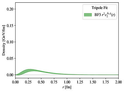
The subsection below lists the various densities computed for each hadron. In all expressions for the densities and radii, we use the definitions 2=1r2ddrr2ddrsuperscript21superscript𝑟2𝑑𝑑𝑟superscript𝑟2𝑑𝑑𝑟\partial^{2}=\frac{1}{r^{2}}\frac{d}{dr}r^{2}\frac{d}{dr} and 2=1rddrrddrsubscriptsuperscript2bottom1subscript𝑟bottom𝑑𝑑subscript𝑟bottomsubscript𝑟bottom𝑑𝑑subscript𝑟bottom\partial^{2}_{{\!\bot\!}}=\frac{1}{r_{{\!\bot\!}}}\frac{d}{dr_{{\!\bot\!}}}r_{{\!\bot\!}}\frac{d}{dr_{{\!\bot\!}}}, and the \approx symbol in the IMF definitions when suppressing higher-order terms in 𝒪(Pz)𝒪subscript𝑃𝑧\mathcal{O}(P_{z}). Moreover, the symbol X𝑋X is defined such that

X={6for BF38for BF2/IMF.𝑋cases6for BF3otherwise8for BF2/IMFotherwiseX=\begin{cases}6\quad\text{for BF3}\\ 8\quad\text{for BF2/IMF}\end{cases}\;. (65)

B.1 Pion

Below we list expressions for the BF energy (ϵitalic-ϵ\epsilon), pressure (p𝑝p), and shear force (s𝑠s) densities, and the mass radii of the pion [88, 33], as well as the contributions to the IMF densities and radii at lowest order in 𝒪(1/Pz)𝒪1subscript𝑃𝑧\mathcal{O}(1/P_{z}). The IMF densities are derived by considering the matrix elements γπ(𝐩)|Tg00|π(𝐩)𝛾bra𝜋superscript𝐩subscriptsuperscript𝑇00𝑔ket𝜋𝐩\gamma\bra{\pi({\mathbf{p}}^{\prime})}T^{00}_{g}\ket{\pi({\mathbf{p}})} and π(𝐩)|Tgij|π(𝐩)/γbra𝜋superscript𝐩subscriptsuperscript𝑇𝑖𝑗𝑔ket𝜋𝐩𝛾\bra{\pi({\mathbf{p}}^{\prime})}T^{ij}_{g}\ket{\pi({\mathbf{p}})}/\gamma, where γ𝛾\gamma is the relativistic boost factor.

εBF3(2)π,i(r())subscriptsuperscript𝜀𝜋𝑖BF3(2)subscript𝑟bottom\displaystyle\varepsilon^{\pi,i}_{\text{BF3(2)}}(r_{({\!\bot\!})}) =mπ2[1mπ2t/4(Aiπ(t)+c¯iπ(t)t4mπ2(Aiπ(t)+Diπ(t)))]BF3(2),absentsuperscriptsubscript𝑚𝜋2subscriptdelimited-[]1superscriptsubscript𝑚𝜋2𝑡4subscriptsuperscript𝐴𝜋𝑖𝑡subscriptsuperscript¯𝑐𝜋𝑖𝑡𝑡4superscriptsubscript𝑚𝜋2subscriptsuperscript𝐴𝜋𝑖𝑡subscriptsuperscript𝐷𝜋𝑖𝑡BF3(2)\displaystyle=m_{\pi}^{2}\left[\frac{1}{\sqrt{m_{\pi}^{2}-t/4}}\left(A^{\pi}_{i}(t)+\bar{c}^{\pi}_{i}(t)-\frac{t}{4m_{\pi}^{2}}(A^{\pi}_{i}(t)+D^{\pi}_{i}(t))\right)\right]_{\text{BF3(2)}}\;, (66)
pBF3(2)π,i(r())subscriptsuperscript𝑝𝜋𝑖BF3(2)subscript𝑟bottom\displaystyle p^{\pi,i}_{\text{BF3(2)}}(r_{({\!\bot\!})}) =1X()2[1mπ2t/4Diπ(t)]BF3(2)mπ2[1mπ2t/4c¯iπ(t)]BF3(2),absent1𝑋subscriptsuperscript2bottomsubscriptdelimited-[]1superscriptsubscript𝑚𝜋2𝑡4subscriptsuperscript𝐷𝜋𝑖𝑡BF3(2)superscriptsubscript𝑚𝜋2subscriptdelimited-[]1superscriptsubscript𝑚𝜋2𝑡4subscriptsuperscript¯𝑐𝜋𝑖𝑡BF3(2)\displaystyle=\frac{1}{X}\partial^{2}_{({\!\bot\!})}\left[\frac{1}{\sqrt{m_{\pi}^{2}-t/4}}D^{\pi}_{i}(t)\right]_{\text{BF3(2)}}-m_{\pi}^{2}\left[\frac{1}{\sqrt{m_{\pi}^{2}-t/4}}\bar{c}^{\pi}_{i}(t)\right]_{\text{BF3(2)}}\;, (67)
sBF3(2)π,i(r())subscriptsuperscript𝑠𝜋𝑖BF3(2)subscript𝑟bottom\displaystyle s^{\pi,i}_{\text{BF3(2)}}(r_{({\!\bot\!})}) =14r()ddr()1r()ddr()[1mπ2t/4Diπ(t)]BF3(2),absent14subscript𝑟bottom𝑑𝑑subscript𝑟bottom1subscript𝑟bottom𝑑𝑑subscript𝑟bottomsubscriptdelimited-[]1superscriptsubscript𝑚𝜋2𝑡4subscriptsuperscript𝐷𝜋𝑖𝑡BF3(2)\displaystyle=-\frac{1}{4}r_{({\!\bot\!})}\frac{d}{dr_{({\!\bot\!})}}\frac{1}{r_{({\!\bot\!})}}\frac{d}{dr_{({\!\bot\!})}}\left[\frac{1}{\sqrt{m_{\pi}^{2}-t/4}}D^{\pi}_{i}(t)\right]_{\text{BF3(2)}}\;, (68)
εIMFπ,i(r)subscriptsuperscript𝜀𝜋𝑖IMFsubscript𝑟bottom\displaystyle\varepsilon^{\pi,i}_{\text{IMF}}(r_{{\!\bot\!}}) m[Aiπ(t)]IMF,absent𝑚subscriptdelimited-[]subscriptsuperscript𝐴𝜋𝑖𝑡IMF\displaystyle\approx m[A^{\pi}_{i}(t)]_{\text{IMF}}\;, (69)
pIMFi(r)subscriptsuperscript𝑝𝑖IMFsubscript𝑟bottom\displaystyle p^{i}_{\text{IMF}}(r_{{\!\bot\!}}) 18mπ1rddrrddr[Diπ(t)]IMFmπ[c¯iπ(t)]IMF,absent18subscript𝑚𝜋1subscript𝑟bottom𝑑𝑑subscript𝑟bottomsubscript𝑟bottom𝑑𝑑subscript𝑟bottomsubscriptdelimited-[]subscriptsuperscript𝐷𝜋𝑖𝑡IMFsubscript𝑚𝜋subscriptdelimited-[]subscriptsuperscript¯𝑐𝜋𝑖𝑡IMF\displaystyle\approx\frac{1}{8m_{\pi}}\frac{1}{r_{{\!\bot\!}}}\frac{d}{dr_{{\!\bot\!}}}r_{{\!\bot\!}}\frac{d}{dr_{{\!\bot\!}}}\left[D^{\pi}_{i}(t)\right]_{\text{IMF}}-m_{\pi}\left[\bar{c}^{\pi}_{i}(t)\right]_{\text{IMF}}\;, (70)
sIMFi(r)subscriptsuperscript𝑠𝑖IMFsubscript𝑟bottom\displaystyle s^{i}_{\text{IMF}}(r_{{\!\bot\!}}) 14mπrddr1rddr[Diπ(t)]IMF,absent14subscript𝑚𝜋subscript𝑟bottom𝑑𝑑subscript𝑟bottom1subscript𝑟bottom𝑑𝑑subscript𝑟bottomsubscriptdelimited-[]subscriptsuperscript𝐷𝜋𝑖𝑡IMF\displaystyle\approx-\frac{1}{4m_{\pi}}r_{{\!\bot\!}}\frac{d}{dr_{{\!\bot\!}}}\frac{1}{r_{{\!\bot\!}}}\frac{d}{dr_{{\!\bot\!}}}\left[D^{\pi}_{i}(t)\right]_{\text{IMF}}\;, (71)
ri2BF3π,masssuperscriptsubscriptexpectationsubscriptsuperscript𝑟2𝑖BF3𝜋mass\displaystyle\braket{r^{2}_{i}}_{\text{BF3}}^{\pi,\text{mass}} =lim𝚫01mπ2t/4Δ2[12mπ2t/4π(p)|Ti00|π(p)|Δ0=0]\displaystyle=\lim_{{\mathbf{\Delta}}\rightarrow 0}-\frac{1}{\sqrt{m_{\pi}^{2}-t/4}}\nabla^{2}_{\Delta}\left[\frac{1}{2\sqrt{m_{\pi}^{2}-t/4}}\bra{\pi(p^{\prime})}T_{i}^{00}\ket{\pi(p)}\rvert_{\Delta_{0}=0}\right]
=6dAiπ(t)dt|t=034mπ2(Aiπ(0)+2Diπ(0)),\displaystyle=6\frac{dA^{\pi}_{i}(t)}{dt}\rvert_{t=0}-\frac{3}{4m_{\pi}^{2}}(A^{\pi}_{i}(0)+2D^{\pi}_{i}(0))\;, (72)
ri2BF2π,masssuperscriptsubscriptexpectationsubscriptsuperscript𝑟2𝑖BF2𝜋mass\displaystyle\braket{r^{2}_{i}}_{\text{BF2}}^{\pi,\text{mass}} =4dAiπ(t)dt|t=012mπ2(Aiπ(0)+2Diπ(0))=23ri2BF3π,mass,\displaystyle=4\frac{dA^{\pi}_{i}(t)}{dt}\rvert_{t=0}-\frac{1}{2m_{\pi}^{2}}(A^{\pi}_{i}(0)+2D^{\pi}_{i}(0))=\frac{2}{3}\braket{r^{2}_{i}}_{\text{BF3}}^{\pi,\text{mass}}\;, (73)
ri2IMFπ,masssuperscriptsubscriptexpectationsubscriptsuperscript𝑟2𝑖IMF𝜋mass\displaystyle\braket{r^{2}_{i}}_{\text{IMF}}^{\pi,\text{mass}} =𝑑rr2εIMFπ,i(r)𝑑rεIMFπ,i(r)=4dAiπ(t)dt|t=0.\displaystyle=\frac{\int dr_{{\!\bot\!}}r_{{\!\bot\!}}^{2}\varepsilon^{\pi,i}_{\text{IMF}}(r)}{\int dr_{{\!\bot\!}}\varepsilon^{\pi,i}_{\text{IMF}}(r)}=4\frac{dA^{\pi}_{i}(t)}{dt}\rvert_{t=0}\;. (74)

B.2 Nucleon

The BF [88] and lowest-order IMF [95] densities and mass radii of the nucleon can be expressed as

εBF3(2)N,i(r())subscriptsuperscript𝜀𝑁𝑖BF3(2)subscript𝑟bottom\displaystyle\varepsilon^{N,i}_{\text{BF3(2)}}(r_{({\!\bot\!})}) =mN[AiN(t)t4mN2(DiN(t)BiN(t))+c¯iN(t)]BF3(2),absentsubscript𝑚𝑁subscriptdelimited-[]subscriptsuperscript𝐴𝑁𝑖𝑡𝑡4superscriptsubscript𝑚𝑁2subscriptsuperscript𝐷𝑁𝑖𝑡subscriptsuperscript𝐵𝑁𝑖𝑡subscriptsuperscript¯𝑐𝑁𝑖𝑡BF3(2)\displaystyle=m_{N}\left[A^{N}_{i}(t)-\frac{t}{4m_{N}^{2}}(D^{N}_{i}(t)-B^{N}_{i}(t))+\bar{c}^{N}_{i}(t)\right]_{\text{BF3(2)}}\;, (75)
εIMFN,i(r)subscriptsuperscript𝜀𝑁𝑖IMFsubscript𝑟bottom\displaystyle\varepsilon^{N,i}_{\text{IMF}}(r_{{\!\bot\!}}) =mN[AiN(t)]IMF,absentsubscript𝑚𝑁subscriptdelimited-[]subscriptsuperscript𝐴𝑁𝑖𝑡IMF\displaystyle=m_{N}[A^{N}_{i}(t)]_{\text{IMF}}\;, (76)
pBF3(2)/(IMF)N,i(r())subscriptsuperscript𝑝𝑁𝑖BF3(2)/(IMF)subscript𝑟bottom\displaystyle p^{N,i}_{\text{BF3(2)/(IMF)}}(r_{({\!\bot\!})}) =1XmN()2[DiN(t)]BF3(2)/(IMF)m[c¯iN(t)]BF3(2)/(IMF),absent1𝑋subscript𝑚𝑁subscriptsuperscript2bottomsubscriptdelimited-[]subscriptsuperscript𝐷𝑁𝑖𝑡BF3(2)/(IMF)𝑚subscriptdelimited-[]subscriptsuperscript¯𝑐𝑁𝑖𝑡BF3(2)/(IMF)\displaystyle=\frac{1}{Xm_{N}}\partial^{2}_{({\!\bot\!})}[D^{N}_{i}(t)]_{\text{BF3(2)/(IMF)}}-m[\bar{c}^{N}_{i}(t)]_{\text{BF3(2)/(IMF)}}\;, (77)
sBF3(2/IMF)N,i(r())subscriptsuperscript𝑠𝑁𝑖BF3(2/IMF)subscript𝑟bottom\displaystyle s^{N,i}_{\text{BF3(2/IMF)}}(r_{({\!\bot\!})}) =14mNr()ddr()1r()ddr()[DiN(t)]BF3(2/IMF),absent14subscript𝑚𝑁subscript𝑟bottom𝑑𝑑subscript𝑟bottom1subscript𝑟bottom𝑑𝑑subscript𝑟bottomsubscriptdelimited-[]subscriptsuperscript𝐷𝑁𝑖𝑡BF3(2/IMF)\displaystyle=-\frac{1}{4m_{N}}r_{({\!\bot\!})}\frac{d}{dr_{({\!\bot\!})}}\frac{1}{r_{({\!\bot\!})}}\frac{d}{dr_{({\!\bot\!})}}[D^{N}_{i}(t)]_{\text{BF3(2/IMF)}}\;, (78)
ri2BF3N,masssuperscriptsubscriptexpectationsubscriptsuperscript𝑟2𝑖BF3𝑁mass\displaystyle\braket{r^{2}_{i}}_{\text{BF3}}^{N,\text{mass}} =6dAiN(t)dt|t=0+32mN2(BiN(0)DiN(0)),\displaystyle=6\frac{dA^{N}_{i}(t)}{dt}\rvert_{t=0}+\frac{3}{2m_{N}^{2}}(B^{N}_{i}(0)-D^{N}_{i}(0))\;, (79)
ri2BF2N,masssuperscriptsubscriptexpectationsubscriptsuperscript𝑟2𝑖BF2𝑁mass\displaystyle\braket{r^{2}_{i}}_{\text{BF2}}^{N,\text{mass}} =23ri2BF3N,mass,absent23superscriptsubscriptexpectationsubscriptsuperscript𝑟2𝑖BF3𝑁mass\displaystyle=\frac{2}{3}\braket{r^{2}_{i}}_{\text{BF3}}^{N,\text{mass}}\;, (80)
ri2IMFN,masssuperscriptsubscriptexpectationsubscriptsuperscript𝑟2𝑖IMF𝑁mass\displaystyle\braket{r^{2}_{i}}_{\text{IMF}}^{N,\text{mass}} =4dAiN(t)dt|t=0.\displaystyle=4\frac{dA^{N}_{i}(t)}{dt}\rvert_{t=0}\;. (81)

B.3 ρ𝜌\rho meson

The BF3 densities of the ρ𝜌\rho meson were derived in Refs. [48, 91] and can be expressed as

ε0,BF3ρ,i(r)superscriptsubscript𝜀0BF3𝜌𝑖𝑟\displaystyle\varepsilon_{0,\text{BF3}}^{\rho,i}(r) =mρ2[1mρ2t/4(A0ρ,i(t)+14f¯ρ,i(t)12c¯0ρ,i(t)\displaystyle=m_{\rho}^{2}\left[\frac{1}{\sqrt{m_{\rho}^{2}-t/4}}\left(A^{\rho,i}_{0}(t)+\frac{1}{4}\bar{f}^{\rho,i}(t)-\frac{1}{2}\bar{c}^{\rho,i}_{0}(t)\vphantom{\frac{t^{3}}{192m_{\rho}^{6}}}\right.\right.
+t12mρ2[5A0ρ,i(t)+3D0ρ,i(t)+4Jρ,i(t)2Eρ,i(t)+A1ρ,i(t)+12f¯ρ,i(t)+c¯0ρ,i(t)+12c¯1ρ,i(t)]𝑡12superscriptsubscript𝑚𝜌2delimited-[]5subscriptsuperscript𝐴𝜌𝑖0𝑡3subscriptsuperscript𝐷𝜌𝑖0𝑡4superscript𝐽𝜌𝑖𝑡2superscript𝐸𝜌𝑖𝑡subscriptsuperscript𝐴𝜌𝑖1𝑡12superscript¯𝑓𝜌𝑖𝑡subscriptsuperscript¯𝑐𝜌𝑖0𝑡12subscriptsuperscript¯𝑐𝜌𝑖1𝑡\displaystyle+\frac{t}{12m_{\rho}^{2}}[-5A^{\rho,i}_{0}(t)+3D^{\rho,i}_{0}(t)+4J^{\rho,i}(t)-2E^{\rho,i}(t)+A^{\rho,i}_{1}(t)+\frac{1}{2}\bar{f}^{\rho,i}(t)+\bar{c}^{\rho,i}_{0}(t)+\frac{1}{2}\bar{c}^{\rho,i}_{1}(t)]
t224mρ4[A0ρ,i(t)+D0ρ,i(t)+2Jρ,i(t)2Eρ,i(t)+A1ρ,i(t)+12D1ρ,i(t)+14c¯1ρ,i]superscript𝑡224superscriptsubscript𝑚𝜌4delimited-[]subscriptsuperscript𝐴𝜌𝑖0𝑡subscriptsuperscript𝐷𝜌𝑖0𝑡2superscript𝐽𝜌𝑖𝑡2superscript𝐸𝜌𝑖𝑡subscriptsuperscript𝐴𝜌𝑖1𝑡12subscriptsuperscript𝐷𝜌𝑖1𝑡14subscriptsuperscript¯𝑐𝜌𝑖1\displaystyle-\frac{t^{2}}{24m_{\rho}^{4}}[-A^{\rho,i}_{0}(t)+D^{\rho,i}_{0}(t)+2J^{\rho,i}(t)-2E^{\rho,i}(t)+A^{\rho,i}_{1}(t)+\frac{1}{2}D^{\rho,i}_{1}(t)+\frac{1}{4}\bar{c}^{\rho,i}_{1}]
+t3192mρ6[A1ρ,i(t)+D1ρ,i(t)])]BF3,\displaystyle\left.\left.+\frac{t^{3}}{192m_{\rho}^{6}}[A^{\rho,i}_{1}(t)+D^{\rho,i}_{1}(t)]\right)\right]_{\text{BF3}}\;, (82)
ε2,BF3ρ,i(r)superscriptsubscript𝜀2BF3𝜌𝑖𝑟\displaystyle\varepsilon_{2,\text{BF3}}^{\rho,i}(r) =r2ddr1rddr[1mρ2t/4(A0ρ,i(t)+2Jρ,i(t)Eρ,i(t)+12A1ρ,i(t)+14f¯ρ,i(t)+12c¯0ρ,i(t)+14c¯1ρ,i(t)\displaystyle=-\frac{r}{2}\frac{d}{dr}\frac{1}{r}\frac{d}{dr}\left[\frac{1}{\sqrt{m_{\rho}^{2}-t/4}}\left(-A^{\rho,i}_{0}(t)+2J^{\rho,i}(t)-E^{\rho,i}(t)+\frac{1}{2}A^{\rho,i}_{1}(t)+\frac{1}{4}\bar{f}^{\rho,i}(t)+\frac{1}{2}\bar{c}_{0}^{\rho,i}(t)+\frac{1}{4}\bar{c}_{1}^{\rho,i}(t)\vphantom{\frac{t}{4m_{\rho}^{2}}}\right.\right.
t4mρ2[A0ρ,i(t)+D0ρ,i(t)+2Jρ,i(t)2Eρ,i(t)+A1ρ,i(t)+12D1ρ,i(t)+14c¯1ρ,i(t)]𝑡4superscriptsubscript𝑚𝜌2delimited-[]subscriptsuperscript𝐴𝜌𝑖0𝑡subscriptsuperscript𝐷𝜌𝑖0𝑡2superscript𝐽𝜌𝑖𝑡2superscript𝐸𝜌𝑖𝑡subscriptsuperscript𝐴𝜌𝑖1𝑡12subscriptsuperscript𝐷𝜌𝑖1𝑡14subscriptsuperscript¯𝑐𝜌𝑖1𝑡\displaystyle-\frac{t}{4m_{\rho}^{2}}[-A^{\rho,i}_{0}(t)+D^{\rho,i}_{0}(t)+2J^{\rho,i}(t)-2E^{\rho,i}(t)+A^{\rho,i}_{1}(t)+\frac{1}{2}D^{\rho,i}_{1}(t)+\frac{1}{4}\bar{c}^{\rho,i}_{1}(t)]
+t232mρ4[A1ρ,i(t)+D1ρ,i(t)])]BF3,\displaystyle\left.\left.+\frac{t^{2}}{32m_{\rho}^{4}}[A^{\rho,i}_{1}(t)+D^{\rho,i}_{1}(t)]\right)\right]_{\text{BF3}}\;, (83)
p0,BF3ρ,i(r)superscriptsubscript𝑝0BF3𝜌𝑖𝑟\displaystyle p_{0,\text{BF3}}^{\rho,i}(r) =162[1mρ2t/4(D0ρ,i(t)+43Eρ,i(t)+t12mρ2[2D0ρ,i(t)2Eρ,i(t)+D1ρ,i(t)]t248mρ4D1ρ,i(t))]BF3,absent16superscript2subscriptdelimited-[]1superscriptsubscript𝑚𝜌2𝑡4subscriptsuperscript𝐷𝜌𝑖0𝑡43superscript𝐸𝜌𝑖𝑡𝑡12superscriptsubscript𝑚𝜌2delimited-[]2subscriptsuperscript𝐷𝜌𝑖0𝑡2superscript𝐸𝜌𝑖𝑡subscriptsuperscript𝐷𝜌𝑖1𝑡superscript𝑡248superscriptsubscript𝑚𝜌4subscriptsuperscript𝐷𝜌𝑖1𝑡BF3\displaystyle=\frac{1}{6}\partial^{2}\left[\frac{1}{\sqrt{m_{\rho}^{2}-t/4}}\left(-D^{\rho,i}_{0}(t)+\frac{4}{3}E^{\rho,i}(t)+\frac{t}{12m_{\rho}^{2}}[2D^{\rho,i}_{0}(t)-2E^{\rho,i}(t)+D^{\rho,i}_{1}(t)]-\frac{t^{2}}{48m_{\rho}^{4}}D^{\rho,i}_{1}(t)\right)\right]_{\text{BF3}}\;, (84)
p2,BF3ρ,i(r)superscriptsubscript𝑝2BF3𝜌𝑖𝑟\displaystyle p_{2,\text{BF3}}^{\rho,i}(r) =162[Eρ,i(t)mρ2t/4]BF3absent16superscript2subscriptdelimited-[]superscript𝐸𝜌𝑖𝑡superscriptsubscript𝑚𝜌2𝑡4BF3\displaystyle=\frac{1}{6}\partial^{2}\left[\frac{-E^{\rho,i}(t)}{\sqrt{m_{\rho}^{2}-t/4}}\right]_{\text{BF3}}
+16mρ2(ddrddr2rddr)[1mρ2t/4(12D0ρ,i(t)12Eρ,i(t)+14D1ρ,i(t)t16mρ2D1ρ,i(t))]BF3,16subscript𝑚𝜌superscript2𝑑𝑑𝑟𝑑𝑑𝑟2𝑟𝑑𝑑𝑟subscriptdelimited-[]1superscriptsubscript𝑚𝜌2𝑡412subscriptsuperscript𝐷𝜌𝑖0𝑡12superscript𝐸𝜌𝑖𝑡14subscriptsuperscript𝐷𝜌𝑖1𝑡𝑡16superscriptsubscript𝑚𝜌2subscriptsuperscript𝐷𝜌𝑖1𝑡BF3\displaystyle+\frac{1}{6m_{\rho}}\partial^{2}\left(\frac{d}{dr}\frac{d}{dr}-\frac{2}{r}\frac{d}{dr}\right)\left[\frac{1}{\sqrt{m_{\rho}^{2}-t/4}}\left(\frac{1}{2}D^{\rho,i}_{0}(t)-\frac{1}{2}E^{\rho,i}(t)+\frac{1}{4}D^{\rho,i}_{1}(t)-\frac{t}{16m_{\rho}^{2}}D^{\rho,i}_{1}(t)\right)\right]_{\text{BF3}}\;, (85)
p3,BF3ρ,i(r)superscriptsubscript𝑝3BF3𝜌𝑖𝑟\displaystyle p_{3,\text{BF3}}^{\rho,i}(r) =26mρ2(ddrddr3rddr)absent26subscript𝑚𝜌superscript2𝑑𝑑𝑟𝑑𝑑𝑟3𝑟𝑑𝑑𝑟\displaystyle=-\frac{2}{6m_{\rho}}\partial^{2}\left(\frac{d}{dr}\frac{d}{dr}-\frac{3}{r}\frac{d}{dr}\right)
[1mρ2t/4(12D0ρ,i(t)12Eρ,i(t)+14D1ρ,i(t)t16mρ2D1ρ,i(t))]BF3,subscriptdelimited-[]1superscriptsubscript𝑚𝜌2𝑡412subscriptsuperscript𝐷𝜌𝑖0𝑡12superscript𝐸𝜌𝑖𝑡14subscriptsuperscript𝐷𝜌𝑖1𝑡𝑡16superscriptsubscript𝑚𝜌2subscriptsuperscript𝐷𝜌𝑖1𝑡BF3\displaystyle\left[\frac{1}{\sqrt{m_{\rho}^{2}-t/4}}\left(\frac{1}{2}D^{\rho,i}_{0}(t)-\frac{1}{2}E^{\rho,i}(t)+\frac{1}{4}D^{\rho,i}_{1}(t)-\frac{t}{16m_{\rho}^{2}}D^{\rho,i}_{1}(t)\right)\right]_{\text{BF3}}\;, (86)
s0,BF3ρ,i(t)superscriptsubscript𝑠0BF3𝜌𝑖𝑡\displaystyle s_{0,\text{BF3}}^{\rho,i}(t) =14rddr1rddrabsent14𝑟𝑑𝑑𝑟1𝑟𝑑𝑑𝑟\displaystyle=-\frac{1}{4}r\frac{d}{dr}\frac{1}{r}\frac{d}{dr}
[1mρ2t/4(D0ρ,i(t)+43Eρ,i(t)+t12mρ2[2D0ρ,i(t)2Eρ,i(t)+D1ρ,i(t)]t248mρ4D1ρ,i(t))]BF3,subscriptdelimited-[]1superscriptsubscript𝑚𝜌2𝑡4subscriptsuperscript𝐷𝜌𝑖0𝑡43superscript𝐸𝜌𝑖𝑡𝑡12superscriptsubscript𝑚𝜌2delimited-[]2subscriptsuperscript𝐷𝜌𝑖0𝑡2superscript𝐸𝜌𝑖𝑡subscriptsuperscript𝐷𝜌𝑖1𝑡superscript𝑡248superscriptsubscript𝑚𝜌4subscriptsuperscript𝐷𝜌𝑖1𝑡BF3\displaystyle\left[\frac{1}{\sqrt{m_{\rho}^{2}-t/4}}\left(-D^{\rho,i}_{0}(t)+\frac{4}{3}E^{\rho,i}(t)+\frac{t}{12m_{\rho}^{2}}[2D^{\rho,i}_{0}(t)-2E^{\rho,i}(t)+D^{\rho,i}_{1}(t)]-\frac{t^{2}}{48m_{\rho}^{4}}D^{\rho,i}_{1}(t)\right)\right]_{\text{BF3}}\;, (87)
s2,BF3ρ,i(r)superscriptsubscript𝑠2BF3𝜌𝑖𝑟\displaystyle s_{2,\text{BF3}}^{\rho,i}(r) =14rddr1rddr[Eρ,i(t)mρ2t/4]BF3absent14𝑟𝑑𝑑𝑟1𝑟𝑑𝑑𝑟subscriptdelimited-[]superscript𝐸𝜌𝑖𝑡superscriptsubscript𝑚𝜌2𝑡4BF3\displaystyle=-\frac{1}{4}r\frac{d}{dr}\frac{1}{r}\frac{d}{dr}\left[\frac{-E^{\rho,i}(t)}{\sqrt{m_{\rho}^{2}-t/4}}\right]_{\text{BF3}}
14mρrddr1rddr(ddrddr2rddr)14subscript𝑚𝜌𝑟𝑑𝑑𝑟1𝑟𝑑𝑑𝑟𝑑𝑑𝑟𝑑𝑑𝑟2𝑟𝑑𝑑𝑟\displaystyle-\frac{1}{4m_{\rho}}r\frac{d}{dr}\frac{1}{r}\frac{d}{dr}\left(\frac{d}{dr}\frac{d}{dr}-\frac{2}{r}\frac{d}{dr}\right)
[1mρ2t/4(12D0ρ,i(t)12Eρ,i(t)+14D1ρ,i(t)t16mρ2D1ρ,i(t))]BF3,subscriptdelimited-[]1superscriptsubscript𝑚𝜌2𝑡412subscriptsuperscript𝐷𝜌𝑖0𝑡12superscript𝐸𝜌𝑖𝑡14subscriptsuperscript𝐷𝜌𝑖1𝑡𝑡16superscriptsubscript𝑚𝜌2subscriptsuperscript𝐷𝜌𝑖1𝑡BF3\displaystyle\left[\frac{1}{\sqrt{m_{\rho}^{2}-t/4}}\left(\frac{1}{2}D^{\rho,i}_{0}(t)-\frac{1}{2}E^{\rho,i}(t)+\frac{1}{4}D^{\rho,i}_{1}(t)-\frac{t}{16m_{\rho}^{2}}D^{\rho,i}_{1}(t)\right)\right]_{\text{BF3}}\;, (88)
s3,BF3ρ,i(r)superscriptsubscript𝑠3BF3𝜌𝑖𝑟\displaystyle s_{3,\text{BF3}}^{\rho,i}(r) =12mρrddr1rddr(ddrddr3rddr)absent12subscript𝑚𝜌𝑟𝑑𝑑𝑟1𝑟𝑑𝑑𝑟𝑑𝑑𝑟𝑑𝑑𝑟3𝑟𝑑𝑑𝑟\displaystyle=\frac{1}{2m_{\rho}}r\frac{d}{dr}\frac{1}{r}\frac{d}{dr}\left(\frac{d}{dr}\frac{d}{dr}-\frac{3}{r}\frac{d}{dr}\right)
[1mρ2t/4(12D0ρ,i(t)12Eρ,i(t)+14D1ρ,i(t)t16mρ2D1ρ,i(t))]BF3.subscriptdelimited-[]1superscriptsubscript𝑚𝜌2𝑡412subscriptsuperscript𝐷𝜌𝑖0𝑡12superscript𝐸𝜌𝑖𝑡14subscriptsuperscript𝐷𝜌𝑖1𝑡𝑡16superscriptsubscript𝑚𝜌2subscriptsuperscript𝐷𝜌𝑖1𝑡BF3\displaystyle\left[\frac{1}{\sqrt{m_{\rho}^{2}-t/4}}\left(\frac{1}{2}D^{\rho,i}_{0}(t)-\frac{1}{2}E^{\rho,i}(t)+\frac{1}{4}D^{\rho,i}_{1}(t)-\frac{t}{16m_{\rho}^{2}}D^{\rho,i}_{1}(t)\right)\right]_{\text{BF3}}\;. (89)

Using the same methods but restricting the analysis to a two-dimensional plane, we obtain the following expressions for the BF2 leading-order contributions to the EMT monopole densities:

ε0,BF2ρ,i(r)superscriptsubscript𝜀0BF2𝜌𝑖subscript𝑟bottom\displaystyle\varepsilon_{0,\text{BF2}}^{\rho,i}(r_{{\!\bot\!}}) =mρ2[1mρ2t/4(A0ρ,i(t)+14f¯ρ,i(t)12c¯0ρ,i(t)\displaystyle=m_{\rho}^{2}\left[\frac{1}{\sqrt{m_{\rho}^{2}-t/4}}\left(A^{\rho,i}_{0}(t)+\frac{1}{4}\bar{f}^{\rho,i}(t)-\frac{1}{2}\bar{c}^{\rho,i}_{0}(t)\vphantom{\frac{t}{8m_{\rho}^{2}}}\right.\right.
+t8mρ2[4A0ρ,i(t)+2D0ρ,i(t)+4Jρ,i(t)2Eρ,i(t)+A1ρ,i(t)+12f¯ρ,i(t)+c¯0ρ,i(t)+12c¯1ρ,i(t)]𝑡8superscriptsubscript𝑚𝜌2delimited-[]4subscriptsuperscript𝐴𝜌𝑖0𝑡2subscriptsuperscript𝐷𝜌𝑖0𝑡4superscript𝐽𝜌𝑖𝑡2superscript𝐸𝜌𝑖𝑡subscriptsuperscript𝐴𝜌𝑖1𝑡12superscript¯𝑓𝜌𝑖𝑡subscriptsuperscript¯𝑐𝜌𝑖0𝑡12subscriptsuperscript¯𝑐𝜌𝑖1𝑡\displaystyle+\frac{t}{8m_{\rho}^{2}}[-4A^{\rho,i}_{0}(t)+2D^{\rho,i}_{0}(t)+4J^{\rho,i}(t)-2E^{\rho,i}(t)+A^{\rho,i}_{1}(t)+\frac{1}{2}\bar{f}^{\rho,i}(t)+\bar{c}^{\rho,i}_{0}(t)+\frac{1}{2}\bar{c}^{\rho,i}_{1}(t)]
+t216mρ4[A0ρ,i(t)D0ρ,i(t)2Jρ,i(t)+2Eρ,i(t)A1ρ,i(t)12D1ρ,i(t)14c¯1ρ,i(t)]superscript𝑡216superscriptsubscript𝑚𝜌4delimited-[]subscriptsuperscript𝐴𝜌𝑖0𝑡subscriptsuperscript𝐷𝜌𝑖0𝑡2superscript𝐽𝜌𝑖𝑡2superscript𝐸𝜌𝑖𝑡subscriptsuperscript𝐴𝜌𝑖1𝑡12subscriptsuperscript𝐷𝜌𝑖1𝑡14subscriptsuperscript¯𝑐𝜌𝑖1𝑡\displaystyle+\frac{t^{2}}{16m_{\rho}^{4}}[A^{\rho,i}_{0}(t)-D^{\rho,i}_{0}(t)-2J^{\rho,i}(t)+2E^{\rho,i}(t)-A^{\rho,i}_{1}(t)-\frac{1}{2}D^{\rho,i}_{1}(t)-\frac{1}{4}\bar{c}^{\rho,i}_{1}(t)]
+t3128mρ6[A1ρ,i(t)+D1ρ,i(t)])]BF2,\displaystyle\left.\left.+\frac{t^{3}}{128m_{\rho}^{6}}[A^{\rho,i}_{1}(t)+D^{\rho,i}_{1}(t)]\right)\right]_{\text{BF2}}\;, (90)
s0,BF2ρ,i(r)subscriptsuperscript𝑠𝜌𝑖0BF2subscript𝑟bottom\displaystyle s^{\rho,i}_{0,\text{BF2}}(r_{{\!\bot\!}}) =14rddr1rddrabsent14subscript𝑟bottom𝑑𝑑subscript𝑟bottom1subscript𝑟bottom𝑑𝑑subscript𝑟bottom\displaystyle=-\frac{1}{4}r_{{\!\bot\!}}\frac{d}{dr_{{\!\bot\!}}}\frac{1}{r_{{\!\bot\!}}}\frac{d}{dr_{{\!\bot\!}}}
[1mρ2t/4(D0ρ,i(t)+2Eρ,i(t)+t4mρ2(D0ρ,i(t)+12D1ρ,i(t)Eρ,i(t))t232mρ4D1ρ,i(t))]BF2,subscriptdelimited-[]1superscriptsubscript𝑚𝜌2𝑡4superscriptsubscript𝐷0𝜌𝑖𝑡2superscript𝐸𝜌𝑖𝑡𝑡4superscriptsubscript𝑚𝜌2superscriptsubscript𝐷0𝜌𝑖𝑡12superscriptsubscript𝐷1𝜌𝑖𝑡superscript𝐸𝜌𝑖𝑡superscript𝑡232superscriptsubscript𝑚𝜌4superscriptsubscript𝐷1𝜌𝑖𝑡BF2\displaystyle\left[\frac{1}{\sqrt{m_{\rho}^{2}-t/4}}\left(-D_{0}^{\rho,i}(t)+2E^{\rho,i}(t)+\frac{t}{4m_{\rho}^{2}}(D_{0}^{\rho,i}(t)+\frac{1}{2}D_{1}^{\rho,i}(t)-E^{\rho,i}(t))-\frac{t^{2}}{32m_{\rho}^{4}}D_{1}^{\rho,i}(t)\right)\right]_{\text{BF2}}\;, (91)
p0,BF2ρ,i(r)subscriptsuperscript𝑝𝜌𝑖0BF2subscript𝑟bottom\displaystyle p^{\rho,i}_{0,\text{BF2}}(r_{{\!\bot\!}}) =182[1mρ2t/4(D0ρ,i(t)+2Eρ,i(t)+t4mρ2(D0ρ,i(t)+12D1ρ,i(t)Eρ,i(t))t232mρ4D1ρ,i(t))]BF2.absent18subscriptsuperscript2bottomsubscriptdelimited-[]1superscriptsubscript𝑚𝜌2𝑡4subscriptsuperscript𝐷𝜌𝑖0𝑡2superscript𝐸𝜌𝑖𝑡𝑡4superscriptsubscript𝑚𝜌2superscriptsubscript𝐷0𝜌𝑖𝑡12superscriptsubscript𝐷1𝜌𝑖𝑡superscript𝐸𝜌𝑖𝑡superscript𝑡232superscriptsubscript𝑚𝜌4superscriptsubscript𝐷1𝜌𝑖𝑡BF2\displaystyle=\frac{1}{8}\partial^{2}_{{\!\bot\!}}\left[\frac{1}{\sqrt{m_{\rho}^{2}-t/4}}\left(-D^{\rho,i}_{0}(t)+2E^{\rho,i}(t)+\frac{t}{4m_{\rho}^{2}}(D_{0}^{\rho,i}(t)+\frac{1}{2}D_{1}^{\rho,i}(t)-E^{\rho,i}(t))-\frac{t^{2}}{32m_{\rho}^{4}}D_{1}^{\rho,i}(t)\right)\right]_{\text{BF2}}\;. (92)

By considering the matrix elements γρ(p,s)|Tg00|ρ(p,s)𝛾bra𝜌superscript𝑝superscript𝑠subscriptsuperscript𝑇00𝑔ket𝜌𝑝𝑠\gamma\bra{\rho(p^{\prime},s^{\prime})}T^{00}_{g}\ket{\rho(p,s)} and ρ(p,s)|Tgij|ρ(p,s)/γbra𝜌superscript𝑝superscript𝑠subscriptsuperscript𝑇𝑖𝑗𝑔ket𝜌𝑝𝑠𝛾\bra{\rho(p^{\prime},s^{\prime})}T^{ij}_{g}\ket{\rho(p,s)}/\gamma, we obtain the lowest-order contributions to the monopole densities in the IMF as

ε0,IMFρ,i(r)subscriptsuperscript𝜀𝜌𝑖0IMFsubscript𝑟bottom\displaystyle\varepsilon^{\rho,i}_{0,\text{IMF}}(r_{{\!\bot\!}}) mρ[A0ρ,i(t)]IMF,absentsubscript𝑚𝜌subscriptdelimited-[]subscriptsuperscript𝐴𝜌𝑖0𝑡IMF\displaystyle\approx m_{\rho}[A^{\rho,i}_{0}(t)]_{\text{IMF}}\;, (93)
s0,IMFρ,i(r)subscriptsuperscript𝑠𝜌𝑖0IMFsubscript𝑟bottom\displaystyle s^{\rho,i}_{0,\text{IMF}}(r_{{\!\bot\!}}) 14mρrddr1rddr[D0ρ,i(t)+2Eρ,i(t)]IMF,absent14subscript𝑚𝜌subscript𝑟bottom𝑑𝑑subscript𝑟bottom1subscript𝑟bottom𝑑𝑑subscript𝑟bottomsubscriptdelimited-[]superscriptsubscript𝐷0𝜌𝑖𝑡2superscript𝐸𝜌𝑖𝑡IMF\displaystyle\approx-\frac{1}{4m_{\rho}}r_{{\!\bot\!}}\frac{d}{dr_{{\!\bot\!}}}\frac{1}{r_{{\!\bot\!}}}\frac{d}{dr_{{\!\bot\!}}}[-D_{0}^{\rho,i}(t)+2E^{\rho,i}(t)]_{\text{IMF}}\;, (94)
p0,IMFρ,i(r)subscriptsuperscript𝑝𝜌𝑖0IMFsubscript𝑟bottom\displaystyle p^{\rho,i}_{0,\text{IMF}}(r_{{\!\bot\!}}) 18mρ2[D0ρ,i(t)+2Eρ,i(t)]IMF.absent18subscript𝑚𝜌subscriptsuperscript2bottomsubscriptdelimited-[]subscriptsuperscript𝐷𝜌𝑖0𝑡2superscript𝐸𝜌𝑖𝑡IMF\displaystyle\approx\frac{1}{8m_{\rho}}\partial^{2}_{{\!\bot\!}}[-D^{\rho,i}_{0}(t)+2E^{\rho,i}(t)]_{\text{IMF}}\,. (95)

The corresponding conserved mass radii are

ri2BF3ρ,masssuperscriptsubscriptexpectationsubscriptsuperscript𝑟2𝑖BF3𝜌mass\displaystyle\braket{r^{2}_{i}}_{\text{BF3}}^{\rho,\text{mass}} =6dA0ρ,i(t)dt|t=0+1mρ2(74A0ρ,i(0)+12A1ρ,i(0)+32D0ρ,i(t)+2Jρ,i(0)Eρ,i(0)),\displaystyle=6\frac{dA^{\rho,i}_{0}(t)}{dt}\rvert_{t=0}+\frac{1}{m_{\rho}^{2}}(-\frac{7}{4}A^{\rho,i}_{0}(0)+\frac{1}{2}A^{\rho,i}_{1}(0)+\frac{3}{2}D^{\rho,i}_{0}(t)+2J^{\rho,i}(0)-E^{\rho,i}(0))\;, (96)
ri2BF2ρ,masssuperscriptsubscriptexpectationsubscriptsuperscript𝑟2𝑖BF2𝜌mass\displaystyle\braket{r^{2}_{i}}_{\text{BF2}}^{\rho,\text{mass}} =4dA0ρ,i(t)dt|t=0+12mρ2(4A0ρ,i(0)+A1ρ,i(0)+2D0ρ,i(0)2Eρ,i(0)+4Jρ,i(0)),\displaystyle=4\frac{dA^{\rho,i}_{0}(t)}{dt}\rvert_{t=0}+\frac{1}{2m_{\rho}^{2}}(-4A^{\rho,i}_{0}(0)+A^{\rho,i}_{1}(0)+2D^{\rho,i}_{0}(0)-2E^{\rho,i}(0)+4J^{\rho,i}(0))\;, (97)
ri2IMFρ,masssuperscriptsubscriptexpectationsubscriptsuperscript𝑟2𝑖IMF𝜌mass\displaystyle\braket{r^{2}_{i}}_{\text{IMF}}^{\rho,\text{mass}} =4dA0ρ,i(t)dt|t=0.\displaystyle=4\frac{dA^{\rho,i}_{0}(t)}{dt}\rvert_{t=0}\,. (98)

Note that the IMF energy density corresponds to a different component of the EMT than the Drell-Yan frame (DYF) energy, as discussed in Ref. [95] for the case of the nucleon, and therefore the IMF mass radius is different than the DYF radius found in Ref. [33].

B.4 ΔΔ\Delta baryon

The BF3 densities of the ΔΔ\Delta baryon were derived in Ref. [37] and are

ε0,BF3Δ,i(r)superscriptsubscript𝜀0BF3Δ𝑖𝑟\displaystyle\varepsilon_{0,\text{BF3}}^{\Delta,i}(r) =mΔ[F10Δ,i(t)+F30Δ,i(t)\displaystyle=m_{\Delta}\bigg{[}F^{\Delta,i}_{10}(t)+F^{\Delta,i}_{30}(t)
+t6mΔ2(52F10Δ,i(t)F11Δ,i(t)32F20Δ,i(t)+4F50Δ,i(t)+3F40Δ,i(t)F30Δ,i(t)F31Δ,i(t)F60Δ,i(t))𝑡6superscriptsubscript𝑚Δ252subscriptsuperscript𝐹Δ𝑖10𝑡subscriptsuperscript𝐹Δ𝑖11𝑡32subscriptsuperscript𝐹Δ𝑖20𝑡4subscriptsuperscript𝐹Δ𝑖50𝑡3subscriptsuperscript𝐹Δ𝑖40𝑡subscriptsuperscript𝐹Δ𝑖30𝑡subscriptsuperscript𝐹Δ𝑖31𝑡subscriptsuperscript𝐹Δ𝑖60𝑡\displaystyle+\frac{t}{6m_{\Delta}^{2}}\left(-\frac{5}{2}F^{\Delta,i}_{10}(t)-F^{\Delta,i}_{11}(t)-\frac{3}{2}F^{\Delta,i}_{20}(t)+4F^{\Delta,i}_{50}(t)+3F^{\Delta,i}_{40}(t)-F^{\Delta,i}_{30}(t)-F^{\Delta,i}_{31}(t)-F^{\Delta,i}_{60}(t)\right)
+t212mΔ4(12F10Δ,i(t)+F11Δ,i(t)+12F20Δ,i(t)+12F21Δ,i(t)4F50Δ,i(t)F40Δ,i(t)F41Δ,i(t)+12F31Δ,i(t))superscript𝑡212superscriptsubscript𝑚Δ412subscriptsuperscript𝐹Δ𝑖10𝑡subscriptsuperscript𝐹Δ𝑖11𝑡12subscriptsuperscript𝐹Δ𝑖20𝑡12subscriptsuperscript𝐹Δ𝑖21𝑡4subscriptsuperscript𝐹Δ𝑖50𝑡subscriptsuperscript𝐹Δ𝑖40𝑡subscriptsuperscript𝐹Δ𝑖41𝑡12subscriptsuperscript𝐹Δ𝑖31𝑡\displaystyle+\frac{t^{2}}{12m_{\Delta}^{4}}\left(\frac{1}{2}F^{\Delta,i}_{10}(t)+F^{\Delta,i}_{11}(t)+\frac{1}{2}F^{\Delta,i}_{20}(t)+\frac{1}{2}F^{\Delta,i}_{21}(t)-4F^{\Delta,i}_{50}(t)-F^{\Delta,i}_{40}(t)-F^{\Delta,i}_{41}(t)+\frac{1}{2}F^{\Delta,i}_{31}(t)\right)
+t348mΔ6(12F11Δ,i(t)12F21Δ,i(t)+F41Δ,i(t))]BF3\displaystyle+\frac{t^{3}}{48m_{\Delta}^{6}}\left(-\frac{1}{2}F^{\Delta,i}_{11}(t)-\frac{1}{2}F^{\Delta,i}_{21}(t)+F^{\Delta,i}_{41}(t)\right)\bigg{]}_{\text{BF3}} (99)
ε2,BF3Δ,i(r)superscriptsubscript𝜀2BF3Δ𝑖𝑟\displaystyle\varepsilon_{2,\text{BF3}}^{\Delta,i}(r) =1mΔr()ddr1rddr[16(F10Δ,i(t)+F11Δ,i(t)4F50Δ,i(t)+F30Δ,i(t)+F31Δ,i(t)+F60Δ,i(t))\displaystyle=-\frac{1}{m_{\Delta}}r_{({\!\bot\!})}\frac{d}{dr}\frac{1}{r}\frac{d}{dr}\bigg{[}-\frac{1}{6}\left(F^{\Delta,i}_{10}(t)+F^{\Delta,i}_{11}(t)-4F^{\Delta,i}_{50}(t)+F^{\Delta,i}_{30}(t)+F^{\Delta,i}_{31}(t)+F^{\Delta,i}_{60}(t)\right)
+t12mΔ2(12F10Δ,i(t)+F11Δ,i(t)+12F20Δ,i(t)+12F21Δ,i(t)4F50Δ,i(t)F40Δ,i(t)F41Δ,i(t)+12F31Δ,i(t))𝑡12superscriptsubscript𝑚Δ212subscriptsuperscript𝐹Δ𝑖10𝑡subscriptsuperscript𝐹Δ𝑖11𝑡12subscriptsuperscript𝐹Δ𝑖20𝑡12subscriptsuperscript𝐹Δ𝑖21𝑡4subscriptsuperscript𝐹Δ𝑖50𝑡subscriptsuperscript𝐹Δ𝑖40𝑡subscriptsuperscript𝐹Δ𝑖41𝑡12subscriptsuperscript𝐹Δ𝑖31𝑡\displaystyle+\frac{t}{12m_{\Delta}^{2}}\left(\frac{1}{2}F^{\Delta,i}_{10}(t)+F^{\Delta,i}_{11}(t)+\frac{1}{2}F^{\Delta,i}_{20}(t)+\frac{1}{2}F^{\Delta,i}_{21}(t)-4F^{\Delta,i}_{50}(t)-F^{\Delta,i}_{40}(t)-F^{\Delta,i}_{41}(t)+\frac{1}{2}F^{\Delta,i}_{31}(t)\right)
+t248mΔ4(12F11Δ,i(t)12F21Δ,i(t)+F41Δ,i(t))]BF3\displaystyle+\frac{t^{2}}{48m_{\Delta}^{4}}\left(-\frac{1}{2}F^{\Delta,i}_{11}(t)-\frac{1}{2}F^{\Delta,i}_{21}(t)+F^{\Delta,i}_{41}(t)\right)\bigg{]}_{\text{BF3}} (100)
p0,BF3Δ,i(r)superscriptsubscript𝑝0BF3Δ𝑖𝑟\displaystyle p_{0,\text{BF3}}^{\Delta,i}(r) =16mΔ2[F20Δ,i(t)163F50Δ,i(t)t6mΔ2(F20Δ,i(t)+F21Δ,i(t)4F50Δ,i(t))+t224mΔ4F21Δ,i(t)]BF3absent16subscript𝑚Δsuperscript2subscriptdelimited-[]subscriptsuperscript𝐹Δ𝑖20𝑡163subscriptsuperscript𝐹Δ𝑖50𝑡𝑡6superscriptsubscript𝑚Δ2subscriptsuperscript𝐹Δ𝑖20𝑡subscriptsuperscript𝐹Δ𝑖21𝑡4subscriptsuperscript𝐹Δ𝑖50𝑡superscript𝑡224superscriptsubscript𝑚Δ4subscriptsuperscript𝐹Δ𝑖21𝑡BF3\displaystyle=\frac{1}{6m_{\Delta}}\partial^{2}\bigg{[}F^{\Delta,i}_{20}(t)-\frac{16}{3}F^{\Delta,i}_{50}(t)-\frac{t}{6m_{\Delta}^{2}}\left(F^{\Delta,i}_{20}(t)+F^{\Delta,i}_{21}(t)-4F^{\Delta,i}_{50}(t)\right)+\frac{t^{2}}{24m_{\Delta}^{4}}F^{\Delta,i}_{21}(t)\bigg{]}_{\text{BF3}} (101)
p2,BF3Δ,i(r)superscriptsubscript𝑝2BF3Δ𝑖𝑟\displaystyle p_{2,\text{BF3}}^{\Delta,i}(r) =16mΔ2[43F50Δ,i(t)]BF3absent16subscript𝑚Δsuperscript2subscriptdelimited-[]43subscriptsuperscript𝐹Δ𝑖50𝑡BF3\displaystyle=\frac{1}{6m_{\Delta}}\partial^{2}\bigg{[}\frac{4}{3}F^{\Delta,i}_{50}(t)\bigg{]}_{\text{BF3}}
+\displaystyle+ 16mΔ22(ddrddr2rddr)[16(F20Δ,i(t)F21Δ,i(t)+4F50Δ,i(t))+t24mΔ2F21Δ,i(t)]BF316superscriptsubscript𝑚Δ2superscript2𝑑𝑑𝑟𝑑𝑑𝑟2𝑟𝑑𝑑𝑟subscriptdelimited-[]16subscriptsuperscript𝐹Δ𝑖20𝑡subscriptsuperscript𝐹Δ𝑖21𝑡4subscriptsuperscript𝐹Δ𝑖50𝑡𝑡24superscriptsubscript𝑚Δ2subscriptsuperscript𝐹Δ𝑖21𝑡BF3\displaystyle\frac{1}{6m_{\Delta}^{2}}\partial^{2}\left(\frac{d}{dr}\frac{d}{dr}-\frac{2}{r}\frac{d}{dr}\right)\bigg{[}\frac{1}{6}\left(-F^{\Delta,i}_{20}(t)-F^{\Delta,i}_{21}(t)+4F^{\Delta,i}_{50}(t)\right)+\frac{t}{24m_{\Delta}^{2}}F^{\Delta,i}_{21}(t)\bigg{]}_{\text{BF3}} (102)
p3,BF3Δ,i(r)superscriptsubscript𝑝3BF3Δ𝑖𝑟\displaystyle p_{3,\text{BF3}}^{\Delta,i}(r) =26mΔ22(ddrddr3rddr)[16(F20Δ,i(t)F21Δ,i(t)+4F50Δ,i(t))+t24mΔ2F21Δ,i(t)]BF3absent26superscriptsubscript𝑚Δ2superscript2𝑑𝑑𝑟𝑑𝑑𝑟3𝑟𝑑𝑑𝑟subscriptdelimited-[]16subscriptsuperscript𝐹Δ𝑖20𝑡subscriptsuperscript𝐹Δ𝑖21𝑡4subscriptsuperscript𝐹Δ𝑖50𝑡𝑡24superscriptsubscript𝑚Δ2subscriptsuperscript𝐹Δ𝑖21𝑡BF3\displaystyle=-\frac{2}{6m_{\Delta}^{2}}\partial^{2}\left(\frac{d}{dr}\frac{d}{dr}-\frac{3}{r}\frac{d}{dr}\right)\bigg{[}\frac{1}{6}\left(-F^{\Delta,i}_{20}(t)-F^{\Delta,i}_{21}(t)+4F^{\Delta,i}_{50}(t)\right)+\frac{t}{24m_{\Delta}^{2}}F^{\Delta,i}_{21}(t)\bigg{]}_{\text{BF3}} (103)
s0,BF3Δ,i(r)superscriptsubscript𝑠0BF3Δ𝑖𝑟\displaystyle s_{0,\text{BF3}}^{\Delta,i}(r) =14mΔrddr1rddrabsent14subscript𝑚Δ𝑟𝑑𝑑𝑟1𝑟𝑑𝑑𝑟\displaystyle=-\frac{1}{4m_{\Delta}}r\frac{d}{dr}\frac{1}{r}\frac{d}{dr} (104)
[F20Δ,i(t)163F50Δ,i(t)t6mΔ2(F20Δ,i(t)+F21Δ,i(t)4F50Δ,i(t))+t224mΔ4F21Δ,i(t)]BF3subscriptdelimited-[]subscriptsuperscript𝐹Δ𝑖20𝑡163subscriptsuperscript𝐹Δ𝑖50𝑡𝑡6superscriptsubscript𝑚Δ2subscriptsuperscript𝐹Δ𝑖20𝑡subscriptsuperscript𝐹Δ𝑖21𝑡4subscriptsuperscript𝐹Δ𝑖50𝑡superscript𝑡224superscriptsubscript𝑚Δ4subscriptsuperscript𝐹Δ𝑖21𝑡BF3\displaystyle\bigg{[}F^{\Delta,i}_{20}(t)-\frac{16}{3}F^{\Delta,i}_{50}(t)-\frac{t}{6m_{\Delta}^{2}}\left(F^{\Delta,i}_{20}(t)+F^{\Delta,i}_{21}(t)-4F^{\Delta,i}_{50}(t)\right)+\frac{t^{2}}{24m_{\Delta}^{4}}F^{\Delta,i}_{21}(t)\bigg{]}_{\text{BF3}} (105)
s2,BF3Δ,i(r)superscriptsubscript𝑠2BF3Δ𝑖𝑟\displaystyle s_{2,\text{BF3}}^{\Delta,i}(r) =14mΔrddr1rddr[43F50Δ,i(t)]BF3absent14subscript𝑚Δ𝑟𝑑𝑑𝑟1𝑟𝑑𝑑𝑟subscriptdelimited-[]43subscriptsuperscript𝐹Δ𝑖50𝑡BF3\displaystyle=-\frac{1}{4m_{\Delta}}r\frac{d}{dr}\frac{1}{r}\frac{d}{dr}\bigg{[}\frac{4}{3}F^{\Delta,i}_{50}(t)\bigg{]}_{\text{BF3}}
14mΔ2rddr1rddr(ddrddr2rddr)[16(F20Δ,i(t)F21Δ,i(t)+4F50Δ,i(t))+t24mΔ2F21Δ,i(t)]BF314superscriptsubscript𝑚Δ2𝑟𝑑𝑑𝑟1𝑟𝑑𝑑𝑟𝑑𝑑𝑟𝑑𝑑𝑟2𝑟𝑑𝑑𝑟subscriptdelimited-[]16subscriptsuperscript𝐹Δ𝑖20𝑡subscriptsuperscript𝐹Δ𝑖21𝑡4subscriptsuperscript𝐹Δ𝑖50𝑡𝑡24superscriptsubscript𝑚Δ2subscriptsuperscript𝐹Δ𝑖21𝑡BF3\displaystyle-\frac{1}{4m_{\Delta}^{2}}r\frac{d}{dr}\frac{1}{r}\frac{d}{dr}\left(\frac{d}{dr}\frac{d}{dr}-\frac{2}{r}\frac{d}{dr}\right)\bigg{[}\frac{1}{6}\left(-F^{\Delta,i}_{20}(t)-F^{\Delta,i}_{21}(t)+4F^{\Delta,i}_{50}(t)\right)+\frac{t}{24m_{\Delta}^{2}}F^{\Delta,i}_{21}(t)\bigg{]}_{\text{BF3}} (106)
s3,BF3Δ,i(r)superscriptsubscript𝑠3BF3Δ𝑖𝑟\displaystyle s_{3,\text{BF3}}^{\Delta,i}(r) =12mΔ2rddr1rddr(ddrddr3rddr)[16(F20Δ,i(t)F21Δ,i(t)+4F50Δ,i(t))+t24mΔ2F21Δ,i(t)]BF3.absent12superscriptsubscript𝑚Δ2𝑟𝑑𝑑𝑟1𝑟𝑑𝑑𝑟𝑑𝑑𝑟𝑑𝑑𝑟3𝑟𝑑𝑑𝑟subscriptdelimited-[]16subscriptsuperscript𝐹Δ𝑖20𝑡subscriptsuperscript𝐹Δ𝑖21𝑡4subscriptsuperscript𝐹Δ𝑖50𝑡𝑡24superscriptsubscript𝑚Δ2subscriptsuperscript𝐹Δ𝑖21𝑡BF3\displaystyle=\frac{1}{2m_{\Delta}^{2}}r\frac{d}{dr}\frac{1}{r}\frac{d}{dr}\left(\frac{d}{dr}\frac{d}{dr}-\frac{3}{r}\frac{d}{dr}\right)\bigg{[}\frac{1}{6}\left(-F^{\Delta,i}_{20}(t)-F^{\Delta,i}_{21}(t)+4F^{\Delta,i}_{50}(t)\right)+\frac{t}{24m_{\Delta}^{2}}F^{\Delta,i}_{21}(t)\bigg{]}_{\text{BF3}}\;. (107)

We obtain the following expressions for the BF2 and IMF leading-order contributions to the EMT monopole densities:

ε0,BF2Δ,i(r)superscriptsubscript𝜀0BF2Δ𝑖subscript𝑟bottom\displaystyle\varepsilon_{0,\text{BF2}}^{\Delta,i}(r_{{\!\bot\!}}) =mΔ[F10Δ,i(t)+F30Δ,i(t)\displaystyle=m_{\Delta}\bigg{[}F^{\Delta,i}_{10}(t)+F^{\Delta,i}_{30}(t)
+t4mΔ2(2F10Δ,i(t)F11Δ,i(t)F20Δ,i(t)+4F50Δ,i(t)+2F40Δ,i(t)F60Δ,i(t)F30Δ,i(t)F31Δ,i(t))𝑡4superscriptsubscript𝑚Δ22subscriptsuperscript𝐹Δ𝑖10𝑡subscriptsuperscript𝐹Δ𝑖11𝑡subscriptsuperscript𝐹Δ𝑖20𝑡4subscriptsuperscript𝐹Δ𝑖50𝑡2subscriptsuperscript𝐹Δ𝑖40𝑡subscriptsuperscript𝐹Δ𝑖60𝑡subscriptsuperscript𝐹Δ𝑖30𝑡subscriptsuperscript𝐹Δ𝑖31𝑡\displaystyle+\frac{t}{4m_{\Delta}^{2}}\left(-2F^{\Delta,i}_{10}(t)-F^{\Delta,i}_{11}(t)-F^{\Delta,i}_{20}(t)+4F^{\Delta,i}_{50}(t)+2F^{\Delta,i}_{40}(t)-F^{\Delta,i}_{60}(t)-F^{\Delta,i}_{30}(t)-F^{\Delta,i}_{31}(t)\right)
+t216mΔ4(F10Δ,i(t)+2F11Δ,i(t)+F20Δ,i(t)+F21Δ,i(t)8F50Δ,i(t)2F40Δ,i(t)2F41Δ,i(t)+F31Δ,i(t))superscript𝑡216superscriptsubscript𝑚Δ4subscriptsuperscript𝐹Δ𝑖10𝑡2subscriptsuperscript𝐹Δ𝑖11𝑡subscriptsuperscript𝐹Δ𝑖20𝑡subscriptsuperscript𝐹Δ𝑖21𝑡8subscriptsuperscript𝐹Δ𝑖50𝑡2subscriptsuperscript𝐹Δ𝑖40𝑡2subscriptsuperscript𝐹Δ𝑖41𝑡subscriptsuperscript𝐹Δ𝑖31𝑡\displaystyle+\frac{t^{2}}{16m_{\Delta}^{4}}\left(F^{\Delta,i}_{10}(t)+2F^{\Delta,i}_{11}(t)+F^{\Delta,i}_{20}(t)+F^{\Delta,i}_{21}(t)-8F^{\Delta,i}_{50}(t)-2F^{\Delta,i}_{40}(t)-2F^{\Delta,i}_{41}(t)+F^{\Delta,i}_{31}(t)\right)
+t364mΔ6(F11Δ,i(t)F21Δ,i(t)+2F41Δ,i(t))]BF2\displaystyle+\frac{t^{3}}{64m_{\Delta}^{6}}\left(-F^{\Delta,i}_{11}(t)-F^{\Delta,i}_{21}(t)+2F^{\Delta,i}_{41}(t)\right)\bigg{]}_{\text{BF2}} (108)
p0,BF2Δ,i(r)superscriptsubscript𝑝0BF2Δ𝑖subscript𝑟bottom\displaystyle p_{0,\text{BF2}}^{\Delta,i}(r_{{\!\bot\!}}) =18mΔ2[F20Δ,i(t)8F50Δ,i(t)t4mΔ2(F20Δ,i(t)+F21Δ,i(t)4F50Δ,i(t))+t216mΔ4F21Δ,i(t)]BF2absent18subscript𝑚Δsuperscriptsubscriptbottom2subscriptdelimited-[]subscriptsuperscript𝐹Δ𝑖20𝑡8subscriptsuperscript𝐹Δ𝑖50𝑡𝑡4superscriptsubscript𝑚Δ2subscriptsuperscript𝐹Δ𝑖20𝑡subscriptsuperscript𝐹Δ𝑖21𝑡4subscriptsuperscript𝐹Δ𝑖50𝑡superscript𝑡216superscriptsubscript𝑚Δ4subscriptsuperscript𝐹Δ𝑖21𝑡BF2\displaystyle=\frac{1}{8m_{\Delta}}\partial_{{\!\bot\!}}^{2}\bigg{[}F^{\Delta,i}_{20}(t)-8F^{\Delta,i}_{50}(t)-\frac{t}{4m_{\Delta}^{2}}\left(F^{\Delta,i}_{20}(t)+F^{\Delta,i}_{21}(t)-4F^{\Delta,i}_{50}(t)\right)+\frac{t^{2}}{16m_{\Delta}^{4}}F^{\Delta,i}_{21}(t)\bigg{]}_{\text{BF2}} (109)
s0,BF2Δ,i(r)superscriptsubscript𝑠0BF2Δ𝑖subscript𝑟bottom\displaystyle s_{0,\text{BF2}}^{\Delta,i}(r_{{\!\bot\!}}) =14mΔrddr1rddrabsent14subscript𝑚Δsubscript𝑟bottom𝑑𝑑subscript𝑟bottom1subscript𝑟bottom𝑑𝑑subscript𝑟bottom\displaystyle=-\frac{1}{4m_{\Delta}}r_{{\!\bot\!}}\frac{d}{dr_{{\!\bot\!}}}\frac{1}{r_{{\!\bot\!}}}\frac{d}{dr_{{\!\bot\!}}} (110)
[F20Δ,i(t)8F50Δ,i(t)t4mΔ2(F20Δ,i(t)+F21Δ,i(t)4F50Δ,i(t))+t216mΔ4F21Δ,i(t)]BF2subscriptdelimited-[]subscriptsuperscript𝐹Δ𝑖20𝑡8subscriptsuperscript𝐹Δ𝑖50𝑡𝑡4superscriptsubscript𝑚Δ2subscriptsuperscript𝐹Δ𝑖20𝑡subscriptsuperscript𝐹Δ𝑖21𝑡4subscriptsuperscript𝐹Δ𝑖50𝑡superscript𝑡216superscriptsubscript𝑚Δ4subscriptsuperscript𝐹Δ𝑖21𝑡BF2\displaystyle\bigg{[}F^{\Delta,i}_{20}(t)-8F^{\Delta,i}_{50}(t)-\frac{t}{4m_{\Delta}^{2}}\left(F^{\Delta,i}_{20}(t)+F^{\Delta,i}_{21}(t)-4F^{\Delta,i}_{50}(t)\right)+\frac{t^{2}}{16m_{\Delta}^{4}}F^{\Delta,i}_{21}(t)\bigg{]}_{\text{BF2}} (111)
ε0,IMFΔ,i(r)subscriptsuperscript𝜀Δ𝑖0IMFsubscript𝑟bottom\displaystyle\varepsilon^{\Delta,i}_{0,\text{IMF}}(r_{{\!\bot\!}}) mΔ[F10Δ,i(t)]IMFabsentsubscript𝑚Δsubscriptdelimited-[]subscriptsuperscript𝐹Δ𝑖10𝑡IMF\displaystyle\approx m_{\Delta}[F^{\Delta,i}_{10}(t)]_{\text{IMF}} (112)
s0,IMFΔ,i(r)subscriptsuperscript𝑠Δ𝑖0IMFsubscript𝑟bottom\displaystyle s^{\Delta,i}_{0,\text{IMF}}(r_{{\!\bot\!}}) 14mΔrddr1rddr[F20Δ,i(t)8F50Δ,i(t)]IMFabsent14subscript𝑚Δsubscript𝑟bottom𝑑𝑑subscript𝑟bottom1subscript𝑟bottom𝑑𝑑subscript𝑟bottomsubscriptdelimited-[]subscriptsuperscript𝐹Δ𝑖20𝑡8subscriptsuperscript𝐹Δ𝑖50𝑡IMF\displaystyle\approx-\frac{1}{4m_{\Delta}}r_{{\!\bot\!}}\frac{d}{dr_{{\!\bot\!}}}\frac{1}{r_{{\!\bot\!}}}\frac{d}{dr_{{\!\bot\!}}}[F^{\Delta,i}_{20}(t)-8F^{\Delta,i}_{50}(t)]_{\text{IMF}} (113)
p0,IMFΔ,i(r)subscriptsuperscript𝑝Δ𝑖0IMFsubscript𝑟bottom\displaystyle p^{\Delta,i}_{0,\text{IMF}}(r_{{\!\bot\!}}) 18mΔ2[F20Δ,i(t)8F50Δ,i(t)]IMF.absent18subscript𝑚Δsubscriptsuperscript2bottomsubscriptdelimited-[]subscriptsuperscript𝐹Δ𝑖20𝑡8subscriptsuperscript𝐹Δ𝑖50𝑡IMF\displaystyle\approx\frac{1}{8m_{\Delta}}\partial^{2}_{{\!\bot\!}}[F^{\Delta,i}_{20}(t)-8F^{\Delta,i}_{50}(t)]_{\text{IMF}}\,. (114)

The corresponding conserved mass radii formulas are

ri2BF3Δ,masssuperscriptsubscriptexpectationsubscriptsuperscript𝑟2𝑖BF3Δmass\displaystyle\braket{r^{2}_{i}}_{\text{BF3}}^{\Delta,\text{mass}} =6dF10Δ,i(t)dt|t=0+1mΔ2(54F10Δ,i(0)F11Δ,i(0)32F20Δ,i(0)+4F50Δ,i(0)+4F40Δ,i)\displaystyle=6\frac{dF^{\Delta,i}_{10}(t)}{dt}\rvert_{t=0}+\frac{1}{m_{\Delta}^{2}}\left(-\frac{5}{4}F^{\Delta,i}_{10}(0)-F^{\Delta,i}_{11}(0)-\frac{3}{2}F^{\Delta,i}_{20}(0)+4F^{\Delta,i}_{50}(0)+4F^{\Delta,i}_{40}\right) (115)
ri2BF2masssuperscriptsubscriptexpectationsubscriptsuperscript𝑟2𝑖BF2mass\displaystyle\braket{r^{2}_{i}}_{\text{BF2}}^{\text{mass}} =4dF10Δ,i(t)dt|t=0+1mΔ2(2F10Δ,i(0)F11Δ,i(0)F20Δ,i(0)+2F40Δ,i(0)+4F50Δ,i(0))\displaystyle=4\frac{dF^{\Delta,i}_{10}(t)}{dt}\rvert_{t=0}+\frac{1}{m_{\Delta}^{2}}(-2F^{\Delta,i}_{10}(0)-F^{\Delta,i}_{11}(0)-F^{\Delta,i}_{20}(0)+2F^{\Delta,i}_{40}(0)+4F^{\Delta,i}_{50}(0)) (116)
ri2IMFΔ,masssuperscriptsubscriptexpectationsubscriptsuperscript𝑟2𝑖IMFΔmass\displaystyle\braket{r^{2}_{i}}_{\text{IMF}}^{\Delta,\text{mass}} =4dF10Δ,i(t)dt|t=0.\displaystyle=4\frac{dF^{\Delta,i}_{10}(t)}{dt}\rvert_{t=0}\,. (117)
\do@columngrid

mltΘ

References