A posteriori superlinear convergence bounds for
block conjugate gradient

Abstract

In this paper, we extend to the block case, the a posteriori bound showing superlinear convergence of Conjugate Gradients developed in [J. Comput. Applied Math., 48 (1993), pp. 327-341]; that is, we obtain similar bounds, but now for block Conjugate Gradients. We also present a series of computational experiments, illustrating the validity of the bound developed here, as well as the bound from [SIAM Review, 47 (2005), pp. 247-272] using angles between subspaces. Using these bounds, we make some observations on the onset of superlinearity, and how this onset depends on the eigenvalue distribution and the block size.

1 Introduction

When solving numerically linear systems of the form $Ax=b$, for a given right hand side $b$, and when $A$ is a large $n\times n$ sparse symmetric positive definite (s.p.d.) matrix, the method of choice is conjugate gradient (CG) [13]. It is well known that CG exhibits superlinear convergence. In this context the term superlinear is understood to mean that the $A$-norm of the error is monotonically decreasing at first in a linear manner, but at some point the slope of this graph may change and become faster. In other words, the method is faster than linear; see, e.g., Figure 2 in Section 4. Several authors studied this phenomenon; see, e.g., [2, 24, 28, 29]. In particular, they studied in an a posteriori manner when one would expect the change from a linear regime, to a superlinear regime (i.e., a steeper slope), when this occurs. See also [1, 5, 8, 3, 26, 31] for different analyses including studies on the effect of round-off errors.

When one has $s>1$ right hand sides, i.e., when one wishes to solve a block system of the form

$$A{\bf X}={\bf B},$$ (1)

where $\bf{X}$ and $\bf{B}$ are $n\times s$ skinny-tall matrices (block vectors) with $s\ll n$, then, the block conjugate gradient (block CG) method can be considered for its solution. This block method was introduced by O’Leary in 1980 [17], and can be used either when one has multiple right-hand sides, or when one wishes to accelerate the convergence of CG by using a richer space (usually by adding random vectors to the original right-hand side $b$ to produce ${\bf B}$). We have this latter situation very much in mind in our investigations.

In this paper, we extend the theory developed by van der Sluis and van der Vorst [28, 30] in order to explain the superlinear convergence of CG in the block case. Their analysis uses spectral information (and Ritz values) to bound the convergence of CG by that of a comparison method which commences with an initial vector projected onto a subspace where certain components have been deflated. This projection is based on polynomial expressions describing the CG method. We call these new a posteriori convergence bounds, spectral-based bounds for short, and they are discussed in Section 3.2.

There is another set of convergence bounds developed by Simoncini and Szyld [21, 23] where angles between subspaces are considered. We call these bounds, subspace-based bounds for short, and they are reviewed in Section 3.1.

We illustrate the effectiveness of these bounds with a series of numerical experiments in Section 4. It can be observed that both bounds capture well the slope of the block error or residual norm (in the appropriate block norm). As one would expect intuitively, the larger the size of the block $s$, the faster the convergence, and in particular, the onset of superlinearity (the point where the slope changes in the convergence curve) occurs earlier; cf. [16, 21]. The a posteriori bounds described in this paper reproduce properly this onset of superlinarity, both in cases of single eigenvalues or with multiple eigenvalues (or clusters). These bounds explain the observed superlinear convergence behavior of block CG: the onset of superlinarity occurs when the block Krylov subspace is close to an invariant subspace of the matrix $A$ (subspace bound), or when the Ritz values (or latent roots of the residual polynomial) are close to the eigenvalues of the matrix $A$ (spectral bound).

Throughout this paper, calligraphic letters ${\cal A}$, ${\cal H}$ and ${\cal Z}$ denote square $s\times s$ matrices and upper case letters $A$, $V$, $D$ and $H$ denote square $n\times n$ matrices and ${\bf R}$, ${\bf X}$, ${\bf U}$, ${\bf W}$ and ${\bf B}$ denote rectangular $n\times s$ matrices, matrix polynomials are denoted with upper case Greek letters (e.g., $\Phi$, $\Omega$, $\Xi$). Scalars are denoted with lower case Greek letters (e.g., $\lambda$, $\gamma$, $\alpha$) and integers are normally denoted as $i,j,k,m$ and $n$. A subscript on a matrix, vector, or scalar denotes an iteration number. For simplicity, we consider only real matrices, although the generalization to complex matrices is direct.

2 Block CG

In this section we review the CG method and its block counterpart. We present their formulation as minimization problems. We discuss the block Lanczos method, and its formulation using a matrix-polynomial approach.

At each step $m$, CG searches for the approximate solution $x_{m}$ in the Krylov subspace ${\cal K}_{m}(A,r_{0})=\{\sum_{k=0}^{m-1}c_{k}A^{k}r_{0}:c_{k}\in\mathbb{R}\}$ shifted by the initial vector $x_{0}$, and such that the $A$-norm of the error is minimized, i.e., $x_{m}$ is such that

$$\|x_{*}-x_{m}\|_{A}=\min_{x\in x_{0}+{\cal K}_{m}}\|x_{*}-x\|_{A}=\min_{d\in A{\cal K}_{m}}\|r_{0}-d\|_{A^{-1}}=\|r_{m}\|_{A^{-1}},$$ (2)

where $r_{m}=b-Ax_{m}$ is the $m$th residual vector, $x_{*}$ is the solution of $Ax=b$, and the $A$-norm is defined as usual as $\|v\|_{A}=\langle v,Av\rangle^{1/2}$ with the latter being the Euclidean inner product; see, e.g., [9, 10, 19, 22]. The latter two equalities in (2) indicate that minimizing the $A$-norm of the error is mathematically equivalent to minimizing the $A^{-1}$-norm of the residual. Of course the latter is never computed explicitly, but as we shall see, it is a useful way of looking at the method.

Similarly, one can construct the block Krylov subspace as

$$\mathbb{K}_{m}(A,{\bf R}_{0}):=\Bigg{\{}\sum_{k=0}^{m-1}A^{k}{\bf R}_{0}{\cal C}_{k}:{\cal C}_{k}\in\mathbb{S}\Bigg{\}},$$ (3)

where the initial block residual is ${\bf R}_{0}:={\bf B}-A{\bf X}_{0}$, with ${\bf X}_{0}$ being the initial block vector and $\mathbb{S}\subseteq\mathbb{R}^{s\times s}$ is a subspace containing the identity ${\cal I}_{s}$ and closed under matrix multiplication and transposition; see, e.g., [10, 6, 7, 11, 19].

At each step $m$, block CG searches for the approximate solution on the $m$th block Krylov subspace (3), shifted by ${\bf X}_{0}$, such that it minimizes the $A$-norm of the (block) error. Let ${\bf X}_{*}$ be the solution of (1), then the approximation ${\bf X}_{m}$ and the corresponding residual ${\bf R}_{m}:={\bf B}-A{\bf X}_{m}$ satisfy

$$\min_{{\bf X}\in{\bf X}_{0}+\mathbb{K}_{m}}\|{\bf X}_{*}-{\bf X}\|_{A}=\min_{{\bf D}\in A\mathbb{K}_{m}}\|{\bf R}_{0}-{\bf D}\|^{2}_{A^{-1}}=\|{\bf R}_{m}\|^{2}_{A^{-1}},$$ (4)

where as usual the norm of block vectors is the Frobenious norm, so that the $Z$-norm (for $Z=A$ or $Z=A^{-1}$) here is defined with the inner product which induces the Frobenious norm, that is,

$$\left\langle{\bf V},{\bf W}\right\rangle_{Z}:=\operatorname{tr}({\bf V}^{T}Z{\bf W})=\sum^{s}_{i=1}\left\langle v_{i},w_{i}\right\rangle_{Z},$$

where ${\bf V}=\left[v_{1},\ldots,v_{s}\right]$ and ${\bf W}=\left[w_{1},\ldots,w_{s}\right]$. We denote the solution of the minimization problem on the right in (4) by ${\bf D}_{m}$.

2.1 Block Lanczos

The block Lanczos procedure is the block version of the Lanczos method. It produces a block basis of the block Krylov susbpace $\mathbb{K}_{m}(A,{\bf R}_{0})$ which we collect in the matrix $W_{m}=[{\bf U}_{0},{\bf U}_{1},\dots,{\bf U}_{m-1}]$. It proceeds with a three-term recurrence as follows. Let ${\bf R}_{0}={\bf U}_{0}{\cal B}_{0}$ be the QR-factorization of ${\bf R}_{0}$, where ${\bf U}_{0}$ and ${\cal B}_{0}$ are real $n\times s$ and $s\times s$ matrices, respectively. Then, the sequence of block vectors $\{{\bf U}_{i}\},i=0,1,2\ldots,m$, which have orthonormal columns and are mutually orthogonal are constructed by the three-term recurrence

$${\bf U}_{i+1}{\cal B}_{i+1}={\bf M}_{i}=A{\bf U}_{i}-{\bf U}_{i}{\cal A}_{i}-{\bf U}_{i-1}{\cal B}^{T}_{i},$$ (5)

where ${\bf U}_{-1}={\bf 0}$, ${\cal A}_{i}={\bf U}^{*}_{i}A{\bf U}_{i}$ and ${\bf U}_{i+1}{\cal B}_{i+1}$ is the QR-factorization of ${\bf M}_{i}$ with ${\bf U}_{i+1}$ orthogonal and ${\cal B}_{i+1}$ upper triangular; see, e.g., [9]. Thus, at each iteration step $m$, the following matrix relation, called the block Lanczos relation, holds

$$A[{\bf U}_{0},{\bf U}_{1},\ldots,{\bf U}_{m-1}]=[{\bf U}_{0},{\bf U}_{1},\ldots,{\bf U}_{m-1}]T_{m}+{\bf U}_{m}{\cal B}_{m}{E^{T}_{m}},$$ (6)

where ${E_{m}=[0_{s},0_{s},\ldots,{\cal I}_{s}]^{T}}\in\mathbb{R}^{sm\times s}$ and $T_{m}$ is the block tridiagonal matrix of dimension ${ms\times ms}$

$$T_{m}=\left(\begin{matrix}{\cal A}_{0}&{\cal B}^{T}_{1}&\\ {\cal B}_{1}&{\cal A}_{1}&\ddots\\ &{\cal B}_{2}&\ddots\\ &&\ddots&{\cal A}_{m-2}&{\cal B}^{T}_{m-1}\\ &&&{\cal B}_{m-1}&{\cal A}_{m-1}\end{matrix}\right).$$ (7)

The expression (6) can be rewritten as

$$A\mathit{W}_{m}=\mathit{W}_{m+1}\mathit{\tilde{T}_{m}}.$$ (8)

where $\mathit{\tilde{T}_{m}}$ is a real block tridiagonal matrix of dimension ${(m+1)s\times ms}$, and $\mathit{T}_{m}=[\mathit{I}_{ms},0]\mathit{\tilde{T}_{m}}$.

The approximate solution of the linear systems produced by block CG at the $m$th iteration is given by

$${\bf X}_{m}={\bf X}_{0}+W_{m}Y_{m},$$ (9)

where ${Y}_{m}=[y^{T}_{1},\ldots,y^{T}_{m}]^{T}$ with $y_{i}\in\mathbb{R}^{s\times s}$ is obtained by solving the equation

$$T_{m}Y_{m}={\cal B}_{0}E_{1}$$ (10)

with ${E_{1}=[{\cal I}_{s},0_{s},\ldots,0_{s}]^{T}}\in\mathbb{R}^{sm\times s}$. Since ${\bf R}_{0}={\bf U}_{0}{\cal B}_{0}$, then equation (10) is equivalent to $W_{m}T_{m}Y_{m}={\bf R}_{0}$. In addition, at each block iteration it is possible to compute the residual of the solution without explicitly computing the solution, using the expression ${\bf R}_{m}=-{\bf U}_{m}{\cal B}_{m}E_{m}Y_{m}$ which is obtained as follows (see, e.g., [6], [19])

$${\bf R}_{m} ={\bf B}-A{\bf X}_{m} {\bf R}_{m}$$ by definition of

$$={\bf B}-A({\bf X}_{0}+W_{m}Y_{m})$$ by expression (9)

$$={\bf R}_{0}-AW_{m}Y_{m} {\bf R}_{0}$$ by definition of

$$={\bf R}_{0}-W_{m}T_{m}Y_{m}-{\bf U}_{m}{\cal B}_{m}E_{m}Y_{m}$$ by identity(6)

$$=-{\bf U}_{m}{\cal B}_{m}E_{m}Y_{m}$$ by identity (10), (11)

and notice that ${\bf R}_{m}={\bf R}_{0}-{\bf D}_{m}$ and ${\bf D}_{m}=AW_{m}Y_{m}$ in (4).

An implementation of the block Conjugate Gradient method is described in Algorithm 1 below. We note that in this algorithm, assuming exact arithmentic, one has the orthogonality properties ${\bf R}^{T}_{k}{\bf R}_{j}=0$ and ${\bf P}^{T}_{k}A{\bf P}_{j}=0$ with $j\neq k$, and as long as the matrices ${\bf P}_{k}$ and ${\bf R}_{k}$ retain full rank, the algorithm is well defined.

Algorithm 1 Block Conjugate Gradient - block CG [17].

1:  Given an initial approximation ${\bf X_{0}}$ to the solution matrix ${\bf X^{*}}$;

2:  Set ${\bf R}_{0}={\bf B}-A{\bf X}_{0}$, ${\bf P}_{0}={\bf R}_{0}$;

3:  for $k=0,1,2\dots$ do

4:     ${\cal D}_{k}=({\bf P}^{T}_{k}A{\bf P}_{k})^{-1}{\bf R}^{T}_{k}{\bf R}_{k}$

5:     ${\bf X}_{k+1}={\bf X}_{k}+{\bf P}_{k}{\cal D}_{k}$

6:     ${\bf R}_{k+1}={\bf R}_{k}-A{\bf P}_{k}{\cal D}_{k}$

7:     if convergence conditions are satisfied then

8:        break;

9:     end if

10:     ${\cal P}_{k}=({\bf R}^{T}_{k}{\bf R}_{k})^{-1}{\bf R}^{T}_{k+1}{\bf R}_{k+1}$

11:     ${\bf P}_{k+1}=({\bf R}_{k+1}+{\bf P}_{k}{\cal P}_{k})$

12:  end for

2.2 Block residual polynomial

The spectral bounds are based on the analysis of the block residual polynomials. In this section we bring forth some preliminary definitions, identities and properties of matrix polynomials, and in particular the block residual polynomial.

Let $\mathbb{P}_{m,s}$ be the space of matrix-valued polynomials with elements of the form

$$\Upsilon_{m}(\eta)=\sum^{m}_{i=0}\eta^{i}{\cal C}_{i}$$ (12)

where $\eta\in\mathbb{R}$ and ${\cal C}_{i}$ are real ${s\times s}$ matrices. We recall the operation introduced in [15],

$$\Upsilon_{m}(A)\circ{\bf X}=\sum^{m}_{i=0}A^{i}{\bf X}{\cal C}_{i},$$ (13)

where $A$ is any $n\times n$ matrix, ${\bf X}$ is a block $n\times s$ vector and ‘$\circ$’ is called the Gragg operator.

Denote by $\mathbb{G}_{m,s}\subset\mathbb{P}_{m,s}$ the subspace of matrix-valued polynomials with elements of the form $\Upsilon_{m}(\eta)={\cal I}_{s}-\sum^{m-1}_{i=0}\eta^{i+1}{\cal C}_{i}$, i.e., the polynomias such that $\Upsilon_{m}(0)={\cal I}_{s}$. Hence, using the nomenclature (13) and the subspace $\mathbb{G}_{m,s}$, the residual ${\bf R}_{m}$ of block CG at the $m$th iteration can be expressed in terms of matrix polynomials as

$${\bf R}_{m}=\Upsilon_{m}(A)\circ{\bf R}_{0}={\bf R}_{0}-\sum^{m-1}_{i=0}A^{i+1}{\bf R}_{0}{\cal G}_{i},$$ (14)

where $\Upsilon_{m}\in\mathbb{G}_{m,s}$, and ${\cal G}_{i}$ are $s\times s$ matrices, $i=1,\ldots,m-1$.

Consequently, the variational formulation of block CG (4) can be expressed as follows using matrix-value polynomials with $A$ and ${\bf R}_{0}$ as arguments

$$\|{\bf R}_{m}\|_{A^{-1}}=\min_{\Upsilon_{m}\in{\mathbb{G}}_{m,s}}\|\Upsilon_{m}(A)\circ{\bf R}_{0}\|_{A^{-1}}=\|\Phi_{m}(A)\circ{\bf R}_{0}\|_{A^{-1}},$$ (15)

where $\Phi_{m}(\eta)\in\mathbb{G}_{m,s}$ is the solution of the minimization problem.

The three-term recurrence (6) of Block Lanczos can also be written in matrix polynomial form. Each matrix ${\bf U}_{i}$ in the recurrence (6) is a linear combinations of matrices $A^{i}{\bf R}_{0}\in\mathbb{K}_{m}(A,{\bf R}_{0})$ for $i=0,1,\ldots,m-1$. Therefore, we can set ${\bf U}_{i}=\Gamma_{i}(A)\circ{\bf R}_{0}$, and thus, (6) can be rewritten in matrix polynomial form as

$$\eta P_{m-1}(\eta)=P_{m-1}(\eta)T_{m}+\Gamma_{m}(\eta){\cal B}_{m}E_{m},$$ (16)

where $P_{m-1}(\eta):=[\Gamma_{0}(\eta),\Gamma_{1}(\eta),\ldots,\Gamma_{m-1}(\eta)]$ with $\Gamma_{i}\in\mathbb{P}_{i,s}$; see, e.g., [15, 20].

It can be observed from (16) that $\det(\lambda I-T_{m})=0$ if and only if $\det(\Gamma_{m}(\lambda))=0$. Therefore, the eigenvalues of $T_{m}$ are the latent roots of $\Gamma_{m}(\lambda)$, hence coinciding with the Ritz values of $A$ associated with $\mathbb{K}_{m}(A,{\bf R}_{0})$. In addition, the matrix polynomials $\Gamma_{m}(\lambda)$ and $\Phi_{m}(\lambda)$ represent the block CG process dynamics but from different perspective [6, 20]. In the following proposition we show that the latent roots of these two matrix polynomials are the same.

Proposition 1.

The latent roots of the block CG polynomial $\Phi_{m}(\eta)$ coincide with the latent roots of $\Gamma_{m}(\eta)$. Hence they are also the eigenvalues of $T_{m}$ and the Ritz values of the matrix $A$ associated with $\mathbb{K}_{m}(A,{\bf R}_{0})$.

Proof.

From (11) and using matrix value representation, the block residual can be expressed as

$${\bf R}_{m}=-(\Gamma_{m}(A)\circ{\bf U}_{0}){\cal B}_{m}E_{m}Y_{m}.$$

Using (14) we can arrive to the following equality in matrix polynomial form

$$\Phi_{m}(\eta)=-\Gamma_{m}(\eta){\cal B}_{m}E_{m}Y_{m},$$

then the latents roots of $\Phi_{m}(\eta)$ and $\Gamma_{m}(\eta)$ are the same. ∎

3 A posteriori models for block CG

We are ready to present the two a posteriori models which explain the superlinear behavior of block CG. In the subspace-based model, the bound is based on the angle (or gap) between the block Krylov subspace and an invariant subspace of $A$. The $A$-norm of the error, or equivalently, the $A^{-1}$-norm of the (block) residual is bounded by the residual norm of another CG process in which the components of the corresponding eigenvectors have been deflated. In the spectral bound, we have a similar comparison CG process, and the bound is based on the difference between the eigenvalues and the Ritz values.

Let $\lambda_{1},\ldots,\lambda_{n}$ and $v_{1},\ldots,v_{n}$ be the eigenvalues and eigenvectors associated with the matrix $A$, chosen such that they form an orthonormal basis. Then $A=V\Lambda V^{T}$ is a spectral decomposition of matrix $A$ with $V=\left[v_{1},\ldots,v_{n}\right]$ and $\Lambda=\mathop{\operator@font diag}\nolimits\left[\lambda_{1},\ldots,\lambda_{n}\right]$.

The comparison CG process is a residual sequence, in which the components on the chosen invariant subspace have been deflated [21, 29]. To define this more precisely let $\Pi_{Q}$ be a spectral projector onto an invariant subspace $\mathbb{R}(Q)$ of the matrix $A$ with dimension $k$, where $Q$ is an $n\times k$ matrix whose columns are $k$ eigenvectors of $A$. The spectral projector is constructed as $\Pi_{Q}=QQ^{T}$ and in this case it is also an orthogonal projector with respect to the $A^{-1}$-inner product $\left\langle\cdot,\cdot\right\rangle_{A^{-1}}$ since the matrix $A^{-1}$ commutes with its spectral projector, i.e., $\Pi_{Q}A^{-1}=A^{-1}\Pi_{Q}$.

The block comparison process is defined as a CG process which commences with $\bar{\bf R}_{0}=(I-\Pi_{Q}){\bf R}_{m}$, i.e., with the initial residual being the $m$th block residual of the original CG process, but having its components in $\mathbb{R}(Q)$ deflated, i.e., such that

$$\|\bar{\bf R}_{j}\|_{A^{-1}}=\min_{{\bf D}\in A\mathbb{K}_{j}(A,\bar{\bf R}_{0})}\|\bar{\bf R}_{0}-{\bf D}\|_{A^{-1}}.$$ (17)

3.1 Subspace-based bound for block CG

We present an a posteriori bound which is a special case of those presented in [21]. As indicated above, the bound is obtained by considering a comparison CG process defined by (17). It is an a posteriori bound since it assumed that the approximate solution at the $m$th step ${\bf X}_{m}$ is known, and consequently, the corresponding residual ${\bf R}_{m}$. We summarize the subspace-based bound in the following theorem, where the norm of the residual $j$ steps after the $m$th step is bounded by the $j$-th residual norm of the comparison process. The factor in the bound depends on the angle between the Krylov subspace, and the invariant subspace $\mathbb{R}(Q)$, the same subspace used for the deflation.

Theorem 1 (Subspace-based bounds for block Conjugate Gradient [21]).

Consider an $n\times k$ real matrix $Y$, whose columns are a basis of a $k$-dimensional subspace of $A\mathbb{K}_{m}(A,{\bf R}_{0})$. Let $Q$ be an $n\times k$ matrix whose columns are $k$ eigenvectors of $A$ and $\Pi_{Q}$ a spectral projector onto the invariant subspace $\mathbb{R}(Q)$. Let $\Pi_{Y}$ be the $A^{-1}$-orthogonal projector onto $\mathbb{R}(Y)$, and let $\gamma_{m}=\|(I-\Pi_{Y})\Pi_{Q}\|_{A^{-1}}$. Then

$$\|{\bf R}_{m+j}\|_{A^{-1}} \leq \min_{{\bf D}\in A\mathbb{K}_{j}(A,{\bf R}_{m})}\left\{\|(I-\Pi_{Q})({\bf R}_{m}-{\bf D})\|_{A^{-1}}\right.$$

$$\qquad\qquad\qquad\qquad\left.+\gamma_{m}\|\Pi_{Q}({\bf R}_{m}-{\bf D})\|_{A^{-1}}\right\}$$

$$\leq \sqrt[]{2}\min_{{\bf D}\in A\mathbb{K}_{j}(A,{\bf R}_{m})}\left\lVert\begin{bmatrix}(I-\Pi_{Q})\\ \gamma_{m}\Pi_{Q}\end{bmatrix}({\bf R}_{m}-{\bf D})\right\rVert_{\star},$$ (19)

where $\|\cdot\|_{\star}$ is an induced vector norm from the following inner product. Let $u_{i},v_{i}\in\mathbb{R}^{n}$, $i=1,2$; then, if $u^{T}=\left[u^{T}_{1},u^{T}_{2}\right]$, $v^{T}=\left[v^{T}_{1},v^{T}_{2}\right]$, $\left\langle u,v\right\rangle_{\star}=\left\langle u_{1},v_{1}\right\rangle_{A^{-1}}+\left\langle u_{2},v_{2}\right\rangle_{A^{-1}}$.

The quantity $\gamma_{m}$ corresponds to the angle between a subspace of $A\mathbb{K}_{m}(A,{\bf R}_{0})$ and the invariant subspace since for symmetric $A$,

$$\gamma_{m}=\|(I-\Pi_{Y})\Pi_{Q}\|_{A^{-1}}=\|\Pi_{Y}-\Pi_{Q}\|_{A^{-1}}=\sin\varphi\leq 1,$$ (20)

where $\varphi$ is the maximum canonical angle between $\mathbb{R}(Y)$ and $\mathbb{R}(Q)$; see, e.g., [14, p. 56] and [25, p. 92] for details.

The computation of the upper bound is possible using the expression (19), which is a reformulation of (1) as a least squares problem of dimension $2n$. The least-squares problem (19) is well posed as long as $\mathbb{R}(Q)\cap A\mathbb{K}_{j}(A,{\bf R}_{m})=\{0\}$.

We note that this theorem is very general and applies to any space $\mathbb{R}(Y)$ which is a subspace of the Krylov subspace, and any invariant subspace $\mathbb{R}(Q)$. Of course for our bound to be meaninful, one would take an appropriate invariant subspace close to the Krylov subspace. It is well known that the eigenvalues which are captured first as the iterations $k$ progress, are those at the end of the spectrum; see, e.g., [28]. Thus, in our numerical experiments we choose eigenvectors corresponding to $k_{1}$ eigenvalues in the lower part of the spectrum and/or $k_{2}$ eigenvalues in the upper part of the spectrum.

3.2 Spectral-based bound for block CG

In this section, we present a convergence bound for the block CG algorithm based on spectral information. The aim is to generalize to the block case, the bounds developed in [29]. In this process, we benefited from the background material provided in [15]. The bounds are obtained by considering the optimality property (4) of block CG and constructing a comparison process using an auxiliary matrix polynomial. The bound uses the Ritz values, which, as we have shown, coincide with the latent roots of the residual polynomial $\Phi_{m}(\lambda)$, and they converge to the eigenvalues of matrix $A$ for a sufficiently large $m$ [20].

We begin by recalling the following result.

Lemma 2.

[15] Let $\Upsilon_{l}(\eta)=\sum^{l}_{i=0}\eta^{i}{\cal C}_{i}$ be any matrix polynomial where ${\cal C}_{i}$ are $s\times s$ matrices, and let $A$ be a $n\times n$ matrix, ${\bf Z}$ a $n\times s$ matrix and $S$ any invertible matrix of order $n$. Then the following result holds,

$$\Upsilon_{l}(A)\circ{\bf Z}=S\Upsilon_{l}(S^{-1}AS)\circ(S^{-1}{\bf Z}).$$ (21)

Using Lemma 2, we can write the norm of the block residual (15) in terms of polynomials evaluated at the eigenvalues of the matrix, as shown in the following lemma (adapted from [15, Ch. 4, expression (4.7)]), and it will be used in the theorems that follow.

Lemma 3.

Let $A=V\Lambda V^{T}$ be a spectral decomposition. Let $\left[w_{1},w_{2},\ldots,w_{n}\right]^{T}=V^{T}R_{0}$ be the components of the block initial residual on the eigenbasis, where $w_{i}$’s ($i=1,\ldots,n$) are $s\times 1$ matrices. Consider ${\bf R}_{m}=\Phi_{m}(A)\circ{\bf R}_{0}$ the residual of block CG at iteration $m$. Then,

$$\|{\bf R}_{m}\|^{2}_{A^{-1}} =\operatorname{tr}\left({\bf R}^{T}_{m}A^{-1}{\bf R}_{m}\right)=\operatorname{tr}\left[\sum^{n}_{i=1}\frac{1}{\lambda_{i}}\Phi^{T}_{m}(\lambda_{i})w_{i}w^{T}_{i}\Phi_{m}(\lambda_{i})\right].$$ (22)

Proof.

Using Lemma 2 and noting that $VV^{T}=I_{n}$ we can write

$${\bf R}_{m} = \Phi_{m}(A)\circ{\bf R}_{0}$$

$$= V\Phi_{m}(V^{T}AV)\circ V^{T}{\bf R}_{0}=V\Phi_{m}(\Lambda)\circ\begin{bmatrix}w^{T}_{1}\\ w^{T}_{2}\\ \vdots\\ w^{T}_{n}\end{bmatrix}=V\begin{bmatrix}w^{T}_{1}\Phi_{m}(\lambda_{1})\\ w^{T}_{2}\Phi_{m}(\lambda_{2})\\ \vdots\\ w^{T}_{n}\Phi_{m}(\lambda_{n})\end{bmatrix}.$$

The results follows taking the norm $\|\cdot\|_{A^{-1}}$. ∎

Lemma 3 shows that the block residual can be expressed as the trace of a sum of $s\times s$ matrices with the matrix polynomial evaluated on each eigenvalue, and the weights $w_{i}w^{T}_{i}$ with $i=1,\ldots,n$ are $s\times s$ symmetric positive semidefinite matrices of rank-one. Note that for $s=1$, Lemma 3 reduces to the CG case. Evaluating the polynomial on each of the eigenvalues and the elimination of the operator ‘$\circ$’ simplify the development of a superlinear bound in the block case.

As stated in the previous section, $k_{1}$ denotes the number of eigenvalues taken in the lowest part and $k_{2}$ the number of eigenvalues taken in the upper part of the spectrum to perform our analysis.

For the sake of simplicity, we begin by stating and proving the following theorem for the superlinear bound in the case of $k_{1}=1$ and $k_{2}=0$. That is, we consider the eigenpairs corresponding to the lowest part of the spectrum $(\lambda_{1},v_{1})$ and its corresponding lowest Ritz value at the iteration $m$ denoted $\theta^{(m)}_{1}$. Let $\bar{\bf R}_{0}$ be the block residual where the eigenvector $v_{1}$ has been deflated, and $\bar{\bf R}_{j}$ is the residual of the block CG process (comparison process) starting with $\bar{\bf R}_{0}$. We show a bound of the form $\|{\bf R}_{m+j}\|_{A^{-1}}\leq\alpha_{m}\|\bar{\bf R}_{j}\|_{A^{-1}}$, where the factor $\alpha_{m}$ depends on the spectral information, as shown below. In other words, we bound the norm of block residual at the $(m+j)$th iteration by the norm of the residual at the $j$th iteration of the comparison process. Thus, when the Ritz value approximates well the eigenvalue, the slope of the graph of the residual norm of the comparison process should mimic the slope of the residual norm we are trying to bound.

Theorem 4.

Let ${\bf R}_{m+j}$ be the block CG residual at the $(m+j)$th iteration and $\bar{\bf R}_{j}$ be the residual after $j$ iterations of block CG applied to $\bar{\bf R}_{0}=(I-\Pi_{Q}){\bf R}_{m}$, with $\Pi_{Q}=v_{1}v_{1}^{T}$ and ${\bf R}_{m}=\Phi_{m}(A)\circ{\bf R}_{0}$, i.e.,

$$\bar{\bf R}_{j}=\Psi_{j}(A)\circ\bar{\bf R}_{0},$$ (23)

where $\Psi_{j}(\lambda)\in{\mathbb{G}}_{m,s}$ is the corresponding matrix polynomial of degree $j$ for the new block CG residual. Then,

$$\|{\bf R}_{m+j}\|_{A^{-1}}\leq\alpha_{m,1,0}\|\bar{\bf R}_{j}\|_{A^{-1}},$$ (24)

where $\alpha_{m,1,0}=\frac{\theta^{(m)}_{1}}{\lambda_{1}}\max_{\lambda_{i}\neq\lambda_{1}}\frac{|\lambda_{i}-\lambda_{1}|}{|\lambda_{i}-\theta^{(m)}_{1}|}\cdot$

Proof.

Let $\Omega_{m}(\lambda)$ be a matrix-valued polynomial constructed as follows,

$$\Omega_{m}(\lambda)=\frac{\theta^{(m)}_{1}}{\lambda_{1}}(\lambda-\lambda_{1})(\lambda-\theta^{(m)}_{1})^{-1}\Phi_{m}(\lambda)\in{\mathbb{G}}_{m,s}.$$ (25)

By the optimality property (15) of block CG, we have the following relation,

$$\left\lVert{\bf R}_{m+j}\right\rVert_{A^{-1}}\leq\left\lVert\Psi_{j}(A)\circ\left[\Omega_{m}(A)\circ{\bf R}_{0}\right]\right\rVert_{A^{-1}}.$$

Following a procedure similar to that used in Lemma 3, we have

$$\|{\bf R}_{m+j}\|^{2}_{A^{-1}}\leq\left\lVert V\begin{bmatrix}w^{T}_{1}\Omega_{m}(\lambda_{1})\Psi_{j}(\lambda_{1})\\ w^{T}_{2}\Omega_{m}(\lambda_{2})\Psi_{j}(\lambda_{2})\\ \vdots\\ w^{T}_{n}\Omega_{m}(\lambda_{n})\Psi_{j}(\lambda_{n})\end{bmatrix}\right\rVert^{2}_{A^{-1}}.$$ (26)

Using expression (25), the right hand side of inequality (26) is equal to

$$\left\lVert V\begin{bmatrix}w^{T}_{1}\frac{\theta^{(m)}_{1}}{\lambda_{1}}(\lambda_{1}-\lambda_{1})(\lambda_{1}-\theta^{(m)}_{1})^{-1}\Phi_{m}(\lambda_{1})\Psi_{j}(\lambda_{1})\\ w^{T}_{2}\frac{\theta^{(m)}_{1}}{\lambda_{1}}(\lambda_{2}-\lambda_{1})(\lambda_{2}-\theta^{(m)}_{1})^{-1}\Phi_{m}(\lambda_{2})\Psi_{j}(\lambda_{2})\\ \vdots\\ w^{T}_{n}\frac{\theta^{(m)}_{1}}{\lambda_{1}}(\lambda_{n}-\lambda_{1})(\lambda_{n}-\theta^{(m)}_{1})^{-1}\Phi_{m}(\lambda_{n})\Psi_{j}(\lambda_{n})\end{bmatrix}\right\rVert^{2}_{A^{-1}}.$$ (27)

By construction, the first row of the matrix on the right hand side of (26), (or equivalently in expression (27)) is zero. It follows then that by evaluating the matrix polynomial $\Omega(\lambda)$ on each eigenvalue and taking into account that the matrices $w_{i}w^{T}_{i}$ are positive semidefinitive, we have that (27) is equal to

$$\left\lVert V\begin{bmatrix}0\\ w^{T}_{2}\frac{\theta^{(m)}_{1}}{\lambda_{1}}(\lambda_{2}-\lambda_{1})(\lambda_{2}-\theta^{(m)}_{1})^{-1}\Phi_{m}(\lambda_{2})\Psi_{j}(\lambda_{2})\\ \vdots\\ w^{T}_{n}\frac{\theta^{(m)}_{1}}{\lambda_{1}}(\lambda_{n}-\lambda_{1})(\lambda_{n}-\theta^{(m)}_{1})^{-1}\Phi_{m}(\lambda_{n})\Psi_{j}(\lambda_{n})\end{bmatrix}\right\rVert^{2}_{A^{-1}}\\ =\left[\frac{\theta^{(m)}_{1}}{\lambda_{1}}\right]^{2}\operatorname{tr}\left[\sum^{n}_{i=2}(\lambda_{i}-\lambda_{1})(\lambda_{i}-\theta^{(m)}_{1})^{-1}\frac{1}{\lambda_{i}}(\Phi_{m}(\lambda_{i})\Psi_{j}(\lambda_{i}))^{T}w_{i}w^{T}_{i}\Phi_{m}(\lambda_{i})\Psi_{j}(\lambda_{i})\right].$$ (28)

In the last expression we take the maximum over the scalar factors, and obtain the following bound for (26).

$$\leq\left[\frac{\theta^{(m)}_{1}}{\lambda_{1}}\max_{\lambda_{i}\neq\lambda_{1}}\frac{|\lambda_{i}-\lambda_{1}|}{|\lambda_{i}-\theta^{(m)}_{1}|}\right]^{2}\operatorname{tr}\left[\sum^{n}_{i=2}\frac{1}{\lambda_{i}}(\Phi_{m}(\lambda_{i})\Psi_{j}(\lambda_{i}))^{T}w_{i}w^{T}_{i}\Phi_{m}(\lambda_{i})\Psi_{j}(\lambda_{i})\right].$$

Using Lemma 3 and since in the sum starts with $i=2$, we obtain the following expression to the block CG residual.

$$\left\lVert{\bf R}_{m+j}\right\rVert^{2}_{A^{-1}} \leq \left[\frac{\theta^{(m)}_{1}}{\lambda_{1}}\max_{\lambda_{i}\neq\lambda_{1}}\frac{|\lambda_{i}-\lambda_{1}|}{|\lambda_{i}-\theta^{(m)}_{1}|}\right]^{2}\left\lVert\Psi_{j}(A)\circ\Phi_{m}(A)\circ(I-\Pi_{Q}){\bf R}_{0}\right\rVert^{2}_{A^{-1}}$$ (29)

$$= \left[\frac{\theta^{(m)}_{1}}{\lambda_{1}}\max_{\lambda_{i}\neq\lambda_{1}}\frac{|\lambda_{i}-\lambda_{1}|}{|\lambda_{i}-\theta^{(m)}_{1}|}\right]^{2}\left\lVert\bar{\bf R}_{j}\right\rVert^{2}_{A^{-1}}.$$

The result follows by taking the square root. ∎

Observe that the expression in (25) is indeed a matrix polynomial. The Ritz value $\theta^{(m)}_{1}$ is a latent root of $\Phi_{m}$, so that in (25) this root is removed, and $\lambda_{1}$ is added as a root. Furthermore, this auxiliary matrix polynomial converges to the residual polynomial $\Phi_{m}(\lambda)$ as $m$ increases, since he Ritz value $\theta^{(m)}_{1}$ converges to $\lambda_{1}$ and $(\lambda-\lambda_{1})(\lambda-\theta^{(m)}_{1})^{-1}\approx{\cal I}_{s}.$

We state now the general case, that is, a comparison with a process with multiple eigenvalues deflated and at both ends of the spectrum. The proof follows in the same manner as the proof of Theorem 4, by appropiately constructing the auxiliary matrix polynomial $\Omega_{m}(\lambda)$.

Theorem 5.

Let ${\bf R}_{m+j}$ be the block CG residual at the $(m+j)$th step and $\bar{\bf R}_{j}$ be the residual after $j$ steps of block CG applied to $\bar{\bf R}_{0}=(I-\Pi_{Q}){\bf R}_{m}$, with $\Pi_{Q}=QQ^{T}$ and ${\bf R}_{m}=\Phi_{m}(A)\circ{\bf R}_{0}$, where $Q\in\mathbb{R}^{n\times k}$ with $k=k_{1}+k_{2}$, and

$$\bar{\bf R}_{j}=\Psi_{j}(A)\circ\bar{\bf R}_{0},$$ (30)

where $\Psi_{j}(\lambda)\in\mathbb{G}_{m,s}$ is the corresponding block CG matrix polynomial of degree $j$. Then,

$$\left\lVert{\bf R}_{m+j}\right\rVert_{A^{-1}}\leq\alpha_{m,k_{1},k_{2}}\left\lVert\bar{\bf R}_{j}\right\rVert_{A^{-1}},$$ (31)

where $\alpha_{m,k_{1},k_{2}}$ is given by

$$\alpha_{m,k_{1},k_{2}}=\max_{j_{1}>k_{1},\;j_{2}\geq k_{2}}\prod^{k_{1}}_{j=1}\frac{\theta_{j}^{(m)}}{\lambda_{j}}\left|\frac{\lambda_{j_{1}}-\lambda_{j}}{\lambda_{j_{1}}-\theta^{(i)}_{j}}\right|\prod^{k_{2}}_{j=1}\frac{\theta^{(m)}_{n+1-j}}{\lambda_{n+1-j}}\left|\frac{\lambda_{n+1-j}-\lambda_{n-j_{2}}}{\theta^{(m)}_{m+1-j}-\lambda_{n-j_{2}}}\right|.$$ (32)

Proof.

Let $\Omega_{m}(\lambda)$ be a matrix polynomial constructed as follows,

$$\Omega_{m}(\lambda)=\prod^{k_{1}}_{j=1}\frac{\theta_{j}^{(m)}}{\lambda_{j}}(\lambda_{j_{1}}-\lambda_{j})(\lambda_{j_{1}}-\theta^{(m)}_{j})^{-1}\times\\ \prod^{k_{2}}_{j=1}\frac{\theta^{(m)}_{n+1-j}}{\lambda_{n+1-j}}(\lambda_{n+1-j}-\lambda_{n-j_{2}})(\theta^{(m)}_{m+1-j}-\lambda_{n-j_{2}})^{-1}\Phi_{m}(\lambda).$$ (33)

for $j_{1}>k_{1}$ and $j_{2}\geq k_{2}$, and since $\Omega_{m}(0)={\cal I}_{s}$, $\Omega_{m}(\eta)\in{\mathbb{G}}_{m,s}$. The result follows using a similar procedure employed in Theorem 4. ∎

We note that theorems 4 and 5 reduce to the results obtained in [29] when studying superlinear bound in CG, when we consider the special case $s=1$.

We end this section by remarking that Theorem 5 holds in particular when an eigenvalue has multiplicity $\kappa>1$. In this case, in the expression for ${\alpha}_{m,k_{1},k_{2}}$ some factors are repeated $\kappa$ times.

4 Numerical Experiments

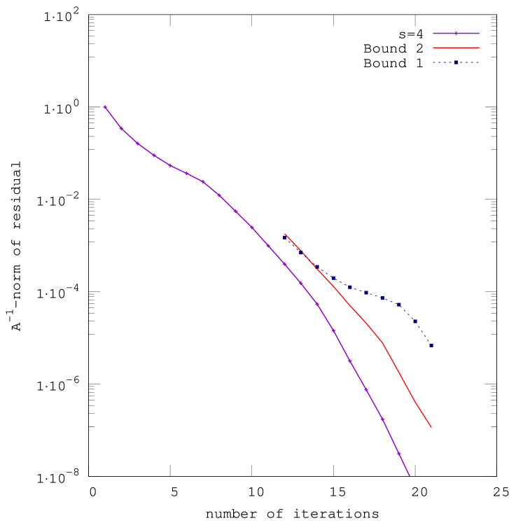
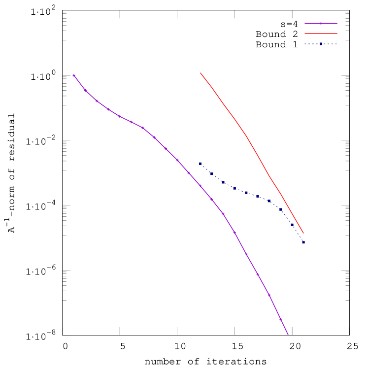
We present a series of numerical experiments illustrating the quality of both the subspace-based bounds (1) and the spectral-based bounds (24), and we compare them. We discuss different cases, namely different eigenvalue distributions of the coefficient matrix $A$, as well as taking different dimensions of the invariant subspaces in the comparison process. We also consider the effect of taking increasing numbers of right hand sides.

Without loss of generality, we consider diagonal matrices in our first five examples. In Example 4.6 we consider a preconditioned model problem. Recall that the coefficient $\alpha_{m,k_{1},k_{2}}$ in (24) depends on $k_{1}$ eigenvalues in the lower part of the spectrum, and $k_{2}$ eigenvalues in the upper part of the spectrum. Different cases of $k_{1}$ and $k_{2}$ are considered, both when the eigenvalues are simple, and when they have multiplicity $\kappa>1$. Recall also that in the bound (1) we have an invariant subpace whose basis are the columns of the matrix $Y$. In our experiments, these columns are $y_{i}=Az_{i}$, $z_{i}\in\mathbb{K}_{m}(A,{\bf R}_{0})$, and $z_{i}$ are taken to be Ritz vectors.

For each example, two sets of complementary results are presented. In one set, we follow the evolution of the Ritz values as they converge to the corresponding eigenvalues, and look at the behaviour of the two constants used in our bounds, $\alpha_{m,k_{1},k_{2}}$ in (24) and $\gamma_{m}$ in (1). In this case, we use the bounds (24) and (1) for $j=0$ as $m$ increases. We can observe than when the Ritz values are close enough to the eigenvalues, or when $\gamma_{m}$ is small enough, the convergence curve changes slope; though this point is hard to pinpoit exactly. The second set of experiments show that the bounds obtained follow closely the slope of the convergence curves, especially after the change of slope, sometimes called the onset of superlinearity, has taken hold.

Example 4.1.

Our first example is for the case $s=1$, and thus, the block method reduces to the standard case, and our bounds reduce to that presented in [29]. We consider $k_{1}=1$, $k_{2}=0$, that is, only one Ritz value (and one Ritz vector), at the lowest part of the spectrum. We do so as to examine three situations in which the Ritz value $\theta_{1}^{(m)}$ is either very close to the first eigenvalue $\lambda_{1}$ (Case 4.1.a), $\theta_{1}^{(m)}$ is between $\lambda_{1}$ and $\lambda_{2}$ (Case 4.1.b), or $\theta^{(m)}_{1}>\lambda_{2}$ (Case 4.1.c), as was done in [30]. We thus study a $100\times 100$ diagonal matrix with eigenvalues $0.1$, $0.2$, $0.3$, $0.4$, $5$, $\ldots$ , $100$. The right-hand side is a vector with all unit entries, the initial approximation ${\bf X}_{0}=x_{0}$ is the zero vector, and the initial residual is ${\bf R}_{0}=b$; i.e., the residual has equal components in all eigenvectors that form an eigenbasis so that no one eigendirection is favored.

Recall that in the expressions (1) and (31), ${\bf R}_{m+j}$ is the block CG residual at the $(m+j)$th step, and $\bar{\bf R}_{j}$ is the residual after $j$ steps of block CG applied to $\bar{\bf R}_{0}=(I-\Pi_{Q}){\bf R}_{m}$. The counter $m$ specifies the status of iteration advance of block CG when the bound starts to be employed. Hence, in the first set of experiments, as $m$ increases, $\theta_{1}$ convergences towards $\lambda_{1}$, as shown, e.g., in Table 1 below, and for fixed $m$, as $j$ increases, we look at the behavior of the bounds, as shown, e.g., in Table 2.

Case 4.1.a. The first Ritz value $\theta_{1}$ is very close to $\lambda_{1}$. Our first set of experiments are reported in Table 1, where we show the behavior of $\alpha_{m,1,0}$ and $\gamma_{m}$ at each iteration $m$. Bounds (1) and (24) are computed with $j=0$ and are presented for several values of $m$. In other words, the bounds reduced to

$$b_{1}:=\|\bar{\bf R}_{0}\|_{A^{-1}}+\gamma_{m}\|\Pi_{Q}{\bf R}_{m}\|_{A^{-1}},\mbox{ ~{}and ~{} }b_{2}:={\alpha}_{m,1,0}\|\bar{\bf R}_{0}\|_{A^{-1}}.$$ (34)

The comparison residual at iteration $m$ is $\bar{\bf R}_{0}=\|(I-\Pi_{Q}){\bf R}_{m}\|_{A^{-1}}$. Observe that despite of the fact that the convergence of the Ritz vectors is slow and non-monotone [18], which has influence on $\gamma_{m}$, the subspace bound $b_{1}$ gives sharper estimates than the spectral bound $b_{2}$; see Table 1.

Table 1: Case 4.1.a. The first Ritz value $\theta^{(m)}_{1}$ is very close to smallest eigenvalue $\lambda_{1}$. Parameters $k_{1}=1$, $k_{2}=0$, $s=1$ and $j=0$. Factors $\gamma_{m}$ and ${\alpha}_{m,1,0}$ are computed using (20) and (24), respectively. The subspace bound $b_{1}$ and the spectral bound $b_{2}$ correspond to (34).

$m$	$\theta_{1}$	$\theta_{1}/\lambda_{1}$	$\gamma_{m}$	${\alpha}_{m,1,0}$	$b_{1}$	$b_{2}$	$\|\bar{\bf R}_{0}\|_{A^{-1}}$	$\|{\bf R}_{m}\|_{A^{-1}}$
$30$	0.12659	1.26597	0.61127	1.72469	0.77367	0.92530	0.53650	0.66210
$31$	0.12280	1.22800	0.56286	1.59067	0.67380	0.79217	0.49801	0.58784
$32$	0.11708	1.17082	0.48434	1.41203	0.53402	0.60523	0.42862	0.48069
$33$	0.11138	1.11386	0.39936	1.25698	0.39652	0.42922	0.34147	0.36825
$34$	0.10771	1.07712	0.33933	1.16715	0.29890	0.31279	0.26799	0.28305

Observe that as $m$ increases, then ${\alpha}_{m,1,0}$ decreases (ideally it tends to one) and $\gamma_{m}$ also decreases (ideally tends to zero). Recall that when ${\alpha}_{m,1,0}=1$ and $\gamma_{m}=0$, then both bounds coincide. However, also note that the spectral bound $b_{2}$ is more sensitive to changes ${\alpha}_{m,1,0}$ than the bound $b_{1}$ to changes in $\gamma_{m}$. This means that $\gamma_{m}$ does not need to be close to zero in order for the subspace bound $b_{2}$ obtain a better approximation than the spectral bound $b_{1}$.

Table 2: Case 4.1.a. The first Ritz value $\theta_{1}$ very close to smallest eigenvalue $\lambda_{1}$. Parameters are $k_{1}=1$, $k_{2}=0$, $s=1$, and iteration $m=33$. Factors ${\alpha}_{m,k_{1},k_{2}}={\alpha}_{33,1,0}$ and $\gamma_{m}=\gamma_{33}$ are computed using (24) and (20), respectively. The subspace bound $b_{1,j}$ and the spectral bound $b_{2,j}$ are given by (35).

	$\theta_{1}$	${\alpha}_{33,1,0}$	$\gamma_{33}$	$\|{\bf R}_{33}\|_{A^{-1}}$
	0.11138	1.25698	0.39936	0.36825
$j$	$b_{1,j}$	$b_{2,j}$	$\|\bar{\bf R}_{j}\|_{A^{-1}}$	$\|{\bf R}_{33+j}\|_{A^{-1}}$
$1$	0.34058	0.35903	0.28563	0.28305
$2$	0.29627	0.30365	0.24157	0.23350
$3$	0.27034	0.27142	0.21594	0.20939
$4$	0.25733	0.25542	0.20321	0.19836
$5$	0.25064	0.24739	0.19684	0.19279
$6$	0.24635	0.24246	0.19293	0.18896
$7$	0.24228	0.23803	0.18944	0.18476
$8$	0.23651	0.2320	0.18474	0.17775
$9$	0.22602	0.22135	0.17654	0.16362
$10$	0.20638	0.20139	0.16165	0.13714

In the second set of experiments, we examine our two bounds in the same stage of convergence of the Ritz values to their corresponding eigenvalues. To this end, we fix $m=33$ and take iterations $j$ from $j=1$ to $j=10$. For easier reading we denote our bounds as follows,

$$\left\{\begin{array}[]{ccl}b_{1,j}&=&\min_{{\bf D}\in A\mathbb{K}_{j}(A,{\bf R}_{m})}\left\{\|(I-\Pi_{Q})({\bf R}_{m}-{\bf D})\|_{A^{-1}}\right.\vspace{0.07in}\\ &&\qquad\qquad\qquad\qquad\qquad\left.+\gamma_{m}\|\Pi_{Q}({\bf R}_{m}-{\bf D})\|_{A^{-1}}\right\}\qquad\mbox{ and }\vspace{0.1in}\\ b_{2,j}&=&\alpha_{m,k_{1},k_{2}}\|\bar{\bf R}_{j}\|_{A^{-1}}.\end{array}\right.$$ (35)

Table 2 shows the behavior of expressions the subspace bound $b_{1,j}$ and the spectral bound $b_{2,j}$ Note that for this example, both bounds behave similarly.

Case 4.1.b. The Ritz value $\theta_{1}$ is between $\lambda_{1}$ and $\lambda_{2}$. The first set of experiments, for $m=21,\ldots,25$, are presented in Table 3. In this interval, the factor ${\alpha}_{m,1,0}$ varies considerable with $m$. This is in contrast with $\gamma_{m}$ which does not vary as much.. The variation of ${\alpha}_{m,1,0}$ is due to the proximity of $\theta^{(m)}_{1}$ to $\lambda_{2}$, which yields a very rough estimate by the spectral bound $b_{2}$ of the block CG behavior. The estimate is improved either once $\theta^{(m)}_{1}$ moves away from $\lambda_{2}$ or by replacing the factor $\alpha_{m}$ by $\theta^{(m)}_{1}/\lambda_{1}$ as suggested in [28]. The latter results in a bound ($\frac{\theta_{1}}{\lambda_{1}}\|\bar{\bf R}_{0}\|_{A^{-1}}$) which is sharper than either of our bounds in this case.

Table 3: Case 4.1.b. Ritz value $\theta_{1}$ in $\left[\lambda_{1},\lambda_{2}\right]$. Parameters $k_{1}=1$, $k_{2}=0$, $s=1$, and $j=0$. Factors ${\alpha}_{m,1,0}$ and $\gamma_{m}$ are computed using (24) and (20), respectively. The subspace bound $b_{1}$ and the spectral bound $b_{2}$ correspond to (34).

$m$	$\theta^{(m)}_{1}$	$\theta_{1}/\lambda_{1}$	$\gamma_{m}$	${\alpha}_{m,1,0}$	$b_{1}$	$b_{2}$	$\|\bar{\bf R}_{0}\|_{A^{-1}}$	$\|{\bf R}_{m}\|_{A^{-1}}$
21	0.20181	2.0181	0.86898	110.93237	2.11922	113.62360	1.02426	1.62383
22	0.17786	1.7786	0.80929	8.0359	1.78204	6.28417	0.964314	1.39672
23	0.15595	1.5595	0.74794	3.5404	1.43954	2.47657	0.85200	1.15887
24	0.14271	1.4271	0.70553	2.4913	1.18655	1.59363	0.73686	0.97427
25	0.13622	1.3622	0.68186	2.1359	1.03745	1.29275	0.65704	0.86194

Table 4: Case 4.1.b. Residual bounds at $m=23$, when $\theta_{1}$ is in the middle of $\left[\lambda_{1},\lambda_{2}\right]$. Parameters $k_{1}=1$, $k_{2}=0$ and $s=1$. Factors ${\alpha}_{23,1,0}$ corresponds to (24) and $\gamma_{m}$ to (20). The subspace bound $b_{1,j}$ and the spectral bound $b_{2,j}$ correspond to (35).

	$\theta_{1}$	$\alpha_{23,1,0}$	$\gamma_{23}$	$\|{\bf R}_{23}\|_{A^{-1}}$
	0.15595	3.54044	0.74794	1.15887
$j$	$b_{1,j}$	$b_{2,j}$	$\|\bar{\bf R}_{j}\|_{A^{-1}}$	$\|{\bf R}_{23+j}\|_{A^{-1}}$
$1$	1.28592	2.47657	0.69950	0.97427
$2$	1.15295	2.01543	0.56925	0.86194
$3$	1.06385	1.71144	0.48339	0.80285
$4$	1.01284	1.54247	0.43567	0.77255
$5$	0.98455	1.45406	0.41070	0.75507
$6$	0.96687	1.40444	0.39668	0.74175
$7$	0.95238	1.36986	0.38691	0.72694
$8$	0.93562	1.33628	0.37743	0.70399
$9$	0.90988	1.29108	0.36466	0.66210
$10$	0.86496	1.21714	0.34378	0.58784

Fig. 1: Example 4.1.c. Behavior of the factors ${\alpha}_{m,1,0}$ and $\gamma_{m}$ of our bounds given in (34) for each $m$, the number of iterations. The smallest Ritz value $\theta^{(m)}_{1}$ at the $m$th iteration and smallest eigenvalue $\lambda_{1}$ of the matrix $A$.

For the second set of experiments, we consider $m=23$, when $\theta^{(m)}_{1}$ fall almost exactly in the middle of $\left[\lambda_{1},\lambda_{2}\right]$. Hence, the factor ${\alpha}_{m,1,0}$ is large and the spectral bound $b_{2,j}$ overestimates the residual norm, as shown in Table 4. Note that for this case, the subspace bound $b_{1,j}$ is sharper than the spectral bound $b_{2,j}$ for all $j$.

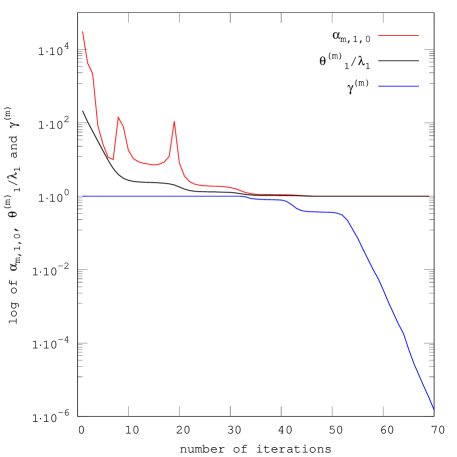
Case 4.1.c. When $\theta^{(m)}_{1}$ is outside the interval $[\lambda_{1},\lambda_{2}]$. This occurs when $m\leq 20$. The factors ${\alpha}_{m,1,0}$ and $\gamma_{m}$ have very different behavior as reported in Figure 1. Observe that ${\alpha}_{m,1,0}$ has large variations when $\theta^{(m)}_{1}$ approaches a wrong eigenvalue, and consequently the spectral bound computed with these factors do not provide any useful information. On the other hand, for $m\leq 20$ the value of $\gamma_{m}$ remains almost equal to $1$, that means that the subspace bound $b_{1,j}$ in (35) can be computed as $\|(I-\Pi_{Q})\bar{\bf R}_{j}\|_{A^{-1}}+\|\Pi_{Q}\bar{\bf R}_{j}\|_{A^{-1}}$.

In summary, Example 4.1 illustrates the behavior of the bounds in several stages of the convergence of the Ritz value $\theta^{(m)}_{1}$ towards the eigenvalue $\lambda_{1}$. In Case 4.1.a, both bounds behave similarly when the Ritz value has sufficiently converged to its corresponding eigenvalue. In the other two cases, the subspace bound is better than the spectral bound when the Ritz value $\theta^{(m)}_{1}$ is far away of the corresponding eigenvalue $\lambda_{1}$.

Example 4.2.

Here, we consider the four smallest eigenvalues in the construction of the bounds, i.e., $k_{1}=4$ and $k_{2}=0$. In this experiment, the matrix $A$ and the initial iterate ${\bf X}_{0}$ are the same as in Example 4.1.

In the first set of experiments, we present in Table 5, the convergence of the Ritz values $\theta_{i}^{(m)}$, $i=1,\ldots,4$, to the four lowest eigenvalues, and the behavior of ${\alpha}_{m,k_{1},k_{2}}={\alpha}_{m,4,0}$ and $\gamma_{m}$. In addition, we present the subspace bound $b_{1}$ and the spectral bound $b_{2}$ given in (34), and the norms of the comparison residual $\bar{\bf R}_{0}$ and the block CG residual ${\bf R}_{m}$. Note that since $\theta^{(m)}_{4}$ is close to an eigenvalue different than $\lambda_{4}$, namely $\lambda_{5}$, the factor ${\alpha}_{m,4,0}$ varies widely.

Table 5: Example 4.2. Ritz values $\theta_{i}^{(m)}$, $i=1,\cdots,4$. The bounds area computed with $j=0$, and parameters $k_{1}=4$ and $k_{2}=0$. Factors ${\alpha}_{m,4,0}$ corresponds to (32) and $\gamma_{m}$ to (20). The subspace bound $b_{1}$ and the spectral bound $b_{2}$ correspond to (34). The four smallest eigenvalues are $\lambda_{1}=0.1,\lambda=0.2,\lambda=0.3$ and $\lambda=0.4$.

$m$	$\theta^{(m)}_{1}$	$\theta^{(m)}_{2}$	$\theta^{(m)}_{3}$	$\theta^{(m)}_{4}$	$\alpha_{m,4,0}$	$\gamma_{m}$	$b_{1}$	$b_{2}$	$\|\bar{\bf R}_{0}\|_{A^{-1}}$	$\|{\bf R}_{m}\|_{A^{-1}}$
39	0.10485	0.24301	0.39061	5.00336	29249.6	0.99998	0.23883	1340.984	0.04584	0.19836
40	0.10469	0.24235	0.39033	4.99812	52236.3	0.99996	0.22012	1547.637	0.02962	0.19279
41	0.10458	0.24189	0.39013	4.98636	7124.5	0.99983	0.21305	184.532	0.02590	0.18896
42	0.10446	0.24138	0.38991	4.35890	131.885	0.98594	0.21336	4.53408	0.03437	0.18476
43	0.10426	0.24049	0.38949	2.33890	16.9294	0.95700	0.21476	0.88256	0.05213	0.17775
44	0.10384	0.23842	0.38838	1.10663	5.3865	0.88939	0.20429	0.40350	0.07491	0.16362
45	0.10302	0.23329	0.38414	0.58421	2.40210	0.75256	0.16799	0.16799	0.09033	0.13714
46	0.10185	0.22274	0.35799	0.42276	1.46327	0.55404	0.11397	0.12184	0.08327	0.10002

Fig. 2: Example 4.2. Block CG residual $\|{\bf R}_{m}\|_{A^{-1}}$, subspace bound 1 and spectral bound 2 from (35) computed with $m=45$ and $m=50$. Parameters $k_{1}=4$ and $k_{2}=0$.

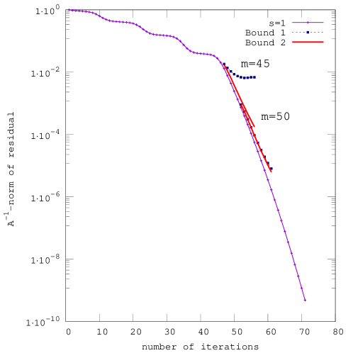
The second set of experiments are presented in Figure 2, where we see the behavior of the residual norm $\|{\bf R}_{m}\|_{A^{-1}}$ of the block CG, the subspace bound $b_{1,j}$ and spectral bound $b_{2,j}$ as expressed in (35). Note that at iteration $m=45$ the spectral bound $b_{2,j}$ is sharper than the subspace bound $b_{1,j}$. This is because the subspace bound $b_{1,j}$ with a moderate $\gamma_{m}$ ($\gamma_{m}=0.75256$) amplifies significantly the residual component on the selected eigenspace $\mathbb{R}(Q)$. At iteration $m=50$ the selected Ritz values are very close to its respective eigenvalues and the resulting bounds are almost the same.

Fig. 3: Example 4.3. Residual convergence behavior for the block CG $\left\lVert{\bf R}_{m+j}\right\rVert_{A^{-1}}$ for $s=1,4,8$, subspace and spectral bounds $b_{1,j}$ and $b_{2,j}$ correspond to expressions (35). Parameters $k_{1}=1$ and $k_{2}=0$. Note: $m=43$ correspond to ($\alpha=1.0254$, $\gamma=0.1572$), $m=31$ correspond to ($\alpha=1.201$, $\gamma=0.4083$), and $m=27$ correspond to ($\alpha=1.0758$, $\gamma=0.2648$).

Example 4.3.

This example is designed to analyze the effect of the block size $s$ on the bounds and on the convergence of the block CG in the presence of a single eigenvalue near the origin, i.e., $k_{1}=1$ and $k_{2}=0$. This experiment considers a diagonal matrix of dimension $404\times 404$ with eigenvalues on the diagonal with values $0.0005,0.08,\ldots,2.42$, that is, the matrix has one isolated eigenvalue near to zero and the other $403$ eigenvalues are equally distributed between $0.08$ and $2.42$. It is expected to observe superlinear convergence once the method captures the lowest eigenvalue $0.005$.

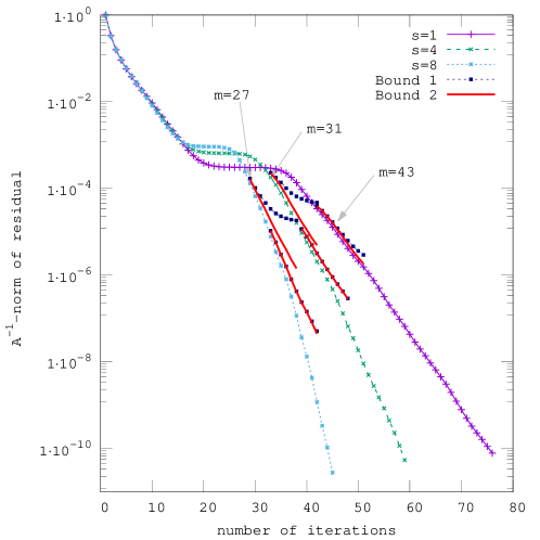
Figure 3 shows the convergence history for block sizes $s=1$, $4$ and $8$. In this example, and in those in the rest of the section, when $s>1$, the matrix ${\mathbf{B}}$ has repeated copies of $b$, but the initial set of vectors in ${\mathbf{X}}_{0}$ are nonzero and randomly generated, implying that ${\mathbf{R}}_{0}$ has all distinct columns. On each residual history, we plot the subspace bound $b_{1,j}$ and the spectral bound $b_{2,j}$ at two different stages of convergence: soon after the onset of superlinearity occurs, and a numbero of iterations later. Observe that for values of $m$ relatively large, both bounds capture well the slope of the superlinear regime. In addition, observe that as the block size is increased, block CG hastens the onset of superlinear convergence, but going from $s=4$ to $s=8$ the difference in the onset is moderate.

(a) Behavior of $\alpha_{m,1,0}$

(b) Behavior of $\gamma_{m}$

Fig. 4: Example 4.3. Behavior of $\alpha_{m,1,0}$ and $\gamma_{m}$ correspond to the number of iterations $m$. $\alpha_{m,1,0}$ is computed with expression (32) and $\gamma_{m}$ is computed with expression (20). Parameters $k_{1}=1$, $k_{2}=0$ and $s=1,4,8$.

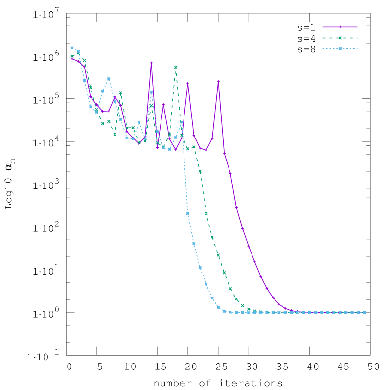
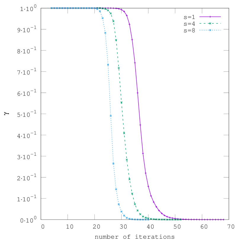
Observe also that near the onset of superlinearity (for earlier $m$) the spectral bound $b_{2,j}$ is sharper than subspace bound $b_{1,j}$. This is due to the fact that factor $\gamma_{m}$ has moderate values ($\gamma_{m}\in[0.5,1]$)), introducing in the subspace bound $b_{1,j}$ a contribution from the invariant subspace $\mathbb{R}(Q)$. It is important to remark that moderate values of $\gamma_{m}$ are in connection with the rate of convergence of Ritz vectors, which is smaller than that of the convergence of the Ritz values. This can be appreciated by comparing Figures 4(a) and 4(b), that the convergence of $\alpha_{m,1,0}$ (to one) is faster than the convergence of $\gamma_{m}$ (to zero).

In addition, in Figure 4(a), it can be observed the erratic convergence behavior of $\alpha_{m,1,0}$. In fact, it takes large oscillatory values before approaching the final interval of convergence of the Ritz values. On the other hand, the behavior of $\gamma_{m}$ is smooth and well behaved; see Figure 4(b). This indicates that the subspace bound $b_{1,j}$ is less sensitive to the stage of convergence of the Ritz value, hence it can be used safely to describe the behavior in this region.

Example 4.4.

The objective of this example is to analyze the effect of the block size $s$ on the convergence of block CG and the behavior of the bounds to capture the superlinearity in presence of a cluster of eigenvalues near the origin. To this end, we consider a diagonal matrix of dimension $404\times 404$ with eigenvalues on the diagonal with values $0.0005$, $0.0015$, $0.0025$, $0.0035$, $0.0045$, $0.0055$, $0.08,\ldots,2.42$. The matrix has six clustered eigenvalues near zero and the rest distributed uniformly between $0.08$ and $2.42$.

Fig. 5: Example 4.4. Residual convergence behavior for the block CG $\left\lVert{\bf R}_{m+j}\right\rVert_{A^{-1}}$ for $s=1,2,4,8$, The subspace bound $b_{1,j}$ and the spectral bound $b_{2,j}$ are given by (35). The parameters are $k_{1}=6$ and $k_{2}=0$. Note: $m=29$ correspond to ($\alpha=1.080$, $\gamma=0.2702$), $m=43$ correspond to ($\alpha=1.1630$, $\gamma=0.3674$), $m=63$ correspond to ($\alpha=1.1072$, $\gamma=0.3097$) and $m=103$ correspond to ($\alpha=1.2057$, $\gamma=0.4102$).

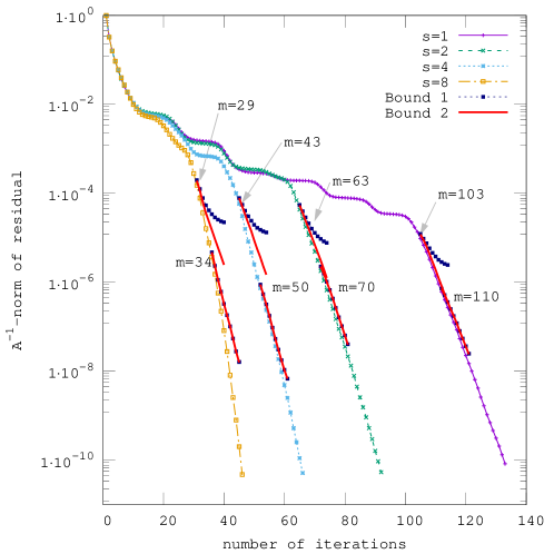
Figure 5 shows the convergence history of block CG, considering the invariant subspace associated to the six lowest eigenvalues, i.e., both bounds are computed using $k_{1}=6$ and $k_{2}=0$ for each block size ($s=1$, $2$, $4$ and $8$). Our observations here are very similar to those in the previous example, where a single eigenvalue was considered. In particular, note that that when the block size is increased, the superlinear behavior starts earlier. This shows the dependency of the onset of the superlinear behavior on the block size. Moreover, as in the previous example, this example suggests that block CG (with $s>1$) hastens the onset of the superlinearity in the presence of clustered eigenvalues.

(a) $k_{1}=1$, $k_{2}=0$ and $s=1$.

(b) $k_{1}=2$ , $k_{2}=0$ and $s=1$.

(c) $k_{1}=4$, $k_{2}=0$ and $s=4$.

(d) $k_{1}=5$, $k_{2}=0$ and $s=4$.

Fig. 6: Example 4.5. Residual convergence behavior for block CG. The subspace bound $b_{1,j}$ and the spectral bound $b_{2,j}$ are given by (35). (a) Parameters values $s=k_{1}$ and $\alpha_{80,1,0}=1.00002$ and $s=1$, (b) Parameters values $k_{1}=2$ and $\alpha_{80,2,0}=1.83221\times 10^{8}$ and $s=1$,, (c) Parameters values $s=k_{1}$ and $\alpha_{50,4,0}=1.00108$ and $s=4$, and (d) Parameters values $k_{1}=5$ and $\alpha_{50,5,0}=4.718055\times 10^{9}$ and $s=4$.

Example 4.5.

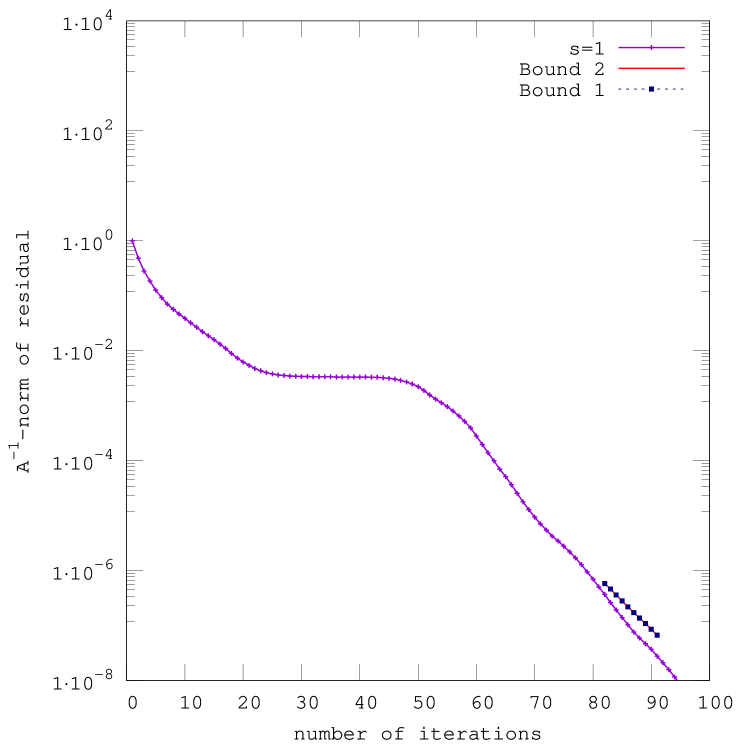
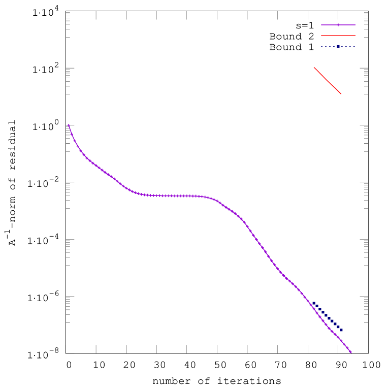
In this example we analyze effect of an eigenvalue with algebraic multiplicity $\kappa>1$ on the two bounds we study. To this end, we consider a $384\times 384$ matrix with an eigenvalue $\lambda=0.0005$ with algebraic multiplicity $5$ in the lowest part of its spectrum. The rest of eigenvalues are uniformly distributed between $0.065$ and $5.42$.

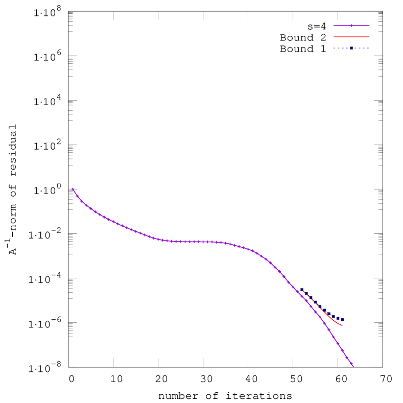
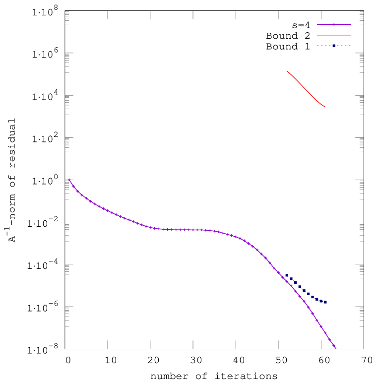
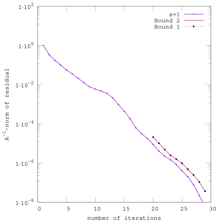
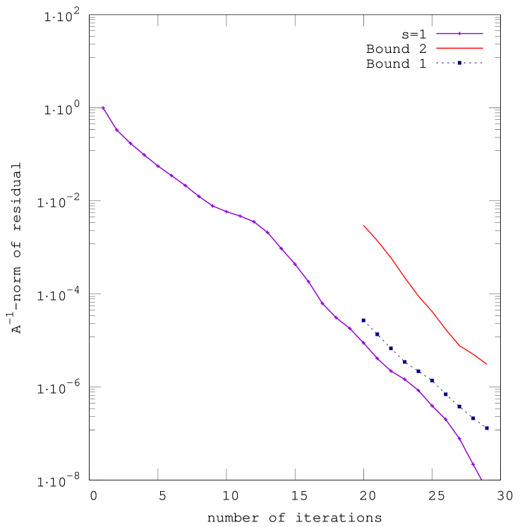
Figure 6 shows the block CG residual, the subspace bound $b_{1,j}$, and the residual bound $b_{2,j}$. When the parameter $k_{1}=s$, the block size (see Figures 6(a) and 6(c)), the spectral bound $b_{2,j}$ (defined in (35) with $\alpha_{m,k_{1},k_{2}}$ approximates adequately the behavior of the residual. On the other hand, if $k_{1}>s$ (see Figures 6(b) and 6(d)), then the bound captures the slope but it is far from sharp. In all cases the subspace bound $b_{1,j}$ approximates adequately the behavior of the residual.

At this point, it is important to remark that the CG polynomial only captures one copy of the eigenvalue with multiplicity, but block CG can find up to $s$ copies in the case of repeated eigenvalues [27]. This remark also applies for clustered eigenvalues. Hence, if $s=k_{1}\leq\kappa$, block CG captures $s$ eigenvalues and the spectral bound $b_{2,j}$ which uses these $k_{1}=s$ eigenvalues approximates well the residual. However, if $s<k_{1}\leq\kappa$, then the bound is expected to capture more eigenvalues than the block CG is able to capture, and consequently the approximation bound is not sharp. Note the different horizontal scales in Figures 6(c) and (d) for $s=4$, compared to that in Figures 6(a) and (b) for $s=1$.

The analysis of this example suggest that when an eigenvalue with algebraic multiplicity $\kappa$ is considered, the spectral-based bound approximates adequately the residual behavior when the number of eigenvalues taken as reference (denoted by $k_{1}\leq\kappa$) is at most equal to the block size $s$.

In this example, it can also be observed that as the block size $s$ is increased, the number of eigenvalues captured by block CG is larger, hence the onset of the superlinear convergence occurs earlier (compare for instance Figures 6(b) and 6(d). This is in accordance with the observation made in Example 4.4 showing a close relationship between block size $s$ and the onset of superlinear convergence.

(a) $k_{1}=1$, $k_{2}=0$ and $s=1$.

(b) $k_{1}=2$, $k_{2}=0$ and $s=1$ .

(c) $k_{1}=4$, $k_{2}=0$ and $s=4$.

(d) $k_{1}=5$, $k_{2}=0$ and $s=4$ .

Fig. 7: Example 4.6. Poisson matrix preconditioned using an incomplete Cholesky factorization. Residual convergence behavior for the block CG, the bound $b_{2,j}$ corresponding to expression (35) and $\left\lVert\bar{\bf R}_{j}\right\rVert_{A^{-1}}$. (a) Parameters $k_{1}=1$ and $\alpha_{20,1,0}=1.01$. (b) Parameters $k_{1}=2$ and $\alpha_{20,2,0}=89.4478$. (c) Parameters $k_{1}=4$ and $\alpha_{10,4,0}=1.448558$. (d) Parameters $k_{1}=7$ and $\alpha_{10,7,0}=29.224$.

Example 4.6.

For our last example we consider a $400\times 400$ matrix obtained with a standard discretization of the 2D Poisson equation, presonditioned with incomplete Cholesky factorization with no fill. Thus, the coefficient matrix is $\tilde{A}=L^{-1}AL^{-T}$. The maximum eigenvalue is 1.2015 and the minimum is 0.0724. The ten smallest eigenvalues are $0.0724$, $0.1652$, $0.1699$, $0.2483$, $0.2971$, $0.2994$, $0.3486$, $0.3742$, $0.4362$, $0.4367$, $0.4396$, $0.4802$. The rest of the eigenvalues are distributed between $0.5014$ and $1.2015$.

Figure 7 shows the behavior of the residual, together with the subspace and spectral bounds $b_{1,j}$ and $b_{2,j}$ as in (35). In one set of experiments, we consider the block size $s=1$, and parameters $k_{1}=1$ and $k_{2}=0$, and $k_{1}=2$ and $k_{2}=0$. Figure 7(a) shows a good approximation of the bounds to the block CG residual. This is in accordance with the observation made that the convergence is mainly due to the convergence of the first eigenvalue. It can also be observed (similar to Example 4.5) that when $k_{1}$ is larger than $s$, the bounds capture the slope of the residual but the spectral bound $b_{2,j}$ is far from sharp (see Figure 7(b)). Similar observation can be done for a larger block sizes, for instance, Figures 7(c) and 7(d) for values of $k_{1}=4$, $k_{2}=0$ and $s=4$, and $k_{1}=5$, $k_{2}=0$ and $s=5$, respectively.

Finally, comparing Figures 7(c) and 7(d), since more eigenvalues are captured when the block size is increased, the onset of the superlinear convergence occurs earlier. Again, note the different horizontal scale of these two figures for $s=4$ as compared to those with $s=1$.

5 Conclusions

We extended the a posteriori spectral bound introduced by van der Sluis and van der Vorst [28] to the block CG case. We have also implemented the subspace bound introduced by Simoncini and Szyld [21]. Numerical experiments show that both bounds capture the slope of the residual after the onset of superlinearity. In addition, when there is a cluster of eigenvalues in the lower part of the matrix spectrum, the spectral bound captures better the superlinearity even at the near the onset of superlinearity, while the subspace bound is sharper in presence of repeated eigenvalues.

Analyzing the bounds and the residual behavior of the block CG method, it can be observed that the block method accelerates the convergence because it captures more eigenvalues. Therefore, in the presence of a cluster or repeated eigenvalues in the lower part of the spectrum, the larger the block size $s$, the earlier is the onset of the superlinear convergence. Hence in these cases we suggest the use of block CG with the block size of the order of to the size of the cluster.

References

- [1] O. Axelsson and J. Karátson, On the rate of convergence of the conjugate gradient method for linear operators in hilbert space, Numerical Functional Analysis and Optimization, 23 (2002), pp. 285–302.
- [2] B. Beckermann and A. B. Kuijlaars, Superlinear CG convergence for special right-hand sides, Electronic Transactions on Numerical Analysis, 14 (2002), pp. 1–19.
- [3] S. L. Campbell, I. C. F. Ipsen, C. T. Kelley, and C. D. Meyer, GMRES and the minimal polynomial, BIT Numerical Mathematics, 36 (1996), pp. 664–675.
- [4] A. El Guennouni, K. Jbilou, and H. Sadok, The block Lanczos method for linear systems with multiple right-hand sides, Applied Numerical Mathematics, 51 (2004), pp. 243 – 256.
- [5] H. C. Elman, D. J. Silvester, A., and A. J. Wathen, Performance and analysis of saddle point preconditioners for the discrete steady-state navier-stokes equations, Numer. Math, 90 (2000), pp. 665–688.
- [6] A. Frommer, K. Lund, and D. B. Szyld, Block Krylov subspace methods for functions of matrices, Electronic Transactions on Numerical Analysis, 47 (2017), pp. 100–126.
- [7] , Block Krylov subspace methods for functions of matrices II: Modified block FOM, SIAM Journal on Matrix Analysis and Applications, 41 (2020), pp. 804–837.
- [8] T. Gergelits and Z. Strakos, Composite convergence bounds based on Chebyshev polynomials and finite precision conjugate gradient computations, Numerical Algorithms, 65 (2014), p. 759?782.
- [9] G. H. Golub and C. F. Van Loan, Matrix Computations, The Johns Hopkins University Press, Baltimore, 4th ed., 2013.
- [10] A. Greenbaum, Iterative methods for solving linear systems, SIAM, Philadelphia, 1997.
- [11] M. H. Gutknecht, Block Krylov space methods for linear systems with multiple right-hand sides: An introduction, in Modern Mathematical Models, Methods and Algorithms for Real World Systems, Abul Hasan Siddiqi, Iain Duff, and Ole Christensen, eds., Anamaya, New Delhi, 2007, pp. 420–447.
- [12] M. H. Gutknecht and T. Schmelzer, The block grade of a block Krylov space, Linear Algebra and its Applications, 430 (2009), pp. 174 – 185.
- [13] M. R. Hestenes and E. Stiefel, Methods of conjugate gradients for solving linear systems, Journal of Research of the National Bureau of Standards, 49 (1952).
- [14] T. Kato, Perturbation theory for linear operators, Springer, Berlin, 2013.
- [15] M. D. Kent, Chebyshev, Krylov, Lanczos: Matrix Relationship and Computations, PhD thesis, Department of Computer Science - Stanford University, 1989.
- [16] M. Kubínová and K. M. Soodhalter, Admissible and attainable convergence behavior of block arnoldi and gmres, SIAM Journl on Matrix Analysis and Applications, 41 (2020), pp. 464–486.
- [17] D. P. O’Leary, The block conjugate gradient algorithm and related methods, Linear Algebra and its Applications, 29 (1980), pp. 293–322.
- [18] Y. Saad, On the Rates of Convergence of the Lanczos and the Block-Lanczos Methods, SIAM Journal on Numerical Analysis, 17 (1980), pp. 687–706.
- [19] Y. Saad, Iterative methods for sparse linear systems, vol. 82, SIAM, Philadelphia, 2003.
- [20] V. Simoncini, Ritz and Pseudo-Ritz values using matrix polynomials, Linear Algebra and its Applications, 241 (1996), pp. 787 – 801.
- [21] V. Simoncini and D. B. Szyld, On the occurrence of superlinear convergence of exact and inexact Krylov subspace methods, SIAM Review, 47 (2005), pp. 247–272.
- [22] , Recent computational developments in Krylov subspace methods for linear systems, Numerical Linear Algebra with Applications, 14 (2007), pp. 1–59.
- [23] , On the superlinear convergence of MINRES, in Numerical Mathematics and Advanced Applications 2011 - Proceedings of ENUMATH 2011, the 9th European Conference on Numerical Mathematics and Advanced Applications, Leicester, September 2011, Berlin and Heidelberg, 2013, Springer, pp. 733–740.
- [24] G.L.G. Sleijpen and A. van der Sluis, Further results on the convergence behavior of conjugate-gradients and Ritz values, Linear Algebra and its Applications, 246 (1996), pp. 233 – 278.
- [25] G. W. Stewart and J.-G. Sun, Matrix Perturbation Theory, Academic Press, London, 1990.
- [26] Z. Strakos, On the real convergence rate of the conjugate gradient method, Linear Algebra and its Applications, 154-156 (1991), pp. 535–549.
- [27] R. Underwood, An iterative block Lanczos method for the solution of large sparse symmetric eigenproblems, PhD thesis, Department of Computer Science, Tech Rept. 496, Stanford University, 1975.
- [28] A. van der Sluis and H. A. van der Vorst, The rate of convergence of Conjugate Gradients, Numerische Mathematik, 48 (1986), pp. 543–560.
- [29] A. van der Sluis and Henk A. van der Vorst, The convergence behavior of Ritz values in the presence of close eigenvalues, Linear Algebra and its Applications, 88 (1987), pp. 651–694.
- [30] H. A. van der Vorst and C. Vuik, The superlinear convergence behaviour of GMRES, Journal of Computational and Applied Mathematics, 48 (1993), pp. 327 – 341.
- [31] R. Winther, Some superlinear convergence results for the conjugate gradient method, SIAM Journal on Numerical Analysis, 17 (1980), pp. 14–17.