Online Graph Topology Learning from
Matrix-valued Time Series
Abstract
This paper is concerned with the statistical analysis of matrix-valued time series. These are data collected over a network of sensors (typically a set of spatial locations) along time, where a vector of features is observed per time instant per sensor. Thus each sensor is characterized by a vectorial time series. We would like to identify the dependency structure among these sensors and represent it by a graph. When there is only one feature per sensor, the vector auto-regressive models have been widely adapted to infer the structure of Granger causality. The resulting graph is referred to as causal graph. Our first contribution is then extending VAR models to matrix-variate models to serve the purpose of graph learning. Secondly, we propose two online procedures respectively in low and high dimensions, which can update quickly the estimates of coefficients when new samples arrive. In particular in high dimensional regime, a novel Lasso-type is introduced and we develop its homotopy algorithms for the online learning. We also provide an adaptive tuning procedure for the regularization parameter. Lastly, we consider that, the application of AR models onto data usually requires detrending the raw data, however, this step is forbidden in online context. Therefore, we augment the proposed AR models by incorporating trend as extra parameter, and then adapt the online algorithms to the augmented data models, which allow us to simultaneously learn the graph and trend from streaming samples. In this work, we consider primarily the periodic trend. Numerical experiments using both synthetic and real data are performed, whose results support the effectiveness of the proposed methods.
Keywords: Graph learning, matrix-variate data, auto-regressive models, homotopy algorithms.
1 Introduction
The identification of graph topology responds to increasing needs of data representation and visualization in many disciplines, such as meteorology, finance, neuroscience and social science. It is crucial to reveal the underlying relationships between data entries, even in the settings where the natural graphs are available. For example in Mei & Moura [23], a temperature graph is inferred from the multivariate time series recording temperatures of cities around the continental United States over one-year period. It differs from the distance graph, however exhibits a better performance in predicting weather trends. Many methods have been proposed to infer graphs for various data processes and application settings [28, 9]. The problem of graph learning is that, given the observations of multiple features represented by random variables or processes, we would like to build or infer the cross-feature relationship that takes the form of a graph, with the features termed as nodes. According to data nature and the type of relationship, there are two main lines of work in the graph learning domain using statistic tools.
The first line considers the features represented by random variables with iid observations. Moreover, it assumes that
| (1.1) |
The works are interested in inferring the conditional dependency structure among , which is encoded in the sparsity structure of precision matrix . The resulting models are known as Gaussian graphical models [24, 11], and the sparse estimators are called graphical lasso. There are also variants for stationary vector processes, see Bach & Jordan [1] and Songsiri & Vandenberghe [29], whereas the relationship considered is still the conditional dependence.
The second line considers scalar processes, denoted by , and the inference of Granger causality relationship among them from the observed time series. By contrast to the Gaussian assumption, this line supposes that is vector autoregressive (VAR) process222For simplicity, we omit the intercept term here by assuming the process has zero mean. The process mean will be treated properly in Section 4.
| (1.2) |
where is a white noise process with variance , and are the coefficients. The Granger causality is defined pairwise: is said to Granger cause , if can be predicted more efficiently when the knowledge of in the past and present is taken into account. More technical definition see Lütkepohl [21, Section 2.3.1]. The causal graph then refers to such a graph where each node represents a scalar process, and the edges represent Granger causality.
The advantage of VAR assumption is that the topology of causal graph is encoded in the sparsity structure of the coefficient matrices. More specifically, if the processes are generated by a stationary VAR() model, then does not cause if and only if all the -th entries of the true coefficient matrices [21, Corollary 2.2.1]. Thus, we can retrieve the graph topology from the common sparsity structure in . In low-dimensional regime, this structure can be identified through Wald test, which tests linear constraints for the coefficients.
The works in literature therefore focus on the inference of causal graphs in high-dimensional regime. The inference of the exact Granger causal graph is mainly considered in Bolstad et al. [3], Zaman et al. [36]. Bolstad et al. [3] propose to consider the group lasso penalty, , to the usual least squares problem of VAR() models, in order to infer the common sparsity structure of coefficient matrices . Zaman et al. [36] develop the online procedure for this estimation problem. Mei & Moura [23] define a variant of VAR model, where the sparse structure of coefficients does not directly equal the graph topology, but the topology of -hop neighbourhoods 333For a node, its neighbours are in the -hop neighbourhood of the node. All the neighbours of its neighbours are in the -hop neighbourhood of the node, so far and so forth.. More specifically, they suppose that , where is the adjacency matrix to infer, and is the identity matrix. Such models can thus capture the influence from more nodes. The estimation of the underlying adjacency matrix relies on the Lasso penalty to promote the sparsity.
In this paper, we continue the second line by considering random processes in graph learning. However, instead of a scalar process for each feature, we consider a vector process . We wish to learn a graph of nodes that represents the causality structure among . An example data set of this setting is given in Figure 1.
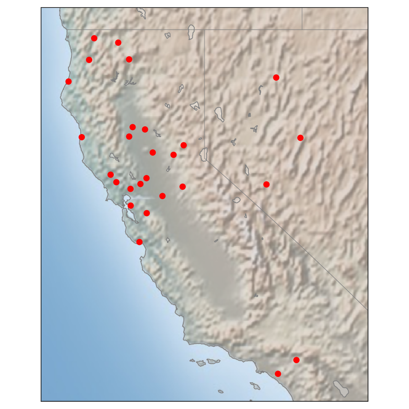
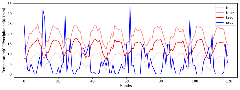
To this end, we propose to firstly extend the classical VAR model for a matrix-valued time series . Secondly, we will develop the estimation methods in both low and high dimensions. In particular, the estimation is pursued in an online fashion.
Graph learning from matrix-variate time series has not been considered previously in literature, not even in offline setting. By contrast, the Gaussian graphical models and the graphical Lassos from the first line have already extended for the matrix-variate, and more generally tensor-variate observations, , in several works [37, 19, 14, 32].
In these extended works, the authors pointed out that we may apply straightforwardly the vector models to the vectorized data , however, the resulting models will suffer from the quadratic growth of the number of edges with respect to the graph size . The samples will be soon insufficient, and the computational issues will appear. Additionally, different data dimensions will be lost after the vectorization. Therefore, to make models parsimonious yet flexible, the authors proposed to apply the vector models to the vectorized data, meanwhile impose certain structures on the parameter matrices. Such structures not only decrease the number of parameters, but also are chosen to allow matrix representations and / or interpretations of the vector models. This way of extension brings twofold benefits. On one hand, the data dimensions are kept through the matrix representations, together with model interpretability. On the other hand, the equivalent vector representations allow to apply the classical theoretical results and develop from that.
For example, Zhou [37] focused the iid observations of a random matrix and the inference of the conditional dependency structure among . To this end, the author firstly applied the classical setting (1.1) by assuming
| (1.3) |
Then a Kronecker product (KP) structure444Let be an matrix and a matrix, the Kronecker product between and , denoted by is the block matrix: When and are square matrices with , we can also define the Kronecker sum between them as: , where denote the identity matrix. is imposed on the parameter matrix:
The KP structure has reduced the number of parameters from to . It also allows a matrix representation of the model by
| (1.4) |
Note that, Equation (1.3) and Equation (1.4) are equivalent definitions. Thanks to the vector representation, the conditional dependency structure among the random variables can be easily retrieved from the sparsity structure of . In this case, the KP structure also allows an interpretation of the proposed model. Since the KP structure in an adjacency matrix corresponds to a tensor product of subgraphs, when taking as an adjacency matrix, the embedding of KP structure implies that the total conditional dependence structure is a product graph of the two sub-graphs defined respectively by and . The two sub-precision matrices and are in effect separately associated with the row and column dimensions of , which can be equivalently shown by matrix representation (1.4). To furthermore infer sparse graph structures, sparsity is supposed in and .
In addition to the KP structure, another common structure to impose is the Kronecker sum (KS). For example, Kalaitzis et al. [19] performed matrix-variate graph learning by relying on:
| (1.5) |
In this case, the KS does not allow an equivalent definition in matrix notation. However, it still gives an interpretation, similarly to the KP one. By contrast to a tensor product, the KS structure in an adjacency matrix corresponds to a Cartesian product. Thus the above model implies that the total conditional dependence structure is a Cartesian product graph of the two sub-graphs respectively for the raw and column dimensions.
Even though Models (1.5) and (1.4) are defined by the vectorized data, they take into account the row and column index of each entries . Therefore, such models should be classified as matrix models instead of vector models.
We follow the same principles to extend VAR models for matrix-variate time series . We first apply VAR models onto the vectorized data:
| (1.6) |
Secondly, we propose to impose KS structure on the coefficient matrix :
Following the relations of the KS to the matrix vectorization, we have the matrix representation of Model (1.6):
| (1.7) |
Similarly to the cited works on matrix-variate Gaussian graphical models, the vector definition (1.6) indicates that the Granger causality structure among the scalar processes still corresponds to the sparsity structure of . The KS structure furthermore implies this total causality structure is the Cartesian product of a row and a column sub-graphs, defined respectively by and . More detailed explanation of how these processes interact through the KS product will given in the next section.
Given this extended autoregressive model, the main content of this paper will thus be on the estimation of and . In particular, the estimation is pursued in an online fashion with sparsity supposed only in , which raises technical challenges in both low and high dimensions. In this context, our primary contribution is extending the homotopy algorithms of classical Lasso to a new Lasso-type problem, which is motivated by the high dimensional inference. The derived algorithms are able to update the related Lasso estimator as either i) time evolves from to ; ii) the penalization parameter is updated; or iii) both i) and ii) occur simultaneously. Additionally, an data-adaptive tuning procedure is also derived, which can tune the penalization parameter value of the Lasso problem automatically when time evolves from to . The contribution also relies on the fact that the derivations and the algorithms do not depend on our specific structure assumed in , thus can be applied to the online inference of many other parametric models under structure and sparsity assumptions.
Besides the new Lasso algorithms which are applied to the high-dimensional inference, in low-dimension, we also propose an online procedure for the estimation. Both online procedures take into account the presence of trends in time series, therefore can be applied directly on the real time series. The total of proposed methods constitute a realistic methodology to perform online graph learning matrix-variate time series, which itself is a new data type in the graph learning domain to our best knowledge. This makes a significant contribution.
Lastly, we would like to relate to the literature on another domain, that of matrix autoregressive models. Even though the extended VAR model are designed for the graph learning, it also enriches the family of matrix autoregressive (MAR) models. We thus include the literature progress of the matrix-valued time series model in the introduction.
The MAR models are a very recent topic concerned by the communities of statistics and econometrics. The first MAR model was introduced by [7] in 2021, which writes as:
| (1.8) |
It can be defined equivalently in a vector form as:
| (1.9) |
Thus, this MAR model is also a special case of VAR models with a structure imposed on the parameter matrix. Indeed, the model followed the same principles of extension as we explained previously. The vector representation allowed them to derive the theoretical results, such as the stationarity conditions, by applying the general results of VAR models.
Compared to our KS structure, their model corresponds to a KP structure. We will also explain in detail how the scalar processes interact through the KP structure as a comparison to our choice in the next section. In addition to this difference in model formulation, there are distinctions in estimation. Firstly, our estimation is online, that means our estimators do not need to store the previous samples older than to calculate the estimates at time . On top of this, our estimators for the row effect are sparse, which can be used to infer a sparse graph. The according regularization also makes the estimation require fewer samples in high dimension. We will show in the numeric experiments that our high dimensional estimator need fewer samples to be available, moreover, it outperforms the estimators of [7] with small sample size for both synthetic and real data.
Given this first MAR models, several variants have been proposed. We classify them by their directions of extensions as follows.
- •
- •
- •
- •
-
•
MAR models with moving average terms: [35].
As the initial MAR model of [7], these works in literature all rely on a KP structure, equivalently, a bilinear form to describe the row and column effects between , and they also only consider the offline estimation. Thus our work has the corresponding contributions to the field of matrix autoregressive models as well. It is of interest to compare the KS and the KP effects in the MAR model context. Since our model formulation and the data setting are closer to the MAR model in [7] compared to other variants. We propose to compare our model with the one of [7] with numerical experiments. We also compare with the classical VAR(1) model in the experiments to contrast the matrix models. The comparison is given in Section 5.
Outlines.
In the rest of this paper, we first recall the proposed matrix-variate AR model in Section 2 together with technical details. We also explain the different impacts of the KS and the KP structures on the total causality relations. Next, in Section 3, we develop the two online algorithms respectively for low and high dimensional settings. In Section 4, we augment the derived algorithms by taking into account additionally the trends of time series. We primarily consider the periodic trends which consist in finite values. Lastly, we present the results from numerical experiments using both synthetic and real data in Section 5. All proofs and large algorithms are gathered in the technical appendices. All the notations are collected in Table 1.
| vec | Vectorized representation of a matrix. |
| ivec | Inverse vectorized representation of a vector, such that . |
| Extraction by index. The argument in can be a vector or a matrix. For a vector, the index argument can be a scalar or an ordered list of integers. For example, extracts the -th entry of v, while extracts a sub-vector indexed by in order. For a matrix, the index argument can be a pair of scalars or a pair of ordered lists of integers. For example, extracts the -th entry of , while extracts a sub-matrix indexed by in row order, and in column order. When , we denote by . | |
| Extraction of the -th column vector of matrix . | |
| Extraction of the -th row vector of matrix . | |
| Vectorized representation of the upper diagonal part of matrix , that is, . | |
| Diagonal vector of matrix . | |
| with the diagonal elements replaced by zeros. |
2 Causal Product Graphs and Matrix-variate AR(1) Models
In this section, we present the complement construction and assumptions of the proposed MAR model, which are needed for the theoretical properties. Then, we explain in details the kind of interaction of processes which is described by the KS structure, in contrast with the KP structure.
We first recall the proposed KS-based MAR(1) model for a matrix-variate time series is
| (2.1) |
It can be defined equivalently as a special VAR(1) model as
| (2.2) |
This model is not completely identifiable, because holds for any scalar . Thus to address this technical issue, we fix the diagonals of by . In return, we estimate the diagonal of independently of . In terms of formula, this means the model becomes
| (2.3) | ||||
This actually gives more freedom to the model. On the top of it, we require moreover that the component graphs hence the product graph to be symmetric. Namely, and . This is because we notice that, the existing causal graphs are usually directed, which disables their further use in the methods, which require undirected graphs as prior knowledge, like kernel methods, and graph Fourier transform related methods. Therefore, we focus on learning undirected graphs. Nevertheless, we stress that the derived approaches do not depend on the specific structure of coefficient, thus can be adapted to for example the relaxed constraint set without the symmetry assumption.
We conclude the model definition so far. The matrix-variate stochastic process is said matrix-variate AR() process if the multivariate process is a VAR() process
| (2.4) |
with having the particular KS structure
| (2.7) | |||||
Accordingly, the matrix representation changes to
| (2.8) |
where is Hadamard product, , and are the adjacency matrices such that , and .
Lastly, to make the model above stationary, corresponding model conditions are needed. Note that the vector representation is a special case of VAR(1) models, as we mentioned for general VAR models in Equation (1.2), the sparsity structure of defines the Granger causality dependency structure of the component processes only if the model is stationary. Thus, we apply the classical stationarity results on Model (2.4), which leads to the model condition
Assumption 2.1.
.
Note that we assume here the process mean is zero and derive the main frameworks in Section 3. In Section 4, we will study the model with non-zero but time-variant process mean, namely, process trend, and we will adapt the derived frameworks to the augmented model.
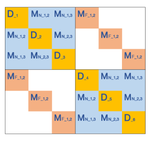
We now compare the KS (our model) and KP (model of [7]) structures when they are imposed in the coefficient of VAR(1) models. As mentioned before, when KP and KS structures are present in adjacency matrices, it implies in both cases that, the corresponding graphs can factorize into smaller graphs. To see the difference of factorization, let be the adjacency matrices of two graphs , then the KP and the KS are respectively the adjacency matrices of their tensor product graph and Cartesian product graph [28]. We illustrate these two product graphs in Figure 2555For the formal definitions of Cartesian and tensor products of graphs, we refer to Hammack et al. [15], Chen & Chen [8], Imrich & Peterin [18]..


Figure 2 shows that, the two product graphs differ greatly. For example, the lattice-like structure of the Cartesian product preserves the subgraphs in all sections of both dimensions. By contrast, the tensor product focuses on the cross-dimensional connection, yet abandoning the intra-dimensional dependency. This later property actually refers to, in the Gaussian process literature, the cancellation of inter-task transfer, see for example, Bonilla et al. [4, Section 2.3]. Therefore when the nodes represent , imposing KP structure [7] implies assuming no causality dependencies among for each fixed, which represent the observations of the feature at different nodes across the network. By contrast, the coefficient matrix of KS structure is able to take such dependencies into account during inference, which are in effect present in many applications. This justifies our choice.
3 Online Graph Learning
In this section, we develop two learning frameworks to estimate recursively. The first method is valid in low dimensional regime, where the number of samples along time is assumed to be sufficiently large with respect to the number of parameters. By contrast, the second method based on a Lasso-type problem requires fewer samples, and it is thus adapted to high-dimensional regime. We especially consider a general learning framework where the partial sparsity is pursued in the estimation of only . This is motivated by the fact that, merely a very small number of features are usually present in applications. Thus, the feature graph can be reasonably assumed fully-connected. On the other hand, since the partial sparsity constraint is also a technically more complicated case for the proposed high dimensional learning method, given its corresponding resolution, the adaption to the case of fully sparsity does not require novel techniques. In the following section, we firstly introduce the tools on constraint set , which are crucial to derive the proposed frameworks.
3.1 Orthonormal Basis and Projection Operator of
defined as Equation (2.7) is a linear space of dimension . We now endow with the Frobenius inner product of matrix, that is . The orthogonal basis of is then given in the following Lemma.
Lemma 3.1.
The set of matrices , defined below form an orthogonal basis of
| (3.1) |
where when , , when , is almost a zero matrix except
| (3.2) |
when , is almost a zero matrix except
| (3.3) |
In Figure 3, we give an example of this orthogonal basis of for , where are visualized with respect to their non-zero entries.
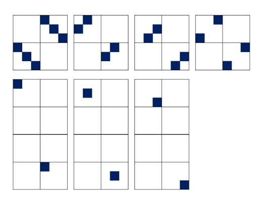
We can find that each relates to one variable of and , and characterises how it contributes to the structure of by repeating at multiple entries. Thus, taking the inner product with actually calculates the average value of an arbitrary matrix over these entries. This is important to understand how to project an arbitrary matrix onto .
It is easy to verify that for any in , and spans . Thus the normalized matrices form an orthonormal basis of . We introduce the orthogonal projection onto and provide an explicit formula to calculate it using in Proposition 3.2.
Proposition 3.2.
For a matrix , its orthogonal projection onto is defined by
| (3.4) |
Then given the orthonormal basis , the projections can be calculated explicitly as
| (3.5) |
The projection is very straightforward to understand. To obtain a variable in and related to , we use to calculate the average value of as explained previously. Then this average value is put at the corresponding entries to construct the structure, by multiplying locator .
Furthermore the orthogonality of the basis implies the direct sum
| (3.6) |
where , , and are respectively spanned by , , and . Given the construction of , Equation (3.6) actually reveals the product graph decomposition, note that equally we have
The projection onto these subspaces can also be computed analogously
| (3.7) |
| (3.8) |
| (3.9) |
We use and to denote the small matrices and , with an extra subscript , with which we will represent the proposed estimators of in the following sections. Finally, we have
| (3.10) |
3.2 Approach 1: Projected OLS Estimators and Wald Test
In low dimensional regime, Model (2.4) can be fitted by the ordinary least squares method as a VAR model. Assume that we start receiving samples from time , the OLS estimator for an intercept-free VAR() model is given by
| (3.11) |
where
and
respectively estimate the auto-covariance matrices and , with .
The classical results [21, Section 3.2.2] show that the OLS estimator of a stationary VAR model is consistent, moreover, permits a central limit theorem (CLT), if the following assumptions are satisfied.
Assumption 3.3.
-
1.
The white noise is independent, namely, .
-
2.
The white noise has singular covariance, and bounded fourth moments.
-
3.
The initial sample is already drawn from a stationary model, in other words, it permits the causal representation .
Given Assumption 3.3 and the stationary condition 2.1, the classical results show that
-
1.
,
-
2.
, where ,
where is the true coefficient which has the structure of .
However, in practice, due to model misspecification and limited samples, will not have the same structure as . Because the structure is crucial to retrieve the inferred graphs. We propose to perform the projection of onto , which leads to the projected OLS estimator:
Given the representation (3.10), it is natural to define the estimators of , , and by , , and , respectively, denoted by , , and . We now establish the Wald test with to identify the sparsity structure of the true . To this end, we provide the CLT in Theorem 3.4.
Theorem 3.4.
The proof is done through applying Cramér-Wold theorem on , given the linearity of and the CLT of classical OLS estimator . For details, see Appendix A, where we also derive a CLT for .
It is straightforward to understand the asymptotic distribution of . The asymptotic covariance between its two entries is assigned the mean of covariance values , following the construction of the corresponding estimators and as averages as well.
Based on this large sample result, to retrieve the sparsity structure of , we now test the nullity of given variables , with as
where . The test statistic is given by
| (3.13) |
where , and is defined as
such that is the matrix corresponding to variable ,
are the consistent estimators. CLT (3.4) implies the following result.
Corollary 3.4.1.
The asymptotic distribution of as is given by
Remark 1.
We can also consider the test statistic as suggested in Lütkepohl [21, Section 3.6] in conjunction with the critical values from .
Remark 2.
In practice, the significance level of test is a hyperparameter which can control sparsity of the estimator.
The Wald test above theoretically completes the approach. In practice, we propose to test the entries of the smallest estimate magnitudes, jointly each time, as grows from to possibly largest value . Specifically, for a given estimation , we first sort its entries such that
Then, we set up the sequence of joint tests
We perform these tests sequentially until is rejected for some . Lastly, we replace the entries with in as the final estimate of . Note that searching for resembles root-finding, since the output from each point is binary. Thus, the search can be accelerated by using the bisection, with the maximal number of steps about .
The previous procedure is performed at the -th iteration, given the OLS estimator and the consistent estimator . When new sample comes, and can be calculated efficiently by applying Sherman Morrison formula on . The pseudo code is given in Algorithm 2.
3.3 Approach 2: Structured Matrix-variate Lasso and Homotopy Algorithms
As discussed at the introduction, a common practice in the literature to identify the sparsity structure of VAR coefficients in high dimensional regime is to adopt Lasso estimators. The one used in Bolstad et al. [3], Zaman et al. [36] is defined as the minimizer of Lasso problem (3.14) in the VAR() case.
| (3.14) |
where is a vector of sample, which can be taken as for example. Lasso (3.14) is the most standard Lasso in literature [16, Section 3.4.2]. A wide variety of frameworks from convex analysis and optimization have been adapted to compute its solutions for different scenarios, for example, coordinate descent [12], proximal gradient methods [2], and a more Lasso-specific technique least angle regression [10]. However, Lasso (3.14) is not able to estimate the structured with the sparse component . Therefore motivated by the estimation, we propose the novel Lasso type problem (3.15)
| (3.15) |
We can see that the proposed Lasso problem differs from the classical Lasso (3.14) by the structure constraint and the partial sparsity regularization on instead of on all parameters . The ordinary resolution of Lasso (3.15) can be done by applying for example the proximal gradient descent [27]. In the algorithm framework, the structure constraint and the partial sparsity do not pose additional difficulties, since only the gradient with respect to is calculated in the forward step. We show these details in Appendix E.
At this point, we focus on providing the algorithms to quickly update the previous solutions for the change in the hyperparameter value or in the data term. This different goal requires to consider specific methods. For classical Lasso, the framework of homotopy continuation methods [26] has been explored [22, 13] to calculate the fast updating. Since the homotopy algorithm is derived from the optimality condition, which is with respect to the matrices in for Lasso (3.15), requiring to consider the gradient with the structure, thus the existing homotopy algorithms for classical Lasso are not applicable. Therefore in the following, we first calculate the optimality condition of Lasso (3.15) in Section 3.3.1, based on the expression of projection onto . Then we derive the two homotopy algorithms in Sections 3.3.2 and 3.3.3, respectively for the updating paths and , together with an adaptive tuning procedure for the regularization hyperparameter.
Therefore, the online algorithm consists in performing the three steps in the order:
| (3.16) | ||||
3.3.1 Optimality Conditions
The key point in deriving the optimality conditions arising from the variational problem (3.15) is to transfer the structure of onto the data vector , using an orthonormal basis of . We introduce the auxiliary variable , such that , and rewrite Problem (3.15) with respect to
| (3.17) |
Problem (3.17) is weakly convex, since a minimizer of (3.15) can be projected from infinitely many minimizers of (3.17). We still use to denote the objective function above. A minimizer of (3.17) satisfies the optimality conditions
| (3.18) | ||||
Assume is a matrix which satisfies Equation (3.18), hence a minimizer of Problem (3.17). Then is a minimizer of Lasso (3.15). We denote its active set by , that is all the non-zero variables of , and its non-active set by , that is . Since is an orthogonal family, Equation (3.18) is equivalent to
| (3.19) |
| (3.20) | ||||
| (3.21) | ||||
The optimality conditions above are an extension of those for classical Lasso. Compared to the conditions of classical Lasso which are given by two linear systems, ours are furthermore refined to three corresponding to the addition situation where a subset of variables in the problem are not penalized.
3.3.2 Homotopy from to
To develop the homotopy algorithm for the change in value, we need to get the formulas of the active variables indexed by in terms of . To this end, we firstly reorganize all the model variables into a vector
Note that is in fact the scaled Lasso solution by the time the variable repeats. Then optimality conditions (3.19), (3.20), and (3.21) are essentially a system of linear equations of unknown , with in the coefficients. Thus we aim to firstly represent this linear system in vector form, in order to solve the unknowns. We shall introduce the following notations.
Notations of Proposition 3.5.
is a large matrix defined as
is a long vector defined as
is a long vector where is defined as
| (3.22) |
We define , that are all the non-zero variables. Note that except the computational coincidence, the variables in are usually non-zero. Then we denote the extractions
| (3.23) | ||||
We can endow any orders to the elements in to extract the rows/columns/entries above, only if the orders are used consistently to all the extractions. With these notations, we now can retrieve a system of linear equations from Equations (3.19), (3.21), (3.20) of unknowns . Each equation is obtained by equating the entries of one . The resulting system is given in Proposition 3.5.
Proposition 3.5.
A minimizer of Lasso problem (3.15) satisfies the linear system
| (3.24) |
The representation of the optimality conditions in Equation (3.24) are similar to those of classical Lasso [13, 22], where , with the embedded structures correspond to , in the optimality conditions of classical Lasso. However in our case, the non-zero and sign pattern are only with respect to the entries of , thus , which is the equivalent of sign vector, has zeros.
Suppose that is the unique solution for a fixed of the optimization problem (3.15), then we invert in Proposition 3.5 and get the formulas of
| (3.25) |
Formula (3.25) is determined by the active set and the sign pattern of the optimal solution at . It shows that is a piecewise linear function of , while is also a piecewise smooth function.
Therefore, with the assumptions that (element-wise), and (element-wise), due to continuity properties, there exists a range containing , such that for any , element-wise, remains nonzero with the signs unchanged, and remains in . Hence, Formula (3.25) is the closed form of all the optimal solutions , for . are taken as the closest critical points to . Each critical point is a value which makes either an become zero, or a reach or . By letting and in Formula (3.25), we can compute all critical values. We now use to denote the orders of that we used in the extraction (3.23). The critical values are then given by
| (3.26) | ||||
Thus, the closet critical points from both sides are
| (3.27) | ||||
If then , while if then . After leaves the region by adding or deleting one variable to or from the active set, we update in order the corresponding entry in , , and the solution formula (3.25) (Sherman Morrison formula for one rank update of ) to calculate the boundary of the new region as before. We proceed in this way until we reach the region covering the value at which we would like to calculate the Lasso solution, and use Formula (3.25) in this final region to compute the with the desired value. Lastly, we retrieve the matrix-form optimal solution based on and the latest . This completes the first homotopy algorithm. The detailed algorithm see Appendix G.
3.3.3 Homotopy from to
We recall again the classical Lasso in Equation (3.28). We formulate it with vectorial parameter here.
| (3.28) |
where , , and are the samples at time . Garrigues & Ghaoui [13] propose to introduce a continuous variable in Lasso (3.28), leading to the optimization Problem (3.29)
| (3.29) |
in order to let the problem of learning from samples evolve to that of learning from samples, as goes from to . Therefore, representing the Lasso solution as a continuous function of permits the development of homotopy algorithm, which computes the path to .
This homotopy algorithm is derived based on the fact that, the term of new sample will only result in a rank-1 update in the covariance matrix as , because only response variable is present. Thus, the corresponding matrix inverse in the closed form of optimal solution can be still expressed as an explicit function of using the Sherman Morrison formula, which furthermore allows the calculation of critical points of . However, for the matrix-variate Lasso (3.15), a new sample will cause a rank- update666On the other hand, this implies that will quickly become non-singular from the initial time, as new samples come in. in , that is the number of response variables in the Lasso problem 777More general, a new sample will cause rank change in the corresponding matrix in Lasso (3.14).. To formally understand this change, we rewrite as the sum of reorganized samples analogous to usual
note that a new corresponds to the change in , which is a rank matrix. Thus it is impossible to express as an explicit and simple function of one single . However, note that each column (rank) corresponds to introducing new sample of one response variable at node in , by rewriting the incremental term of Lasso (3.15)
| (3.30) | ||||
Therefore, we propose to introduce continuous variables in Lasso (3.15), and to consider the following problem
| (3.31) | ||||
Given solution , we first apply the homotopy Algorithm of Section 3.3.2 on it with and to change the constant before the old data term from to . Then, we have and . We let evolve the optimization problem (3.15) from time to by sequentially varying all from to , along the paths
Proposition 3.6.
The optimal conditions given in Proposition 3.6 show that, each path only relates to the one rank change: , for the latest updated . Thus we can apply the Sherman Morrison formula on to retrieve the smooth function of , and express and as smooth functions of , which furthermore makes the calculation of the critical points of explicit. To leverage these continuity properties, we still assume (element-wise), and (element-wise). For the algorithm of path to , it is sufficient to impose such assumption only on . By arguing as in Section 3.3.2, we can derive the homotopy algorithm for the whole data path. For details, see Algorithm 5 in the appendices.
3.3.4 Update from to
Given the previous solution , one way to select the hyperparameter value is to introduce the empirical objective function [25, 13], which takes the form
| (3.35) |
and to employ the updating rule
| (3.36) |
where is the step size. For convenience, we write as . Analogously, we adopt the notation to denote the derivative with respect to , taken at value . The objective function can be interpreted as an one step prediction error on unseen data. Since the Lasso solution is piece-wise linear with respect to , it follows that when is not a critical point, the derivative can be calculated as
| (3.37) | ||||
where is defined as , with , , associated with , and
The derivatives of the entries of indexed by at can be calculated through the formula (3.25) of . By contrast, the derivatives of the entries of indexed by all equal zero. To obtain the non-negative parameter value, we project onto interval by taking , whenever the result from Equation (3.36) is negative.
Note that defined in Equation (3.36) can be interpreted as the online solution from the projected stochastic gradient descent derived for the batch problem
| (3.38) |
Therefore, the sublinear regret property of projected stochastic gradient descent implies that, when is given as , we have
| (3.39) |
Equation (3.39) implies that in the sense of average one step prediction error defined as Equation (3.38), the adaptive hyperparameter sequence will perform almost as well as the best parameter , for a large number of online updates, with sufficiently small step size . This completes the online procedure in the high dimensional domain, which we conclude in Algorithm 1.
4 Augmented Model for Periodic Trends
The online methods derived previously are based on the data process (2.4), which assumes the samples have the time-invariant mean zero. In this section, we propose a more realistic data model which considers the trends, and adapt the online methods for stationary data to this augmented model.
In literature of time series analysis, stationarity is very often taken as part of model assumptions due to its analytic advantage. Meanwhile the raw data usually is not stationary, for example Figure 1. In Figure 4, we show moreover a comparison of stationary time series and non-stationary time series.
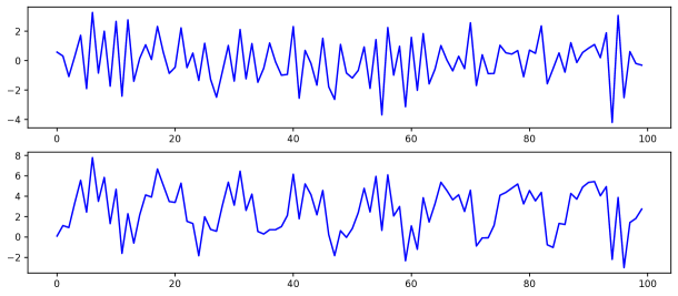
Thus in offline learning, to fit the models on data, a detrend step is needed, which approximates the trend function using the entire data set, then removes it from the raw data. However, since the principle of online learning does not require the presence of all data, such pre-processing step is forbidden. Thus, we need to consider the trend as the explicit parameters additional to the graph parameters in the online model. We propose the following augmented model
| (4.1) |
where , , with non-singular covariance matrix and bounded fourth moments, and . The observations of Model (4.1) is , while has the similar role as the unobserved state in the state space models however the observation equation here is much simplified. Therefore the estimators are built on the series . Note that Model (4.1) admits another reparameterization with intercept
| (4.2) |
The augmented model assumes that the non-stationarity of the observations is caused by the trend . We consider in particular in this work, the periodic trend
| (4.3) |
where is the length of period and it is a hyperparameter to be preassigned. This type of trend is frequently encountered in practice. For example, an annual recurrence () can be found in many monthly data sets recorded over years, such as the weather data in Figure 1. In the following sections, we will adapt the two learning frameworks presented in Section 3 to the augmented model for the periodic trends, in order to infer the trends and graphs simultaneously from non-stationary time series , in an online fashion.
4.1 New OLS Estimators and Asymptotic Distributions
For the augmented model (4.1), we propose a new OLS estimator of , which is based on the new sample auto-covariances, together with the OLS estimator of . Because two crucial properties to derive the Wald tests in Section 3.2 are the consistency of sample auto-covariances , and the CLT of OLS estimator , we derive the corresponding asymptotic results for the new estimators, and show that these asymptotics are exactly the same as in the stationary case. Therefore, all the results and procedures presented in Section 3.2 can be applied directly on the new estimators. We first define the estimator of , still denoted as , using general least squares (GLS) method
| (4.4) |
where
with , and the true white noise covariance given in Model (2.4). Note that represents the residual of the prediction of sample . The explicit forms of can be found through straightforward calculation, which yields new sample auto-covariances, denoted still as , and the estimator of trend . Specifically, we have
| (4.5) |
with
Note that denotes . It is also straightforward to understand the new auto-covariance estimators. Each leads to an OLS problem of regression equation (4.2). Its minimization introduces two sample covariance matrices. The weighted average of all such sample auto-covariance matrices for is the new sample auto-covariance for Model (4.1). denotes the number of times that the samples from the -th state point in the period have been predicted in the sense of Equation (4.4). As grows, becomes quickly, and becomes . For the augmented model, GLS and OLS estimators are still identical, with the latter defined as
The estimators given by Formula (4.4) enjoy the asymptotic properties in Proposition 4.1.
Proposition 4.1.
The following asymptotic properties hold for the estimators , as ,
-
1.
, ,
-
2.
, ,
-
3.
,
where , .
The proofs of the above results are given in Appendix B. Thus, Theorem 3.4 and the bisection Wald test procedure are still valid using and defined in this section. On the other hand, and satisfy the one rank update formulas
| (4.6) | ||||
where . Thus, when new sample comes, can still be calculated efficiently given the matrix inverse at the previous time. The details of the extended low dimensional learning procedure see Algorithm 3 in the appendices.
4.2 Augmented Structured Matrix-variate Lasso and the Optimality Conditions
To adapt the Lasso-based approach to Model (4.2), the corresponding trend and graph estimators can be obtained by minimizing the augmented Matrix-variate Lasso problem
| (4.7) |
As in the extension of our first approach, the extra bias terms do not affect the core techniques, rather they force the methods to consider the means in the sample autocovariances. Since only appear in the squares term, the minimizers have the same dependency with as in Equation (4.5). Thus the trend can still be estimated by , and we extend the algorithms in Section 3.3 to update the batch solution of augmented Lasso (4.7) from to , given new sample . To compute the regularization path , Proposition 4.2 implies that Algorithm 4 can still be used, with the adjusted definitions of and .
Proposition 4.2.
For the data path , in the same spirit of Problem (3.31), we introduce variables to let evolve Lasso problem (4.7) from time to through the following variational problem
| (4.9) | ||||
where , .
We recall that we update the solution along the path
At each step , the optimal solution is piece-wise smooth with respect to , element-wise. We retrieve the linear system of in terms of for the optimality condition of each in Proposition 4.3.
Proposition 4.3.
Therefore, the derived homotopy algorithm is essentially the previous homotopy Algorithm 5 with minor changes. For details, see Algorithm 6 in the appendices.
Lastly, we derive the updating rule for the regularization parameter. We still consider the one step prediction error, which writes as the following objective function in the case of Model (4.2)
| (4.11) |
Given the previous solution and , we assume that is not a critical point. Then the derivative of with respect to is calculated as
| (4.12) | ||||
where , . Analogous to Section 3.3.4, we have . Using the same updating rules of the projected stochastic gradient descent presented in Section 3.3.4, we can compute the online solution . We can see that, the introduction of bias terms into the original model makes them center the raw data automatically during the model fitting. This enables the direct learning over raw time series, while maintaining the performance of methods comparable to the stationarity-based ones.
We summarize the complete learning procedure of this subsection in Algorithm 6 in the appendices.
5 Experiments
We test the two proposed approaches for the online graph and trend learning on both synthetic and real data sets.
5.1 Synthetic Data
5.1.1 Evaluation Procedures
We now present the evaluation procedure for the augmented model approaches. In each simulation, we generate a true graph with the structure indicated by . In particular, we impose sparsity on its spatial graph by randomly linking a subset of node pairs. The values of non-zero entries in , and the entries in , are generated in a random way. Additionally, we generate a trend over a period of time points for each node and each feature. Therefore, the true , consists in these trend vectors, each containing elements. Then, observations are generated from Model (4.1), where the noise follows a centered multivariate normal distribution with a randomly generated covariance. Figure 4 shows an example of the synthetic time series , compared with its stationary source before adding the periodic trend. The graph and trend estimators proposed in Section 4 only use .
To start our two online procedures, we firstly synthesize very few samples until time . We set up the batch Lasso problem (4.7) with the generated samples and use its solution to start the high-dimensional online procedure since the next synthetic sample. The batch problem is solved via the accelerated proximal gradient descent with the backtracking line search [27, Section 3.2.2]. We especially set as a large number so as to have an over sparse initial solution. Therefore, we expect to see a decreasing , together with a more accurate estimate as grows. For the low-dimensional procedure, since it requires , we wait until there are enough samples, simply set as to start.
To analyse the performance of the proposed online estimators, we define the following error metrics. The average one step prediction error metric 999Note that, the prediction error is defined with the conditional expectation (i.e. the oracle best prediction) instead of the new observation . This is because we observed in experiments that due to the presence of the random noise, the oracle prediction can be less optimal than other empirical predictions. To avoid this misleading by the noise, we compare the proposed predictions with the oracle best prediction to evaluate their performance. On the top of it, we do not use the direct prediction error at each step in the metric, because the corresponding metric curves are shown very noisy in practice. To facilitate the graphical presentation, we take additionally a moving average, as shown in Equation (5.5). is given as
| (5.1) |
and root mean square deviation (RMSD) as
| (5.2) |
where denotes the estimates from either approach at time , and
| (5.3) |


Given the error metrics, we collect their values along time. We perform such simulation multiple times to obtain the means and the standard deviations of error metrics at each iteration (when the estimators are available) to better demonstrate the performance. The true graph and trends are generated independently across these simulations.
To furthermore justify the proposed models, we implement additionally the MAR models of [7] and the classical VAR(1) models in the simulations above. Especially, [7] proposed estimators for their KP-based MAR models, which we will all test. For the VAR(1) models, we use the OLS estimation. To make the comparison fair, we perform another group of simulations where samples are generated from the MAR models of [7]. To be more specific, in each simulation of the second group, we first generate the KP component and randomly. and are imposed no sparsity nor symmetricity. On the other hand, we randomly generate trend vectors, all over a period of time points. Then we synthesize latent stationary samples according to Model (1.9), where the noise follows a centered multivariate normal distribution with a randomly generated covariance. Afterwards, we add the periodic trends to the stationary samples to generate the synthetic observations. Therefore for this group of simulations, the coefficient matrix in the prediction error metric (5.5) should be , and the intercepts bm(τ+1) should be modified accordingly. The true model parameters are generated independently across the simulations.
For the second group, we start our online procedures the same way and at the same time as before. The procedures are applied directly on the observed time series, even though they are generated from the model of [7]. We present how to start the competitor estimators in both groups. On one hand, because they are designed for stationary time series and are all offline methods, we need to calculate them anew at each time step and with a pre-processing detrending step. The detrending step we adopt is the same one used in the numerical experiments of [7, Section 5.2]. The estimation of (periodic) trends in the detrending step is used therefore to calculate the prediction error metric for the competitor methods by replacing and . On the other hand, the competitor estimators do not have extra regularization as the Lasso one in our case, so they are not available101010This means that they are not calculable or the corresponding algorithms can not converge. as immediate as our high-dimensional estimator. Thus for the OLS estimator of VAR(1) model and the projection (Proj) estimator of [7], we start calculating them from the same time as our low-dimensional estimator. For the iterated least squares (MLE) and the structured maximum likelihood (MLEs) estimators of [7], we check at each step and record them whenever they are available.
5.1.2 Simulation Results
To facilitate the remarks, we organize this section in two parts. In the first part, we report the performance of our methods without comparing to the competitors and focus on its interpretation. In the second part, we examine our methods in comparison with other methods.
In the following, we visualize the representative estimates in heatmap with , , and for illustration purpose. Then we plot the evolution of error metrics and regularization parameter of simulations for , , and . Lastly, we report the running time. The hyperparameter settings are given in the captions of figures of corresponding results.
Figures 5 and 6 show the estimated graphs of two approaches when their corresponding online procedures start. In Figure 5, we can see that the batch solution which starts the high-dimensional procedure is over sparse due to the large . We can notice from Figure 6 that the two initial estimations of are already satisfactory, especially the Lasso solution which uses only samples. Actually, estimations of and converge to the truth very quickly in both cases when is significantly larger than . Figures 7 and 8 show that the estimations of of both approaches tend to the true values as more samples are received. Meanwhile, Figure 9 shows the effectiveness of trend estimator defined in Equation (4.5).


We now show the numeric results of simulations, with , , and . We test three different step sizes , , , and . With each value we perform independent simulations. Figure 10 and 11 plot the evolution of error metrics (5.5) and (5.2), respectively. For better visualization effect, since the performance of the low-dimensional procedure does not depend on , we only show one mean metric curve instead of , in the two figures, which is calculated from the results of these simulations.
Figure 10 shows the evolutions of estimator errors of the true coefficient . Overall, we can see that the step size influences the convergence speed of the high-dimensional estimators. Specifically, the RMSD of the high-dimensional estimator with converges the most quickly for the first samples, after which it starts to slow down and decrease more slowly than the RMSDs of the other two step sizes. For the low-dimensional estimator, when it is available, the RMSD decreases very fast and faster in higher dimension than those of high-dimensional estimators. This was expected, because the regularization in the high-dimensional estimator will cause bias, while the low-dimensional estimator is consistent as we showed in Theorem 4.1 and the comments below.
The impact of the step size is not significant in terms of the prediction error as shown in Figure 11., possibly because the latter aggregates the estimator error of with other quantities such as the samples and the estimator error of trend. Besides, it shows that the prediction error of the low-dimensional estimator is worse than that of the high-dimensional one. This follows the fact that the estimator error of the former is worse almost all the time during the testing period, even though it starts to descend faster at the end.
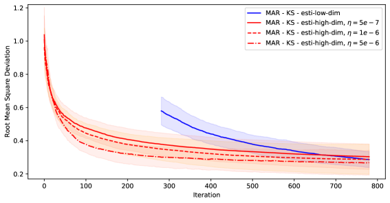
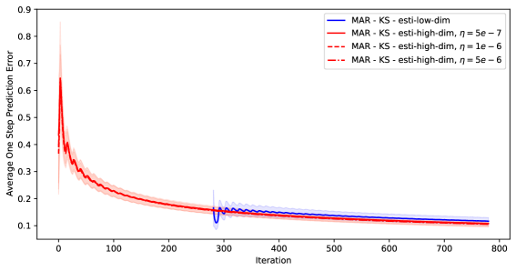
For synthetic data, it is not surprising that the RMSD from the low-dimensional procedure will tend toward zero, because these data are precisely sampled from the model used in the method derivation. On the other hand, at each online iteration, the OLS estimation is calculated accurately. In contrast, for the homotopy algorithms, they still introduce small errors, possibly due to the following assumptions used in the derivation of the method: 1. the active elements of of the algorithm inputs are not zero111111This hypothesis means that, some zero should not satisfy the first equations of the optimality condition (3.24) and (3.32), due to the computation coincidence.; 2. the sub-derivatives of those zero elements are strictly within ; 3. every at which we calculate the derivative as in Section 3.3.4 is not a critical point. Thus, for example, small non-zero entry values in the inputs may cause the numerical errors. However, in real applications, the only available metric which allows the performance comparison is the prediction error (5.5).
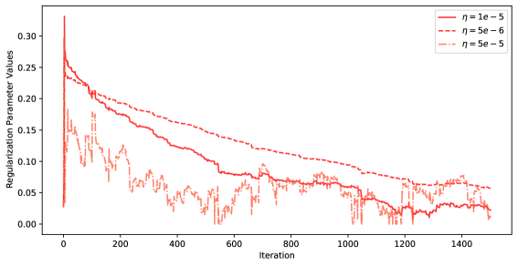
Figure 12 demonstrates the performance of the updating method of the regularizing parameter , and the impact from different step size values . The curves emphasize the convergence of the estimation updated by the high-dimensional procedure. Moreover, we can observe that all three are decreasing, which was expected from the experiment design. On the other hand, the results show again that a larger step size will make the convergence faster. In this figure, we can observe additionally curves of larger steps are noisier.
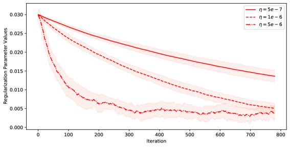
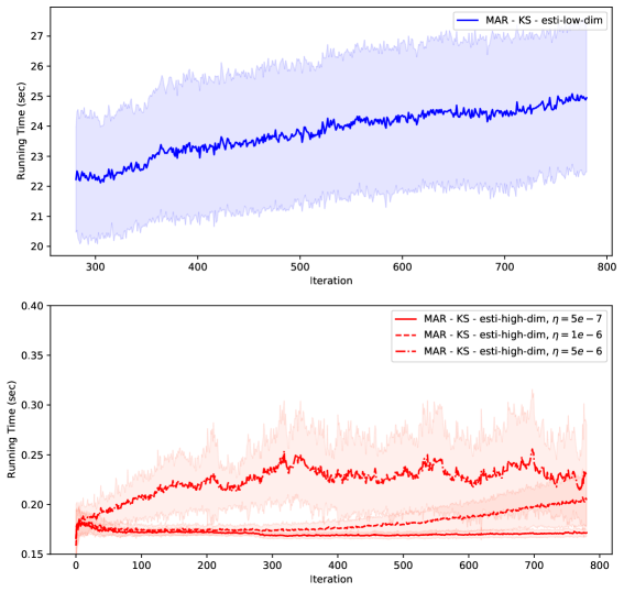
For our approaches, we also record the running time of their online updates in Figure 13. Firstly, it is clear that updating the Lasso solutions by the homotopy algorithms saves considerable time, which is on average seconds for the graph size , . The running time of the accelerated proximal gradient descent performed in the beginning of these simulations costs more than seconds. By contrast, an update using the low-dimensional procedure takes seconds on average. We can also notice that the high-dimensional procedure with larger step size runs slower, because the updated regularization parameter is quite different from the preceding one, as evidenced by the results in Figure 12. This aspect of evaluation is not used for the competitor methods. The reason is three-fold. Firstly, the computation time for the methods of [7] depends on the stopping criteria of the corresponding algorithms, which simultaneously impact the performance of methods. Thus it is difficult to set ideal stopping criteria which allow us to compare both performance and running time. Secondly, they do not consider sparsity in estimation, thus the calculation of their estimators consists in nature fewer steps. Lastly, our way to code their algorithms also impacts their running time. Thus, we focus on the comparison with the performance by setting the stopping criteria sufficiently strict.
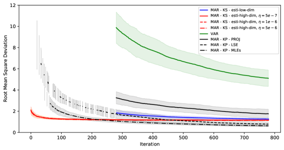
Now we move onto the results of the competitors. Figures 14, 15, and 16 report their estimation and prediction performance in comparison with ours. Firstly, in Figure 14, we can see that our estimators outperform the rest four estimators. Note that our low-dimensional estimator (blue) is the projected OLS estimator (green), thus the green curve represents in effect a consistent estimator. However since it is not applied techniques to reduce the dimensionality, in a fairly long period of our simulations, it can not beat the other estimators. This numerically evidences our claim in the introduction that vector models with reasonable structures in parameters are preferable than the direct use of vector models. Note that the KP structure is not the correct parameter structure in the true sample model, but it is still related to the KS structure.
Between our methods and those of [7], since the true model is not fair to the latters, we focus on the minimal sample sizes required by different methods. Firstly, our low-dimensional estimator and the Proj estimator of [7] are both projected OLS estimators. Thus they are not available before the matrix is invertible. The LSE estimator of [7] is defined through the following LS problem
It is solved by a proposed coordinate descent algorithm, which iterates between
| (5.4) | ||||
Thus the LSE estimator is not available before the matrix and the matrix are both invertible. In Figure 14, we can see the LSE estimator starts later than our high-dimensional estimators. To avoid inversing matrices in calculation, other algorithm frameworks could replace the coordinate descend, such as projected gradient descend. Such way, a (local) minimiser is calculable since the beginning. However, it still can not fix the instability problem. With regard to this point, we can also find in the figure that, the calculable LSE estimators121212Since each RMSD curve represents the mean of RMSD values at each time from multiple simulations. A missing value at a given time implies that the corresponding estimator is not available in one of the simulations at that time. before samples actually have large error mean and variance. To have better performance in high dimension, extra regularization is needed. The MLEs method also estimates directly the KP components and , thus similarly to the LSE method, the estimator is available in a higher dimension than the Proj one. Nevertheless, it estimates additionally the covariance of the noise, which is limited to have a KP structure as well. The authors supplemented the previous coordinate descend (5.4) algorithm by extra steps, the latter requiring to inverse more matrices. We can see in Figure 14 that the MLEs curves appears later than the MLEs one, but still more earlier than the low-dimensional estimators.
We also point out the reason which results in the jumps of LSE and MLEs curves at the starting time of the low-dimensional estimators. The two estimators are calculated by algorithms which can only converge to local minimizers, thus the solutions depend on the initial values. In the paper [7], it is suggested to use the Proj estimation. However we consider higher dimension, thus before the Proj estimation is available, we use other initial values (identity matrices), the change of initialization causes the jumps.
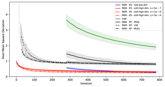
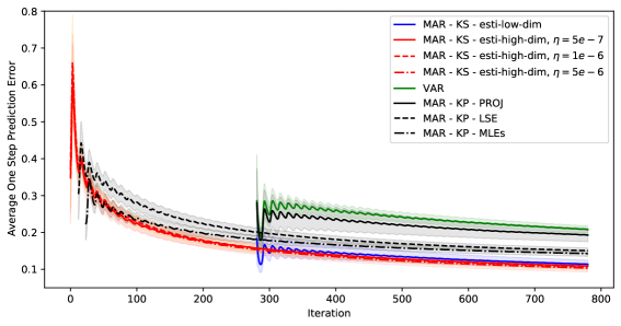
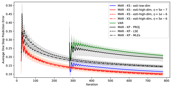
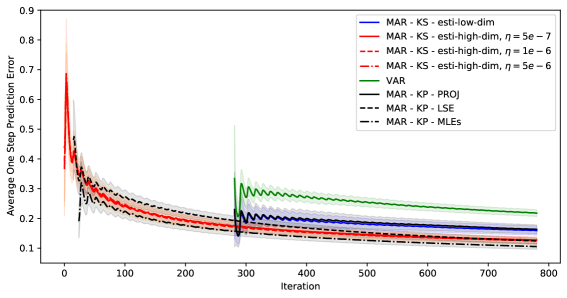
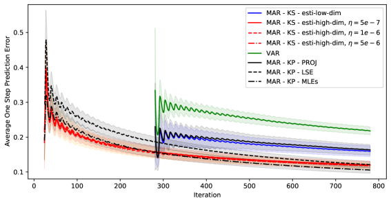
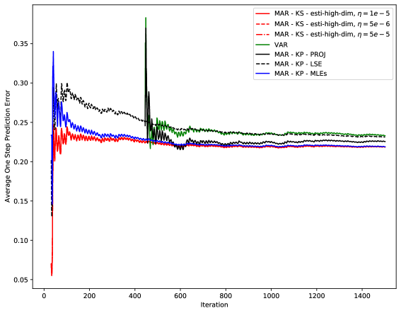
Figure 15 reports the prediction errors131313To calculate the curves for LSE and MLEs estimators, we take the moving average by ignoring the unavailable estimations occurred occasionally in the past. If the estimation is not available for the whole past with respect to a given time, the error metric is given Nan for that time. of different methods. We can see the prediction errors differ in the same way as the estimation errors, except that around samples, the LSE and MLEs methods slightly surpass our high-dimensional method. This is because the error metric is a moving average, thus its value at a given time aggregates all the past ones. Since the high-dimensional method is the only method which can work with extremely small sample sizes, on the other hand, smaller sample size leads to worse performance in general, these inferior errors of our estimator then propagate in longer period. Therefore, we plot additionally Figure 16, where we re-calculate the prediction errors for our high-dimensional and the LSE methods by not considering their errors which are available earlier than the MLEs method. We can see that the high-dimensional method actually outperforms the LSE and MLEs for all sample sizes.
In the previous group of simulations, both our high and low dimensional estimators outperform the competitors. The high-dimensional one is additionally more advantageous in terms of required sample size. These results are partly linked to the fact that the true sample model is ours. Now we report the results with samples generated by the MAR model of [7]. Firstly, Figure 17 shows that even with the unfair sample model, our high-dimensional estimator gives still the best estimation error in high dimension, then is beaten by the MLEs estimator around samples, and by the LSE estimator around samples. As for the Proj estimator, it is not able to beat our high-dimensional estimator within the testing period, because it relies on the performance of the OLS estimator of VAR model.
Next, Figures 18 and 19 report the prediction performance of methods. Same conclusion can be made as the estimation performance. From these simulations, we can see that the instability brought by the insufficient samples is more harmful than the model misspecification, which emphasizes the use of enough regularization in high dimension.
5.2 Climatology Data
In this section, we consider a real data set, which comes from the U.S. Historical Climatology Network (USHCN) data141414The data set is available at https://www.ncdc.noaa.gov/ushcn/data-access. The data set contains monthly averages of four climatology features, recorded at weather stations located across the United States, over years. The four features are: minimal temperature, maximal temperature, mean temperature, and precipitation. A snippet of the data set has been given in Figure 1, which illustrates these feature time series observed from a certain spatial location. A clear periodic trend can be seen from each scalar time series, with period length equal to months. We can also notice that some observations are missing in the data set; to focus on the evaluation of learning approaches, we do not consider the stations with incomplete time series. Geographically, we picked data only from California and Nevada for this experiment. The summary of experiment setting thus is: , total number of time points = months (covering the years from to ).
With this data set, we evaluate our methods from two aspects: as graph learning methods, we visualize the learned graphs and interpret them; as a new AR model, we compare the prediction error with the competitors. There is a third aspect of our methods which is as online algorithms. The corresponding evaluation does not depend on the nature of data. In effect, for the running time of online update, we have already tested and reported the performance in Figure 13. On the other hand, it is self-explained that our estimators do not need to store the past samples to be updated.
To compare the prediction errors, because we do not have the “true” model for real data, we use the following metric formula instead of the formula (5.5)
| (5.5) |
All methods are started the same way and same time as in the simulations. For our high-dimensional methods, we still set the initial as . The value does not affect the performance of high-dimensional method much, because of the adaptive tuning procedures.
5.2.1 Real Data Results
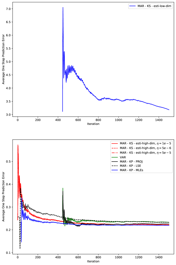
We first report the prediction errors in Figures 20 and 21. To have a better visual presentation, we report the curve of our low-dimensional estimator in a separate subfigure. We can see that it does not perform as well as in the simulations. A possible reason can be that it fairly relies on asymptotic results, thus it is less robust to model misspecification, especially data generating models for real data are more complicated than the two MAR models, more often are implicit. By contrast, our high-dimensional estimators still outperform the rest methods for all time steps, as shown in particular by Figure 21. We tested three different values of step size, they do not have significant impact on the prediction performance of the estimator as before. Comparing the counterpart results from simulations in 19 and 16, we find that further the “true" data model is away from our proposed model, less impact the step size will has on the prediction error of the estimator. We also show the evolution of associated to the three step sizes in Figure 22. The same impact of step size on the evolution of can be found as in Figure 12.
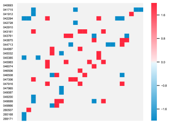
We now visualize the inferred graphs and trends from our methods. We report the results corresponding to since it has converged and is less noisy. Figures 23 and 24 show the spatial graphs learned by the two proposed approaches in Section 4 updated at different times. We can see that, for the high-dimensional method, when more observations are received, it finds that more location pairs actually have a Granger causal effect on each other. On the other hand, compared to the estimated graphs from the high-dimensional procedure, those from the low-dimensional procedure vary more along time.


Figure 25 shows the last updated feature graphs. We can see that the estimated feature relationships from the two approaches coincide in tmin and tmax, tmin and tavg, tmin and prcp. However, the relationship between tavg and prcp is very weak in the high-dimensional estimation, while strong in the low-dimensional estimation. Figure 26 reports the evolution of estimated trends from one representative spatial location along time, where we can observe the increase of temperature from the past to the present.

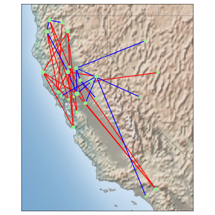
Lastly, in Figure 27, we plot the edge overlap (considering the signs of weights) of the two last updated spatial graphs, where we also visualize this spatial graph superimposed on the actual geographical graph. We can see that the remote weather stations have less dependency with other stations, while more edges appear within the area where lots of stations are densely located together. These observations imply that the inferred graphs provide the consistent weather patterns with geographical features.

6 Conclusion
In this paper, we proposed a novel auto-regressive model for matrix-variate time series with periodic trends. The model allows us to perform graph learning from matrix-variate time series, a data type which has not been considered yet in the literature on graph learning. Furthermore, such graph learning is online. This leads to our first aspect of contribution. Secondly, the proposed model enriches the family of matrix auto-regressive models, which is distinguished by its KS structure in contrast of the KP one used by the other MAR models. This distinction is justified by the experiments with both synthetic and real data. Thirdly, we extended the homotopy algorithms of classical Lasso to a new Lasso-type problem. The derived algorithms present an online learning framework, where the derivations do not depend on our specific structure assumed in . Note that the specific orthogonal basis, Equations (3.1), were not used in the rest technical sections. Instead, only the symbol of orthogonal basis, , were manipulated, as well as the symbol , indices of the bases which we wish to impose sparsity regularization. Thus the framework can be applied to the online inference of many other parametric models under structure and (partial) sparsity assumptions, as soon as the structure space is a linear subspace of the parameter space.
It is also of interest to point out that our MAR model can furthermore be extended for tensor-variate time series. The extension principle that we described in the introduction still works. One can first vectorize the data tensor, and apply the classical VAR models. Then, appropriate structures are imposed onto the coefficient matrices of VAR model. Based on VAR models, the Granger causality structure is still encoded by sparsity structure of the coefficient matrices. For instance, in the case of VAR models, an appropriate structure can be a multiway KS structure [33, 14] . Imposing such structure amounts to assuming that the total causality structure factorizes into smaller causal sub-graphs. At this point, sparsity of certain sub-graphs (modes of tensor) can be furthermore pursued in estimation. In the technical development, we only need to suppose the first sub-graphs are sparse. The value of and which modes of data tensor are made the first are to be specified freely by different applications.
Since the multiway KS structure still leads to a linear subspace of structured parameters, our estimators and the online procedures are all valid. We merely need to find the correct orthogonal basis for the new model, and assign a subset of indexed by which we wish to imposed the sparsity. Then we insert them into the proposed derivation to calculate the numerical results. Note that in this case, the fact that multiple sub-graphs are imposed the sparsity () regularization does not make difference. Because can still be expressed as , where contains the indices of the corresponding to entries of , thus Equation (3.17) is still valid. For low-dimensional, Wald test is originally performed independently for each sub-graph. This elaborated discussion has also demonstrated that the proposed inference framework is fairly generic. That completes the conclusion section.
Acknowledgments
Jérémie Bigot is a member of Institut Universitaire de France (IUF), and this work has been carried out with financial support from the IUF.
References
- Bach & Jordan [2004] Bach, F. R. and Jordan, M. I. Learning graphical models for stationary time series. IEEE transactions on signal processing, 52(8):2189–2199, 2004.
- Beck & Teboulle [2009] Beck, A. and Teboulle, M. A fast iterative shrinkage-thresholding algorithm for linear inverse problems. SIAM journal on imaging sciences, 2(1):183–202, 2009.
- Bolstad et al. [2011] Bolstad, A., Van Veen, B. D., and Nowak, R. Causal network inference via group sparse regularization. IEEE transactions on signal processing, 59(6):2628–2641, 2011.
- Bonilla et al. [2007] Bonilla, E. V., Chai, K., and Williams, C. Multi-task gaussian process prediction. Advances in neural information processing systems, 20, 2007.
- Bucci [2022] Bucci, A. A smooth transition autoregressive model for matrix-variate time series. arXiv preprint arXiv:2212.08615, 2022.
- Celani & Pagnottoni [2023] Celani, A. and Pagnottoni, P. Matrix autoregressive models: Generalization and bayesian estimation. Studies in Nonlinear Dynamics & Econometrics, (0), 2023.
- Chen et al. [2021] Chen, R., Xiao, H., and Yang, D. Autoregressive models for matrix-valued time series. Journal of Econometrics, 222(1):539–560, 2021.
- Chen & Chen [2015] Chen, S. and Chen, X. Weak connectedness of tensor product of digraphs. Discrete Applied Mathematics, 185:52–58, 2015.
- Dong et al. [2019] Dong, X., Thanou, D., Rabbat, M., and Frossard, P. Learning graphs from data: A signal representation perspective. IEEE Signal Processing Magazine, 36(3):44–63, 2019.
- Efron et al. [2004] Efron, B., Hastie, T., Johnstone, I., Tibshirani, R., et al. Least angle regression. Annals of statistics, 32(2):407–499, 2004.
- Friedman et al. [2008] Friedman, J., Hastie, T., and Tibshirani, R. Sparse inverse covariance estimation with the graphical lasso. Biostatistics, 9(3):432–441, 2008.
- Friedman et al. [2010] Friedman, J., Hastie, T., and Tibshirani, R. Regularization paths for generalized linear models via coordinate descent. Journal of statistical software, 33(1):1, 2010.
- Garrigues & Ghaoui [2008] Garrigues, P. and Ghaoui, L. An homotopy algorithm for the lasso with online observations. Advances in neural information processing systems, 21:489–496, 2008.
- Greenewald et al. [2019] Greenewald, K., Zhou, S., and Hero III, A. Tensor graphical lasso (teralasso). Journal of the Royal Statistical Society: Series B (Statistical Methodology), 81(5):901–931, 2019.
- Hammack et al. [2011] Hammack, R. H., Imrich, W., Klavžar, S., Imrich, W., and Klavžar, S. Handbook of product graphs, volume 2. CRC press Boca Raton, 2011.
- Hastie et al. [2009] Hastie, T., Tibshirani, R., Friedman, J. H., and Friedman, J. H. The elements of statistical learning: data mining, inference, and prediction, volume 2. Springer, 2009.
- Hsu et al. [2021] Hsu, N.-J., Huang, H.-C., and Tsay, R. S. Matrix autoregressive spatio-temporal models. Journal of Computational and Graphical Statistics, 30(4):1143–1155, 2021.
- Imrich & Peterin [2018] Imrich, W. and Peterin, I. Cartesian products of directed graphs with loops. Discrete Mathematics, 341(5):1336–1343, 2018.
- Kalaitzis et al. [2013] Kalaitzis, A., Lafferty, J., Lawrence, N. D., and Zhou, S. The bigraphical lasso. In International Conference on Machine Learning, pp. 1229–1237. PMLR, 2013.
- Li & Xiao [2021] Li, Z. and Xiao, H. Multi-linear tensor autoregressive models. arXiv preprint arXiv:2110.00928, 2021.
- Lütkepohl [2005] Lütkepohl, H. New introduction to multiple time series analysis. Springer Science & Business Media, 2005.
- Malioutov et al. [2005] Malioutov, D. M., Cetin, M., and Willsky, A. S. Homotopy continuation for sparse signal representation. In Proceedings.(ICASSP’05). IEEE International Conference on Acoustics, Speech, and Signal Processing, 2005., volume 5, pp. v–733. IEEE, 2005.
- Mei & Moura [2016] Mei, J. and Moura, J. M. Signal processing on graphs: Causal modeling of unstructured data. IEEE Transactions on Signal Processing, 65(8):2077–2092, 2016.
- Meinshausen et al. [2006] Meinshausen, N., Bühlmann, P., et al. High-dimensional graphs and variable selection with the lasso. Annals of statistics, 34(3):1436–1462, 2006.
- Monti et al. [2018] Monti, R. P., Anagnostopoulos, C., and Montana, G. Adaptive regularization for lasso models in the context of nonstationary data streams. Statistical Analysis and Data Mining: The ASA Data Science Journal, 11(5):237–247, 2018.
- Osborne et al. [2000] Osborne, M. R., Presnell, B., and Turlach, B. A. A new approach to variable selection in least squares problems. IMA journal of numerical analysis, 20(3):389–403, 2000.
- Parikh & Boyd [2014] Parikh, N. and Boyd, S. Proximal algorithms. Foundations and Trends in optimization, 1(3):127–239, 2014.
- Sandryhaila & Moura [2014] Sandryhaila, A. and Moura, J. M. Big data analysis with signal processing on graphs: Representation and processing of massive data sets with irregular structure. IEEE Signal Processing Magazine, 31(5):80–90, 2014.
- Songsiri & Vandenberghe [2010] Songsiri, J. and Vandenberghe, L. Topology selection in graphical models of autoregressive processes. The Journal of Machine Learning Research, 11:2671–2705, 2010.
- Sun et al. [2023] Sun, H., Shang, Z., and Chen, Y. Matrix autoregressive model with vector time series covariates for spatio-temporal data. arXiv preprint arXiv:2305.15671, 2023.
- Wang et al. [2024] Wang, D., Zheng, Y., and Li, G. High-dimensional low-rank tensor autoregressive time series modeling. Journal of Econometrics, 238(1):105544, 2024.
- Wang et al. [2020] Wang, Y., Jang, B., and Hero, A. The sylvester graphical lasso (syglasso). In International Conference on Artificial Intelligence and Statistics, pp. 1943–1953. PMLR, 2020.
- Wang et al. [2022] Wang, Y., Sun, Z., Song, D., and Hero, A. Kronecker-structured covariance models for multiway data. Statistic Surveys, 16:238–270, 2022.
- Wu & Chan [2023] Wu, F. and Chan, K.-S. Mixture matrix-valued autoregressive model. arXiv preprint arXiv:2312.06098, 2023.
- Wu & Bi [2023] Wu, S. and Bi, P. Autoregressive moving average model for matrix time series. Statistical Theory and Related Fields, pp. 1–18, 2023.
- Zaman et al. [2020] Zaman, B., Ramos, L. M. L., Romero, D., and Beferull-Lozano, B. Online topology identification from vector autoregressive time series. IEEE Transactions on Signal Processing, 69:210–225, 2020.
- Zhou [2014] Zhou, S. Gemini: Graph estimation with matrix variate normal instances. 2014.
Appendix A Proof of Results in Section 3.2 and the CLT for
Proof of Theorem 3.4. By Cramér-Wold theorem, is equivalent to
| (A.1) |
On the other hand, we can express the entries of as a linear function of
| (A.2) |
Then for all , we have
Let in Equation (A.1) be , then we have
Note that, Thus . Use Cramér-Wold theorem again, we can get the theorem result.
Theorem A.1.
(CLT for )
| (A.3) |
where .
Proof: The proof is similar as before. Because, we can express any entries of as a linear function of :
| (A.4) |
Thus, for all , we have
Let in Equation (A.1) be , then
Use Cramér-Wold theorem again, we can get the theorem result. The distribution in this theorem is degenerate.
Proof of Corollary 3.4.1. The proof is an adaption of Lütkepohl [21, Section 3.6]. We first construct the following matrix:
| (A.5) |
Then test versus equals to
Following CLT 3.4, we have
Hence, when holds,
Then by Proposition C.2 (4) in [21], we have
where is the consistent estimator of . Then by continuous mapping theorem:
Note that , and are orthonormal basis in , thus we have .
Appendix B Proof of Proposition 4.1
From Definition (4.5), we have
Plug in the last equation above, we can get the formula only with respect with
where , and . Note that .
(a’) , ,
(b’) ,
(c’) .
Thus, to reach the results in Proposition 4.1, we need additionally the asymptotic properties of sample mean , which are given in Lemma B.1.
Lemma B.1.
(CLT of )
where , and . Therefore, .
Proof of Lemma B.1. Because of the periodicity, is also a stationary process from VAR: , with , for all . Thus, apply Proposition in Lütkepohl [21], we get the result.
Proof of Proposition 4.1.
(a) When , , and , with .
(b) . Since asymptotically, , thus both means can be used to estimate . On the other hand, based on (a), using continuous mapping theorem on the matrix inverse, we have
(c) When , equals
Use Woodbury formula on the matrix inverse, we have
Based on the result of (c’), to reach the same asymptotic distribution, we only need to show that, the reminder terms, namely from the second term to the last term above, all converge to in probability.
Similarly, Since, it is obvious that , then use the properties of convergence in probability and continuous mapping theorem, we can show the reminder terms all converge to in probability.
Appendix C Bisection Wald Test for the Identification of Sparsity Structure of
Note that, since multiplication with amounts to extracting elements in the matrix from the corresponding locations, in practice, we take the elements directly from and , to compose as:
where , , , and , , with order indices , , , .
Appendix D Extended Algorithm 2 for the Augmented Model
Appendix E Proximal Gradient Descent for the proposed Lasso
The implementation of proximal gradient descent for Lasso (3.15) is given as follows.
| (E.1) | ||||
where , we denote by to avoid the heavy notation.
The forward step requires to calculate the gradient only in , then the backward step amounts to a classical Lasso after projecting the gradient onto . Thus the structure constraint and the partial sparsity do not pose additional difficulties.
Appendix F Matrix representation of the optimality condition of the proposed Lasso
The matrix representation of the optimality condition of Lasso (3.15) is given in terms of . To present it, we introduce the projections onto sub-spaces and , denoted respectively by and . Note that Equation (3.6) in fact admits
Thus
and
Then Equations (3.19), (3.20), and (3.21) are equivalent respectively to
| (F.1) |
| (F.2) |
| (F.3) |
where , , and .