All the attention you need:
Global-local, spatial-channel attention for image retrieval

Abstract

We address representation learning for large-scale instance-level image retrieval. Apart from backbone, training pipelines and loss functions, popular approaches have focused on different spatial pooling and attention mechanisms, which are at the core of learning a powerful global image representation. There are different forms of attention according to the interaction of elements of the feature tensor (local and global) and the dimensions where it is applied (spatial and channel). Unfortunately, each study addresses only one or two forms of attention and applies it to different problems like classification, detection or retrieval.

We present global-local attention module (GLAM), which is attached at the end of a backbone network and incorporates all four forms of attention: local and global, spatial and channel. We obtain a new feature tensor and, by spatial pooling, we learn a powerful embedding for image retrieval. Focusing on global descriptors, we provide empirical evidence of the interaction of all forms of attention and improve the state of the art on standard benchmarks.

1 Introduction

Figure 1: Our global-local attention module (GLAM) involves both channel and spatial attention, as well as both local attention (channels/locations weighted independently, based on contextual information obtained by pooling) and global attention (based on pairwise interaction between channels/locations). As a result, four attention maps are used: local channel ($\mathbf{A}_{c}^{l}$), local spatial ($\mathbf{A}_{s}^{l}$), global channel ($\mathbf{A}_{c}^{g}$) and global spatial ($\mathbf{A}_{s}^{g}$). The input feature map $\mathbf{F}$ is weighted into local ($\mathbf{F}^{l}$) and global ($\mathbf{F}^{g}$) attention feature maps, which are fused with $\mathbf{F}$ to yield the global-local attention feature map $\mathbf{F}^{gl}$. The diagram is abstract: The four attention modules are shown in more detail in Figures 2, 3, 4, 5.

Instance-level image retrieval is at the core of visual representation learning and is connected with many problems of visual recognition and machine learning, for instance metric learning [30, 26], few-shot learning [42] and unsupervised learning [8]. Many large-scale open datasets [3, 37, 16, 29, 53], and competitions have accelerated progress in instance-level image retrieval, which has been transformed by deep learning [3].

Many studies on instance-level image retrieval focus on learning features from convolutional neural networks (CNN), while others focus on re-ranking, for instance by graph-based methods [11]. The former can be distinguished according to feature types: local descriptors, reminiscent of SIFT [27], where an image is mapped to a few hundred vectors; and global descriptors, where an image is mapped to a single vector. In fact, deep learning has brought global descriptors with astounding performance, while allowing efficient search. Our study belongs to this type.

Studies on global descriptors have focused on spatial pooling [2, 37]. The need for compact, discriminative representations that are resistant to clutter has naturally given rise to spatial attention methods [24, 28]. Different kinds of attention have been studied in many areas of computer vision research. There is also channel attention [20, 9]; local attention, applied independently to elements of the representation (feature map) [54, 25]; global attention, based on interaction between elements [52, 9]; and combinations thereof. Unfortunately, each study has been limited to one or two kinds of attention only; attention is not always learned; and applications vary.

It is the objective of our work to perform a comprehensive study of all forms of attention above, apply them to instance-level image retrieval and provide a detailed account of their interaction and impact on performance. As shown in Figure 1, we collect contextual information from images with both local and global attention, giving rise to two parallel network streams. Importantly, each operates on both spatial locations and feature channels. Local attention is about individual locations and channels; global is about interaction between locations and between channels. The extracted information is separately embedded in local and global attention feature maps, which are combined in a global-local attention feature map before pooling.

Our contributions can be summarized as follows:

1. We propose a novel network that consists of both global and local attention for image retrieval. This is the first study that employs both mechanisms.

2. Each of the global and local attention mechanisms comprises both spatial and channel attention.

3. Focusing on global descriptors, we provide empirical evidence of the interaction of all forms of attention and improve the state of the art on standard benchmarks.

2 Related work

Instance-level image retrieval

Studies on instance-level image retrieval can be roughly, but not exclusively, divided into three types: (1) studies on global descriptors [3, 16, 24, 53, 2, 37]; (2) studies on local descriptors and geometry-based re-ranking [29, 45, 40, 53]; (3) re-ranking by graph-based methods [11, 21, 55]. The first two types of studies focus on the feature representation, while the last type focuses on re-ranking extracted features.

Studies on global descriptors focus on spatial pooling of CNN feature maps into vectors, including MAC [38], SPoC [2], CroW [24], R-MAC [48, 15, 16], GeM [37], and NetVLAD [1, 25], as well as learning the representation [3, 15, 16, 36, 37]. Studies before deep learning dominated image retrieval were mostly based on local descriptors like SIFT [27] and bag-of-words representation [32] or aggregated descriptors like VLAD [22] or ASMK [46]. Local descriptors have been revived in deep learning, e.g. with DELF [29], DELG [5] and ASMK extensions [45, 47].

Method	Local		Global		Lrn	Ret
	Spatial	Channel	Spatial	Channel
SENet [20]		✓			✓
ECA-Net [51]		✓			✓
GCNet [6]		✓			✓
CBAM [54]	✓	✓			✓
GE [19]	✓				✓
NL-Net [52]			✓		✓
AA-Net [4]			✓		✓
SAN [59]			✓		✓
N3Net [34]			✓		✓
A2-Net [9]				✓	✓
GSoP [14]				✓	✓
OnA [23]	✓					✓
AGeM [17]	✓					✓
CroW [24]	✓	✓				✓
CRN [25]	✓				✓	✓
DELF [29]	✓				✓	✓
DELG [5]	✓				✓	✓
Tolias et al. [47]	✓				✓	✓
SOLAR [28]			✓		✓	✓
Ours	✓	✓	✓	✓	✓	✓

Table 1: Related work on attention. LRN: learned; RET: applied to instance-level image retrieval.

We focus on learning a global descriptor in this work, because it is the most efficient in terms of storage and search. However, our generic attention mechanism produces a feature tensor and could be applicable to local descriptors as well, if global pooling were replaced by local feature detection. Re-ranking methods are complementary to the representation and we do not consider them in this work.

Figure 2: Local channel attention.

Attention

Attention mechanisms have been first proposed in image classification studies focusing on channel attention [20, 51, 6], spatial attention [19] or both, like CBAM [54]. In image retrieval, CroW [24] also employs both spatial and channel attention and can be seen as a precursor of CBAM, but, like other studies of spatial attention on retrieval [41, 23, 17], it is not learned. CRN [25] applies spatial attention for feature reweighting and is learned. Learned spatial attention mechanisms are common for local descriptors [29, 5, 47].

We call the above methods local attention, in the sense that elements of the feature tensor (channels / spatial locations), are weighted independently, based on contextual information obtained by pooling or learned. By constrast, by global attention we refer to mechanisms that model interaction between elements of the feature tensor, for example between channels or between locations.

In image classification, non-local neural network (NLNet) [52] is maybe the first global attention mechanism, followed by similar studies [4, 59, 34]. It is global spatial attention, allowing interaction between any pair of spatial locations. Similarly, there are studies of global channel attention, allowing interaction between channels [9, 14]. Global attention has focused mostly on image recognition and has been applied to either spatial or channel attention so far, not both. In image retrieval, SOLAR [28] is a direct application of the global spatial attention mechanism of [52].

Table 1 attempts to categorize related work on attention according to whether attention is local or global, spatial or channel, whether it is learned and whether it is applied to instance-level image retrieval. We observe that all methods limit to one or two forms of attention only. Of those studies that focus on image retrieval, many are not learned [23, 17, 24], and of those that are, some are designed for local descriptors [29, 47].

By contrast, we provide a comprehensive study of all forms of attention, global and local, spatial and channel, to obtain a learned representation in the form of a tensor that can be used in any way. We spatially pool it into a global descriptor and we study the relative gain of different forms of attention in image retrieval.

3 Global-local attention

We design a global-local attention module (GLAM), which is attached at the end of a backbone network. Figure 1 illustrates its main components. We are given a $c\times h\times w$ feature tensor $\mathbf{F}$, where $c$ is the number of channels, and $h\times w$ is the spatial resolution. Local attention collects context from the image and applies pooling to obtain a $c\times 1\times 1$ local channel attention map $\mathbf{A}_{c}^{l}$ and a $1\times h\times w$ local spatial attention map $\mathbf{A}_{s}^{l}$. Global attention allows interaction between channels, resulting in a $c\times c$ global channel attention map $\mathbf{A}_{c}^{g}$, and between spatial locations, resulting in a $hw\times hw$ global spatial attention map $\mathbf{A}_{s}^{g}$. The feature maps produced by the two attention streams are combined with the original one by a learned fusion mechanism into the global-local attention feature map $\mathbf{F}^{gl}$ before being spatially pooled into a global image descriptor.

Figure 3: Local spatial attention. Convolutional layers in blue implemented by dilated convolutions with kernel size $3\times 3$ and dilation factors $1,3,5$.

3.1 Local attention

We extract an 1D channel and a 2D spatial attention map to weigh the feature map in the corresponding dimensions.

Local channel attention

Following ECA-Net [51], this attention captures local channel information. As shown in Figure 2, we are given a $c\times h\times w$ feature tensor $\mathbf{F}$ from our backbone. We first reduce it to a $c\times 1\times 1$ tensor by global average pooling (GAP). Channel attention is then captured by a 1D convolution of kernel size $k$ along the channel dimension, where $k$ controls the extent of cross-channel interaction. This is followed by a sigmoid function, resulting in the $c\times 1\times 1$ local channel attention map $\mathbf{A}_{c}^{l}$.

Local spatial attention

Inspired by the inception module [43] and similar to [25], this attention map captures local spatial information at different scales. As shown in Figure 3, given the same $c\times h\times w$ feature tensor $\mathbf{F}$ from our backbone, we obtain a new tensor $\mathbf{F}^{\prime}$ with channels reduced to $c^{\prime}$, using a ${1\times 1}$ convolution. We then extract local spatial contextual information using convolutional filters of kernel size ${3\times 3}$, ${5\times 5}$, and ${7\times 7}$, which are efficiently implemented by ${3\times 3}$ dilated convolutions [7, 57] with dilation parameter 1, 2, and 3 respectively. The resulting features, along with one obtained by ${1\times 1}$ convolution on $\mathbf{F}^{\prime}$, are concatenated into a $4c^{\prime}\times h\times w$ tensor. Finally, we obtain the $1\times h\times w$ local spatial attention map $\mathbf{A}_{s}^{l}$ by a ${1\times 1}$ convolution that reduces the channel dimension to $1$.

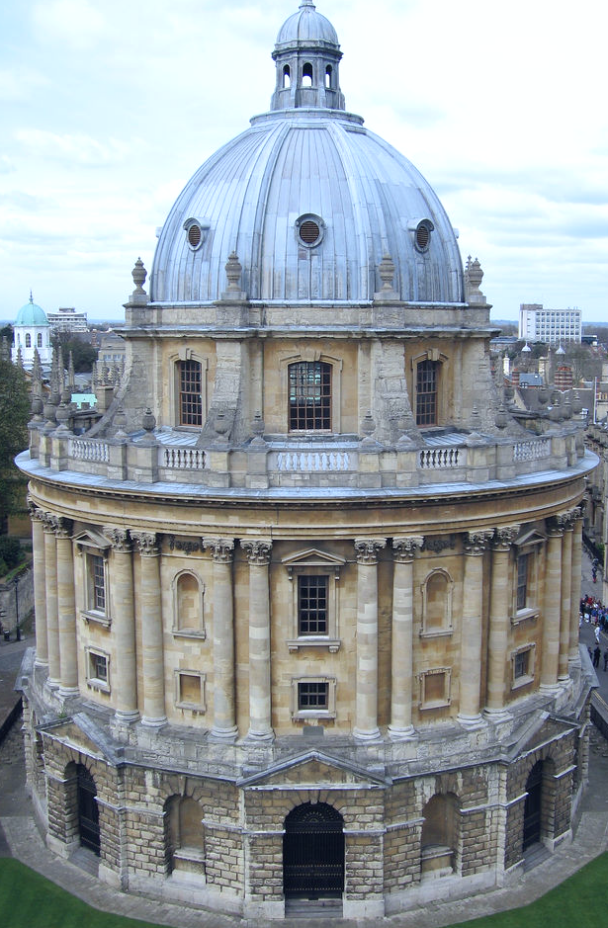
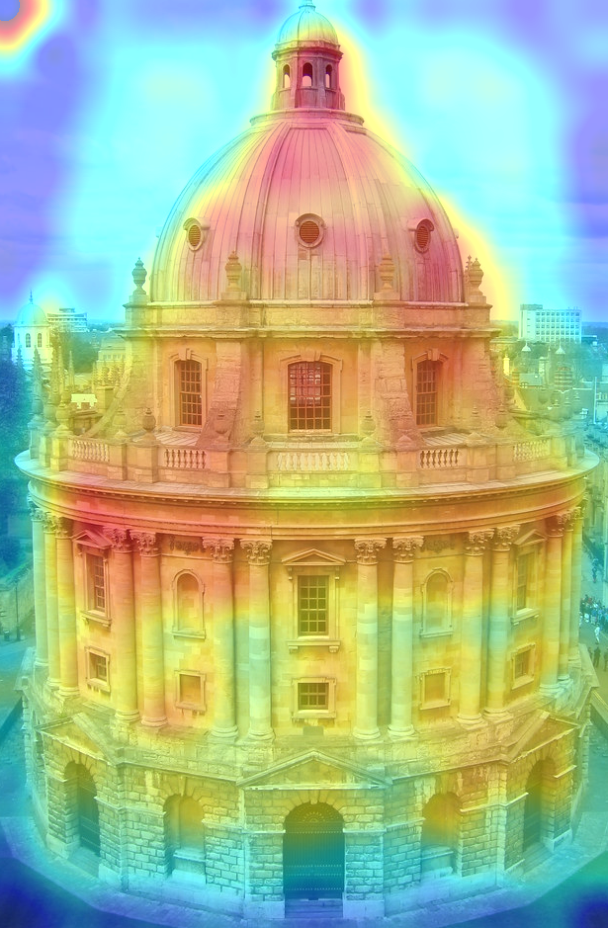
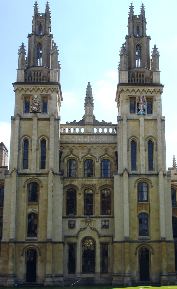
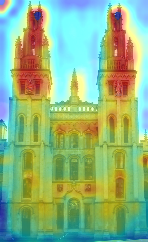
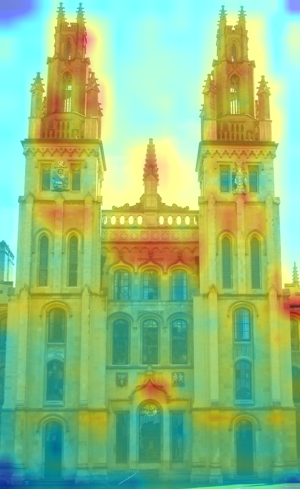
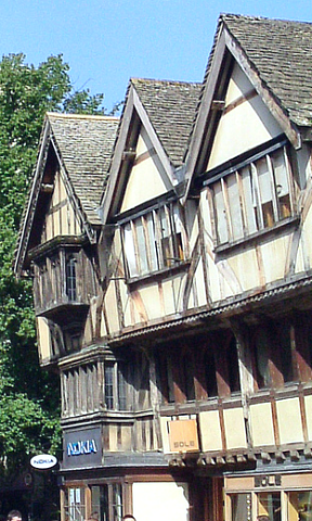
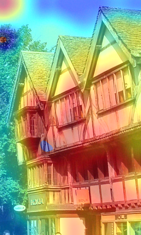
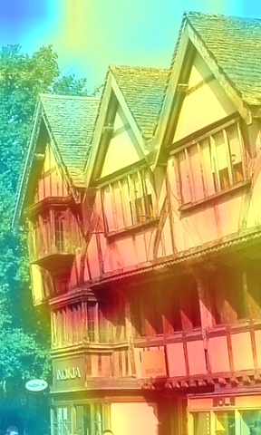
The middle column of Figure 6 shows heat maps of local spatial attention, localizing target objects in images.

Local attention feature map

We use the local channel attention map $\mathbf{A}_{c}^{l}$ to weigh $\mathbf{F}$ in the channel dimension

$$\mathbf{F}_{c}^{l}\mathrel{:=}\mathbf{F}\odot\mathbf{A}_{c}^{l}+\mathbf{F}.$$ (1)

We then use local spatial attention map $\mathbf{A}_{s}^{l}$ to weigh $\mathbf{F}_{c}^{l}$ in the spatial dimensions, resulting in the $c\times h\times w$ local attention feature map

$$\mathbf{F}^{l}=\mathbf{F}_{c}^{l}\odot\mathbf{A}_{s}^{l}+\mathbf{F}_{c}^{l}.$$ (2)

Here, $\mathbf{A}\odot\mathbf{B}$ denotes an element-wise multiplication of tensors $\mathbf{A}$ and $\mathbf{B}$, with broadcasting when one tensor is smaller. We adopt the choice of applying channel followed by spatial attention from convolutional block attention module CBAM [54]. However, apart from computing $\mathbf{A}_{s}^{l}$ at different scales, both attention maps are obtained from the original tensor $\mathbf{F}$ rather than sequentially. In addition, both (1) and (2) include residual connections, while CBAM includes a single residual connection over both steps.

Figure 4: Global channel attention.

3.2 Global attention

We extract two matrices capturing global pairwise channel and spatial interaction to weigh the feature map.

Global channel attention

We introduce a global channel attention mechanism that captures global channel interaction. This mechanism is based on the non-local neural network [52], but with the idea of 1D convolution from ECA-Net [51]. As shown in Figure 4, we are given the $c\times h\times w$ feature tensor $\mathbf{F}$ from our backbone. We apply GAP and squeeze spatial dimensions, followed by a 1D convolution of kernel size $k$ and a sigmoid function, to obtain $1\times c$ query $\mathbf{Q}_{c}$ and key $\mathbf{K}_{c}$ tensors. The value tensor $\mathbf{V}_{c}$ is obtained by mere reshaping of $\mathbf{F}$ to $hw\times c$, without GAP. Next, we form the outer product of $\mathbf{K}_{c}$ and $\mathbf{Q}_{c}$, followed by softmax over channels to obtain a $c\times c$ global channel attention map

$$\mathbf{A}_{c}^{g}=\operatorname{softmax}({\mathbf{K}_{c}}^{\top}\mathbf{Q}_{c}).$$ (3)

Finally, this attention map is multiplied with $\mathbf{V}_{c}$ and the matrix product $\mathbf{V}_{c}\mathbf{A}_{c}^{g}$ is reshaped back to $c\times h\times w$ to give the global channel attention feature map $\mathbf{G}_{c}$. In GSoP [14] and A²-Net [9], a $c\times c$ global channel attention map is obtained by multiplication of $hw\times c$ matrices; (3) is more efficient, using only an outer product of $1\times c$ vectors.

Figure 5: Global spatial attention.

Global spatial attention

Since ordinary convolution applies only a local neighborhood at a time, it cannot capture global contextual information. Thus, we apply non-local filtering [52], which is a form of self-attention [49] in the spatial dimensions. As shown in Figure 5, we are given the same $c\times h\times w$ feature tensor $\mathbf{F}$ from our backbone. By using three $1\times 1$ convolutions, which reduce channels to $c^{\prime}$, and flattening spatial dimensions to $hw$, we obtain $c^{\prime}\times hw$ query $\mathbf{Q}_{s}$, key $\mathbf{K}_{s}$, and value $\mathbf{V}_{s}$ tensors, where each column is a feature vector corresponding to a particular spatial location. We capture pairwise similarities of these vectors by matrix multiplication of $\mathbf{K}_{s}$ and $\mathbf{Q}_{s}$, followed by softmax over locations to obtain a $hw\times hw$ global spatial attention map:

$$\mathbf{A}_{s}^{g}=\operatorname{softmax}(\mathbf{K}_{s}^{\top}\mathbf{Q}_{s}).$$ (4)

This attention map is multiplied with $\mathbf{V}_{s}$ and the matrix product $\mathbf{V}_{s}\mathbf{A}_{s}^{g}$ is reshaped back to $c^{\prime}\times h\times w$ by expanding the spatial dimensions. Finally, using a ${1\times 1}$ convolution, which increases channels back to $c$, we obtain the $c\times h\times w$ global spatial attention feature map $\mathbf{G}_{s}$.

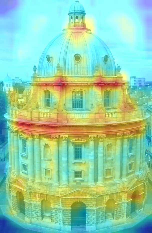
The right column of Figure 6 shows heat maps for global spatial attention, localizing target objects in images.

Global attention feature map

We use the global channel attention feature map $\mathbf{F}_{c}$ to weigh $\mathbf{F}$ element-wise

$$\mathbf{F}_{c}^{g}=\mathbf{F}\odot\mathbf{G}_{c}.$$ (5)

We then use global spatial attention feature map $\mathbf{G}_{s}$ to weigh $\mathbf{F}_{c}^{g}$ element-wise, resulting in the $c\times h\times w$ global attention feature map

$$\mathbf{F}^{g}=\mathbf{F}_{c}^{g}\odot\mathbf{G}_{s}+\mathbf{F}_{c}^{g}.$$ (6)

Similarly to $\mathbf{F}^{l}$ in (1) and (2), we apply channel attention first, followed by spatial attention. However, unlike (1), there is no residual connection in (5). This choice is supported by early experiments.

(a) input	(b) local	(c) global

Figure 6: Local and global spatial attention. Left: input images. Middle: local spatial attention heat maps. Right: global spatial attention heat maps. Red (blue) means higher (lower) attention weight.

3.3 Global-local attention

Feature fusion

As shown in Figure 1, we combine the local and global attention feature maps, $\mathbf{F}^{l}$ and $\mathbf{F}^{g}$, with the original feature $\mathbf{F}$. While concatenation and summation are common operations for feature combination, we use a weighted average with weights $w_{l}$, $w_{g}$, $w$ respectively, obtained by softmax over three learnable scalar parameters, to obtain a $c\times h\times w$ global-local attention feature map

$$\mathbf{F}^{gl}=w_{l}\mathbf{F}^{l}+w_{g}\mathbf{F}^{l}+w\mathbf{F}.$$ (7)

EfficientDet [44] has shown that this is the most effective, among a number of choices, for fusion of features across different scales.

Pooling

We apply GeM [37], a learnable spatial pooling mechanism, to feature map $\mathbf{F}^{gl}$ (7), followed by a fully-connected (FC) layer with dropout and batch normalization. The final embedding is obtained by $\ell_{2}$-normalization.

4 Experiments

Figure 7: Examples of our ranking results. In each row, the first image on the left (pink dotted outline) is a query image with a target object (red crop box), and the following are the top ranking images for the query. Orange solid outline: positive images for the query; red solid outline: negative.

4.1 Datasets

Training set

There are a number of open landmark datasets commonly used for training in image retrieval studies, including neural code (NC) [3], neural code clean (NC-clean) [16], as well as Google Landmarks v1 (GLDv1) [29] and v2 (GLDv2) [53]. Table 2 shows relevant statistics. These datasets can be categorized into noisy and clean. The clean sets were obtained from the original noisy sets for more effective training [16, 53]. The original noisy datasets are much larger, but they have high intra-class variability. Each class can include visually dissimilar images such as exterior and interior views of a building or landmark, including floor plans and paintings inside. The clean datasets focus on views directly relevant to landmark recognition but have a much smaller number of images.

Evaluation set and metrics

We use four common evaluation datasets for landmark image retrieval: Oxford5k (Ox5k) [32], Paris6k (Par6k) [33], as well as Revisited Oxford ($\mathcal{R}$Oxford or $\mathcal{R}$Oxf) and Paris ($\mathcal{R}$Paris or $\mathcal{R}$Par) [35]. $\mathcal{R}$Oxford and $\mathcal{R}$Paris are used with and without one million distractors ($\mathcal{R}$1M) [28] and evaluated using the Medium and Hard protocols [35]. We evaluate using mean Average Precision (mAP) and mean precision at 10 (mP@10).

4.2 Implementation details

We train on 8 TITAN RTX 2080Ti GPUs. All models are pre-trained on ImageNet [39] and implemented in PyTorch [31]. For fair comparisons, we set a training environment similar to the those of compared studies [56, 53, 28, 35]. We employ ResNet101 [18] as a backbone model. The kernel size $k$ of ECANet in subsection 3.1 is set to 3. The parameter $p$ of GeM in subsection 3.3 is set to 3 and the dimension $d$ of final embeddings to 512. We adopt ArcFace [10], a cosine-softmax based loss, with a margin of 0.3. We use stochastic gradient descent with initial learning rate $10^{-3}$, momentum 0.9 and weight decay $10^{-5}$.

We adopt the batch sampling of Yokoo et al. [56] where mini-batch samples with similar aspect ratios are resized to a particular size. Here, we use a batch size of 64. For image augmentation, we apply scaling, random cropping, and varied illumination. At inference, we apply a multi-resolution representation [16] to query and database images.

Our method is denoted as GLAM (global-local attention module). Using the backbone model alone is referred to as baseline. It is compatible with recent models based on ResNet101-GeM trained with ArcFace [53, 28]. Adding our local attention (subsection 3.1) to the baseline model is denoted +local, while adding our global attention (subsection 3.2) is denoted +global. Since we focus on representation learning, we do not consider post-processing methods like geometry-based re-ranking [29, 40, 53] or graph-based re-ranking [11, 21, 55].

Train Set	#Images	#Classes
NC-noisy	213,678	672
NC-clean	27,965	581
SfM-120k	117,369	713
GLDv1-noisy	1,225,029	14, 951
GLDv2-noisy	4,132,914	203,094
GLDv2-clean	1,580,470	81,313

Table 2: Statistics of different training sets.

4.3 Benchmarking

Method	Train Set	dim	Oxf5k	Par6k	$\mathcal{R}$Medium		$\mathcal{R}$Hard
					$\mathcal{R}$Oxf	$\mathcal{R}$Par	$\mathcal{R}$Oxf	$\mathcal{R}$Par
GeM-Siamese [37, 35]	SfM-120k	2048	87.8	92.7	64.7	77.2	38.5	56.3
SOLAR [28]	GLDv1-noisy	2048	–	–	69.9	81.6	47.9	64.5
GLDv2 [53]	GLDv2-clean	2048	–	–	74.2	84.9	51.6	70.3
GLAM (Ours)	NC-clean	512	77.8	85.8	51.6	68.1	20.9	44.7
	GLDv1-noisy	512	92.8	95.0	73.7	83.5	49.8	69.4
	GLDv2-noisy	512	93.3	95.3	75.7	86.0	53.1	73.8
	GLDv2-clean	512	94.2	95.6	78.6	88.5	60.2	76.8

Table 3: mAP comparison of our best model (baseline+local+global) trained on different training sets against [53, 28]. All models use ResNet101-GeM. Red: best results. Blue: GLAM higher than SOLAR [28] on GLDv1-noisy.

Method	Train Set	Dim	Base		Medium								Hard
			Ox5k	Par6k	$\mathcal{R}$Oxf		+$\mathcal{R}$1M		$\mathcal{R}$Par		+$\mathcal{R}$1M		$\mathcal{R}$Oxf		+$\mathcal{R}$1M		$\mathcal{R}$Par		+$\mathcal{R}$1M
			mAP	mAP	mAP	mP	mAP	mP	mAP	mP	mAP	mP	mAP	mP	mAP	mP	mAP	mP	mAP	mP
SPoC-V16 [2, 35]	[O]	512	53.1∗	–	38.0	54.6	17.1	33.3	59.8	93.0	30.3	83.0	11.4	20.9	0.9	2.9	32.4	69.7	7.6	30.6
SPoC-R101 [35]	[O]	2048	–	–	39.8	61.0	21.5	40.4	69.2	96.7	41.6	92.0	12.4	23.8	2.8	5.6	44.7	78.0	15.3	54.4
CroW-V16 [24, 35]	[O]	512	70.8	79.7	41.4	58.8	22.5	40.5	62.9	94.4	34.1	87.1	13.9	25.7	3.0	6.6	36.9	77.9	10.3	45.1
CroW-R101 [35]	[O]	2048	–	–	42.4	61.9	21.2	39.4	70.4	97.1	42.7	92.9	13.3	27.7	3.3	9.3	47.2	83.6	16.3	61.6
MAC-V16-Siamese [36, 35]	[O]	512	80.0	82.9	37.8	57.8	21.8	39.7	59.2	93.3	33.6	87.1	14.6	27.0	7.4	11.9	35.9	78.4	13.2	54.7
MAC-R101-Siamese [35]	[O]	2048	–	–	41.7	65.0	24.2	43.7	66.2	96.4	40.8	93.0	18.0	32.9	5.7	14.4	44.1	86.3	18.2	67.7
RMAC-V16-Siamese [36, 35]	[O]	512	80.1	85.0	42.5	62.8	21.7	40.3	66.2	95.4	39.9	88.9	12.0	26.1	1.7	5.8	40.9	77.1	14.8	54.0
RMAC-R101-Siamese [35]	[O]	2048	–	–	49.8	68.9	29.2	48.9	74.0	97.7	49.3	93.7	18.5	32.2	4.5	13.0	52.1	87.1	21.3	67.4
RMAC-R101-Triplet [16, 35]	NC-clean	2048	86.1	94.5	60.9	78.1	39.3	62.1	78.9	96.9	54.8	93.9	32.4	50.0	12.5	24.9	59.4	86.1	28.0	70.0
GeM-R101-Siamese [37, 35]	SfM-120k	2048	87.8	92.7	64.7	84.7	45.2	71.7	77.2	98.1	52.3	95.3	38.5	53.0	19.9	34.9	56.3	89.1	24.7	73.3
AGeM-R101-Siamese [17]	SfM-120k	2048	–	–	67.0	–	–	–	78.1	–	–	–	40.7	–	–	–	57.3	–	–	–
SOLAR-GeM-R101-Triplet/SOS [28]	GLDv1-noisy	2048	–	–	69.9	86.7	53.5	76.7	81.6	97.1	59.2	94.9	47.9	63.0	29.9	48.9	64.5	93.0	33.4	81.6
DELG-GeM-R101-ArcFace [5]	GLDv1-noisy	2048	–	–	73.2	–	54.8	–	82.4	–	61.8	–	51.2	–	30.3	–	64.7	–	35.5	–
GeM-R101-ArcFace [53]	GLDv2-clean	2048	–	–	74.2	–	–	–	84.9	–	–	–	51.6	–	–	–	70.3	–	–	–
GLAM-GeM-R101-ArcFace baseline	GLDv2-clean	512	91.9	94.5	72.8	86.7	58.1	78.2	84.2	95.9	63.9	93.3	49.9	62.1	31.6	49.7	69.7	88.4	37.7	73.7
+local	GLDv2-clean	512	91.2	95.4	73.7	86.2	60.5	77.4	86.5	95.6	68.0	93.9	52.6	65.3	36.1	55.6	73.7	89.3	44.7	79.1
+global	GLDv2-clean	512	92.3	95.3	77.2	87.0	63.8	79.3	86.7	95.4	67.8	93.7	57.4	69.6	38.7	57.9	75.0	89.4	45.0	77.0
+global+local	GLDv2-clean	512	94.2	95.6	78.6	88.2	68.0	82.4	88.5	97.0	73.5	94.9	60.2	72.9	43.5	62.1	76.8	93.4	53.1	84.0

Table 4: mAP comparison of our GLAM against SOTA methods based on global descriptors without re-ranking. V16: VGG16; R101: ResNet101. [O]: Off-the-shelf (pre-trained on ImageNet). ^∗: dimension $d=256$ [2]. mP: mP@10. Red: best results. Black bold: best previous methods. Blue: GLAM higher than previous methods. Weyand et al. [53] is the only model other than ours trained on GLDv2-clean, while [28] is trained on GLDv1-noisy and compared in Table 3.

Noisy vs. clean training sets

We begin by training our best model (baseline+local+global) on all training sets of Table 2, except NC-noisy because some images are currently unavailable. As shown in Table 3, even though GLDv2-noisy has 2.6 times more images than GLDv2-clean, the latter is superior by a large margin. This shows that, in training, a cleaner dataset can be more important than a larger one. By contrast, NC-clean has the worst performance despite being clean, aparently because it is too small. To achieve best possible performance, we use GLDv2-clean as a training set in the remaining experiments.

Comparisons on same training set

It is common to compare methods regardless of training sets as more become available, e.g., [35, 28]. Since GLDv2-clean is relatively new, Weyand et al. [53], which introduced the dataset, is the only study that has trained the same backbone with the same settings (ResNet101-GeM with ArcFace) on GLDv2-clean. Our baseline is lower than [53], because our dimensinality is 512, while other models based on ResNet101 use 2048. Yet, Table 3 shows that our best model trained on GLDv2-clean outperforms [53] by a large margin. But the most important comparison is with SOLAR [28], also based on self-attention, which has trained ResNet101-GeM on GLDv1-noisy. On this training set, our best model clearly outperforms [28] despite lower dimensionality.

Comparison with state of the art

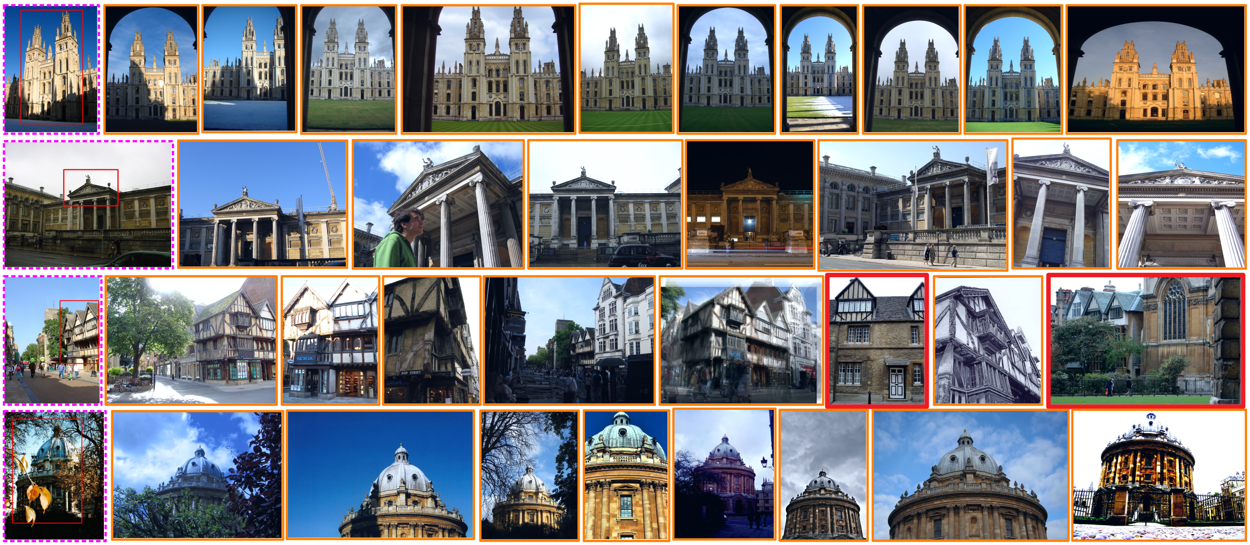
Table 4 shows the performance of four variants of our model, i.e. baseline with or without local/global attention, and compares them against state-of-the-art (SOTA) methods based on global descriptors without re-ranking on the complete set of benchmarks, including distractors. Both local and global attention bring significant gain over the baseline. The effect of global is stronger, while the gain of the two is additive in the combination. The best results are achieved by the global-local attention network (baseline+global+local). With this model, we outperform previous best methods on most benchmarks except mP@10 on $\mathcal{R}$Paris (medium) and $\mathcal{R}$Paris$+$$\mathcal{R}$1M (medium), where we are outperformed by [37, 35]. These results demonstrate that our approach is effective for landmark image retrieval. Figure 7 shows some examples of our ranking results.

4.4 Ablation study

Method	Oxf5k	Par6k	$\mathcal{R}$Medium		$\mathcal{R}$Hard
			$\mathcal{R}$Oxf	$\mathcal{R}$Par	$\mathcal{R}$Oxf	$\mathcal{R}$Par
GLAM baseline	91.9	94.5	72.8	84.2	49.9	69.7
+local-channel	91.3	95.3	72.2	85.8	48.3	73.1
+local-spatial	91.0	95.1	72.1	85.3	48.3	71.9
+local	91.2	95.4	73.7	86.5	52.6	75.0
+global-channel	92.5	94.4	73.3	84.4	49.8	70.1
+global-spatial	92.4	95.1	73.2	86.3	50.0	72.7
+global	92.3	95.3	77.2	86.7	57.4	75.0
+global+local	94.2	95.6	78.6	88.5	60.2	76.8

Table 5: mAP comparison of spatial and channel variants of our local (+local, subsection 3.1) and global (+global, subsection 3.1) attention modules to the baseline.

Method	Oxf5k	Par6k	$\mathcal{R}$Medium		$\mathcal{R}$Hard
			$\mathcal{R}$Oxf	$\mathcal{R}$Par	$\mathcal{R}$Oxf	$\mathcal{R}$Par
CBAM style	93.8	95.7	75.6	88.4	53.3	76.8
GLAM (Ours)	94.2	95.6	78.6	88.5	60.2	76.8

Table 6: mAP comparison between CBAM style and our local spatial attention.

Method	Oxf5k	Par6k	$\mathcal{R}$Medium		$\mathcal{R}$Hard
			$\mathcal{R}$Oxf	$\mathcal{R}$Par	$\mathcal{R}$Oxf	$\mathcal{R}$Par
Concatenate	89.5	95.1	73.6	86.5	54.0	73.7
Sum (Ours)	94.2	95.6	78.6	88.5	60.2	76.8

Table 7: mAP comparison between weighted concatenation and weighted average for feature fusion.

Method	Oxf5k	Par6k	$\mathcal{R}$Medium		$\mathcal{R}$Hard
			$\mathcal{R}$Oxf	$\mathcal{R}$Par	$\mathcal{R}$Oxf	$\mathcal{R}$Par
Fixed-size	76.1	82.6	55.7	68.4	29.2	47.5
Group-size (Ours)	94.2	95.6	78.6	88.5	60.2	76.8

Table 8: mAP comparison between fixed-size ($224\times 224$) and group-size sampling methods.

Query	Database	Oxf5k	Par6k	$\mathcal{R}$Medium		$\mathcal{R}$Hard
				$\mathcal{R}$Oxf	$\mathcal{R}$Par	$\mathcal{R}$Oxf	$\mathcal{R}$Par
Single	Single	93.3	95.2	76.9	87.1	58.6	74.7
Multi	Single	93.9	95.4	78.0	87.7	59.0	75.5
Single	Multi	93.6	95.6	77.0	87.8	57.1	76.0
Multi	Multi	94.2	95.6	78.6	88.5	60.2	76.8

Table 9: mAP comparison of using multiresolution representation (Multi) or not (Single) on query or database.

Our ablation study uses the Google Landmark v2 clean dataset (GLDv2-clean) [53] for training, which is shown to be the most effective in Table 3.

Effect of attention modules

We ablate the effect of our local and global attention networks as well as their combination. Table 5 shows the results, which are more fine-grained than those of Table 4. In particular, it shows the effect of the channel and spatial variants of both local and global attention. We observe that, when used alone, the channel and spatial variants of local attention are harmful in most cases. Even the combination, baseline+local, is not always effective. By contrast, when used alone, the channel and spatial variants of global attention are mostly beneficial, especially the latter. Their combination, baseline+global, is impressive, bringing gain of up to 7.5%. Importantly, the combination baseline+global+local improves further by up to another 2.8%. This result shows the necessity of local attention in the final model.

CBAM vs. our local spatial attention

We experiment with the local spatial attention of CBAM [54]. CBAM applies average and max-pooling to input features and concatenates the two for spatial attention. We apply this variant to our local spatial attention module for comparison. For the CBAM style module, we keep the overall design of our module as shown in Figure 3, but apply average and max-pooling to each of the four convolutional layer outputs before concatenation. Table 6 shows that the CBAM style module is considerably worse than ours on all benchmarks except Paris6k, where it is only slightly better.

Concatenation vs. sum for feature fusion

We use a softmax-based weighted average of local and global attention feature maps with the original feature map (7). Here, we compare this weighted average with weighted concatenation, where concatenation replaces the sum operation in (7). As shown in Table 7, the weighted average outperforms the weighted concatenation.

Fixed-size vs. group-size sampling

Numerous studies have proposed methods for constructing batches according to image size for efficient training. For instance, Gordo et al. [16], DELF [29], and Yokoo et al. [56] employed different image sizes per batch for training instead of a single fixed size. We adopt the method of Yokoo et al., which constructs a batch with images of similar aspect ratio, so that the images can be resized to a size with an aspect ratio that is similar to their own. We call this method group-size sampling. Table 8 compares fixed-size ($224\times 224$) with group-size sampling. We observe that maintaining aspect ratios by using dynamic input sizes is much more effective.

Multi-resolution

We use the multi-resolution representation [16] for the final feature of an image at inference time. This method: (1) resizes an image into multiple scales; (2) extracts features from the resized images; and (3) averages the features to obtain the final feature of the image. The method is applied to both query and database images to enhance ranking results, especially for small target objects. Table 9 compares the four cases of applying this method or not to query or database images.

5 Conclusion

We have introduced a novel approach that extracts global and local contextual information using attention mechanisms for instance-level image retrieval. It is manifested as a network architecture consisting of global and local attention components, each operating on both spatial and channel dimensions. This constitutes a comprehensive study and empirical evaluation of all four forms of attention that have previously been studied only in isolation. Our findings indicate that the gain (or loss) brought by one form of attention alone strongly depends on the presence of the others, with the maximum gain appearing when all forms are present. The output is a modified feature tensor that can be used in any way, for instance with local feature detection instead of spatial pooling for image retrieval.

With the advent of vision transformers [12, 58] and their recent application to image retrieval [13], attention is expected to play a more and more significant role in vision. According to our classification, transformers perform global spatial attention alone. It is of great interest to investigate the role of the other forms of attention, where our approach may yield a basic building block of such architectures. One may even envision an extension to language models, where transformers originate from [50].

References

- [1] Relja Arandjelović, Petr Gronat, Akihiko Torii, Tomas Pajdla, and Josef Sivic. NetVLAD: CNN architecture for weakly supervised place recognition. In CVPR, 2016.
- [2] Artem Babenko and Victor Lempitsky. Aggregating Local Deep Features for Image Retrieval. In ICCV, 2015.
- [3] Artem Babenko, Anton Slesarev, Alexandr Chigorin, and Victor Lempitsky. Neural Codes for Image Retrieval. In ECCV, 2014.
- [4] Irwan Bello, Barret Zoph, Ashish Vaswani, Jonathon Shlens, and Quoc V. Le. Attention augmented convolutional networks. In ICCV, 2019.
- [5] Bingyi Cao, André Araujo, and Jack Sim. Unifying deep local and global features for image search. In ECCV, 2020.
- [6] Yue Cao, Jiarui Xu, Stephen Lin, Fangyun Wei, and Han Hu. GCNet: Non-Local Networks Meet Squeeze-Excitation Networks and Beyond. In ICCV, 2019.
- [7] Liang-Chieh Chen, George Papandreou, Florian Schroff, and Hartwig Adam. Rethinking atrous convolution for semantic image segmentation. arXiv preprint arXiv:1706.05587, 2017.
- [8] Ting Chen, Simon Kornblith, Mohammad Norouzi, and Geoffrey Hinton. A simple framework for contrastive learning of visual representations. In ICML, 2020.
- [9] Yunpeng Chen, Yannis Kalantidis, Jianshu Li, Shuicheng Yan, and Jiashi Feng. A^2-nets: Double attention networks. In NeurIPS, 2018.
- [10] Jiankang Deng, Jia Guo, Niannan Xue, and Stefanos Zafeiriou. ArcFace: Additive Angular Margin Loss for Deep Face Recognition. In CVPR, 2019.
- [11] Michael Donoser and Horst Bischof. Diffusion Processes for Retrieval Revisited. In CVPR, 2013.
- [12] Alexey Dosovitskiy, Lucas Beyer, Alexander Kolesnikov, Dirk Weissenborn, Xiaohua Zhai, Thomas Unterthiner, Mostafa Dehghani, Matthias Minderer, Georg Heigold, Sylvain Gelly, et al. An image is worth 16x16 words: Transformers for image recognition at scale. arXiv preprint arXiv:2010.11929, 2020.
- [13] Alaaeldin El-Nouby, Natalia Neverova, Ivan Laptev, and Hervé Jégou. Training vision transformers for image retrieval. Technical report, 2021.
- [14] Zilin Gao, Jiangtao Xie, Qilong Wang, and Peihua Li. Global second-order pooling convolutional networks. In CVPR, 2019.
- [15] Albert Gordo, Jon Almazan, Jerome Revaud, and Diane Larlus. Deep image retrieval: Learning global representations for image search. In ECCV, 2016.
- [16] Albert Gordo, Jon Almazan, Jerome Revaud, and Diane Larlus. End-to-end learning of deep visual representations for image retrieval. IJCV, 2017.
- [17] Yinzheng Gu, Chuanpeng Li, and Jinbin Xie. Attention-aware generalized mean pooling for image retrieval. arXiv preprint arXiv:1811.00202, 2018.
- [18] Kaiming He, Xiangyu Zhang, Shaoqing Ren, and Jian Sun. Deep residual learning for image recognition. In CVPR, 2016.
- [19] Jie Hu, Li Shen, Samuel Albanie, Gang Sun, and Andrea Vedaldi. Gather-excite: Exploiting feature context in convolutional neural networks. In NeurIPS, 2018.
- [20] Jie Hu, Li Shen, Samuel Albanie, Gang Sun, and Enhua Wu. Squeeze-and-Excitation Networks. In CVPR, 2018.
- [21] Ahmet Iscen, Giorgos Tolias, Yannis Avrithis, Teddy Furon, and Ondrej Chum. Efficient diffusion on region manifolds: Recovering small objects with compact cnn representations. In CVPR, 2017.
- [22] H. Jegou, F. Perronnin, M. Douze, J. Sanchez, P. Perez, and C. Schmid. Aggregating local image descriptors into compact codes. PAMI, (99):1–1, 2011.
- [23] Albert Jimenez, Jose M. Alvarez, and Xavier Giró-i-Nieto. Class weighted convolutional features for visual instance search. In BMVC, 2017.
- [24] Yannis Kalantidis, Clayton Mellina, and Simon Osindero. Crossdimensional weighting for aggregated deep convolutional features. In ECCV, 2016.
- [25] Hyo Jin Kim, Enrique Dunn, and Jan-Michael Frahm. Learned Contextual Feature Reweighting for Image Geo-Localization. In CVPR, 2017.
- [26] Sungyeon Kim, Dongwon Kim, Minsu Cho, and Suha Kwak. Proxy anchor loss for deep metric learning. In CVPR, 2020.
- [27] David G. Lowe. Distinctive image features from scale-invariant keypoints. In IJCV, 2004.
- [28] Tony Ng, Vassileios Balntas, Yurun Tian, and Krystian Mikolajczyk. SOLAR: Second-Order Loss and Attention for Image Retrieval. In ECCV, 2020.
- [29] Hyeonwoo Noh, Andre Araujo, Jack Sim, Tobias Weyand, and Bohyung Han. Large Scale Image Retrieval with Attentive Deep Local Features. In ICCV, 2017.
- [30] Hyun Oh Song, Yu Xiang, Stefanie Jegelka, and Silvio Savarese. Deep metric learning via lifted structured feature embedding. In CVPR, 2016.
- [31] Adam Paszke, Sam Gross, Francisco Massa, Adam Lerer, James Bradbury, Gregory Chanan, Trevor Killeen, Zeming Lin, Natalia Gimelshein, Luca Antiga, Alban Desmaison, Andreas Köpf, Edward Yang, Zach DeVito, Martin Raison, Alykhan Tejani, Sasank Chilamkurthy, Benoit Steiner, Lu Fang, Junjie Bai, and Soumith Chintala. PyTorch: An imperative style, high-performance deep learning. In NeurIPS, 2019.
- [32] James Philbin, Ondrej Chum, Michael Isard, Josef Sivic, and Andrew Zisserman. Object retrieval with large vocabularies and fast spatial matching. In CVPR, 2007.
- [33] James Philbin, Ondrej Chum, Michael Isard, Josef Sivic, and Andrew Zisserman. Lost in quantization:Improving particular object retrieval in large scale image databases. In CVPR, 2008.
- [34] Tobias Plötz and Stefan Roth. Neural nearest neighbors networks. In NeurIPS, 2018.
- [35] Filip Radenović, Ahmet Iscen, Giorgos Tolias, Yannis Avrithis, and Ondřej Chum. Revisiting Oxford and Paris: Large-Scale Image Retrieval Benchmarking. In CVPR, 2018.
- [36] Filip Radenović, Giorgos Tolias, and Ondřej Chum. CNN image retrieval learns from BoW: Unsupervised fine-tuning with hard examples. In ECCV, 2016.
- [37] Filip Radenović, Giorgos Tolias, and Ondřej Chum. Fine-Tuning CNN Image Retrieval with No Human Annotation. In TPAMI, 2019.
- [38] Ali Sharif Razavian, Josephine Sullivan, Stefan Carlsson, and Atsuto Maki. Visual Instance Retrieval with Deep Convolutional Networks. In CoRR, 2015.
- [39] Olga Russakovsky, Jia Deng, Hao Su, Jonathan Krause, Sanjeev Satheesh, Sean Ma, Zhiheng Huang, Andrej Karpathy, Aditya Khosla, Michael Bernstein, Alexander C. Berg, and Li Fei-Fei. ImageNet Large Scale Visual Recognition Challenge. In International booktitle of Computer Vision, 2015.
- [40] Oriane Siméoni, Yannis Avrithis, and Ondrej Chum. Local features and visual words emerge in activations. In CVPR, 2019.
- [41] O. Siméoni, A. Iscen, G. Tolias, Y. Avrithis, and O. Chum. Graph-based particular object discovery. Machine Vision and Applications, 30(2):243–254, 3 2019.
- [42] Jake Snell, Kevin Swersky, and Richard S. Zemel. Prototypical networks for few-shot learning. In NeurIPS, 2017.
- [43] Christian Szegedy, Wei Liu, Yangqing Jia, Pierre Sermanet, Scott Reed, Dragomir Anguelov, Dumitru Erhan, Vincent Vanhoucke, and Andrew Rabinovich. Going deeper with convolutions. In CVPR, 2015.
- [44] Mingxing Tan, Ruoming Pang, and Quoc V. Le. EfficientDet: Scalable and Efficient Object Detection. In CVPR, 2020.
- [45] Marvin Teichmann, Andre Araujo, Menglong Zhu, and Jack Sim. Detect-to-retrieve: Efficient regional aggregation for image search. In CVPR, 2019.
- [46] Giorgios Tolias, Yannis Avrithis, and Hervé Jégou. To aggregate or not to aggregate: Selective match kernels for image search. In ICCV, 2013.
- [47] Giorgos Tolias, Tomas Jenicek, and Ondřej Chum. Learning and aggregating deep local descriptors for instance-level recognition. In ECCV, 2020.
- [48] Giorgos Tolias, Ronan Sicre, and Hervé Jégou. Particular object retrieval with integral max-pooling of CNN activations. In ICLR, 2016.
- [49] Ashish Vaswani, Noam Shazeer, Niki Parmar, Jakob Uszkoreit, Llion Jones, Aidan N. Gomez, Lukasz Kaiser, and Illia Polosukhin. Attention is all you need. In NeurIPS, 2017.
- [50] Ashish Vaswani, Noam Shazeer, Niki Parmar, Jakob Uszkoreit, Llion Jones, Aidan N Gomez, Lukasz Kaiser, and Illia Polosukhin. Attention is all you need. In NeurIPS, 2017.
- [51] Qilong Wang, Banggu Wu, Pengfei Zhu, Peihua Li, Wangmeng Zuo, and Qinghua Hu. ECA-Net: Efficient Channel Attention for Deep Convolutional Neural Networks. In CVPR, 2020.
- [52] Xiaolong Wang, Ross Girshick, Abhinav Gupta, and Kaiming He. Non-local Neural Networks. In CVPR, 2018.
- [53] Tobias Weyand, Andre Araujo, Bingyi Cao, and Jack Sim. Google Landmarks Dataset v2 - A Large-Scale Benchmark for Instance-Level Recognition and Retrieval. In CVPR, 2020.
- [54] Sanghyun Woo, Jongchan Park, Joon-Young Lee, and In So Kweon. CBAM: Convolutional Block Attention Module. In ECCV, 2018.
- [55] Fan Yang, Ryota Hinami, Yusuke Matsui, Steven Ly, and Shin’ichi Satoh. Efficient image retrieval via decoupling diffusion into online and offline processing. In AAAI, 2019.
- [56] Shuhei Yokoo, Kohei Ozaki, Edgar Simo-Serra, and Satoshi Iizuka. Two-stage Discriminative Re-ranking for Large-scale Landmark Retrieval. In arXiv:2003.11211, 2020.
- [57] Fisher Yu, Vladlen Koltun, and Thomas Funkhouser. Dilated residual networks. In CVPR, 2017.
- [58] Li Yuan, Yunpeng Chen, Tao Wang, Weihao Yu, Yujun Shi, Francis EH Tay, Jiashi Feng, and Shuicheng Yan. Tokens-to-token vit: Training vision transformers from scratch on imagenet. arXiv preprint arXiv:2101.11986, 2021.
- [59] Hengshuang Zhao, Jiaya Jia, and Vladlen Koltun. Exploring self-attention for image recognition. In CVPR, 2020.