11email: hliang2@andrew.cmu.edu, lulany@alumni.cmu.edu, guikangx@alumni.cmu.edu, {bhiksha, rsingh}@cs.cmu.edu
Controlled AutoEncoders to Generate Faces from Voices
Abstract
Multiple studies in the past have shown that there is a strong correlation between human vocal characteristics and facial features. However, existing approaches generate faces simply from voice, without exploring the set of features that contribute to these observed correlations. A computational methodology to explore this can be devised by rephrasing the question to: “how much would a target face have to change in order to be perceived as the originator of a source voice?” With this in perspective, we propose a framework to morph a target face in response to a given voice in a way that facial features are implicitly guided by learned voice-face correlation in this paper. Our framework includes a guided autoencoder that converts one face to another, controlled by a unique model-conditioning component called a gating controller which modifies the reconstructed face based on input voice recordings. We evaluate the framework on VoxCelab and VGGFace datasets through human subjects and face retrieval. Various experiments demonstrate the effectiveness of our proposed model.
Index Terms: controlled autoencoder, face generation, speech-face association learning, voice-face biometric matching
1 Introduction
Curiosity has long driven humans to picture what someone else looks like upon hearing his/her voice. One of the assumptions, presumably made based on millennia of experience, is that there exists a statistical relation between what a person looks like, and what they sound like [1]. Some of these relations are immediately obvious, e.g. we expect the visage that goes with old-sounding voices to look old, and that of female voices to be female. Besides these obvious covariates, however, it may be expected that there are other unapparent dependencies between human vocal characteristics and facial features, since humans are able to associate faces with voices with surprising accuracy [2].
In trying to visualize the face behind a voice, however, we do not generally begin de novo, drawing up the face from whole cloth. Indeed, if one were to try to imagine the source of a sound such as voice with no prior information at all, it is highly unlikely that one would picture anything resembling a face. Therefore, we visualize faces based on two hypotheses:
-
•
First, that in identifying the sound as a human voice, we draw upon the general shape of human faces, rather than any physical object that could produce the sound, and
-
•
Second, that we draw upon an actual imagined face and make the modifications we deem necessary to match the voice.
The problem of automatically guessing speakers’ faces from voice recordings has recently gained some popularity (or notereity, depending on the reader’s perspective) [3, 4, 5]. The proposed approaches have taken two paths. The first, “matching” approach finds the most suitable face from a collection [6, 7], which is fundamentally restricted by the selection of faces it can choose from and cannot generate entirely novel faces. The second, “generation” approach attempts to synthesize the facial image [3]. The approach embodies the first of our two hypotheses above : the proposed solutions learn a generic statistical model for the relationship between voices and face-like images, which they use to generate faces from novel voices. However, learning such statistical models is fraught with challenge. As [8] discover, direct modelling of statistical dependencies can result in models that often do not generate images that are even facelike. More sophisticated approaches do manage to generate face-like imagery, but these often show distortions [9, 10]. While one may nevertheless try to produce better-quality visualizations, these techniques are dependent more on the well-known ability of GANs and similar models to hallucinate near-perfect faces [11, 10], than on any dependence of these faces on all but the highest-level aspects of the voice, such as gender and age. Even so, they will still suffer problems such as mode collapse (whereby all voices end up producing the same face)[3, 12], and lack of variety in the generated faces [11].
In this paper we take a different approach based on the second of our hypotheses above: that it may be easier to generate realistic facsimiles of a speaker’s face if one were to begin with an initial template of an actual face and only make the minimal changes necessary to it (retaining as many features from the input face as possible), to make it match the voice. Accordingly, we propose a new model that begins with an initial “proposal” face image, and makes adjustments to it according to information extracted from the voice.
Our proposed model, which we will refer to as a controlled AutoEncoder (CAE), comprises two components. The primary component is a scaffolding based on a U-net-like [13] autoencoder, which takes in the proposal face and outputs a redrawn face. In the absence of other signals, the network must regenerate the input proposal face. The second component, which accepts the voice input, is a gating controller that modifies the parameters of the decoder based on information derived from the voice, to modify the generated face to match the voice. While being trained, the model also includes a discriminative component that is used to optimize the parameters of the network. The entire model is learned using a set of losses that simultaneously capture the degree of match to the target (speaker’s) face and deviation from the proposal face. The CAE has several advantages over prior models. Being fundamentally an autoencoder, the output does not diverge from a face. As a morphing mechanism, rather than a genreating one, it does not face problems such as mode collapse. Diversity of output may be obtained simply by changing the proposal face.
Experimental results show that our model performs well under several evaluation metrics, including human subjective evaluation, feature similarity and face retrieval performance.
2 The controlled AutoEncoder model
The purpose of our model is to modify an input “proposal” face image to best match a given voice. The model has two components: an autoencoder based on a U-net-like [13] structure that derives a latent representation of the proposal face and attempts to reconstruct the latter from it, and a gating controller that modifies the parameters of the decoder based on the input speech signal. We describe the two below.
2.1 The AutoEncoder scaffold
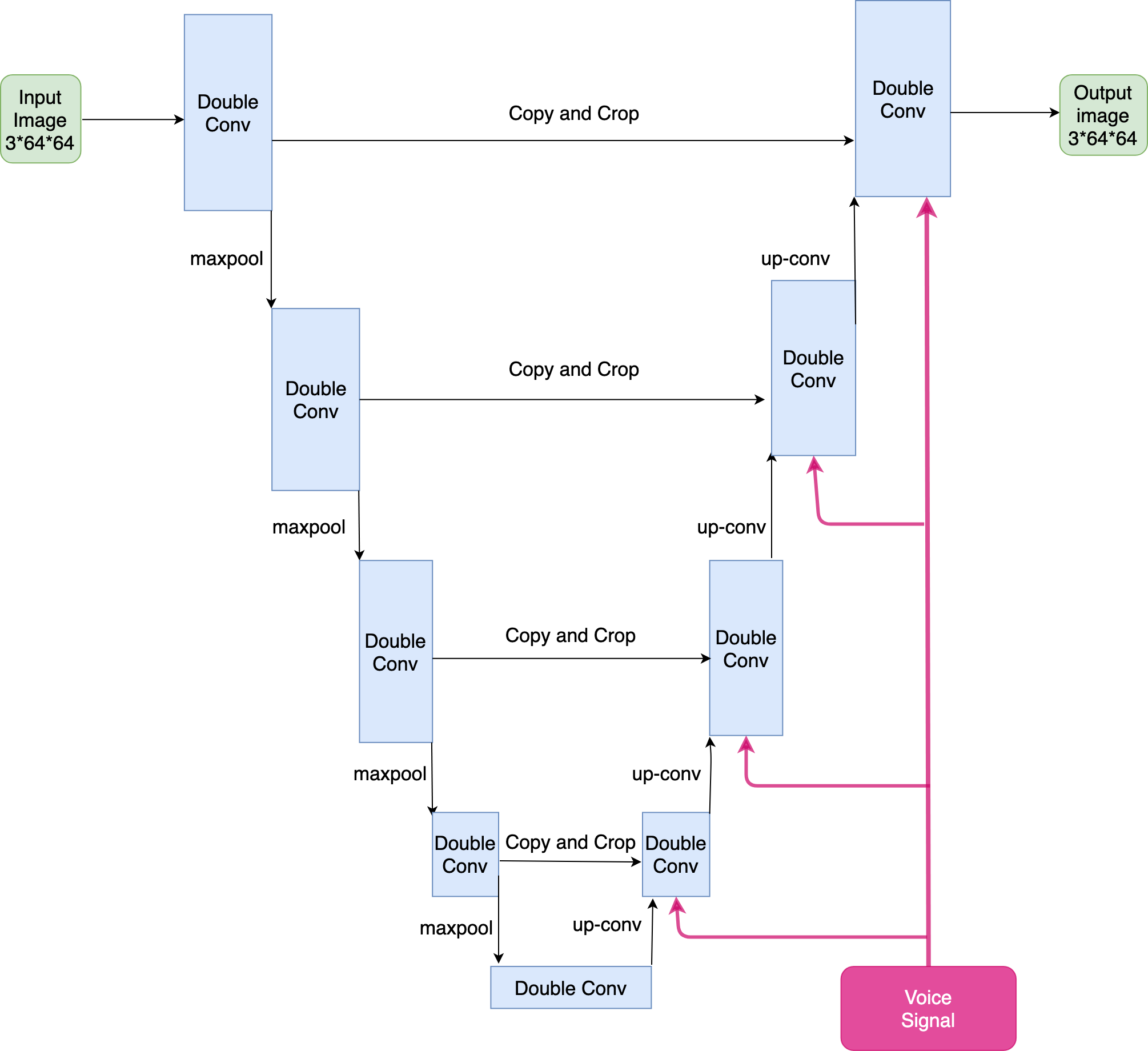
The main scaffold of our model is an autoencoder that derives a latent representation from the proposal face and reconstructs it from this representation. We specifically choose the U-net structure [13] for reasons we will shortly explain. The U-net includes an encoder that comprises a sequence of downsampling convolutional layers, ending finally in a simple, low-dimensional representation of the input image. This is followed by a decoder that comprises a sequence of upsampling transpose-convolutional layers that recreate the input image from the latent representation. The structure of the entire network is symmetric around its central latent-representation layer – corresponding to each layer of the encoder is a complementary decoder layer that is at an identical distance (or depth) from the central latent-representation layer, and has the same size as its encoder complement.
What distinguishes the U-net from conventional autoencoders is that the U-net also includes direct “skip” connections from each encoder layer to its complementary decoder layer. This is particularly relevant to our model, since it provides a pathway for information about the details of the face to be retained, while permitting high-level latent characteristics to be modified.
The blue components of Figure 1 illustrate the U-net AE scaffolding of our model.
In our implementation the encoder consists of 4 convolutional layers with 64,128,256 and 512 output channels. All convolutional filters are size . Convolutional layers followed by maxpooling layers of size , with stride 2. The decoder is the mirror image of the encoder, sans the pooling layers. The transpose convolution in the decoder has a stride of size 2. Input images are rescaled to and output images too are the same size.
2.2 The gating controller
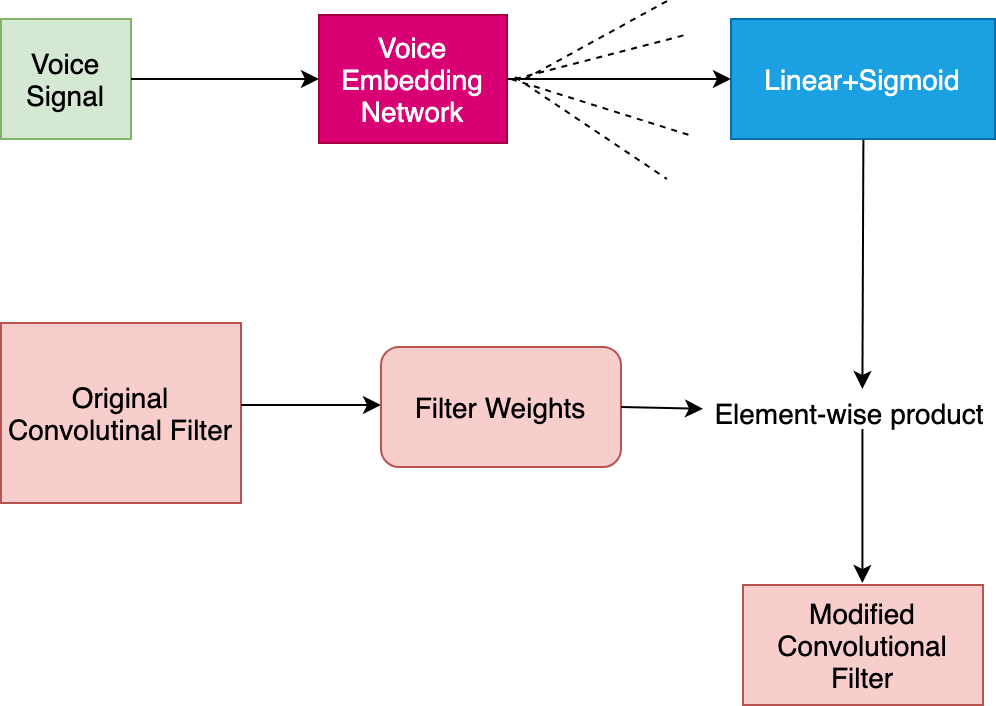
The gating controller modifies the trasverse convolutional filters of the decoder, based on the voice signal.
In our setup, the voice recordings, duly endpointed, are first transformed into a 64-dimensional log mel-spectrographic representation, computed using an analysis window of 25ms and a frameshift of 10ms. The resulting spectrographic representation is fed to an embedding network, which produces a 64-dimensional embedding of the voice signal. The voice embedding is subsequently input, in parallel, to a number of linear layers, one each corresponding to each layer of the decoder. The linear layer corresponding to each decoder layer produces as many outputs as the number of convolutional filter parameters in the decoder layer. The outputs of the linear layer are passed through a sigmoid activation. The outputs of the sigmoid multiply the parameters of the filters, thereby modifying them.
The pink components of Figure 1 illustrate the overall operation of the gating controller. Figure 2 shows the details of the gating control for one of the decoder layers. The dotted lines in the figure show paths to other layers.
The embedding network is a key component of this framework, as it is intended to extract speaker-specific information from the voice. For our work we employ an architecture derived from [10], where it was found to be effective for biometric voice-to-face matching. Table 1 shows the architecture of the embedding network. It too is a convolutional network etc. are the lengths (temporal) of the the input after each layer, which compresses the input length with a stride of 2. We found it most effective to pre-train the voice embedding network, using the DimNet framework from [10], and to subsequently fix the network.
| Voice Embedding Network | ||
|---|---|---|
| Layer | Act. | Output shape |
| Input | - | |
| Conv | BN+ReLU | |
| Conv | BN+ReLU | |
| Conv | BN+ReLU | |
| Conv | BN+ReLU | |
| Conv | BN+ReLU | |
| AvgPool | - | |
| Discriminator/Classifier | ||
|---|---|---|
| Layer | Act. | Output shape |
| Input | - | |
| Conv | LReLU | |
| Conv . | LReLU | |
| Conv | LReLU | |
| Conv | LReLU | |
| Conv | LReLU | |
| Conv | LReLU | |
3 Training and inference
3.1 Training the network
The network is trained on a collection of training instances, where each instance comprises an original face, a target voice and the corresponding target face. We optimize the parameters of the network to try to ensure that the output of the U-net stays close to its input, while simultaneously capturing the identity of the speaker. To support this, during the learning phase, we include two additional components, that work on the image produced by the model:
-
•
A binary discriminator that is intended to ensure that the generated images are facelike. The architecture for which is also described in Table 1.
-
•
A multi-class classifier which tries to enforce the visual identity of the speaker on the generated face. The classifier is a shared structure with the discriminator, with the exception that the final representation layer of the discriminator forks off into a multi-class softmax layer with as many outputs as we have subjects in the training data.
We employ a number of losses to train the network. We explain these below. In the explanation we represent real faces with f, synthetic faces with , voice with v, and identity label with I. In terms of model components, we use to represent the generator (the scaffolding), for the discriminator, and for classifier.
-
•
L1-norm loss: (,) computes the total norm of the error between the RGB values of two face images and .
-
•
Classifier loss: (f,I) is the cross-entropy between the classifier’s output and a one-hot representation of the identity of the speaker.
-
•
Discriminator loss: (f,I) computes a binary cross entropy between the discriminator output and a binary label that specifies if the image input to the discriminator is synthetic or real.
The actual training paradigm, which is inspired by [6, 10], StarGAN [14] and CycleGAN [15], tries to simultaneously satisfy multiple objectives.
First, the output of the generator must be similar to the target face, i.e. , where denotes the face image of original identity and denotes the voice embedding of target identity . In addition, the generated face should resemble the original identity, i.e. . Likewise, the generator should be capable of generating the original face back when taking the fake image and voice of as input, i.e. . The functionality of the discriminator is determining if an input image is synthetic or natural, i.e. . The goal of the classifier is to determine if the image produced in response to a voice is indeed the face of the target, i.e. is . With the aforementioned building blocks, the complete training process as is explained in Algorithm 1.
Input: A set of voice recordings and labels(V, ). A set of labeled face images with labels(F, ). A pre-trained fixed voice embedding network E(v) tuned under a speaker recognition task.
Output: Generator parameters
3.2 Inference
During the inference time, a proposal face image and a target voice’s embedding are injected to the generator network, and a face image is synthesized.
4 Experiments
4.1 Dataset
4.2 Experiments
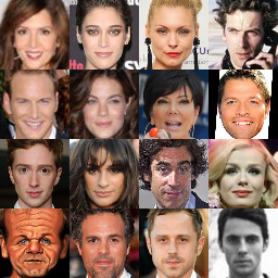
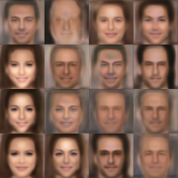
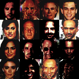
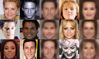
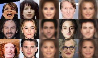
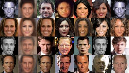
We used Adam optimizer with batch size 1. Note that it makes no sense using a value of batch size other than 1. The reason being, in our proposed framework, each pair of voice and face is unique, thus it requires a unique set of network weights to perform generation. After grid search, we finalized the learning rate to be 0.0002, = 0.5, and = 0.999. Also, we trained the discriminator and generator with ratio 1:1, using = 1, = 10, = 1, = 1, . Results for this part are illustrated in Figure 3.
To validate the the model indeed performs as we expect, we present visualizations of the following settings:
-
•
Fix the proposal face, change the input voice. This is to confirm our model’s ability of generating different faces based on the same proposal face.
-
•
Fix the input voice, change the proposal face. This is to confirm our model’s ability of generating the target face based on different proposal faces.
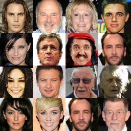
Example results are shown in Figures 3 and 3 respectively. Results are random selections from our data and are not cherry picked. We can confirm that our model is able to generate a target face by performing necessary modifications to the proposal faces. Figures 3, 3, 3, 3 also compare faces generated from voices by our CAE to those generated by the technique from [10], which is currently a state of the art. For example, the faces in the upper left corner of (a), (b), (c), (d) represent the original input face, corresponding face of the target voice, generated face using our model, generated face using [10] respectively.
4.3 Evaluation
Evaluation of generative models like GANs models is always tricky and several methods have been proposed [18] for it. Considering the speciality of our task which requires the output image to keep features from both faces, however, classification error [10], Fréchet Inception Distance (FID) [19] and reconstruction error, which are the most common evaluation metrics, are not good options. Instead, we resort to human subjective votes – one of the most mature and solid method – as our first evaluation metric, and retrieval as our second.
4.3.1 Human subjective evaluation
The human subject method is broadly adopted in many generative models [20, 21, 22, 23] because of its intuitiveness and reliability when the number of samples becomes large. In this task, we conducted human subjective evaluation through interviews. To ensure the feasibility and reliability, the interviewers were first asked to finish a real-image mapping, which contains two images and their corresponding voices, and map the images with the voices. A 89% mapping accuracy was obtained from 20 subjects, performing 100 tests each, validating our conjecture: human subjective mapping between voices and images is reliable and robust. Next, they were shown a generated face image that was synthesized with our model, its corresponding voice audio, and another randomly generated face image which has the same gender, then asked to map the voice to one of the two images.
All the interviewers were asked to rate in total 100 rounds of tests. Finally, a 72% mapping accuracy was achieved. Based on the result, we are convinced we have reached our goal – to generate a face behind a voice by only modifying necessary features from a proposal face.
| Task | Accuracy (%) |
|---|---|
| real image maping | 89 |
| generated image mapping(CAE) | 72 |
| random | 50 |
4.3.2 Feature similarity and face retrieval
To make our results more convincing, we adopted the evaluation strategies from [3]. We reused the face embedding network we got from our training to get three 64-dimensional feature vectors for the generated face images, original input image and the corresponding image of the voice respectively. Then we calculated the cosine similarity between the generated image’s embedding vector and the other two. The result is shown in table 3, indicating out results complete the goal of maintaining features from both faces.
| Mapping pair | cos |
|---|---|
| 0.32 | |
| 0.42 | |
| random mapping | 0.21 |
In addition to this, we also utilized face retrieval, where we reused the classifier we obtained from training again and injected the generated face image as input, and got top 5 faces retrieved, i.e. whose corresponding value in the output vector of classifier lies in top 5. If the original face was in the top 5, we marked it as a successful retrieval. The successful ratios of our model was 21%, in a 500 images retrieval task. Some samples are shown in Figure 4.
5 Conclusion
We presented a novel model, the Controlled AutoEncoder, for modifying human face images to match input voices. The model uses conditioning voice input as a controller, to modify output images. While this is seen to work well in the setting of conditional production of face images, we believe the model has wider applicability in other problems, which we are investigating. Within the proposed framework too, much room remains for improvement. Current results seem to indicate that the entire face is modified, as opposed to specific components of it. We are conducting investigations into whether finer control may be exercised over this process.
References
- [1] L. L. Zhu and M. Beauchamp, “Mouth and voice: A relationship between visual and auditory preference in the human superior temporal sulcus,” The Journal of neuroscience : the official journal of the Society for Neuroscience, vol. 37, 02 2017.
- [2] C. Kim, H. V. Shin, T.-H. Oh, A. Kaspar, M. Elgharib, and W. Matusik, “On learning associations of faces and voices,” in Proceedings of Asian Conference on Computer Vision (ACCV), 2018.
- [3] T.-H. Oh, T. Dekel, C. Kim, I. Mosseri, W. T. Freeman, M. Rubinstein, and W. Matusik, “Speech2face: Learning the face behind a voice,” in Proceedings of the IEEE/CVF Conference on Computer Vision and Pattern Recognition (CVPR), June 2019.
- [4] N. Sadoughi and C. Busso, “Speech-driven expressive talking lips with conditional sequential generative adversarial networks,” CoRR, vol. abs/1806.00154, 2018.
- [5] O. Wiles, A. Koepke, and A. Zisserman, “X2face: A network for controlling face generation by using images, audio, and pose codes,” in European Conference on Computer Vision, 2018.
- [6] Y. Wen, M. A. Ismail, W. Liu, B. Raj, and R. Singh, “Disjoint mapping network for cross-modal matching of voices and faces,” in International Conference on Learning Representations, 2019.
- [7] A. Nagrani, S. Albanie, and A. Zisserman, “Seeing voices and hearing faces: Cross-modal biometric matching,” in IEEE Conference on Computer Vision and Pattern Recognition, 2018.
- [8] A. Duarte, F. Roldan, M. Tubau, J. Escur, S. Pascual, A. Salvador, E. Mohedano, K. McGuinness, J. Torres, and X. G. i Nieto, “Wav2pix: Speech-conditioned face generation using generative adversarial networks,” in 2019 IEEE International Conference on Acoustics, Speech and Signal Processing (ICASSP). IEEE, 2019.
- [9] H. Li, B. Li, S. Tan, and J. Huang, “Detection of Deep Network Generated Images Using Disparities in Color Components,” arXiv e-prints, p. arXiv:1808.07276, Aug. 2018.
- [10] Y. Wen, B. Raj, and R. Singh, “Face reconstruction from voice using generative adversarial networks,” in Advances in Neural Information Processing Systems, 2019, pp. 5266–5275.
- [11] Y. Bian, J. Wang, J. J. Jun, and X.-Q. Xie, “Deep convolutional generative adversarial network (dcgan) models for screening and design of small molecules targeting cannabinoid receptors,” Molecular pharmaceutics, vol. 16, no. 11, p. 4451—4460, November 2019.
- [12] H. Chen and C. Lu, “Nested variance estimating vae/gan for face generation,” in 2019 International Joint Conference on Neural Networks (IJCNN), 2019, pp. 1–8.
- [13] O. Ronneberger, P. Fischer, and T. Brox, “U-net: Convolutional networks for biomedical image segmentation,” LNCS, vol. 9351, pp. 234–241, 2015.
- [14] Y. Choi, M. Choi, M. Kim, J.-W. Ha, S. Kim, and J. Choo, “Stargan: Unified generative adversarial networks for multi-domain image-to-image translation,” in Proceedings of the IEEE Conference on Computer Vision and Pattern Recognition, 2018.
- [15] J. Zhu, T. Park, P. Isola, and A. A. Efros, “Unpaired image-to-image translation using cycle-consistent adversarial networks,” in 2017 IEEE International Conference on Computer Vision (ICCV), 2017, pp. 2242–2251.
- [16] A. Nagrani, J. S. Chung, and A. Zisserman, “Voxceleb: a large-scale speaker identification dataset,” in INTERSPEECH, 2017.
- [17] O. M. Parkhi, A. Vedaldi, A. Zisserman et al., “Deep face recognition.” in bmvc, vol. 1, no. 3, 2015, p. 6.
- [18] A. Borji, “Pros and cons of gan evaluation measures,” Computer Vision and Image Understanding, vol. 179, pp. 41 – 65, 2019.
- [19] M. Heusel, H. Ramsauer, T. Unterthiner, B. Nessler, and S. Hochreiter, “Gans trained by a two time-scale update rule converge to a local nash equilibrium,” in Advances in Neural Information Processing Systems 30, 2017, pp. 6626–6637.
- [20] S. Zhou, M. L. Gordon, R. Krishna, A. Narcomey, F. Li, and M. Bernstein, “HYPE: A benchmark for human eye perceptual evaluation of generative models,” in Advances in Neural Information Processing Systems 32: Annual Conference on Neural Information Processing Systems 2019, NeurIPS 2019, 8-14 December 2019, Vancouver, BC, Canada, 2019, pp. 3444–3456.
- [21] D. Bau, J.-Y. Zhu, H. Strobelt, B. Zhou, J. B. Tenenbaum, W. T. Freeman, and A. Torralba, “Gan dissection: Visualizing and understanding generative adversarial networks,” in Proceedings of the International Conference on Learning Representations (ICLR), 2019.
- [22] K. Lin, D. Li, X. He, Z. Zhang, and M.-T. Sun, “Adversarial ranking for language generation,” ser. NIPS’17, 2017, p. 3158–3168.
- [23] L. Yu, W. Zhang, J. Wang, and Y. Yu, “Seqgan: Sequence generative adversarial nets with policy gradient,” in Proceedings of the Thirty-First AAAI Conference on Artificial Intelligence, ser. AAAI’17. AAAI Press, 2017, p. 2852–2858.