Scalar conservation laws with stochastic discontinuous flux function

Lukas Brencher†, Corresponding author. (lukas.brencher@mathematik.uni-stuttgart.de)    Andrea Barth University of Stuttgart, Allmandring 5b, 70569 Stuttgart, Germany
Abstract

A variety of real-world applications are modeled via hyperbolic conservation laws. To account for uncertainties or insufficient measurements, random coefficients may be incorporated. These random fields may depend discontinuously on the state space, e.g., to represent permeability in a heterogeneous or fractured medium. We introduce a suitable admissibility criterion for the resulting stochastic discontinuous-flux conservation law and prove its well-posedness. Therefore, we ensure the pathwise existence and uniqueness of the corresponding deterministic setting and present a novel proof for the measurability of the solution, since classical approaches fail in the discontinuous-flux case. As an example of the developed theory, we present a specific advection coefficient, which is modeled as a sum of a continuous random field and a pure jump field. This random field is employed in the stochastic conservation law, in particular a stochastic Burgers’ equation, for numerical experiments. We approximate the solution to this problem via the Finite Volume method and introduce a new meshing strategy that accounts for the resulting standing wave profiles caused by the flux-discontinuities. The ability of this new meshing method to reduce the sample-wise variance is demonstrated in numerous numerical investigations.

keywords:
Stochastic conservation laws, discontinuous flux function, stochastic entropy solution, Finite Volume method, non-continuous random fields, fractured media, jump-advection coefficient
AMS:
65M55, 60G60, 60H15, 35R60, 60H35, 65C30, 46N20, 35B30, 35F20, 35F25, 35L02, 35L03, 35L65

1 Introduction

Conservation laws are widely used to model problems in various applications, such as fluid and gas dynamics [4, 29], hydrodynamics [19], nonlinear elasticity, semiconductor simulation and many more. We refer to the books of Dafermos [21] and LeVeque [35] and the references therein for more applications. There are two natural extensions of models based on conservation laws:

  1. (i)

    One may want to allow the flux function to depend (possibly discontinuously) on the state space, e.g., to model heterogeneities or fractures in a porous medium for subsurface or two-phase flow simulations [4, 29, 26]. This approach is also used for many other models in a variety of fields, e.g., vehicular traffic flows [5, 20], statistical mechanics [19], sedimentation [18] and kidney physiology [42].

  2. (ii)

    One might be interested in including stochastic terms, e.g., a stochastic flux function [28, 36, 37] or a stochastic source [30, 32], to account for uncertainties or insufficient data in the underlying model.

To combine both extensions, we consider a stochastic conservation law, where the flux function depends discontinuously on the state space. In this paper, we are concerned with well-posedness of the solution to such a stochastic conservation law. A special case of the considered stochastic conservation law are flux functions, in which a discontinuous random coefficient is incorporated. This random coefficient is constructed via a continuous part and a discontinuous part, which is inspired by the unique characterization of Lévy processes via the Lévy-Khintchine formula [7, 31]. By this formula, every Lévy process can be seen as the composition of three independent components, namely, a drift term, a Brownian motion and a pure jump process.

The paper is structured as follows: In the remainder of this section, we discuss existing results on conservation laws with discontinuous flux function in Section 1.1, before stating existing results on stochastic conservation laws in Section 1.2. In the following section, we state the considered problem and show our main result: the well-posedness of pathwise solutions. In Section 3, we define a random coefficient and its numerical approximation. Afterwards, we introduce a numerical discretization of the stochastic conservation law with discontinuous random coefficient and investigate the convergence of the approximations in numerical experiments.

1.1 Conservation laws with spatial discontinuities

We are interested in scalar conservation laws with a flux that depends discontinuously on the spatial variable. For t𝕋𝑡𝕋t\in\mathbb{T}, where 𝕋𝕋\mathbb{T}\subset\mathbb{R} denotes the time interval, the conservation law is given by

(1) ut+𝔣(x,u)xsubscript𝑢𝑡𝔣subscript𝑥𝑢𝑥\displaystyle u_{t}+\mathfrak{f}(x,u)_{x} =0absent0\displaystyle=0 in ×𝕋,in 𝕋\displaystyle\text{in }\mathbb{R}\times\mathbb{T}\ ,
u(x,0)𝑢𝑥0\displaystyle u(x,0) =u0(x)absentsubscript𝑢0𝑥\displaystyle=u_{0}(x) in ,in \displaystyle\text{in }\mathbb{R}\ ,

where u0(x)L()subscript𝑢0𝑥superscript𝐿u_{0}(x)\in L^{\infty}(\mathbb{R}) denotes the initial condition of the partial differential equation. Furthermore, the flux 𝔣𝔣\mathfrak{f} is assumed to depend discontinuously on space. In case the flux function 𝔣𝔣\mathfrak{f} is sufficiently smooth, well-posedness of (1) is well established [15, 34]. However, even with smooth initial data and a sufficiently smooth flux function, the solution might develop discontinuities. Therefore, weak solutions are sought, but they are not unique without an additional admissibility criterion selecting the physical solution. In case of a smooth space dependency of the flux 𝔣𝔣\mathfrak{f} the entropy condition was described by Kružkov [34]. A function uL(×𝕋;)𝑢superscript𝐿𝕋u\in L^{\infty}(\mathbb{R}\times\mathbb{T};\mathbb{R}) is an entropy solution of (1) if for all m𝑚m\in\mathbb{R} it satisfies the following inequality in the distributional sense:

(2) t\MT@delim@Auto\abs@starum+x(sign(um)(𝔣(x,u)𝔣(x,m)))+sign(um)x𝔣(x,m)0.𝑡\MT@delim@Auto\abs@star𝑢𝑚𝑥sign𝑢𝑚𝔣𝑥𝑢𝔣𝑥𝑚sign𝑢𝑚𝑥𝔣𝑥𝑚0\frac{\partial}{\partial t}\MT@delim@Auto\abs@star{u-m}+\frac{\partial}{\partial x}\left(\operatorname{sign}(u-m)(\mathfrak{f}(x,u)-\mathfrak{f}(x,m))\right)+\operatorname{sign}(u-m)\frac{\partial}{\partial x}\mathfrak{f}(x,m)\leq 0\ .

For discontinuous flux functions, the Kružkov entropy condition (2) does not make sense due to the term sign(um)x𝔣(x,m)sign𝑢𝑚𝑥𝔣𝑥𝑚\operatorname{sign}(u-m)\frac{\partial}{\partial x}\mathfrak{f}(x,m). To overcome this difficulty, a variety of criteria were introduced to select the appropriate weak solution. However, for some problems, different selection criteria might lead to different solutions. Therefore, the solution we are seeking might depend on the context.

A common approach to define a selection criterion is to require the usual entropy condition, when the flux is continuous, and impose additional constraints at the discontinuities (see, e.g., [2, 16, 25]). A natural choice of such a condition is the continuity of the flux at the heterogeneities, given by the Rankine-Hugoniot condition

(3) 𝔣(x,u(x,t))=𝔣(x+,u(x+,t))t𝕋.formulae-sequence𝔣superscript𝑥𝑢superscript𝑥𝑡𝔣superscript𝑥𝑢superscript𝑥𝑡𝑡𝕋\mathfrak{f}(x^{-},u(x^{-},t))=\mathfrak{f}(x^{+},u(x^{+},t))\quad t\in\mathbb{T}.

However, this condition is not sufficient to select an unique solution. Note that for discontinuous flux functions this procedure requires the existence of traces along the discontinuities, which implies the spatial points to occur at isolated points. For an exhaustive review of different selection criteria, the reader is referred to [6], where each existing admissibility criterion is associated to a so-called Germ.

1.1.1 Audusse-Perthame adapted entropy formulation

The theory of adapted-entropy solutions for conservation laws was introduced by Audusse and Perthame [8] in 2005, based on the ideas of Baiti and Jenssen [9] from 1997. The provided framework is formulated, such that no additional interface conditions are imposed. As a result, the existence of traces is not required, since the discontinuity points are not distinguished separately. This makes it possible to include an infinite number of discontinuity points in the flux function.

The main idea of the framework is to adapt the classical Kružkhov entropy condition (2) in such a way that the troublesome term vanishes. Therefore, instead of the classical Kružkhov [34] entropies (\MT@delim@Auto\abs@starum)msubscript\MT@delim@Auto\abs@star𝑢𝑚𝑚(\MT@delim@Auto\abs@star{u-m})_{m\in\mathbb{R}}, adapted entropies (\MT@delim@Auto\abs@starumα(x))αsubscript\MT@delim@Auto\abs@star𝑢subscript𝑚𝛼𝑥𝛼(\MT@delim@Auto\abs@star{u-m_{\alpha}(x)})_{\alpha\in\mathbb{R}} are considered. Here, mα(x)subscript𝑚𝛼𝑥m_{\alpha}(x) denotes the unique solution of the problem

(4) 𝔣(x,mα(x))=αfor a.e. x.formulae-sequence𝔣𝑥subscript𝑚𝛼𝑥𝛼for a.e. 𝑥\mathfrak{f}(x,m_{\alpha}(x))=\alpha\quad\text{for a.e. }x\in\mathbb{R}\ .

The existence and uniqueness of mα(x)subscript𝑚𝛼𝑥m_{\alpha}(x) in (4) is guaranteed by the following assumptions:

Assumption 1 (Assumption on the flux function: adapted entropy formulation).
  1. (A-1)

    The flux function 𝔣(x,ρ)𝔣𝑥𝜌\mathfrak{f}(x,\rho) is continuous at all points of (𝒩)×𝒩(\mathbb{R}\setminus\mathcal{N})\times\mathbb{R}, where 𝒩𝒩\mathcal{N}\subset\mathbb{R} is a closed set of measure zero that contains the discontinuity points of 𝔣(,ρ)𝔣𝜌\mathfrak{f}(\cdot,\rho).

  2. (A-2)

    There exist two functions g,g+C0()subscript𝑔subscript𝑔superscript𝐶0g_{-},g_{+}\in C^{0}(\mathbb{R}) such that for all x𝑥x\in\mathbb{R} it holds that g(ρ)|𝔣(x,ρ)|g+(ρ)subscript𝑔𝜌𝔣𝑥𝜌subscript𝑔𝜌g_{-}(\rho)\leq|\mathfrak{f}(x,\rho)|\leq g_{+}(\rho), where gsubscript𝑔g_{-} is a non-negative (non-strictly) decreasing then increasing function which satisfies |g(±)|=+subscript𝑔plus-or-minus|g_{-}(\pm\infty)|=+\infty.

  3. (A-3)

    There exists a function uM(x)::subscript𝑢𝑀𝑥u_{M}(x):\mathbb{R}\rightarrow\mathbb{R} and a constant M0subscript𝑀0M_{0} such that for x𝒩𝑥𝒩x\in\mathbb{R}\setminus\mathcal{N}, 𝔣(x,)𝔣𝑥\mathfrak{f}(x,\cdot) is a locally Lipschitz one-to-one function from (,uM(x)]subscript𝑢𝑀𝑥(-\infty,u_{M}(x)] and [uM(x),+)subscript𝑢𝑀𝑥[u_{M}(x),+\infty) to [M0,+)subscript𝑀0[M_{0},+\infty) (or (,M0]subscript𝑀0(-\infty,M_{0}]) that satisfies 𝔣(x,uM(x))=0𝔣𝑥subscript𝑢𝑀𝑥0\mathfrak{f}(x,u_{M}(x))=0 and with common Lipschitz constant LIsubscript𝐿𝐼L_{I} for all x𝒩𝑥𝒩x\in\mathbb{R}\setminus\mathcal{N} and all uI𝑢𝐼u\in I, where I𝐼I\subset\mathbb{R} is any bounded interval.

Alternatively, instead of (A-3) we may consider the assumption

  1. (A-3’)

    For x𝒩𝑥𝒩x\in\mathbb{R}\setminus\mathcal{N}, the flux function 𝔣(x,)𝔣𝑥\mathfrak{f}(x,\cdot) is a locally Lipschitz one-to-one function from \mathbb{R} to \mathbb{R} with common Lipschitz constant LIsubscript𝐿𝐼L_{I} for all x𝒩𝑥𝒩x\in\mathbb{R}\setminus\mathcal{N} and all uI𝑢𝐼u\in I, where I𝐼I\subset\mathbb{R} is any bounded interval.

In case the flux function satisfies Assumptions (A-1)-(A-3), for any constant α[M0,)𝛼subscript𝑀0\alpha\in[M_{0},\infty) (or α(,M0]𝛼subscript𝑀0\alpha\in(-\infty,M_{0}]), there exist two steady-state solutions mα+(x)subscriptsuperscript𝑚𝛼𝑥m^{+}_{\alpha}(x) from \mathbb{R} to [uM(x),)subscript𝑢𝑀𝑥[u_{M}(x),\infty) and mα(x)subscriptsuperscript𝑚𝛼𝑥m^{-}_{\alpha}(x) from \mathbb{R} to (,uM(x)]subscript𝑢𝑀𝑥(-\infty,u_{M}(x)] of (1) satisfying (4). In case of Assumptions (A-1)-(A-3’), the two steady state solutions coincide, which is even simpler.

Now, the adapted entropies (\MT@delim@Auto\abs@starumα(x))αsubscript\MT@delim@Auto\abs@star𝑢subscript𝑚𝛼𝑥𝛼(\MT@delim@Auto\abs@star{u-m_{\alpha}(x)})_{\alpha\in\mathbb{R}} allow us to define adapted entropy solutions.

Definition 2 (adapted entropy solution).

A function uL(×𝕋)C0(𝕋,Lloc1())𝑢superscript𝐿𝕋superscript𝐶0𝕋subscriptsuperscript𝐿1locu\in L^{\infty}(\mathbb{R}\times\mathbb{T})\cap C^{0}(\mathbb{T},L^{1}_{\text{loc}}(\mathbb{R})) is an adapted entropy solution of (1) on ×𝕋𝕋\mathbb{R}\times\mathbb{T}, provided that for each α[M0,)𝛼subscript𝑀0\alpha\in[M_{0},\infty) (or α(,M0]𝛼subscript𝑀0\alpha\in(-\infty,M_{0}]) and the corresponding two steady-state solutions mα±(x)subscriptsuperscript𝑚plus-or-minus𝛼𝑥m^{\pm}_{\alpha}(x) of (1), the following inequality holds in the sense of distributions:

(5) t\MT@delim@Auto\abs@staru(x,t)mα±(x)+x(sign(u(x,t)mα±(x))(𝔣(x,u(x,t))𝔣(x,mα±(x))))0.𝑡\MT@delim@Auto\abs@star𝑢𝑥𝑡subscriptsuperscript𝑚plus-or-minus𝛼𝑥𝑥sign𝑢𝑥𝑡subscriptsuperscript𝑚plus-or-minus𝛼𝑥𝔣𝑥𝑢𝑥𝑡𝔣𝑥subscriptsuperscript𝑚plus-or-minus𝛼𝑥0\frac{\partial}{\partial t}\MT@delim@Auto\abs@star{u(x,t)-m^{\pm}_{\alpha}(x)}+\frac{\partial}{\partial x}\left(\operatorname{sign}\left(u(x,t)-m^{\pm}_{\alpha}(x)\right)(\mathfrak{f}(x,u(x,t))-\mathfrak{f}(x,m^{\pm}_{\alpha}(x)))\right)\leq 0\ .

This formulation guarantees the uniqueness of solutions, since the doubling of variables approach can be applied. The existence was shown in [19] via the reduction of measure-valued solutions. However, to the best of the author’s knowledge, extending the adapted entropy formulation to multidimensional conservation laws is still an open problem.

1.2 Stochastic conservation laws

The field of stochastic conservation laws has attracted considerable attention in the past 20 years. The concept of stochastic weak and entropy solutions was initially introduced by Holden and Risebro in [28], who considered nonlinear hyperbolic problems with time-dependent stochastic source terms. This concept was further developed by Kim in [32] and extended to conservation laws with multiplicative noise, see [22] for Gaussian and [14] for Lévy noise. In [13], Bauzet et al. used the concept of Kružkov’s entropy formulation and measure-valued solutions to establish existence and uniqueness of entropy solutions for multi-dimensional nonlinear conservation laws with multiplicative stochastic perturbation. Recently, Karlsen and Storrøsten generalized this approach by allowing the stochastic Kružkov entropy condition to contain Malliavin differentiable random variables [30]. They also provided existence and uniqueness results for this extended framework.

In 2013 Lions [36] considered scalar conservation laws with rough stochastic fluxes and extended this in [37] to the case, where the rough stochastic flux function is space dependent. The field of scalar conservation laws with rough fluxes combined with stochastic forcing was also considered by Hofmanová in [27], who proved well-posedness for the corresponding kinetic formulation and its solution.

Stochastic systems of conservation laws were considered by Mishra and Schwab in [38], who introduced the uncertainty via random initial data. In [43] Poëtte et al. considered hyperbolic systems with a randomly perturbed flux function and showed the hyperbolicity of a stochastic Galerkin representation. The stochastic Galerkin representation was later extended by [48] and [17]. A comprehensive discussion on current numerical methods for hyperbolic systems of conservation laws can be found in [1].

In [41], Mishra et al. considered the numerical approximation of scalar conservation laws in several space dimensions with random flux functions and also showed convergence analysis for the multilevel Monte Carlo finite volume method [38, 40, 39]. Another numerical approximation was introduced by Risebro et. al. [44], who proposed a multilevel Monte Carlo front tracking algorithm for stochastic scalar conservation laws with bounded random flux function. This approach was generalized in [33] to the case of random degenerate convection-diffusion equations.

Recently, Barth and Stein [10] considered semilinear hyperbolic stochastic partial differential equations, which are driven by Lévy noise and provided a fully discrete numerical approximation for this problem.

2 Stochastic scalar conservation laws with discontinuous flux functions

Let (Ω,𝒜,)Ω𝒜(\Omega,\mathcal{A},\mathbb{P}) be a complete probability space and let 𝕋:=[0,T]0assign𝕋0𝑇subscriptabsent0\mathbb{T}:=[0,T]\subset\mathbb{R}_{\geq 0} be a time interval for some T>0𝑇subscriptabsent0T\in\mathbb{R}_{>0}. We consider a scalar, one-dimensional conservation law of the form

(6) ut+𝔣(ω,x,u)xsubscript𝑢𝑡𝔣subscript𝜔𝑥𝑢𝑥\displaystyle u_{t}+\mathfrak{f}(\omega,x,u)_{x} =0absent0\displaystyle=0 in Ω××𝕋,in Ω𝕋\displaystyle\text{in }\Omega\times\mathbb{R}\times\mathbb{T}\ ,
u(ω,x,0)𝑢𝜔𝑥0\displaystyle u(\omega,x,0) =u0(ω,x)absentsubscript𝑢0𝜔𝑥\displaystyle=u_{0}(\omega,x) in Ω×,in Ω\displaystyle\text{in }\Omega\times\mathbb{R}\ ,

where u0Lp(Ω,L())subscript𝑢0superscript𝐿𝑝Ωsuperscript𝐿u_{0}\in L^{p}(\Omega,L^{\infty}(\mathbb{R})) denotes the stochastic initial condition of the partial differential equation. We impose the following assumptions on the stochastic flux function:

Assumption 3 (Pathwise assumption on the stochastic flux function).

We assume the stochastic discontinuous flux function to satisfy the following assumptions for every ωΩ𝜔Ω\omega\in\Omega:

  1. (B-1)

    The flux function 𝔣(ω,,)𝔣𝜔\mathfrak{f}(\omega,\cdot,\cdot) is continuous at all points of (𝒩(ω))×𝒩𝜔(\mathbb{R}\setminus\mathcal{N}(\omega))\times\mathbb{R} with 𝒩(ω)𝒩𝜔\mathcal{N}(\omega)\subset\mathbb{R} a closed set of measure zero that contains the discontinuity points of 𝔣(ω,,ρ)𝔣𝜔𝜌\mathfrak{f}(\omega,\cdot,\rho).

  2. (B-2)

    There exist two functions g(ω,),g+(ω,)C0()subscript𝑔𝜔subscript𝑔𝜔superscript𝐶0g_{-}(\omega,\cdot),g_{+}(\omega,\cdot)\in C^{0}(\mathbb{R}) such that for all x𝑥x\in\mathbb{R} it holds that g(ω,ρ)|𝔣(ω,x,ρ)|g+(ω,ρ)subscript𝑔𝜔𝜌𝔣𝜔𝑥𝜌subscript𝑔𝜔𝜌g_{-}(\omega,\rho)\leq|\mathfrak{f}(\omega,x,\rho)|\leq g_{+}(\omega,\rho), where g(ω,)subscript𝑔𝜔g_{-}(\omega,\cdot) is a decreasing then increasing function with g(ω,ρ)0subscript𝑔𝜔𝜌0g_{-}(\omega,\rho)\geq 0 and |g(ω,±)|=+subscript𝑔𝜔plus-or-minus|g_{-}(\omega,\pm\infty)|=+\infty.

  3. (B-3)

    There exists a function uM(ω,x):Ω×:subscript𝑢𝑀𝜔𝑥Ωu_{M}(\omega,x):\Omega\times\mathbb{R}\rightarrow\mathbb{R} and a constant M0subscript𝑀0M_{0}\in\mathbb{R} such that for x𝒩(ω)𝑥𝒩𝜔x\in\mathbb{R}\setminus\mathcal{N}(\omega), the flux function 𝔣(ω,x,)𝔣𝜔𝑥\mathfrak{f}(\omega,x,\cdot) is locally Lipschitz and one-to-one from (,uM(ω,x)]subscript𝑢𝑀𝜔𝑥(-\infty,u_{M}(\omega,x)] and [uM(ω,x),+)subscript𝑢𝑀𝜔𝑥[u_{M}(\omega,x),+\infty) to [M0,+)subscript𝑀0[M_{0},+\infty) (or (,M0]subscript𝑀0(-\infty,M_{0}]). Further it satisfies 𝔣(ω,x,uM(ω,x))=M0𝔣𝜔𝑥subscript𝑢𝑀𝜔𝑥subscript𝑀0\mathfrak{f}(\omega,x,u_{M}(\omega,x))=M_{0} with common Lipschitz constant LIsubscript𝐿𝐼L_{I} for all x𝒩(ω)𝑥𝒩𝜔x\in\mathbb{R}\setminus\mathcal{N}(\omega) and all uI𝑢𝐼u\in I, where I𝐼I\subset\mathbb{R} is any bounded interval.

Alternatively, instead of (B-3) we may consider the assumption

  1. (B-3’)

    For x𝒩(ω)𝑥𝒩𝜔x\in\mathbb{R}\setminus\mathcal{N}(\omega), the flux function 𝔣(ω,x,)𝔣𝜔𝑥\mathfrak{f}(\omega,x,\cdot) is locally Lipschitz and one-to-one from \mathbb{R} to \mathbb{R} with common Lipschitz constant LIsubscript𝐿𝐼L_{I} for all x𝒩(ω)𝑥𝒩𝜔x\in\mathbb{R}\setminus\mathcal{N}(\omega) and all uI𝑢𝐼u\in I, where I𝐼I\subset\mathbb{R} is any bounded interval.

Example 4 (Multiplicative flux).

One example of stochastic flux functions satisfying Assumption 3 is

(7) 𝔣(ω,x,ρ)=a(ω,x)f(ρ).𝔣𝜔𝑥𝜌𝑎𝜔𝑥𝑓𝜌\mathfrak{f}(\omega,x,\rho)=a(\omega,x)f(\rho).

Here, a(ω,x)𝑎𝜔𝑥a(\omega,x) is continuous in x𝑥x\in\mathbb{R} except on a closed set 𝒩𝒩\mathcal{N} of measure zero that might depend on ωΩ𝜔Ω\omega\in\Omega (assuring Assumption (B-1)). Further, the coefficient a(ω,x)𝑎𝜔𝑥a(\omega,x) has positive spatially bounded paths, i.e., 0<a(ω)a(ω,x)a+(ω)<0subscript𝑎𝜔𝑎𝜔𝑥subscript𝑎𝜔0<a_{-}(\omega)\leq a(\omega,x)\leq a_{+}(\omega)<\infty for some constants asubscript𝑎a_{-} and a+subscript𝑎a_{+} that might depend on ωΩ𝜔Ω\omega\in\Omega (assuring Assumption (B-2)). The flux function f(ρ)𝑓𝜌f(\rho) is locally Lipschitz continuous and is either monotone (Assumption (B-3’)) or convex (or concave) with f(uM(ω,x))=0𝑓subscript𝑢𝑀𝜔𝑥0f(u_{M}(\omega,x))=0 for some uMsubscript𝑢𝑀u_{M}, in which case we have M0=0subscript𝑀00M_{0}=0 (Assumption (B-3)).

Remark 5 (Existence of stochastic steady state solutions).

To define a meaningful entropy solution, we have to ensure the well-posedness of the stochastic steady state equation

(8) 𝔣(ω,x,mα±(ω,x))=αfor a.e. x.formulae-sequence𝔣𝜔𝑥subscriptsuperscript𝑚plus-or-minus𝛼𝜔𝑥𝛼for a.e. 𝑥\mathfrak{f}(\omega,x,m^{\pm}_{\alpha}(\omega,x))=\alpha\quad\text{for a.e. }x\in\mathbb{R}\ .

If assumptions (B-1)-(B-3) are satisfied, then for any constant α[M0,)𝛼subscript𝑀0\alpha\in[M_{0},\infty) (or α(,M0]𝛼subscript𝑀0\alpha\in(-\infty,M_{0}]) and any ωΩ𝜔Ω\omega\in\Omega, there exist two steady state solutions mα+:Ω×[M0,):subscriptsuperscript𝑚𝛼Ωsubscript𝑀0m^{+}_{\alpha}:\Omega\times\mathbb{R}\rightarrow[M_{0},\infty) and mα:Ω×(,M0]:subscriptsuperscript𝑚𝛼Ωsubscript𝑀0m^{-}_{\alpha}:\Omega\times\mathbb{R}\rightarrow(-\infty,M_{0}] of (6) satisfying (8). For the case (B-1)-(B-3’) the two steady state solutions coincide, i.e., mα+(ω,x)=mα(ω,x)subscriptsuperscript𝑚𝛼𝜔𝑥subscriptsuperscript𝑚𝛼𝜔𝑥m^{+}_{\alpha}(\omega,x)=m^{-}_{\alpha}(\omega,x).

The steady state solutions defined in Remark 5 allow us to introduce the partially adapted Kružkhov entropies Eα(ω,x,u)=|umα±(ω,x)|subscript𝐸𝛼𝜔𝑥𝑢𝑢subscriptsuperscript𝑚plus-or-minus𝛼𝜔𝑥E_{\alpha}(\omega,x,u)=|u-m^{\pm}_{\alpha}(\omega,x)|, which lead to the notion of pathwise adapted entropy solutions.

Definition 6 (Pathwise adapted entropy solution).

Let ωΩ𝜔Ω\omega\in\Omega be fixed. A function u(ω,,)L(𝕋×)C0(𝕋,Lloc1())𝑢𝜔superscript𝐿𝕋superscript𝐶0𝕋subscriptsuperscript𝐿1locu(\omega,\cdot,\cdot)\in L^{\infty}(\mathbb{T}\times\mathbb{R})\cap C^{0}(\mathbb{T},L^{1}_{\text{loc}}(\mathbb{R})) is an adapted entropy solution of (6) on ×𝕋𝕋\mathbb{R}\times\mathbb{T}, provided that for each α[M0,)𝛼subscript𝑀0\alpha\in[M_{0},\infty) (or α(,M0]𝛼subscript𝑀0\alpha\in(-\infty,M_{0}]) and the corresponding two steady-state solutions mα±(ω,x)subscriptsuperscript𝑚plus-or-minus𝛼𝜔𝑥m^{\pm}_{\alpha}(\omega,x) of (8), the inequality

(9) |u(ω,x,t)mα±(ω,x)|tϕ(x,t)dtdx𝑢𝜔𝑥𝑡subscriptsuperscript𝑚plus-or-minus𝛼𝜔𝑥𝑡italic-ϕ𝑥𝑡d𝑡d𝑥\displaystyle\int\Big{|}u(\omega,x,t)-m^{\pm}_{\alpha}(\omega,x)\Big{|}\frac{\partial}{\partial t}\phi(x,t)\operatorname{d}\!{t}\operatorname{d}\!{x}
+sign(u(ω,x,t)mα±(ω,x))(𝔣(ω,x,u(ω,x,t))α)xϕ(x,t)dtdxsign𝑢𝜔𝑥𝑡subscriptsuperscript𝑚plus-or-minus𝛼𝜔𝑥𝔣𝜔𝑥𝑢𝜔𝑥𝑡𝛼𝑥italic-ϕ𝑥𝑡d𝑡d𝑥\displaystyle\hskip 42.67912pt+\int\operatorname{sign}\Big{(}u(\omega,x,t)-m^{\pm}_{\alpha}(\omega,x)\Big{)}\Big{(}\mathfrak{f}(\omega,x,u(\omega,x,t))-\alpha\Big{)}\frac{\partial}{\partial x}\phi(x,t)\operatorname{d}\!{t}\operatorname{d}\!{x}
+|u0(ω,x)mα±(ω,x)|ϕ(x,0)dx0subscript𝑢0𝜔𝑥subscriptsuperscript𝑚plus-or-minus𝛼𝜔𝑥italic-ϕ𝑥0d𝑥0\displaystyle\hskip 85.35826pt+\int\Big{|}u_{0}(\omega,x)-m^{\pm}_{\alpha}(\omega,x)\Big{|}\phi(x,0)\operatorname{d}\!{x}\geq 0

holds for every test function ϕCc(×𝕋;0)italic-ϕsubscriptsuperscript𝐶𝑐𝕋subscriptabsent0\phi\in C^{\infty}_{c}(\mathbb{R}\times\mathbb{T};\mathbb{R}_{\geq 0}).

As a direct consequence of Assumption 3 and the definition of pathwise adapted entropy solutions, we can conclude the following lemma.

Lemma 7.

Let Assumption (B-2) be satisfied and fix an arbitrary ωΩ𝜔Ω\omega\in\Omega. Furthermore, suppose u(ω,,)L(𝕋×)C0(𝕋,Lloc1())𝑢𝜔superscript𝐿𝕋superscript𝐶0𝕋subscriptsuperscript𝐿1locu(\omega,\cdot,\cdot)\in L^{\infty}(\mathbb{T}\times\mathbb{R})\cap C^{0}(\mathbb{T},L^{1}_{\text{loc}}(\mathbb{R})) is a pathwise adapted entropy solution of (6). Then the following estimate holds for a.e. x𝑥x\in\mathbb{R} and a.e. t𝕋𝑡𝕋t\in\mathbb{T}:

(10) \MT@delim@Auto\abs@star𝔣(ω,x,u(ω,x,t))max\MT@delim@Auto\norm@staru(ω,,)Lσ\MT@delim@Auto\norm@staru(ω,,)Lg+(ω,σ)=:M(ω)<.\MT@delim@Auto\abs@star{\mathfrak{f}(\omega,x,u(\omega,x,t))}\leq\max\limits_{-\MT@delim@Auto\norm@star{u(\omega,\cdot,\cdot)}_{L^{\infty}}\leq\sigma\leq\MT@delim@Auto\norm@star{u(\omega,\cdot,\cdot)}_{L^{\infty}}}g_{+}(\omega,\sigma)=:M(\omega)<\infty\ .
Proof.

By hypothesis, we have, for fixed ωΩ𝜔Ω\omega\in\Omega, that u(ω,,)L(𝕋×)𝑢𝜔superscript𝐿𝕋u(\omega,\cdot,\cdot)\in L^{\infty}(\mathbb{T}\times\mathbb{R}). Therefore, the maximization is over a compact interval. Further, by assumption (B-2), we have the existence of an upper bound g+subscript𝑔g_{+} of 𝔣𝔣\mathfrak{f}, which is continuous in the second argument. The maximization is over a compact interval, hence we obtain the existence of the maximum. Also, with the same argument, we have M(ω)<𝑀𝜔M(\omega)<\infty, which concludes the proof. ∎

We are now able to state the following pathwise existence and uniqueness result:

Theorem 8.

Let the flux function 𝔣𝔣\mathfrak{f} satisfy Assumption 3. Then, for every ωΩ𝜔Ω\omega\in\Omega, there exists a unique pathwise adapted entropy solution u(ω,,)L(𝕋×)C0(𝕋,Lloc1())𝑢𝜔superscript𝐿𝕋superscript𝐶0𝕋subscriptsuperscript𝐿1locu(\omega,\cdot,\cdot)\in L^{\infty}(\mathbb{T}\times\mathbb{R})\cap C^{0}(\mathbb{T},L^{1}_{\text{loc}}(\mathbb{R})) of the initial value problem (6), which satisfies for a.e. t𝕋𝑡𝕋t\in\mathbb{T}:

(11) ab\MT@delim@Auto\abs@staru(ω,x,t)dxaM(ω)tb+M(ω)t\MT@delim@Auto\abs@staru0(ω,x)dx.superscriptsubscript𝑎𝑏\MT@delim@Auto\abs@star𝑢𝜔𝑥𝑡d𝑥superscriptsubscript𝑎𝑀𝜔𝑡𝑏𝑀𝜔𝑡\MT@delim@Auto\abs@starsubscript𝑢0𝜔𝑥d𝑥\int_{a}^{b}\MT@delim@Auto\abs@star{u(\omega,x,t)}\operatorname{d}\!{x}\leq\int_{a-M(\omega)t}^{b+M(\omega)t}\MT@delim@Auto\abs@star{u_{0}(\omega,x)}\operatorname{d}\!{x}\ .

Here, M(ω)𝑀𝜔M(\omega) is defined as in (10) and a,b𝑎𝑏a,b\in\mathbb{R} are arbitrary with a<b𝑎𝑏a<b.

Proof.

Let ωΩ𝜔Ω\omega\in\Omega be fixed. The existence of a pathwise adapted entropy solution is proved similarly as for the deterministic case, see [19]. The proof is based on the reduction of measure-valued solutions to entropy solutions in Lsuperscript𝐿L^{\infty} and the consideration of a mollified version of the problem.
For the uniqueness, which was shown in [8], the use of adapted entropies allows the argumentation via the ”doubling of variables” procedure of Kružkhov [34]. Then, estimate (11) is an immediate consequence of the uniqueness result. ∎

Note, the uniqueness result in Theorem 8 immediately implies that u(ω,,t)L1()𝑢𝜔𝑡superscript𝐿1u(\omega,\cdot,t)\in L^{1}(\mathbb{R}) for fixed t𝕋𝑡𝕋t\in\mathbb{T}, if u0(ω,)L1()subscript𝑢0𝜔superscript𝐿1u_{0}(\omega,\cdot)\in L^{1}(\mathbb{R}). Furthermore, since we assumed u0Lp(Ω;L())subscript𝑢0superscript𝐿𝑝Ωsuperscript𝐿u_{0}\in L^{p}(\Omega;L^{\infty}(\mathbb{R})), we immediately obtain the existence of the p𝑝p-th moment of the stochastic entropy solution via Inequality (11).

2.1 Measurability of the solution

In Theorem 8, we have shown the existence and uniqueness of pathwise adapted entropy solutions. To complete the well-posedness investigation, it remains to show the measurability of the solution map u:ΩL(×𝕋)C0(𝕋;Lloc1()):𝑢Ωsuperscript𝐿𝕋superscript𝐶0𝕋subscriptsuperscript𝐿1locu:\Omega\rightarrow L^{\infty}(\mathbb{R}\times\mathbb{T})\cap C^{0}(\mathbb{T};L^{1}_{\text{loc}}(\mathbb{R})). The following assumptions will allow us to prove the measurability of the solution map.

Assumption 9 (Measurability of the stochastic flux function).
  1. (B-4)

    For almost every x𝑥x\in\mathbb{R}, the mapping ω𝔣(ω,x,ρ)maps-to𝜔𝔣𝜔𝑥𝜌\omega\mapsto\mathfrak{f}(\omega,x,\rho) is measurable.

  2. (B-5)

    For almost every x𝑥x\in\mathbb{R}, the mapping ω𝔣±1(ω,x,ρ)maps-to𝜔subscriptsuperscript𝔣1plus-or-minus𝜔𝑥𝜌\omega\mapsto\mathfrak{f}^{-1}_{\pm}(\omega,x,\rho) is measurable, where 𝔣±1(ω,x,)subscriptsuperscript𝔣1plus-or-minus𝜔𝑥\mathfrak{f}^{-1}_{\pm}(\omega,x,\cdot) is the inverse function of 𝔣(ω,x,)𝔣𝜔𝑥\mathfrak{f}(\omega,x,\cdot).

  3. (B-6)

    The spatial paths of 𝔣±1subscriptsuperscript𝔣1plus-or-minus\mathfrak{f}^{-1}_{\pm} are bounded in the sense that, for fixed ωΩ,ρformulae-sequence𝜔Ω𝜌\omega\in\Omega,\rho\in\mathbb{R}, we have 𝔣±1(ω,,ρ)L()subscriptsuperscript𝔣1plus-or-minus𝜔𝜌superscript𝐿\mathfrak{f}^{-1}_{\pm}(\omega,\cdot,\rho)\in L^{\infty}(\mathbb{R}).

Remark 10.

The existence of the function 𝔣±1subscriptsuperscript𝔣1plus-or-minus\mathfrak{f}^{-1}_{\pm} is already guaranteed by Assumption 3, see also Remark 5.

Example 11 (Measurability of multiplicative flux).

Considering again the flux defined in Example 4, the Assumption (B-4) reduces to the following: For almost every x𝑥x\in\mathbb{R}, the mapping ωa(ω,x)maps-to𝜔𝑎𝜔𝑥\omega\mapsto a(\omega,x) is measurable.
For Assumption (B-5), we have

(12) 𝔣±1(ω,x,ρ)=1a(ω,x)f1(ρ).subscriptsuperscript𝔣1plus-or-minus𝜔𝑥𝜌1𝑎𝜔𝑥superscript𝑓1𝜌\mathfrak{f}^{-1}_{\pm}(\omega,x,\rho)=\frac{1}{a(\omega,x)}f^{-1}(\rho).

Since f1(ρ)superscript𝑓1𝜌f^{-1}(\rho) is continuous, it is especially measurable and thus, 𝔣±1(ω,x,ρ)subscriptsuperscript𝔣1plus-or-minus𝜔𝑥𝜌\mathfrak{f}^{-1}_{\pm}(\omega,x,\rho) is measurable as the composition of two measurable functions. Consequently, for multiplicative flux functions satisfying Assumptions (B-1)-(B-2) and (B-3) or (B-3’), together with Assumption (B-4), Assumption (B-5) is automatically satisfied. Finally, since we have 0<a(ω)a(ω,x)a+(ω)<0subscript𝑎𝜔𝑎𝜔𝑥subscript𝑎𝜔0<a_{-}(\omega)\leq a(\omega,x)\leq a_{+}(\omega)<\infty, the spatial paths of 𝔣±1subscriptsuperscript𝔣1plus-or-minus\mathfrak{f}^{-1}_{\pm} are bounded.

To show the measurability of the solution map u:ΩL(×𝕋)C0(𝕋;Lloc1()):𝑢Ωsuperscript𝐿𝕋superscript𝐶0𝕋subscriptsuperscript𝐿1locu:\Omega\rightarrow L^{\infty}(\mathbb{R}\times\mathbb{T})\cap C^{0}(\mathbb{T};L^{1}_{\text{loc}}(\mathbb{R})), we will need the following adapted entropy functional. For the sake of notational simplicity, we define the function space 𝒳L(×𝕋)C0(𝕋;Lloc1())𝒳superscript𝐿𝕋superscript𝐶0𝕋subscriptsuperscript𝐿1loc\mathcal{X}\coloneqq L^{\infty}(\mathbb{R}\times\mathbb{T})\cap C^{0}(\mathbb{T};L^{1}_{\text{loc}}(\mathbb{R})). Note that 𝒳𝒳\mathcal{X} is separable, since Lloc1()subscriptsuperscript𝐿1locL^{1}_{\text{loc}}(\mathbb{R}) is separable (due to L1()superscript𝐿1L^{1}(\mathbb{R}) being separable and a dense subspace of Lloc1()subscriptsuperscript𝐿1locL^{1}_{\text{loc}}(\mathbb{R})) and 𝕋𝕋\mathbb{T} is compact.

Definition 12 (Adapted entropy functional).

Let Assumption 3 be satisfied. Further, let α[M0,)𝛼subscript𝑀0\alpha\in[M_{0},\infty) (or (,M0]subscript𝑀0(-\infty,M_{0}]) be fixed with corresponding steady state solutions mα±subscriptsuperscript𝑚plus-or-minus𝛼m^{\pm}_{\alpha} defined by Equation (8). Then, the adapted entropy functional Jα:Ω×𝒳:superscript𝐽𝛼Ω𝒳J^{\alpha}:\Omega\times\mathcal{X}\rightarrow\mathbb{R} is defined as

(13a) (ω,ν)𝜔𝜈\displaystyle(\omega,\nu) \MT@delim@Auto\abs@starν(x,t)mα±(ω,x)tϕ(x,t)dtdxmaps-toabsent\MT@delim@Auto\abs@star𝜈𝑥𝑡subscriptsuperscript𝑚plus-or-minus𝛼𝜔𝑥𝑡italic-ϕ𝑥𝑡d𝑡d𝑥\displaystyle\mapsto\int\MT@delim@Auto\abs@star{\nu(x,t)-m^{\pm}_{\alpha}(\omega,x)}\frac{\partial}{\partial t}\phi(x,t)\operatorname{d}\!{t}\operatorname{d}\!{x}
(13b) +sign(ν(x,t)mα±(ω,x))(𝔣(ω,x,ν(x,t))α)xϕ(x,t)dtdxsign𝜈𝑥𝑡subscriptsuperscript𝑚plus-or-minus𝛼𝜔𝑥𝔣𝜔𝑥𝜈𝑥𝑡𝛼𝑥italic-ϕ𝑥𝑡d𝑡d𝑥\displaystyle\qquad+\int\operatorname{sign}(\nu(x,t)-m^{\pm}_{\alpha}(\omega,x))(\mathfrak{f}(\omega,x,\nu(x,t))-\alpha)\frac{\partial}{\partial x}\phi(x,t)\operatorname{d}\!{t}\operatorname{d}\!{x}
(13c) +\MT@delim@Auto\abs@staru0(ω,x)mα±(ω,x)ϕ(x,0)dx,\MT@delim@Auto\abs@starsubscript𝑢0𝜔𝑥subscriptsuperscript𝑚plus-or-minus𝛼𝜔𝑥italic-ϕ𝑥0d𝑥\displaystyle\qquad\qquad+\int\MT@delim@Auto\abs@star{u_{0}(\omega,x)-m^{\pm}_{\alpha}(\omega,x)}\phi(x,0)\operatorname{d}\!{x},

for some test function ϕCc(×𝕋;0)italic-ϕsubscriptsuperscript𝐶𝑐𝕋subscriptabsent0\phi\in C^{\infty}_{c}(\mathbb{R}\times\mathbb{T};\mathbb{R}_{\geq 0}).

Remark 13 (Adapted entropy condition via adapted entropy functional).

Note, with the adapted entropy functional, the adapted entropy condition (9) can be formulated as:
A function u(ω,,)𝑢𝜔u(\omega,\cdot,\cdot) is an adapted entropy solution, provided that for each α[M0,)𝛼subscript𝑀0\alpha\in[M_{0},\infty) (or (,M0]subscript𝑀0(-\infty,M_{0}]) and the corresponding two steady state solutions mα±(ω,x)subscriptsuperscript𝑚plus-or-minus𝛼𝜔𝑥m^{\pm}_{\alpha}(\omega,x), it holds that Jα(ω,u)0superscript𝐽𝛼𝜔𝑢0J^{\alpha}(\omega,u)\geq 0, for every test function ϕCc(×𝕋;0)italic-ϕsubscriptsuperscript𝐶𝑐𝕋subscriptabsent0\phi\in C^{\infty}_{c}(\mathbb{R}\times\mathbb{T};\mathbb{R}_{\geq 0}).

Before we are able to prove the measurability of the solution map, we need to establish a few properties of the steady state equations mα±(ω,x)subscriptsuperscript𝑚plus-or-minus𝛼𝜔𝑥m^{\pm}_{\alpha}(\omega,x) and the adapted entropy functional Jαsuperscript𝐽𝛼J^{\alpha}.

Corollary 14 (Measurability of steady state solutions).

Let Assumptions 3 and 9 be satisfied. Then, for any constant α[M0,)𝛼subscript𝑀0\alpha\in[M_{0},\infty) (or α(,M0]𝛼subscript𝑀0\alpha\in(-\infty,M_{0}]), the stochastic steady state solutions mα±subscriptsuperscript𝑚plus-or-minus𝛼m^{\pm}_{\alpha} defined by Equation (8) are measurable in the sense that, for almost every x𝑥x\in\mathbb{R}, the mapping ωmα±(ω,x)maps-to𝜔subscriptsuperscript𝑚plus-or-minus𝛼𝜔𝑥\omega\mapsto m^{\pm}_{\alpha}(\omega,x) is measurable.

Proof.

By assumptions (B-1)-(B-3), we have the existence of the steady state solutions, which are measurable due to Assumption (B-5). Here, we mean measurability in the sense that, for each x𝑥x\in\mathbb{R}, the mapping ωmα±(ω,x)maps-to𝜔subscriptsuperscript𝑚plus-or-minus𝛼𝜔𝑥\omega\mapsto m^{\pm}_{\alpha}(\omega,x) is measurable. ∎

Lemma 15 (Steady state solutions depend continuously on α𝛼\alpha).

Let Assumption 3 be satisfied. Then, the steady state solutions defined via Equation (8) depend continuously on α[M0,)𝛼subscript𝑀0\alpha\in[M_{0},\infty) (or α(,M0]𝛼subscript𝑀0\alpha\in(-\infty,M_{0}]).

Proof.

Let α,β[M0,)𝛼𝛽subscript𝑀0\alpha,\beta\in[M_{0},\infty) (or α,β(,M0]𝛼𝛽subscript𝑀0\alpha,\beta\in(-\infty,M_{0}]) with \MT@delim@Auto\abs@starαβ<δ\MT@delim@Auto\abs@star𝛼𝛽𝛿\MT@delim@Auto\abs@star{\alpha-\beta}<\delta. Consider the two steady state equations

(14a) 𝔣(ω,x,mα±)𝔣𝜔𝑥subscriptsuperscript𝑚plus-or-minus𝛼\displaystyle\mathfrak{f}(\omega,x,m^{\pm}_{\alpha}) =αfor a.e. x,formulae-sequenceabsent𝛼for a.e. 𝑥\displaystyle=\alpha\quad\text{for a.e. }x\in\mathbb{R},
(14b) 𝔣(ω,x,mβ±)𝔣𝜔𝑥subscriptsuperscript𝑚plus-or-minus𝛽\displaystyle\mathfrak{f}(\omega,x,m^{\pm}_{\beta}) =βfor a.e. x.formulae-sequenceabsent𝛽for a.e. 𝑥\displaystyle=\beta\quad\text{for a.e. }x\in\mathbb{R}.

By assumption, we know that there exist two steady state solutions mα±subscriptsuperscript𝑚plus-or-minus𝛼m^{\pm}_{\alpha} and mβ±subscriptsuperscript𝑚plus-or-minus𝛽m^{\pm}_{\beta} for each (14a) and (14b), respectively. Thus, we may rewrite these equations as

(15a) mα±subscriptsuperscript𝑚plus-or-minus𝛼\displaystyle m^{\pm}_{\alpha} =𝔣±1(ω,x,α)for a.e. x,formulae-sequenceabsentsubscriptsuperscript𝔣1plus-or-minus𝜔𝑥𝛼for a.e. 𝑥\displaystyle=\mathfrak{f}^{-1}_{\pm}(\omega,x,\alpha)\quad\text{for a.e. }x\in\mathbb{R},
(15b) mβ±subscriptsuperscript𝑚plus-or-minus𝛽\displaystyle m^{\pm}_{\beta} =𝔣±1(ω,x,β)for a.e. x.formulae-sequenceabsentsubscriptsuperscript𝔣1plus-or-minus𝜔𝑥𝛽for a.e. 𝑥\displaystyle=\mathfrak{f}^{-1}_{\pm}(\omega,x,\beta)\quad\text{for a.e. }x\in\mathbb{R}.

Here 𝔣±1(ω,x,)subscriptsuperscript𝔣1plus-or-minus𝜔𝑥\mathfrak{f}^{-1}_{\pm}(\omega,x,\cdot) denotes the inverse of 𝔣(ω,x,)𝔣𝜔𝑥\mathfrak{f}(\omega,x,\cdot). Further, since 𝔣(ω,x,)𝔣𝜔𝑥\mathfrak{f}(\omega,x,\cdot) is a continuous map from \mathbb{R} to [M0,)subscript𝑀0[M_{0},\infty) (or (,M0]subscript𝑀0(-\infty,M_{0}]), we get that 𝔣±1(ω,x,)subscriptsuperscript𝔣1plus-or-minus𝜔𝑥\mathfrak{f}^{-1}_{\pm}(\omega,x,\cdot) is a continuous function from either [M0,)subscript𝑀0[M_{0},\infty) or (,M0]subscript𝑀0(-\infty,M_{0}] to \mathbb{R}. Now, consider

(16) \MT@delim@Auto\abs@starmα±mβ±=\MT@delim@Auto\abs@star𝔣±1(ω,x,α)𝔣±1(ω,x,β)Cω\MT@delim@Auto\abs@starαβ,\MT@delim@Auto\abs@starsubscriptsuperscript𝑚plus-or-minus𝛼subscriptsuperscript𝑚plus-or-minus𝛽\MT@delim@Auto\abs@starsubscriptsuperscript𝔣1plus-or-minus𝜔𝑥𝛼subscriptsuperscript𝔣1plus-or-minus𝜔𝑥𝛽subscript𝐶𝜔\MT@delim@Auto\abs@star𝛼𝛽\displaystyle\MT@delim@Auto\abs@star{m^{\pm}_{\alpha}-m^{\pm}_{\beta}}=\MT@delim@Auto\abs@star{\mathfrak{f}^{-1}_{\pm}(\omega,x,\alpha)-\mathfrak{f}^{-1}_{\pm}(\omega,x,\beta)}\leq C_{\omega}\MT@delim@Auto\abs@star{\alpha-\beta},

where we used the continuity of 𝔣±1(ω,x,)subscriptsuperscript𝔣1plus-or-minus𝜔𝑥\mathfrak{f}^{-1}_{\pm}(\omega,x,\cdot). Note, by Assumption (B-6) the constant Cωsubscript𝐶𝜔C_{\omega} does not depend on x𝑥x\in\mathbb{R}. Consequently, we have shown that the steady state solutions (8) depend continuously on α𝛼\alpha. ∎

Proposition 16 (Adapted entropy functional depends continuously on α𝛼\alpha).

Let the flux function satisfy Assumptions 3 and 9. Let α[M0,)𝛼subscript𝑀0\alpha\in[M_{0},\infty) (or (,M0]subscript𝑀0(-\infty,M_{0}]) be fixed and let mα±subscriptsuperscript𝑚plus-or-minus𝛼m^{\pm}_{\alpha} denote the steady state solutions defined by Equation (8). Then the adapted entropy functional Jαsuperscript𝐽𝛼J^{\alpha} defined in Equation (13) depends continuously on α𝛼\alpha.

Proof.

Let α,β[M0,)𝛼𝛽subscript𝑀0\alpha,\beta\in[M_{0},\infty) (or (,M0]subscript𝑀0(-\infty,M_{0}]) with \MT@delim@Auto\abs@starαβ<δ\MT@delim@Auto\abs@star𝛼𝛽𝛿\MT@delim@Auto\abs@star{\alpha-\beta}<\delta. Due to Lemma 15, it immediately follows that the terms (13a) and (13c) are continuous in α𝛼\alpha. To show the continuity of (13b), we define

(17) Gα(ω,ν)sign(ν(x,t)mα±(ω,x))(𝔣(ω,x,ν(x,t))α)xϕ(x,t)dtdx,superscript𝐺𝛼𝜔𝜈sign𝜈𝑥𝑡subscriptsuperscript𝑚plus-or-minus𝛼𝜔𝑥𝔣𝜔𝑥𝜈𝑥𝑡𝛼𝑥italic-ϕ𝑥𝑡d𝑡d𝑥G^{\alpha}(\omega,\nu)\coloneqq\int\operatorname{sign}(\nu(x,t)-m^{\pm}_{\alpha}(\omega,x))(\mathfrak{f}(\omega,x,\nu(x,t))-\alpha)\frac{\partial}{\partial x}\phi(x,t)\operatorname{d}\!{t}\operatorname{d}\!{x},

and consider

(18) \MT@delim@Auto\abs@starGα(ω,ν(x,t))Gβ(ω,ν(x,t))\MT@delim@Auto\abs@starsuperscript𝐺𝛼𝜔𝜈𝑥𝑡superscript𝐺𝛽𝜔𝜈𝑥𝑡\displaystyle\MT@delim@Auto\abs@star{G^{\alpha}(\omega,\nu(x,t))-G^{\beta}(\omega,\nu(x,t))} =|(sign(ν(x,t)mα±(ω,x))(𝔣(ω,x,ν(x,t))α)\displaystyle=\Big{|}\int\Big{(}\operatorname{sign}(\nu(x,t)-m^{\pm}_{\alpha}(\omega,x))(\mathfrak{f}(\omega,x,\nu(x,t))-\alpha)
sign(ν(x,t)mβ±(ω,x)(𝔣(ω,x,ν(x,t))β))xϕdtdx|.\displaystyle\hskip 56.9055pt-\operatorname{sign}(\nu(x,t)-m^{\pm}_{\beta}(\omega,x)(\mathfrak{f}(\omega,x,\nu(x,t))-\beta)\Big{)}\frac{\partial}{\partial x}\phi\operatorname{d}\!{t}\operatorname{d}\!{x}\Big{|}.

Define the following three sets:

D=superscript𝐷\displaystyle D^{=} =\MT@delim@Auto\set@starx:sign(ν(x,t)mα±(ω,x))=sign(ν(x,t)mβ±(ω,x)):absent\MT@delim@Auto\set@star𝑥sign𝜈𝑥𝑡subscriptsuperscript𝑚plus-or-minus𝛼𝜔𝑥sign𝜈𝑥𝑡subscriptsuperscript𝑚plus-or-minus𝛽𝜔𝑥\displaystyle=\MT@delim@Auto\set@star{x\in\mathbb{R}:\operatorname{sign}(\nu(x,t)-m^{\pm}_{\alpha}(\omega,x))=\operatorname{sign}(\nu(x,t)-m^{\pm}_{\beta}(\omega,x))}
(19a) D±superscript𝐷plus-or-minus\displaystyle D^{\pm} =\MT@delim@Auto\set@starx:sign(ν(x,t)mα±(ω,x))=sign(ν(x,t)mβ±(ω,x)),:absent\MT@delim@Auto\set@star𝑥sign𝜈𝑥𝑡subscriptsuperscript𝑚plus-or-minus𝛼𝜔𝑥sign𝜈𝑥𝑡subscriptsuperscript𝑚plus-or-minus𝛽𝜔𝑥\displaystyle=\MT@delim@Auto\set@star{x\in\mathbb{R}:\operatorname{sign}(\nu(x,t)-m^{\pm}_{\alpha}(\omega,x))=-\operatorname{sign}(\nu(x,t)-m^{\pm}_{\beta}(\omega,x))},
(19b) Dmsuperscript𝐷𝑚\displaystyle D^{m} =\MT@delim@Auto\set@starx:ν(x,t)=mα±(ω,x) or ν(x,t)=mβ±(ω,x).:absent\MT@delim@Auto\set@star𝑥𝜈𝑥𝑡subscriptsuperscript𝑚plus-or-minus𝛼𝜔𝑥 or 𝜈𝑥𝑡subscriptsuperscript𝑚plus-or-minus𝛽𝜔𝑥\displaystyle=\MT@delim@Auto\set@star{x\in\mathbb{R}:\nu(x,t)=m^{\pm}_{\alpha}(\omega,x)\text{ or }\nu(x,t)=m^{\pm}_{\beta}(\omega,x)}.

Note, these sets are disjoint, whenever we have αβ𝛼𝛽\alpha\neq\beta, since we have

(19t) D=D±Dm=\MT@delim@Auto\set@starx:mα±(ω,x)=ν(x,t)=mβ±(ω,x).:superscript𝐷superscript𝐷plus-or-minussuperscript𝐷𝑚\MT@delim@Auto\set@star𝑥subscriptsuperscript𝑚plus-or-minus𝛼𝜔𝑥𝜈𝑥𝑡subscriptsuperscript𝑚plus-or-minus𝛽𝜔𝑥D^{=}\cap D^{\pm}\cap D^{m}=\MT@delim@Auto\set@star{x\in\mathbb{R}:m^{\pm}_{\alpha}(\omega,x)=\nu(x,t)=m^{\pm}_{\beta}(\omega,x)}.

Hence, we can rewrite Equation (18) as

(19ua) |Gα(ω,ν(x,t))\displaystyle\Big{|}G^{\alpha}(\omega,\nu(x,t)) Gβ(ω,ν(x,t))|\displaystyle-G^{\beta}(\omega,\nu(x,t))\Big{|}
(19ub) |D=(sign(ν(x,t)mα±(ω,x))(𝔣(ω,x,ν(x,t))α)sign(ν(x,t)mβ±(ω,x))(𝔣(ω,x,ν(x,t))β))xϕdtdx|absentsubscriptsuperscript𝐷sign𝜈𝑥𝑡subscriptsuperscript𝑚plus-or-minus𝛼𝜔𝑥𝔣𝜔𝑥𝜈𝑥𝑡𝛼sign𝜈𝑥𝑡subscriptsuperscript𝑚plus-or-minus𝛽𝜔𝑥𝔣𝜔𝑥𝜈𝑥𝑡𝛽𝑥italic-ϕd𝑡d𝑥\displaystyle\begin{split}&\leq\Big{|}\int_{D^{=}}\Big{(}\operatorname{sign}(\nu(x,t)-m^{\pm}_{\alpha}(\omega,x))(\mathfrak{f}(\omega,x,\nu(x,t))-\alpha)\\ &\hskip 85.35826pt-\operatorname{sign}(\nu(x,t)-m^{\pm}_{\beta}(\omega,x))(\mathfrak{f}(\omega,x,\nu(x,t))-\beta)\Big{)}\frac{\partial}{\partial x}\phi\operatorname{d}\!{t}\operatorname{d}\!{x}\Big{|}\end{split}
(19uc) +|D±(sign(ν(x,t)mα±(ω,x))(𝔣(ω,x,ν(x,t))α)sign(ν(x,t)mβ±(ω,x))(𝔣(ω,x,ν(x,t))β))xϕdtdx|subscriptsuperscript𝐷plus-or-minussign𝜈𝑥𝑡subscriptsuperscript𝑚plus-or-minus𝛼𝜔𝑥𝔣𝜔𝑥𝜈𝑥𝑡𝛼sign𝜈𝑥𝑡subscriptsuperscript𝑚plus-or-minus𝛽𝜔𝑥𝔣𝜔𝑥𝜈𝑥𝑡𝛽𝑥italic-ϕd𝑡d𝑥\displaystyle\begin{split}&\qquad+\Big{|}\int_{D^{\pm}}\Big{(}\operatorname{sign}(\nu(x,t)-m^{\pm}_{\alpha}(\omega,x))(\mathfrak{f}(\omega,x,\nu(x,t))-\alpha)\\ &\hskip 85.35826pt-\operatorname{sign}(\nu(x,t)-m^{\pm}_{\beta}(\omega,x))(\mathfrak{f}(\omega,x,\nu(x,t))-\beta)\Big{)}\frac{\partial}{\partial x}\phi\operatorname{d}\!{t}\operatorname{d}\!{x}\Big{|}\end{split}
(19ud) +|Dm(sign(ν(x,t)mα±(ω,x))(𝔣(ω,x,ν(x,t))α)sign(ν(x,t)mβ±(ω,x))(𝔣(ω,x,ν(x,t))β))xϕdtdx|.subscriptsuperscript𝐷𝑚sign𝜈𝑥𝑡subscriptsuperscript𝑚plus-or-minus𝛼𝜔𝑥𝔣𝜔𝑥𝜈𝑥𝑡𝛼sign𝜈𝑥𝑡subscriptsuperscript𝑚plus-or-minus𝛽𝜔𝑥𝔣𝜔𝑥𝜈𝑥𝑡𝛽𝑥italic-ϕd𝑡d𝑥\displaystyle\begin{split}&\qquad+\Big{|}\int_{D^{m}}\Big{(}\operatorname{sign}(\nu(x,t)-m^{\pm}_{\alpha}(\omega,x))(\mathfrak{f}(\omega,x,\nu(x,t))-\alpha)\\ &\hskip 85.35826pt-\operatorname{sign}(\nu(x,t)-m^{\pm}_{\beta}(\omega,x))(\mathfrak{f}(\omega,x,\nu(x,t))-\beta)\Big{)}\frac{\partial}{\partial x}\phi\operatorname{d}\!{t}\operatorname{d}\!{x}\Big{|}.\end{split}

We will now estimate the terms in (19u) separately, starting with (19ub):

(19v) |D=(sign(ν(x,t)\displaystyle\Big{|}\int_{D^{=}}\Big{(}\operatorname{sign}(\nu(x,t) mα±(ω,x))(𝔣(ω,x,ν(x,t))α)\displaystyle-m^{\pm}_{\alpha}(\omega,x))(\mathfrak{f}(\omega,x,\nu(x,t))-\alpha)
sign(ν(x,t)mβ±(ω,x))(𝔣(ω,x,ν(x,t))β))xϕdtdx|\displaystyle-\operatorname{sign}(\nu(x,t)-m^{\pm}_{\beta}(\omega,x))(\mathfrak{f}(\omega,x,\nu(x,t))-\beta)\Big{)}\frac{\partial}{\partial x}\phi\operatorname{d}\!{t}\operatorname{d}\!{x}\Big{|}
D=|sign(ν(x,t)mα±(ω,x))(𝔣(ω,x,ν(x,t))α)absentconditionalsubscriptsuperscript𝐷sign𝜈𝑥𝑡subscriptsuperscript𝑚plus-or-minus𝛼𝜔𝑥𝔣𝜔𝑥𝜈𝑥𝑡𝛼\displaystyle\hskip 56.9055pt\leq\int_{D^{=}}\Big{|}\operatorname{sign}(\nu(x,t)-m^{\pm}_{\alpha}(\omega,x))(\mathfrak{f}(\omega,x,\nu(x,t))-\alpha)
sign(ν(x,t)mβ±(ω,x))(𝔣(ω,x,ν(x,t))β)xϕ|dtdxconditionalsign𝜈𝑥𝑡subscriptsuperscript𝑚plus-or-minus𝛽𝜔𝑥𝔣𝜔𝑥𝜈𝑥𝑡𝛽𝑥italic-ϕd𝑡d𝑥\displaystyle\hskip 113.81102pt-\operatorname{sign}(\nu(x,t)-m^{\pm}_{\beta}(\omega,x))(\mathfrak{f}(\omega,x,\nu(x,t))-\beta)\frac{\partial}{\partial x}\phi\Big{|}\operatorname{d}\!{t}\operatorname{d}\!{x}
D=\MT@delim@Auto\abs@star(𝔣(ω,x,ν(x,t))α𝔣(ω,x,ν(x,t))+β)xϕdtdxabsentsubscriptsuperscript𝐷\MT@delim@Auto\abs@star𝔣𝜔𝑥𝜈𝑥𝑡𝛼𝔣𝜔𝑥𝜈𝑥𝑡𝛽𝑥italic-ϕd𝑡d𝑥\displaystyle\hskip 56.9055pt\leq\int_{D^{=}}\MT@delim@Auto\abs@star{\Big{(}\mathfrak{f}(\omega,x,\nu(x,t))-\alpha-\mathfrak{f}(\omega,x,\nu(x,t))+\beta\Big{)}\frac{\partial}{\partial x}\phi}\operatorname{d}\!{t}\operatorname{d}\!{x}
Cϕ\MT@delim@Auto\abs@starαβ.absentsubscript𝐶italic-ϕ\MT@delim@Auto\abs@star𝛼𝛽\displaystyle\hskip 56.9055pt\leq C_{\phi}\MT@delim@Auto\abs@star{\alpha-\beta}.

Here, we first used the definition of D=superscript𝐷D^{=} and afterwards the boundedness of xϕ𝑥italic-ϕ\frac{\partial}{\partial x}\phi.

Now, consider the integral (19uc):

(19w) |D±(sign(\displaystyle\Big{|}\int_{D^{\pm}}\Big{(}\operatorname{sign}( ν(x,t)mα±(ω,x))(𝔣(ω,x,ν(x,t))α)\displaystyle\nu(x,t)-m^{\pm}_{\alpha}(\omega,x))(\mathfrak{f}(\omega,x,\nu(x,t))-\alpha)
sign(ν(x,t)mβ±(ω,x)(𝔣(ω,x,ν(x,t))β))xϕdtdx|\displaystyle-\operatorname{sign}(\nu(x,t)-m^{\pm}_{\beta}(\omega,x)(\mathfrak{f}(\omega,x,\nu(x,t))-\beta)\Big{)}\frac{\partial}{\partial x}\phi\operatorname{d}\!{t}\operatorname{d}\!{x}\Big{|}
D±|sign(ν(x,t)mα±(ω,x))(𝔣(ω,x,ν(x,t))α)absentconditionalsubscriptsuperscript𝐷plus-or-minussign𝜈𝑥𝑡subscriptsuperscript𝑚plus-or-minus𝛼𝜔𝑥𝔣𝜔𝑥𝜈𝑥𝑡𝛼\displaystyle\hskip 42.67912pt\leq\int_{D^{\pm}}\Big{|}\operatorname{sign}(\nu(x,t)-m^{\pm}_{\alpha}(\omega,x))(\mathfrak{f}(\omega,x,\nu(x,t))-\alpha)
sign(ν(x,t)mβ±(ω,x))(𝔣(ω,x,ν(x,t))β)xϕ|dtdxconditionalsign𝜈𝑥𝑡subscriptsuperscript𝑚plus-or-minus𝛽𝜔𝑥𝔣𝜔𝑥𝜈𝑥𝑡𝛽𝑥italic-ϕd𝑡d𝑥\displaystyle\hskip 85.35826pt-\operatorname{sign}(\nu(x,t)-m^{\pm}_{\beta}(\omega,x))(\mathfrak{f}(\omega,x,\nu(x,t))-\beta)\frac{\partial}{\partial x}\phi\Big{|}\operatorname{d}\!{t}\operatorname{d}\!{x}
D±\MT@delim@Auto\abs@star(𝔣(ω,x,ν(x,t))α)xϕdtdx+D±\MT@delim@Auto\abs@star(𝔣(ω,x,ν(x,t))β)xϕdtdxabsentsubscriptsuperscript𝐷plus-or-minus\MT@delim@Auto\abs@star𝔣𝜔𝑥𝜈𝑥𝑡𝛼𝑥italic-ϕd𝑡d𝑥subscriptsuperscript𝐷plus-or-minus\MT@delim@Auto\abs@star𝔣𝜔𝑥𝜈𝑥𝑡𝛽𝑥italic-ϕd𝑡d𝑥\displaystyle\hskip 42.67912pt\leq\int_{D^{\pm}}\MT@delim@Auto\abs@star{(\mathfrak{f}(\omega,x,\nu(x,t))-\alpha)\frac{\partial}{\partial x}\phi}\operatorname{d}\!{t}\operatorname{d}\!{x}+\int_{D^{\pm}}\MT@delim@Auto\abs@star{(\mathfrak{f}(\omega,x,\nu(x,t))-\beta)\frac{\partial}{\partial x}\phi}\operatorname{d}\!{t}\operatorname{d}\!{x}
D±LI\MT@delim@Auto\abs@starν(x,t)mα±(ω,x)\MT@delim@Auto\abs@starxϕdtdx+D±LI\MT@delim@Auto\abs@starν(x,t)mβ±(ω,x)\MT@delim@Auto\abs@starxϕdtdx.absentsubscriptsuperscript𝐷plus-or-minussubscript𝐿𝐼\MT@delim@Auto\abs@star𝜈𝑥𝑡subscriptsuperscript𝑚plus-or-minus𝛼𝜔𝑥\MT@delim@Auto\abs@star𝑥italic-ϕd𝑡d𝑥subscriptsuperscript𝐷plus-or-minussubscript𝐿𝐼\MT@delim@Auto\abs@star𝜈𝑥𝑡subscriptsuperscript𝑚plus-or-minus𝛽𝜔𝑥\MT@delim@Auto\abs@star𝑥italic-ϕd𝑡d𝑥\displaystyle\hskip 42.67912pt\leq\int_{D^{\pm}}L_{I}\MT@delim@Auto\abs@star{\nu(x,t)-m^{\pm}_{\alpha}(\omega,x)}\MT@delim@Auto\abs@star{\frac{\partial}{\partial x}\phi}\operatorname{d}\!{t}\operatorname{d}\!{x}+\int_{D^{\pm}}L_{I}\MT@delim@Auto\abs@star{\nu(x,t)-m^{\pm}_{\beta}(\omega,x)}\MT@delim@Auto\abs@star{\frac{\partial}{\partial x}\phi}\operatorname{d}\!{t}\operatorname{d}\!{x}.

In the second step, we used the definition of D±superscript𝐷plus-or-minusD^{\pm} together with the triangle inequality and estimated sign(νmα±)1sign𝜈subscriptsuperscript𝑚plus-or-minus𝛼1\operatorname{sign}(\nu-m^{\pm}_{\alpha})\leq 1. Afterwards, we inserted the definition of α𝛼\alpha and β𝛽\beta via Equations (14a) and (14b), respectively, and used the local Lipschitz continuity of 𝔣𝔣\mathfrak{f}. Using now the fact that for ξ1,ξ2subscript𝜉1subscript𝜉2\xi_{1},\xi_{2}\in\mathbb{R}, we have the identity \MT@delim@Auto\abs@starξ1ξ2=sign(ξ1ξ2)(ξ1ξ2)\MT@delim@Auto\abs@starsubscript𝜉1subscript𝜉2signsubscript𝜉1subscript𝜉2subscript𝜉1subscript𝜉2\MT@delim@Auto\abs@star{\xi_{1}-\xi_{2}}=\operatorname{sign}(\xi_{1}-\xi_{2})(\xi_{1}-\xi_{2}), we obtain

(19x) |D±(sign(\displaystyle\Big{|}\int_{D^{\pm}}\Big{(}\operatorname{sign}( ν(x,t)mα±(ω,x))(𝔣(ω,x,ν(x,t))α)\displaystyle\nu(x,t)-m^{\pm}_{\alpha}(\omega,x))(\mathfrak{f}(\omega,x,\nu(x,t))-\alpha)
sign(ν(x,t)mβ±(ω,x)(𝔣(ω,x,ν(x,t))β))xϕdtdx|\displaystyle-\operatorname{sign}(\nu(x,t)-m^{\pm}_{\beta}(\omega,x)(\mathfrak{f}(\omega,x,\nu(x,t))-\beta)\Big{)}\frac{\partial}{\partial x}\phi\operatorname{d}\!{t}\operatorname{d}\!{x}\Big{|}
D±LI(sign(ν(x,t)mα±(ω,x))(ν(x,t)mα±(ω,x))\displaystyle\hskip 14.22636pt\leq\int_{D^{\pm}}L_{I}\Big{(}\operatorname{sign}(\nu(x,t)-m^{\pm}_{\alpha}(\omega,x))(\nu(x,t)-m^{\pm}_{\alpha}(\omega,x))
+sign(ν(x,t)mβ±(ω,x))(ν(x,t)mβ±(ω,x)))\MT@delim@Auto\abs@starxϕdtdx\displaystyle\hskip 85.35826pt+\operatorname{sign}(\nu(x,t)-m^{\pm}_{\beta}(\omega,x))(\nu(x,t)-m^{\pm}_{\beta}(\omega,x))\Big{)}\MT@delim@Auto\abs@star{\frac{\partial}{\partial x}\phi}\operatorname{d}\!{t}\operatorname{d}\!{x}
=D±LIsign(ν(x,t)mα±(ω,x))(ν(x,t)mα±(ω,x)ν(x,t)+mβ±(ω,x))\MT@delim@Auto\abs@starxϕdtdxabsentsubscriptsuperscript𝐷plus-or-minussubscript𝐿𝐼sign𝜈𝑥𝑡subscriptsuperscript𝑚plus-or-minus𝛼𝜔𝑥𝜈𝑥𝑡subscriptsuperscript𝑚plus-or-minus𝛼𝜔𝑥𝜈𝑥𝑡subscriptsuperscript𝑚plus-or-minus𝛽𝜔𝑥\MT@delim@Auto\abs@star𝑥italic-ϕd𝑡d𝑥\displaystyle\hskip 14.22636pt=\int_{D^{\pm}}L_{I}\operatorname{sign}(\nu(x,t)-m^{\pm}_{\alpha}(\omega,x))\Big{(}\nu(x,t)-m^{\pm}_{\alpha}(\omega,x)-\nu(x,t)+m^{\pm}_{\beta}(\omega,x)\Big{)}\MT@delim@Auto\abs@star{\frac{\partial}{\partial x}\phi}\operatorname{d}\!{t}\operatorname{d}\!{x}
D±LI\MT@delim@Auto\abs@starmα±(ω,x)mβ±(ω,x)\MT@delim@Auto\abs@starxϕdtdxabsentsubscriptsuperscript𝐷plus-or-minussubscript𝐿𝐼\MT@delim@Auto\abs@starsubscriptsuperscript𝑚plus-or-minus𝛼𝜔𝑥subscriptsuperscript𝑚plus-or-minus𝛽𝜔𝑥\MT@delim@Auto\abs@star𝑥italic-ϕd𝑡d𝑥\displaystyle\hskip 14.22636pt\leq\int_{D^{\pm}}L_{I}\MT@delim@Auto\abs@star{m^{\pm}_{\alpha}(\omega,x)-m^{\pm}_{\beta}(\omega,x)}\MT@delim@Auto\abs@star{\frac{\partial}{\partial x}\phi}\operatorname{d}\!{t}\operatorname{d}\!{x}
LICϕ\MT@delim@Auto\abs@starmα±(ω,x)mβ±(ω,x)absentsubscript𝐿𝐼subscript𝐶italic-ϕ\MT@delim@Auto\abs@starsubscriptsuperscript𝑚plus-or-minus𝛼𝜔𝑥subscriptsuperscript𝑚plus-or-minus𝛽𝜔𝑥\displaystyle\hskip 14.22636pt\leq L_{I}C_{\phi}\MT@delim@Auto\abs@star{m^{\pm}_{\alpha}(\omega,x)-m^{\pm}_{\beta}(\omega,x)}
LICϕCω\MT@delim@Auto\abs@starαβ.absentsubscript𝐿𝐼subscript𝐶italic-ϕsubscript𝐶𝜔\MT@delim@Auto\abs@star𝛼𝛽\displaystyle\hskip 14.22636pt\leq L_{I}C_{\phi}C_{\omega}\MT@delim@Auto\abs@star{\alpha-\beta}.

Here, we used in the last step the continuity of mα±subscriptsuperscript𝑚plus-or-minus𝛼m^{\pm}_{\alpha} in α𝛼\alpha from Lemma 15. It remains to estimate (19ud). Therefore, we define the two sets

(19ya) Dαmsubscriptsuperscript𝐷𝑚𝛼\displaystyle D^{m}_{\alpha} =\MT@delim@Auto\set@starx:ν(x,t)=mα±(ω,x),:absent\MT@delim@Auto\set@star𝑥𝜈𝑥𝑡subscriptsuperscript𝑚plus-or-minus𝛼𝜔𝑥\displaystyle=\MT@delim@Auto\set@star{x\in\mathbb{R}:\nu(x,t)=m^{\pm}_{\alpha}(\omega,x)},
(19yb) Dβmsubscriptsuperscript𝐷𝑚𝛽\displaystyle D^{m}_{\beta} =\MT@delim@Auto\set@starx:ν(x,t)=mβ±(ω,x).:absent\MT@delim@Auto\set@star𝑥𝜈𝑥𝑡subscriptsuperscript𝑚plus-or-minus𝛽𝜔𝑥\displaystyle=\MT@delim@Auto\set@star{x\in\mathbb{R}:\nu(x,t)=m^{\pm}_{\beta}(\omega,x)}.

Note that these sets are disjoint, whenever αβ𝛼𝛽\alpha\neq\beta. With the definition of Dαmsubscriptsuperscript𝐷𝑚𝛼D^{m}_{\alpha} and Dβmsubscriptsuperscript𝐷𝑚𝛽D^{m}_{\beta} and the triangle inequality, we obtain for (19ud)

(19z) |Dm(sign(ν(x,t)\displaystyle\Big{|}\int_{D^{m}}\Big{(}\operatorname{sign}(\nu(x,t) mα±(ω,x))(𝔣(ω,x,ν(x,t))α)\displaystyle-m^{\pm}_{\alpha}(\omega,x))(\mathfrak{f}(\omega,x,\nu(x,t))-\alpha)
sign(ν(x,t)mβ±(ω,x))(𝔣(ω,x,ν(x,t))β))xϕdtdx|\displaystyle-\operatorname{sign}(\nu(x,t)-m^{\pm}_{\beta}(\omega,x))(\mathfrak{f}(\omega,x,\nu(x,t))-\beta)\Big{)}\frac{\partial}{\partial x}\phi\operatorname{d}\!{t}\operatorname{d}\!{x}\Big{|}
|Dαmsign(ν(x,t)mβ±(ω,x))(𝔣(ω,x,ν(x,t))β)xϕdtdx|absentsubscriptsubscriptsuperscript𝐷𝑚𝛼sign𝜈𝑥𝑡subscriptsuperscript𝑚plus-or-minus𝛽𝜔𝑥𝔣𝜔𝑥𝜈𝑥𝑡𝛽𝑥italic-ϕd𝑡d𝑥\displaystyle\hskip 42.67912pt\leq\Big{|}\int_{D^{m}_{\alpha}}-\operatorname{sign}(\nu(x,t)-m^{\pm}_{\beta}(\omega,x))(\mathfrak{f}(\omega,x,\nu(x,t))-\beta)\frac{\partial}{\partial x}\phi\operatorname{d}\!{t}\operatorname{d}\!{x}\Big{|}
+|Dβmsign(ν(x,t)mα±(ω,x))(𝔣(ω,x,ν(x,t))α)xϕdtdx|subscriptsubscriptsuperscript𝐷𝑚𝛽sign𝜈𝑥𝑡subscriptsuperscript𝑚plus-or-minus𝛼𝜔𝑥𝔣𝜔𝑥𝜈𝑥𝑡𝛼𝑥italic-ϕd𝑡d𝑥\displaystyle\hskip 85.35826pt+\Big{|}\int_{D^{m}_{\beta}}\operatorname{sign}(\nu(x,t)-m^{\pm}_{\alpha}(\omega,x))(\mathfrak{f}(\omega,x,\nu(x,t))-\alpha)\frac{\partial}{\partial x}\phi\operatorname{d}\!{t}\operatorname{d}\!{x}\Big{|}
Dαm\MT@delim@Auto\abs@star𝔣(ω,x,ν(x,t))β\MT@delim@Auto\abs@starxϕdtdx+Dβm\MT@delim@Auto\abs@star𝔣(ω,x,ν(x,t))α\MT@delim@Auto\abs@starxϕdtdx.absentsubscriptsubscriptsuperscript𝐷𝑚𝛼\MT@delim@Auto\abs@star𝔣𝜔𝑥𝜈𝑥𝑡𝛽\MT@delim@Auto\abs@star𝑥italic-ϕd𝑡d𝑥subscriptsubscriptsuperscript𝐷𝑚𝛽\MT@delim@Auto\abs@star𝔣𝜔𝑥𝜈𝑥𝑡𝛼\MT@delim@Auto\abs@star𝑥italic-ϕd𝑡d𝑥\displaystyle\hskip 42.67912pt\leq\int_{D^{m}_{\alpha}}\MT@delim@Auto\abs@star{\mathfrak{f}(\omega,x,\nu(x,t))-\beta}\MT@delim@Auto\abs@star{\frac{\partial}{\partial x}\phi}\operatorname{d}\!{t}\operatorname{d}\!{x}+\int_{D^{m}_{\beta}}\MT@delim@Auto\abs@star{\mathfrak{f}(\omega,x,\nu(x,t))-\alpha}\MT@delim@Auto\abs@star{\frac{\partial}{\partial x}\phi}\operatorname{d}\!{t}\operatorname{d}\!{x}.

Now, using the steady state equations (14a) and (14b) and the local Lipschitz continuity of 𝔣𝔣\mathfrak{f}, we get

(19aa) |Dm(\displaystyle\Big{|}\int_{D^{m}}\Big{(} sign(ν(x,t)mα±(ω,x))(𝔣(ω,x,ν(x,t))α)sign𝜈𝑥𝑡subscriptsuperscript𝑚plus-or-minus𝛼𝜔𝑥𝔣𝜔𝑥𝜈𝑥𝑡𝛼\displaystyle\operatorname{sign}(\nu(x,t)-m^{\pm}_{\alpha}(\omega,x))(\mathfrak{f}(\omega,x,\nu(x,t))-\alpha)
sign(ν(x,t)mβ±(ω,x))(𝔣(ω,x,ν(x,t))β))xϕdtdx|\displaystyle-\operatorname{sign}(\nu(x,t)-m^{\pm}_{\beta}(\omega,x))(\mathfrak{f}(\omega,x,\nu(x,t))-\beta)\Big{)}\frac{\partial}{\partial x}\phi\operatorname{d}\!{t}\operatorname{d}\!{x}\Big{|}
=Dαm\MT@delim@Auto\abs@star𝔣(ω,x,ν(x,t))𝔣(ω,x,mβ±(ω,x))\MT@delim@Auto\abs@starxϕdtdxabsentsubscriptsubscriptsuperscript𝐷𝑚𝛼\MT@delim@Auto\abs@star𝔣𝜔𝑥𝜈𝑥𝑡𝔣𝜔𝑥subscriptsuperscript𝑚plus-or-minus𝛽𝜔𝑥\MT@delim@Auto\abs@star𝑥italic-ϕd𝑡d𝑥\displaystyle\hskip 42.67912pt=\int_{D^{m}_{\alpha}}\MT@delim@Auto\abs@star{\mathfrak{f}(\omega,x,\nu(x,t))-\mathfrak{f}(\omega,x,m^{\pm}_{\beta}(\omega,x))}\MT@delim@Auto\abs@star{\frac{\partial}{\partial x}\phi}\operatorname{d}\!{t}\operatorname{d}\!{x}
+Dβm\MT@delim@Auto\abs@star𝔣(ω,x,ν(x,t))𝔣(ω,x,mα±(ω,x))\MT@delim@Auto\abs@starxϕdtdxsubscriptsubscriptsuperscript𝐷𝑚𝛽\MT@delim@Auto\abs@star𝔣𝜔𝑥𝜈𝑥𝑡𝔣𝜔𝑥subscriptsuperscript𝑚plus-or-minus𝛼𝜔𝑥\MT@delim@Auto\abs@star𝑥italic-ϕd𝑡d𝑥\displaystyle\hskip 85.35826pt+\int_{D^{m}_{\beta}}\MT@delim@Auto\abs@star{\mathfrak{f}(\omega,x,\nu(x,t))-\mathfrak{f}(\omega,x,m^{\pm}_{\alpha}(\omega,x))}\MT@delim@Auto\abs@star{\frac{\partial}{\partial x}\phi}\operatorname{d}\!{t}\operatorname{d}\!{x}
=Dαm\MT@delim@Auto\abs@star𝔣(ω,x,mα±(ω,x))𝔣(ω,x,mβ±(ω,x))\MT@delim@Auto\abs@starxϕdtdxabsentsubscriptsubscriptsuperscript𝐷𝑚𝛼\MT@delim@Auto\abs@star𝔣𝜔𝑥subscriptsuperscript𝑚plus-or-minus𝛼𝜔𝑥𝔣𝜔𝑥subscriptsuperscript𝑚plus-or-minus𝛽𝜔𝑥\MT@delim@Auto\abs@star𝑥italic-ϕd𝑡d𝑥\displaystyle\hskip 42.67912pt=\int_{D^{m}_{\alpha}}\MT@delim@Auto\abs@star{\mathfrak{f}(\omega,x,m^{\pm}_{\alpha}(\omega,x))-\mathfrak{f}(\omega,x,m^{\pm}_{\beta}(\omega,x))}\MT@delim@Auto\abs@star{\frac{\partial}{\partial x}\phi}\operatorname{d}\!{t}\operatorname{d}\!{x}
+Dβm\MT@delim@Auto\abs@star𝔣(ω,x,mβ±(ω,x))𝔣(ω,x,mα±(ω,x))\MT@delim@Auto\abs@starxϕdtdxsubscriptsubscriptsuperscript𝐷𝑚𝛽\MT@delim@Auto\abs@star𝔣𝜔𝑥subscriptsuperscript𝑚plus-or-minus𝛽𝜔𝑥𝔣𝜔𝑥subscriptsuperscript𝑚plus-or-minus𝛼𝜔𝑥\MT@delim@Auto\abs@star𝑥italic-ϕd𝑡d𝑥\displaystyle\hskip 85.35826pt+\int_{D^{m}_{\beta}}\MT@delim@Auto\abs@star{\mathfrak{f}(\omega,x,m^{\pm}_{\beta}(\omega,x))-\mathfrak{f}(\omega,x,m^{\pm}_{\alpha}(\omega,x))}\MT@delim@Auto\abs@star{\frac{\partial}{\partial x}\phi}\operatorname{d}\!{t}\operatorname{d}\!{x}
DαmLI\MT@delim@Auto\abs@starmα±(ω,x)mβ±(ω,x)\MT@delim@Auto\abs@starxϕdtdx+DβmLI\MT@delim@Auto\abs@starmβ±(ω,x)mα±(ω,x)\MT@delim@Auto\abs@starxϕdtdxabsentsubscriptsubscriptsuperscript𝐷𝑚𝛼subscript𝐿𝐼\MT@delim@Auto\abs@starsubscriptsuperscript𝑚plus-or-minus𝛼𝜔𝑥subscriptsuperscript𝑚plus-or-minus𝛽𝜔𝑥\MT@delim@Auto\abs@star𝑥italic-ϕd𝑡d𝑥subscriptsubscriptsuperscript𝐷𝑚𝛽subscript𝐿𝐼\MT@delim@Auto\abs@starsubscriptsuperscript𝑚plus-or-minus𝛽𝜔𝑥subscriptsuperscript𝑚plus-or-minus𝛼𝜔𝑥\MT@delim@Auto\abs@star𝑥italic-ϕd𝑡d𝑥\displaystyle\hskip 42.67912pt\leq\int_{D^{m}_{\alpha}}L_{I}\MT@delim@Auto\abs@star{m^{\pm}_{\alpha}(\omega,x)-m^{\pm}_{\beta}(\omega,x)}\MT@delim@Auto\abs@star{\frac{\partial}{\partial x}\phi}\operatorname{d}\!{t}\operatorname{d}\!{x}+\int_{D^{m}_{\beta}}L_{I}\MT@delim@Auto\abs@star{m^{\pm}_{\beta}(\omega,x)-m^{\pm}_{\alpha}(\omega,x)}\MT@delim@Auto\abs@star{\frac{\partial}{\partial x}\phi}\operatorname{d}\!{t}\operatorname{d}\!{x}
2LICϕCω\MT@delim@Auto\abs@starαβ.absent2subscript𝐿𝐼subscript𝐶italic-ϕsubscript𝐶𝜔\MT@delim@Auto\abs@star𝛼𝛽\displaystyle\hskip 42.67912pt\leq 2L_{I}C_{\phi}C_{\omega}\MT@delim@Auto\abs@star{\alpha-\beta}.

Here, we used Lemma 15 in the last step. Consequently, we get the following estimation for (19u):

(19ab) |Gα(ω,ν)Gβ(ω,ν)|superscript𝐺𝛼𝜔𝜈superscript𝐺𝛽𝜔𝜈\displaystyle\Big{|}G^{\alpha}(\omega,\nu)-G^{\beta}(\omega,\nu)\Big{|} Cϕ\MT@delim@Auto\abs@starαβ+LICϕCω\MT@delim@Auto\abs@starαβ+2LICϕCω\MT@delim@Auto\abs@starαβabsentsubscript𝐶italic-ϕ\MT@delim@Auto\abs@star𝛼𝛽subscript𝐿𝐼subscript𝐶italic-ϕsubscript𝐶𝜔\MT@delim@Auto\abs@star𝛼𝛽2subscript𝐿𝐼subscript𝐶italic-ϕsubscript𝐶𝜔\MT@delim@Auto\abs@star𝛼𝛽\displaystyle\leq C_{\phi}\MT@delim@Auto\abs@star{\alpha-\beta}+L_{I}C_{\phi}C_{\omega}\MT@delim@Auto\abs@star{\alpha-\beta}+2L_{I}C_{\phi}C_{\omega}\MT@delim@Auto\abs@star{\alpha-\beta}
(Cϕ+3LICϕCω)\MT@delim@Auto\abs@starαβabsentsubscript𝐶italic-ϕ3subscript𝐿𝐼subscript𝐶italic-ϕsubscript𝐶𝜔\MT@delim@Auto\abs@star𝛼𝛽\displaystyle\leq\Big{(}C_{\phi}+3L_{I}C_{\phi}C_{\omega}\Big{)}\MT@delim@Auto\abs@star{\alpha-\beta}

and thus, the functional Jαsuperscript𝐽𝛼J^{\alpha} depends continuously on α𝛼\alpha. ∎

As a last property of the adapted entropy functional, we will show that Jαsuperscript𝐽𝛼J^{\alpha} is a Carathéodory functional.

Proposition 17 (Adapted entropy functional is Carathéodory).

Let the flux function 𝔣𝔣\mathfrak{f} satisfy Assumptions 3 and 9 and let u0Lp(Ω,L())subscript𝑢0superscript𝐿𝑝Ωsuperscript𝐿u_{0}\in L^{p}(\Omega,L^{\infty}(\mathbb{R})). Further, let α[M0,)𝛼subscript𝑀0\alpha\in[M_{0},\infty) (or (,M0]subscript𝑀0(-\infty,M_{0}]) be fixed and let mα±subscriptsuperscript𝑚plus-or-minus𝛼m^{\pm}_{\alpha} denote the steady state solutions defined by Equation (8). Then the adapted entropy functional Jαsuperscript𝐽𝛼J^{\alpha}, defined in (13) is a Carathéodory map, i.e., Jα(ω,ν)superscript𝐽𝛼𝜔𝜈J^{\alpha}(\omega,\nu) is measurable in ωΩ𝜔Ω\omega\in\Omega and continuous in ν𝒳𝜈𝒳\nu\in\mathcal{X}.

Proof.

We divide the step into two steps: we first show the continuity with respect to ν𝒳𝜈𝒳\nu\in\mathcal{X} and afterwards the measurability in ωΩ𝜔Ω\omega\in\Omega.

Step 1: We start by showing the continuity of Jαsuperscript𝐽𝛼J^{\alpha} w.r.t. ν𝒳𝜈𝒳\nu\in\mathcal{X}. The continuity of the first integral (13a) and the third integral (13c) is obvious. For the second integral (13b), we explicitly show the continuity: Let ωΩ𝜔Ω\omega\in\Omega and α[M0,)𝛼subscript𝑀0\alpha\in[M_{0},\infty) (or (,M0]subscript𝑀0(-\infty,M_{0}]) be fixed and let ν,ν~𝒳𝜈~𝜈𝒳\nu,\tilde{\nu}\in\mathcal{X} with \MT@delim@Auto\norm@starνν~𝒳<δ\MT@delim@Auto\norm@star𝜈subscript~𝜈𝒳𝛿\MT@delim@Auto\norm@star{\nu-\tilde{\nu}}_{\mathcal{X}}<\delta, for some δ>0𝛿0\delta>0. Consider now

(19ac) \MT@delim@Auto\abs@starGα(ω,ν)Gα(ω,ν~)\MT@delim@Auto\abs@starsuperscript𝐺𝛼𝜔𝜈superscript𝐺𝛼𝜔~𝜈\displaystyle\MT@delim@Auto\abs@star{G^{\alpha}(\omega,\nu)-G^{\alpha}(\omega,\tilde{\nu})} =|(sign(ν(x,t)mα±(ω,x))(𝔣(ω,x,ν(x,t))α)\displaystyle=\Big{|}\int\Big{(}\operatorname{sign}(\nu(x,t)-m^{\pm}_{\alpha}(\omega,x))(\mathfrak{f}(\omega,x,\nu(x,t))-\alpha)
sign(ν~(x,t)mα±(ω,x))(𝔣(ω,x,ν~(x,t))α))xϕ(x,t)dtdx|,\displaystyle\qquad\qquad\qquad-\operatorname{sign}(\tilde{\nu}(x,t)-m^{\pm}_{\alpha}(\omega,x))(\mathfrak{f}(\omega,x,\tilde{\nu}(x,t))-\alpha)\Big{)}\frac{\partial}{\partial x}\phi(x,t)\operatorname{d}\!{t}\operatorname{d}\!{x}\Big{|},

where Gα(ω,ν)superscript𝐺𝛼𝜔𝜈G^{\alpha}(\omega,\nu) is defined as in Equation (17). Let us define the following three sets:

(19ad) D=superscript𝐷\displaystyle D^{=} \MT@delim@Auto\set@starx|sign(ν(x,t)mα±(ω,x))=sign(ν~(x,t)mα±(ω,x)),absent\MT@delim@Auto\set@star𝑥conditionalsign𝜈𝑥𝑡subscriptsuperscript𝑚plus-or-minus𝛼𝜔𝑥sign~𝜈𝑥𝑡subscriptsuperscript𝑚plus-or-minus𝛼𝜔𝑥\displaystyle\coloneqq\MT@delim@Auto\set@star{x\in\mathbb{R}|\operatorname{sign}(\nu(x,t)-m^{\pm}_{\alpha}(\omega,x))=\operatorname{sign}(\tilde{\nu}(x,t)-m^{\pm}_{\alpha}(\omega,x))},
Dmsuperscript𝐷𝑚\displaystyle D^{m} \MT@delim@Auto\set@starx|ν(x,t)=mα±(ω,x) or ν~(x,t)=mα±(ω,x),absent\MT@delim@Auto\set@star𝑥conditional𝜈𝑥𝑡subscriptsuperscript𝑚plus-or-minus𝛼𝜔𝑥 or ~𝜈𝑥𝑡subscriptsuperscript𝑚plus-or-minus𝛼𝜔𝑥\displaystyle\coloneqq\MT@delim@Auto\set@star{x\in\mathbb{R}|\nu(x,t)=m^{\pm}_{\alpha}(\omega,x)\text{ or }\tilde{\nu}(x,t)=m^{\pm}_{\alpha}(\omega,x)},
D±superscript𝐷plus-or-minus\displaystyle D^{\pm} \MT@delim@Auto\set@starx|sign(ν(x,t)mα±(ω,x))=sign(ν~(x,t)mα±(ω,x)).absent\MT@delim@Auto\set@star𝑥conditionalsign𝜈𝑥𝑡subscriptsuperscript𝑚plus-or-minus𝛼𝜔𝑥sign~𝜈𝑥𝑡subscriptsuperscript𝑚plus-or-minus𝛼𝜔𝑥\displaystyle\coloneqq\MT@delim@Auto\set@star{x\in\mathbb{R}|\operatorname{sign}(\nu(x,t)-m^{\pm}_{\alpha}(\omega,x))=-\operatorname{sign}(\tilde{\nu}(x,t)-m^{\pm}_{\alpha}(\omega,x))}.

Note that in general we have D=DmD±superscript𝐷superscript𝐷𝑚superscript𝐷plus-or-minusD^{=}\cap D^{m}\cap D^{\pm}\neq\emptyset, but we have =D=DmD±superscript𝐷superscript𝐷𝑚superscript𝐷plus-or-minus\mathbb{R}=D^{=}\cup D^{m}\cup D^{\pm}. Thus, we can write

(19aea) \MT@delim@Auto\abs@starGα(ω,ν)Gα(ω,ν~)\MT@delim@Auto\abs@starsuperscript𝐺𝛼𝜔𝜈superscript𝐺𝛼𝜔~𝜈\displaystyle\MT@delim@Auto\abs@star{G^{\alpha}(\omega,\nu)-G^{\alpha}(\omega,\tilde{\nu})} =|(sign(ν(x,t)mα±(ω,x))(𝔣(ω,x,ν(x,t))α)\displaystyle=\Big{|}\int\Big{(}\operatorname{sign}(\nu(x,t)-m^{\pm}_{\alpha}(\omega,x))(\mathfrak{f}(\omega,x,\nu(x,t))-\alpha)
(19aeb) sign(ν~(x,t)mα±(ω,x))(𝔣(ω,x,ν~(x,t))α))xϕ(x,t)dtdx|\displaystyle\qquad\qquad\qquad-\operatorname{sign}(\tilde{\nu}(x,t)-m^{\pm}_{\alpha}(\omega,x))(\mathfrak{f}(\omega,x,\tilde{\nu}(x,t))-\alpha)\Big{)}\frac{\partial}{\partial x}\phi(x,t)\operatorname{d}\!{t}\operatorname{d}\!{x}\Big{|}
(19aec) D=×𝕋|sign(ν(x,t)mα±(ω,x))(𝔣(ω,x,ν(x,t))α)sign(ν~(x,t)mα±(ω,x))(𝔣(ω,x,ν~(x,t))α)|\MT@delim@Auto\abs@starxϕ(x,t)dtdx\displaystyle\begin{split}&\leq\int_{D^{=}\times\mathbb{T}}\Big{|}\operatorname{sign}(\nu(x,t)-m^{\pm}_{\alpha}(\omega,x))(\mathfrak{f}(\omega,x,\nu(x,t))-\alpha)\\ &\qquad\qquad\qquad-\operatorname{sign}(\tilde{\nu}(x,t)-m^{\pm}_{\alpha}(\omega,x))(\mathfrak{f}(\omega,x,\tilde{\nu}(x,t))-\alpha)\Big{|}\MT@delim@Auto\abs@star{\frac{\partial}{\partial x}\phi(x,t)}\operatorname{d}\!{t}\operatorname{d}\!{x}\end{split}
(19aed) +Dm×𝕋|sign(ν(x,t)mα±(ω,x))(𝔣(ω,x,ν(x,t))α)sign(ν~(x,t)mα±(ω,x))(𝔣(ω,x,ν~(x,t))α)|\MT@delim@Auto\abs@starxϕ(x,t)dtdx\displaystyle\begin{split}&\qquad+\int_{D^{m}\times\mathbb{T}}\Big{|}\operatorname{sign}(\nu(x,t)-m^{\pm}_{\alpha}(\omega,x))(\mathfrak{f}(\omega,x,\nu(x,t))-\alpha)\\ &\qquad\qquad\qquad-\operatorname{sign}(\tilde{\nu}(x,t)-m^{\pm}_{\alpha}(\omega,x))(\mathfrak{f}(\omega,x,\tilde{\nu}(x,t))-\alpha)\Big{|}\MT@delim@Auto\abs@star{\frac{\partial}{\partial x}\phi(x,t)}\operatorname{d}\!{t}\operatorname{d}\!{x}\end{split}
(19aee) +D±×𝕋|sign(ν(x,t)mα±(ω,x))(𝔣(ω,x,ν(x,t))α)sign(ν~(x,t)mα±(ω,x))(𝔣(ω,x,ν~(x,t))α)|\MT@delim@Auto\abs@starxϕ(x,t)dtdx.\displaystyle\begin{split}&\qquad+\int_{D^{\pm}\times\mathbb{T}}\Big{|}\operatorname{sign}(\nu(x,t)-m^{\pm}_{\alpha}(\omega,x))(\mathfrak{f}(\omega,x,\nu(x,t))-\alpha)\\ &\qquad\qquad\qquad-\operatorname{sign}(\tilde{\nu}(x,t)-m^{\pm}_{\alpha}(\omega,x))(\mathfrak{f}(\omega,x,\tilde{\nu}(x,t))-\alpha)\Big{|}\MT@delim@Auto\abs@star{\frac{\partial}{\partial x}\phi(x,t)}\operatorname{d}\!{t}\operatorname{d}\!{x}.\end{split}

When considering the integral (19aec), we obtain

(19af) D=×𝕋|(sign\displaystyle\int\limits_{D^{=}\times\mathbb{T}}\Big{|}\Big{(}\operatorname{sign} (ν(x,t)mα±(ω,x))(𝔣(ω,x,ν(x,t))α)𝜈𝑥𝑡subscriptsuperscript𝑚plus-or-minus𝛼𝜔𝑥𝔣𝜔𝑥𝜈𝑥𝑡𝛼\displaystyle(\nu(x,t)-m^{\pm}_{\alpha}(\omega,x))(\mathfrak{f}(\omega,x,\nu(x,t))-\alpha)
sign(ν~(x,t)mα±(ω,x))(𝔣(ω,x,ν~(x,t))α))xϕ(x,t)|dtdx\displaystyle-\operatorname{sign}(\tilde{\nu}(x,t)-m^{\pm}_{\alpha}(\omega,x))(\mathfrak{f}(\omega,x,\tilde{\nu}(x,t))-\alpha)\Big{)}\frac{\partial}{\partial x}\phi(x,t)\Big{|}\operatorname{d}\!{t}\operatorname{d}\!{x}
=D=×𝕋|((𝔣(ω,x,ν(x,t))α)(𝔣(ω,x,ν~(x,t))α))xϕ(x,t)|dtdxabsentsubscriptsuperscript𝐷𝕋𝔣𝜔𝑥𝜈𝑥𝑡𝛼𝔣𝜔𝑥~𝜈𝑥𝑡𝛼𝑥italic-ϕ𝑥𝑡d𝑡d𝑥\displaystyle\hskip 85.35826pt=\int\limits_{D^{=}\times\mathbb{T}}\Big{|}\Big{(}(\mathfrak{f}(\omega,x,\nu(x,t))-\alpha)-(\mathfrak{f}(\omega,x,\tilde{\nu}(x,t))-\alpha)\Big{)}\frac{\partial}{\partial x}\phi(x,t)\Big{|}\operatorname{d}\!{t}\operatorname{d}\!{x}
=D=×𝕋|𝔣(ω,x,ν(x,t))𝔣(ω,x,ν~(x,t))|\MT@delim@Auto\abs@starxϕ(x,t)dtdxabsentsubscriptsuperscript𝐷𝕋𝔣𝜔𝑥𝜈𝑥𝑡𝔣𝜔𝑥~𝜈𝑥𝑡\MT@delim@Auto\abs@star𝑥italic-ϕ𝑥𝑡d𝑡d𝑥\displaystyle\hskip 85.35826pt=\int\limits_{D^{=}\times\mathbb{T}}\Big{|}\mathfrak{f}(\omega,x,\nu(x,t))-\mathfrak{f}(\omega,x,\tilde{\nu}(x,t))\Big{|}\MT@delim@Auto\abs@star{\frac{\partial}{\partial x}\phi(x,t)}\operatorname{d}\!{t}\operatorname{d}\!{x}
D=×𝕋LI\MT@delim@Auto\abs@starν(x,t)ν~(x,t)\MT@delim@Auto\abs@starxϕ(x,t)dtdxabsentsubscriptsuperscript𝐷𝕋subscript𝐿𝐼\MT@delim@Auto\abs@star𝜈𝑥𝑡~𝜈𝑥𝑡\MT@delim@Auto\abs@star𝑥italic-ϕ𝑥𝑡d𝑡d𝑥\displaystyle\hskip 85.35826pt\leq\int\limits_{D^{=}\times\mathbb{T}}L_{I}\MT@delim@Auto\abs@star{\nu(x,t)-\tilde{\nu}(x,t)}\MT@delim@Auto\abs@star{\frac{\partial}{\partial x}\phi(x,t)}\operatorname{d}\!{t}\operatorname{d}\!{x}
CϕLI\MT@delim@Auto\norm@starνν~L(D=×𝕋).absentsubscript𝐶italic-ϕsubscript𝐿𝐼\MT@delim@Auto\norm@star𝜈subscript~𝜈superscript𝐿superscript𝐷𝕋\displaystyle\hskip 85.35826pt\leq C_{\phi}L_{I}\MT@delim@Auto\norm@star{\nu-\tilde{\nu}}_{L^{\infty}(D^{=}\times\mathbb{T})}.

Here, we first used the definition of D=superscript𝐷D^{=} to estimate the sign functions. Afterwards, we used the locally Lipschitz continuity of 𝔣𝔣\mathfrak{f} in the third argument by Assumption (B-3) or (B-3’). Note that the Lipschitz constant depends on the interval I𝐼I\subset\mathbb{R}, which contains ν(x,t),ν~(x,t)𝜈𝑥𝑡~𝜈𝑥𝑡\nu(x,t),\tilde{\nu}(x,t) for all (x,t)×𝕋𝑥𝑡𝕋(x,t)\in\mathbb{R}\times\mathbb{T}. This interval exists, since by hypothesis we have ν,ν~𝒳𝜈~𝜈𝒳\nu,\tilde{\nu}\in\mathcal{X}, which implies ν,ν~L(×𝕋)𝜈~𝜈superscript𝐿𝕋\nu,\tilde{\nu}\in L^{\infty}(\mathbb{R}\times\mathbb{T}).

Now, before we consider the integral (19aed), we define

(19ag) Dνmsubscriptsuperscript𝐷𝑚𝜈\displaystyle D^{m}_{\nu} \MT@delim@Auto\set@starxDm|ν(x,t)=mα±(ω,x)absent\MT@delim@Auto\set@star𝑥conditionalsuperscript𝐷𝑚𝜈𝑥𝑡subscriptsuperscript𝑚plus-or-minus𝛼𝜔𝑥\displaystyle\coloneqq\MT@delim@Auto\set@star{x\in D^{m}|\nu(x,t)=m^{\pm}_{\alpha}(\omega,x)}
Dν~msubscriptsuperscript𝐷𝑚~𝜈\displaystyle D^{m}_{\tilde{\nu}} \MT@delim@Auto\set@starxDm|ν~(x,t)=mα±(ω,x).absent\MT@delim@Auto\set@star𝑥conditionalsuperscript𝐷𝑚~𝜈𝑥𝑡subscriptsuperscript𝑚plus-or-minus𝛼𝜔𝑥\displaystyle\coloneqq\MT@delim@Auto\set@star{x\in D^{m}|\tilde{\nu}(x,t)=m^{\pm}_{\alpha}(\omega,x)}.

With this, we can rewrite the integral (19aed) as

(19ah) Dm×𝕋|sign(\displaystyle\int\limits_{D^{m}\times\mathbb{T}}\Big{|}\operatorname{sign}( ν(x,t)mα±(ω,x))(𝔣(ω,x,ν(x,t))α)\displaystyle\nu(x,t)-m^{\pm}_{\alpha}(\omega,x))(\mathfrak{f}(\omega,x,\nu(x,t))-\alpha)
sign(ν~(x,t)mα±(ω,x))(𝔣(ω,x,ν~(x,t))α)|\MT@delim@Auto\abs@starxϕ(x,t)dtdxconditionalsign~𝜈𝑥𝑡subscriptsuperscript𝑚plus-or-minus𝛼𝜔𝑥𝔣𝜔𝑥~𝜈𝑥𝑡𝛼\MT@delim@Auto\abs@star𝑥italic-ϕ𝑥𝑡d𝑡d𝑥\displaystyle-\operatorname{sign}(\tilde{\nu}(x,t)-m^{\pm}_{\alpha}(\omega,x))(\mathfrak{f}(\omega,x,\tilde{\nu}(x,t))-\alpha)\Big{|}\MT@delim@Auto\abs@star{\frac{\partial}{\partial x}\phi(x,t)}\operatorname{d}\!{t}\operatorname{d}\!{x}
=Dνm×𝕋|sign(ν~(x,t)mα±(ω,x))(𝔣(ω,x,ν~(x,t))α)|\MT@delim@Auto\abs@starxϕ(x,t)dtdxabsentsubscriptsubscriptsuperscript𝐷𝑚𝜈𝕋sign~𝜈𝑥𝑡subscriptsuperscript𝑚plus-or-minus𝛼𝜔𝑥𝔣𝜔𝑥~𝜈𝑥𝑡𝛼\MT@delim@Auto\abs@star𝑥italic-ϕ𝑥𝑡d𝑡d𝑥\displaystyle\hskip 28.45274pt=\int\limits_{D^{m}_{\nu}\times\mathbb{T}}\Big{|}\operatorname{sign}(\tilde{\nu}(x,t)-m^{\pm}_{\alpha}(\omega,x))(\mathfrak{f}(\omega,x,\tilde{\nu}(x,t))-\alpha)\Big{|}\MT@delim@Auto\abs@star{\frac{\partial}{\partial x}\phi(x,t)}\operatorname{d}\!{t}\operatorname{d}\!{x}
+Dν~m×𝕋|sign(ν(x,t)mα±(ω,x))(𝔣(ω,x,ν(x,t))α)|\MT@delim@Auto\abs@starxϕ(x,t)dtdxsubscriptsubscriptsuperscript𝐷𝑚~𝜈𝕋sign𝜈𝑥𝑡subscriptsuperscript𝑚plus-or-minus𝛼𝜔𝑥𝔣𝜔𝑥𝜈𝑥𝑡𝛼\MT@delim@Auto\abs@star𝑥italic-ϕ𝑥𝑡d𝑡d𝑥\displaystyle\hskip 85.35826pt+\int\limits_{D^{m}_{\tilde{\nu}}\times\mathbb{T}}\Big{|}\operatorname{sign}(\nu(x,t)-m^{\pm}_{\alpha}(\omega,x))(\mathfrak{f}(\omega,x,\nu(x,t))-\alpha)\Big{|}\MT@delim@Auto\abs@star{\frac{\partial}{\partial x}\phi(x,t)}\operatorname{d}\!{t}\operatorname{d}\!{x}
Dνm×𝕋|𝔣(ω,x,ν~(x,t))α|\MT@delim@Auto\abs@starxϕ(x,t)dtdx+Dν~m×𝕋|𝔣(ω,x,ν(x,t))α|\MT@delim@Auto\abs@starxϕ(x,t)dtdx.absentsubscriptsubscriptsuperscript𝐷𝑚𝜈𝕋𝔣𝜔𝑥~𝜈𝑥𝑡𝛼\MT@delim@Auto\abs@star𝑥italic-ϕ𝑥𝑡d𝑡d𝑥subscriptsubscriptsuperscript𝐷𝑚~𝜈𝕋𝔣𝜔𝑥𝜈𝑥𝑡𝛼\MT@delim@Auto\abs@star𝑥italic-ϕ𝑥𝑡d𝑡d𝑥\displaystyle\hskip 28.45274pt\leq\int\limits_{D^{m}_{\nu}\times\mathbb{T}}\Big{|}\mathfrak{f}(\omega,x,\tilde{\nu}(x,t))-\alpha\Big{|}\MT@delim@Auto\abs@star{\frac{\partial}{\partial x}\phi(x,t)}\operatorname{d}\!{t}\operatorname{d}\!{x}+\int\limits_{D^{m}_{\tilde{\nu}}\times\mathbb{T}}\Big{|}\mathfrak{f}(\omega,x,\nu(x,t))-\alpha\Big{|}\MT@delim@Auto\abs@star{\frac{\partial}{\partial x}\phi(x,t)}\operatorname{d}\!{t}\operatorname{d}\!{x}.

Now, note that Equation (19ag) gives by definition

(19ai) α𝛼\displaystyle\alpha =𝔣(ω,x,mα±(ω,x))=𝔣(ω,x,ν(x,t))for xDνm,formulae-sequenceabsent𝔣𝜔𝑥subscriptsuperscript𝑚plus-or-minus𝛼𝜔𝑥𝔣𝜔𝑥𝜈𝑥𝑡for 𝑥subscriptsuperscript𝐷𝑚𝜈\displaystyle=\mathfrak{f}(\omega,x,m^{\pm}_{\alpha}(\omega,x))=\mathfrak{f}(\omega,x,\nu(x,t))\qquad\text{for }x\in D^{m}_{\nu},
α𝛼\displaystyle\alpha =𝔣(ω,x,mα±(ω,x))=𝔣(ω,x,ν~(x,t))for xDν~m.formulae-sequenceabsent𝔣𝜔𝑥subscriptsuperscript𝑚plus-or-minus𝛼𝜔𝑥𝔣𝜔𝑥~𝜈𝑥𝑡for 𝑥subscriptsuperscript𝐷𝑚~𝜈\displaystyle=\mathfrak{f}(\omega,x,m^{\pm}_{\alpha}(\omega,x))=\mathfrak{f}(\omega,x,\tilde{\nu}(x,t))\qquad\text{for }x\in D^{m}_{\tilde{\nu}}.

Consequently, we obtain

(19aj) Dm×𝕋|sign(\displaystyle\int\limits_{D^{m}\times\mathbb{T}}\Big{|}\operatorname{sign}( ν(x,t)mα±(ω,x))(𝔣(ω,x,ν(x,t))α)\displaystyle\nu(x,t)-m^{\pm}_{\alpha}(\omega,x))(\mathfrak{f}(\omega,x,\nu(x,t))-\alpha)
sign(ν~(x,t)mα±(ω,x))(𝔣(ω,x,ν~(x,t))α)|\MT@delim@Auto\abs@starxϕ(x,t)dtdxconditionalsign~𝜈𝑥𝑡subscriptsuperscript𝑚plus-or-minus𝛼𝜔𝑥𝔣𝜔𝑥~𝜈𝑥𝑡𝛼\MT@delim@Auto\abs@star𝑥italic-ϕ𝑥𝑡d𝑡d𝑥\displaystyle-\operatorname{sign}(\tilde{\nu}(x,t)-m^{\pm}_{\alpha}(\omega,x))(\mathfrak{f}(\omega,x,\tilde{\nu}(x,t))-\alpha)\Big{|}\MT@delim@Auto\abs@star{\frac{\partial}{\partial x}\phi(x,t)}\operatorname{d}\!{t}\operatorname{d}\!{x}
Dνm×𝕋|𝔣(ω,x,ν~(x,t))α|\MT@delim@Auto\abs@starxϕ(x,t)dtdx+Dν~m×𝕋|𝔣(ω,x,ν(x,t))α|\MT@delim@Auto\abs@starxϕ(x,t)dtdxabsentsubscriptsubscriptsuperscript𝐷𝑚𝜈𝕋𝔣𝜔𝑥~𝜈𝑥𝑡𝛼\MT@delim@Auto\abs@star𝑥italic-ϕ𝑥𝑡d𝑡d𝑥subscriptsubscriptsuperscript𝐷𝑚~𝜈𝕋𝔣𝜔𝑥𝜈𝑥𝑡𝛼\MT@delim@Auto\abs@star𝑥italic-ϕ𝑥𝑡d𝑡d𝑥\displaystyle\hskip 28.45274pt\leq\int\limits_{D^{m}_{\nu}\times\mathbb{T}}\Big{|}\mathfrak{f}(\omega,x,\tilde{\nu}(x,t))-\alpha\Big{|}\MT@delim@Auto\abs@star{\frac{\partial}{\partial x}\phi(x,t)}\operatorname{d}\!{t}\operatorname{d}\!{x}+\int\limits_{D^{m}_{\tilde{\nu}}\times\mathbb{T}}\Big{|}\mathfrak{f}(\omega,x,\nu(x,t))-\alpha\Big{|}\MT@delim@Auto\abs@star{\frac{\partial}{\partial x}\phi(x,t)}\operatorname{d}\!{t}\operatorname{d}\!{x}
=Dνm×𝕋|𝔣(ω,x,ν~(x,t))𝔣(ω,x,ν(x,t))|\MT@delim@Auto\abs@starxϕ(x,t)dtdxabsentsubscriptsubscriptsuperscript𝐷𝑚𝜈𝕋𝔣𝜔𝑥~𝜈𝑥𝑡𝔣𝜔𝑥𝜈𝑥𝑡\MT@delim@Auto\abs@star𝑥italic-ϕ𝑥𝑡d𝑡d𝑥\displaystyle\hskip 28.45274pt=\int_{D^{m}_{\nu}\times\mathbb{T}}\Big{|}\mathfrak{f}(\omega,x,\tilde{\nu}(x,t))-\mathfrak{f}(\omega,x,\nu(x,t))\Big{|}\MT@delim@Auto\abs@star{\frac{\partial}{\partial x}\phi(x,t)}\operatorname{d}\!{t}\operatorname{d}\!{x}
+Dν~m×𝕋|𝔣(ω,x,ν(x,t))𝔣(ω,x,ν~(x,t))|\MT@delim@Auto\abs@starxϕ(x,t)dtdxsubscriptsubscriptsuperscript𝐷𝑚~𝜈𝕋𝔣𝜔𝑥𝜈𝑥𝑡𝔣𝜔𝑥~𝜈𝑥𝑡\MT@delim@Auto\abs@star𝑥italic-ϕ𝑥𝑡d𝑡d𝑥\displaystyle\hskip 85.35826pt+\int_{D^{m}_{\tilde{\nu}}\times\mathbb{T}}\Big{|}\mathfrak{f}(\omega,x,\nu(x,t))-\mathfrak{f}(\omega,x,\tilde{\nu}(x,t))\Big{|}\MT@delim@Auto\abs@star{\frac{\partial}{\partial x}\phi(x,t)}\operatorname{d}\!{t}\operatorname{d}\!{x}
CϕLI\MT@delim@Auto\norm@starνν~L(Dνm×𝕋)+CϕLI\MT@delim@Auto\norm@starνν~L(Dν~m×𝕋)absentsubscript𝐶italic-ϕsubscript𝐿𝐼\MT@delim@Auto\norm@star𝜈subscript~𝜈superscript𝐿subscriptsuperscript𝐷𝑚𝜈𝕋subscript𝐶italic-ϕsubscript𝐿𝐼\MT@delim@Auto\norm@star𝜈subscript~𝜈superscript𝐿subscriptsuperscript𝐷𝑚~𝜈𝕋\displaystyle\hskip 28.45274pt\leq C_{\phi}L_{I}\MT@delim@Auto\norm@star{\nu-\tilde{\nu}}_{L^{\infty}(D^{m}_{\nu}\times\mathbb{T})}+C_{\phi}L_{I}\MT@delim@Auto\norm@star{\nu-\tilde{\nu}}_{L^{\infty}(D^{m}_{\tilde{\nu}}\times\mathbb{T})}
2CϕLI\MT@delim@Auto\norm@starνν~L(Dm×𝕋).absent2subscript𝐶italic-ϕsubscript𝐿𝐼\MT@delim@Auto\norm@star𝜈subscript~𝜈superscript𝐿superscript𝐷𝑚𝕋\displaystyle\hskip 28.45274pt\leq 2C_{\phi}L_{I}\MT@delim@Auto\norm@star{\nu-\tilde{\nu}}_{L^{\infty}(D^{m}\times\mathbb{T})}.

It remains to consider the integral (19aee):

(19ak) D±×𝕋|sign(ν(x,t)mα±(ω,x))(𝔣(\displaystyle\int_{D^{\pm}\times\mathbb{T}}\Big{|}\operatorname{sign}(\nu(x,t)-m^{\pm}_{\alpha}(\omega,x))(\mathfrak{f}( ω,x,ν(x,t))α)\displaystyle\omega,x,\nu(x,t))-\alpha)
sign(ν~(x,t)mα±(ω,x))(𝔣(ω,x,ν~(x,t))α)|\MT@delim@Auto\abs@starxϕ(x,t)dtdx.conditionalsign~𝜈𝑥𝑡subscriptsuperscript𝑚plus-or-minus𝛼𝜔𝑥𝔣𝜔𝑥~𝜈𝑥𝑡𝛼\MT@delim@Auto\abs@star𝑥italic-ϕ𝑥𝑡d𝑡d𝑥\displaystyle-\operatorname{sign}(\tilde{\nu}(x,t)-m^{\pm}_{\alpha}(\omega,x))(\mathfrak{f}(\omega,x,\tilde{\nu}(x,t))-\alpha)\Big{|}\MT@delim@Auto\abs@star{\frac{\partial}{\partial x}\phi(x,t)}\operatorname{d}\!{t}\operatorname{d}\!{x}.

We start with the estimation

(19al) D±×𝕋|sign(\displaystyle\int\limits_{D^{\pm}\times\mathbb{T}}\Big{|}\operatorname{sign}( ν(x,t)mα±(ω,x))(𝔣(ω,x,ν(x,t))α)\displaystyle\nu(x,t)-m^{\pm}_{\alpha}(\omega,x))(\mathfrak{f}(\omega,x,\nu(x,t))-\alpha)
sign(ν~(x,t)mα±(ω,x))(𝔣(ω,x,ν~(x,t))α)|\MT@delim@Auto\abs@starxϕ(x,t)dtdxconditionalsign~𝜈𝑥𝑡subscriptsuperscript𝑚plus-or-minus𝛼𝜔𝑥𝔣𝜔𝑥~𝜈𝑥𝑡𝛼\MT@delim@Auto\abs@star𝑥italic-ϕ𝑥𝑡d𝑡d𝑥\displaystyle-\operatorname{sign}(\tilde{\nu}(x,t)-m^{\pm}_{\alpha}(\omega,x))(\mathfrak{f}(\omega,x,\tilde{\nu}(x,t))-\alpha)\Big{|}\MT@delim@Auto\abs@star{\frac{\partial}{\partial x}\phi(x,t)}\operatorname{d}\!{t}\operatorname{d}\!{x}
D±×𝕋|𝔣(ω,x,ν(x,t))α|\MT@delim@Auto\abs@starxϕ(x,t)dtdxabsentsubscriptsuperscript𝐷plus-or-minus𝕋𝔣𝜔𝑥𝜈𝑥𝑡𝛼\MT@delim@Auto\abs@star𝑥italic-ϕ𝑥𝑡d𝑡d𝑥\displaystyle\hskip 56.9055pt\leq\int\limits_{D^{\pm}\times\mathbb{T}}\Big{|}\mathfrak{f}(\omega,x,\nu(x,t))-\alpha\Big{|}\MT@delim@Auto\abs@star{\frac{\partial}{\partial x}\phi(x,t)}\operatorname{d}\!{t}\operatorname{d}\!{x}
+D±×𝕋|𝔣(ω,x,ν~(x,t))α|\MT@delim@Auto\abs@starxϕ(x,t)dtdxsubscriptsuperscript𝐷plus-or-minus𝕋𝔣𝜔𝑥~𝜈𝑥𝑡𝛼\MT@delim@Auto\abs@star𝑥italic-ϕ𝑥𝑡d𝑡d𝑥\displaystyle\hskip 113.81102pt+\int\limits_{D^{\pm}\times\mathbb{T}}\Big{|}\mathfrak{f}(\omega,x,\tilde{\nu}(x,t))-\alpha\Big{|}\MT@delim@Auto\abs@star{\frac{\partial}{\partial x}\phi(x,t)}\operatorname{d}\!{t}\operatorname{d}\!{x}
=D±×𝕋|𝔣(ω,x,ν(x,t))𝔣(ω,x,mα±(ω,x))|\MT@delim@Auto\abs@starxϕ(x,t)dtdxabsentsubscriptsuperscript𝐷plus-or-minus𝕋𝔣𝜔𝑥𝜈𝑥𝑡𝔣𝜔𝑥subscriptsuperscript𝑚plus-or-minus𝛼𝜔𝑥\MT@delim@Auto\abs@star𝑥italic-ϕ𝑥𝑡d𝑡d𝑥\displaystyle\hskip 56.9055pt=\int\limits_{D^{\pm}\times\mathbb{T}}\Big{|}\mathfrak{f}(\omega,x,\nu(x,t))-\mathfrak{f}(\omega,x,m^{\pm}_{\alpha}(\omega,x))\Big{|}\MT@delim@Auto\abs@star{\frac{\partial}{\partial x}\phi(x,t)}\operatorname{d}\!{t}\operatorname{d}\!{x}
+D±×𝕋|𝔣(ω,x,ν~(x,t))𝔣(ω,x,mα±(ω,x))|\MT@delim@Auto\abs@starxϕ(x,t)dtdxsubscriptsuperscript𝐷plus-or-minus𝕋𝔣𝜔𝑥~𝜈𝑥𝑡𝔣𝜔𝑥subscriptsuperscript𝑚plus-or-minus𝛼𝜔𝑥\MT@delim@Auto\abs@star𝑥italic-ϕ𝑥𝑡d𝑡d𝑥\displaystyle\hskip 113.81102pt+\int\limits_{D^{\pm}\times\mathbb{T}}\Big{|}\mathfrak{f}(\omega,x,\tilde{\nu}(x,t))-\mathfrak{f}(\omega,x,m^{\pm}_{\alpha}(\omega,x))\Big{|}\MT@delim@Auto\abs@star{\frac{\partial}{\partial x}\phi(x,t)}\operatorname{d}\!{t}\operatorname{d}\!{x}
D±×𝕋LI\MT@delim@Auto\abs@starν(x,t)mα±(ω,x)\MT@delim@Auto\abs@starxϕ(x,t)dtdxabsentsubscriptsuperscript𝐷plus-or-minus𝕋subscript𝐿𝐼\MT@delim@Auto\abs@star𝜈𝑥𝑡subscriptsuperscript𝑚plus-or-minus𝛼𝜔𝑥\MT@delim@Auto\abs@star𝑥italic-ϕ𝑥𝑡d𝑡d𝑥\displaystyle\hskip 56.9055pt\leq\int\limits_{D^{\pm}\times\mathbb{T}}L_{I}\MT@delim@Auto\abs@star{\nu(x,t)-m^{\pm}_{\alpha}(\omega,x)}\MT@delim@Auto\abs@star{\frac{\partial}{\partial x}\phi(x,t)}\operatorname{d}\!{t}\operatorname{d}\!{x}
+D±×𝕋LI\MT@delim@Auto\abs@starν~(x,t)mα±(ω,x)\MT@delim@Auto\abs@starxϕ(x,t)dtdxsubscriptsuperscript𝐷plus-or-minus𝕋subscript𝐿𝐼\MT@delim@Auto\abs@star~𝜈𝑥𝑡subscriptsuperscript𝑚plus-or-minus𝛼𝜔𝑥\MT@delim@Auto\abs@star𝑥italic-ϕ𝑥𝑡d𝑡d𝑥\displaystyle\hskip 113.81102pt+\int\limits_{D^{\pm}\times\mathbb{T}}L_{I}\MT@delim@Auto\abs@star{\tilde{\nu}(x,t)-m^{\pm}_{\alpha}(\omega,x)}\MT@delim@Auto\abs@star{\frac{\partial}{\partial x}\phi(x,t)}\operatorname{d}\!{t}\operatorname{d}\!{x}
D±×𝕋LI(\MT@delim@Auto\abs@starν(x,t)mα±(ω,x)+\MT@delim@Auto\abs@starν~(x,t)mα±(ω,x))\MT@delim@Auto\abs@starxϕ(x,t)dtdx.absentsubscriptsuperscript𝐷plus-or-minus𝕋subscript𝐿𝐼\MT@delim@Auto\abs@star𝜈𝑥𝑡subscriptsuperscript𝑚plus-or-minus𝛼𝜔𝑥\MT@delim@Auto\abs@star~𝜈𝑥𝑡subscriptsuperscript𝑚plus-or-minus𝛼𝜔𝑥\MT@delim@Auto\abs@star𝑥italic-ϕ𝑥𝑡d𝑡d𝑥\displaystyle\hskip 56.9055pt\leq\int\limits_{D^{\pm}\times\mathbb{T}}L_{I}\Big{(}\MT@delim@Auto\abs@star{\nu(x,t)-m^{\pm}_{\alpha}(\omega,x)}+\MT@delim@Auto\abs@star{\tilde{\nu}(x,t)-m^{\pm}_{\alpha}(\omega,x)}\Big{)}\MT@delim@Auto\abs@star{\frac{\partial}{\partial x}\phi(x,t)}\operatorname{d}\!{t}\operatorname{d}\!{x}.

Here, we first used the steady state equation (8) and then the local Lipschitz continuity of 𝔣𝔣\mathfrak{f} in the third argument. Note that the Lipschitz constant is dependent on the interval I𝐼I containing ν(x,t),ν~(x,t)𝜈𝑥𝑡~𝜈𝑥𝑡\nu(x,t),\tilde{\nu}(x,t) and mα±(ω,x)subscriptsuperscript𝑚plus-or-minus𝛼𝜔𝑥m^{\pm}_{\alpha}(\omega,x) for all (x,t)×𝕋𝑥𝑡𝕋(x,t)\in\mathbb{R}\times\mathbb{T}. The interval exists, since ν,ν~L(×𝕋)𝜈~𝜈superscript𝐿𝕋\nu,\tilde{\nu}\in L^{\infty}(\mathbb{R}\times\mathbb{T}) by hypothesis and, for each ω,α𝜔𝛼\omega,\alpha, we have mα±(ω,x)L(×𝕋)subscriptsuperscript𝑚plus-or-minus𝛼𝜔𝑥superscript𝐿𝕋m^{\pm}_{\alpha}(\omega,x)\in L^{\infty}(\mathbb{R}\times\mathbb{T}) due to Assumption (B-2). Note, even though we do not explicitly know that the above integrals are well defined, their existence is ensured via dominated convergence with the subsequent estimation.

By the definition of D±superscript𝐷plus-or-minusD^{\pm}, we have

(19am) sign(ν(x,t)mα±(ω,x))=sign(ν~(x,t)mα±(ω,x))for xD±.formulae-sequencesign𝜈𝑥𝑡subscriptsuperscript𝑚plus-or-minus𝛼𝜔𝑥sign~𝜈𝑥𝑡subscriptsuperscript𝑚plus-or-minus𝛼𝜔𝑥for 𝑥superscript𝐷plus-or-minus\operatorname{sign}(\nu(x,t)-m^{\pm}_{\alpha}(\omega,x))=-\operatorname{sign}(\tilde{\nu}(x,t)-m^{\pm}_{\alpha}(\omega,x))\qquad\text{for }x\in D^{\pm}.

For ξ1,ξ2subscript𝜉1subscript𝜉2\xi_{1},\xi_{2}\in\mathbb{R} it holds that \MT@delim@Auto\abs@starξ1ξ2=sign(ξ1ξ2)(ξ1ξ2)\MT@delim@Auto\abs@starsubscript𝜉1subscript𝜉2signsubscript𝜉1subscript𝜉2subscript𝜉1subscript𝜉2\MT@delim@Auto\abs@star{\xi_{1}-\xi_{2}}=\operatorname{sign}(\xi_{1}-\xi_{2})(\xi_{1}-\xi_{2}). Together with (19am) this yields

(19an) D±×𝕋|sign(\displaystyle\int\limits_{D^{\pm}\times\mathbb{T}}\Big{|}\operatorname{sign}( ν(x,t)mα±(ω,x))(𝔣(ω,x,ν(x,t))α)\displaystyle\nu(x,t)-m^{\pm}_{\alpha}(\omega,x))(\mathfrak{f}(\omega,x,\nu(x,t))-\alpha)
sign(ν~(x,t)mα±(ω,x))(𝔣(ω,x,ν~(x,t))α)|\MT@delim@Auto\abs@starxϕ(x,t)dtdxconditionalsign~𝜈𝑥𝑡subscriptsuperscript𝑚plus-or-minus𝛼𝜔𝑥𝔣𝜔𝑥~𝜈𝑥𝑡𝛼\MT@delim@Auto\abs@star𝑥italic-ϕ𝑥𝑡d𝑡d𝑥\displaystyle-\operatorname{sign}(\tilde{\nu}(x,t)-m^{\pm}_{\alpha}(\omega,x))(\mathfrak{f}(\omega,x,\tilde{\nu}(x,t))-\alpha)\Big{|}\MT@delim@Auto\abs@star{\frac{\partial}{\partial x}\phi(x,t)}\operatorname{d}\!{t}\operatorname{d}\!{x}
D±×𝕋LI(\MT@delim@Auto\abs@starν(x,t)mα±(ω,x)+\MT@delim@Auto\abs@starν~(x,t)mα±(ω,x))\MT@delim@Auto\abs@starxϕ(x,t)dtdxabsentsubscriptsuperscript𝐷plus-or-minus𝕋subscript𝐿𝐼\MT@delim@Auto\abs@star𝜈𝑥𝑡subscriptsuperscript𝑚plus-or-minus𝛼𝜔𝑥\MT@delim@Auto\abs@star~𝜈𝑥𝑡subscriptsuperscript𝑚plus-or-minus𝛼𝜔𝑥\MT@delim@Auto\abs@star𝑥italic-ϕ𝑥𝑡d𝑡d𝑥\displaystyle\hskip 56.9055pt\leq\int\limits_{D^{\pm}\times\mathbb{T}}L_{I}\Big{(}\MT@delim@Auto\abs@star{\nu(x,t)-m^{\pm}_{\alpha}(\omega,x)}+\MT@delim@Auto\abs@star{\tilde{\nu}(x,t)-m^{\pm}_{\alpha}(\omega,x)}\Big{)}\MT@delim@Auto\abs@star{\frac{\partial}{\partial x}\phi(x,t)}\operatorname{d}\!{t}\operatorname{d}\!{x}
=D±×𝕋LI(sign(ν(x,t)mα±(ω,x))(ν(x,t)mα±(ω,x))\displaystyle\hskip 56.9055pt=\int\limits_{D^{\pm}\times\mathbb{T}}L_{I}\Big{(}\operatorname{sign}(\nu(x,t)-m^{\pm}_{\alpha}(\omega,x))(\nu(x,t)-m^{\pm}_{\alpha}(\omega,x))
+sign(ν~(x,t)mα±(ω,x))(ν~(x,t)mα±(ω,x)))\MT@delim@Auto\abs@starxϕ(x,t)dtdx\displaystyle\hskip 113.81102pt+\operatorname{sign}(\tilde{\nu}(x,t)-m^{\pm}_{\alpha}(\omega,x))(\tilde{\nu}(x,t)-m^{\pm}_{\alpha}(\omega,x))\Big{)}\MT@delim@Auto\abs@star{\frac{\partial}{\partial x}\phi(x,t)}\operatorname{d}\!{t}\operatorname{d}\!{x}
=D±×𝕋LI(sign(ν(x,t)mα±(ω,x))(ν(x,t)mα±(ω,x))\displaystyle\hskip 56.9055pt=\int\limits_{D^{\pm}\times\mathbb{T}}L_{I}\Big{(}\operatorname{sign}(\nu(x,t)-m^{\pm}_{\alpha}(\omega,x))(\nu(x,t)-m^{\pm}_{\alpha}(\omega,x))
sign(ν(x,t)mα±(ω,x))(ν~(x,t)mα±(ω,x)))\MT@delim@Auto\abs@starxϕ(x,t)dtdx\displaystyle\hskip 113.81102pt-\operatorname{sign}(\nu(x,t)-m^{\pm}_{\alpha}(\omega,x))(\tilde{\nu}(x,t)-m^{\pm}_{\alpha}(\omega,x))\Big{)}\MT@delim@Auto\abs@star{\frac{\partial}{\partial x}\phi(x,t)}\operatorname{d}\!{t}\operatorname{d}\!{x}
=LID±×𝕋sign(ν(x,t)mα±(ω,x))absentsubscript𝐿𝐼subscriptsuperscript𝐷plus-or-minus𝕋sign𝜈𝑥𝑡subscriptsuperscript𝑚plus-or-minus𝛼𝜔𝑥\displaystyle\hskip 56.9055pt=L_{I}\int\limits_{D^{\pm}\times\mathbb{T}}\operatorname{sign}(\nu(x,t)-m^{\pm}_{\alpha}(\omega,x))
((ν(x,t)mα±(ω,x))(ν~(x,t)mα±(ω,x)))\MT@delim@Auto\abs@starxϕ(x,t)dtdxabsent𝜈𝑥𝑡subscriptsuperscript𝑚plus-or-minus𝛼𝜔𝑥~𝜈𝑥𝑡subscriptsuperscript𝑚plus-or-minus𝛼𝜔𝑥\MT@delim@Auto\abs@star𝑥italic-ϕ𝑥𝑡d𝑡d𝑥\displaystyle\hskip 113.81102pt\cdot\Big{(}(\nu(x,t)-m^{\pm}_{\alpha}(\omega,x))-(\tilde{\nu}(x,t)-m^{\pm}_{\alpha}(\omega,x))\Big{)}\MT@delim@Auto\abs@star{\frac{\partial}{\partial x}\phi(x,t)}\operatorname{d}\!{t}\operatorname{d}\!{x}
=LID±×𝕋sign(ν(x,t)mα±(ω,x))(ν(x,t)ν~(x,t))\MT@delim@Auto\abs@starxϕ(x,t)dtdxabsentsubscript𝐿𝐼subscriptsuperscript𝐷plus-or-minus𝕋sign𝜈𝑥𝑡subscriptsuperscript𝑚plus-or-minus𝛼𝜔𝑥𝜈𝑥𝑡~𝜈𝑥𝑡\MT@delim@Auto\abs@star𝑥italic-ϕ𝑥𝑡d𝑡d𝑥\displaystyle\hskip 56.9055pt=L_{I}\int\limits_{D^{\pm}\times\mathbb{T}}\operatorname{sign}(\nu(x,t)-m^{\pm}_{\alpha}(\omega,x))\Big{(}\nu(x,t)-\tilde{\nu}(x,t)\Big{)}\MT@delim@Auto\abs@star{\frac{\partial}{\partial x}\phi(x,t)}\operatorname{d}\!{t}\operatorname{d}\!{x}
LID±×𝕋|ν(x,t)ν~(x,t)|\MT@delim@Auto\abs@starxϕ(x,t)dtdxabsentsubscript𝐿𝐼subscriptsuperscript𝐷plus-or-minus𝕋𝜈𝑥𝑡~𝜈𝑥𝑡\MT@delim@Auto\abs@star𝑥italic-ϕ𝑥𝑡d𝑡d𝑥\displaystyle\hskip 56.9055pt\leq L_{I}\int\limits_{D^{\pm}\times\mathbb{T}}\Big{|}\nu(x,t)-\tilde{\nu}(x,t)\Big{|}\MT@delim@Auto\abs@star{\frac{\partial}{\partial x}\phi(x,t)}\operatorname{d}\!{t}\operatorname{d}\!{x}
CϕLI\MT@delim@Auto\norm@starνν~L(D±×𝕋).absentsubscript𝐶italic-ϕsubscript𝐿𝐼\MT@delim@Auto\norm@star𝜈subscript~𝜈superscript𝐿superscript𝐷plus-or-minus𝕋\displaystyle\hskip 56.9055pt\leq C_{\phi}L_{I}\MT@delim@Auto\norm@star{\nu-\tilde{\nu}}_{L^{\infty}(D^{\pm}\times\mathbb{T})}.

Consequently, the continuity estimation (19ae) reduces to

(19ao) \MT@delim@Auto\abs@starGα(ω,ν)Gα(ω,ν~)\MT@delim@Auto\abs@starsuperscript𝐺𝛼𝜔𝜈superscript𝐺𝛼𝜔~𝜈\displaystyle\MT@delim@Auto\abs@star{G^{\alpha}(\omega,\nu)-G^{\alpha}(\omega,\tilde{\nu})} CϕLI\MT@delim@Auto\norm@starνν~L(D=×𝕋)+2CϕLI\MT@delim@Auto\norm@starνν~L(Dm×𝕋)+CϕLI\MT@delim@Auto\norm@starνν~L(D±×𝕋)absentsubscript𝐶italic-ϕsubscript𝐿𝐼\MT@delim@Auto\norm@star𝜈subscript~𝜈superscript𝐿superscript𝐷𝕋2subscript𝐶italic-ϕsubscript𝐿𝐼\MT@delim@Auto\norm@star𝜈subscript~𝜈superscript𝐿superscript𝐷𝑚𝕋subscript𝐶italic-ϕsubscript𝐿𝐼\MT@delim@Auto\norm@star𝜈subscript~𝜈superscript𝐿superscript𝐷plus-or-minus𝕋\displaystyle\leq C_{\phi}L_{I}\MT@delim@Auto\norm@star{\nu-\tilde{\nu}}_{L^{\infty}(D^{=}\times\mathbb{T})}+2C_{\phi}L_{I}\MT@delim@Auto\norm@star{\nu-\tilde{\nu}}_{L^{\infty}(D^{m}\times\mathbb{T})}+C_{\phi}L_{I}\MT@delim@Auto\norm@star{\nu-\tilde{\nu}}_{L^{\infty}(D^{\pm}\times\mathbb{T})}
4CϕLI\MT@delim@Auto\norm@starνν~L(×𝕋),absent4subscript𝐶italic-ϕsubscript𝐿𝐼\MT@delim@Auto\norm@star𝜈subscript~𝜈superscript𝐿𝕋\displaystyle\leq 4C_{\phi}L_{I}\MT@delim@Auto\norm@star{\nu-\tilde{\nu}}_{L^{\infty}(\mathbb{R}\times\mathbb{T})},

and thus,

(19ap) Gα(ω,ν)sign(ν(x,t)mα±(ω,x))(𝔣(ω,x,ν(x,t))α)xϕdtdxsuperscript𝐺𝛼𝜔𝜈sign𝜈𝑥𝑡subscriptsuperscript𝑚plus-or-minus𝛼𝜔𝑥𝔣𝜔𝑥𝜈𝑥𝑡𝛼𝑥italic-ϕd𝑡d𝑥G^{\alpha}(\omega,\nu)\coloneqq\int\operatorname{sign}(\nu(x,t)-m^{\pm}_{\alpha}(\omega,x))(\mathfrak{f}(\omega,x,\nu(x,t))-\alpha)\frac{\partial}{\partial x}\phi\operatorname{d}\!{t}\operatorname{d}\!{x}

is continuous in ν𝒳𝜈𝒳\nu\in\mathcal{X}.

Step 2: It remains to show the measurability of Jαsuperscript𝐽𝛼J^{\alpha} with resprect to ωΩ𝜔Ω\omega\in\Omega. Therefore, we first establish that all integrands in Equation (13) are measurable: Let α[M0,)𝛼subscript𝑀0\alpha\in[M_{0},\infty) (or (,M0]subscript𝑀0(-\infty,M_{0}]) be arbitrary but fixed. Note that by Corollary 14, the steady state solutions mα±(ω,x)subscriptsuperscript𝑚plus-or-minus𝛼𝜔𝑥m^{\pm}_{\alpha}(\omega,x) are measurable as a mapping ωmα±(ω,x)maps-to𝜔subscriptsuperscript𝑚plus-or-minus𝛼𝜔𝑥\omega\mapsto m^{\pm}_{\alpha}(\omega,x). Hence, the integrand of (13a), i.e., \MT@delim@Auto\abs@starν(x,t)mα±(ω,x)tϕ(x,t)\MT@delim@Auto\abs@star𝜈𝑥𝑡subscriptsuperscript𝑚plus-or-minus𝛼𝜔𝑥𝑡italic-ϕ𝑥𝑡\MT@delim@Auto\abs@star{\nu(x,t)-m^{\pm}_{\alpha}(\omega,x)}\frac{\partial}{\partial t}\phi(x,t) is measurable. Since mα±(ω,x)subscriptsuperscript𝑚plus-or-minus𝛼𝜔𝑥m^{\pm}_{\alpha}(\omega,x) is measurable, the measurability of the integrand of (13b) is an immediate consequence of Assumption (B-4). Finally, the integrand of (13c) is measurable, since the steady state solutions mα±(ω,x)subscriptsuperscript𝑚plus-or-minus𝛼𝜔𝑥m^{\pm}_{\alpha}(\omega,x) are measurable and u0Lp(Ω,L())subscript𝑢0superscript𝐿𝑝Ωsuperscript𝐿u_{0}\in L^{p}(\Omega,L^{\infty}(\mathbb{R})) is measurable by assumption.

Now, since ϕCc(×𝕋)italic-ϕsubscriptsuperscript𝐶𝑐𝕋\phi\in C^{\infty}_{c}(\mathbb{R}\times\mathbb{T}) has compact support we can write Jαsuperscript𝐽𝛼J^{\alpha} as

(19aqa) (ω,ν)𝜔𝜈\displaystyle(\omega,\nu) suppϕ\MT@delim@Auto\abs@starν(x,t)mα±(ω,x)tϕ(x,t)dtdxmaps-toabsentsubscriptsuppitalic-ϕ\MT@delim@Auto\abs@star𝜈𝑥𝑡subscriptsuperscript𝑚plus-or-minus𝛼𝜔𝑥𝑡italic-ϕ𝑥𝑡d𝑡d𝑥\displaystyle\mapsto\int\limits_{\mathop{\operator@font supp}\nolimits{\phi}}\MT@delim@Auto\abs@star{\nu(x,t)-m^{\pm}_{\alpha}(\omega,x)}\frac{\partial}{\partial t}\phi(x,t)\operatorname{d}\!{t}\operatorname{d}\!{x}
(19aqb) +suppϕsign(ν(x,t)mα±(ω,x))(𝔣(ω,x,ν(x,t))α)xϕ(x,t)dtdxsubscriptsuppitalic-ϕsign𝜈𝑥𝑡subscriptsuperscript𝑚plus-or-minus𝛼𝜔𝑥𝔣𝜔𝑥𝜈𝑥𝑡𝛼𝑥italic-ϕ𝑥𝑡d𝑡d𝑥\displaystyle\qquad+\int\limits_{\mathop{\operator@font supp}\nolimits{\phi}}\operatorname{sign}(\nu(x,t)-m^{\pm}_{\alpha}(\omega,x))(\mathfrak{f}(\omega,x,\nu(x,t))-\alpha)\frac{\partial}{\partial x}\phi(x,t)\operatorname{d}\!{t}\operatorname{d}\!{x}
(19aqc) +suppϕ\MT@delim@Auto\abs@staru0(ω,x)mα±(ω,x)ϕ(x,0)dx.subscriptsuppitalic-ϕ\MT@delim@Auto\abs@starsubscript𝑢0𝜔𝑥subscriptsuperscript𝑚plus-or-minus𝛼𝜔𝑥italic-ϕ𝑥0d𝑥\displaystyle\qquad\qquad+\int\limits_{\mathop{\operator@font supp}\nolimits{\phi}}\MT@delim@Auto\abs@star{u_{0}(\omega,x)-m^{\pm}_{\alpha}(\omega,x)}\phi(x,0)\operatorname{d}\!{x}.

Taking the integral over suppϕsuppitalic-ϕ\mathop{\operator@font supp}\nolimits{\phi} is a bounded linear operator, because suppϕsuppitalic-ϕ\mathop{\operator@font supp}\nolimits{\phi} is compact. Since linear operators are bounded if and only if they are continuous, we know that taking integrals over a compact domain is a continuous operation. Now, since the composition of a continuous function with a measurable function is measurable by [3, Lemma 4.22], we obtain the measurability of all three integrals in ωΩ𝜔Ω\omega\in\Omega. Therefore, the measurability of Jαsuperscript𝐽𝛼J^{\alpha} in ωΩ𝜔Ω\omega\in\Omega follows and the proof is complete. ∎

We are now able to state the main result about the measurability of the solution map u:ΩL(×𝕋)C0(𝕋;Lloc1()):𝑢Ωsuperscript𝐿𝕋superscript𝐶0𝕋subscriptsuperscript𝐿1locu:\Omega\rightarrow L^{\infty}(\mathbb{R}\times\mathbb{T})\cap C^{0}(\mathbb{T};L^{1}_{\text{loc}}(\mathbb{R})).

Theorem 18 (Measurability of the stochastic entropy solution).

Let the flux function 𝔣𝔣\mathfrak{f} satisfy Assumptions 3 and 9 and let the initial condition satisfy u0Lp(Ω,L1())subscript𝑢0superscript𝐿𝑝Ωsuperscript𝐿1u_{0}\in L^{p}(\Omega,L^{1}(\mathbb{R})). Then, the mapping u:ΩL(×𝕋)C0(𝕋;Lloc1()),ωu(ω,,):𝑢formulae-sequenceΩsuperscript𝐿𝕋superscript𝐶0𝕋subscriptsuperscript𝐿1locmaps-to𝜔𝑢𝜔u:\Omega\rightarrow L^{\infty}(\mathbb{R}\times\mathbb{T})\cap C^{0}(\mathbb{T};L^{1}_{\text{loc}}(\mathbb{R})),\omega\mapsto u(\omega,\cdot,\cdot) is strongly measurable, which means that it is measurable and u(Ω)L(×𝕋)C0(𝕋;Lloc1())𝑢Ωsuperscript𝐿𝕋superscript𝐶0𝕋subscriptsuperscript𝐿1locu(\Omega)\subset L^{\infty}(\mathbb{R}\times\mathbb{T})\cap C^{0}(\mathbb{T};L^{1}_{\text{loc}}(\mathbb{R})) is separable.

Proof.

For N𝑁N\in\mathbb{N}, define the space

(19ar) SN\MT@delim@Auto\set@starϕC(×𝕋;0):supp(ϕ)\MT@delim@Auto\set@star(x,t)×𝕋:\MT@delim@Auto\abs@starx,tN.:subscript𝑆𝑁\MT@delim@Auto\set@staritalic-ϕsuperscript𝐶𝕋subscriptabsent0suppitalic-ϕ\MT@delim@Auto\set@star𝑥𝑡𝕋:\MT@delim@Auto\abs@star𝑥𝑡𝑁S_{N}\coloneqq\MT@delim@Auto\set@star{\phi\in C^{\infty}(\mathbb{R}\times\mathbb{T};\mathbb{R}_{\geq 0}):\mathop{\operator@font supp}\nolimits(\phi)\subseteq\MT@delim@Auto\set@star{(x,t)\in\mathbb{R}\times\mathbb{T}:\MT@delim@Auto\abs@star{x},t\leq N}}.

Each space SNsubscript𝑆𝑁S_{N} is a subspace of C(×𝕋;0)superscript𝐶𝕋subscriptabsent0C^{\infty}(\mathbb{R}\times\mathbb{T};\mathbb{R}_{\geq 0}) and thus has a countable basis, since Csuperscript𝐶C^{\infty} has a countable basis. Note that for every ϕCc(×𝕋;0)italic-ϕsubscriptsuperscript𝐶𝑐𝕋subscriptabsent0\phi\in C^{\infty}_{c}(\mathbb{R}\times\mathbb{T};\mathbb{R}_{\geq 0}), there exists SKsubscript𝑆𝐾S_{K}, K𝐾K\in\mathbb{N}, such that ϕSKitalic-ϕsubscript𝑆𝐾\phi\in S_{K}.

Now, for fixed N𝑁N\in\mathbb{N}, let (φNi,i)SNsubscriptsuperscript𝜑𝑖𝑁𝑖subscript𝑆𝑁(\varphi^{i}_{N},i\in\mathbb{N})\subset S_{N} be a basis of SNsubscript𝑆𝑁S_{N}. For fixed i𝑖i\in\mathbb{N} and α[M0,)𝛼subscript𝑀0\alpha\in[M_{0},\infty) (or α(,M0]𝛼subscript𝑀0\alpha\in(-\infty,M_{0}]), define the functional

Ji,Nαsubscriptsuperscript𝐽𝛼𝑖𝑁\displaystyle J^{\alpha}_{i,N} :Ω×𝒳,:absentΩ𝒳\displaystyle:\Omega\times\mathcal{X}\rightarrow\mathbb{R},
(ω,ν)𝜔𝜈\displaystyle(\omega,\nu) \MT@delim@Auto\abs@starν(x,t)mα±(ω,x)tφNi(x,t)dtdxmaps-toabsent\MT@delim@Auto\abs@star𝜈𝑥𝑡subscriptsuperscript𝑚plus-or-minus𝛼𝜔𝑥𝑡subscriptsuperscript𝜑𝑖𝑁𝑥𝑡d𝑡d𝑥\displaystyle\mapsto\int\MT@delim@Auto\abs@star{\nu(x,t)-m^{\pm}_{\alpha}(\omega,x)}\frac{\partial}{\partial t}\varphi^{i}_{N}(x,t)\operatorname{d}\!{t}\operatorname{d}\!{x}
+sign(ν(x,t)mα±(ω,x))(𝔣(ω,x,ν(x,t))α)xφNi(x,t)dtdxsign𝜈𝑥𝑡subscriptsuperscript𝑚plus-or-minus𝛼𝜔𝑥𝔣𝜔𝑥𝜈𝑥𝑡𝛼𝑥subscriptsuperscript𝜑𝑖𝑁𝑥𝑡d𝑡d𝑥\displaystyle\hskip 56.9055pt+\int\operatorname{sign}(\nu(x,t)-m^{\pm}_{\alpha}(\omega,x))(\mathfrak{f}(\omega,x,\nu(x,t))-\alpha)\frac{\partial}{\partial x}\varphi^{i}_{N}(x,t)\operatorname{d}\!{t}\operatorname{d}\!{x}
+\MT@delim@Auto\abs@staru0(ω,x)mα±(ω,x)φNi(x,0)dx.\MT@delim@Auto\abs@starsubscript𝑢0𝜔𝑥subscriptsuperscript𝑚plus-or-minus𝛼𝜔𝑥subscriptsuperscript𝜑𝑖𝑁𝑥0d𝑥\displaystyle\hskip 85.35826pt+\int\MT@delim@Auto\abs@star{u_{0}(\omega,x)-m^{\pm}_{\alpha}(\omega,x)}\varphi^{i}_{N}(x,0)\operatorname{d}\!{x}.

Due to Proposition 17, the functional Ji,Nαsubscriptsuperscript𝐽𝛼𝑖𝑁J^{\alpha}_{i,N} is a Carathéodory map, i.e., it is measurable w.r.t. ωΩ𝜔Ω\omega\in\Omega and continuous w.r.t. w𝒳𝑤𝒳w\in\mathcal{X}. Note, this implies Ji,Nαsubscriptsuperscript𝐽𝛼𝑖𝑁-J^{\alpha}_{i,N} being a Carathéodory map. To show the measurability of u𝑢u, we define the set-valued map Ξi,Nα:Ω𝒳:subscriptsuperscriptΞ𝛼𝑖𝑁Ω𝒳\Xi^{\alpha}_{i,N}:\Omega\rightrightarrows\mathcal{X}

Ξi,Nα(ω)={ν𝒳|Ji,Nα(ω,ν)0}, for ωΩ.formulae-sequencesubscriptsuperscriptΞ𝛼𝑖𝑁𝜔conditional-set𝜈𝒳subscriptsuperscript𝐽𝛼𝑖𝑁𝜔𝜈0 for 𝜔Ω\displaystyle\Xi^{\alpha}_{i,N}(\omega)=\{\nu\in\mathcal{X}|J^{\alpha}_{i,N}(\omega,\nu)\geq 0\},\text{ for }\omega\in\Omega.

By [23, Prop. 6.3.4], this set-valued map Ξi,Nα(ω)subscriptsuperscriptΞ𝛼𝑖𝑁𝜔\Xi^{\alpha}_{i,N}(\omega) is measurable, since 𝒳=L(×𝕋)C0(𝕋;Lloc1())𝒳superscript𝐿𝕋superscript𝐶0𝕋subscriptsuperscript𝐿1loc\mathcal{X}=L^{\infty}(\mathbb{R}\times\mathbb{T})\cap C^{0}(\mathbb{T};L^{1}_{\text{loc}}(\mathbb{R})) is separable.

Define now the set-valued map Ξα:Ω𝒳:superscriptΞ𝛼Ω𝒳\Xi^{\alpha}:\Omega\rightrightarrows\mathcal{X} via

(19as) Ξα(ω)=iNΞi,Nα(ω),superscriptΞ𝛼𝜔subscript𝑖subscript𝑁subscriptsuperscriptΞ𝛼𝑖𝑁𝜔\Xi^{\alpha}(\omega)=\bigcap_{i\in\mathbb{N}}\bigcap_{N\in\mathbb{N}}\Xi^{\alpha}_{i,N}(\omega),

which is measurable as a countable intersection of measurable maps.

We are now able to define the set-valued map Ξ:Ω𝒳:ΞΩ𝒳\Xi:\Omega\rightrightarrows\mathcal{X} as

(19at) Ξ(ω)=α[M0,)Ξα(ω),Ξ𝜔subscript𝛼subscript𝑀0superscriptΞ𝛼𝜔\Xi(\omega)=\bigcap_{\alpha\in[M_{0},\infty)\cap\mathbb{Q}}\Xi^{\alpha}(\omega),

which is also measurable as a countable intersection of measurable maps. Note, if α(,M0]𝛼subscript𝑀0\alpha\in(-\infty,M_{0}], we need to intersect over α(,M0]𝛼subscript𝑀0\alpha\in(-\infty,M_{0}]\cap\mathbb{Q} instead of α[M0,)𝛼subscript𝑀0\alpha\in[M_{0},\infty)\cap\mathbb{Q}.

Note, since the adapted entropy functionals Ji,Nαsubscriptsuperscript𝐽𝛼𝑖𝑁J^{\alpha}_{i,N} depend continuously on α[M0,)𝛼subscript𝑀0\alpha\in[M_{0},\infty) it is sufficient to only consider α[M0,)𝛼subscript𝑀0\alpha\in[M_{0},\infty)\cap\mathbb{Q} here, since the rational numbers are dense in \mathbb{R}. To see this, let us first note that the intersection over α𝛼\alpha is necessary to select the adapted entropy solution, which satisfies the adapted entropy condition for all α[M0,)𝛼subscript𝑀0\alpha\in[M_{0},\infty). Let us now assume, that for α[M0,)𝛼subscript𝑀0\alpha\in[M_{0},\infty)\cap\mathbb{Q} the set Ξα(ω)superscriptΞ𝛼𝜔\Xi^{\alpha}(\omega) does contain the adapted entropy solution u𝑢u and an additional function u~~𝑢\tilde{u}, satisfying the entropy condition for these α𝛼\alpha. This implies, as a direct consequence of the existence and uniqueness theorem 8, that for γ[M0,)𝛾subscript𝑀0\gamma\in[M_{0},\infty)\setminus\mathbb{Q}, the image of Ξγ(ω)superscriptΞ𝛾𝜔\Xi^{\gamma}(\omega) does only contain the adapted entropy solution. By definition of the adapted entropy functional, this means that there exist i,Nsubscript𝑖subscript𝑁i_{-},N_{-}\in\mathbb{N} such that

Ji,Nα(ω,u~)subscriptsuperscript𝐽𝛼𝑖𝑁𝜔~𝑢\displaystyle J^{\alpha}_{i,N}(\omega,\tilde{u}) 0i,N,formulae-sequenceabsent0for-all𝑖𝑁\displaystyle\geq 0\qquad\forall i,N\in\mathbb{N},
Ji,Nγ(ω,u~)subscriptsuperscript𝐽𝛾subscript𝑖subscript𝑁𝜔~𝑢\displaystyle J^{\gamma}_{i_{-},N_{-}}(\omega,\tilde{u}) <0for i,N.formulae-sequenceabsent0for subscript𝑖subscript𝑁\displaystyle<0\qquad\text{for }i_{-},N_{-}\in\mathbb{N}.

Since Ji,Nγsubscriptsuperscript𝐽𝛾subscript𝑖subscript𝑁J^{\gamma}_{i_{-},N_{-}} is continuous in γ𝛾\gamma, we know that there exist an ε𝜀\varepsilon-neighbourhood 𝒰εsubscript𝒰𝜀\mathcal{U}_{\varepsilon} of Ji,Nγ(ω,u~)subscriptsuperscript𝐽𝛾subscript𝑖subscript𝑁𝜔~𝑢J^{\gamma}_{i_{-},N_{-}}(\omega,\tilde{u}) such that for every ξ𝒰ε𝜉subscript𝒰𝜀\xi\in\mathcal{U}_{\varepsilon}, we have ξ<0𝜉0\xi<0. From \mathbb{Q} being dense in \mathbb{R} and the continuity of Ji,Nγsubscriptsuperscript𝐽𝛾subscript𝑖subscript𝑁J^{\gamma}_{i_{-},N_{-}} in γ𝛾\gamma, we know that there exist δ>0𝛿0\delta>0 and γ~[M0,)~𝛾subscript𝑀0\tilde{\gamma}\in[M_{0},\infty)\cap\mathbb{Q}, such that \MT@delim@Auto\abs@starγγ~<δ\MT@delim@Auto\abs@star𝛾~𝛾𝛿\MT@delim@Auto\abs@star{\gamma-\tilde{\gamma}}<\delta and Ji,Nγ~(ω,u~)𝒰εsubscriptsuperscript𝐽~𝛾subscript𝑖subscript𝑁𝜔~𝑢subscript𝒰𝜀J^{\tilde{\gamma}}_{i_{-},N_{-}}(\omega,\tilde{u})\in\mathcal{U}_{\varepsilon}. However, Ji,Nγ~(ω,u~)𝒰εsubscriptsuperscript𝐽~𝛾subscript𝑖subscript𝑁𝜔~𝑢subscript𝒰𝜀J^{\tilde{\gamma}}_{i_{-},N_{-}}(\omega,\tilde{u})\in\mathcal{U}_{\varepsilon} implies that Ji,Nγ~(ω,u~)<0subscriptsuperscript𝐽~𝛾subscript𝑖subscript𝑁𝜔~𝑢0J^{\tilde{\gamma}}_{i_{-},N_{-}}(\omega,\tilde{u})<0. But this is a contradiction to Ji,Nα(ω,u~)0subscriptsuperscript𝐽𝛼𝑖𝑁𝜔~𝑢0J^{\alpha}_{i,N}(\omega,\tilde{u})\geq 0 for all i,N𝑖𝑁i,N\in\mathbb{N} and all α[M0,)𝛼subscript𝑀0\alpha\in[M_{0},\infty)\cap\mathbb{Q}. Consequently, it is sufficient to intersect over α[M0,)𝛼subscript𝑀0\alpha\in[M_{0},\infty)\cap\mathbb{Q} to select the adapted entropy condition.

Due to the pathwise existence and uniqueness theorem 8, we know that for fixed ωΩ𝜔Ω\omega\in\Omega, Ξ(ω)Ξ𝜔\Xi(\omega) only contains the pathwise unique adapted entropy solution of (6). Thus, the solution map u:Ω𝒳:𝑢Ω𝒳u:\Omega\rightarrow\mathcal{X} is measurable. ∎

3 Stochastic jump coefficient

In this section, we focus on the specific choice of a multiplicative flux function (see also Example 4 and 11), where the stochastic coefficient models heterogeneities in a medium. For this jump coefficient, we use the random coefficient introduced in [11, 12] for an elliptic diffusion problem. It consists of a (spatial) Gaussian random field with additive discontinuities on random submanifolds. Since the coefficient is intended to model fractured or heterogeneous media, it is assumed to be time-independent. In general, it will not be possible to sample the coefficient exactly. Therefore, we also introduce suitable approximations of the coefficient.

Definition 19 (Stochastic jump coefficient).

Let 𝕏𝕏\mathbb{X}\subset\mathbb{R} be a compact subset. We define the stochastic jump coefficient as a function

(19au) a:Ω×:𝑎Ω\displaystyle a:\Omega\times\mathbb{R} >0,absentsubscriptabsent0\displaystyle\rightarrow\mathbb{R}_{>0}\ ,
(ω,x)𝜔𝑥\displaystyle(\omega,x) a¯(x)+ϕ(W(ω,x))+P(ω,x),maps-toabsent¯𝑎𝑥italic-ϕ𝑊𝜔𝑥𝑃𝜔𝑥\displaystyle\mapsto\bar{a}(x)+\phi(W(\omega,x))+P(\omega,x)\ ,

where

For 𝕏lsubscript𝕏𝑙\mathbb{X}_{l} and 𝕏rsubscript𝕏𝑟\mathbb{X}_{r} being the left and right boundary of 𝕏𝕏\mathbb{X}, respectively, we define 𝒯0:=(,𝕏l)assignsubscript𝒯0subscript𝕏𝑙\mathcal{T}_{0}:=(-\infty,\mathbb{X}_{l}) and 𝒯τ+1:=(𝕏r,+)assignsubscript𝒯𝜏1subscript𝕏𝑟\mathcal{T}_{\tau+1}:=(\mathbb{X}_{r},+\infty). A measure λ𝜆\lambda on 𝕏,(𝕏)𝕏𝕏\mathbb{X},\mathcal{B}(\mathbb{X}) is associated to 𝒯𝒯\mathcal{T} and controls the position of the random elements 𝒯isubscript𝒯𝑖\mathcal{T}_{i}. (Pi,i0)subscript𝑃𝑖𝑖subscript0(P_{i},i\in\mathbb{N}_{0}) is a sequence of random variables on (Ω,𝒜,)Ω𝒜(\Omega,\mathcal{A},\mathbb{P}) with arbitrary positive distribution(s) satisfying Pi<subscript𝑃𝑖P_{i}<\infty for every ωΩ𝜔Ω\omega\in\Omega. Further, the sequence (Pi,i0)subscript𝑃𝑖𝑖subscript0(P_{i},i\in\mathbb{N}_{0}) is independent of τ𝜏\tau (but not necessarily i.i.d.) and we have (19aw) P:Ω×𝕏>0,(ω,x)i=0τ+1𝟏𝒯i(x)Pi(ω).:𝑃formulae-sequenceΩ𝕏subscriptabsent0maps-to𝜔𝑥superscriptsubscript𝑖0𝜏1subscript1subscript𝒯𝑖𝑥subscript𝑃𝑖𝜔P:\Omega\times\mathbb{X}\rightarrow\mathbb{R}_{>0},\quad(\omega,x)\mapsto\sum_{i=0}^{\tau+1}\boldsymbol{1}_{\mathcal{T}_{i}}(x)P_{i}(\omega)\ .

Remark 20.
We note that we do not require the truncated Gaussian random field W𝑊W and the jump field P𝑃P to be stochastically independent. Further, the measure λ𝜆\lambda associated to 𝒯𝒯\mathcal{T} does not only affect the average number of partition elements 𝔼(τ)𝔼𝜏\mathbb{E}(\tau), but also the size of the partition elements 𝒯isubscript𝒯𝑖\mathcal{T}_{i}.

Corollary 21 (Assumptions on stochastic jump coefficient are satisfied).

The stochastic jump coefficient defined in Definition 19 satisfies the assumptions for the stochastic flux function, see Example 4.

Proof.

To satisfy the assumptions for a multiplicative flux function, the stochastic coefficient a(ω,x)𝑎𝜔𝑥a(\omega,x) has to be continuous in x𝑥x\in\mathbb{R} except on a closed set 𝒩𝒩\mathcal{N} of measure zero (which might depend on ωΩ𝜔Ω\omega\in\Omega). Further, the coefficient needs to have positive spatially bounded paths, where the bounds might be stochastic.

Since the number of elements τ𝜏\tau in the partition 𝒯𝒯\mathcal{T} is finite for every ωΩ𝜔Ω\omega\in\Omega, the jump field P(ω,)𝑃𝜔P(\omega,\cdot) is a piecewise constant function with finitely many disconitnuities. Further, since 𝕏𝕏\mathbb{X} is compact, the set 𝔇(ω)𝔇𝜔\mathfrak{D}(\omega) of discontinuities is closed and has measure zero. Thus, since the deterministic mean function a¯¯𝑎\bar{a} is continuous by assumption and we can always consider a continuous modification of the truncated Gaussian random field W𝑊W, it follows that a(ω,x)𝑎𝜔𝑥a(\omega,x) is continuous in x𝑥x\in\mathbb{R}, except on a closed set 𝔇(ω,)𝔇𝜔\mathfrak{D}(\omega,\cdot) of measure zero.

It remains to show that the coefficient a𝑎a has positive spatially bounded paths: We have that Pi>0subscript𝑃𝑖0P_{i}>0 for all i0𝑖subscript0i\in\mathbb{N}_{0} by construction. Thus, there exists a a(ω)>0subscript𝑎𝜔0a_{-}(\omega)>0, such that P(ω,x)a(ω)>0𝑃𝜔𝑥subscript𝑎𝜔0P(\omega,x)\geq a_{-}(\omega)>0 for every x𝑥x\in\mathbb{R}. Since a¯¯𝑎\bar{a} and ϕitalic-ϕ\phi are nonnegative, we have that a(ω,x)a(ω)>0𝑎𝜔𝑥subscript𝑎𝜔0a(\omega,x)\geq a_{-}(\omega)>0

Further, since τ(ω)<𝜏𝜔\tau(\omega)<\infty, for each ωΩ𝜔Ω\omega\in\Omega there exists P+(ω)<subscript𝑃𝜔P_{+}(\omega)<\infty with P(ω,x)max0iτ(ω)+1Pi(ω)P+(ω)𝑃𝜔𝑥subscript0𝑖𝜏𝜔1subscript𝑃𝑖𝜔subscript𝑃𝜔P(\omega,x)\leq\max_{0\leq i\leq\tau(\omega)+1}P_{i}(\omega)\eqqcolon P_{+}(\omega). Since the Gaussian random field W(ω,x)subscript𝑊𝜔𝑥W_{\mathbb{R}}(\omega,x) is continuous, it is bounded on 𝕏𝕏\mathbb{X}. Then, by construction, it follows that there exists W+<subscript𝑊W_{+}<\infty such that W(ω,x)W+𝑊𝜔𝑥subscript𝑊W(\omega,x)\leq W_{+}. Since the mean function a¯¯𝑎\bar{a} is bounded by assumption, we have shown that the stochastic jump coefficient from Definition 19 has positive spatially bounded paths, which proves the assertion. ∎

Remark 22 (Alternative construction of the Gaussian random field).

The rather complicated construction of the random field W𝑊W via the domain of interest 𝕏𝕏\mathbb{X} is necessary to ensure the boundedness of the spatial paths of the coefficient. Alternatively, it is possible to replace ϕ(W(ω,x))italic-ϕ𝑊𝜔𝑥\phi(W(\omega,x)) by ϕ(W(ω,x))italic-ϕsubscript𝑊𝜔𝑥\phi(W_{\mathbb{R}}(\omega,x)) in Equation (19au), if one additionally assumes ϕC1(;>0)italic-ϕsuperscript𝐶1subscriptabsent0\phi\in C^{1}(\mathbb{R};\mathbb{R}_{>0}) to be bounded.

3.1 Numerical approximation of the stochastic jump coefficient

In general, the structure of the stochastic jump coefficient does not allow us to sample from its exact distribution. To approximate the Gaussian field Wsubscript𝑊W_{\mathbb{R}}, one can use the Karhunen-Loève expansion: Let ((ηi,ei),i)subscript𝜂𝑖subscript𝑒𝑖𝑖((\eta_{i},e_{i}),i\in\mathbb{N}) denote a sequence of eigenpairs of the covariance operator Q𝑄Q. Here, we assume the eigenvalues to be given in a decaying order, i.e., η1η20subscript𝜂1subscript𝜂20\eta_{1}\geq\eta_{2}\geq\cdots\geq 0. As the covariance operator is trace class, the Gaussian random field Wsubscript𝑊W_{\mathbb{R}} admits the representation

(19ax) W=iηieiZi,subscript𝑊subscript𝑖subscript𝜂𝑖subscript𝑒𝑖subscript𝑍𝑖W_{\mathbb{R}}=\sum_{i\in\mathbb{N}}\sqrt{\eta_{i}}e_{i}Z_{i}\ ,

where (Z,i)𝑍𝑖(Z,i\in\mathbb{N}) is a sequence of independent standard normally distributed random variables. An obvious approximation of the random field Wsubscript𝑊W_{\mathbb{R}} is then given by the truncated Karhunen-Loève expansion WNsubscriptsuperscript𝑊𝑁W^{N}_{\mathbb{R}} of Wsubscript𝑊W_{\mathbb{R}}, which is defined as

(19ay) WN:=i=1NηieiZi.assignsubscriptsuperscript𝑊𝑁superscriptsubscript𝑖1𝑁subscript𝜂𝑖subscript𝑒𝑖subscript𝑍𝑖W^{N}_{\mathbb{R}}:=\sum_{i=1}^{N}\sqrt{\eta_{i}}e_{i}Z_{i}\ .

Here, N𝑁N\in\mathbb{N} is called the cut-off index of WNsubscriptsuperscript𝑊𝑁W^{N}_{\mathbb{R}}. Now, with this approximation of Wsubscript𝑊W_{\mathbb{R}}, we can apply the truncation (LABEL:eq:truncatedGaussField) to obtain an approximation of the truncated Gaussian random field W𝑊W. Note, if we use the construction proposed in Remark 22 for W𝑊W, instead of applying the truncation to Wsubscript𝑊W_{\mathbb{R}}, we can directly use the truncated Karhunen-Loéve expansion WNsubscriptsuperscript𝑊𝑁W^{N}_{\mathbb{R}} as an approximation.

4 Numerical Experiments

In this section, we demonstrate, how the unknown u𝑢u may be approximated. Therefore, in Section 4.1, we introduce a sample-adapted Finite Volume scheme. Here, sample-adaptivity means that the Finite Volume mesh is aligned a-priori with the discontinuities of the stochastic jump coefficient a𝑎a. Consequently, the resulting discretization is stochastic, i.e., the mesh changes for each ωΩ𝜔Ω\omega\in\Omega. This is in contrast to classical adaptive Finite Volume methods, which are based on a-posteriori error estimates and remeshing the grid various times for each sample.

Afterwards, we investigate the approximations of the solution of the stochastic conservation law (6) with the specific flux function proposed in Example 4 combined with the stochastic jump coefficient introduced in Section 3. Therefore, we conduct experiments showing the performance of different numerical approximations and show the influence of different types of random fields on the pathwise solution of the stochastic conservation law. We conclude this section by investigating the strong error of the solution and how it is affected by the various parameters of the stochastic jump coefficient.

To the best of the author’s knowledge, writing a general numerical scheme to compute the adapted entropy solution in the sense of Audusse and Perthame [8] is still an open problem. However, Godunov-type methods have been successfully applied to hyperbolic conservation laws with discontinuous flux functions for many other notions of solutions, see [2] for so-called solutions of type (A,B)𝐴𝐵(A,B) or [46, 47] for solutions satisfying an interface condition at the discontinuity points. In 2019, Towers [45] proved convergence of a finite difference scheme to the adapted entropy solution defined by Audusse [8] for a special class of conservation laws with flux functions in the space of bounded variation (BV). Recently, Ghoshal et. al. [24] proved the convergence of a Godunov scheme to the Audusse-Perthame adapted entropy solution for the case of BV flux functions.

While the method proposed in [24] might be suitable to approximate the proposed stochastic conservation law for a broad class of stochastic jump coefficients, we note that in general, we cannot ensure our flux function to have bounded variation without restricting the possible choice of the covariance operator Q𝑄Q.

Throughout this section, we restrict ourselves to a bounded domain 𝕏𝕏\mathbb{X}\subset\mathbb{R} and a finite time interval 𝕋=(0,T)>0𝕋0𝑇subscriptabsent0\mathbb{T}=(0,T)\subset\mathbb{R}_{>0}. Unless stated otherwise, we have 𝕏×𝕋=(0,1)2𝕏𝕋superscript012\mathbb{X}\times\mathbb{T}=(0,1)^{2}.

4.1 Sample-adapted discretization

In this section, we first propose different meshing strategies for approximating the adapted entropy solution via a Finite Volume scheme. The main difference of these meshing strategies is, how they account for the discontinuities in the flux function. Afterwards, we summarize the Finite Volume discretization for the reader’s convenience.

4.1.1 Sample-adapted meshing strategies

In this section, we propose two meshing strategies that account for the discontinuities of the flux function. First, we describe a samplewise jump-adapted meshing. Such a meshing has already been used in [12] for creating Finite Element meshes to approximate advection-diffusion problems. Afterwards, we propose an improvement of this sample-adapted meshing for non-linear advection equations. This novel strategy accounts for the standing-wave profiles occurring due to the flux discontinuities.

Samplewise jump-adapted meshing

Let ωΩ𝜔Ω\omega\in\Omega be arbitrary but fixed and denote by 𝔇(ω)𝕏𝔇𝜔𝕏\mathfrak{D}(\omega)\subset\mathbb{X} the set of discontinuities of a(ω,)𝑎𝜔a(\omega,\cdot). For Nxsubscript𝑁𝑥N_{x}\in\mathbb{N}, let 𝕏Δ={xi+12}i=0Nxsubscript𝕏Δsuperscriptsubscriptsubscript𝑥𝑖12𝑖0subscript𝑁𝑥\mathbb{X}_{\Delta}=\{x_{i+\frac{1}{2}}\}_{i=0}^{N_{x}} be a decomposition of 𝕏𝕏\mathbb{X} with xi12<xi+12subscript𝑥𝑖12subscript𝑥𝑖12x_{i-\frac{1}{2}}<x_{i+\frac{1}{2}} such that 𝔇(ω)𝕏Δ𝔇𝜔subscript𝕏Δ\mathfrak{D}(\omega)\subset\mathbb{X}_{\Delta}. We denote the i𝑖i-th grid cell by 𝒳i:=(xi12,xi+12)assignsubscript𝒳𝑖subscript𝑥𝑖12subscript𝑥𝑖12\mathcal{X}_{i}:=(x_{i-\frac{1}{2}},x_{i+\frac{1}{2}}) and its associated spatial mesh size is defined as Δxi=xi+12xi12superscriptsubscriptΔ𝑥𝑖subscript𝑥𝑖12subscript𝑥𝑖12\Delta_{x}^{i}=x_{i+\frac{1}{2}}-x_{i-\frac{1}{2}}. Similarly, for Ntsubscript𝑁𝑡N_{t}\in\mathbb{N}, let 𝕋Δ={tn}n=0Ntsubscript𝕋Δsuperscriptsubscriptsuperscript𝑡𝑛𝑛0subscript𝑁𝑡\mathbb{T}_{\Delta}=\{t^{n}\}_{n=0}^{N_{t}} be a discretization of the time interval with time step size Δtn=tn+1tnsuperscriptsubscriptΔ𝑡𝑛superscript𝑡𝑛1superscript𝑡𝑛\Delta_{t}^{n}=t^{n+1}-t^{n}, for n=0,,Nt1𝑛0subscript𝑁𝑡1n=0,\ldots,N_{t}-1. Note, the above construction ensures that each spatial discontinuity of the flux function is aligned with a cell interface of the Finite Volume method.

Samplewise jump-adapted wave-cell meshing

The samplewise jump-adapted meshing method accounts for the discontinuities in the flux function, which produce standing wave profiles in the solution. However, on meshes which allow for large step sizes, this standing wave profile might not be approximated sufficiently, if cells next to discontinuities are large. Let again ωΩ𝜔Ω\omega\in\Omega be arbitrary but fixed and let a samplewise jump-adapted mesh be given. We denote by di𝕏Δsubscript𝑑𝑖subscript𝕏Δd_{i}\in\mathbb{X}_{\Delta} the grid cell interfaces that correspond to a discontinuity of the flux function and by 𝔴il,rsuperscriptsubscript𝔴𝑖𝑙𝑟\mathfrak{w}_{i}^{l,r} its left and right grid cell. Further, we denote by Δ𝔴iΔsubscript𝔴𝑖\Delta\mathfrak{w}_{i} the size of these discontinuity adjacent cells, which we will call wave cells. If

(19az) Δ𝔴i2miniΔxi,Δsubscript𝔴𝑖2subscript𝑖superscriptsubscriptΔ𝑥𝑖\Delta\mathfrak{w}_{i}\geq 2\min_{i}\Delta_{x}^{i},

we propose to introduce another grid point, such that the new wave cell satisfies

(19ba) miniΔxiΔ𝔴i<2miniΔxi.subscript𝑖superscriptsubscriptΔ𝑥𝑖Δsubscript𝔴𝑖2subscript𝑖superscriptsubscriptΔ𝑥𝑖\min_{i}\Delta_{x}^{i}\leq\Delta\mathfrak{w}_{i}<2\min_{i}\Delta_{x}^{i}.

As we see in the subsequent experiments, this meshing method can significantly improve the approximation of standing waves occurring in the solution. Note, this new mesh does not change the Courant-Friedrichs-Lewy (CFL) condition of the jump-adapted mesh, as it does not affect the minimal step size of the discretization.

4.1.2 Finite Volume method

In this section, we summarize the main ideas of the Finite Volume scheme as a spatial discretization. The formulation is independent of the chosen meshing strategy of the previous section. We employ a classical Finite Volume discretization in conservative form, which is given by

(19bb) u~in+1=u~inΔtnΔxi(Fi+12Fi12),u~i01Δxi𝒳iu0(ω,x)dx.formulae-sequencesubscriptsuperscript~𝑢𝑛1𝑖subscriptsuperscript~𝑢𝑛𝑖superscriptsubscriptΔ𝑡𝑛superscriptsubscriptΔ𝑥𝑖subscript𝐹𝑖12subscript𝐹𝑖12subscriptsuperscript~𝑢0𝑖1superscriptsubscriptΔ𝑥𝑖subscriptsubscript𝒳𝑖subscript𝑢0𝜔𝑥d𝑥\tilde{u}^{n+1}_{i}=\tilde{u}^{n}_{i}-\frac{\Delta_{t}^{n}}{\Delta_{x}^{i}}\left(F_{i+\frac{1}{2}}-F_{i-\frac{1}{2}}\right)\ ,\qquad\tilde{u}^{0}_{i}\approx\frac{1}{\Delta_{x}^{i}}\int_{\mathcal{X}_{i}}u_{0}(\omega,x)\operatorname{d}\!{x}\ .

In the presented numerical experiments, we employ the Godunov flux for spatially dependent flux functions, which is given by

(19bc) Fi12={minu~i1θu~i𝔣(ω,xi12,θ)if u~i1u~i,maxu~i1θu~i𝔣(ω,xi12,θ)if u~iu~i1.subscript𝐹𝑖12casessubscriptsubscript~𝑢𝑖1𝜃subscript~𝑢𝑖𝔣𝜔subscript𝑥𝑖12𝜃if subscript~𝑢𝑖1subscript~𝑢𝑖otherwisesubscriptsubscript~𝑢𝑖1𝜃subscript~𝑢𝑖𝔣𝜔subscript𝑥𝑖12𝜃if subscript~𝑢𝑖subscript~𝑢𝑖1otherwiseF_{i-\frac{1}{2}}=\begin{cases}\min\limits_{\tilde{u}_{i-1}\leq\theta\leq\tilde{u}_{i}}\mathfrak{f}(\omega,x_{i-\frac{1}{2}},\theta)\qquad\text{if }\tilde{u}_{i-1}\leq\tilde{u}_{i}\ ,\\ \max\limits_{\tilde{u}_{i-1}\leq\theta\leq\tilde{u}_{i}}\mathfrak{f}(\omega,x_{i-\frac{1}{2}},\theta)\qquad\text{if }\tilde{u}_{i}\leq\tilde{u}_{i-1}\ .\end{cases}

Note, in the case of a multiplicative flux function 𝔣(ω,x,u)=a(ω,x)f(u)𝔣𝜔𝑥𝑢𝑎𝜔𝑥𝑓𝑢\mathfrak{f}(\omega,x,u)=a(\omega,x)f(u), with f𝑓f being convex, we can simplify Equation (19bc):

(19bd) Fi12=max{a(ω,xi1)f(max(u~i1,0)),a(ω,xi)f(min(u~i,0))}.subscript𝐹𝑖12𝑎𝜔subscript𝑥𝑖1𝑓subscript~𝑢𝑖10𝑎𝜔subscript𝑥𝑖𝑓subscript~𝑢𝑖0F_{i-\frac{1}{2}}=\max\left\{a(\omega,x_{i-1})f(\max(\tilde{u}_{i-1},0)),a(\omega,x_{i})f(\min(\tilde{u}_{i},0))\right\}.

Note, when a(ω,xi1)=a(ω,xi)𝑎𝜔subscript𝑥𝑖1𝑎𝜔subscript𝑥𝑖a(\omega,x_{i-1})=a(\omega,x_{i}), Equation (19bd) reduces to the classical Godunov flux, which is used for conservation laws, where the flux function is not spatially dependent.

For the numerical time integration, we use the forward Euler time integration scheme, resulting the time marching equation

(19be) u~in+1=u~inΔtnΔxi(Fi+12nFi12n)subscriptsuperscript~𝑢𝑛1𝑖subscriptsuperscript~𝑢𝑛𝑖superscriptsubscriptΔ𝑡𝑛superscriptsubscriptΔ𝑥𝑖subscriptsuperscript𝐹𝑛𝑖12subscriptsuperscript𝐹𝑛𝑖12\tilde{u}^{n+1}_{i}=\tilde{u}^{n}_{i}-\frac{\Delta_{t}^{n}}{\Delta_{x}^{i}}\left(F^{n}_{i+\frac{1}{2}}-F^{n}_{i-\frac{1}{2}}\right)

For stability reasons, we assume that the discretizations 𝕏Δsubscript𝕏Δ\mathbb{X}_{\Delta} and 𝕋Δsubscript𝕋Δ\mathbb{T}_{\Delta} satisfy the Courant-Friedrichs-Lewy stability condition:

(19bf) ΔtnminiΔxiLun<1,for all n=0,,Nt1formulae-sequencesuperscriptsubscriptΔ𝑡𝑛subscript𝑖superscriptsubscriptΔ𝑥𝑖superscriptsubscript𝐿𝑢𝑛1for all 𝑛0subscript𝑁𝑡1\frac{\Delta_{t}^{n}}{\min\limits_{i}\Delta_{x}^{i}}L_{u}^{n}<1,\qquad\text{for all }n=0,\ldots,N_{t}-1

where

(19bg) Lun=maxi\MT@delim@Auto\set@star\MT@delim@Auto\abs@star𝔣(ω,xi12,u~in)u~superscriptsubscript𝐿𝑢𝑛subscript𝑖\MT@delim@Auto\set@star\MT@delim@Auto\abs@star𝔣𝜔subscript𝑥𝑖12subscriptsuperscript~𝑢𝑛𝑖~𝑢L_{u}^{n}=\max_{i}\MT@delim@Auto\set@star{\MT@delim@Auto\abs@star{\frac{\partial\mathfrak{f}(\omega,x_{i-\frac{1}{2}},\tilde{u}^{n}_{i})}{\partial\tilde{u}}}}

in the general case, and

(19bh) Lun=\MT@delim@Auto\norm@stara(ω)maxi\MT@delim@Auto\set@star\MT@delim@Auto\abs@starf(u~in)superscriptsubscript𝐿𝑢𝑛\MT@delim@Auto\norm@star𝑎subscript𝜔subscript𝑖\MT@delim@Auto\set@star\MT@delim@Auto\abs@starsuperscript𝑓subscriptsuperscript~𝑢𝑛𝑖L_{u}^{n}=\MT@delim@Auto\norm@star{a(\omega)}_{\infty}\cdot\max_{i}\MT@delim@Auto\set@star{\MT@delim@Auto\abs@star{f^{\prime}(\tilde{u}^{n}_{i})}}

in case of a multiplicative flux function.

4.2 Stochastic Burgers’ equation

For the numerical experiments described in this section, we consider the stochastic Burgers’ equation, which is given by

(19bi) ut+(a(ω,x)u22)xsubscript𝑢𝑡subscript𝑎𝜔𝑥superscript𝑢22𝑥\displaystyle u_{t}+\left(a(\omega,x)\frac{u^{2}}{2}\right)_{x} =0absent0\displaystyle=0 in Ω×𝕏×𝕋,in Ω𝕏𝕋\displaystyle\text{in }\Omega\times\mathbb{X}\times\mathbb{T}\ ,
u(ω,x,0)𝑢𝜔𝑥0\displaystyle u(\omega,x,0) =u0(ω,x)absentsubscript𝑢0𝜔𝑥\displaystyle=u_{0}(\omega,x) in Ω×𝕏×\MT@delim@Auto\set@star0,in Ω𝕏\MT@delim@Auto\set@star0\displaystyle\text{in }\Omega\times\mathbb{X}\times\MT@delim@Auto\set@star{0}\ ,

which is equipped with periodic boundary conditions, i.e., a(ω,0)u(ω,0,t)22=a(ω,1)u(ω,1,t)22𝑎𝜔0𝑢superscript𝜔0𝑡22𝑎𝜔1𝑢superscript𝜔1𝑡22a(\omega,0)\frac{u(\omega,0,t)^{2}}{2}=a(\omega,1)\frac{u(\omega,1,t)^{2}}{2}, unless stated otherwise.

The deterministic mean value of the stochastic jump coefficient is given by a¯0¯𝑎0\bar{a}\equiv 0 and we choose ϕ(ξ)=exp(ξ)italic-ϕ𝜉𝜉\phi(\xi)=\exp(\xi). The Gaussian field Wsubscript𝑊W_{\mathbb{R}} is characterized by the Matérn covariance operator with smoothness parameter ν>0𝜈0\nu>0, variance σ2>0superscript𝜎20\sigma^{2}>0 and correlation length ρ>0𝜌0\rho>0, given by

(19bj) QMsubscript𝑄𝑀\displaystyle Q_{M} :L2(𝕏)L2(𝕏),:absentsuperscript𝐿2𝕏superscript𝐿2𝕏\displaystyle:L^{2}(\mathbb{X})\rightarrow L^{2}(\mathbb{X})\ ,
[QMφ](y)delimited-[]subscript𝑄𝑀𝜑𝑦\displaystyle[Q_{M}\varphi](y) :=𝕏σ221νΓ(ν)(2ν\MT@delim@Auto\abs@starxyρ)νKν(2ν\MT@delim@Auto\abs@starxyρ)φ(x)𝑑xφL2(𝕏).formulae-sequenceassignabsentsubscript𝕏superscript𝜎2superscript21𝜈Γ𝜈superscript2𝜈\MT@delim@Auto\abs@star𝑥𝑦𝜌𝜈subscript𝐾𝜈2𝜈\MT@delim@Auto\abs@star𝑥𝑦𝜌𝜑𝑥differential-d𝑥for-all𝜑superscript𝐿2𝕏\displaystyle:=\int_{\mathbb{X}}\sigma^{2}\frac{2^{1-\nu}}{\Gamma(\nu)}\left(\sqrt{2\nu}\frac{\MT@delim@Auto\abs@star{x-y}}{\rho}\right)^{\nu}K_{\nu}\left(\sqrt{2\nu}\frac{\MT@delim@Auto\abs@star{x-y}}{\rho}\right)\varphi(x)dx\quad\forall\varphi\in L^{2}(\mathbb{X})\ .

Here, ΓΓ\Gamma denotes the Gamma function and Kνsubscript𝐾𝜈K_{\nu} denotes the modified Bessel function of second kind with ν𝜈\nu degress of freedom. The spectral basis of the covariance operator QMsubscript𝑄𝑀Q_{M} may be approximated via Nyström’s method [49].

4.3 Parameter study

In this section, we investigate the influence of various parameters of the stochastic jump coefficient on the solution of Equation (19bi) and on the convergence rate of its approximation. Therefore, we consider the strong L1superscript𝐿1L^{1}-error, i.e.,

(19bk) (ω)\MT@delim@Auto\norm@staruΔref(ω,,T)uΔ(ω,,T)L1(𝕏).𝜔\MT@delim@Auto\norm@starsubscriptsuperscript𝑢refΔ𝜔𝑇subscript𝑢Δsubscript𝜔𝑇superscript𝐿1𝕏\mathcal{E}(\omega)\coloneqq\MT@delim@Auto\norm@star{u^{\text{ref}}_{\Delta}(\omega,\cdot,T)-u_{\Delta}(\omega,\cdot,T)}_{L^{1}(\mathbb{X})}.

Here, uΔrefsubscriptsuperscript𝑢refΔu^{\text{ref}}_{\Delta} is a numerical reference solution computed on a finer grid and uΔsubscript𝑢Δu_{\Delta} is the considered approximation. We first investigate the influence of the jump field. Afterwards, we present two experiments providing insight about the performance of the explicit and implicit time integration scheme for various simulation settings. We conclude by showing the influence of the parameters of the Gaussian random field on the numerical approximations. Note, even though we only consider the L1superscript𝐿1L^{1}-error in this parameter study, the findings qualitatively also remain true, when we consider the L2superscript𝐿2L^{2}-error instead.

4.3.1 Jump field parameters

Distance between jumps

In this experiment, we investigate, how the distance between two jumps influences the performance of the finite volume approximation. Here, we also compare the sample-adapted discretization with the corresponding equidistant approximation. Therefore, we denote the jump area with size δ>0𝛿0\delta>0 as Jδ=(1π10δ2,1π10+δ2)(0,1)subscript𝐽𝛿1𝜋10𝛿21𝜋10𝛿201J_{\delta}=(1-\frac{\pi}{10}-\frac{\delta}{2},1-\frac{\pi}{10}+\frac{\delta}{2})\subset(0,1) and define our jump coefficient as a(x)=P(x)𝑎𝑥𝑃𝑥a(x)=P(x), where P(x)𝑃𝑥P(x) has one of the following forms:

(19bl) Pup(x)={12for x(0,1)Jδ32δfor xJδ,Pdown(x)={32for x(0,1)Jδδfor xJδ.formulae-sequencesuperscript𝑃up𝑥cases12for 𝑥01subscript𝐽𝛿32𝛿for 𝑥subscript𝐽𝛿superscript𝑃down𝑥cases32for 𝑥01subscript𝐽𝛿𝛿for 𝑥subscript𝐽𝛿P^{\text{up}}(x)=\begin{cases}\frac{1}{2}&\text{for }x\in(0,1)\setminus J_{\delta}\\ \frac{3}{2\delta}&\text{for }x\in J_{\delta}\end{cases},\qquad P^{\text{down}}(x)=\begin{cases}\frac{3}{2}&\text{for }x\in(0,1)\setminus J_{\delta}\\ \delta&\text{for }x\in J_{\delta}\end{cases}.

In Figures 1 and 2, the convergence rates of the finite volume approximation is plotted for Pupsuperscript𝑃upP^{\text{up}} and Pdownsuperscript𝑃downP^{\text{down}}, respectively, and for various sizes of the jump area Jδsubscript𝐽𝛿J_{\delta}.

Refer to caption
(a) δ=24𝛿superscript24\delta=2^{-4}.
Refer to caption
(b) δ=26𝛿superscript26\delta=2^{-6}.
Refer to caption
(c) δ=28𝛿superscript28\delta=2^{-8}.
Fig. 1: Convergence rates for a(x)=Pup(x)𝑎𝑥superscript𝑃up𝑥a(x)=P^{\text{up}}(x) and various δ𝛿\delta.
Refer to caption
(a) δ=24𝛿superscript24\delta=2^{-4}.
Refer to caption
(b) δ=26𝛿superscript26\delta=2^{-6}.
Refer to caption
(c) δ=28𝛿superscript28\delta=2^{-8}.
Fig. 2: Convergence rates for a(x)=Pdown(x)𝑎𝑥superscript𝑃down𝑥a(x)=P^{\text{down}}(x) and various δ𝛿\delta.

While the convergence rate of the jump-adapted finite volume discretization does not seem to be affected by the distance between two jumps, the equidistant finite volume method has problems with approximating small distances.

Number of jumps

We continue our numerical experiments by investigating, how the number of jumps in the coefficient affects the convergent rate of the (jump-adapted) finite volume discretization. Therefore, we consider again the case of a(x)=P(x)𝑎𝑥𝑃𝑥a(x)=P(x), where P(x)𝑃𝑥P(x) is defined as in Equation (19aw),

(19bm) P:𝕏>0,xi=0τ+1𝟏𝒯i(x)Pi,Pi={12i odd32i even.:𝑃formulae-sequence𝕏subscriptabsent0formulae-sequencemaps-to𝑥superscriptsubscript𝑖0𝜏1subscript1subscript𝒯𝑖𝑥subscript𝑃𝑖subscript𝑃𝑖cases12𝑖 odd32𝑖 evenP:\mathbb{X}\rightarrow\mathbb{R}_{>0},\quad x\mapsto\sum_{i=0}^{\tau+1}\boldsymbol{1}_{\mathcal{T}_{i}}(x)P_{i}\ ,\qquad P_{i}=\begin{cases}\frac{1}{2}&i\text{ odd}\\ \frac{3}{2}&i\text{ even}\end{cases}.

Above, τ𝜏\tau\in\mathbb{N} is the number of jumps and we set the jump positions χisubscript𝜒𝑖\chi_{i} to be uniformly distributed over the domain, i.e., χi𝒰((0,1))similar-tosubscript𝜒𝑖𝒰01\chi_{i}\sim\mathcal{U}((0,1)). Figure 3 shows the convergence rates for various values of τ𝜏\tau.

Refer to caption
(a) τ=4𝜏4\tau=4 jumps.
Refer to caption
(b) τ=16𝜏16\tau=16 jumps.
Refer to caption
(c) τ=64𝜏64\tau=64 jumps.
Fig. 3: Convergence rates for a(x)=P(x)𝑎𝑥𝑃𝑥a(x)=P(x) with varying number of jumps.

One can see that an increasing number of jumps leads to a slower convergence rate. Another result is that the jump-adapted finite volume approximation does not improve the convergence rate of the method. However, for a coefficient with many jumps, Figure 3(c) shows that the jump-adapted discretization might lead to a better constant.

4.3.2 Explicit vs. implicit time integration

In this section, we conduct experiments on the performance of the explicit and implicit Euler scheme to integrate the jump-adapted finite volume discretization. Specifically, we investigate the influence of two parameters on the performance of the methods, measured in time-to-error: (i) The influence of max(Δx)min(Δx)Δ𝑥Δ𝑥\frac{\max(\Delta x)}{\min(\Delta x)}, which influences the possible time step size due to the CFL condition in the explicit scheme and the lack thereof in the implicit scheme. (ii) The influence of the estimated wave speed of the solution, which also influences the possible time step size. In both experiments, we compare the behaviour for multiple discretization parameters.

Influence of max(Δx)min(Δx)Δ𝑥Δ𝑥\frac{\max(\Delta x)}{\min(\Delta x)}

In this experiment, we consider the following coefficient for some parameter δ>0𝛿0\delta>0

(19bn) a(x)={0.5for 0<x<π5δ21.5for π5δ2<x<π5+δ20.5for π5+δ2<x<1.𝑎𝑥cases0.5for 0𝑥𝜋5𝛿21.5for 𝜋5𝛿2𝑥𝜋5𝛿20.5for 𝜋5𝛿2𝑥1a(x)=\begin{cases}0.5&\text{for }0<x<\frac{\pi}{5}-\frac{\delta}{2}\\ 1.5&\text{for }\frac{\pi}{5}-\frac{\delta}{2}<x<\frac{\pi}{5}+\frac{\delta}{2}\\ 0.5&\text{for }\frac{\pi}{5}+\frac{\delta}{2}<x<1\end{cases}.

Above, δ𝛿\delta denotes the distance between the two jumps of a𝑎a and thus imposes a restriction on min(Δx)Δ𝑥\min(\Delta x). The corresponding time-to-error plots for various values of δ𝛿\delta are shown in Figure 4.

Refer to caption
(a) δ=102𝛿superscript102\delta=10^{-2}.
Refer to caption
(b) δ=103𝛿superscript103\delta=10^{-3}.
Refer to caption
(c) δ=104𝛿superscript104\delta=10^{-4}.
Fig. 4: Time to error plot of the forward Euler and backward Euler time discretization of the jump-adapted finite volume approximation for different jump distances δ>0𝛿0\delta>0.

It is not surprising that the backward Euler time discretization needs more time with decreasing error, since the size of the nonlinear system, which needs to be solved at each time step, increases. Note that the computation time does not increase with finer discretizations. However, the amount of time necessary to evolve the solution over time with the explicit scheme depends highly on the allowed maximum time step size, which is directly influenced by δ𝛿\delta through the CFL condition.

Influence of the estimated wave speed

In this experiment, we conduct experiments on the influence of the estimated wave speed on the performance of the explicit and implicit time integrator, respectively. Therefore, we consider an initial condition u0(x)=κsin(πx)subscript𝑢0𝑥𝜅𝜋𝑥u_{0}(x)=\kappa\sin(\pi x) with κ>0𝜅subscriptabsent0\kappa\in\mathbb{R}_{>0} and a jump coefficient of the form

(19bo) a(x)={P1for 0<x<π5120P2for π5120<x<π5+120P1for π5+120<x<1.𝑎𝑥casessubscript𝑃1for 0𝑥𝜋5120subscript𝑃2for 𝜋5120𝑥𝜋5120subscript𝑃1for 𝜋5120𝑥1a(x)=\begin{cases}P_{1}&\text{for }0<x<\frac{\pi}{5}-\frac{1}{20}\\ P_{2}&\text{for }\frac{\pi}{5}-\frac{1}{20}<x<\frac{\pi}{5}+\frac{1}{20}\\ P_{1}&\text{for }\frac{\pi}{5}+\frac{1}{20}<x<1\end{cases}.

Figure 5 visualizes the time-to-error plots for the explicit and implicit time integrator for different values of κ𝜅\kappa and P1,P2subscript𝑃1subscript𝑃2P_{1},P_{2}.

Refer to caption
(a) κ=0.3𝜅0.3\kappa=0.3, P1=10.5subscript𝑃110.5P_{1}=10.5, P2=20subscript𝑃220P_{2}=20.
Refer to caption
(b) κ=0.3𝜅0.3\kappa=0.3, P1=1subscript𝑃11P_{1}=1, P2=50subscript𝑃250P_{2}=50.
Refer to caption
(c) κ=1𝜅1\kappa=1, P1=1subscript𝑃11P_{1}=1, P2=50subscript𝑃250P_{2}=50.
Fig. 5: Time to error plots of the forward and backward Euler scheme with a jump-adapted finite volume discretization for different values of κ𝜅\kappa and P1,P2subscript𝑃1subscript𝑃2P_{1},P_{2}.

As one can see in Figure 5(c), the implicit time integration only outperforms the explicit time integration in the case of a coarse spatial discretization combined with a high maximum value of the jump coefficient.

4.3.3 Parameters of Gaussian random field

In this section, we investigate the influence of the parameters of the Gaussian random field on the convergence rates of the equidistant finite volume approximation. Therefore, we set a(ω,x)=exp(W(ω,x))𝑎𝜔𝑥subscript𝑊𝜔𝑥a(\omega,x)=\exp(W_{\mathbb{R}}(\omega,x)), i.e., we consider a log-Gaussian random field. The Gaussian random field Wsubscript𝑊W_{\mathbb{R}} is characterized by the Matérn covariance operator (see Equation (19bj)) with smoothness parameter ν>0𝜈0\nu>0, variance σ2>0superscript𝜎20\sigma^{2}>0 and correlation length ρ>0𝜌0\rho>0. In the subsequent experiments, we focus on the influence of the smoothness ν𝜈\nu and the correlation length ρ𝜌\rho. Since the Gaussian field is stochastic, the Figures 6 and 7 show convergence rates that are averaged over 202020 samples. For both experiments, the variance was fixed at σ2=0.1superscript𝜎20.1\sigma^{2}=0.1. While the smoothness parameter ν𝜈\nu was varied in the first experiment, the correlation length was fixed at ρ=0.1𝜌0.1\rho=0.1 and in the second experiment, we set ν=𝜈\nu=\infty and varied the correlation length.

Refer to caption
(a) Matérn smoothness ν=0.5𝜈0.5\nu=0.5.
Refer to caption
(b) Matérn smoothness ν=1𝜈1\nu=1.
Refer to caption
(c) Matérn smoothness ν=𝜈\nu=\infty.
Fig. 6: Convergence of the finite volume approximation for different smoothness parameters ν𝜈\nu of the Matérn covariance kernel. The error estimation is based on 202020 samples.

As one can see, with decreasing smoothness parameter, the convergence rate of the finite volume approximation gets lower. This is, what one would expect, since rough paths of the Gaussian random field are not resolved as good as smooth paths. A similar effect can be seen by reducing the correlation length of the covariance kernel, which is shown in Figure 7.
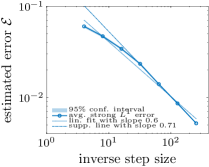
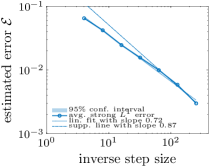
Refer to caption
(a) Correlation length ρ=0.01𝜌0.01\rho=0.01.
Refer to caption
(b) Correlation length ρ=0.05𝜌0.05\rho=0.05.
Refer to caption
(c) Correlation length ρ=0.1𝜌0.1\rho=0.1.
Fig. 7: Convergence of the finite volume approximation for different correlation length ρ𝜌\rho of the Matérn covariance kernel. The error estimation is based on 202020 samples.

4.4 Pathwise convergence study

In this section, we investigate the strong error of the jump-adapted and wave cell finite volume method when computing the stochastic Burgers equation (19bi). In the experiments described in Sections 4.4.1 and 4.4.2, we consider specific jump coefficients, which have the form described in (19au). Afterwards, in Section 4.4.3, we present experiments demonstrating the ability of the wave cell finite volume method. Therefore, we consider a stochastic jump coefficient without the Gaussian random field part, i.e., having the simpler form a(ω,x)=a¯(x)+P(ω,x)𝑎𝜔𝑥¯𝑎𝑥𝑃𝜔𝑥a(\omega,x)=\bar{a}(x)+P(\omega,x). For the convergence study, we consider both the strong L1superscript𝐿1L^{1}-error and the strong L2superscript𝐿2L^{2}-error, i.e.,

(19bp) (ω)\MT@delim@Auto\norm@staruΔref(ω,,T)uΔ(ω,,T)L(𝕏).𝜔\MT@delim@Auto\norm@starsubscriptsuperscript𝑢refΔ𝜔𝑇subscript𝑢Δsubscript𝜔𝑇superscript𝐿𝕏\mathcal{E}(\omega)\coloneqq\MT@delim@Auto\norm@star{u^{\text{ref}}_{\Delta}(\omega,\cdot,T)-u_{\Delta}(\omega,\cdot,T)}_{L^{\star}(\mathbb{X})}.

Here, uΔrefsubscriptsuperscript𝑢refΔu^{\text{ref}}_{\Delta} is a numerical reference solution computed on a finer grid, uΔsubscript𝑢Δu_{\Delta} is the considered approximation and \MT@delim@Auto\norm@starL(𝕏)\MT@delim@Auto\norm@star{\cdot}_{L^{\star}(\mathbb{X})} denotes either the L1(𝕏)superscript𝐿1𝕏L^{1}(\mathbb{X}) or the L2(𝕏)superscript𝐿2𝕏L^{2}(\mathbb{X}) norm.

4.4.1 Alternating jump field with exponential Gaussian random field

In this first experiment, we consider a Gaussian random field W𝑊W with the Matérn covariance operator (19bj) with a smoothness parameter ν=12𝜈12\nu=\frac{1}{2}. The jump field P(ω,x)𝑃𝜔𝑥P(\omega,x) has τPoi(5)+1similar-to𝜏𝑃𝑜𝑖51\tau\sim Poi(5)+1 jumps, which are located at the jump locations χi𝒰(𝒟)similar-tosubscript𝜒𝑖𝒰𝒟\chi_{i}\sim\mathcal{U}(\mathcal{D}). The jump heights Pisubscript𝑃𝑖P_{i} corresponding to the partition, are given by

(19bq) Pi{𝒰([14,34])for i odd,𝒰([54,74])for i even.similar-tosubscript𝑃𝑖cases𝒰1434for 𝑖 odd𝒰5474for 𝑖 even\displaystyle P_{i}\sim\begin{cases}\mathcal{U}([\frac{1}{4},\frac{3}{4}])&\text{for }i\text{ odd},\\ \mathcal{U}([\frac{5}{4},\frac{7}{4}])&\text{for }i\text{ even}.\end{cases}

To illustrate this coefficient, Figure 8 shows two realizations of the coefficient. One can see that the occurring jumps are relatively small compared to the variation of the Gaussian random field, which is influenced by the small smoothness parameter ν𝜈\nu, the variance σ2superscript𝜎2\sigma^{2} and the correlation length ρ𝜌\rho.

Refer to caption
Refer to caption
Fig. 8: Two samples of the alternating jump field with an exponential Gaussian random field.

In Figure 9, the pathwise L1superscript𝐿1L^{1}- and L2superscript𝐿2L^{2}-error are shown for 505050 samples. The corresponding reference solutions were computed with the wave cell finite volume method using a grid with approximately 444 times as many discretization points. One can see that the difference of the methods in not significant and that the order of convergence is similar. Since the distance between the jumps is quiet large on average, the discontinuities are already resolved on relatively coarse discretizations. Thus, the different in the discretizations has no significant effect and the presented behaviour is exactly, what we would expect.
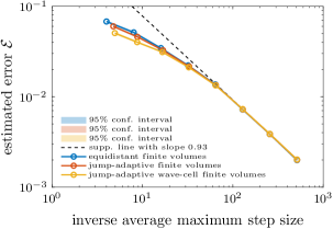
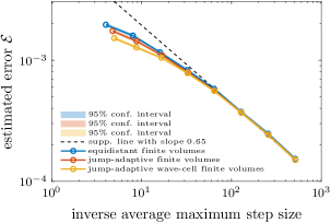
Refer to caption
(a) Pathwise L1superscript𝐿1L^{1} error.
Refer to caption
(b) Pathwise L2superscript𝐿2L^{2} error.
Fig. 9: Strong error for the alternating jump field with exponential Gaussian random field. The error estimation is based on 505050 samples.

4.4.2 Poisson jump field with squared-exponential Gaussian random field

In this experiment, we consider a similar jump field as in Section 4.4.1. The considered jump field P𝑃P has τPoi(5)+1similar-to𝜏𝑃𝑜𝑖51\tau\sim Poi(5)+1 jumps at jump positions χi𝒰(𝒟)similar-tosubscript𝜒𝑖𝒰𝒟\chi_{i}\sim\mathcal{U}(\mathcal{D}). The corresponding jump heights are PiPoi(5)+1similar-tosubscript𝑃𝑖𝑃𝑜𝑖51P_{i}\sim Poi(5)+1 distributed. This leads to a significant difference in the jump field, since the jump heights are not globally bounded. We additively combine this random jump field with a squared-exponential Gaussian random field, i.e., the Matérn covariance kernel (19bj) having a smoothness parameter of ν=𝜈\nu=\infty.

Two samples of this coefficient are shown in Figure 10. Note that, in contrast to the previous random field, the jumps are higher and have a more significant effect on the sample compared to the variation of the Gaussian part. Also, let us mention that this coefficient is more likely to have larger values than the random field presented in the previous subsection.
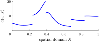
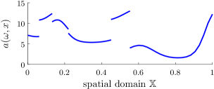
Refer to caption
Refer to caption
Fig. 10: Two realizations of the Poisson jump field with squared-exponential Gaussian random field.

The pathwise L1superscript𝐿1L^{1}- and L2superscript𝐿2L^{2}-error are shown in Figure 11. The convergence behaviour and the absolute error are again very similar, which is as expected, since the jumps are resolved on relatively coarse grids. However, we note a slightly higher convergence rate for both adapted discretization methods. This is not surprising, since the heights of the standing shock profiles resulting from the discontinuities in the flux function are better approximated with the adapted methods.
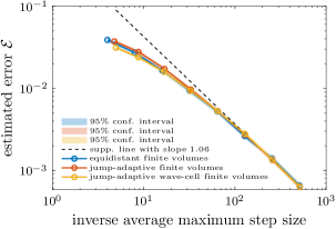
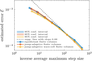
Refer to caption
(a) Pathwise L1superscript𝐿1L^{1} error.
Refer to caption
(b) Pathwise L2superscript𝐿2L^{2} error.
Fig. 11: Strong error for the Poisson jump field with squared-exponential Gaussian random field estimated with 505050 samples.

4.4.3 Jump field with random inclusions

In this last experiment, we demonstrate the ability of the wave cell finite volume discretization. Therefore, we consider the following stochastic jump coefficient having random inclusions: Let τPoi(10)+1similar-to𝜏𝑃𝑜𝑖101\tau\sim Poi(10)+1 denote the number of inclusions with positions χi𝒰(𝒟)similar-tosubscript𝜒𝑖𝒰𝒟\chi_{i}\sim\mathcal{U}(\mathcal{D}). The corresponding inclusion sizes are given by δi𝒰([105,103])similar-tosubscript𝛿𝑖𝒰superscript105superscript103\delta_{i}\sim\mathcal{U}([10^{-5},10^{-3}]) and the heights of the inclusions are given by

(19br) Hk{Poi(30)for k=0,1ξ,ξPoi(30)for k=1.similar-tosubscript𝐻𝑘cases𝑃𝑜𝑖30for 𝑘0similar-to1𝜉𝜉𝑃𝑜𝑖30for 𝑘1\displaystyle H_{k}\sim\begin{cases}Poi(30)&\text{for }k=0,\\ \frac{1}{\xi},\xi\sim Poi(30)&\text{for }k=1.\end{cases}

Let now 𝒟𝒟\mathfrak{I}\subset\mathcal{D} denote the union of all inclusion. We define the jump field with random inclusions as

(19bs) a(ω,x)={Hkfor x,1otherwise,𝑎𝜔𝑥casessubscript𝐻𝑘for 𝑥1otherwise,\displaystyle a(\omega,x)=\begin{cases}H_{k}&\text{for }x\in\mathfrak{I},\\ 1&\text{otherwise,}\end{cases}

where kB(1,12)similar-to𝑘𝐵112k\sim B(1,\frac{1}{2}) is a Bernoulli-1212\frac{1}{2}-distributed random variable, defining whether the inclusion height is given by H1subscript𝐻1H_{1} or by H2subscript𝐻2H_{2}.

The random field is illustrated in Figure 12, where two samples of the coefficient are shown. Note, the inclusions are marked with a circle to increase the visibility. Also, we see that the character of the random field is very different to the previous ones, since no Gaussian field is involved and thus the coefficient does not vary away from the jumps. However, due to the small size of the inclusions, this coefficient is promising to demonstrate the qualitative difference between the proposed meshing methods.
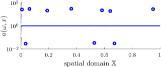
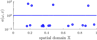
Refer to caption
Refer to caption
Fig. 12: Two realizations of the jump field with random inclusions.

In Figure 13, we can see the performance of the different discretization methods measured by the strong L1superscript𝐿1L^{1} and L2superscript𝐿2L^{2} error for 100100100 samples. While the adapted discretizations are converging with a similar rate, the standard finite volume method does not seem to converge at all or at a very low convergence rate. This behaviour is what one would expect for this jump coefficient and the standard finite volume method: Due to the small size of the inclusions, the standard finite volume scheme does not resolve the discontinuities in the flux function. Thus, when refining the spatial step size, the standard finite volume discretization needs a much finer resolution of the grid to resolve the discontinuities than the adaptive discretization schemes. Note, asymptotically, we expect all three discretization schemes to converge with the same convergence rate. We also note the better error constant in the wave cell finite volume method compared to the jump-adapted finite volume method. This behaviour can be explained by the better approximation of the standing wave profiles resulting from the discontinuities of the flux function.
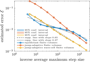
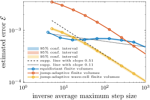
Refer to caption
(a) Pathwise L1superscript𝐿1L^{1} error.
Refer to caption
(b) Pathwise L2superscript𝐿2L^{2} error.
Fig. 13: Strong error for the stochastic jump field with random inclusions based on 100100100 samples.

Declaration of interest

None.

Acknowledgement

The research leading to these results has received funding from the German Research Foundation (Deutsche Forschungsgemeinschaft, DFG) under Germany’s Excellence Strategy EXC-2075 390740016 at the University of Stuttgart and it is gratefully acknowledged.

References

  • [1] Rémi Abgrall and Siddharta Mishra “Uncertainty quantification for hyperbolic systems of conservation laws” In Handbook of Numerical Analysis 18 Elsevier, 2017, pp. 507–544
  • [2] Adimurthi, Jérôme Jaffré and G.. Gowda “Godunov-Type Methods for Conservation Laws with a Flux Function Discontinuous in Space” In SIAM Journal on Numerical Analysis 42.1 Society for IndustrialApplied Mathematics, 2005, pp. 179–208 URL: http://www.jstor.org/stable/4101131
  • [3] C.. Aliprantis and K.. Border “Infinite Dimensional Analysis” Springer–Verlag, Berlin, Heidelberg, 2006
  • [4] Boris Andreianov, Konstantin Brenner and Clément Cancès “Approximating the vanishing capillarity limit of two-phase flow in multi-dimensional heterogeneous porous medium” In ZAMM – Journal of Applied Mathematics and Mechanics / Zeitschrift für Angewandte Mathematik und Mechanik 94.7-8 Wiley Online Library, 2014, pp. 655–667
  • [5] Boris Andreianov, Paola Goatin and Nicolas Seguin “Finite volume schemes for locally constrained conservation laws” In Numerische Mathematik 115.4 Springer, 2010, pp. 609–645
  • [6] Boris Andreianov, Kenneth H. Karlsen and Nils H. Risebro “A theory of L1superscript𝐿1{L}^{1}–dissipative solvers for scalar conservation laws with discontinuous flux” In Archive for Rational Mechanics and Analysis 201.1 Springer, 2011, pp. 27–86
  • [7] David Applebaum “Lévy processes and stochastic calculus” Cambridge university press, 2009
  • [8] Emmanuel Audusse and Benoît Perthame “Uniqueness for scalar conservation laws with discontinuous flux via adapted entropies” In Proceedings of the Royal Society of Edinburgh Section A: Mathematics 135.2 Royal Society of Edinburgh Scotland Foundation, 2005, pp. 253–265
  • [9] Paolo Baiti and Helge K. Jenssen “Well-Posedness for a Class of 2×\times2 Conservation Laws with Lsuperscript𝐿{L}^{\infty} Data” In Journal of Differential Equations 140.1 Elsevier, 1997, pp. 161–185
  • [10] Andrea Barth and Andreas Stein “A stochastic transport problem with Lévy noise: Fully discrete numerical approximation” Preprint arXiv:1910.14657 In arXiv, 2019
  • [11] Andrea Barth and Andreas Stein “A study of elliptic partial differential equations with jump diffusion coefficients” In Journal on Uncertainty Quantification 6.4 SIAM/ASA, 2018, pp. 1707–1743
  • [12] Andrea Barth and Andreas Stein “Numerical analysis for time-dependent advection-diffusion problems with random discontinuous coefficients” Submitted In Stochastics and Partial Differential Equations: Analysis and Computations, 2020
  • [13] Caroline Bauzet, Guy Vallet and Petra Wittbold “The Cauchy problem for conservation laws with a multiplicative stochastic perturbation” In Journal of Hyperbolic Differential Equations 9.04 World Scientific, 2012, pp. 661–709
  • [14] Imran H. Biswas, Kenneth H. Karlsen and Ananta K. Majee “Conservation laws driven by Lévy white noise” In Journal of Hyperbolic Differential Equations 12.03 World Scientific, 2015, pp. 581–654
  • [15] François Bouchut and Benoıt Perthame “Kružkov’s estimates for scalar conservation laws revisited” In Transactions of the American Mathematical Society 350.7, 1998, pp. 2847–2870
  • [16] Miroslav Bulíček, Piotr Gwiazda, Josef Málek and Agnieszka Świerczewska-Gwiazda “On scalar hyperbolic conservation laws with a discontinuous flux” In Mathematical Models and Methods in Applied Sciences 21.01 World Scientific, 2011, pp. 89–113
  • [17] Raimund Bürger, Ilja Kröker and Christian Rohde “A hybrid stochastic Galerkin method for uncertainty quantification applied to a conservation law modelling a clarifier-thickener unit” In ZAMM – Journal of Applied Mathematics and Mechanics / Zeitschrift für Angewandte Mathematik und Mechanik 94.10 Wiley Online Library, 2014, pp. 793–817
  • [18] Raimund Bürger, Kenneth H. Karlsen, Nils Henrik Risebro and John D. Towers “Well-posedness in BV t and convergence of a difference scheme for continuous sedimentation in ideal clarifier-thickener units” In Numerische Mathematik 97.1 Springer, 2004, pp. 25–65
  • [19] Gui-Qiang Chen, Nadine Even and Christian Klingenberg “Hyperbolic conservation laws with discontinuous fluxes and hydrodynamic limit for particle systems” In Journal of Differential Equations 245.11 Elsevier, 2008, pp. 3095–3126
  • [20] Giuseppe Maria Coclite, Mauro Garavello and Benedetto Piccoli “Traffic flow on a road network” In SIAM Journal on Mathematical Analysis 36.6 SIAM, 2005, pp. 1862–1886
  • [21] Constantine M. Dafermos “Hyperbolic conservation laws in continuum physics” Springer, 2000
  • [22] Jin Feng and David Nualart “Stochastic scalar conservation laws” In Journal of Functional Analysis 255.2 Elsevier, 2008, pp. 313–373
  • [23] Abebe Geletu “Introduction to topological spaces and set-valued maps (Lecture notes)” Institute of Mathematics. Department of Operations ResearchStochastics, 2006
  • [24] Shyam S. Ghoshal, Animesh Jana and John D. Towers “Convergence of a Godunov scheme to an Audusse-Perthame adapted entropy solution for conservation laws with BV spatial flux” Preprint arXiv:2003.10321 In arXiv, 2020
  • [25] Shyam Sundar Ghoshal, Rajib Dutta and G.. Veerappa Gowda “Existence and nonexistence of TV bounds for scalar conservation laws with discontinuous flux” In Communications on Pure and Applied Mathematics 64.1 Wiley Online Library, 2011, pp. 84–115
  • [26] Tore Gimse and Nils H. Risebro “Solution of the Cauchy problem for a conservation law with a discontinuous flux function” In SIAM Journal on Mathematical Analysis 23.3 SIAM, 1992, pp. 635–648
  • [27] Martina Hofmanova “Scalar conservation laws with rough flux and stochastic forcing” In Stochastics and Partial Differential Equations: Analysis and Computations 4.3 Springer, 2016, pp. 635–690
  • [28] Helge Holden and Nils H. Risebro “Conservation laws with a random source” In Applied Mathematics and Optimization 36.2 Springer, 1997, pp. 229–241
  • [29] Jérôme Jaffré “Numerical calculation of the flux across an interface between two rock types of a porous medium for a two-phase flow” Citeseer, 1996
  • [30] Kenneth Hvistendahl Karlsen and Erlend Briseid Storrøsten “On stochastic conservation laws and Malliavin calculus” In Journal of Functional Analysis 272.02 Elsevier, 2017, pp. 421–497
  • [31] Sato Ken-Iti “Lévy processes and infinitely divisible distributions” Cambridge university press, 1999
  • [32] Jong Uhn Kim “On a stochastic scalar conservation law” In Indiana University Mathematics Journal JSTOR, 2003, pp. 227–256
  • [33] Ujjwal Koley, Nils Henrik Risebro, Christoph Schwab and Franziska Weber “A multilevel Monte Carlo finite difference method for random scalar degenerate convection–diffusion equations” In Journal of Hyperbolic Differential Equations 14.03 World Scientific, 2017, pp. 415–454
  • [34] Stanislav N. Kružkov “First order quasilinear equations in several independent variables” In Mathematics of the USSR-Sbornik 10.2 IOP Publishing, 1970, pp. 217
  • [35] Randall J. LeVeque “Numerical methods for conservation laws” Springer, 1992
  • [36] Pierre-Louis Lions, Benoît Perthame and Panagiotis E. Souganidis “Scalar conservation laws with rough (stochastic) fluxes” In Stochastic Partial Differential Equations: Analysis and Computations 1.4 Springer, 2013, pp. 664–686
  • [37] Pierre-Louis Lions, Benoît Perthame and Panagiotis E. Souganidis “Scalar conservation laws with rough (stochastic) fluxes: the spatially dependent case” In Stochastic Partial Differential Equations: Analysis and Computations 2.4 Springer, 2014, pp. 517–538
  • [38] Siddhartha Mishra and Ch Schwab “Sparse tensor multi-level Monte Carlo finite volume methods for hyperbolic conservation laws with random initial data” In Mathematics of Computation 81.280, 2012, pp. 1979–2018
  • [39] Siddhartha Mishra, Ch Schwab and Jonas Sukys “Multilevel Monte Carlo finite volume methods for shallow water equations with uncertain topography in multi-dimensions” In SIAM Journal on Scientific Computing 34.6 SIAM, 2012, pp. B761–B784
  • [40] Siddhartha Mishra, Ch Schwab and Jonas Šukys “Multi-level Monte Carlo finite volume methods for nonlinear systems of conservation laws in multi-dimensions” In Journal of Computational Physics 231.8 Elsevier, 2012, pp. 3365–3388
  • [41] Siddhartha Mishra, Nils Henrik Risebro, Christoph Schwab and Svetlana Tokareva “Numerical solution of scalar conservation laws with random flux functions” In SIAM/ASA Journal on Uncertainty Quantification 4.1 SIAM, 2016, pp. 552–591
  • [42] Benoît Perthame, Nicolas Seguin and Magali Tournus “A simple derivation of BV bounds for inhomogeneous relaxation systems” Preprint arXiv:1404.1604 In arXiv, 2014
  • [43] Gaël Poëtte, Bruno Després and Didier Lucor “Uncertainty quantification for systems of conservation laws” In Journal of Computational Physics 228.7 Elsevier, 2009, pp. 2443–2467
  • [44] Nils Henrik Risebro, Christoph Schwab and Franziska Weber “Multilevel Monte Carlo front-tracking for random scalar conservation laws” In BIT Numerical Mathematics 56.1 Springer, 2016, pp. 263–292
  • [45] John D. Towers “An existence result for conservation laws having BV spatial flux heterogeneities - without concavity” In Journal of Differential Equations 269, 2020, pp. 5754–5764
  • [46] John D. Towers “Convergence of a difference scheme for conservation laws with a discontinuous flux” In SIAM Journal on Numerical Analysis 38.2 SIAM, 2000, pp. 681–698
  • [47] John D. Towers “Convergence of the Godunov scheme for a scalar conservation law with time and space discontinuities” In Journal of Hyperbolic Differential Equations 15.02 World Scientific, 2018, pp. 175–190
  • [48] Julie Tryoen, O. Maiître and Alexandre Ern “Adaptive anisotropic spectral stochastic methods for uncertain scalar conservation laws” In SIAM Journal on Scientific Computing 34.5 SIAM, 2012, pp. A2459–A2481
  • [49] Christopher K.. Williams and Carl E. Rasmussen “Gaussian processes for machine learning” MIT press Cambridge, MA, 2006