Distribution-Free Prediction Bands for Multivariate Functional Time Series: an Application to the Italian Gas Market

Abstract

Uncertainty quantification in forecasting represents a topic of great importance in energy trading, as understanding the status of the energy market would enable traders to directly evaluate the impact of their own offers/bids. To this end, we propose a scalable procedure that outputs closed-form simultaneous prediction bands for multivariate functional response variables in a time series setting, which is able to guarantee performance bounds in terms of unconditional coverage and asymptotic exactness, both under some conditions. After evaluating its performance on synthetic data, the method is used to build multivariate prediction bands for daily demand and offer curves in the Italian gas market.

[unipd]organization=Department of Statistical Sciences, University of Padova,country=Italy [JRC]organization=now at European Commission, Joint Research Centre (JRC),city=Ispra, state=(VA), country=Italy [MOX]organization=MOX - Department of Mathematics, Politecnico di Milano,country=Italy

1 Introduction

The emergence of a new regulatory framework for electricity and gas markets, particularly in Italy, has presented significant challenges to industry players. Following decades of state monopoly, either de iure and de facto, the market has undergone privatization, leading to unprecedented challenges for producers, brokers, and utilities. Accurate forecasting of exchange quantities and market prices has become essential for strategic and tactical planning related to energy production, storage, and trading. Given the unpredictable nature of markets, quantifying uncertainties has become a crucial factor. Reliable assessments of prediction uncertainties offer invaluable insights into risk management and represent the foundation of any effective hedging strategy in trading.

Forecasts, though, should not only be constrained to spot quantities and prices: the market is a dynamic object, and it is crucial to be able to understand not only its behaviour at equilibrium but also its ”shape” in terms of position and slope of its demand and offer curves, allowing traders to evaluate the possible effect of their offers/bids on the market. These specific issues have triggered cutting edge research, in the Functional Data Analysis realm. Works like [1] alongside [2] represent some recent contribution in the field, containing also a thorough representation of the history of price and demand forecasting in the electricity and gas markets.

Functional Data Analysis, or FDA [3, 4, 5, 6] is the specific branch of statistics that deals with continuous phenomena over a spatial or a temporal domain (e.g. a trajectory, a surface or a demand/offer curve).

Expanding on [1], [7] adds uncertainty quantification to the framework presented for the gas market. As previously said though, these bands have no finite-sample coverage guarantee. The aim of our application test case is thus to show how our methodological proposal may provide more reliable information in terms of prediction uncertainty to energy traders.

For instance, when dealing with continuous phenomena over a spatial or a temporal domain (e.g. a trajectory, a surface or a demand/offer curve) instead of using standard scalar statistics and working on a statistical summary of these objects, a practitioner may decide to turn to Functional Data Analysis (FDA)[3, 4, 5, 6].

A field of research with very promising applications in FDA is Functional Time Series (FTS), namely the study of methods and the development of applications to deal with functional data characterised by some kind of temporal dependency. The interested reader may refer to [8] for a review of the theoretical underpinnings and some definitions on the field. The main focus of FTS, as testified by the very rich outstanding literature, has been the issue of one-step ahead forecasting. Among the many contributions that may be found in the literature, [9] provides a review of some of the work on point prediction for FTS using autoregressive models, Ferraty et al. [10], Ferraty and Vieu [11] present nonparametric methods and [1] presents an extension for the forecasting of FTS with constraints. On a slightly different line of reasoning [12] proposes a method based on dimensionality reduction via weighted functional principal component and weighted functional partial least squares regression while [13] proposes a vector error-correcting model, still based on dimensionality reduction of functional data.

The great majority of the presented work in FTS forecasting focuses on point predictions: the issue of providing quantification of uncertainty is usually addressed using extensions of the Bootstrap to non $i.i.d$ cases (see e.g. [14], which also provides a good introduction to the field, as well as [7] where a remarkable extension to the constrained FTS case is presented). Bootstrap-based methods, though, are shown to have relatively weak finite-sample properties, and are of course very computationally intensive.

On a related note, many research efforts have been performed to create forecasting methods that achieve provable theoretical properties even under very minimal assumptions. One of the most general in this regard is Conformal Prediction [15], a method invented to provide prediction intervals to Support Vector Machines [16]. The fundamental advantage of Conformal methods over other ways of generating forecasts is the fact that, to provide valid prediction sets - i.e. prediction sets ensuring a coverage no less than the nominal confidence level -, it only requires the data to be exchangeable, thus providing an extremely flexible method to be used in statistics. Conformal prediction has now been used and extended to solve many problems in the statistical practice: the interested reader can find an introduction and an updated state of the art in [17]. Another additional methodological advancement of Conformal Prediction is its extension to the generation of prediction bands for functional data: [18] in the case of identically distributed univariate functional data, while [19] deals with the multivariate, regression case. Moving away from the requirements of data exchangeability, a relatively new contribution by [20] shows an extension of Conformal methods to time dependent data.

The aim of the present work is explictly tackle the need of uncertainty quantification in the prediction of gas supply and demand curves, by reaching a synthesis between two rich and ebullient fields of methodological literature (namely, set forecasting for (multivariate) FTS and finite-sample valid distribution-free prediction) by proposing distribution-free prediction bands for multivariate functional time series guaranteeing finite-sample performance bounds in terms of coverage and asymptotic exactness, i.e. coverage asymptotically equal to the nominal confidence level. The paper is structured as follows: Section 2 presents the proposed method and its theoretical underpinnings in detail, while in Section 3 and 3.1 we present a simulation study to assess the properties of the method and its results. The application is presented in Section 4 while Section 5 presents conclusions and draws further developments.

2 Methods

Let $\boldsymbol{Z}_{1},\dots,\boldsymbol{Z}_{T}$ be a time series such that $\boldsymbol{Z}_{t}=(\boldsymbol{X}_{t},\boldsymbol{Y}_{t})$ consists of a set of covariates $\boldsymbol{X}_{t}$ and a multivariate functional response variable $\boldsymbol{Y}_{t}$, $\forall t=1,\dots,T$. Let $\boldsymbol{Y}_{t}=(Y_{t1},Y_{t2},\dots,Y_{tp})$ be a multivariate random function where its $j$-th component $Y_{tj}$ ($j=1,\dots,p$) is a random function which takes values in $L^{\infty}(\mathcal{Q}_{j})$, that is the family of limited functions $y:\mathcal{Q}_{j}\rightarrow\mathbb{R}$ with $\mathcal{Q}_{j}$ closed and bounded subset of $\mathbb{R}^{d_{j}}$, $d_{j}\in\mathbb{N}_{>0}$. For simplicity, later in the discussion we will use $\prod_{j=1}^{p}L^{\infty}(\mathcal{Q}_{j})$ to indicate the space $L^{\infty}(\mathcal{Q}_{1})\times\dots\times L^{\infty}(\mathcal{Q}_{p})$ in which $\boldsymbol{Y}_{t}$ takes values. The framework considered is very general since it includes the case of univariate functional response variable (when $p=1$) as a special case, but it also allows the $p>1$ domains $\mathcal{Q}_{j}$ and images of $Y_{tj}$ to be greatly different when $j$ changes. $\boldsymbol{X}_{t}=(X_{t1},X_{t2},\dots,X_{tp})$ is a set of covariates where its $j$-th element $X_{tj}$ is made up of the covariates related to $Y_{tj}$. Specifically, $X_{tj}$ belongs to a measurable space and it can be conveniently represented as a set of covariates itself: differently from the notation traditionally used, $X_{tj}$ contains the lagged functional response variable (e.g., $Y_{t-1,j},Y_{t-2,j}$, etc.), in addition to possible external predictors (which can be, for example, scalar or functional covariates). As regards the notation, it is important to notice that two components of $\boldsymbol{Y}_{t}$ ($Y_{t1}$ and $Y_{t2}$ for example) may share some (or even all) the covariates, and so a unique set of covariates $X_{t}$ could be used instead of $\boldsymbol{X}_{t}=(X_{t1},X_{t2},\dots,X_{tp})$. However, we will use the previously mentioned notation to emphasize the fact that different sets of covariates can be used to predict the $p$ random functions $Y_{t1},\dots,Y_{tp}$. Let $\mu^{j}(x_{tj})=\mathbb{E}(Y_{tj}|X_{tj}=x_{tj})$ be the regression map for the $j$-th component evaluated at $x_{tj}$, and similarly let us define the scalar quantity $[\mu^{j}(x_{tj})](q)=\mathbb{E}(Y_{tj}(q)|X_{tj}=x_{tj})$.

Our aim is to introduce a procedure able to create simultaneous prediction sets for $\boldsymbol{Y}_{T+1}$ (i.e. prediction sets holding for the multivariate random function $\boldsymbol{Y}_{T+1}$ globally, and not only for its $j$-th component $Y_{T+1,j}$) based on the information provided by $\boldsymbol{Z}_{1},\dots,\boldsymbol{Z}_{T}$ and by $\boldsymbol{X}_{T+1}$ and ensuring performance bounds in terms of unconditional coverage. By formally defining a prediction set for $\boldsymbol{Y}_{T+1}$ based on $\boldsymbol{Z}_{1},\dots,\boldsymbol{Z}_{T}$ and $\boldsymbol{X}_{T+1}$ as $\mathcal{C}_{T,1-\alpha}\left(\boldsymbol{X}_{T+1}\right)$ for any significance level $\alpha\in(0,1)$, the purpose is to obtain prediction sets whose unconditional coverage $\mathbb{P}\left(\boldsymbol{Y}_{T+1}\in\mathcal{C}_{T,1-\alpha}\left(\boldsymbol{X}_{T+1}\right)\right)$ is close to the nominal confidence level $1-\alpha$ under mild conditions on the data generating process. Within the possible kinds of prediction set, the specific aim, moreover, is to find a prediction set having a particular shape, known as multivariate functional prediction band [19], which is defined as

$$\left\{\boldsymbol{y}=(y_{1},\dots,y_{p})\in\prod_{j=1}^{p}L^{\infty}(\mathcal{Q}_{j}):y_{j}(q)\in B_{j}(q),\quad\forall j\in 1,\dots,p,\quad\forall q\in\mathcal{Q}_{j},\right\},$$

with $B_{j}(q)$ interval $\forall j,q$. We focus on multivariate functional prediction bands because they are conceptually simple and they can be visualized in parallel coordinates [21]. More details on the topic can be found in Diquigiovanni et al. [18].

Moving from the literature on inference via permutations [see, e.g., 22, 23, 24] and on Conformal Prediction [see, e.g., 15, 25, 17], we present a modification of the Conformal inference able to account for time series dependence. Intuitively, the idea is to generalize the Conformal approach traditionally used when the regression pairs $\boldsymbol{Z}_{1},\dots,\boldsymbol{Z}_{T+1}$ are i.i.d. by randomizing blocks of observations. Specifically, we extend the non-overlapping blocking scheme proposed by Chernozhukov et al. [20] to the Semi-Off-Line Inductive (simply known as Split) framework. This extension is mentioned as possible in Chernozhukov et al. [20], nevertheless to the best of our knowledge it has never been formally built - or even taken into account - in the literature. In light of this, first of all the procedure we built is presented, then its logic is explained.

Let $m,l$ be two strictly positive integers such that $T=m+l$, and let us define $\mathcal{I}_{1}$ and $\mathcal{I}_{2}$ as two sets of size $m$ and $l$ respectively such that $\mathcal{I}_{1}\cup\mathcal{I}_{2}=\{1,\dots,T\}$, $\mathcal{I}_{1}\cap\mathcal{I}_{2}=\emptyset$. Let $\boldsymbol{z}_{1},\dots,\boldsymbol{z}_{T}$ be realizations of $\boldsymbol{Z}_{1},\dots,\boldsymbol{Z}_{T}$, with $\{\boldsymbol{z}_{h}:h\in\mathcal{I}_{1}\}$ denoting the training set of size $m$ and $\{\boldsymbol{z}_{h}:h\in\mathcal{I}_{2}\}$ denoting the calibration set of size $l$, and let $b\in\{1,\dots,l+1\}$ be a value such that $(l+1)/b$ is an integer. In accordance with the Conformal Prediction framework, let us also define any measurable function $A(\{\boldsymbol{z}_{h}:h\in\mathcal{I}_{1}\},\boldsymbol{z})$ which takes values in $\bar{\mathbb{R}}$ as nonconformity measure. As suggested by the name, the purpose of the nonconformity measure is to score how different the generic element $\boldsymbol{z}$ is from the elements of the training set: for example, in the traditional non-functional regression framework in which the response variable is scalar and the set of covariates is a vector, a popular choice of nonconformity measure is the absolute value of the regression residual obtained by fitting the regression algorithm on the training set. For any given value of $b$, it is therefore possible to define the collection of $(l+1)/b$ index permutations $\Pi=\{\pi_{i}:1\leq i\leq(l+1)/b\}$, whose element $\pi_{i}:\{1,\dots,l+1\}\longrightarrow\{1,\dots,l+1\}$ is the bijective function defined as:

$$\pi_{i}(t)=\left\{\begin{array}[]{ll}t+(i-1)b&\text{ if }1\leq t\leq l-(i-1)b+1\\ t+(i-1)b-l-1&\text{ if }l-(i-1)b+2\leq t\leq l+1.\end{array}\right.$$

The permutation scheme $\Pi$ is an algebraic group containing the identity element (as $\pi_{1}(t)=t$ $\forall t\in\{1,\dots,l+1\}$) which naturally induces the set of scalar values $\mathcal{D}_{\Pi}=\{\pi_{i}(l+1):1\leq i\leq(l+1)/b\}\subseteq\{1,\dots,l+1\}$, which is the set of integers used to identify the observations for which the nonconformity scores will be calculated.

The prediction set for $\boldsymbol{Y}_{T+1}$ (which is a multivariate prediction band or not depending on the choice of the nonconformity measure) is therefore defined as

$$\mathcal{C}_{T,1-\alpha}\left(\boldsymbol{x}_{T+1}\right):=\left\{\boldsymbol{y}\in\prod_{j=1}^{p}L^{\infty}(\mathcal{Q}_{j}):\delta_{\boldsymbol{y}}>\alpha\right\},$$

with

$$\delta_{\boldsymbol{y}}:=\frac{\left|\left\{d\in\mathcal{D}_{\Pi}:R_{\omega_{d}}\geq R_{T+1}\right\}\right|}{|\mathcal{D}_{\Pi}|},$$

$|\mathcal{D}_{\Pi}|=(l+1)/b$, $\omega_{d}$ the $d$th smallest value in the set $\mathcal{I}_{2}\cup\{T+1\}$ and nonconformity scores $R_{\omega_{d}}:=A(\{\boldsymbol{z}_{h}:h\in\mathcal{I}_{1}\},\boldsymbol{z}_{\omega_{d}})$, $R_{T+1}:=A(\{\boldsymbol{z}_{h}:h\in\mathcal{I}_{1}\},\boldsymbol{z}_{T+1})$, where $\boldsymbol{z}_{T+1}=\left(\boldsymbol{x}_{T+1},\boldsymbol{y}\right)$. Since $T+1$ is always included in $\{\omega_{d}:d\in\mathcal{D}_{\Pi}\}$ (being $l+1=\pi_{1}(l+1)$ and $\omega_{l+1}=T+1$), $\delta_{y}$ can be conveniently rewritten as

$$\delta_{\boldsymbol{y}}=\frac{1+\left|\left\{d\in\{\pi_{i}(l+1):2\leq i\leq(l+1)/b\}:R_{\omega_{d}}\geq R_{T+1}\right\}\right|}{|\mathcal{D}_{\Pi}|}.$$

Intuitively, the idea is the one introduced by Split Conformal Prediction: after randomly dividing the observed data into the training and calibration sets, the prediction set $\mathcal{C}_{T,1-\alpha}\left(\boldsymbol{x}_{T+1}\right)$ is defined as the set of all $\boldsymbol{y}\in\prod_{j=1}^{p}L^{\infty}(\mathcal{Q}_{j})$ such that $\left(\boldsymbol{x}_{T+1},\boldsymbol{y}\right)$ is similar - in terms of nonconformity measure $A$ - to the training set $\{\boldsymbol{z}_{h}:h\in\mathcal{I}_{1}\}$ compared to the conformity of the elements of the calibration set to the same training set. Differently from the Split Conformal Prediction framework, the permutation scheme here proposed randomizes the elements of the calibration set by considering blocks of observations of length $b$, and it computes the nonconformity scores for $(l+1)/b-1$ elements of the calibration set (one for each block) and for $\boldsymbol{z}_{T+1}$. In so doing, when $b$ increases the nonconformity scores are computed for observations more distant in time from each other (and so one is justified in expecting the dependence between the nonconformity scores to decrease under some conditions on the data generating process, a fundamental aspect as we will see shortly), but the number of nonconformity scores computed decreases. On the other hand, when $b=1$ the approach here proposed is equivalent to the Split Conformal approach, and the nonconformity scores are computed for each observation in the calibration set.

Regardless the value of $b$, the permutation scheme $\Pi$ guarantees that, if the regression pairs $\boldsymbol{Z}_{1},\dots,\boldsymbol{Z}_{T+1}$ are i.i.d. (or even exchangeable), the prediction sets obtained are finite-sample valid, i.e. $\mathbb{P}\left(\boldsymbol{Y}_{T+1}\in\mathcal{C}_{T,1-\alpha}\left(\boldsymbol{X}_{T+1}\right)\right)\geq 1-\alpha$ $\forall$ $T,\alpha\in(0,1)$, due to the fact that the nonconformity scores are exchangeable. The proof can be trivially obtained by generalizing the well-established result holding in the Split Conformal framework [15]. As in the Conformal setting, the result concerning the validity of the prediction sets induced by the permutation scheme $\Pi$ can be enriched by proving that, if the nonconformity scores have a continuous joint distribution, then $\mathbb{P}\left(\boldsymbol{Y}_{T+1}\in\mathcal{C}_{T,1-\alpha}\left(\boldsymbol{X}_{T+1}\right)\right)=1-\frac{\lfloor\alpha(l+1)/b\rfloor}{(l+1)/b}$ , i.e. the unconditional coverage is equal to an easy-to-compute value and it is not only greater than or equal to $1-\alpha$. Also in this case, the proof can be trivially obtained by generalizing an existing result concerning Conformal Prediction [see Theorem 1 of 18].

If the regression pairs are not exchangeable, as in our case, the aforementioned results do not hold. Nevertheless, two desirable properties can still be obtained under some conditions: finite-sample performance bounds in terms of unconditional coverage and asymptotic exactness (i.e. unconditional coverage asymptotically equal to the nominal confidence level $1-\alpha$). These results, which represent an extension of a result due to Chernozhukov et al. [20] to the Split framework, are reported in Theorem 2.1.

In order to introduce Theorem 2.1, let $A^{*}$ be an oracle nonconformity measure inducing oracle nonconformity score $R^{*}_{\omega_{d}}$, which is typically the population counterpart of $R_{\omega_{d}}$: for example, in the aforementioned non-functional regression setting, the oracle nonconformity score might be the magnitude of the error term. For notational simplicity, let us define $\bar{l}=|\mathcal{D}_{\Pi}|=(l+1)/b$ and let $\{\delta_{1\bar{l}},\delta_{2m},\gamma_{1\bar{l}},\gamma_{2m}\}$ be sequences of positive scalar values converging to 0 when $\bar{l},m\rightarrow 0$. Finally, let $\tilde{F}(a):=\frac{1}{\bar{l}}\sum_{d\in\mathcal{D}_{\Pi}}\mathbbm{1}\left\{R^{*}_{\omega_{d}}<a\right\}$ and $F(a)=P(R^{*}_{T+1}<a)$.

Theorem 2.1.

If

• $\sup_{a\in\mathbb{R}}|\tilde{F}(a)-F(a)|\leq\delta_{1\bar{l}}$ with probability $1-\gamma_{1\bar{l}}$,

• $\frac{1}{\bar{l}}\sum_{d\in\mathcal{D}_{\Pi}}\left[R_{\omega_{d}}-R^{*}_{\omega_{d}}\right]^{2}\leq\delta_{2m}^{2}$ with probability $1-\gamma_{2m}$,

• $|R_{T+1}-R^{*}_{T+1}|\leq\delta_{2m}$ with probability $1-\gamma_{2m}$,

• The probability density function of $R^{*}_{T+1}$ is bounded above by a constant $D$,

then

$$\left|\mathbb{P}\left(\boldsymbol{Y}_{T+1}\in\mathcal{C}_{T,1-\alpha}\left(\boldsymbol{X}_{T+1}\right)\right)-(1-\alpha)\right|\leq 6\delta_{1\bar{l}}+2\delta_{2m}+2D\left(\delta_{2m}+2\sqrt{\delta_{2m}}\right)+\gamma_{1\bar{l}}+\gamma_{2m}$$ (1)

$\forall$ $\alpha\in(0,1)$.

The first condition concerns the approximate ergodicity of $\tilde{F}(a)$ for $F(a)$, a condition which holds for strongly mixing time series using the permutation scheme $\Pi$ [20]. The remaining conditions mainly concern the relationship between the nonconformity scores and the oracle nonconformity scores: intuitively, $\delta_{2m}$ bounds the discrepancy between the nonconformity scores and their oracle counterparts. The proof of the Theorem mimics the proof of Theorem 2 in Chernozhukov et al. [20] if $\{\delta_{1n},\delta_{2n},\gamma_{1n},\gamma_{2n}\}$ are respectively replaced by $\{\delta_{1\bar{l}},\delta_{2m},\gamma_{1\bar{l}},\gamma_{2m}\}$. We thus cross-refer to Chernozhukov et al. [20] for details. Considering the Split framework of the manuscript, we require the four sequences $\{\delta_{1\bar{l}},\delta_{2m},\gamma_{1\bar{l}},\gamma_{2m}\}$ to depend on $m$ and $\bar{l}$ respectively according to their specific role: indeed, $R_{\omega_{d}}$ depends on the information provided by the training set, and so one is justified in requiring it to better approximate $R^{*}_{\omega_{d}}$ when the training set size $m$ increases. As a consequence, $\{\delta_{2m},\gamma_{2m}\}$ should depend on $m$. Conversely, the training set size does not affect $\tilde{F}(a)$ and $F(a)$ respectively since the training set does not affect the oracle nonconformity scores, and so the requirement is that the oracle nonconformity scores computed on the observations of the calibration set provide a proper approximation to $R^{*}_{T+1}$ when the calibration set size increases. In so doing, $\{\delta_{1\bar{l}},\gamma_{1\bar{l}}\}$ should depend on $\bar{l}$.

Theorem 2.1 provides, under some conditions, finite-sample performance bounds in terms of unconditional coverage regardless the value of $b$ and it guarantees that the prediction sets are asymptotically exact since the right side of Inequality (1) converges to 0 when $m,\bar{l}\rightarrow 0$. In view of this, the last, fundamental step in describing a strategy which can be used in practical applications is the definition of the nonconformity measure, a nontrivial issue in the functional setting. In view of this, we will consider the nonconformity measure proposed by [19]. This specific measure is particularly appealing since the permutation scheme $\Pi$ presented in the manuscript allows to determine whether a given value of $\boldsymbol{y}$ belongs or not to $\mathcal{C}_{T,1-\alpha}\left(\boldsymbol{x}_{T+1}\right)$ in a very simple way, but generally speaking (i.e. by considering a generic nonconformity measure) finding $\mathcal{C}_{T,1-\alpha}\left(\boldsymbol{x}_{T+1}\right)$ requires to evaluate the condition $\delta_{\boldsymbol{y}}>\alpha$ for every $\boldsymbol{y}$ belonging to the sample space, an unfeasible task given the infinite-dimensional nature of functional data. By using the nonconformity measure in [19], the prediction set can be instead found in a closed form and it is a multivariate functional prediction band, a key feature as stated before. Formally, the nonconformity measure considered induces the following nonconformity scores:

$$R_{\omega_{d}}= \sup_{j\in\{1,\dots,p\}}\left(\operatorname*{ess\,sup}_{q\in\mathcal{Q}_{j}}\left|\frac{y_{\omega_{d},j}(q)-[\hat{\mu}^{j}_{\mathcal{I}_{1}}(x_{\omega_{d},j})](q)}{s_{j,\mathcal{I}_{1}}(q)}\right|\right),\quad d\in\left\{\mathcal{D}_{\Pi}\setminus\left\{l+1\right\}\right\},$$ (2)

$$R_{T+1}= \sup_{j\in\{1,\dots,p\}}\left(\operatorname*{ess\,sup}_{q\in\mathcal{Q}_{j}}\left|\frac{y_{j}(q)-[\hat{\mu}^{j}_{\mathcal{I}_{1}}(x_{T+1,j})](q)}{s_{j,\mathcal{I}_{1}}(q)}\right|\right),$$

with $y_{j}$ the $j$-th component of $\boldsymbol{y}$, $[\hat{\mu}^{j}_{\mathcal{I}_{1}}(x_{\omega_{d},j})](q)$ estimate of $[\mu^{j}(x_{\omega_{d},j})](q)$ based on the training set $\{\boldsymbol{z}_{h}:h\in\mathcal{I}_{1}\}$, $s_{j,\mathcal{I}_{1}}$ the standard deviation function of the functional regression residuals of the observations belonging to the training set, i.e.:

$$s_{j,\mathcal{I}_{1}}(q):=\left(\sum_{h\in\mathcal{I}_{1}}\left(y_{hj}(q)-[\hat{\mu}^{j}_{\mathcal{I}_{1}}(x_{hj})](q)\right)^{2}\right)^{1/2}.$$ (3)

By considering this nonconformity measure, if $\alpha\in[b/(l+1),1)$ (which is the scenario we will consider hereafter because if $\alpha\in(0,b/(l+1))$ then $\mathcal{C}_{T,1-\alpha}\left(\boldsymbol{x}_{T+1}\right)=\prod_{j=1}^{p}L^{\infty}(\mathcal{Q}_{j})$ since $\delta_{\boldsymbol{y}}$ is always greater than or equal to $b/(l+1)$), then

$$\mathcal{C}_{T,1-\alpha}\left(\boldsymbol{x}_{T+1}\right):=\bigg{\{}\boldsymbol{y}\in\prod_{j=1}^{p}L^{\infty}(\mathcal{Q}_{j}):y_{j}(q)\in\big{[} [\hat{\mu}^{j}_{\mathcal{I}_{1}}(x_{T+1,j})](q)-k\cdot s_{j,\mathcal{I}_{1}}(q),$$

$$[\hat{\mu}^{j}_{\mathcal{I}_{1}}(x_{T+1,j})](q)+k\cdot s_{j,\mathcal{I}_{1}}(q)]$$

$$\forall j\in\{1,\dots,p\},\forall q\in\mathcal{Q}_{j}\bigg{\}},$$

with $k$ the $\lceil(l+1)(1-\alpha)/b\rceil$th smallest value in the set $\{R_{\omega_{d}}:d\in\left\{\mathcal{D}_{\Pi}\setminus\left\{l+1\right\}\right\}\}$. Despite the fact that the choice of the $p$ functions $s_{j,\mathcal{I}_{1}}$ can be generalized to every set of $p$ functions depending on the training set, the set of functions defined in (3) represents an intriguing solution since it allows to modulate the width of the band over the $p$ domains according to the functional regression residuals computed on the training set: in so doing, the multivariate prediction band is typically wider in those parts of the domains in which the point prediction tends to be less accurate.

Differently from the case in which the regression pairs are i.i.d, in the framework of the manuscript the choice of the point predictors is key since it affects the relationship between the nonconformity score $R_{\omega_{d}}$ and its oracle counterpart $R^{*}_{\omega_{d}}$, and so the validity of Theorem 2.1: for example, strong model misspecification represents the typical case in which the validity of Theorem 2.1 is compromised, whereas the aforementioned results about the finite-sample unconditional coverage still holds in the i.i.d. setting also when the model is heavily misspecified. In addition, two further aspects depend on $[\hat{\mu}^{j}_{\mathcal{I}_{1}}(x_{hj})](q)$. First of all, one is justified in expecting prediction bands to be smaller when accurate regression estimators are used as they usually output smaller nonconformity scores (and so a smaller $k$). Secondly, the regression estimators have a fundamental impact on the computational cost: indeed, the procedure here developed is highly scalable since, conditional on the computational cost required to obtain the regression estimates and $s_{j,\mathcal{I}_{1}}$, the time needed to compute the prediction set increases linearly with $T$ by assuming the ratio $T/l$ and $b$ fixed, and consequently the computational effort is mainly determined by the regression estimators used.

The strategy proposed in this Section represents a theoretically sound framework to obtain prediction bands when dealing with multivariate functional time series. In order to provide a comprehensive presentation of the method, in Section 3 we develop a simulation study whose aim is to evaluate the procedure in different scenarios, whereas in Section 4 the strategy is applied to real data in order to show its utility in real-world applications.

3 Simulation Study

In this Section we evaluate the procedure presented in Section 2 through a simulation study. Specifically, our aim is to analyze two different aspects: first of all (and most importantly) we estimate the unconditional coverage by computing the empirical unconditional coverage (simply empirical coverage hereafter) in various settings in order to compare it to the nominal confidence level $1-\alpha$; the estimation procedure is detailed in Section 3.1. Secondly, we evaluate the size of the prediction bands obtained since, intuitively, a small prediction band is preferable because it includes subregions of the sample space where the probability mass is highly concentrated [26] and it is typically more informative in practical applications.

We focus on a specific data generating process, that is evaluated by considering different values of $T,b$ and kinds of model misspecification. The data generating process (obtained by setting $p=1$, i.e. $\boldsymbol{Y}_{t}=Y_{t1}$) is formally defined as follows:

$$Y_{t1}(q)=\boldsymbol{g}^{\prime}(q)\cdot\boldsymbol{\bar{Y}}_{t}=\bar{Y}_{t1}+\bar{Y}_{t2}\frac{sin(2\pi q)}{\sqrt{1/2}}+\bar{Y}_{t3}\frac{cos(2\pi q)}{\sqrt{1/2}}\\$$

with $\boldsymbol{\bar{Y}}_{t}^{\prime}=[\bar{Y}_{t1},\bar{Y}_{t2},\bar{Y}_{t3}]$ a VAR(2) process, i.e.:

$$\boldsymbol{\bar{Y}}_{t}=\bar{\Psi}_{1}\boldsymbol{\bar{Y}}_{t-1}+\bar{\Psi}_{2}\boldsymbol{\bar{Y}}_{t-2}+\boldsymbol{\bar{\epsilon}}_{t},$$

with $\bar{\Psi}_{i}=\frac{\Upsilon_{i}}{2\cdot||\Upsilon_{i}||}$ for $i=1,2$ and

$$\Upsilon_{1}=\begin{bmatrix}0.8&0.3&0.3\\ 0.3&0.8&0.3\\ 0.3&0.3&0.8\\ \end{bmatrix},$$

$$\Upsilon_{2}=\begin{bmatrix}0.5&0.1&0.1\\ 0.1&0.5&0.1\\ 0.1&0.1&0.5\\ \end{bmatrix},$$

$||\cdot||$ the Frobenius norm and $\boldsymbol{\bar{\epsilon}}_{t}$ multivariate Student’s T random variable with 4 degrees of freedom and scale matrix:

$$\Sigma=\begin{bmatrix}0.5&0.3&0.3\\ 0.3&0.5&0.3\\ 0.3&0.3&0.5\\ \end{bmatrix}.$$

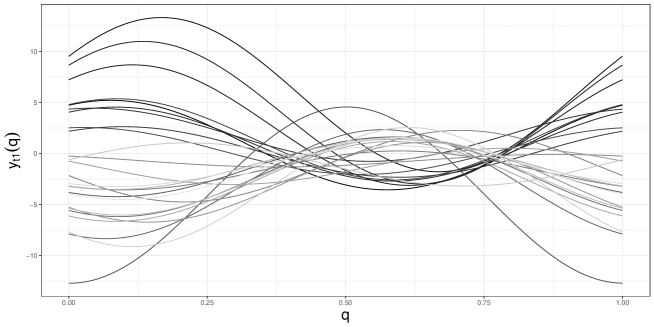
In so doing, the VAR(2) process is stable since $det(I_{3}-\bar{\Psi}_{1}\cdot u-\bar{\Psi}_{2}\cdot u^{2})\neq 0$ $\forall|u|\leq 1$. A graphical representation of a replication with $T=25$ is provided in Figure 1.

Figure 1: Graphical representation of the simulated data. The sample size is $T=25$, with older functions being darker.

Seven models are taken into account:

• Oracle Model The point predictions are obtained by considering both $\boldsymbol{g}(q)$ and $\bar{\Psi}_{1},\bar{\Psi}_{2}$ as known. In other words, the point prediction for $Y_{t1}(q)$ is simply given by $\boldsymbol{g}^{\prime}(q)(\bar{\Psi}_{1}\boldsymbol{\bar{y}}_{t-1}+\bar{\Psi}_{2}\boldsymbol{\bar{y}}_{t-2})$ $\forall t\in\{3,\dots,T+1\}$.

• VAR Models The point predictions are obtained by considering $\boldsymbol{g}(q)$ as known and $\bar{\Psi}_{1},\bar{\Psi}_{2}$ as unknown. Specifically, the point prediction for $Y_{t1}(q)$ is obtained by estimating $r$ matrices $\bar{\Psi}_{1},\dots,\bar{\Psi}_{r}$ by fitting a VAR(r) model on $\{\boldsymbol{\bar{z}}_{h}:h\in\mathcal{I}_{1}\}$, with $\boldsymbol{\bar{z}}_{h}=(\boldsymbol{\bar{x}}_{h},\boldsymbol{\bar{y}}_{h})$, $\boldsymbol{\bar{x}}_{h}=\{\boldsymbol{\bar{y}}_{h-1},\dots,\boldsymbol{\bar{y}}_{h-r}\}$ and $r\in\{1,2,3\}$. In so doing, the estimation issue is converted to a problem of estimating the Fourier coefficients [9].

• FAR Models The point predictions are obtained by considering both $\boldsymbol{g}(q)$ and $\bar{\Psi}_{1},\bar{\Psi}_{2}$ as unknown. The point predictions are obtained by fitting (on the training set, as usual) a concurrent function-on-function autoregressive model of order $r\in\{1,2,3\}$, i.e.:

  $$y_{t1}(q)=\sum_{i=1}^{r}\beta_{i}(q)y_{t-i,1}(q)+a_{t}(q),$$

  with $a_{t}(q)$ finite-variance mean-zero error process uncorrelated with the linear systematic component and such that $a_{t^{1}}$ is independent from $a_{t^{2}}$, $t^{1}\neq t^{2}$.

The purpose is to evaluate the procedure by taking into account scenarios characterized by a decreasing knowledge of the data generating process. The first model (Oracle Model) represents the ideal case in which the oracle nonconformity scores can be computed since both $\bar{\Psi}_{1},\bar{\Psi}_{2}$ and the subspace in which the observations lie are known, the second set of models (Var Models with $r\in\{1,2,3\}$) represents a more challenging case in which only the subspace in which the observations live is known, whereas the third set of models (FAR Models with $r\in\{1,2,3\}$) represents the general case in which the dynamic over time of the phenomenon must be derived by the available data. The simulation scheme here proposed allows to investigate, in addition to the Oracle Model and the case in which the model is correctly specified (VAR Model with $r=2$), three widespread kinds of model misspecification: the misspecification due to omitted relevant variable [VAR Model with $r=1$, see 27], misspecification due to inclusion of irrelevant variable [VAR Model with $r=3$, see 27] and the functional form misspecification [FAR Models, see 28, since the data generating process can not be rewritten as a FAR Model].

We consider $\mathcal{Q}_{1}=[0,1]$ and $\alpha=0.25$. In order to fulfill the four conditions required ($(l+1)/b$ integer-valued; $\alpha\in[b/(l+1),1)$; a training set size allowing to estimate a VAR(r) model; $\lfloor\alpha(l+1)/b\rfloor b/(l+1)=\alpha$ for consistency with the i.i.d. framework), we set $(T,l)=\{(25,7),(50,23),(100,47),(1000,479)\}$ when $b=1$, $(T,l)=\{(50,23),(100,47),(1000,479)\}$ when $b=3$ and $(T,l)=\{(100,47),(1000,479)\}$ when $b=6$. As usual in the time series setting, the first $r$ observations (2 observations when the Oracle Model is considered, respectively) are taken into account only as covariates, and so the training set size is equal to $T-l-r$ ($T-l-2$ when the Oracle Model is considered, respectively). Practically, for each value of $T$, we evaluate the procedure by considering $N=5000$ replications for each combination of point predictor and value of $b$. The simulations are achieved by using the R Programming Language [29], and the generation of data by fts.rar function of freqdom.fda package [30].

3.1 Results

Table 1 and Table 2

Table 1: Empirical coverage (99% confidence interval in brackets). Oracle Model. $\alpha$=0.25.

Empirical Coverage - Oracle Model
$\pagecolor{light-light-gray}b=1$	$\pagecolor{light-light-gray}T=25$	0.753[0.737,0.769]
	$\pagecolor{light-light-gray}T=50$	0.752[0.736,0.768]
	$\pagecolor{light-light-gray}T=100$	0.748[0.732,0.764]
	$\pagecolor{light-light-gray}T=1000$	0.743[0.727,0.759]
$\pagecolor{light-light-gray}b=3$	$\pagecolor{light-light-gray}T=50$	0.744[0.728,0.760]
	$\pagecolor{light-light-gray}T=100$	0.738[0.722,0.754]
	$\pagecolor{light-light-gray}T=1000$	0.743[0.727,0.759]
$\pagecolor{light-light-gray}b=6$	$\pagecolor{light-light-gray}T=100$	0.745[0.729,0.760]
	$\pagecolor{light-light-gray}T=1000$	0.743[0.727,0.759]

Table 2: Empirical coverage (99% confidence interval in brackets). VAR Models and FAR Models. $\alpha$=0.25. The values in bold indicate that the corresponding conf. intervals do not include $1-\alpha$.

Empirical Coverage - VAR Model
		r=1	r=2	r=3
$\pagecolor{light-light-gray}b=1$	$\pagecolor{light-light-gray}T=25$	0.741[0.725,0.757]	0.735[0.719,0.751]	0.754[0.738,0.770]
	$\pagecolor{light-light-gray}T=50$	0.737[0.721,0.753]	0.746[0.730,0.762]	0.742[0.726,0.758]
	$\pagecolor{light-light-gray}T=100$	0.731[0.714,0.747]	0.743[0.727,0.759]	0.738[0.722,0.754]
	$\pagecolor{light-light-gray}T=1000$	0.743[0.727,0.759]	0.744[0.728,0.760]	0.742[0.726,0.758]
$\pagecolor{light-light-gray}b=3$	$\pagecolor{light-light-gray}T=50$	0.735[0.719,0.751]	0.742[0.726,0.758]	0.743[0.727,0.759]
	$\pagecolor{light-light-gray}T=100$	0.737[0.721,0.753]	0.738[0.722,0.754]	0.736[0.720,0.752]
	$\pagecolor{light-light-gray}T=1000$	0.743[0.727,0.759]	0.745[0.729,0.761]	0.744[0.728,0.760]
$\pagecolor{light-light-gray}b=6$	$\pagecolor{light-light-gray}T=100$	0.737[0.721,0.753]	0.740[0.724,0.756]	0.741[0.725,0.757]
	$\pagecolor{light-light-gray}T=1000$	0.746[0.730,0.762]	0.745[0.729,0.761]	0.743[0.727,0.759]
Empirical Coverage - FAR Model
		r=1	r=2	r=3
$\pagecolor{light-light-gray}b=1$	$\pagecolor{light-light-gray}T=25$	0.745[0.729,0.761]	0.742[0.726,0.758]	0.741[0.725,0.757]
	$\pagecolor{light-light-gray}T=50$	0.738[0.722,0.754]	0.750[0.734,0.766]	0.747[0.731,0.763]
	$\pagecolor{light-light-gray}T=100$	0.733[0.717,0.749]	0.742[0.726,0.758]	0.740[0.724,0.756]
	$\pagecolor{light-light-gray}T=1000$	0.743[0.727,0.759]	0.742[0.726,0.758]	0.743[0.727,0.759]
$\pagecolor{light-light-gray}b=3$	$\pagecolor{light-light-gray}T=50$	0.736[0.720,0.752]	0.750[0.734,0.766]	0.742[0.726,0.758]
	$\pagecolor{light-light-gray}T=100$	0.736[0.720,0.752]	0.738[0.722,0.754]	0.743[0.727,0.759]
	$\pagecolor{light-light-gray}T=1000$	0.741[0.725,0.757]	0.744[0.728,0.760]	0.743[0.727,0.759]
$\pagecolor{light-light-gray}b=6$	$\pagecolor{light-light-gray}T=100$	0.736[0.720,0.752]	0.742[0.726,0.758]	0.740[0.724,0.756]
	$\pagecolor{light-light-gray}T=1000$	0.745[0.729,0.760]	0.744[0.728,0.760]	0.744[0.728,0.760]

show the empirical coverage, together with the related 99% confidence interval in square brackets, reached by the procedure presented in the manuscript. Specifically, the empirical coverage is simply computed as the fraction of the $N=5000$ replications in which $\boldsymbol{y}_{T+1}$ belongs to $\mathcal{C}_{T,1-\alpha}\left(\boldsymbol{x}_{T+1}\right)$, and the confidence interval is reported in order to provide an idea of the variability of the phenomenon, rather than to make inferential conclusion on the unconditional coverage in the various settings. The evidence is quite satisfactory as for any value of $b$, sample size $T$ and model the empirical coverage is close to $1-\alpha=0.75$, as suggested by the fact that only 2 out of the 63 confidence intervals (the cells in bold in the tables) do not include the nominal confidence level. The result provided by the simulation study is particularly appealing since it suggests that an appropriate coverage is reached also when the sample size is very small, a fact that allows the procedure to be applied in many practical frameworks.

Although comparing the size of prediction bands obtained in scenarios characterized by (potentially) different unconditional coverages may lead to misleading conclusions, in light of the evidence provided so far we evaluate this aspect when the model, the value of $T$ and the value of $b$ vary. To do that, we define, according to the definition given in [19], the size of a multivariate prediction band as the sum of the $p$ areas between the upper and lower bound of the $p$ univariate prediction bands, i.e. $\sum_{j=1}^{p}\int_{\mathcal{Q}_{j}}2\cdot k^{s}\cdot s_{j,\mathcal{I}_{1}}(q)dq$ (that, in this case, is simply $\int_{\mathcal{Q}_{1}}2\cdot k^{s}\cdot s_{1,\mathcal{I}_{1}}(q)dq$). Figure 2, 3, 4, 5, 6, 7, 8

Figure 2: Set size. Oracle Model. $\alpha=0.25$.

Figure 3: Set size. VAR Model, $r=1$. $\alpha=0.25$.

Figure 4: Set size. VAR Model, $r=2$. $\alpha=0.25$.

Figure 5: Set size. VAR Model, $r=3$. $\alpha=0.25$. For visualization purpose, the most extreme value (equal to 210.54) obtained when $b=1$, $T=25$ is removed.

Figure 6: Set size. FAR Model, $r=1$. $\alpha=0.25$.

Figure 7: Set size. FAR Model, $r=2$. $\alpha=0.25$.

Figure 8: Set size. FAR Model, $r=3$. $\alpha=0.25$.

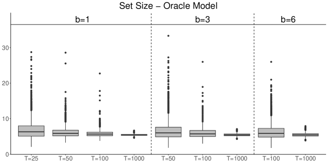
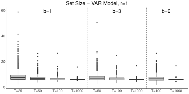
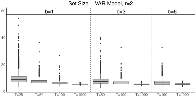
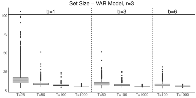
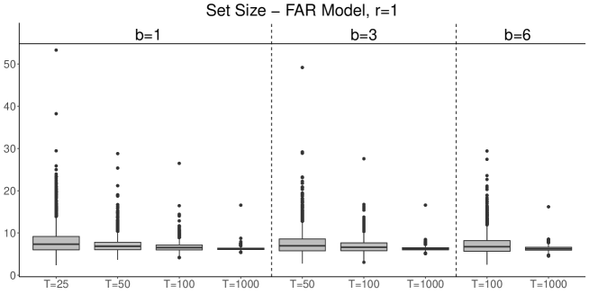
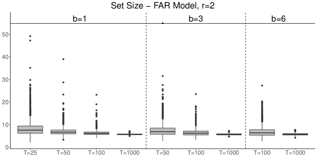
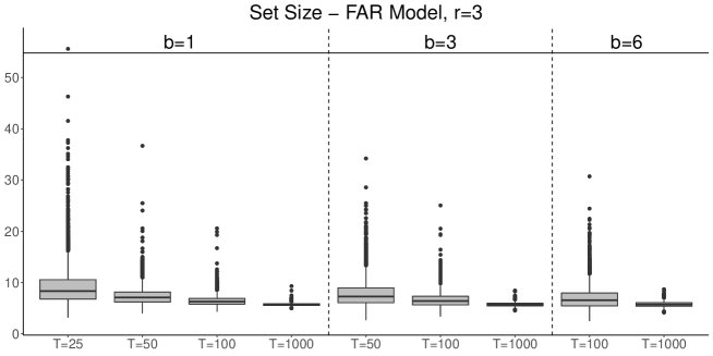
show the boxplots concerning the size of the $N=5000$ prediction bands. By considering each point predictor separately, it is possible to notice that, given $b$, the band size tends to decrease when $T$ increases and, given $T$, it tends to decrease when $b$ decreases: this evidence is not surprising since when $T$ increases (and so $l$) and when $b$ decreases a greater number of nonconformity scores is computed. Also the training set size has a relevant impact on the phenomenon since one is justified in expecting the band size to decrease when $m$ grows because more accurate regression estimates provide smaller nonconformity scores, as suggested by analyzing the three couples $(T,b)=\{(25,1),(50,3),(100,6)\}$ in which the number of nonconformity scores computed is constant.

The Oracle model outperforms the VAR models and the FAR models for every value of $T$, $b$, as expected. By considering the VAR models and the FAR models, when the sample size is very small ($T$=25) the order of the model providing the best performance in terms of size is $r=1$ since higher values of $r$ may provide unstable estimation procedures. Vice versa, the importance of using a model correctly specified is evident when $T$ is large: indeed, the VAR Model with $r=2$ represents the best choice overall (Oracle Model excluded) when $T=1000$, and it outperforms the other two VAR models ($r=1$, $r=3$) also when $T=100$. Specifically, when $T=1000$ the VAR model with a relevant variable omitted ($r=1$) is largely outperformed by the other two VAR models ($r=1$, $r=3$) since the estimation of a single matrix $\bar{\Psi}_{1}$ represents an undeniable limit in obtaining accurate regression estimates.

In light of the evidence provided in this Section, the procedure seems reliable in the frequent practical scenarios characterized by small sample size and/or model misspecification, whereas $b=1$ represents the best balance between guarantee in terms of coverage and exhaustive use of the information provided by the available data.

4 Application to the Italian Gas Market

In this Section, we apply the procedure developed in Section 2 to a specific Italian gas market, namely the MGS (Mercato Gas in Stoccaggio), in order to create simultaneous prediction bands for the daily offer and demand curves. It should nevertheless be noted that our method can be applied to many application scenarios, such as other energy or non-energy markets. The MGS is a market in which users - authorized by the energy regulator Gestore Mercati Energetici (GME) - and the pipeline manager (Snam S.p.A.) day by day submit supply offers and demand bids for the gas stored, which is traded through an auction mechanism.

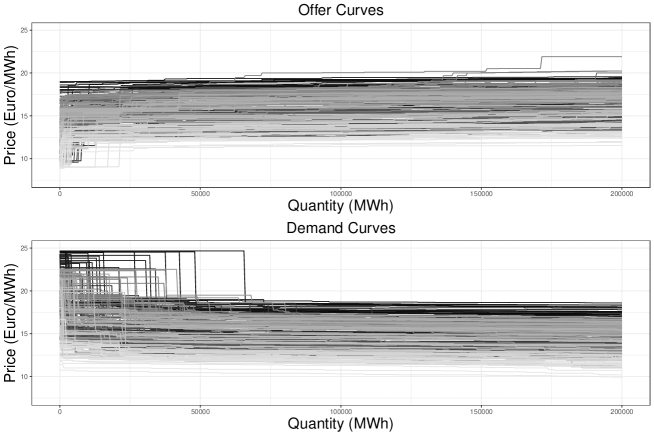
Specifically, for each day the supply offers (demand bids, respectively) are sorted by price in ascending (descending, respectively) order, and the demand and offer curves are built - starting from raw data provided in XML format by GME (https://www.mercatoelettrico.org/en/) - by considering the cumulative sum of the quantities (expressed in MWh). In doing so, by construction both daily offer and demand curves are positive monotonic (increasing and decreasing, respectively) step functions. The intersection of the two curves provides the price $P_{t}$ at which the gas is traded (expressed in Euro/MWh) and the total quantity exchanged $Q_{t}$, and every offer/bid to the left of the intersection is accepted and consequently traded at price $P_{t}$.

The creation of prediction bands is strategic for energy traders’ decision-making since it allows to evaluate the possible effect of offers/bids on the shape of the curves (and consequently on both the price $P_{t}$ and the quantity exchanged $Q_{t}$), an aspect that cannot be directly included by usual non-functional procedures for interval price prediction. In order to show the useful insights that the procedure built in Section 2 can provide, we create simultaneous prediction bands for the offer ($Y_{t1}$) and demand ($Y_{t2}$) curve for each day in the six-month period between 1 August 2019 and 31 January 2020. For each of the 184 days we aim to predict, we build the corresponding prediction band based on the information provided by the rolling window of $90$ days (i.e. $T=90$) including the most up-to-date information available. We set the function domains $\mathcal{Q}_{1}=\mathcal{Q}_{2}=[0,2\cdot 10^{5}]$ as all demand and offer curves are observed in this range and at the same time the total quantity exchanged $Q_{t}$ always belongs to this interval in the period taken into account. The offer and demand curves considered in the analysis are displayed in Figure 9.

Figure 9: The offer (at the top) and demand (at the bottom) curves considered in the analysis, with older functions being darker.

In order to obtain the needed point predictions, we consider the following simple concurrent function-on-function autoregressive model with a scalar covariate:

$$y_{tj}(q)=\beta_{1j}(q)y_{t-8,j}(q)+\beta_{2j}(q)P_{t-2}+a_{t}(q),\quad j\in\{1,2\},\quad q\in\mathcal{Q}_{j},$$ (4)

with $a_{t}(q)$ defined as in Section 3. The inclusion of the lagged curve at time $t-8$ and of the lagged (scalar) price at time $t-2$ is motivated by the fact that they represent the most up-to-date information available for a trader participating in the auction for day $t$ due to GME’s regulation. However, model (4) does not guarantee that the point predictions are monotonic functions. In view of this, after obtaining $\hat{\beta}_{1j},\hat{\beta}_{2j}$ $\forall j=1,2$, we simply obtain monotonic point predictions by defining the point prediction for the offer curve at time $t$ evaluated at $q$, i.e. $[\hat{\mu}^{1}_{\mathcal{I}_{1}}(x_{t,1})](q)$, as follows:

$$[\hat{\mu}^{1}_{\mathcal{I}_{1}}(x_{t,1})](q)=\begin{cases}\hat{y}_{t,1}(q)&\text{if $\hat{y}_{t,1}(q)=\max_{x\in[0,q]}\hat{y}_{t,1}(x)$}\\ \hat{y}_{t,1}(q^{{}^{\prime}})+(q-q^{{}^{\prime}})\left(\frac{\hat{y}_{t,1}(q^{{}^{\prime\prime}})-\hat{y}_{t,1}(q^{{}^{\prime}})}{q^{{}^{\prime\prime}}-q^{{}^{\prime}}}\right)&\text{otherwise}\\ \end{cases}$$ (5)

with $\hat{y}_{t,1}$ the predicted offer curve obtained by fitting model (4) using OLS, $q^{{}^{\prime}}:=\max\left\{\mathrm{argmax}_{x\in[0,q]}\hat{y}_{t,1}(x)\right\}$ and $q^{{}^{\prime\prime}}:=\min\left\{x\in[q,200000]|\hat{y}_{t,1}(x)\geq\hat{y}_{t,1}(q)\right\}$. The specular procedure is developed to obtain $[\hat{\mu}^{2}_{\mathcal{I}_{1}}(x_{t,2})](q)$, i.e. the point prediction for the demand curve at time $t$ evaluated at $q$. Vice versa, the fact that the point predictions are not step functions does not represent a limit since the prices at which the steps happen can be absolutely continuous random variables, and consequently the expectation of this kind of random step function is a continuous function [31]. Model (4) and the correction induced by (5) certainly represent an oversimplification of the phenomenon analyzed, and one is justified in expecting other variables (such as the trading activity on the other energy markets) to have an important impact on the MGS’s dynamics: however, the purpose of this Section is to illustrate the application potential of the procedure presented in Section 2 in a general and arbitrary prediction scenario, rather than when a particularly sophisticated model is built.

The last, fundamental step is the definition of the significance level $\alpha$, of the calibration set size $l$, of the training set size $m$ and of $b$. We consider two possible values of $\alpha$, i.e. 0.5 and 0.25, and $b=1$ in light of the evidence provided by Section 3. We also set $l=39$ and, given the aforementioned delay in the information concerning lagged curves, we consider $m=T-l-8=43$ in order to obtain a value of $m/l$ close to 1 and a value of $l$ such that $\lfloor\alpha(l+1)/b\rfloor b/(l+1)=\alpha$, as in Section 3.

Figure 10

Figure 10: Multivariate prediction bands with $\alpha=0.5$ (darker regions) and $\alpha=0.25$ (lighter regions). The continuous lines represent the observed offer and demand curves, whereas the dashed lines represent the fitted ones. The black cross indicates $(Q_{t},P_{t})$.

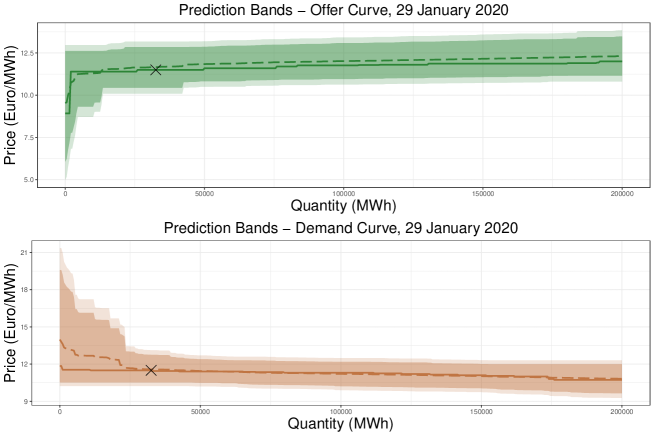
shows the multivariate prediction bands obtained for one of the day we aim to predict (29 January 2020), with the panel at the top (at the bottom, respectively) showing the portions of the multivariate prediction bands related to the offer curve (demand curve, respectively): in both cases, the darker region indicates the prediction bands obtained by considering $\alpha=0.5$ (i.e. nominal confidence level $1-\alpha=0.50$), whereas the lighter one denotes those obtained by considering $\alpha=0.25$ (i.e. nominal confidence level $1-\alpha=0.75$). For the sake of completeness, the observed (continuous line) and fitted (dashed line) curves, together with the price $P_{t}$ and the quantity exchanged $Q_{t}$ (black cross), are also displayed. Since the curves are monotonic by construction, the upper and the lower bounds of the prediction bands were made monotonic before being plotted: indeed, the procedure does not guarantee that such bounds are monotonic, but the fully nonparametric approach induced by the permutation scheme $\Pi$ allows to made them monotonic by removing portions of the prediction bands associated to regions of the functional space that violate known features (e.g. monotonicity) of the function to be predicted, without decreasing the unconditional coverage. It is absolutely evident that the prediction bands are decidedly wider in the first part of the domain, especially in the panel at the bottom of the figure, and this is due to the fact that the behavior of the two curves in that portion of the domain is hardly predictable. The main reason of this phenomenon is the conduct of the pipeline manager Snam S.p.A.: indeed, in the period considered it typically submits extremely low supply offers and high demand bids - if compared to other traders’ offers/bids - in order to be sure to sell/buy the quantity needed, but this makes the uncertainty quantification a particularly tough task if no information on Snam’s trading intentions is available. As proof of that, we created a fictional scenario by removing all the offers/bids made by Snam in the period considered, and we therefore computed the corresponding 184 multivariate prediction bands in the period 1 August 2019-31 January 2020: in doing so, the size in the initial part of the domain [0,25000] of the two univariate prediction bands composing each multivariate prediction band (related to the offer and demand curve respectively, and formally defined as $\int_{0}^{25000}2\cdot k^{s}\cdot s_{j,\mathcal{I}_{1}}(q)dq$, $j=1,2$) decreases by 45.2% (median value) for the offer curve and by 72.4% (median value) for the demand curve when $\alpha=0.50$ is considered. A very similar result is obtained when $\alpha=0.25$ is taken into account. In view of this, the inclusion in model (4) of information aimed at capturing Snam’s behavior represents a possible future development that is highly likely to create smaller (and consequently more informative) prediction bands.

A further useful by-product of the procedure related to this specific application is that it allows to automatically obtain a prediction region for $(Q_{t},P_{t})$ by considering the region in which the prediction band for the offer curve and that for the demand curve overlap. As an example, the region for 29 January 2020 computed with $\alpha=0.50$ is represented in the left panel of Figure 11.

Figure 11: The left panel shows the prediction region for $(Q_{t},P_{t})$ (29 January 2020, $\alpha=0.50$), together with the value of $(Q_{t},P_{t})$ effectively observed (black cross). The right panel shows the same prediction region (dashed darker lines) and the prediction region obtained by submitting an extra demand bid of 20000 MWh at 12 Euro/MWh (lighter region).

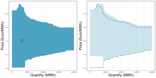
By computing the fraction of times that the observed $(Q_{t},P_{t})$ effectively belongs to the prediction region thus obtained over the 184 days considered, we obtain that 92.4% of the time the observed prediction region contains the observed intersection point when $\alpha=0.50$, and that 97.8% of the time when $\alpha=0.25$. This evidence is appealing especially when compared to the fraction of times that the observed offer and demand curves effectively belong to the observed multivariate prediction bands, that is 52.7% when $\alpha=0.50$ (i.e. nominal confidence level $1-\alpha=0.50$) and 75.5% when $\alpha=0.25$ (i.e. nominal confidence level $1-\alpha=0.75$), respectively. It is fundamental to notice that the last two percentages do not represent empirical coverages, and more generally provide no relevant information about the unconditional coverage reached by the procedure developed, since the prediction bands computed in this Section are obtained by repeating the procedure day after day and by considering a rolling window. However, it is still possible to obtain a theoretical result concerning the unconditional coverage of the aforementioned prediction region by simply reasoning about how it is built: indeed, by construction if the observed offer curve and the observed demand curve effectively jointly belong to the observed multivariate prediction band, and if the intersection point exists (an event always verified in the period considered), then the intersection point necessarily belongs to the area in which the two univariate prediction bands overlap. As a consequence, by construction, if the two curves intersect, than the unconditional coverage reached by the prediction region is greater or equal than $\mathbb{P}\left(\boldsymbol{Y}_{T+1}\in\mathcal{C}_{T,1-\alpha}\left(\boldsymbol{X}_{T+1}\right)\right)$. In light of this and of the empirical results provided, we conclude that the prediction region naturally induced by the method described in Section 2 represents a promising tool - both from a theoretical and an application point of view - that can be profitably included in traders’ tool kit.

The analysis here presented also allows to exploit the market from a speculative perspective: indeed, from a given trader’s point of view, the procedure presented in this manuscript allows to directly evaluate the impact of any extra offer/bid on the prediction bands for tomorrow’s offer and demand curves, and consequently on the prediction region for the intersection point. As an example, a trader may want to evaluate the effect of a demand bid of 20000 MWh at 12 Euro/MWh on tomorrow’s intersection point: to do that, the user can add this bid to the predicted demand curve, thereby inducing a change in the multivariate prediction band and consequently in the prediction region. The resulting prediction region for 29 January 2020 is displayed in the right panel of Figure 11.

The evidence showed in this Section is obviously limited to a few examples. In order to provide a comprehensive overview of the results obtained in the period considered, we developed a Shiny app (available at https://jacopodiquigiovanni.shinyapps.io/ItalianGasMarketApp/) that allows to interactively choose the scenario of interest and to visualize the associated results. Specifically, the top left panel allows the user to dynamically change five inputs, that are: the day for which the predictions are made (between 1 August 2019 and 31 January 2020), the nominal confidence level $1-\alpha$, the type of extra bid/offer (assuming two possible values: Demand, Offer) you want to evaluate the impact of, its quantity and its price. The top right panel and the bottom right panel show the portion of multivariate prediction band related to the offer and demand curve respectively, together with the observed curves, for the day and the nominal confidence level selected. In doing so, it is possible to verify whether the couple of curves would have been contained in the multivariate prediction band or not if the procedure had been implemented in the real world. Finally, the bottom left panel shows the prediction region for $(Q_{t},P_{t})$ obtained for the day and the nominal confidence level selected (dark blue region), as well as the value of $(Q_{t},P_{t})$ effectively observed (red cross), allowing the user to check the accuracy of the prediction. In addition, it shows also the prediction region obtained by including the extra bid/offer in tomorrow’s predicted demand/offer curve (light blue region), allowing this tool to be used for the purposes mentioned above.

5 Conclusions and Further Developments

The present work deals with the issue of forecasting demand and supply curves in on the Gas Market, proposing methods able to quantify uncertainty in the multivariate functional time series prediction framework, a new and particularly relevant workhorse in the energy trading field. The approach developed in this article extends the non-overlapping blocking scheme proposed by Chernozhukov et al. [20] to the Split context in order to create simultaneous prediction bands for forthcoming multivariate random function $\boldsymbol{Y}_{T+1}$. The procedure inherits the guarantees for the unconditional coverage in terms of finite-sample performance bounds and of asymptotic exactness under some conditions concerning the oracle nonconformity measure $A^{*}$ and the nonconformity measure $A$, but can be also satisfactorily applied to the multivariate functional context due to the Split process and to the specific nonconformity measure used [firstly introduced by 19]. Theorem 2.1 provides a theoretically sound prediction framework based on assumptions similar to the ones introduced by Chernozhukov et al. [20]. However these assumptions could be tricky to assess in practice. For this reason, we combined our theoretical work with a simulation study aimed at evaluating the procedure in situations in which Theorem 2.1 is violated, as in the case of model misspecification. The results obtained are encouraging: the empirical coverage values are close to the nominal confidence level $1-\alpha$ also when the sample size $T$ is small or the model is misspecified, regardless the value of $b$. In view of this, we applied the method described in Section 2 to a real-world scenario of strong interest, namely the prediction of daily offer and demand curves in the Italian gas market. We built the corresponding simultaneous prediction bands for each day in a six-month period based on a rolling window including the most up-to-date information available. Despite the fact that the point predictors considered can surely be improved to provide more accurate regression estimates, we used standard functional regression estimators to show the wide applicability of the procedure, also in a speculative perspective. In order to provide a complete overview of the study, we developed a Shiny app able to display the predicted bands, as well as the related prediction regions for $(Q_{t},P_{t})$, under several operative conditions. Being based on a Split framework, our proposal shares both the strenghts (namely, the simple mathematical tractability and ease of implementation) and the weaknesses of the prediction methods based on Split Conformal. In fact the random subdivision of the sample intrinsically induces an element of randomness in the method and is not particularly efficient in its use of data. To improve on this, a very promising area of research is to employ derivations of the original Conformal approach such as the jackknife+ procedure [32] and extensions [see, for example, 33] in a functional context.

T

he authors are grateful to Centrex Italia S.p.A. which provided a detailed overview of the Italian gas market. M.F. and S.V. acknowledge the financial support of Accordo Quadro ASI-POLIMI “Attività di Ricerca e Innovazione” n. 2018-5-HH.0, collaboration agreement between the Italian Space Agency and Politecnico di Milano.

References

- Canale and Vantini [2016] A. Canale, S. Vantini, Constrained functional time series: Applications to the Italian gas market, Int. J. Forecast. 32 (2016) 1340–1351.
- Shah and Lisi [2020] I. Shah, F. Lisi, Forecasting of electricity price through a functional prediction of sale and purchase curves, J. Forecast. 39 (2020) 242–259.
- Ramsay and Silverman [2005] J. O. Ramsay, B. W. Silverman, Functional data analysis, Springer series in statistics, Springer, 2005.
- Ferraty and Vieu [2006] F. Ferraty, P. Vieu, Nonparametric Functional Data Analysis: Theory and Practice, Springer Series in Statistics, Springer-Verlag, New York, 2006.
- Horváth and Kokoszka [2012] L. Horváth, P. Kokoszka, Inference for Functional Data with Applications, Springer Series in Statistics, Springer-Verlag, New York, 2012.
- Wang et al. [2016] J.-L. Wang, J.-M. Chiou, H.-G. Müller, Functional Data Analysis, Annu. Rev. Stat. Appl. 3 (2016) 257–295.
- Rossini and Canale [2019] J. Rossini, A. Canale, Quantifying prediction uncertainty for functional-and-scalar to functional autoregressive models under shape constraints, J. Multivariate Anal. 170 (2019) 221–231.
- Hörmann and Kokoszka [2012] S. Hörmann, P. Kokoszka, Functional Time Series, in: Handbook of Statistics, volume 30 of Time Series Analysis: Methods and Applications, Elsevier, 2012, pp. 157–186.
- Chen et al. [2021] Y. Chen, T. Koch, K. G. Lim, X. Xu, N. Zakiyeva, A review study of functional autoregressive models with application to energy forecasting, Wiley Interdiscip. Rev. Comput. Stat. 13 (2021) e1525.
- Ferraty et al. [2002] F. Ferraty, A. Goia, P. Vieu, Functional nonparametric model for time series: a fractal approach for dimension reduction, Test 11 (2002) 317–344.
- Ferraty and Vieu [2004] F. Ferraty, P. Vieu, Nonparametric models for functional data, with application in regression, time series prediction and curve discrimination, J. Nonparametr. Stat. 16 (2004) 111–125.
- Hyndman and Shang [2009] R. J. Hyndman, H. L. Shang, Forecasting functional time series, J. Korean Statist. Soc. 38 (2009) 199–211.
- Gao and Shang [2017] Y. Gao, H. L. Shang, Multivariate Functional Time Series Forecasting: Application to Age-Specific Mortality Rates, Risks 5 (2017) 21.
- Paparoditis and Shang [2021] E. Paparoditis, H. L. Shang, Bootstrap Prediction Bands for Functional Time Series, arXiv:2004.03971 (2021).
- Vovk et al. [2005] V. Vovk, A. Gammerman, G. Shafer, Algorithmic learning in a random world, Springer Science & Business Media, 2005.
- Gammerman et al. [1998] A. Gammerman, V. Vovk, V. Vapnik, Learning by Transduction, in: Proceedings of the Fourteenth Conference on Uncertainty in Artificial Intelligence, UAI’98, Morgan Kaufmann Publishers Inc., San Francisco, CA, USA, 1998, pp. 148–155.
- Zeni et al. [2020] G. Zeni, M. Fontana, S. Vantini, Conformal prediction: a unified review of theory and new challenges, arXiv:2005.07972 (2020).
- Diquigiovanni et al. [2021] J. Diquigiovanni, M. Fontana, S. Vantini, The importance of being a band: Finite-sample exact distribution-free prediction sets for functional data, arXiv:2102.06746 (2021).
- Diquigiovanni et al. [2022] J. Diquigiovanni, M. Fontana, S. Vantini, Conformal prediction bands for multivariate functional data, Journal of Multivariate Analysis 189 (2022) 104879.
- Chernozhukov et al. [2018] V. Chernozhukov, K. Wüthrich, Y. Zhu, Exact and robust conformal inference methods for predictive machine learning with dependent data, in: Conference On Learning Theory, Proceedings of Machine Learning Research, 2018, pp. 732–749.
- Inselberg [1985] A. Inselberg, The plane with parallel coordinates, Vis Comput 1 (1985) 69–91.
- Rubin [1984] D. B. Rubin, Bayesianly justifiable and relevant frequency calculations for the applies statistician, Ann. Statist 12 (1984) 1151–1172.
- Romano [1990] J. P. Romano, On the behavior of randomization tests without a group invariance assumption, J. Amer. Statist. Assoc. 85 (1990) 686–692.
- Lehmann and Romano [2006] E. L. Lehmann, J. P. Romano, Testing statistical hypotheses, Springer Science & Business Media, 2006.
- Shafer and Vovk [2008] G. Shafer, V. Vovk, A Tutorial on Conformal Prediction, J. Mach. Learn. Res. 9 (2008) 371–421.
- Lei et al. [2013] J. Lei, J. Robins, L. Wasserman, Distribution-free prediction sets, J. Amer. Statist. Assoc. 108 (2013) 278–287.
- Rao [1971] P. Rao, Some notes on misspecification in multiple regressions, Amer. Statist. 25 (1971) 37–39.
- Wooldridge [1994] J. M. Wooldridge, A simple specification test for the predictive ability of transformation models, Rev. Econ. Stat. 76 (1994) 59–65.
- R Core Team [2018] R Core Team, R: A Language and Environment for Statistical Computing, R Foundation for Statistical Computing, Vienna, Austria, 2018. URL: https://www.R-project.org/.
- Hormann and Kidzinski [2017] Hormann and Kidzinski, freqdom.fda: Functional Time Series: Dynamic Functional Principal Components, 2017. URL: https://CRAN.R-project.org/package=freqdom.fda.
- Pelagatti [2013] M. Pelagatti, Supply function prediction in electricity auctions, in: Complex Models and Computational Methods in Statistics, Springer, 2013, pp. 203–213.
- Barber et al. [2021] R. F. Barber, E. J. Candes, A. Ramdas, R. J. Tibshirani, Predictive inference with the jackknife+, Ann. Statist. 49 (2021) 486–507.
- Xu and Xie [2020] C. Xu, Y. Xie, Conformal prediction interval for dynamic time-series, arXiv:2010.09107 (2020).