11institutetext: Instituto Superior Técnico, University of Lisbon, Portugal
22institutetext: INESC-ID, Lisbon, Portugal

Limited depth bandit-based strategy for Monte Carlo planning in continuous action spaces

Ricardo Quinteiro 11    Francisco S. Melo 1122    Pedro A. Santos 1122
Abstract

This paper addresses the problem of optimal control using search trees. We start by considering multi-armed bandit problems with continuous action spaces and propose LD-HOO, a limited depth variant of the hierarchical optimistic optimization (HOO) algorithm. We provide a regret analysis for LD-HOO and show that, asymptotically, our algorithm exhibits the same cumulative regret as the original HOO while being faster and more memory efficient. We then propose a Monte Carlo tree search algorithm based on LD-HOO for optimal control problems and illustrate the resulting approach’s application in several optimal control problems.

Abstract

This appendix includes a detailed proof for Theorem 3.1, establishing an asymptotic regret bound for LD-HOO.

Keywords:
Multiarmed bandits Monte Carlo tree search Planning in continuous action space

1 Introduction

Recent years have witnessed remarkable successes of artificial intelligence, brought about by the effective combination of powerful machine learning algorithms based on neural networks and efficient planning approaches based on Monte Carlo tree search. Perhaps the most celebrated is AlphaGo and its successors [15, 17, 16, 14], which could attain super-human proficiency in several complex games such as chess, Go, or Shogi. Even before AlphaGo, Monte Carlo tree search approaches were already widely used in complex planning problems due to their efficiency, mild requirements, and robust theoretical guarantees [3] .

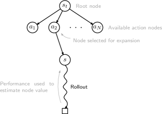
Monte Carlo tree search (MCTS) is a family of online planning methods initially designed to solve sequential decision problems such as Markov decision problems [7, 6]. At each step t𝑡t, the decision-maker builds a search tree with its current state, stsubscript𝑠𝑡s_{t}, as the root node. Its children correspond to the actions available to the agent at stsubscript𝑠𝑡s_{t}, and the algorithm proceeds by estimating a value for each such action by using rollouts and efficient exploration. Rollouts provide empirical estimates for the nodes’ values in the tree, while efficient exploration directs tree expansion towards the more promising regions of the state space (see Fig. 1 for an illustration).
Refer to caption
Figure 1: Illustration of MCTS. An adequate exploration policy is used to determine the next node selected for expansion. Rollouts (i.e., sampled trajectories) from the expanded nodes are used to build estimates about how good the nodes are.

In this paper, we extend the idea behind MCTS to control problems with a continuous action space. The main challenge lies in ensuring efficient exploration. Standard MCTS approaches assume that the decision-maker has only a finite set of possible actions available and typically use multi-armed bandit algorithms to guide exploration. Hence, our first contribution is a novel multi-armed bandit algorithm for continuous action spaces.

Several works have addressed multi-armed bandits with continuous action spaces [11]. Most such approaches consider an action space that corresponds to a hypercube in Psuperscript𝑃\mathds{R}^{P}, i.e., a set

𝒳=p=1P[ap,bp],for ap,bpP.𝒳superscriptsubscriptproduct𝑝1𝑃subscript𝑎𝑝subscript𝑏𝑝for ap,bpP.\mathcal{X}=\prod_{p=1}^{P}[a_{p},b_{p}],\qquad\text{for $a_{p},b_{p}\in\mathds{R}^{P}$.}

Multi-armed bandit problems in continuous action settings generally apply some form of hierarchical partitioning [11]. Hierarchical partitioning successively splits 𝒳𝒳\mathcal{X} into smaller hypercubes in such a way that the resulting partition can be represented as a tree (see Fig. 2). Examples of such algorithms include deterministic optimistic optimization (DOO) [10], hierarchical optimistic optimization (HOO) [5], stochastic simultaneous optimistic optimization (StoSOO) [11], truncated hierarchical optimistic optimization (T-HOO) [4], or polynomial hierarchical optimistic optimization (Poly-HOO) [9].

Refer to caption
Figure 2: Hierarchical partitioning. The set 𝒳𝒳\mathcal{X} is successively split in uniform subsets, and the resulting partition can be represented as a K𝐾K-ary tree. The sets in level hh are referred as “cells” and denoted as 𝒳h,isubscript𝒳𝑖\mathcal{X}_{h,i}, with 0iKh10𝑖superscript𝐾10\leq i\leq K^{h}-1. Each set 𝒳h,isubscript𝒳𝑖\mathcal{X}_{h,i} is represented by a specific element xh,isubscript𝑥𝑖x_{h,i}, referred as the center of 𝒳h,isubscript𝒳𝑖\mathcal{X}_{h,i}.

All the methods above also build on the principle of optimism in the face of uncertainty, widely used in the multi-armed bandit literature [1] and MCTS. The most adequate for the settings considered in this paper are HOO and its truncated and polynomial variants. Unlike DOO, HOO admits stochastic rewards. Unlike StoSOO, it is an anytime algorithm, a desirable property when used within MCTS. Unfortunately, HOO exhibits quadratic runtime, which is inconvenient for MCTS. Poly-HOO and T-HOO are faster, but exhibit a worse performance in terms of cumulative regret.

This paper contributes LD-HOO, a modified version of HOO that is computationally faster but retains HOO’s guarantees in terms of cumulative regret. We also contribute an analysis of LD-HOO in terms of cumulative regret. Finally, we propose LD-HOOT (LD-HOO for trees), a novel MCTS algorithm for problems with continuous action spaces that uses LD-HOO for efficient exploration. We illustrate the application of LD-HOOT in several well-known optimal control problems.

2 Background

This section provides an overview of key concepts regarding the decision problems addressed in this paper and sets the notation used throughout.

2.1 The (stochastic) multi-armed bandit problem

We consider the problem of a decision maker that must, at each time step t=1,2,𝑡12t=1,2,\ldots, select a (possibly random) action Xtsubscript𝑋𝑡X_{t} from a set 𝒳𝒳\mathcal{X} of possible actions. Upon selecting an action Xt=xsubscript𝑋𝑡𝑥X_{t}=x, the decision maker receives a (possibly random) reward Ytsubscript𝑌𝑡Y_{t} with mean value f(x)𝑓𝑥f(x). The process then repeats.

We assume that Yt[0,1]subscript𝑌𝑡01Y_{t}\in[0,1] and the distribution governing Ytsubscript𝑌𝑡Y_{t} is stationary and independent of the past given the action Xtsubscript𝑋𝑡X_{t}. The function f:𝒳:𝑓𝒳f:\mathcal{X}\to\mathds{R} is unknown to the decision maker. The goal of the decision maker is to select the actions Xt,t=1,2,formulae-sequencesubscript𝑋𝑡𝑡12X_{t},t=1,2,\ldots, to maximize the total reward received.

A policy is a sequence π={πt,t=1,2,}\pi=\left\{\pi_{t},\;t=1,2,\ldots\right\}, where each πtsubscript𝜋𝑡\pi_{t} maps the history of the agent up to time step t𝑡t to a distribution over 𝒳𝒳\mathcal{X}. The cumulative regret of a policy π𝜋\pi at time step n𝑛n is defined as

R^n=nf(x)t=1nYt,subscript^𝑅𝑛𝑛𝑓superscript𝑥superscriptsubscript𝑡1𝑛subscript𝑌𝑡\hat{R}_{n}=nf(x^{*})-\sum_{t=1}^{n}Y_{t},

where x=argmaxx𝒳f(x)superscript𝑥subscriptargmax𝑥𝒳𝑓𝑥x^{*}=\operatorname*{\mathrm{argmax}}_{x\in\mathcal{X}}f(x), and the cumulative pseudo-regret is

Rn=nf(x)t=1nf(xt).subscript𝑅𝑛𝑛𝑓superscript𝑥superscriptsubscript𝑡1𝑛𝑓subscript𝑥𝑡R_{n}=nf(x^{*})-\sum_{t=1}^{n}f(x_{t}).

The cumulative regret measures how much the agent’s policy lost in terms of cumulative reward compared with the optimal action.

2.2 Markov decision problems

Markov decision problems (MDPs) extend multi-armed bandit problems by considering that the reward at each time step t𝑡t, Ytsubscript𝑌𝑡Y_{t}, is no longer independent of the past given only the action Xtsubscript𝑋𝑡X_{t}. In an MDP, a decision-maker observes, at each time step t=1,2,𝑡12t=1,2,\ldots, the state of a Markov chain {St,t=1,2,}formulae-sequencesubscript𝑆𝑡𝑡12\left\{S_{t},t=1,2,\ldots\right\}, where each Stsubscript𝑆𝑡S_{t} takes values in some set 𝒮𝒮\mathcal{S}. It must then select a (possibly random) action Xtsubscript𝑋𝑡X_{t} from a set 𝒳𝒳\mathcal{X} of possible actions. Upon selecting an action Xt=xsubscript𝑋𝑡𝑥X_{t}=x when the chain is in state St=ssubscript𝑆𝑡𝑠S_{t}=s, the decision maker receives a (possibly random) reward Ytsubscript𝑌𝑡Y_{t} with mean value f(s,x)𝑓𝑠𝑥f(s,x). The Markov chain then transitions to a new state St+1=ssubscript𝑆𝑡1superscript𝑠S_{t+1}=s^{\prime} according to the transition probabilities

P(s,x,s)=[St+1=sSt=s,Xt=x].P(s,x,s^{\prime})=\mathbb{P}\left[S_{t+1}=s^{\prime}\mid S_{t}=s,X_{t}=x\right].

As before, we assume that the distribution governing Ytsubscript𝑌𝑡Y_{t} is stationary and independent of the past given Xtsubscript𝑋𝑡X_{t} and Stsubscript𝑆𝑡S_{t}. As before, the function f𝑓f is unknown to the learner. The goal of the decision maker is to select the actions Xt,t=1,formulae-sequencesubscript𝑋𝑡𝑡1X_{t},t=1,\ldots, to maximize the value

J=𝔼[t=1γt1f(St,Xt)],𝐽𝔼delimited-[]superscriptsubscript𝑡1superscript𝛾𝑡1𝑓subscript𝑆𝑡subscript𝑋𝑡J=\mathbb{E}\left[\sum_{t=1}^{\infty}\gamma^{t-1}f(S_{t},X_{t})\right], (1)

where γ𝛾\gamma is a discount factor. MDPs are stochastic optimal control problems and find many applications in artificial intelligence, operations research and optimal control [13].

3 Limited Depth Hierarchical Optimistic Optimization

This section introduces our first contribution, the LD-HOO algorithm. In terms of structure, LD-HOO is similar to HOO [5]. LD-HOO also uses hierarchical partitioning to successively build a binary tree like the one depicted in Fig. 2. The key difference is that, in LD-HOO, the depth of the tree depth is limited to a maximum depth, H^^𝐻\hat{H}. By limiting the tree’s depth, we introduce significant computational savings without sacrificing performance.

At a very high-level, LD-HOO proceeds as follows. At each time step t𝑡t, LD-HOO navigates the current partition tree, 𝒯tsubscript𝒯𝑡\mathcal{T}_{t}, from the root to some leaf node Xht,itsubscript𝑋subscript𝑡subscript𝑖𝑡X_{h_{t},i_{t}} using an “optimistic” path (we make this notion precise ahead). It then selects an arbitrary action xtXht,itsubscript𝑥𝑡subscript𝑋subscript𝑡subscript𝑖𝑡x_{t}\in X_{h_{t},i_{t}} and observes the corresponding reward, ytsubscript𝑦𝑡y_{t}. If ht<H^subscript𝑡^𝐻h_{t}<\hat{H} the node Xht,itsubscript𝑋subscript𝑡subscript𝑖𝑡X_{h_{t},i_{t}} is expanded—i.e., its children nodes are added to the tree. Finally, the value of the nodes in the tree is updated accordingly.

To properly formalize the LD-HOO algorithm, we introduce some auxiliary notation. We denote by 𝒯tsubscript𝒯𝑡\mathcal{T}_{t} the partition tree at time step t𝑡t. The sets at each level hh of the tree are generally referred as “cells”, and denoted as 𝒳h,isubscript𝒳𝑖\mathcal{X}_{h,i}, with 0i2h10𝑖superscript210\leq i\leq 2^{h}-1. Each cell 𝒳h,isubscript𝒳𝑖\mathcal{X}_{h,i} originates, in level h+11h+1, two children cells, 𝒳h+1,2i1subscript𝒳12𝑖1\mathcal{X}_{h+1,2i-1} and 𝒳h+1,2isubscript𝒳12𝑖\mathcal{X}_{h+1,2i}. We denote by 𝒞(h,i)𝒞𝑖\mathcal{C}(h,i) the children of 𝒳h,isubscript𝒳𝑖\mathcal{X}_{h,i}, i.e.,

𝒞(h,i)={(h+1,2i1),(h+1,2i)},𝒞𝑖12𝑖112𝑖\mathcal{C}(h,i)=\left\{(h+1,2i-1),(h+1,2i)\right\},

and by

Th,i(t)=τ=1t𝕀[Xτ𝒳h,i]subscript𝑇𝑖𝑡superscriptsubscript𝜏1𝑡𝕀delimited-[]subscript𝑋𝜏subscript𝒳𝑖T_{h,i}(t)=\sum_{\tau=1}^{t}\mathbb{I}\left[X_{\tau}\in\mathcal{X}_{h,i}\right]

the number of times that an action from 𝒳h,isubscript𝒳𝑖\mathcal{X}_{h,i} was selected up to time step t𝑡t. The estimated reward associated with a node (h,i)𝑖(h,i) at time step t𝑡t can be computed as

μ^h,i(t)=1Th,i(t)τ=1tyτ𝕀[Xτ𝒳h,i].subscript^𝜇𝑖𝑡1subscript𝑇𝑖𝑡superscriptsubscript𝜏1𝑡subscript𝑦𝜏𝕀delimited-[]subscript𝑋𝜏subscript𝒳𝑖\hat{\mu}_{h,i}(t)=\frac{1}{T_{h,i}(t)}\sum_{\tau=1}^{t}y_{\tau}\mathbb{I}\left[X_{\tau}\in\mathcal{X}_{h,i}\right].

Finally, we write (𝒯t)subscript𝒯𝑡\mathcal{L}(\mathcal{T}_{t}) to denote the set of leaf nodes of the tree 𝒯tsubscript𝒯𝑡\mathcal{T}_{t}.

The “optimism in the face of uncertainty” principle comes into play by associating, with each node (h,i)𝑖(h,i) in the tree, an upper confidence bound bh,isubscript𝑏𝑖b_{h,i} that is used to guide the traversal of the tree. The computation of this upper confidence bound relies on two key assumptions.

The first assumption concerns the existence of a semi-metric in 𝒳𝒳\mathcal{X}.

Assumption 1.

The action space 𝒳𝒳\mathcal{X} is equipped with a semi-metric :𝒳×𝒳:𝒳𝒳{\ell\!:\mathcal{X}\!\times\!\mathcal{X}\!\to\!\mathds{R}}.

Recall that \ell is a semi-metric if, for all x,x𝒳𝑥superscript𝑥𝒳x,x^{\prime}\in\mathcal{X}, (x,x)0𝑥superscript𝑥0\ell(x,x^{\prime})\geq 0, (x,x)=(x,x)𝑥superscript𝑥superscript𝑥𝑥\ell(x,x^{\prime})=\ell(x^{\prime},x) and (x,x)=0𝑥superscript𝑥0\ell(x,x^{\prime})=0 if and only if x=x𝑥superscript𝑥x=x^{\prime}. We can now define the diameter of a set U𝒳𝑈𝒳U\subset\mathcal{X} as

diam(U)=defsupx,xU(x,x).superscriptdefdiam𝑈subscriptsupremum𝑥superscript𝑥𝑈𝑥superscript𝑥\operatorname{\mathrm{diam}}(U)\stackrel{{\scriptstyle\mathrm{def}}}{{=}}\sup_{x,x^{\prime}\in U}\ell(x,x^{\prime}).

An \ell-open ball centered around x𝒳𝑥𝒳x\in\mathcal{X} with radius ε𝜀\varepsilon is defined as

(x,ε)=def{x𝒳(x,x)<ε}.superscriptdef𝑥𝜀conditional-setsuperscript𝑥𝒳𝑥superscript𝑥𝜀\mathcal{B}(x,\varepsilon)\stackrel{{\scriptstyle\mathrm{def}}}{{=}}\left\{x^{\prime}\in\mathcal{X}\mid\ell(x,x^{\prime})<\varepsilon\right\}.

The second assumption is concerned with hierarchical partitioning.

Assumption 2.

There are constants ν1,ν2>0subscript𝜈1subscript𝜈20\nu_{1},\nu_{2}>0 and 0<ρ<10𝜌10<\rho<1 such that, for all h00h\geq 0 and all i{0,,2h1}𝑖0superscript21i\in\left\{0,\ldots,2^{h}-1\right\}, there is xh,i𝒳h,isubscript𝑥𝑖subscript𝒳𝑖x_{h,i}\in\mathcal{X}_{h,i} such that

diam(𝒳h,i)ν1ρh,diamsubscript𝒳𝑖subscript𝜈1superscript𝜌\displaystyle\operatorname{\mathrm{diam}}(\mathcal{X}_{h,i})\leq\nu_{1}\rho^{h},
(xh,i,ν2ρh)𝒳h,i,subscript𝑥𝑖subscript𝜈2superscript𝜌subscript𝒳𝑖\displaystyle\mathcal{B}(x_{h,i},\nu_{2}\rho^{h})\subset\mathcal{X}_{h,i},
(xh,i,ν2ρh)(xh,j,ν2ρh)=,for ij.subscript𝑥𝑖subscript𝜈2superscript𝜌subscript𝑥𝑗subscript𝜈2superscript𝜌for ij.\displaystyle\mathcal{B}(x_{h,i},\nu_{2}\rho^{h})\cap\mathcal{B}(x_{h,j},\nu_{2}\rho^{h})=\emptyset,\qquad\text{for $i\neq j$.}

Assumption 2 ensures that the construction of the hierarchical partition and the semi-metric \ell are such that the diameter of the cells in level hh decreases uniformly, and a suitable center can be found for each cell. The choice of partitioning method thus suggests a semi-metric, while the choice of \ell limits the way that the partition can be done [4].

From the above assumptions we can now compute an upper confidence bound for the values of f𝑓f in a cell (h,i)𝑖(h,i) of the tree at time step t𝑡t as

uh,i(t)=μ^h,i(t)+2logtTh,i(t)+ν1ρh,subscript𝑢𝑖𝑡subscript^𝜇𝑖𝑡2𝑡subscript𝑇𝑖𝑡subscript𝜈1superscript𝜌u_{h,i}(t)=\hat{\mu}_{h,i}(t)+\sqrt{\frac{2\log t}{T_{h,i}(t)}}+\nu_{1}\rho^{h}, (2)

where ν1subscript𝜈1\nu_{1} and ρ𝜌\rho are the constants from Assumption 2. It is interesting to note the similarity between the bound in (2) and the upper confidence bound in the well-known UCB1 algorithm [1]. The additional term, ν1ρhsubscript𝜈1superscript𝜌\nu_{1}\rho^{h}, accounts for the variation of f𝑓f within 𝒳h,isubscript𝒳𝑖\mathcal{X}_{h,i}.

The actual value used to traverse the tree is referred as the b𝑏b-value, and is computed from the upper confidence bound in (2) as

bh,i(t)=min{uh,i(t),maxc𝒞(h,i)bc(t)},subscript𝑏𝑖𝑡subscript𝑢𝑖𝑡subscript𝑐𝒞𝑖subscript𝑏𝑐𝑡b_{h,i}(t)=\min\left\{u_{h,i}(t),\max_{c\in\mathcal{C}(h,i)}b_{c}(t)\right\}, (3)

where the b𝑏b-value of a non-visited node is set to ++\infty. These values can be computed recursively from the leaves to the root.

Algorithm 1 Limited Depth Hierarchical Optimistic Optimization (LD-HOO).
1:Initialization:
2:𝒯1={(0,0)}subscript𝒯100\mathcal{T}_{1}=\{(0,0)\}
3:u0,0+subscript𝑢00u_{0,0}\leftarrow+\infty
4:b0,0+subscript𝑏00b_{0,0}\leftarrow+\infty
5:
6:Main loop:
7:for t=1,,n𝑡1𝑛t=1,\ldots,n do
8:     Compute b𝑏b-values for all nodes in 𝒯tsubscript𝒯𝑡\mathcal{T}_{t} using (3)
9:     Set (h,i)=(0,0)𝑖00(h,i)=(0,0) \triangleright Start in the root node
10:     while (h,i)(𝒯t)𝑖subscript𝒯𝑡(h,i)\not\in\mathcal{L}(\mathcal{T}_{t}) do
11:         (h,i)argmaxc𝒞(h,i)bc(t)𝑖subscriptargmax𝑐𝒞𝑖subscript𝑏𝑐𝑡(h,i)\leftarrow\operatorname*{\mathrm{argmax}}_{c\in\mathcal{C}(h,i)}b_{c}(t) \triangleright Traverse tree “optimistically”
12:     end while
13:     (ht,it)(h,i)subscript𝑡subscript𝑖𝑡𝑖(h_{t},i_{t})\leftarrow(h,i) \triangleright Node selection
14:     Sample action xtsubscript𝑥𝑡x_{t} arbitrarily from 𝒳ht,itsubscript𝒳subscript𝑡subscript𝑖𝑡\mathcal{X}_{h_{t},i_{t}} \triangleright Action sampling
15:     Observe reward ytsubscript𝑦𝑡y_{t}
16:     if h<H^^𝐻h<\hat{H} then
17:         𝒯t+1=𝒯t𝒞(ht,it)subscript𝒯𝑡1subscript𝒯𝑡𝒞subscript𝑡subscript𝑖𝑡\mathcal{T}_{t+1}=\mathcal{T}_{t}\cup\mathcal{C}(h_{t},i_{t}) \triangleright Expand node (ht,it)subscript𝑡subscript𝑖𝑡(h_{t},i_{t})
18:     end if
19:end for
20:
21:Final action selection:
22:Return xn𝒳hn,insubscript𝑥𝑛subscript𝒳subscriptsuperscript𝑛subscriptsuperscript𝑖𝑛x_{n}\in\mathcal{X}_{h^{*}_{n},i^{*}_{n}}

LD-HOO is summarized in Algorithm 1 for a horizon of n𝑛n steps. Lines 9-12 correspond to the traversal of the partition tree: at node (h,i)𝑖(h,i), the algorithm moves to the child of (h,i)𝑖(h,i) with the largest b𝑏b-value. The traversal stops at a leaf node (ht,it)subscript𝑡subscript𝑖𝑡(h_{t},i_{t}) (line 13) and an action is then selected from 𝒳ht,itsubscript𝒳subscript𝑡subscript𝑖𝑡\mathcal{X}_{h_{t},i_{t}}. Then, if htsubscript𝑡h_{t} is below the limit depth H^^𝐻\hat{H}, the node (ht,it)subscript𝑡subscript𝑖𝑡(h_{t},i_{t}) is expanded and its children added to the tree (lines 16-18). Finally, upon completion, the algorithm returns an action xnsubscript𝑥𝑛x_{n} from 𝒳hn,insubscript𝒳subscriptsuperscript𝑛subscriptsuperscript𝑖𝑛\mathcal{X}_{h^{*}_{n},i^{*}_{n}} where

(hn,in)=argmaxc𝒯nμ^c(n).subscriptsuperscript𝑛subscriptsuperscript𝑖𝑛subscriptargmax𝑐subscript𝒯𝑛subscript^𝜇𝑐𝑛(h^{*}_{n},i^{*}_{n})=\operatorname*{\mathrm{argmax}}_{c\in\mathcal{T}_{n}}\hat{\mu}_{c}(n).

3.1 Regret analysis for LD-HOO

In this section we provide a regret analysis for LD-HOO. Our analysis closely follows that of Bubeck et al. [4], adapted to take into consideration the fact that LD-HOO considers limited-depth partition trees.

Our analysis requires one additional assumption regarding the behavior of the mean payoff function, f𝑓f, around its global maximizer, xsuperscript𝑥x^{*}.

Assumption 3.

The mean payoff function, f𝑓f, is such that, for all x,x𝒳𝑥superscript𝑥𝒳x,x^{\prime}\in\mathcal{X},

f(x)f(x)f(x)f(x)+max{f(x)f(x),(x,x)}.𝑓superscript𝑥𝑓superscript𝑥𝑓superscript𝑥𝑓𝑥𝑓superscript𝑥𝑓𝑥𝑥superscript𝑥f(x^{*})-f(x^{\prime})\leq f(x^{*})-f(x)+\max\left\{f(x^{*})-f(x),\ell(x,x^{\prime})\right\}.

Assumption 3 states that there is no sudden decrease in the mean payoff function around xsuperscript𝑥x^{*}. Also, setting x=x𝑥superscript𝑥x=x^{*}, Assumption 3 actually establishes f𝑓f as locally Lipschitz around xsuperscript𝑥x^{*} [5]. The set of ε𝜀\varepsilon-optimal actions, 𝒳εsubscript𝒳𝜀\mathcal{X}_{\varepsilon}, is defined as

𝒳ε=def{x𝒳f(x)f(x)ε}.superscriptdefsubscript𝒳𝜀conditional-set𝑥𝒳𝑓𝑥𝑓superscript𝑥𝜀\mathcal{X}_{\varepsilon}\stackrel{{\scriptstyle\mathrm{def}}}{{=}}\left\{x\in\mathcal{X}\mid f(x)\geq f(x^{*})-\varepsilon\right\}.

We have the following definition.

Definition 1 (ε𝜀\varepsilon-packing number).

Given a set 𝒳𝒳\mathcal{X} with a semi-metric \ell, the ε𝜀\varepsilon-packing number of 𝒳𝒳\mathcal{X} with respect to \ell is denoted as 𝒩(𝒳,,ε)𝒩𝒳𝜀\mathcal{N}(\mathcal{X},\ell,\varepsilon) and defined as the largest integer K𝐾K for which there are x1,,xK𝒳subscript𝑥1subscript𝑥𝐾𝒳x_{1},\ldots,x_{K}\in\mathcal{X} such that (xk,ε)𝒳subscript𝑥𝑘𝜀𝒳\mathcal{B}(x_{k},\varepsilon)\subset\mathcal{X} and (xk,ε)(xk,ε)=subscript𝑥𝑘𝜀subscript𝑥superscript𝑘𝜀\mathcal{B}(x_{k},\varepsilon)\cap\mathcal{B}(x_{k^{\prime}},\varepsilon)=\emptyset, for all k,k{1,,K}𝑘superscript𝑘1𝐾k,k^{\prime}\in\left\{1,\ldots,K\right\}.

In other words, 𝒩(𝒳,,ε)𝒩𝒳𝜀\mathcal{N}(\mathcal{X},\ell,\varepsilon) is the maximum number of disjoint ε𝜀\varepsilon-balls contained in 𝒳𝒳\mathcal{X}. We now introduce the notion of near-optimality dimension, which describes the size of the sets 𝒳cεsubscript𝒳𝑐𝜀\mathcal{X}_{c\varepsilon} as a function of ε𝜀\varepsilon.

Definition 2 (Near-optimality dimension).

Given constants c>0𝑐0c>0 and ε0>0subscript𝜀00\varepsilon_{0}>0, the (c,ε0)𝑐subscript𝜀0(c,\varepsilon_{0})-near-optimality dimension of f𝑓f with respect to \ell is defined as

d=definf{δ0C>0 s.t. εε0,𝒩(𝒳cε,,ε)Cεδ},superscriptdef𝑑infimumconditional-set𝛿0formulae-sequence𝐶0 s.t. for-all𝜀subscript𝜀0𝒩subscript𝒳𝑐𝜀𝜀𝐶superscript𝜀𝛿d\stackrel{{\scriptstyle\mathrm{def}}}{{=}}\inf\left\{\delta\geq 0\mid\exists C>0\text{ s.t. }\forall\varepsilon\leq\varepsilon_{0},\mathcal{N}(\mathcal{X}_{c\varepsilon},\ell,\varepsilon)\leq C\varepsilon^{-\delta}\right\},

with the convention that inf=+infimum\inf\emptyset=+\infty.

In other words d𝑑d is the smallest value such that the maximum number of disjoint ε𝜀\varepsilon-balls that “fit” in 𝒳cεsubscript𝒳𝑐𝜀\mathcal{X}_{c\varepsilon} is no larger than a Cεd𝐶superscript𝜀𝑑C\varepsilon^{-d}. A small near-optimality dimension implies that there is a small number of neighborhoods where the value of f𝑓f is close to its maximum.

We now introduce our main result.

Theorem 3.1.

Suppose that Assumptions 1 through 3 are satisfied for semi-metric \ell and constants ν1subscript𝜈1\nu_{1}, ν2subscript𝜈2\nu_{2} and ρ𝜌\rho. Let d<+𝑑d<+\infty be the (4ν1/ν2,ν2)4subscript𝜈1subscript𝜈2subscript𝜈2(4\nu_{1}/\nu_{2},\nu_{2})-near-optimality dimension of f𝑓f with respect to \ell. Then, for all horizons n>0𝑛0n>0 and depth limit H^>0^𝐻0\hat{H}>0, the expected cumulative regret of LD-HOO verifies:

𝔼[Rn]O(ρH^n+ρH^(d+1)logn+H^max{ρH^(1d),H^}).𝔼delimited-[]subscript𝑅𝑛𝑂superscript𝜌^𝐻𝑛superscript𝜌^𝐻𝑑1𝑛^𝐻superscript𝜌^𝐻1𝑑^𝐻\mathbb{E}\left[R_{n}\right]\in O\left(\rho^{\hat{H}}n+\rho^{-\hat{H}(d+1)}\log n+\hat{H}\max\{\rho^{\hat{H}(1-d)},\hat{H}\}\right).

Due to space limitations, we provide only a sketch of the proof, and refer to the supplementary material for a complete proof.

Proof sketch.

The proof proceeds in four steps. We start by providing a bound on the number of times that each “suboptimal” node in the tree is selected. In a second step we break down the value of 𝔼[Rn]𝔼delimited-[]subscript𝑅𝑛\mathbb{E}\left[R_{n}\right] into three components. In the third step we show that two of the regret components are naturally bounded as a consequence of our assumptions, and the third depends on the number of visits to the nodes in the tree (which was bounded in the first step). The fourth step wraps the proof by combining the intermediate results into a final regret bound.

First step.

For a node (h,i)𝑖(h,i) in 𝒯nsubscript𝒯𝑛\mathcal{T}_{n}, let fh,i=supx𝒳h,if(x)superscriptsubscript𝑓𝑖subscriptsupremum𝑥subscript𝒳𝑖𝑓𝑥f_{h,i}^{*}=\sup_{x\in\mathcal{X}_{h,i}}f(x), and define the set

h={(h,i)fh,if(x)2ν1ρh},subscriptconditional-set𝑖subscriptsuperscript𝑓𝑖𝑓superscript𝑥2subscript𝜈1superscript𝜌\mathcal{I}_{h}=\left\{(h,i)\mid f^{*}_{h,i}\geq f(x^{*})-2\nu_{1}\rho^{h}\right\},

i.e., hsubscript\mathcal{I}_{h} is the set of 2ν1ρh2subscript𝜈1superscript𝜌2\nu_{1}\rho^{h}-optimal nodes at depth hh. Let 𝒥hsubscript𝒥\mathcal{J}_{h} be the set of nodes at depth hh that are not in hsubscript\mathcal{I}_{h} but whose parents are in h1subscript1\mathcal{I}_{h-1}. We can bound the expected number of times that an action from a node (h,i)𝒥h𝑖subscript𝒥(h,i)\in\mathcal{J}_{h} is selected up to time step n𝑛n as

𝔼[Th,i(n)]8lognν12ρ2h+2(H^+1).𝔼delimited-[]subscript𝑇𝑖𝑛8𝑛superscriptsubscript𝜈12superscript𝜌22^𝐻1\mathbb{E}\left[T_{h,i}(n)\right]\leq\frac{8\log n}{\nu_{1}^{2}\rho^{2h}}+2(\hat{H}+1). (4)

Furthermore, we can bound the number of nodes in hsubscript\mathcal{I}_{h} as

|h|C(ν2ρh)d.subscript𝐶superscriptsubscript𝜈2superscript𝜌𝑑\left\lvert\mathcal{I}_{h}\right\rvert\leq C(\nu_{2}\rho^{h})^{-d}. (5)

Second step.

We partition the nodes of 𝒯nsubscript𝒯𝑛\mathcal{T}_{n} into three disjoint sets, 𝒯1superscript𝒯1\mathcal{T}^{1}, 𝒯2superscript𝒯2\mathcal{T}^{2}, and 𝒯3superscript𝒯3\mathcal{T}^{3}, such that 𝒯1𝒯2𝒯3=𝒯nsuperscript𝒯1superscript𝒯2superscript𝒯3subscript𝒯𝑛\mathcal{T}^{1}\cup\mathcal{T}^{2}\cup\mathcal{T}^{3}=\mathcal{T}_{n}. In particular,

  • 𝒯1superscript𝒯1\mathcal{T}^{1} is the set of nodes at depth H^^𝐻\hat{H} that are 2ν1ρH^2subscript𝜈1superscript𝜌^𝐻2\nu_{1}\rho^{\hat{H}}-optimal, i.e., 𝒯1=H^superscript𝒯1subscript^𝐻\mathcal{T}^{1}=\mathcal{I}_{\hat{H}}.

  • 𝒯2superscript𝒯2\mathcal{T}^{2} is the sets of all 2ν1ρh2subscript𝜈1superscript𝜌2\nu_{1}\rho^{h}-optimal nodes, for all depths hH^^𝐻h\neq\hat{H}, i.e., 𝒯2=h=0H^1hsuperscript𝒯2superscriptsubscript0^𝐻1subscript\mathcal{T}^{2}=\cup_{h=0}^{\hat{H}-1}\mathcal{I}_{h}.

  • 𝒯3superscript𝒯3\mathcal{T}^{3} is the set set of all remaining nodes, i.e., h=1H^𝒥hsuperscriptsubscript1^𝐻subscript𝒥\cup_{h=1}^{\hat{H}}\mathcal{J}_{h} and corresponding descendant nodes.

We now define the regret Rn,ksubscript𝑅𝑛𝑘R_{n,k} of playing actions in 𝒯k,k=1,2,3formulae-sequencesuperscript𝒯𝑘𝑘123\mathcal{T}^{k},k=1,2,3, as

Rn,k=t=1n(f(x)f(Xt))𝕀[(Ht,It)𝒯k]subscript𝑅𝑛𝑘superscriptsubscript𝑡1𝑛𝑓superscript𝑥𝑓subscript𝑋𝑡𝕀delimited-[]subscript𝐻𝑡subscript𝐼𝑡superscript𝒯𝑘R_{n,k}=\sum_{t=1}^{n}(f(x^{*})-f(X_{t}))\mathbb{I}\left[(H_{t},I_{t})\in\mathcal{T}^{k}\right] (6)

where f(Xt)𝑓subscript𝑋𝑡f(X_{t}) is the expected reward collected at time step t𝑡t given the action Xtsubscript𝑋𝑡X_{t} and (Ht,It)subscript𝐻𝑡subscript𝐼𝑡(H_{t},I_{t}) is the (random) node selected in that same time step. It follows that

𝔼[Rn]=𝔼[Rn,1]+𝔼[Rn,2]+𝔼[Rn,3].𝔼delimited-[]subscript𝑅𝑛𝔼delimited-[]subscript𝑅𝑛1𝔼delimited-[]subscript𝑅𝑛2𝔼delimited-[]subscript𝑅𝑛3\mathbb{E}\left[R_{n}\right]=\mathbb{E}\left[R_{n,1}\right]+\mathbb{E}\left[R_{n,2}\right]+\mathbb{E}\left[R_{n,3}\right]. (7)

Third step.

We now bound each of the terms in (7) to establish a bound for the total cumulative regret after n𝑛n rounds.

Starting with Rn,1subscript𝑅𝑛1R_{n,1}, in the worst case we have that

𝔼[Rn,1]4nν1ρH^.𝔼delimited-[]subscript𝑅𝑛14𝑛subscript𝜈1superscript𝜌^𝐻\mathbb{E}\left[R_{n,1}\right]\leq 4n\nu_{1}\rho^{\hat{H}}. (8)

In turn, the nodes (h,i)𝒯2𝑖superscript𝒯2(h,i)\in\mathcal{T}^{2} are 2ν1ρh2subscript𝜈1superscript𝜌2\nu_{1}\rho^{h}-optimal. This means that

𝔼[Rn,2]t=1n4ν1ρHt𝕀[(Ht,It)𝒯2]𝔼delimited-[]subscript𝑅𝑛2superscriptsubscript𝑡1𝑛4subscript𝜈1superscript𝜌subscript𝐻𝑡𝕀delimited-[]subscript𝐻𝑡subscript𝐼𝑡superscript𝒯2\mathbb{E}\left[R_{n,2}\right]\leq\sum_{t=1}^{n}4\nu_{1}\rho^{H_{t}}\mathbb{I}\left[(H_{t},I_{t})\in\mathcal{T}^{2}\right]

However, each node (h,i)𝒯2𝑖superscript𝒯2(h,i)\in\mathcal{T}^{2} is selected only once and then expanded—only nodes at depth H^^𝐻\hat{H} can be selected multiple times. As such, we can use the bound in (5) to get

𝔼[Rn,2]h=0H^14ν1ρh|h|4Cν1ν2dh=0H^1ρh(1d)𝔼delimited-[]subscript𝑅𝑛2superscriptsubscript0^𝐻14subscript𝜈1superscript𝜌subscript4𝐶subscript𝜈1superscriptsubscript𝜈2𝑑superscriptsubscript0^𝐻1superscript𝜌1𝑑\mathbb{E}\left[R_{n,2}\right]\leq\sum_{h=0}^{\hat{H}-1}4\nu_{1}\rho^{h}\left\lvert\mathcal{I}_{h}\right\rvert\leq 4C\nu_{1}\nu_{2}^{-d}\sum_{h=0}^{\hat{H}-1}\rho^{h(1-d)} (9)

Finally, let us consider the nodes in 𝒯3superscript𝒯3\mathcal{T}^{3}. Each node (h,i)𝒥h𝑖subscript𝒥(h,i)\in\mathcal{J}_{h} is the child of a node in h1subscript1\mathcal{I}_{h-1} and, as such, f(x)fh,i4ν1ρh1𝑓superscript𝑥subscriptsuperscript𝑓𝑖4subscript𝜈1superscript𝜌1f(x^{*})-f^{*}_{h,i}\leq 4\nu_{1}\rho^{h-1}. Additionally, |𝒥h|2|h1|subscript𝒥2subscript1\left\lvert\mathcal{J}_{h}\right\rvert\leq 2\left\lvert\mathcal{I}_{h-1}\right\rvert, with equality if h1subscript1\mathcal{I}_{h-1} was fully expanded and all the direct children of the nodes (h1,i)h1𝑖subscript(h-1,i)\in\mathcal{I}_{h} are in 𝒯nsubscript𝒯𝑛\mathcal{T}_{n}.

Using (4), we can now bound 𝔼[Rn,3]𝔼delimited-[]subscript𝑅𝑛3\mathbb{E}\left[R_{n,3}\right] as

𝔼[Rn,3]𝔼delimited-[]subscript𝑅𝑛3\displaystyle\mathbb{E}\left[R_{n,3}\right] h=1H^4ν1ρh1(h,i)𝒥h𝔼[Th,i(n)]absentsuperscriptsubscript1^𝐻4subscript𝜈1superscript𝜌1subscript𝑖subscript𝒥𝔼delimited-[]subscript𝑇𝑖𝑛\displaystyle\leq\sum_{h=1}^{\hat{H}}4\nu_{1}\rho^{h-1}\sum_{(h,i)\in\mathcal{J}_{h}}\mathbb{E}\left[T_{h,i}(n)\right]
h=1H^4ν1ρh1|𝒥h|(8lognν12ρ2h+2(H^+1))absentsuperscriptsubscript1^𝐻4subscript𝜈1superscript𝜌1subscript𝒥8𝑛superscriptsubscript𝜈12superscript𝜌22^𝐻1\displaystyle\leq\sum_{h=1}^{\hat{H}}4\nu_{1}\rho^{h-1}\left\lvert\mathcal{J}_{h}\right\rvert\left(\frac{8\log n}{\nu_{1}^{2}\rho^{2h}}+2(\hat{H}+1)\right)
h=1H^8ν1ρh1|h1|(8lognν12ρ2h+2(H^+1))absentsuperscriptsubscript1^𝐻8subscript𝜈1superscript𝜌1subscript18𝑛superscriptsubscript𝜈12superscript𝜌22^𝐻1\displaystyle\leq\sum_{h=1}^{\hat{H}}8\nu_{1}\rho^{h-1}\left\lvert\mathcal{I}_{h-1}\right\rvert\left(\frac{8\log n}{\nu_{1}^{2}\rho^{2h}}+2(\hat{H}+1)\right)
8Cν1ν2dh=0H^1ρh(1d)(8lognν12ρ2h+2(H^+1)).absent8𝐶subscript𝜈1superscriptsubscript𝜈2𝑑superscriptsubscript0^𝐻1superscript𝜌1𝑑8𝑛superscriptsubscript𝜈12superscript𝜌22^𝐻1\displaystyle\leq 8C\nu_{1}\nu_{2}^{-d}\sum_{h=0}^{\hat{H}-1}\rho^{h(1-d)}\left(\frac{8\log n}{\nu_{1}^{2}\rho^{2h}}+2(\hat{H}+1)\right). (10)

Fourth step.

We now combine the bounds (8), (9) and (10) to get

𝔼[Rn]4nν1ρH^+4Cν1ν2dh=0H^1ρh(1d)(8lognν12ρ2h+4H^+5)𝔼delimited-[]subscript𝑅𝑛4𝑛subscript𝜈1superscript𝜌^𝐻4𝐶subscript𝜈1superscriptsubscript𝜈2𝑑superscriptsubscript0^𝐻1superscript𝜌1𝑑8𝑛superscriptsubscript𝜈12superscript𝜌24^𝐻5\mathbb{E}\left[R_{n}\right]\leq 4n\nu_{1}\rho^{\hat{H}}+4C\nu_{1}\nu_{2}^{-d}\sum_{h=0}^{\hat{H}-1}\rho^{h(1-d)}\left(\frac{8\log n}{\nu_{1}^{2}\rho^{2h}}+4\hat{H}+5\right) (11)

Rewriting (11) using asymptotic notation, we finally get

𝔼[Rn]O(nρH^+lognρH^(1+d)+H^max{ρH^(1d),H^}),𝔼delimited-[]subscript𝑅𝑛𝑂𝑛superscript𝜌^𝐻𝑛superscript𝜌^𝐻1𝑑^𝐻superscript𝜌^𝐻1𝑑^𝐻\mathbb{E}\left[R_{n}\right]\in O\left(n\rho^{\hat{H}}+\log n\rho^{-\hat{H}(1+d)}+\hat{H}\max\{\rho^{\hat{H}(1-d)},\hat{H}\}\right),

and the proof is complete.∎∎

We get the following corollary to Theorem 3.1.

Corollary 1.

Under the conditions of Theorem 3.1, selecting H^^𝐻\hat{H} so that

ρH^=c(nlogn)1d+2,superscript𝜌^𝐻𝑐superscript𝑛𝑛1𝑑2\rho^{\hat{H}}=c\left(\frac{n}{\log n}\right)^{-\frac{1}{d+2}},

for some constant c>0𝑐0c>0, we get

𝔼[Rn]O(nd+1d+2(logn)1d+2).𝔼delimited-[]subscript𝑅𝑛𝑂superscript𝑛𝑑1𝑑2superscript𝑛1𝑑2\mathbb{E}\left[R_{n}\right]\in O\left(n^{\frac{d+1}{d+2}}(\log n)^{\frac{1}{d+2}}\right). (12)

Corollary 1 establishes that, through an adequate choice of the maximum depth H^^𝐻\hat{H}, the bound on the cumulative regret of LD-HOO matches that of HOO [4]. In the continuation, we establish that both the running time and the size of the partition tree of LD-HOO are better than those of HOO.

3.2 Time and space complexity of LD-HOO

The number of nodes in the partition tree generated by LD-HOO is upper bounded by

h=0H^2hO(2H^).superscriptsubscript0^𝐻superscript2𝑂superscript2^𝐻\sum_{h=0}^{\hat{H}}2^{h}\in O(2^{\hat{H}}).

However, under the conditions of Corollary 1, H^O(logn)^𝐻𝑂𝑛\hat{H}\in O(\log n). As such, the space complexity of LD-HOO is O(nlog2)𝑂superscript𝑛2O(n^{\log 2}). In contrast, the number of nodes in a partition tree generated by HOO is O(n)𝑂𝑛O(n). Thus, the space complexity of LD-HOO is asymptotically better than HOO’s.

Similarly, the running time of LD-HOO is proportional to the number of updates to the b𝑏b-values. After n𝑛n iterations, the total amount of updates is, at most, n𝑛n times the number of nodes in the tree. As such, the time complexity of LD-HOO is O(n1+log2)𝑂superscript𝑛12O(n^{1+\log 2}), against the O(n2)𝑂superscript𝑛2O(n^{2}) time of HOO [4].

3.3 Comparison with other algorithms

We conclude this section by performing an empirical comparison between LD-HOO and related algorithms—namely HOO [5], Poly-HOO [9] and T-HOO [4].

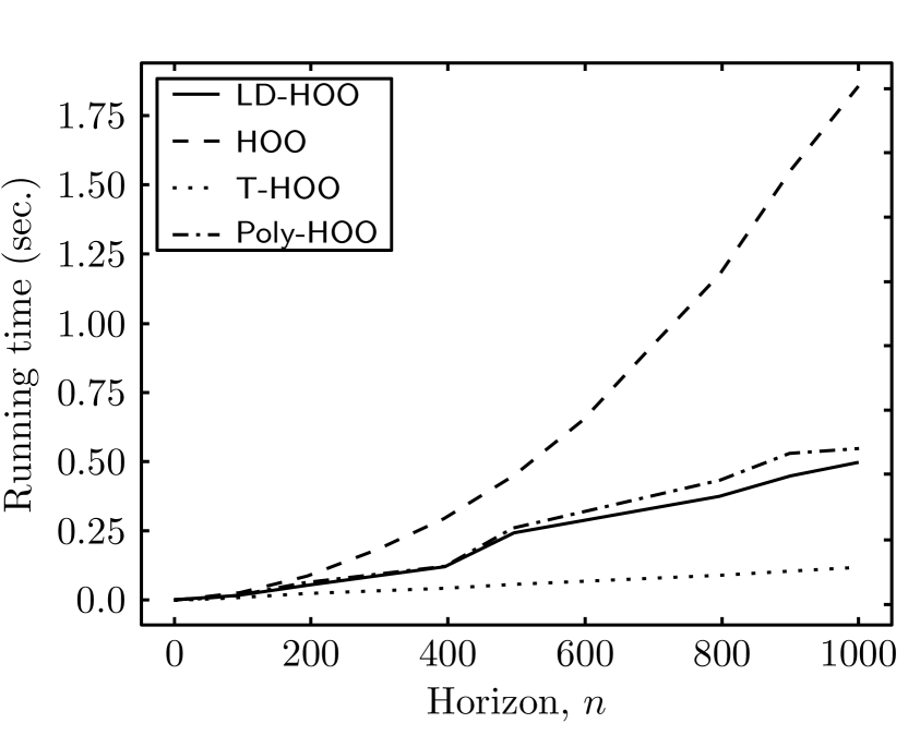
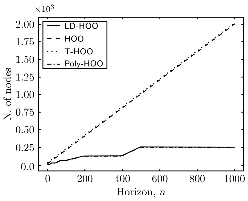
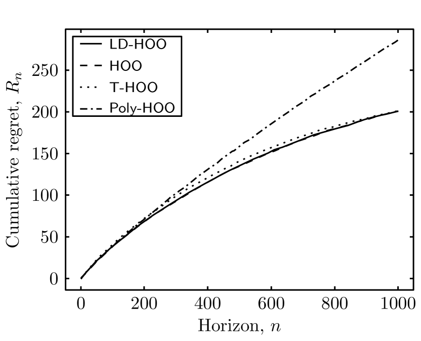
In our tests, we use a mean reward function f(x)=12(sin(13x)sin(27x)+1)𝑓𝑥1213𝑥27𝑥1f(x)=\frac{1}{2}(\sin(13x)\sin(27x)+1). The reward received by the decision-maker at each time step is a perturbed version of f𝑓f: upon selecting an action Xtsubscript𝑋𝑡X_{t}, the decision-maker receives a reward Yt=f(Xt)+εtsubscript𝑌𝑡𝑓subscript𝑋𝑡subscript𝜀𝑡Y_{t}=f(X_{t})+\varepsilon_{t}, where ε𝜀\varepsilon is drawn from a Gaussian distribution with zero mean and a standard deviation of 0.050.050.05. We set ν1=1subscript𝜈11\nu_{1}=1 and ρ=0.25𝜌0.25\rho=0.25 for all algorithms. For LD-HOO we set H^=logn^𝐻𝑛\hat{H}=\lceil\log n\rceil.111Even though our selected value for H^^𝐻\hat{H} does not verify the conditions in Corollary 1, it empirically performed well and, as such, was used in our experiments. We compare in Fig. 3 the performance of the 4 methods, as we vary the horizon between n=10𝑛10n=10 and n=1,000𝑛1000n=1,000. The results portrayed are averages of 101010 independent runs.

Refer to caption
(a) Running time.
Refer to caption
(b) Number of nodes in the partition tree.
Refer to caption
(c) Cumulative regret.
Figure 3: Performance of all HOO-based algorithms in terms of time, space and regret, as a function of the horizon, n𝑛n.

Our results are in accordance with our theoretical analysis. As seen in Figs. 3(a) and 3(b), HOO is the most computationally demanding algorithm, both in terms of time and in terms of the number of nodes. LD-HOO is similar to Poly-HOO in terms of computational complexity but, as seen in Fig. 3(c), it outperforms Poly-HOO in terms of cumulative regret. Finally, LD-HOO is similar to T-HOO in terms of regret; T-HOO exhibits a superior running time, but a worse number of nodes (the line of T-HOO in Fig. 3(b) overlaps that of HOO).

The conclusion from our empirical results is that, overall, LD-HOO achieves similar or better performance than the other algorithms. The only exception is in terms of running time, where T-HOO is noticeably faster. However, since our ultimate goal is to use our algorithm in the context of MCTS, T-HOO is not an option, since it is not an anytime algorithm [4].

4 Monte Carlo Tree Search using LD-HOO

We are now in position to introduce LD-HOOT (or LD-HOO for trees), where we combine Monte Carlo tree search with LD-HOO. We consider Markov decision problems (MDPs) where, at each step, the agent/decision-maker observes the current state of the MDP, Stsubscript𝑆𝑡S_{t}, and must select an action, Xtsubscript𝑋𝑡X_{t}, that maximizes the total discounted reward, as defined in (1). Like standard MCTS algorithms, at each step t𝑡t LD-HOOT builds a tree representation of the MDP similar to that in Fig. 1. To traverse the tree, each state node s𝑠s is treated as a multi-armed bandit problem, and an action is selected using LD-HOO. When computation time is over, LD-HOOT returns the action selected by LD-HOO at the root node (line 22 of Algorithm 1).
Refer to caption
(a) The cart pole environment.
Refer to caption
(b) The inverted pendulum environment.
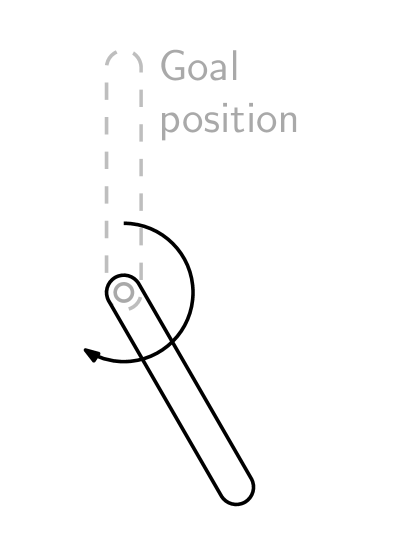
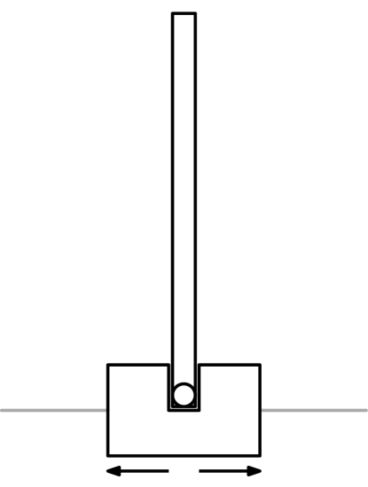
Figure 4: Illustration of the two environments used to evaluate LD-HOOT. The black arrows illustrate the control available: in the cart-pole scenario, the control is performed by applying a force to the cart. In the inverted pendulum, the control is performed by applying a force to the pendulum.

To assess the applicability of LD-HOOT, we tested the algorithm in two control problems from the literature. We used benchmark environments from OpenAI’s Gym [2], namely CartPole-v1 and Pendulum-v0, as well as the modified version of cart-pole with increased gravity of Mao et al. [9]. In the two cart-pole scenarios, the pole is initialized close to the equilibrium position, and the role of the agent is to control the cart to keep the pole (approximately) vertical. In the inverted pendulum scenario, the pendulum is initialized in an arbitrary position above the horizontal line with (possible) non-zero initial velocity, and the role of the agent is to balance the pole to the vertical position.

We used ν1=4subscript𝜈14\nu_{1}=4, ρ=0.25𝜌0.25\rho=0.25 and allowed LD-HOOT to have a lookahead limit of D=50𝐷50D=50 actions. In all scenarios, we set H^=logn^𝐻𝑛\hat{H}=\lceil\log n\rceil. In the cart-pole scenario, the agent interacted with the environment for a total of T=150𝑇150T=150 time steps. At each time step, the action of the agent was computed using n=100𝑛100n=100 iterations of the planner. In contrast, in the inverted pendulum scenario, the agent interacted with the environment for a total of T=100𝑇100T=100 time steps. However, since the environment is more difficult, each action was computed from n=100,400𝑛100400n=100,400 iterations of the planner to establish the impact of the increased n𝑛n in each of the algorithms. The number of actions executed in each environment permits a comparison with the benchmark results in Open AI Gym [12]. We normalized the rewards to the interval [0,1]01[0,1] to allow an easy comparison with the number of actions executed since, in this case, that is (potentially) the maximum cumulative reward that could be obtained.

Table 1: Average sum of rewards obtained in the four test scenarios.
Cart Pole Cart Pole IG Inverted Pendulum
n𝑛n 100 100 100 400
LD-HOOT 150.0±0.0plus-or-minus150.00.0150.0\pm 0.0 150.0±0.0plus-or-minus150.00.0150.0\pm 0.0 82.46±10.40plus-or-minus82.4610.4082.46\pm 10.40 84.36±9.00plus-or-minus84.369.0084.36\pm 9.00
HOOT 150.0±0.0plus-or-minus150.00.0150.0\pm 0.0 150.0±0.0plus-or-minus150.00.0150.0\pm 0.0 81.23±13.41plus-or-minus81.2313.4181.23\pm 13.41 81.21±11.45plus-or-minus81.2111.4581.21\pm 11.45
POLY-HOOT 150.0±0.0plus-or-minus150.00.0150.0\pm 0.0 150.0±0.0plus-or-minus150.00.0150.0\pm 0.0 82.40±11.24plus-or-minus82.4011.2482.40\pm 11.24 84.56±8.79plus-or-minus84.568.7984.56\pm 8.79

Table 1 compares the performance of LD-HOOT against that of HOOT [8] and Poly-HOOT [9], the MCTS extensions of HOO and Poly-HOO, respectively. For each algorithm, we report the sum of rewards obtained averaged over 101010 independent trials, each with a different randomly selected initial state (but the same across algorithms). The only exception are the results obtained in the Inverted Pendulum with n=100𝑛100n=100, were the number of trials was 303030. The differences in variance observed with different n𝑛n in the Inverted Pendulum tests are likely due to the discrepancy in the number of trials and, consequently, the usage of different initial states. Even though just slightly, HOOT is the only of the 3 algorithms that performed worse when running for a longer period. On the other hand, both LD-HOOT and Poly-HOOT accrued rewards over 2%percent22\% larger in this scenario, thus evidencing a superior performance against their predecessor (HOOT). As seen in Table 1, all three algorithms perform optimally in the two cart-pole scenarios (dubbed Cart Pole and Cart Pole ig). Even with increased gravity, all algorithms were able to maintain the pole approximately vertical. In contrast, in the inverted pendulum scenario LD-HOOT outperforms HOOT, and performs similarly to Poly-HOOT. It is also noteworthy that, according to Open AI’s leaderboard [12], the best performing algorithm in this scenario obtained an average cumulative reward of 92.4592.4592.45. Our results are close but, due to the large variance, it is not possible to assert whether the differences are significative or not.

Table 2: Average running time (in seconds) required to plan a single action, for different values of n𝑛n and H^^𝐻\hat{H}.
nH^conditional𝑛^𝐻n\mid\hat{H} 1005conditional1005100\mid 5 4006conditional4006400\mid 6 10007conditional100071000\mid 7
LD-HOOT 1.14±0.07plus-or-minus1.140.071.14\pm 0.07 4.51±0.06plus-or-minus4.510.064.51\pm 0.06 11.88±0.05plus-or-minus11.880.0511.88\pm 0.05
HOOT 1.06±0.04plus-or-minus1.060.041.06\pm 0.04 4.72±0.01plus-or-minus4.720.014.72\pm 0.01 15.15±2.55plus-or-minus15.152.5515.15\pm 2.55
POLY-HOOT 1.15±0.03plus-or-minus1.150.031.15\pm 0.03 4.90±0.21plus-or-minus4.900.214.90\pm 0.21 12.76±0.15plus-or-minus12.760.1512.76\pm 0.15

Table 2 reports the running time for the three algorithms for different values of n𝑛n and H^^𝐻\hat{H}, when planning a single action. The results again correspond to averages over 10 independent trials. Our results confirm that LD-HOOT is faster than HOOT, which was expected since LD-HOO is also faster than HOO. When n=100𝑛100n=100 and H^=5^𝐻5\hat{H}=5, HOOT was marginally faster, but given the small times considered it is possible that the differences may be due to other processes that are being run at the same time. LD-HOOT is also faster than Poly-HOOT in all settings considered, but differences were smaller.

Summarizing, LD-HOOT outperforms HOOT in both metrics considered, and is slightly faster than Poly-HOOT, although attaining similar cumulative rewards.

5 Conclusion

In this work, we contributed LD-HOO, a novel algorithm for stochastic multi-armed bandit problems with a continuous action spaces. We provided a regret analysis for LD-HOO and establish that, under mild conditions, LD-HOO exhibits an asymptotic regret bound similar to that of other algorithms in the literature, while incurring in smaller computational costs. Our analysis was then complemented by an empirical study, in which we show that LD-HOO generally outperforms similar algorithms.

We then propose LD-HOOT, a Monte Carlo tree search algorithm that uses LD-HOO to drive the expansion of the search tree. We tested LD-HOOT in several optimal control problems from the literature, and the results show that LD-HOO can be successfully used within MCTS to address optimal control problems with continuous actions spaces. Additionally, our results show that LD-HOOT is competitive with existing algorithms in terms of performance, while being computationally more efficient.

An interesting line for future research is to build on the results presented herein—namely Theorem 3.1—to establish the consistence of LD-HOOT in the sense that the probability of selecting the optimal action can be made to converge to 1 as the number of samples grows to infinity. Such results exist for MCTS with finite action spaces [7], and we conjecture that a similar line of proof could be used to establish similar guarantees for LD-HOOT.

6 Acknowledgments

This work was partially supported by national funds through FCT, Fundação para a Ciência e a Tecnologia, under project UIDB/50021/2020.

References

  • [1] Auer, P., Cesa-Bianchi, N., Fischer, P.: Finite-time analysis of the multiarmed bandit problem. Machine Learning 47, 235–256 (2002)
  • [2] Brockman, G., Cheung, V., Pettersson, L., Schneider, J., Schulman, J., Tang, J., Zaremba, W.: OpenAI Gym. CoRR abs/1606.01540 (2016)
  • [3] Browne, C., Powley, E., Whitehouse, D., Lucas, S., Cowling, P., Rohlfshagen, P., Tavener, S., Perez, D., Samothrakis, S., Colton, S.: A survey of Monte Carlo tree search methods. IEEE Trans. Computational Intelligence and AI in Games 4(1), 1–43 (2012)
  • [4] Bubeck, S., Munos, R., Stoltz, G., Szepesvári, C.: X𝑋X-armed bandits. J. Machine Learning Res. 12, 1655–1695 (2011)
  • [5] Bubeck, S., Stoltz, G., Szepesvári, C., Munos, R.: Online optimization in X𝑋X-armed bandits. In: Adv. Neural Information Processing Systems 21. pp. 201–208 (2009)
  • [6] Kearns, M., Mansour, Y., Ng, A.: A sparse sampling algorithm for near-optimal planning in large Markovian decision processes. In: Proc. 16th Int. Joint Conf. Artificial Intelligence. pp. 1324–1331 (1999)
  • [7] Kocsis, L., Szepesvári, C.: Bandit based Monte-Carlo planning. In: Proc. 17th European Conf. Machine Learning. pp. 282–293 (2006)
  • [8] Mansley, C., Weinstein, A., Littman, M.: Sample-based planning for continuous action Markov decision processes. In: Proc. 21st Int. Conf. Automated Planning and Scheduling. pp. 335–338 (2011)
  • [9] Mao, W., Zhang, K., Xie, Q., Basar, T.: Poly-HOOT: Monte-Carlo planning in continuous space MDPs with non-asymptotic analysis. In: Adv. Neural Information Proc. Systems 33. pp. 4549–4559 (2020)
  • [10] Munos, R.: Optimistic optimization of a deterministic function without the knowledge of its smoothness. In: Adv. Neural Information Processing Systems 24. pp. 783–791 (2011)
  • [11] Munos, R.: From bandits to Monte-Carlo tree search: The optimistic principle applied to optimization and planning. Foundations and Trends in Machine Learning 7(1), 1–129 (2014)
  • [12] Open AI: Open AI Gym’s Leaderboard
  • [13] Puterman, M.: Markov Decision Processes: Discrete Stochastic Dynamic Programming. John Wiley & Sons (2005)
  • [14] Schrittwieser, J., Antonoglou, I., Hubert, T., Simonyan, K., Sifre, L., Schmitt, S., Guez, A., Lockhart, E., Hassabis, D., Graepel, T., Lillicrap, T., Silver, D.: Mastering Atari, Go, chess and Shogi by planning with a learned model. Nature 588, 604–609 (2020)
  • [15] Silver, D., Huang, A., Maddison, C., Guez, A., Sifre, L., Driessche, G., Schrittwieser, J., Antonoglou, I., Panneershelvam, V., Lanctot, M., Dieleman, S., Grewe, D., Nham, J., Kalchbrenner, N., Sutskever, I., Lillicrap, T., Leach, M., Kavukcuoglu, K., Graepel, T., Hassabis, D.: Mastering the game of Go with deep neural networks and tree search. Nature 529, 484–489 (2016)
  • [16] Silver, D., Hubert, T., Schrittwieser, J., Antonoglou, I., Lai, M., Guez, A., Lanctot, M., Laurent, S., Kumaran, D., Graepel, T., Lillicrap, T., Simonyan, K., Hassabis, D.: A general reinforcement learning algorithm that masters chess, Shogi, and Go through self-play. Science 362(6419), 1140–1144 (2018)
  • [17] Silver, D., Schrittwieser, J., Simonyan, K., Antonoglou, I., Huang, A., Guez, A., Hubert, T., Baker, L., Lai, M., Bolton, A., Chen, Y., Lillicrap, T., Hui, F., Sifre, L., van den Driessche, G., Graepel, T., Hassabis, D.: Mastering the game of Go without human knowledge. Nature 550, 354–359 (2017)

Limited depth bandit-based strategy for Monte Carlo planning in continuous action spaces

Supplementary material for paper n. 923

Appendix 0.A Proof of Theorem 1

The proof follows the structure of the proof sketch provided in the manuscript, and is also based on the analysis of HOO found in the work of Bubeck et al [4]. Before dwelling into the proof, we introduce some auxiliary results.

0.A.1 Auxiliary results

We define the regret of a node (h,i)𝒯n𝑖subscript𝒯𝑛(h,i)\in\mathcal{T}_{n} as

rh,i=f(x)supx𝒳h,if(x).subscript𝑟𝑖𝑓superscript𝑥subscriptsupremum𝑥subscript𝒳𝑖𝑓𝑥r_{h,i}=f(x^{*})-\sup_{x\in\mathcal{X}_{h,i}}f(x).

Fix an optimal path (0,0)(1,i1)(H^,iH^)001subscriptsuperscript𝑖1^𝐻subscriptsuperscript𝑖^𝐻(0,0)\to(1,i^{*}_{1})\to\ldots\to(\hat{H},i^{*}_{\hat{H}}), where (h,ih)subscriptsuperscript𝑖(h,i^{*}_{h}) is a child of (h1,ih1)1superscriptsubscript𝑖1(h-1,i_{h-1}^{*}) and ihsubscriptsuperscript𝑖i^{*}_{h} is such that rh,ih=0subscript𝑟subscriptsuperscript𝑖0r_{h,i^{*}_{h}}=0. Define the set

𝒞^(h,i)={c𝒯n𝒳c𝒳h,i},^𝒞𝑖conditional-set𝑐subscript𝒯𝑛subscript𝒳𝑐subscript𝒳𝑖\hat{\mathcal{C}}(h,i)=\left\{c\in\mathcal{T}_{n}\mid\mathcal{X}_{c}\subset\mathcal{X}_{h,i}\right\},

i.e., 𝒞^(h,i)^𝒞𝑖\hat{\mathcal{C}}(h,i) is the set containing node (h,i)𝑖(h,i) and all its descendants. The next lemma bounds the number of times that a suboptimal node (h,i)𝑖(h,i) is selected up to iteration n𝑛n. Having a bound for the expected number of times that a suboptimal node can be played is crucial to bound the expected cumulative regret.

Lemma 1.

Let (h0,i0)subscript0subscript𝑖0(h_{0},i_{0}) be a suboptimal node (i.e., a node not in the path above), and let k𝑘k be the largest integer such that 0kh010𝑘subscript010\leq k\leq h_{0}-1 and (k,ik)𝑘subscriptsuperscript𝑖𝑘(k,i^{*}_{k}) is in the path from (0,0)00(0,0) to (h0,i0)subscript0subscript𝑖0(h_{0},i_{0}).222The extreme case is k=0𝑘0k=0. Then for all integers z0𝑧0z\geq 0, we have

𝔼[Th0,i0(n)]z+t=z+1n[(uh,ih(t)f(x) for some h{k+1,,H^}) or (Th0,i0(t)>z and uh0,i0(t)>f(x))].𝔼delimited-[]subscript𝑇subscript0subscript𝑖0𝑛𝑧superscriptsubscript𝑡𝑧1𝑛delimited-[]subscript𝑢subscriptsuperscript𝑖𝑡𝑓superscript𝑥 for some 𝑘1^𝐻 or subscript𝑇subscript0subscript𝑖0𝑡𝑧 and subscript𝑢subscript0subscript𝑖0𝑡𝑓superscript𝑥\mathbb{E}\left[T_{h_{0},i_{0}}(n)\right]\leq z+\sum_{t=z+1}^{n}\mathbb{P}\Big{[}\big{(}u_{h,i^{*}_{h}}(t)\leq f(x^{*})\text{ for some }h\in\{k+1,\ldots,\hat{H}\}\big{)}\\ \text{ or }\big{(}T_{h_{0},i_{0}}(t)>z\text{ and }u_{h_{0},i_{0}}(t)>f(x^{*})\big{)}\Big{]}.
Proof.

Let (ht,it)subscript𝑡subscript𝑖𝑡(h_{t},i_{t}) denote the node selected by LD-HOO at some time step t𝑡t. If (ht,it)𝒞^(h0,i0)subscript𝑡subscript𝑖𝑡^𝒞subscript0subscript𝑖0(h_{t},i_{t})\in\hat{\mathcal{C}}(h_{0},i_{0}), then at depth k𝑘k there is a node (k+1,i)𝒞(k,ik)𝑘1𝑖𝒞𝑘subscriptsuperscript𝑖𝑘(k+1,i)\in\mathcal{C}(k,i^{*}_{k}) which, by definition of k𝑘k, is different from (k+1,ik+1)𝑘1subscriptsuperscript𝑖𝑘1(k+1,i^{*}_{k+1}).

By construction, the b𝑏b-value of a node is greater than or equal to that of its parent node. Hence, since node (k+1,i)𝑘1𝑖(k+1,i) was selected instead of (k+1,ik+1)𝑘1subscriptsuperscript𝑖𝑘1(k+1,i^{*}_{k+1}), then bk+1,ik+1(t)bk+1,i(t)bh0,i0(t)subscript𝑏𝑘1subscriptsuperscript𝑖𝑘1𝑡subscript𝑏𝑘1𝑖𝑡subscript𝑏subscript0subscript𝑖0𝑡b_{k+1,i^{*}_{k+1}}(t)\leq b_{k+1,i}(t)\leq b_{h_{0},i_{0}}(t). This implies, again by construction, that bh0,i0(t)uh0,i0(t)subscript𝑏subscript0subscript𝑖0𝑡subscript𝑢subscript0subscript𝑖0𝑡b_{h_{0},i_{0}}(t)\leq u_{h_{0},i_{0}}(t) and bk+1,ik+1(t)uh0,i0(t)subscript𝑏𝑘1subscriptsuperscript𝑖𝑘1𝑡subscript𝑢subscript0subscript𝑖0𝑡b_{k+1,i^{*}_{k+1}}(t)\leq u_{h_{0},i_{0}}(t). Putting everything together, we have

(ht,it)𝒞^(h0,i0)uh0,i0(t)bk+1,ik+1(t)(uh0,i0(t)>f(x) or bk+1,ik+1(t)f(x)).subscript𝑡subscript𝑖𝑡^𝒞subscript0subscript𝑖0subscript𝑢subscript0subscript𝑖0𝑡subscript𝑏𝑘1subscriptsuperscript𝑖𝑘1𝑡subscript𝑢subscript0subscript𝑖0𝑡𝑓superscript𝑥 or subscript𝑏𝑘1subscriptsuperscript𝑖𝑘1𝑡𝑓superscript𝑥\begin{split}(h_{t},i_{t})\in\hat{\mathcal{C}}(h_{0},i_{0})&\Rightarrow u_{h_{0},i_{0}}(t)\geq b_{k+1,i^{*}_{k+1}}(t)\\ &\Rightarrow\big{(}u_{h_{0},i_{0}}(t)>f(x^{*})\text{ or }b_{k+1,i^{*}_{k+1}}(t)\leq f(x^{*})\big{)}.\end{split} (13)

To see why the last implication holds, suppose that uh0,i0(t)bk+1,ik+1(t)subscript𝑢subscript0subscript𝑖0𝑡subscript𝑏𝑘1subscriptsuperscript𝑖𝑘1𝑡u_{h_{0},i_{0}}(t)\geq b_{k+1,i^{*}_{k+1}}(t). Then, if uh0,i0(t)f(x)subscript𝑢subscript0subscript𝑖0𝑡𝑓superscript𝑥u_{h_{0},i_{0}}(t)\leq f(x^{*}), it follows that bk+1,ik+1(t)uh0,i0(t)f(x)subscript𝑏𝑘1subscriptsuperscript𝑖𝑘1𝑡subscript𝑢subscript0subscript𝑖0𝑡𝑓superscript𝑥b_{k+1,i^{*}_{k+1}}(t)\leq u_{h_{0},i_{0}}(t)\leq f(x^{*}), and the conclusion follows.

We also have that

bk+1,ik+1(t)f(x)(uk+1,ik+1(t)f(x) or bk+2,ik+2(t)f(x)).subscript𝑏𝑘1subscriptsuperscript𝑖𝑘1𝑡𝑓superscript𝑥subscript𝑢𝑘1subscriptsuperscript𝑖𝑘1𝑡𝑓superscript𝑥 or subscript𝑏𝑘2subscriptsuperscript𝑖𝑘2𝑡𝑓superscript𝑥b_{k+1,i^{*}_{k+1}}(t)\leq f(x^{*})\Rightarrow\big{(}u_{k+1,i^{*}_{k+1}}(t)\leq f(x^{*})\text{ or }b_{k+2,i^{*}_{k+2}}(t)\leq f(x^{*})\big{)}. (14)

To see why the implication in (14) holds, suppose that bk+1,ik+1f(x)subscript𝑏𝑘1subscriptsuperscript𝑖𝑘1𝑓superscript𝑥b_{k+1,i^{*}_{k+1}}\leq f(x^{*}) holds. Then, if uk+1,ik+1(t)>f(x)subscript𝑢𝑘1subscriptsuperscript𝑖𝑘1𝑡𝑓superscript𝑥u_{k+1,i^{*}_{k+1}}(t)>f(x^{*}), the child of (k+1,ik+1)𝑘1subscriptsuperscript𝑖𝑘1(k+1,i^{*}_{k+1}) with maximum b𝑏b-value, say (k+2,j)𝑘2𝑗(k+2,j), satisfies bk+2,j(t)f(x)subscript𝑏𝑘2𝑗𝑡𝑓superscript𝑥b_{k+2,j}(t)\leq f(x^{*}) since, by construction,

bk+1,ik+1(t)=min{uk+1,ik+1(t),bk+2,j(t)}.subscript𝑏𝑘1subscriptsuperscript𝑖𝑘1𝑡subscript𝑢𝑘1subscriptsuperscript𝑖𝑘1𝑡subscript𝑏𝑘2𝑗𝑡b_{k+1,i^{*}_{k+1}}(t)=\min\left\{u_{k+1,i^{*}_{k+1}}(t),b_{k+2,j}(t)\right\}.

Then, we must have bk+2,ik+2(t)f(x)subscript𝑏𝑘2subscriptsuperscript𝑖𝑘2𝑡𝑓superscript𝑥b_{k+2,i^{*}_{k+2}}(t)\leq f(x^{*}) and the conclusion follows.

Finally, since LD-HOO does not expand nodes beyond depth H^^𝐻\hat{H}, we have that

bH^,iH^(t)=uH^,iH^(t).subscript𝑏^𝐻subscriptsuperscript𝑖^𝐻𝑡subscript𝑢^𝐻subscriptsuperscript𝑖^𝐻𝑡b_{\hat{H},i^{*}_{\hat{H}}}(t)=u_{\hat{H},i^{*}_{\hat{H}}}(t). (15)

Unfolding (14) and combining with (15) yields

bk+1,ik+1(t)f(x)subscript𝑏𝑘1subscriptsuperscript𝑖𝑘1𝑡𝑓superscript𝑥\displaystyle b_{k+1,i^{*}_{k+1}}(t)\leq f(x^{*})
(uk+1,ik+1(t)f(x) or bk+2,ik+2(t)f(x))absentsubscript𝑢𝑘1subscriptsuperscript𝑖𝑘1𝑡𝑓superscript𝑥 or subscript𝑏𝑘2subscriptsuperscript𝑖𝑘2𝑡𝑓superscript𝑥\displaystyle\Rightarrow\big{(}u_{k+1,i^{*}_{k+1}}(t)\leq f(x^{*})\text{ or }b_{k+2,i^{*}_{k+2}}(t)\leq f(x^{*})\big{)}
(uk+1,ik+1(t)f(x) or uk+2,ik+2(t)f(x) or bk+3,ik+3(t)f(x))absentsubscript𝑢𝑘1subscriptsuperscript𝑖𝑘1𝑡𝑓superscript𝑥 or subscript𝑢𝑘2subscriptsuperscript𝑖𝑘2𝑡𝑓superscript𝑥 or subscript𝑏𝑘3subscriptsuperscript𝑖𝑘3𝑡𝑓superscript𝑥\displaystyle\Rightarrow\big{(}u_{k+1,i^{*}_{k+1}}(t)\leq f(x^{*})\text{ or }u_{k+2,i^{*}_{k+2}}(t)\leq f(x^{*})\text{ or }b_{k+3,i^{*}_{k+3}}(t)\leq f(x^{*})\big{)}
\displaystyle\vdots
(uk+1,ik+1(t)f(x) or uk+2,ik+2(t)f(x) or  or uH^,iH^(t)f(x)).absentsubscript𝑢𝑘1subscriptsuperscript𝑖𝑘1𝑡𝑓superscript𝑥 or subscript𝑢𝑘2subscriptsuperscript𝑖𝑘2𝑡𝑓superscript𝑥 or  or subscript𝑢^𝐻subscriptsuperscript𝑖^𝐻𝑡𝑓superscript𝑥\displaystyle\Rightarrow\big{(}u_{k+1,i^{*}_{k+1}}(t)\leq f(x^{*})\text{ or }u_{k+2,i^{*}_{k+2}}(t)\leq f(x^{*})\text{ or }\ldots\text{ or }u_{\hat{H},i^{*}_{\hat{H}}}(t)\leq f(x^{*})\big{)}.

Combining with (13), we finally get

(ht,it)𝒞^(h0,i0)(uh0,i0(t)>f(x) or uk+1,ik+1(t)f(x) or  or uH^,iH^(t)f(x).(h_{t},i_{t})\in\hat{\mathcal{C}}(h_{0},i_{0})\\ \Rightarrow\big{(}u_{h_{0},i_{0}}(t)>f(x^{*})\text{ or }u_{k+1,i^{*}_{k+1}}(t)\leq f(x^{*})\text{ or }\ldots\text{ or }u_{\hat{H},i^{*}_{\hat{H}}}(t)\leq f(x^{*}). (16)

For any integer z0𝑧0z\geq 0,

Th0,i0(n)subscript𝑇subscript0subscript𝑖0𝑛\displaystyle T_{h_{0},i_{0}}(n)
=t=1n𝕀[(ht,it)𝒞^(h0,i0)]absentsuperscriptsubscript𝑡1𝑛𝕀delimited-[]subscript𝑡subscript𝑖𝑡^𝒞subscript0subscript𝑖0\displaystyle=\sum_{t=1}^{n}\mathbb{I}\left[(h_{t},i_{t})\in\hat{\mathcal{C}}(h_{0},i_{0})\right]
=t=1n𝕀[(ht,it)𝒞^(h0,i0),Th0,i0(t)z]+t=1n𝕀[(ht,it)𝒞^(h0,i0),Th0,i0(t)>z]absentsuperscriptsubscript𝑡1𝑛𝕀delimited-[]formulae-sequencesubscript𝑡subscript𝑖𝑡^𝒞subscript0subscript𝑖0subscript𝑇subscript0subscript𝑖0𝑡𝑧superscriptsubscript𝑡1𝑛𝕀delimited-[]formulae-sequencesubscript𝑡subscript𝑖𝑡^𝒞subscript0subscript𝑖0subscript𝑇subscript0subscript𝑖0𝑡𝑧\displaystyle=\sum_{t=1}^{n}\mathbb{I}\left[(h_{t},i_{t})\in\hat{\mathcal{C}}(h_{0},i_{0}),T_{h_{0},i_{0}}(t)\leq z\right]+\sum_{t=1}^{n}\mathbb{I}\left[(h_{t},i_{t})\in\hat{\mathcal{C}}(h_{0},i_{0}),T_{h_{0},i_{0}}(t)>z\right]
z+t=z+1n𝕀[(ht,it)𝒞^(h0,i0),Th0,i0(t)>z].absent𝑧superscriptsubscript𝑡𝑧1𝑛𝕀delimited-[]formulae-sequencesubscript𝑡subscript𝑖𝑡^𝒞subscript0subscript𝑖0subscript𝑇subscript0subscript𝑖0𝑡𝑧\displaystyle\leq z+\sum_{t=z+1}^{n}\mathbb{I}\left[(h_{t},i_{t})\in\hat{\mathcal{C}}(h_{0},i_{0}),T_{h_{0},i_{0}}(t)>z\right].

Taking the expectation and replacing (16), we finally get

𝔼[Th0,i0(n)]𝔼delimited-[]subscript𝑇subscript0subscript𝑖0𝑛\displaystyle\mathbb{E}\left[T_{h_{0},i_{0}}(n)\right]
z+t=z+1n[(ht,it)𝒞^(h0,i0),Th0,i0(t)>z]absent𝑧superscriptsubscript𝑡𝑧1𝑛delimited-[]formulae-sequencesubscript𝑡subscript𝑖𝑡^𝒞subscript0subscript𝑖0subscript𝑇subscript0subscript𝑖0𝑡𝑧\displaystyle\leq z+\sum_{t=z+1}^{n}\mathbb{P}\left[(h_{t},i_{t})\in\hat{\mathcal{C}}(h_{0},i_{0}),T_{h_{0},i_{0}}(t)>z\right]
z+t=z+1n[Th0,i0(t)>z and (uh,ih(t)f(x) for some h{k+1,,H^})\displaystyle\leq z+\sum_{t=z+1}^{n}\mathbb{P}\Big{[}T_{h_{0},i_{0}}(t)>z\text{ and }\big{(}u_{h,i^{*}_{h}}(t)\leq f(x^{*})\text{ for some }h\in\{k+1,\ldots,\hat{H}\}\big{)}
 or (Th0,i0(t)>z and uh0,i0(t)>f(x))]\displaystyle\hskip 156.49014pt\text{ or }\big{(}T_{h_{0},i_{0}}(t)>z\text{ and }u_{h_{0},i_{0}}(t)>f(x^{*})\big{)}\Big{]}
z+t=z+1n[(uh,ih(t)f(x) for some h{k+1,,H^})\displaystyle\leq z+\sum_{t=z+1}^{n}\mathbb{P}\Big{[}\big{(}u_{h,i^{*}_{h}}(t)\leq f(x^{*})\text{ for some }h\in\{k+1,\ldots,\hat{H}\}\big{)}
 or (Th0,i0(t)>z and uh0,i0(t)>f(x))].\displaystyle\hskip 156.49014pt\text{ or }\big{(}T_{h_{0},i_{0}}(t)>z\text{ and }u_{h_{0},i_{0}}(t)>f(x^{*})\big{)}\Big{]}.

The proof is thus complete. ∎

The next lemmata are established by Bubeck et al. [4] and are provided without proof.

Lemma 2.

If Assumptions 1 through 3 hold then, for all optimal nodes (h,i)𝑖(h,i) and integers t>0𝑡0t>0,

[uh,i(t)f(x)]1t3.delimited-[]subscript𝑢𝑖𝑡𝑓superscript𝑥1superscript𝑡3\mathbb{P}\left[u_{h,i}(t)\leq f(x^{*})\right]\leq\frac{1}{t^{3}}.
Lemma 3.

Suppose that Assumptions 1 through 3 hold. Then, for all integers tn𝑡𝑛t\leq n, all suboptimal nodes (h,i)𝑖(h,i) such that rh,i>ν1ρhsubscript𝑟𝑖subscript𝜈1superscript𝜌r_{h,i}>\nu_{1}\rho^{h}, and for all integers z𝑧z such that

z8logn(rh,iν1ρh)2,𝑧8𝑛superscriptsubscript𝑟𝑖subscript𝜈1superscript𝜌2z\geq\frac{8\log n}{(r_{h,i}-\nu_{1}\rho^{h})^{2}},

it holds that

[uh,i(t)>f(x) and Th,i(t)>z]tn4.delimited-[]subscript𝑢𝑖𝑡𝑓superscript𝑥 and subscript𝑇𝑖𝑡𝑧𝑡superscript𝑛4\mathbb{P}\left[u_{h,i}(t)>f(x^{*})\text{ and }T_{h,i}(t)>z\right]\leq\frac{t}{n^{4}}.
Lemma 4.

Suppose that Assumptions 1 through 3 hold. If, for a node (h,i)𝑖(h,i), rh,icν1ρhsubscript𝑟𝑖𝑐subscript𝜈1superscript𝜌r_{h,i}\leq c\nu_{1}\rho^{h}, then

𝒳h,i𝒳max{2c,c+1}ν1ρh.subscript𝒳𝑖subscript𝒳2𝑐𝑐1subscript𝜈1superscript𝜌\mathcal{X}_{h,i}\subset\mathcal{X}_{\max\{2c,c+1\}\nu_{1}\rho^{h}}. (17)

The next result provides an upper bound for the number of visits to a suboptimal node (h,i)𝑖(h,i).

Lemma 5.

If Assumptions 1 through 3 hold then, for all suboptimal nodes (h,i)𝑖(h,i) with rh,i>ν1ρhsubscript𝑟𝑖subscript𝜈1superscript𝜌r_{h,i}>\nu_{1}\rho^{h} and n1𝑛1n\geq 1,

𝔼[Th,i(n)]8logn(rh,iν1ρh)2+2(H^+1).𝔼delimited-[]subscript𝑇𝑖𝑛8𝑛superscriptsubscript𝑟𝑖subscript𝜈1superscript𝜌22^𝐻1\mathbb{E}\left[T_{h,i}(n)\right]\leq\frac{8\log n}{(r_{h,i}-\nu_{1}\rho^{h})^{2}}+2(\hat{H}+1).
Proof.

Let (h0,i0)subscript0subscript𝑖0(h_{0},i_{0}) denote an arbitrary suboptimal node. Taking

z=8logn(rh0,i0ν1ρh0)2𝑧8𝑛superscriptsubscript𝑟subscript0subscript𝑖0subscript𝜈1superscript𝜌subscript02z=\left\lceil\frac{8\log n}{(r_{h_{0},i_{0}}-\nu_{1}\rho^{h_{0}})^{2}}\right\rceil

in Lemma 1, we get

𝔼[Th0,i0(n)]8logn(rh,iν1ρh)2+1+t=z+1n([Th0,i0(t)>z and uh0,i0(t)>f(x)]+h=1H^[uh,ih(t)f(x)]).𝔼delimited-[]subscript𝑇subscript0subscript𝑖0𝑛8𝑛superscriptsubscript𝑟𝑖subscript𝜈1superscript𝜌21superscriptsubscript𝑡𝑧1𝑛delimited-[]subscript𝑇subscript0subscript𝑖0𝑡𝑧 and subscript𝑢subscript0subscript𝑖0𝑡𝑓superscript𝑥superscriptsubscript1^𝐻delimited-[]subscript𝑢subscriptsuperscript𝑖𝑡𝑓superscript𝑥\mathbb{E}\left[T_{h_{0},i_{0}}(n)\right]\leq\frac{8\log n}{(r_{h,i}-\nu_{1}\rho^{h})^{2}}+1\\ +\sum_{t=z+1}^{n}\Big{(}\mathbb{P}\left[T_{h_{0},i_{0}}(t)>z\text{ and }u_{h_{0},i_{0}}(t)>f(x^{*})\right]+\sum_{h=1}^{\hat{H}}\mathbb{P}\left[u_{h,i^{*}_{h}}(t)\leq f(x^{*})\right]\Big{)}.

Using Lemmas 2 and 3,

𝔼[Th0,i0(n)]𝔼delimited-[]subscript𝑇subscript0subscript𝑖0𝑛\displaystyle\mathbb{E}\left[T_{h_{0},i_{0}}(n)\right] 8logn(rh,iν1ρh)2+1+t=z+1n(tn4+H^t3)absent8𝑛superscriptsubscript𝑟𝑖subscript𝜈1superscript𝜌21superscriptsubscript𝑡𝑧1𝑛𝑡superscript𝑛4^𝐻superscript𝑡3\displaystyle\leq\frac{8\log n}{(r_{h,i}-\nu_{1}\rho^{h})^{2}}+1+\sum_{t=z+1}^{n}\Big{(}\frac{t}{n^{4}}+\frac{\hat{H}}{t^{3}}\Big{)}
8logn(rh,iν1ρh)2+1+1n2+H^t=1n1t3absent8𝑛superscriptsubscript𝑟𝑖subscript𝜈1superscript𝜌211superscript𝑛2^𝐻subscriptsuperscript𝑛𝑡11superscript𝑡3\displaystyle\leq\frac{8\log n}{(r_{h,i}-\nu_{1}\rho^{h})^{2}}+1+\frac{1}{n^{2}}+\hat{H}\sum^{n}_{t=1}\frac{1}{t^{3}}
8logn(rh,iν1ρh)2+2+2H^,absent8𝑛superscriptsubscript𝑟𝑖subscript𝜈1superscript𝜌222^𝐻\displaystyle\leq\frac{8\log n}{(r_{h,i}-\nu_{1}\rho^{h})^{2}}+2+2\hat{H},

where the last inequality follows from the fact that t=1n1t3<2superscriptsubscript𝑡1𝑛1superscript𝑡32\sum_{t=1}^{n}\frac{1}{t^{3}}<2. ∎

Having proved Lemma 5, it is now possible to finalise the proof of the main result.

0.A.2 Proof of the theorem

The proof proceeds along the same four steps outlined in the manuscript. We specialize the bound in Lemma 5 to bound the number of times that suboptimal nodes in the tree are selected. The second step breaks down the value of 𝔼[Rn]𝔼delimited-[]subscript𝑅𝑛\mathbb{E}\left[R_{n}\right] into three components. The third step bounds each component of the regret individually. The fourth step wraps the proof by combining the intermediate results into a final regret bound.

We revisit some notation. For a node (h,i)𝑖(h,i) in 𝒯nsubscript𝒯𝑛\mathcal{T}_{n}, let fh,i=supx𝒳h,if(x)superscriptsubscript𝑓𝑖subscriptsupremum𝑥subscript𝒳𝑖𝑓𝑥f_{h,i}^{*}=\sup_{x\in\mathcal{X}_{h,i}}f(x), and define the set

h={(h,i)fh,if(x)2ν1ρh},subscriptconditional-set𝑖subscriptsuperscript𝑓𝑖𝑓superscript𝑥2subscript𝜈1superscript𝜌\mathcal{I}_{h}=\left\{(h,i)\mid f^{*}_{h,i}\geq f(x^{*})-2\nu_{1}\rho^{h}\right\},

i.e., hsubscript\mathcal{I}_{h} is the set of 2ν1ρh2subscript𝜈1superscript𝜌2\nu_{1}\rho^{h}-optimal nodes at depth hh. Let 𝒥hsubscript𝒥\mathcal{J}_{h} be the set of nodes at depth hh that are not in hsubscript\mathcal{I}_{h} but whose parents are in h1subscript1\mathcal{I}_{h-1}.

First step.

We start by noting that we can use Lemma 5 to bound the expected number of times that a node (h,i)𝒥h𝑖subscript𝒥(h,i)\in\mathcal{J}_{h} is played. Noting that, for these nodes, rh,i>2ν1ρhsubscript𝑟𝑖2subscript𝜈1superscript𝜌r_{h,i}>2\nu_{1}\rho^{h}, then

𝔼[Th,i(n)]8logn(2ν1ρhν1ρh)2+2(H^+1)=8lognν12ρ2h+2(H^+1).𝔼delimited-[]subscript𝑇𝑖𝑛8𝑛superscript2subscript𝜈1superscript𝜌subscript𝜈1superscript𝜌22^𝐻18𝑛superscriptsubscript𝜈12superscript𝜌22^𝐻1\mathbb{E}\left[T_{h,i}(n)\right]\leq\frac{8\log n}{(2\nu_{1}\rho^{h}-\nu_{1}\rho^{h})^{2}}+2(\hat{H}+1)=\frac{8\log n}{\nu_{1}^{2}\rho^{2h}}+2(\hat{H}+1). (18)

We can also bound the cardinality of sets hsubscript\mathcal{I}_{h}. Define

𝒰h=ch𝒳c.subscript𝒰subscript𝑐subscriptsubscript𝒳𝑐\mathcal{U}_{h}=\cup_{c\in\mathcal{I}_{h}}\mathcal{X}_{c}.

In other words, 𝒰hsubscript𝒰\mathcal{U}_{h} is the union of all cells 𝒳h,isubscript𝒳𝑖\mathcal{X}_{h,i} such that (h,i)h𝑖subscript(h,i)\in\mathcal{I}_{h}. Since, by definition, for (h,i)h𝑖subscript(h,i)\in\mathcal{I}_{h}, rh,i2ν1ρhsubscript𝑟𝑖2subscript𝜈1superscript𝜌r_{h,i}\leq 2\nu_{1}\rho^{h}, it follows from Lemma 4 (with c=2)c=2) that 𝒳h,i𝒳4ν1ρhsubscript𝒳𝑖subscript𝒳4subscript𝜈1superscript𝜌\mathcal{X}_{h,i}\subset\mathcal{X}_{4\nu_{1}\rho^{h}} and, therefore, 𝒰h𝒳4ν1ρhsubscript𝒰subscript𝒳4subscript𝜈1superscript𝜌\mathcal{U}_{h}\subset\mathcal{X}_{4\nu_{1}\rho^{h}}. But then, the cardinality of hsubscript\mathcal{I}_{h} can be bounded as

|h|𝒩(𝒰h,,ν2ρh)𝒩(𝒳4ν1ρh,,ν2ρh)=𝒩(𝒳4ν1ν2ν2ρh,,ν2ρh).subscript𝒩subscript𝒰subscript𝜈2superscript𝜌𝒩subscript𝒳4subscript𝜈1superscript𝜌subscript𝜈2superscript𝜌𝒩subscript𝒳4subscript𝜈1subscript𝜈2subscript𝜈2superscript𝜌subscript𝜈2superscript𝜌\displaystyle\left\lvert\mathcal{I}_{h}\right\rvert\leq\mathcal{N}(\mathcal{U}_{h},\ell,\nu_{2}\rho^{h})\leq\mathcal{N}(\mathcal{X}_{4\nu_{1}\rho^{h}},\ell,\nu_{2}\rho^{h})=\mathcal{N}(\mathcal{X}_{\frac{4\nu_{1}}{\nu_{2}}\nu_{2}\rho^{h}},\ell,\nu_{2}\rho^{h}).

If d𝑑d is the (4ν1/ν2,ν2)4subscript𝜈1subscript𝜈2subscript𝜈2(4\nu_{1}/\nu_{2},\nu_{2})-near-optimality dimension, by definition there is C>0𝐶0C>0 such that

|h|𝒩(𝒳4ν1ν2ν2ρh,,ν2ρh)C(ν2ρh)dsubscript𝒩subscript𝒳4subscript𝜈1subscript𝜈2subscript𝜈2superscript𝜌subscript𝜈2superscript𝜌𝐶superscriptsubscript𝜈2superscript𝜌𝑑\left\lvert\mathcal{I}_{h}\right\rvert\leq\mathcal{N}(\mathcal{X}_{\frac{4\nu_{1}}{\nu_{2}}\nu_{2}\rho^{h}},\ell,\nu_{2}\rho^{h})\leq C(\nu_{2}\rho^{h})^{-d} (19)

Second step.

We partition the nodes of 𝒯nsubscript𝒯𝑛\mathcal{T}_{n} into three disjoint sets, 𝒯1superscript𝒯1\mathcal{T}^{1}, 𝒯2superscript𝒯2\mathcal{T}^{2}, and 𝒯3superscript𝒯3\mathcal{T}^{3}, such that 𝒯1𝒯2𝒯3=𝒯nsuperscript𝒯1superscript𝒯2superscript𝒯3subscript𝒯𝑛\mathcal{T}^{1}\cup\mathcal{T}^{2}\cup\mathcal{T}^{3}=\mathcal{T}_{n}. In particular,

  • 𝒯1superscript𝒯1\mathcal{T}^{1} is the set of nodes at depth H^^𝐻\hat{H} that are 2ν1ρH^2subscript𝜈1superscript𝜌^𝐻2\nu_{1}\rho^{\hat{H}}-optimal, i.e., 𝒯1=H^superscript𝒯1subscript^𝐻\mathcal{T}^{1}=\mathcal{I}_{\hat{H}}.

  • 𝒯2superscript𝒯2\mathcal{T}^{2} is the sets of all 2ν1ρh2subscript𝜈1superscript𝜌2\nu_{1}\rho^{h}-optimal nodes, for all depths hH^^𝐻h\neq\hat{H}, i.e., 𝒯2=h=0H^1hsuperscript𝒯2superscriptsubscript0^𝐻1subscript\mathcal{T}^{2}=\cup_{h=0}^{\hat{H}-1}\mathcal{I}_{h}.

  • 𝒯3superscript𝒯3\mathcal{T}^{3} is the set set of all remaining nodes, i.e., h=1H^𝒥hsuperscriptsubscript1^𝐻subscript𝒥\cup_{h=1}^{\hat{H}}\mathcal{J}_{h} and corresponding descendant nodes.

We now define the regret Rn,ksubscript𝑅𝑛𝑘R_{n,k} of playing actions in 𝒯k,k=1,2,3formulae-sequencesuperscript𝒯𝑘𝑘123\mathcal{T}^{k},k=1,2,3, as

Rn,k=t=1n(f(x)f(Xt))𝕀[(Ht,It)𝒯k]subscript𝑅𝑛𝑘superscriptsubscript𝑡1𝑛𝑓superscript𝑥𝑓subscript𝑋𝑡𝕀delimited-[]subscript𝐻𝑡subscript𝐼𝑡superscript𝒯𝑘R_{n,k}=\sum_{t=1}^{n}(f(x^{*})-f(X_{t}))\mathbb{I}\left[(H_{t},I_{t})\in\mathcal{T}^{k}\right]

where f(Xt)𝑓subscript𝑋𝑡f(X_{t}) is the expected reward collected at time step t𝑡t given the action Xtsubscript𝑋𝑡X_{t} and (Ht,It)subscript𝐻𝑡subscript𝐼𝑡(H_{t},I_{t}) is the (random) node selected in that same time step. It follows that

𝔼[Rn]=𝔼[Rn,1]+𝔼[Rn,2]+𝔼[Rn,3].𝔼delimited-[]subscript𝑅𝑛𝔼delimited-[]subscript𝑅𝑛1𝔼delimited-[]subscript𝑅𝑛2𝔼delimited-[]subscript𝑅𝑛3\mathbb{E}\left[R_{n}\right]=\mathbb{E}\left[R_{n,1}\right]+\mathbb{E}\left[R_{n,2}\right]+\mathbb{E}\left[R_{n,3}\right]. (20)

Third step.

We now bound each of the terms in (20) to establish a bound for the total cumulative regret after n𝑛n rounds.

Starting with Rn,1subscript𝑅𝑛1R_{n,1}, in the worst case we have that

𝔼[Rn,1]4nν1ρH^.𝔼delimited-[]subscript𝑅𝑛14𝑛subscript𝜈1superscript𝜌^𝐻\mathbb{E}\left[R_{n,1}\right]\leq 4n\nu_{1}\rho^{\hat{H}}. (21)

In turn, the nodes (h,i)𝒯2𝑖superscript𝒯2(h,i)\in\mathcal{T}^{2} are 2ν1ρh2subscript𝜈1superscript𝜌2\nu_{1}\rho^{h}-optimal. This means that

𝔼[Rn,2]t=1n4ν1ρHt𝕀[(Ht,It)𝒯2]𝔼delimited-[]subscript𝑅𝑛2superscriptsubscript𝑡1𝑛4subscript𝜈1superscript𝜌subscript𝐻𝑡𝕀delimited-[]subscript𝐻𝑡subscript𝐼𝑡superscript𝒯2\mathbb{E}\left[R_{n,2}\right]\leq\sum_{t=1}^{n}4\nu_{1}\rho^{H_{t}}\mathbb{I}\left[(H_{t},I_{t})\in\mathcal{T}^{2}\right]

However, each node (h,i)𝒯2𝑖superscript𝒯2(h,i)\in\mathcal{T}^{2} is selected only once and then expanded—only nodes at depth H^^𝐻\hat{H} can be selected multiple times. As such, we can use the bound in (19) to get

𝔼[Rn,2]h=0H^14ν1ρh|h|4Cν1ν2dh=0H^1ρh(1d)𝔼delimited-[]subscript𝑅𝑛2superscriptsubscript0^𝐻14subscript𝜈1superscript𝜌subscript4𝐶subscript𝜈1superscriptsubscript𝜈2𝑑superscriptsubscript0^𝐻1superscript𝜌1𝑑\mathbb{E}\left[R_{n,2}\right]\leq\sum_{h=0}^{\hat{H}-1}4\nu_{1}\rho^{h}\left\lvert\mathcal{I}_{h}\right\rvert\leq 4C\nu_{1}\nu_{2}^{-d}\sum_{h=0}^{\hat{H}-1}\rho^{h(1-d)} (22)

Finally, let us consider the nodes in 𝒯3superscript𝒯3\mathcal{T}^{3}. Each node (h,i)𝒥h𝑖subscript𝒥(h,i)\in\mathcal{J}_{h} is the child of a node in h1subscript1\mathcal{I}_{h-1} and, as such, f(x)fh,i4ν1ρh1𝑓superscript𝑥subscriptsuperscript𝑓𝑖4subscript𝜈1superscript𝜌1f(x^{*})-f^{*}_{h,i}\leq 4\nu_{1}\rho^{h-1}. Additionally, |𝒥h|2|h1|subscript𝒥2subscript1\left\lvert\mathcal{J}_{h}\right\rvert\leq 2\left\lvert\mathcal{I}_{h-1}\right\rvert, with equality if h1subscript1\mathcal{I}_{h-1} was fully expanded and all the direct children of the nodes (h1,i)h1𝑖subscript(h-1,i)\in\mathcal{I}_{h} are in 𝒯nsubscript𝒯𝑛\mathcal{T}_{n}.

Using (18), we can now bound 𝔼[Rn,3]𝔼delimited-[]subscript𝑅𝑛3\mathbb{E}\left[R_{n,3}\right] as

𝔼[Rn,3]𝔼delimited-[]subscript𝑅𝑛3\displaystyle\mathbb{E}\left[R_{n,3}\right] h=1H^4ν1ρh1(h,i)𝒥h𝔼[Th,i(n)]absentsuperscriptsubscript1^𝐻4subscript𝜈1superscript𝜌1subscript𝑖subscript𝒥𝔼delimited-[]subscript𝑇𝑖𝑛\displaystyle\leq\sum_{h=1}^{\hat{H}}4\nu_{1}\rho^{h-1}\sum_{(h,i)\in\mathcal{J}_{h}}\mathbb{E}\left[T_{h,i}(n)\right]
h=1H^4ν1ρh1|𝒥h|(8lognν12ρ2h+2(H^+1))absentsuperscriptsubscript1^𝐻4subscript𝜈1superscript𝜌1subscript𝒥8𝑛superscriptsubscript𝜈12superscript𝜌22^𝐻1\displaystyle\leq\sum_{h=1}^{\hat{H}}4\nu_{1}\rho^{h-1}\left\lvert\mathcal{J}_{h}\right\rvert\left(\frac{8\log n}{\nu_{1}^{2}\rho^{2h}}+2(\hat{H}+1)\right)
h=1H^8ν1ρh1|h1|(8lognν12ρ2h+2(H^+1))absentsuperscriptsubscript1^𝐻8subscript𝜈1superscript𝜌1subscript18𝑛superscriptsubscript𝜈12superscript𝜌22^𝐻1\displaystyle\leq\sum_{h=1}^{\hat{H}}8\nu_{1}\rho^{h-1}\left\lvert\mathcal{I}_{h-1}\right\rvert\left(\frac{8\log n}{\nu_{1}^{2}\rho^{2h}}+2(\hat{H}+1)\right)
8Cν1ν2dh=0H^1ρh(1d)(8lognν12ρ2h+2(H^+1)).absent8𝐶subscript𝜈1superscriptsubscript𝜈2𝑑superscriptsubscript0^𝐻1superscript𝜌1𝑑8𝑛superscriptsubscript𝜈12superscript𝜌22^𝐻1\displaystyle\leq 8C\nu_{1}\nu_{2}^{-d}\sum_{h=0}^{\hat{H}-1}\rho^{h(1-d)}\left(\frac{8\log n}{\nu_{1}^{2}\rho^{2h}}+2(\hat{H}+1)\right). (23)

Fourth step.

We now combine the bounds (21), (22) and (23) to get

𝔼[Rn]4nν1ρH^+4Cν1ν2dh=0H^1ρh(1d)(8lognν12ρ2h+4H^+5)𝔼delimited-[]subscript𝑅𝑛4𝑛subscript𝜈1superscript𝜌^𝐻4𝐶subscript𝜈1superscriptsubscript𝜈2𝑑superscriptsubscript0^𝐻1superscript𝜌1𝑑8𝑛superscriptsubscript𝜈12superscript𝜌24^𝐻5\mathbb{E}\left[R_{n}\right]\leq 4n\nu_{1}\rho^{\hat{H}}+4C\nu_{1}\nu_{2}^{-d}\sum_{h=0}^{\hat{H}-1}\rho^{h(1-d)}\left(\frac{8\log n}{\nu_{1}^{2}\rho^{2h}}+4\hat{H}+5\right) (24)

Rewriting (24) using asymptotic notation, we finally get

𝔼[Rn]O(nρH^+lognρH^(1+d)+H^max{ρH^(1d),H^}),𝔼delimited-[]subscript𝑅𝑛𝑂𝑛superscript𝜌^𝐻𝑛superscript𝜌^𝐻1𝑑^𝐻superscript𝜌^𝐻1𝑑^𝐻\mathbb{E}\left[R_{n}\right]\in O\left(n\rho^{\hat{H}}+\log n\rho^{-\hat{H}(1+d)}+\hat{H}\max\{\rho^{\hat{H}(1-d)},\hat{H}\}\right),

and the proof is complete.