Cosmological constraints from the power spectrum of eBOSS emission line galaxies
Abstract
We present cosmological parameter measurements from the effective field theory-based full-shape analysis of the power spectrum of emission line galaxies (ELGs). First, we perform extensive tests on simulations and determine appropriate scale cuts for the perturbative description of the ELG power spectrum. We study in detail non-linear redshift-space distortions (“fingers-of-God”) for this sample and show that they are somewhat weaker than those of luminous red galaxies. This difference is not significant for current data, but may become important for future surveys like Euclid/DESI. Then we analyze recent measurements of the ELG power spectrum from the extended Baryon acoustic Oscillation Spectroscopic Survey (eBOSS) within the CDM model. Combined with the BBN baryon density prior, the ELG pre- and post-reconstructed power spectra alone constrain the matter density , the current mass fluctuation amplitude , and the Hubble constant km/s/Mpc (all at 68% CL). Combining with other full-shape and BAO data we measure , , and km/s/Mpc. The total neutrino mass is constrained to be eV (95% CL) from the BBN, full-shape and BAO data only. Finally, we discuss the apparent discrepancy in the inferred clustering amplitude between our full shape analysis and the cosmic microwave background data.
1 Introduction
Historically, the distribution of matter and its luminous tracers on the largest observable scales was one of the earliest sources of cosmological parameter measurements Peebles (1980). In particular, some of the first ever limits on matter and baryon densities were extracted from the shape of the 2dFGRS power spectrum Percival et al. (2001). Around this time, the cosmic microwave background (CMB) measurements started to become progressively more and more precise, which soon made them the leading source of cosmological information. The program of measuring cosmological parameters from the CMB anisotropies has culminated with the Planck satellite data, which determined parameters of the minimal CDM model with percent precision Aghanim et al. (2018). Similar precisions were recently reached by other CMB experiments, e.g. ACT Aiola et al. (2020) and SPT Aylor et al. (2017); Bianchini et al. (2020). During this program, the large scale structure data was crucial in combined analyses with the CMB, allowing one to break parameter degeneracies in the standard model extensions. However, the quality of large-scale structure (LSS) data has also improved in the last years to the extent that now several different datasets are able to constrain our Universe without any input from the CMB anisotropies, and with competitive precision, see e.g. results of photometric surveys KIDS Asgari et al. (2021), DES Abbott et al. (2018, 2021), and the Baryon acoustic Oscillation Spectroscopic Survey (BOSS) Alam et al. (2017, 2021).
Over the last decade, the volume of spectroscopic galaxy clustering surveys has been continuously growing, which calls for a constant reassessment of analysis techniques. Early cosmological parameter constraints from redshift space clustering data were based on consistent analyses of the galaxy power spectrum shape, which were carried out in the same fashion as the CMB power spectrum shape analysis Tegmark et al. (2002, 2004); Cole et al. (2005); Percival et al. (2007a). These works were based on approximate phenomenological models for nonlinear effects and fits from simulations (e.g. the “Halofit” prescription Smith et al. (2003)), which were computationally efficient, but raised concerns about systematic uncertainties of these methods. After the first detection of the baryon acoustic oscillations (BAO) in the clustering of SDSS and 2dFGRS galaxies Percival et al. (2007b), the focus shifted from the power spectrum shape to this feature, which is widely believed to be more robust than the shape w.r.t. nonlinearities and observational systematics. At some point it became standard to analyze the entire power spectrum just like the BAO feature: by using the fixed linear power spectrum shape and varying cosmology only by means of scaling parameters capturing the Alcock-Paczynski (AP) effect Alcock and Paczynski (1979) and redshift-space distortions (RSD), see e.g. Cabre and Gaztanaga (2009); Blake et al. (2011); Samushia et al. (2012); Chuang and Wang (2012). We dub this approach the “RSD/AP fixed template method”.
It is important to emphasize that it has a number of limitations. First, a number of works have shown that the measurements of scaling parameters have a non-negligible dependence on the choice of the underlying linear power spectrum shape template, see e.g. Fig. 3 of Ref. de Mattia et al. (2021) and Fig. 14 of Smith et al. (2020a). The typical approach is to compute the linear power spectrum for a set of fiducial cosmological parameters that agree with the Planck CMB measurements. This is justified as long as we are to combine the RSD/AP measurements with the Planck CMB data, which determines these parameters much better than the galaxy power spectrum shape itself. This was roughly true for surveys like BOSS and eBOSS, but will not be the case for future surveys like DESI Aghamousa et al. (2016) and Euclid Laureijs et al. (2011). The second related problem is an interpretation of the AP/RSD parameter constraints in cosmological models different from the one used to fix the template. Indeed, the linear power spectrum shape depends both on the details of early and late time evolution. The early-type processes (e.g. details of the matter-radiation equality) modulate the spectrum at high redshifts, while e.g. massive neutrinos lead to late-time shape distortions Lesgourgues and Pastor (2006). Therefore, it is not clear to what extent the standard AP/RSD constraints are valid for cosmologies different from the fiducial one. In other words, using the fixed template is equivalent to imposing strong Planck/CDM-motivated priors in the analysis, which may bias the result of cosmological inference for extended cosmological models. Recent examples of such situations can be found in analyses of the early dark energy model Poulin et al. (2019), which alternates the matter power spectrum shape at high redshifts as compared to CDM Hill et al. (2020); Ivanov et al. (2020a); D’Amico et al. (2020a), and hence raises concerns about the legitimacy of the standard RSD/AP constraints.
The third drawback of the standard RSD/AP analysis is that it ignores the shape signal. Historically this was partly motivated by the absence of a robust model for nonlinear effects. However, recent theoretical efforts in the effective field theory (EFT) of large-scale structure Baumann et al. (2012); Carrasco et al. (2012) and its extensions Porto et al. (2014); Vlah et al. (2015); Blas et al. (2016a); Chen et al. (2021) have demonstrated that an accurate and efficient analytic description of galaxy clustering is possible. In the quasi-linear regime all effects of structure formation simplify and can be taken into account by means of a systematic expansion similar to the derivative expansion in field theory. In this regime one can accurately capture quasi-linear clustering of underlying matter Carrasco et al. (2014a, b); Foreman et al. (2016); Baldauf et al. (2015a, 2016a, 2016b); Konstandin et al. (2019), galaxy bias Senatore (2015); Angulo et al. (2015); Mirbabayi et al. (2015); Assassi et al. (2014); Desjacques et al. (2018), redshift-space distortions Senatore and Zaldarriaga (2014); Lewandowski et al. (2018); Perko et al. (2016); Ivanov and Sibiryakov (2018); Vlah and White (2019), baryonic effects Lewandowski et al. (2015), massive neutrinos Senatore and Zaldarriaga (2017), non-linear smearing of the BAO Senatore and Zaldarriaga (2015); Vlah et al. (2016); Blas et al. (2016b); Senatore and Trevisan (2018); Baldauf et al. (2015b) and other effects needed to understand galaxy survey data. Thus, EFT provides a consistent and accurate model for the whole power spectrum shape without necessity to decompose the signal into partial information channels such as RSD, BAO, or AP. Besides, it offers a tool to estimate theory systematic errors Baldauf et al. (2016c); Chudaykin et al. (2021a).
Within the EFT approach, the power spectrum shape itself becomes a rich source of cosmological information Ivanov et al. (2020b); D’Amico et al. (2019); Philcox et al. (2020, 2021a). Extracting this information is clearly not possible with the standard RSD/AP fixed template methodology. The recent EFT analyses of the BOSS data have shown that the galaxy power spectrum can be used for precise measurements of fundamental cosmological parameters, such as the Hubble constant or the matter density fraction , both in the CDM model and in its extensions. In particular, the EFT-based full-shape BOSS likelihood can constrain CDM D’Amico et al. (2021, 2020b), CDM, CDM Chudaykin et al. (2021b), early dark energy models Ivanov et al. (2020a); D’Amico et al. (2020a), ultralight axion dark matter models Laguë et al. (2021), as well as models with massive neutrinos and extra relativistic degrees of freedom Ivanov et al. (2020c).
Recent forecasts suggests that full-shape cosmological constraints can dramatically improve in the era of future spectroscopic surveys such as DESI and Euclid Chudaykin and Ivanov (2019); Philcox et al. (2021a); Sailer et al. (2021). An important technical aspect of these surveys is that they will mainly target emission line galaxies (ELGs), whereas the recent surveys like BOSS and eBOSS used luminous red galaxies (LRGs) as their main samples Alam et al. (2017, 2021). Current data suggests that emission line galaxies reside in relatively low-mass halos and hence are less biased than the LRGs, see e.g. Avila et al. (2020). This is important in the context of the EFT where the accuracy of the perturbative expansion is controlled by a wavenumber cutoff, , that can be estimated as the inverse Lagrangian size of typical halos hosting ELGs Senatore (2015); Desjacques et al. (2018). Lighter halos imply a larger cutoff and hence the EFT modeling, at face value, may work better for that sample. The situation becomes more complicated when we take into account redshift space distortions, which is the dominant source of nonlinearity in the observed data. The effective cutoff of the redshift space mapping is dominated by the galaxy velocity dispersion, , which is quite large for LRGs Ivanov et al. (2020b); Chudaykin et al. (2021a). For ELGs the current data suggests the velocity dispersion may be lower than that of the LRG sample Orsi et al. (2010); Okumura et al. (2016); Orsi and Angulo (2018); de Mattia et al. (2021), and hence one might hope that the EFT modeling can be pushed to shorter scales as compared to previous analyses based on LRGs.
| ELG FS+BAO | BOSS FS+BAO+BBN | BOSS+ELG FS+BAO+BBN | Planck 2018 | |
| , eV | (95%CL) | (95%CL) | (95%CL) | |
In this paper we explicitly check this expectation with data from the recent eBOSS survey Alam et al. (2021), which has collected the largest to date spectroscopic sample of emission line galaxies Ross et al. (2020). To that end we re-analyze the power spectrum of emission line galaxies from eBOSS using the EFT-based full-shape methodology. The motivation for this analysis is two-fold. On the one hand, it is important to determine the regime of validity of the EFT for this sample, which then can be used to estimate the performance of the full-shape analysis for the future DESI-like surveys. On the other hand, it is interesting to see what constraints one can get from this sample in a consistent analysis beyond the RSD/AP fixed template method.
Our paper is structured as follows. We start with the main results in Sec. 2, then discuss technical aspects of the analysis in Sec. 3. Sec. 4 describes tests of our pipeline on Outer Rim ELG mock catalogs. We detail our baseline analyses in Sec. 5 and conclude in Sec. 6. Appendix A contains some additional information.
2 Summary of Main Results
It is convenient to start with a short summary of our main results. We have analyzed the publicly available redshift-space power spectrum monopole (), quadrupole () and hexadecapole () moments of eBOSS emission line galaxies de Mattia et al. (2021). This analysis is based on the pre-reconstructed power spectrum measurements from two samples stretched across the redshift rage (effective redshift ) collected from two different patches of sky; North Galactic Cap (NGC) and South Galactic Cap (SGC). We combine them with the post-reconstructed BAO data from the redshift range and take into account its covariance with the pre-reconstructed full-shape measurements. Our full-shape + BAO analysis pipeline is essentially the same as the one used in Refs. Ivanov et al. (2020b); Philcox et al. (2020). We fit the eBOSS ELG full shape data with the one-loop EFT model assuming the minimal flat CDM cosmology. In our baseline ELG FS+BAO analysis, we constrain the current physical baryon density to the BBN prior , and vary all other cosmological parameters in our MCMC chains: the reduced Hubble constant111Throughout our paper, we will use both the “usual” Hubble constant and its dimensionless version . , total neutrino mass , physical dark matter density , the primordial scalar power spectrum amplitude and its tilt . The neutrino sector is approximated with three degenerate mass states. Along with the cosmological parameters, we also vary a set of 26 nuisance coefficients (13 per each cap) capturing fiber collisions, non-linear effects of matter clustering, galaxy bias and redshift-space distortions.
Using large Outer Rim simulations we have checked that our pipeline based on the one-loop EFT model applied at the scale cut can recover correct values of , to within and to within of the full eBOSS errors. This is similar to the scale cut used in previous analyses of the BOSS LRG power spectra data chunks with similar effective volumes, see e.g. Ivanov et al. (2020b). We have found that the ELGs are indeed less affected by non-linearities than LRGs, but this difference is not very significant for the eBOSS data.
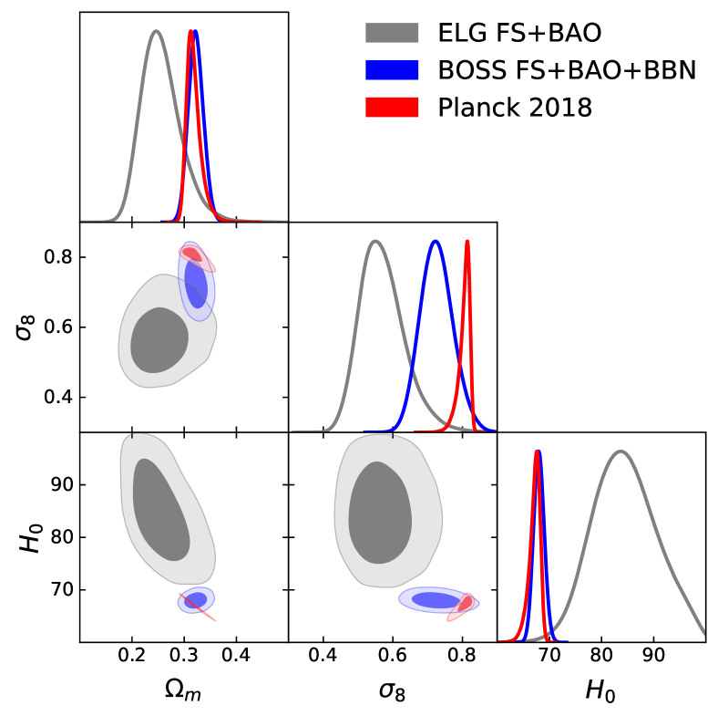
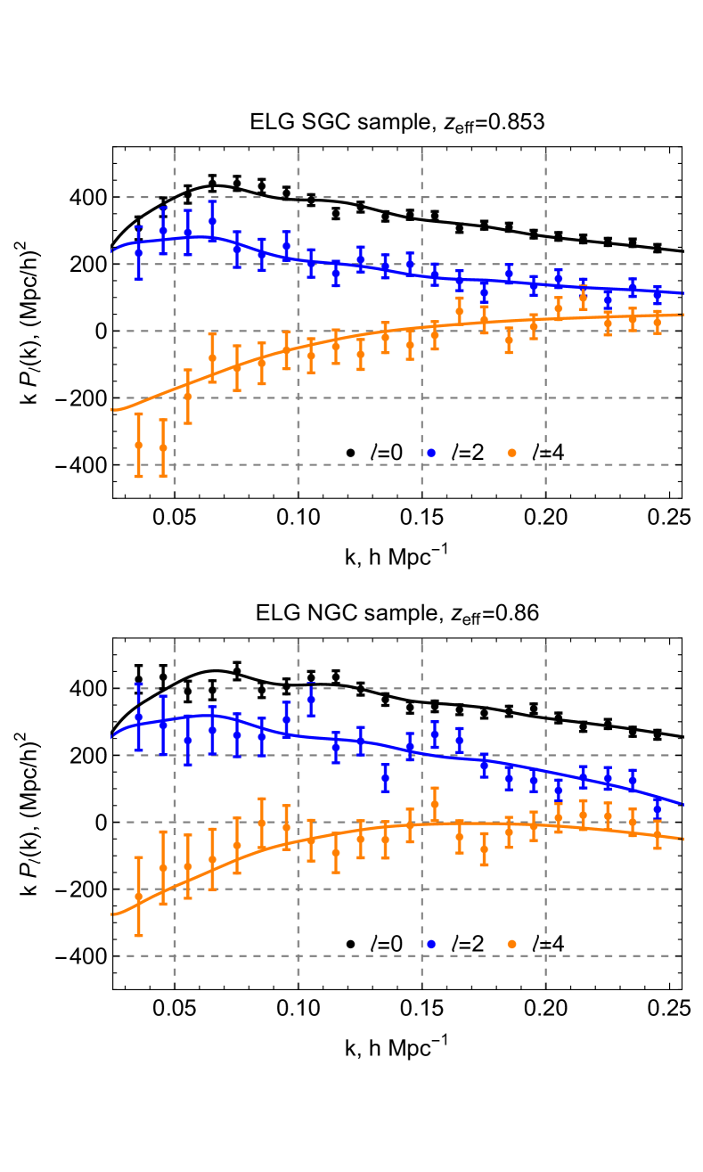
The posterior distribution of the ELG FS+BAO data in planes is shown in the left panel of Fig. 1, along with contours from the combined BOSS FS+BAO+BBN analysis Philcox et al. (2020), and the Planck 2018 data Aghanim et al. (2018) analyses, run for the same baseline CDM model. The right panel of Fig. 1 shows the eBOSS ELG data along with the best-fitting theoretical models extracted from our MCMC chains. The 1d marginalized constraints are listed in table 1.
3 Data and Methodology
3.1 Data
ELG FS + BAO. Our main analysis is based on the power spectrum from the ELG SDSS DR16 clustering catalog Raichoor et al. (2020), see Ref. Raichoor et al. (2017) for selection details. The ELG sample was selected from the DECam Legacy Survey (DECaLS) grz photometry Karim et al. (2020). We use the publicly available baseline power spectrum measurements of Ref. de Mattia et al. (2021). Note that these measurements made use of the so-called “shuffled” scheme where randoms are assigned data redshifts, which suppresses the radial modes on large scales de Mattia and Ruhlmann-Kleider (2019). The eBOSS ELG sample may also be affected by unknown angular systematics, which is mitigated by canceling the angular modes with the so-called pixelated scheme. We refer the reader to Refs. Raichoor et al. (2020); Tamone et al. (2020); de Mattia et al. (2021) for details on the eBOSS ELG catalog and its systematics.
The NGC and SGC patches used in the full-shape analysis have different effective redshifts , number densities , and effective geometric volumes ,
| (1) |
| (2) |
The ELG BAO signal is extracted from the post-reconstructed power spectra measurements in the range . Reconstruction Eisenstein et al. (2007) was performed assuming the logarithmic growth parameter , the linear bias , and using a Gaussian smoothing kernel of width Mpc/.
In our analysis we will use the publicly available pre- and post-reconstructed eBOSS ELG power spectrum multipoles computed from the FKP-weighted density field Feldman et al. (1994) with the Yamamoto estimator Yamamoto et al. (2006) implemented in the nbodykit code Hand et al. (2018). The power spectrum is binned in spherical shells of width . The redshifts and angles are converted into comoving distances assuming a flat CDM cosmology with .
BOSS FS+BAO+BBN. Our additional analyses will be based on the BOSS DR12 LRG full-shape power spectrum data from Alam et al. (2017) combined with the complete SDSS BAO measurements and BBN. We will use the latest version of the EFT-based full-shape LRG power spectrum likelihood described in detail in Refs. Ivanov et al. (2020b); Philcox et al. (2020); Chudaykin et al. (2020); Wadekar et al. (2020). In this work, we will employ the same likelihood as in Ref. Chudaykin et al. (2020), but use the new window-free power spectrum measurements of Ref. Philcox (2021).222Publicly available at https://github.com/oliverphilcox/BOSS-Without-Windows. Our likelihood is based on the monopole, quadrupole, and hexadecapole moments with and . We include the hexadecapole for completeness, even though it contains very little cosmological information for the BOSS LRG sample Chudaykin et al. (2020).
The tail of the BOSS LRG full-shape data has a small overlap with the ELG sample over the redshift rage . This overlap is quite insignificant and we neglect a correlation between the eBOSS ELG and BOSS LRG samples in this work. This assumption was validated in Refs. Alam et al. (2021); Zhao et al. (2021a).
As far as the BAO data is concerned, we use measurements from BOSS DR12 Beutler et al. (2017a), and include their cross-covariance with the full-shape data as described in Ref. Philcox et al. (2020). We compute the cross-covariance between the BAO and full-shape measurements from the Patchy mocks Kitaura et al. (2016). Additionally, we use the BAO from 6DF () Ross et al. (2015), SDSS DR7 MGS () Beutler et al. (2011), and Lyman- forest, which is based on auto and cross-correlation with quasars at du Mas des Bourboux et al. (2020); Alam et al. (2021). Finally, we also use the BAO measurements from the eBOSS quasar sample () Neveux et al. (2020).
We will combine all our large-scale structure likelihoods with the BBN physical baryon density prior , extracted from a conservative standard analysis of data from Aver et al. (2015); Cooke et al. (2018).
Finally, let us briefly comment on the data nomenclature. For brevity we do not mention “BBN” in the ELG FS+BAO likelihood, but it should be recalled that it always contains the BBN prior.
3.2 Theory model
We fit the ELG power spectrum multipoles’ data using the one-loop perturbation theory model described in detail in Refs. Ivanov et al. (2020b); Chudaykin et al. (2020, 2021a, 2021b). The theoretical templates are computed using the CLASS-PT code Chudaykin et al. (2020). In this work we vary all the one-loop power spectrum nuisance parameters in our MCMC chains, including a full set of stochastic counterterms,
| (3) |
Even though some of these contributions cannot be determined by the data itself, and they could be set to constant values (typically zero, see e.g. Ivanov et al. (2020b)), we believe that it is more appropriate to marginalize over all of them within physically motivated priors. These priors will be discussed shortly.
3.3 Window function
Survey geometry. The publicly available eBOSS ELG power spectrum has been obtained using the FKP estimator, which measures the true spectrum convolved with the survey window function. We use the publicly available measurements of the survey window function de Mattia et al. (2021). It is important to mention that the eBOSS ELG window function includes fine-grained veto masks, which make the window function kernels scale-dependent even on small scales (see Fig. 3 or Fig. 1 of Ref. de Mattia et al. (2021)).
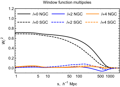
We take the window function effects into account by employing the method of Refs. Wilson et al. (2017); Beutler et al. (2017b) based on the global plane parallel approximation. This method amounts to a simple multiplication of the true position space correlation function multipoles with window function multipoles , i.e. for our analysis involving moments up to the hexadecapole we have
| (4) |
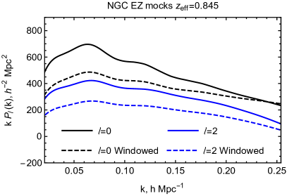
We have checked that higher order window function miltipoles do not affect our results, in agreement with conclusions of Ref. de Mattia et al. (2021). The effect of the window function is illustrated in the upper panel of Fig. 4.
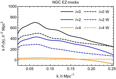
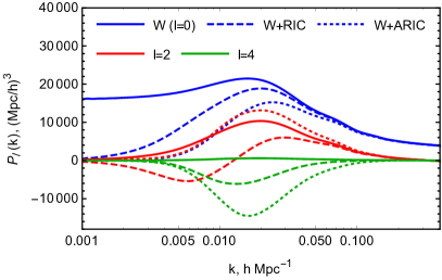
Lower panel: the impact of the integral constraints on the (blue), (red), (green) moments. We show the windowed spectra without integral constraint corrections (“W”, in solid), the effect of the global and radial constrains (“W+RIC”, dashed) and the cumulative effect of the global, angular and radial constrains (“W+ARIC”, dotted), which have to be implemented if the pixelated scheme is used to mitigate the angular systematics.
Integral constraints. We also implement the global, radial and angular integral constraints following Refs. de Mattia and Ruhlmann-Kleider (2019); de Mattia et al. (2021). Schematically, the integral constraint corrected (“icc”) correlation functions have the following form,
| (5) |
where are Legendre multipole moments of the 3-point correlator of the window function de Mattia and Ruhlmann-Kleider (2019). Note that it is crucial to use in Eq. (5) the masked multipoles that contain the full pair count shot noise correction, i.e. Fourier transforms of the full power spectrum with the shot noise term. The effect of integral constraint corrections is illustrated in the lower panel of Fig. 4. One can notice that the radial constraint corrections suppress the quadrupole, while the angular constraint term enhances it. The effect on the monopole is a suppression, which becomes stronger with the angular integral constraint.
Importantly, we see a relatively large effect of the integral constraint on the hexadecapole. The situation here is qualitatively different from the case of the BOSS LRG sample, which is not strongly affected by the integral constraints de Mattia and Ruhlmann-Kleider (2019). Because of this the hexadecapole of the BOSS LRG sample has a relatively weak amplitude and does not improve cosmological constraints. In contrast to that, the eBOSS ELG hexadecapole is dominated by the leakage from the monopole and quadrupole moments through the integral constraints. This results in a relatively strong amplitude of the hexadecapole signal. Because of this effect we may expect that the ELG moment should be important for parameter constraints and therefore we take this moment into account.
Fiber collisions. Finally, we implement the effective window method in order to account for fiber collisions Hahn et al. (2017). This method consists of two steps. First, one corrects the position space correlation function with a steplike kernel proportional to the fraction of collided pairs ,
| (6) |
where s is the pair separation vector, , , z is the unit line-of-sight vector, , is the Legendre polynomial of order , and is the position space top-hat function with the step scale . For eBOSS ELGs we have de Mattia et al. (2021)
| (7) |
The length scale of the fiber collision window is . This is the comoving size that corresponds to the fiber collision angular scale at . After the convolution with the effective window kernel and the consequent Fourier space transform one must marginalize over a set of nuisance parameters that renormalize the Fourier integral. Specifically, one needs to add the following higher derivative stochastic corrections for each multipole Hahn et al. (2017):
| (8) |
and marginalize over new nuisance parameters . If the survey window function were scale-independent on large scales, for the monopole and quadrupole these parameters would exactly coincide with the EFT stochastic counterterms , and that are already marginalized over in our analysis. For the hexadecapole there is a new higher order stochastic counterterm . The parameters (8) that we use in our analysis will be discussed in detail in the next section.
In Fig. 5 we illustrate the impact of the effective window approach to account for fiber collisions. We show pixelated power spectrum multipoles after correcting them as prescribed by Eq. (6). All nuisance parameters are kept fixed during this procedure. The difference between the “usual” and the fiber-collision corrected spectra are well approximated by a constant for the monopole, by a term for the quadrupole, and by a term for the hexadecapole.
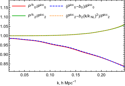
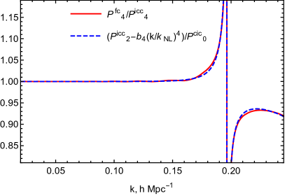
The general approximate formula for the effective window corrections can be written as
| (9) |
where . The best-fitting values for the NGC footprint are given
| (10) |
We see that for the monopole and quadrupole the effective window corrections just renormalize the one-loop EFT nuisance parameters. The hexadecapole fiber collision correction renormalizes the two-loop stochastic counterterm , which is higher order in our nomenclature but we still include it in our model in order to accurately capture fiber collisions.
The degeneracy between the effective window scheme and EFT nuisance parameters was pointed out in Ref. Ivanov et al. (2020b), which argued that marginalization over the stochastic EFT parameters completely captures the effect of fiber collisions even without an explicit implementation of the effective window function corrections. However, including these corrections has no impact on computational time, and we prefer to keep them in our analysis for completeness.
3.4 Parameters and priors
Let us discuss priors on cosmological and nuisance parameters that we impose in our ELG full-shape analysis. These priors are similar to those used in the DES year 3 cosmological analysis Abbott et al. (2021),
| (11) |
As far as the nuisance parameters are concerned, we use the following priors for biased parameters Chudaykin et al. (2020); Wadekar et al. (2020),
| (12) |
higher derivative terms (counterterms)
| (13) |
and stochastic contributions
| (14) |
where we have introduced the notation for a Gaussian distribution of a variable with mean and variance . Note that our convention for the stochastic contributions is given by,
| (15) |
with . The publicly available eBOSS measurements have the windowed Poissonian shot noise contribution subtracted from the data de Mattia et al. (2021). To account to this we subtract the term from the window-convolved monopole templates in our likelihood.
As part of the effective window method to capture fiber collisions, we need to marginalize the windowed theory model over stochastic contributions given in Eq. (8). Because of the scale-dependence of the window function, the fiber-collision induced stochastic terms are not exactly degenerate with the “fundamental” stochastic contribution (15). Hence, we additionally marginalize over the stochastic fiber collision corrections (8). Based on tests with mocks with injected fiber collisions, we found that it is sufficient to use the three new parameters and with the following priors:
| (16) |
Note a few differences in the choice of priors w.r.t. former LRG analyses Chudaykin et al. (2020, 2021b). We double the standard deviations in priors for and , which is motivated by recent simulation-based evidence that these biases deviate from those of host halos for weakly biased galaxies such as ELGs Eggemeier et al. (2021); Barreira et al. (2021). The second point is that we use smaller mean values in priors for fingers-of-God counterterms and , which reflects the fact that the velocity dispersion of ELGs is expected to be somewhat smaller than that of LRGs. The third point is that we use a more conservative model for the stochastic contributions. We explicitly marginalize over the higher derivative stochastic counterterm now and also significantly increase the standard deviation in the prior for the constant shot noise contribution, which is chosen in order to account for a possible super-Poissonian sampling, which can take place for weakly biased tracers such as ELGs Schmittfull et al. (2019, 2019).
Since the SGC and NGC samples have different sky calibrations, we use a separate set of nuisance parameters for each footprint.
3.5 Likelihood
We sample the Gaussian power spectrum likelihood
| (17) |
and . We use the publicly available covariance matrix estimated from 1000 realizations of EZ mocks Zhao et al. (2021b). Our combined FS+BAO analysis will be based on the datavector , where is the isotopic BAO scaling parameter. The covariance of this datavector will be estimated from the same EZ mocks using the method of Ref. Philcox et al. (2020).
4 Tests on simulations
4.1 Outer Rim mocks
We determine the maximal scale cut of our theory model by analyzing Outer Rim ELG mocks. These mocks were designed to match observed properties of the eBOSS ELG sample Avila et al. (2020) and were used to validate the baseline eBOSS analysis pipeline Alam et al. (2020); Rossi et al. (2020). The mocks are generated from the Outer Rim dark matter simulation Heitmann et al. (2019), which has 27 Gpc3 volume and has been run for the following fiducial CDM cosmology:
| (18) |
The simulation snapshot at was populated with mock ELGs using several different halo occupation distribution (HOD) models. In our analysis we focus on the HOD-3 model, which was a default choice of the eBOSS collaboration Avila et al. (2020). Within this model, the large-scale power spectrum primarily depends on the satellite galaxy fraction . This is an important parameter in the EFT context as well, as it controls the strength of the fingers-of-God effect, and hence is linked with the cutoff of the redshift-space mapping expansion Hand et al. (2017); Chudaykin and Ivanov (2019); Ivanov et al. (2020b); Chudaykin et al. (2020). Given this reason, we analyze three sets of HOD-3 mocks that differ by the satellite fraction, . These mocks have large number densities of [Mpc, which is approximately 10 times larger than the number density of the actual ELG sample.
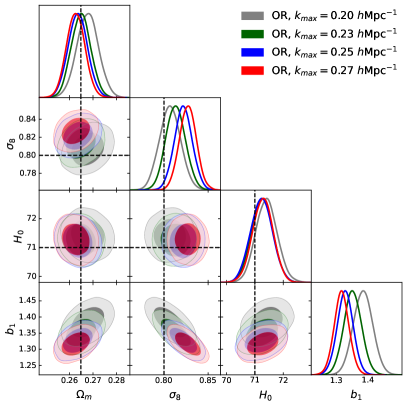
The corresponding mock catalogs are publicly available in the form of 27 non-overlapping subboxes of size 1 Gpc3, which were cut out from the full Outer Rim box. We combine these public subboxes into the original large box with periodic boundary conditions, and compute the mock power spectrum multipoles with the nbodykit code Hand et al. (2018) using a -grid and Triangular-Shape-Cloud mass assignment. We bin the power spectrum in uniform -shells of width , and assume the true fiducial CDM cosmology with in the redshift/angles-to-distance conversion.
For each HOD we fit the mock power spectrum from the total Outer Rim box, which has the volume of Gpc3. Additionally, in order to reduce statistical scatter in the velocity field we average power spectrum multipoles over three independent line-of-sight directions following Ref. Smith et al. (2020b). At this level of precision, we also account for binning and discreteness effects along the lines of Ref. Nishimichi et al. (2020). We employ the Gaussian periodic box boundary condition approximation for the covariance matrix with the effective volume Gpc3. We have computed the covariance both using the analytic linear theory disconnected part expression Wadekar and Scoccimarro (2019) and the empirical estimator for the diagonal elements from sub-boxes. In the latter case we divided the covariance elements by 27 to match the total simulation volume.333The mean from individual subboxes is expected to deviate from the power spectrum computed from the full box at the level of due to super-sample effects de Putter et al. (2012), which is totally negligible for our purposes. This was explicitly checked in Ref. Rossi et al. (2020). The two options give statistically consistent posteriors, and here we present results obtained with the analytic Gaussian covariance. As an additional test, we have repeated our analysis for the covariance that includes the connected non-Gaussian contribution computed in perturbation theory along the lines of Ref. Wadekar and Scoccimarro (2019). In agreement with previous studies Wadekar et al. (2020); Philcox et al. (2021b), we have found the impact of the non-Gaussian covariance elements to be negligibly small.444We thank Jay Wadekar for his help with this analysis.
We have fitted the Outer Rim ELG mock power spectrum multipoles using the full one-loop perturbation theory model of Refs. Ivanov et al. (2020b); Chudaykin et al. (2020, 2021b) with the priors on nuisance parameters specified above. We have fixed , and to their fiducial values and explicitly varied , and in our MCMC chains. Fixing , and is optional. We do so in order to access the accuracy of the other parameter recovery in the situation when they are most tightly constrained. Varying , and in the fit would inflate the posteriors and might obscure the model performance evaluation. We choose to present our main results for and derived parameters and , which we expect to constrain from the actual data and which are more common in the large-scale structure literature.
Strength of fingers-of-God. As a first step, we have verified that the ELG power spectrum requires the next-to-leading order fingers-of-God Jackson (1972) operator just like the LRG sample, but its amplitude is smaller than that of the LRGs (taken e.g. from the analysis of Ref. Nishimichi et al. (2020)555In contrast to the original East Coast Team analysis of Ref. Nishimichi et al. (2020), in order to extract here we fitted the full set of nuisance parameters, including the stochastic counterterms. This is crucial for unbiased estimation of nuisance parameters, which are highly correlated among each other. ):
| (19) |
Here we quote obtained from the analysis of the mocks at . Recalling the relationship between and the cutoff of the redshift-space mapping in the EFT we obtain estimates
| (20) |
Thus, we see that the ELG RSD cutoff is of the same order as the cutoff of the LRG sample. A similar conclusion holds true even for mocks with .
It is also instructive to compare the cutoffs extracted from the quadrupole counterterms () of ELG and LRG samples. We have
| (21) |
which gives the same estimates for the nonlinear scale as in Eq. (20). Note that these counterterms can be interpreted as the short-scale velocity dispersion , implying
| (22) |
All in all, we conclude that the fingers-of-God effect is indeed somewhat weaker for the ELG sample, but it is not sufficiently small to allow us to set even for the vanishing satellite fraction .
Cosmological constraints. As a second step, we fit the mock spectra for seven data cut choices
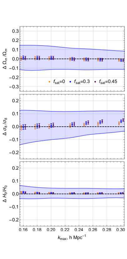
Our results for the 1d marginalized posteriors of and are displayed in Fig. 6. We show the fractional difference between the recovered and the true values, e.g. . The blue band represents the errorbar estimates for the times smaller survey volume, which is roughly equal to the ratio of volumes of the mocks and the actual eBOSS ELG sample. The triangle plot for the parameters measured in the case are shown in Fig. 7, the 1d marginalized posteriors are displayed in Table 2.
Looking at the top of Fig. 6, we see that the true values of and are recovered within (68-95)% CL for all and HOD variants.666The difference w.r.t. the previous version of this paper that had some bias on is due to the subboxes’ treatment. Previously, we averaged spectra from subboxes. However, when measuring these spectra we incorrectly assumed periodicity of the individual subboxes. In contrast, now we combine the subboxes into the original simulation box and then measure the spectrum from the total catalog. This procedure allows us to reconstruct the correct spectrum of the simulation satisfying periodic boundary conditions, thereby removing the bias on . The recovery is unbiased until , after which the measured exhibits a bias growing with . The situation here is similar to the behavior seen in the analyses of large-volume LRG mock data Ivanov et al. (2020b); D’Amico et al. (2019); Nishimichi et al. (2020); Chudaykin et al. (2021a). In the LRG case the recovery is unbiased up to , after which the bias grows and reaches the level of at . It is important to mention that this LRG trend hardly depends on redshift (in the range ), which suggests that it would also hold true at the redshift of our mock ELG sample . We see that the ELG sample is somewhat better because the analysis is unbiased up to , and the bias appears at . Even though this difference is quite insignificant for eBOSS, it may be important for future surveys like DESI/Euclid, for which our results suggest that the EFT analysis indeed may be pushed to smaller scales.
To put this claim in context, let us notice that several forecasts, e.g. Aghamousa et al. (2016); Ivanov et al. (2020c); Sailer et al. (2021) suggest that DESI will probe the velocity fluctuation amplitude with precision if the analysis is carried out at scales . Achieving this goal is feasible with the ELG sample within our analysis, which produces unbiased results at this . Notice also that at this DESI is not affected by observational or instrumental systematics, and not dominated by shot noise Aghamousa et al. (2016). However, if the strength of non-linear RSD were comparable to that of the LRG sample, we would be forced to stop at Nishimichi et al. (2020) by theoretical systematics, so that the precision would degrade by a factor of two, i.e. down to Aghamousa et al. (2016); Nishimichi et al. (2020).
The bias on is somewhat stronger for mocks with larger , in agreement with arguments from the previous literature, see e.g. Chudaykin and Ivanov (2019); Chen et al. (2020). However, we see a similar bias even for mocks without satellites, which suggests that they are not the main culprit of strong fingers-of-God. In the EFT context, the apparent bias on is a signature of two-loop corrections omitted in our theory model. In principle, the two-loop corrections can be partly taken into account by the theoretical error covariance Chudaykin et al. (2021a). However, in terms of the true eBOSS ELG error bars, the bias due to two-loop corrections is quite small. This bias reaches of the true statistical error on from the eBOSS data at . Therefore, we believe that the choice accomplishes a good balance between the statistical and systematic errors.
All in all, we conclude that our theory model should describe the actual ELG data accurately enough up to .
4.2 Reference EZ mocks
| NGC | |||
|---|---|---|---|
| SGC | |||
| SGC+NGC |
In this section we test our pipeline on approximate EZ lightcone mocks. These mocks are based on the Zel’dovich approximation for the gravity solver, but they capture the lightcone effects, survey geometry, veto masks, and other observational features present in the actual data Zhao et al. (2021b). We start by analyzing the reference set of mocks, which include the survey geometry and veto masks, but not the observational systematics. The reference set consists of 1000 catalog realizations mimicking ELG clustering in northern and southern galactic caps in the redshift range . Following de Mattia et al. (2021), we model corresponding spectra as if they were taken at a single snapshot with . The mock fiducial cosmology is given by
| (23) |
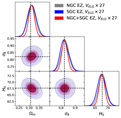
We fit the mean of 1000 mocks with the corresponding empirical sample covariance rescaled by in order to match the volume of the Outer Rim mocks. Since the reference mocks do not contain observational systematics, we do not implement the integral constrains and fiber collision corrections in our theory templates. We restrict our analysis to (following Ref. de Mattia et al. (2021)) and . As in the previous section, we vary the cosmological parameters and in our chains and fix all other cosmological parameters to their fiducial values. In Fig. 8 and table 3 we show results of our analysis for SGC and NGC chunks separately and their combination. For clarity we show only the parameters and . The first important observation is that our pipeline recovers true values of cosmological parameters without any noticeable bias. The second observation is that the precision of cosmological parameter measurements from the EZ mocks is noticeably worse than those from the OR mocks without the survey window function, especially for and .
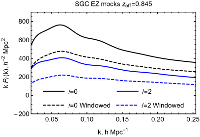
In the next section we will see the actual ELG full-shape data alone cannot strongly constrain the Hubble parameter. This happens because of several reasons. First, the effective volume of this sample, is relatively small. Second, this sample has a specific shape of the window function, which is noticeably suppressed for pair separations Mpc. This suppression translates into a suppression of the BAO feature, which is crucial for the measurement from the full shape Ivanov et al. (2020b). Because of these effects, previous analyses were not able to confidently detect the BAO feature in ELG sample even after applying the reconstruction technique de Mattia et al. (2021). The suppression effect can be observed in Fig. 9, which displays a typical ELG power spectra from our MCMC chains before and after the convolution with the window function. We see that the unwindowed power spectrum monopole exhibits a clear BAO signature, which becomes suppressed after the window function application. As far as the quadrupole moment is concerned, we do not expect to have a strong BAO feature without reconstruction. The BAO in the quadrupole is suppressed due to IR resummation to begin with Ivanov and Sibiryakov (2018), and the relatively high shot noise level of the eBOSS ELG sample makes it unlikely that the residual BAO signature could be detected even if the effects of the window function were completely absent.
4.3 Contaminated EZ mocks
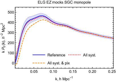
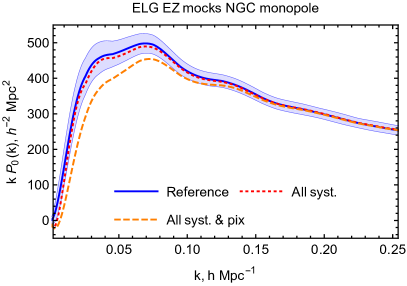
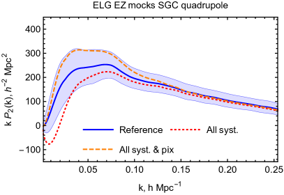
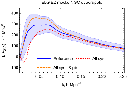
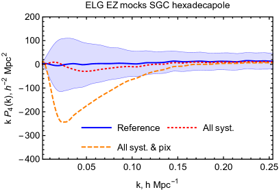
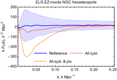
In order to test the perfomance of our pipeline on actual observations, we analyze now the “contaminated” EZ mocks with injected systematic effects. The dominant effects are angular photometric uncertainties, shuffling that is used to generate random catalogs, and fiber collisions. In order to mitigate the angular systematics, the correction (“pixelation”) scheme is used, which introduces new alternations to the power spectrum shape. The cumulative systematic effect with and without pixelation, as modelled in the mocks, can be seen in Fig. 10. There we display the power spectrum multipoles of the contaminated mock catalogs, along with their pixelated version, and the reference mocks discussed before. Note that both contaminated and pixelated mocks correspond to slightly different redshift interval , which is chosen in order to exclude data with large variations of the redshift density with photometric depth present in the range . The effective redshift of the contaminated mocks is .
We can see that the contaminated mocks exhibit a clear suppression in the quadrupole, and this suppression can be partly taken into account means of the radial integral constraint. In contrast, after applying the pixelation scheme, the quadrupole becomes enhanced. This enhancement can be taken into account by means of the radial and angular integral constraints. In order to illustrate that, in Fig. 11 we overplot the fiducial theory templates curves on top of curves from Fig. 10. To obtain the theory predictions we took the best-fit parameters of the reference mocks (“Ref. bf”) and applied global+radial integral constraint to model the unpixelated data (“Ref. bf + RIC”) and the global+radial+angular integral constraint to model the pixelated measurements (“Ref. bf + ARIC”). We see that in the unpixelated case (“All syst”) the agreement between the model and the mocks is not perfect for the quadrupole and hexadecapole on large scales . This is a result of unaccounted for angular systematics. Once the angular systematics is mitigated by means of the pixelated scheme, the agreement between the mocks and the theory model becomes restored essentially on all scales.
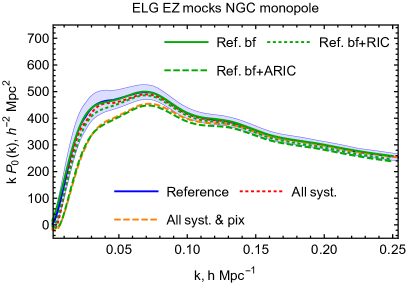
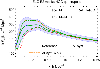
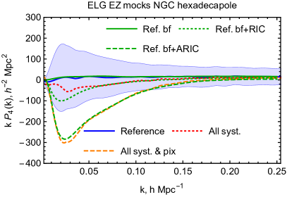
If not accounted for, the scale-dependent modulation of the power spectrum due to radial and angular systematics would be a very strong source of systematics in our full-shape analysis. As an example, in Fig. 12 and table 4 we present the results of the analysis of the pixelated spectra without implementing integral constraint corrections (“all syst. & pix, no corr.”). We see that and are strongly biased in that case. As a second test, we present the analysis of the non-pixelated spectra with all systematics injected and with full modeling including the integral constraints and fiber collisions (“all syst. & nopix, corr.”). We see that parameter recovery is satisfactory in this case, but the unaccounted for angular systematics leads to a bias on . This bias originates due to the additional suppression of the quadrupole on large scales clearly seen in Fig. 11. As anticipated, cosmological parameter recovery is unbiased after implementing the pixelated scheme, which is accurately modeled by means of the angular integral constraint, see “all syst. & pix, corr.” in Fig. 12.
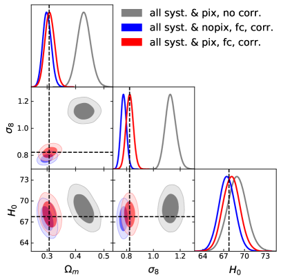
| pix, no corr. | |||
|---|---|---|---|
| nopix, fc, corr. | |||
| pix, fc, corr. |
4.4 Post-reconstructed BAO data
Now let us discuss the post-reconstructed power spectra, which we analyze using the method proposed in Philcox et al. (2020). We have found that the eBOSS ELG data cannot constrain the anisotropic BAO signal, and hence we focus only on the isotropic part, which is extracted from the post-reconstructed monopole power spectrum moment. The angle-averaged BAO signal is encapsulated by a parameter ,
| (24) |
where we introduced the effective spherically averaged comoving distance
| (25) |
is the comoving angular diameter distance, is the Hubble parameter, is the comoving sound horizon at the drag epoch, and “fid.” refers to quantities computed in reference cosmology used to generate the fixed power spectrum template. We choose the same fiducial cosmology as Ref. de Mattia et al. (2021). We stress here that unlike the full-shape measurements, the use of a fixed template is accurate in the BAO context. Our post-reconstructed power spectrum model is the same as in Ref. Philcox et al. (2020). We account for non-linear effects on the broadband part by means of the theoretical error approach Baldauf et al. (2016c); Chudaykin et al. (2021a), which provides an efficient way to marginalize over the shape uncertainties.
As a first step, we measure the isotropic BAO signal from 1000 contaminated SGC EZ mocks. We use the mocks that span the full redshift range , because the photometric systematics discussed above does not bias the BAO signal recovery. For each mock we fit the parameters (post-reconstructed BAO smearing scale), and . The latter is constrained to a prior range de Mattia et al. (2021). The binned histogram of extracted best-fit values of are shown in Fig. 13. Apparent enhancements at the prior boundaries correspond to mocks where the BAO feature is not detected. The robust BAO detection can be characterized by requirements that the best-fit lies within confidence interval and this interval does not touch the prior boundaries,
| (26) |
where is the upper/lower boundary of the 68% confidence interval computed using the two-tailed method.
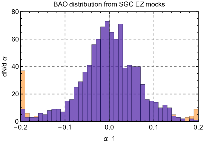
Overall, we have not detected the BAO in 46 mocks out of 1000. We discard them in the further analysis. The mean value of from the remaining set matches the true value to accuracy,
| (27) |
The rms standard deviation from the “good” mocks is . Using the best-fit value of from each SGC mock we compute the covariance between the pre-reconstructed SGC spectra and with the usual empirical estimator. We have also repeated the same analysis for the NGC chunk, but unfortunately we were not able to detect the BAO feature in the actual NGC data. This was also the case in the official eBOSS ELG analysis de Mattia et al. (2021). Therefore, for this footprint we proceed with the pre-reconstructed data only.
4.5 Joint FS+BAO analysis
Now we jointly fit the full-shape and BAO EZ mock data using the same pipeline and similar analysis choices as in the actual data analysis. We will vary now all relevant cosmological parameters assuming the priors (11). As before, we will fit the mean of mocks and rescale the covariance by a factor 27. As a first step we analyze the full-shape ELG data with . As a second step we add the BAO data and fit the joint ELG FS+BAO likelihood. As before, we use the FS-BAO EZ mock data covariance rescaled by 27 and fit the mean of the BAO parameter extracted from SGC EZ mocks. For the NGC part we use only the full-shape measurements.
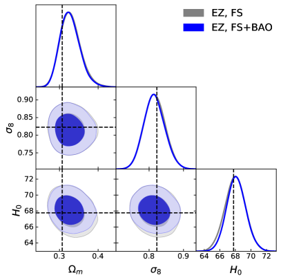
| FS | |||
|---|---|---|---|
| FS+BAO |
Our results are presented in Fig. 14 and Table 5. We observe that the contours have more non-Gaussian shape now because of correlations between the measured parameters and parameters that are determined by priors. This also explains some apparent shifts in the posteriors, which are driven by prior volume effects. In particular, is shifted down w.r.t. the reference analysis in table 3 because of marginalization over the neutrino mass. Finally, we see that the addition of the post-reconstructed BAO data improves the parameter constraints only marginally. In particular, the posterior for sharpens only by .
5 Results
ELG full-shape data alone. Let us start with the baseline analysis of the ELG FS data alone. We jointly fit the SGC+NGC monopole, quadrupole and hexadecapole power spectra with (following the analysis of Ref. de Mattia et al. (2021)) and for three choices of , and .
In all analyses, we have found that the posterior is not sufficiently narrower than the prior. Hence, we do not present its measurements. As we have explained before, this happens because of a relatively small effective volume and a particular shape of the ELG window function.
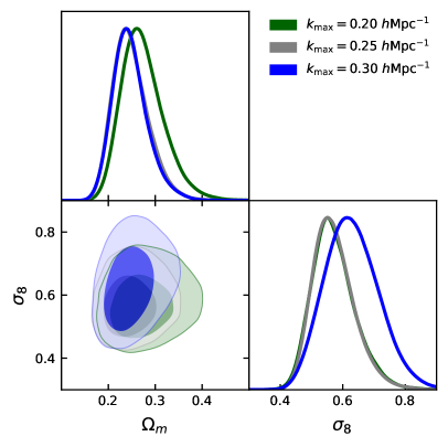
Due to a limited effective volume, we cannot significantly constrain other parameters like and . Because of this, we present the results for and only. The posteriors for the three different data cuts are shown in Fig. 15 and in table 6. The posterior is significantly non-Gaussian. We see that results at and are very consistent with one another, with the contours being somewhat narrower in the latter case. However, the 1d marginalized posterior shifts upward by 1 when is increased up to . This shift is very similar to the typical biases induced by two-loop corrections that we have seen in the simulation data analysis. Another interesting feature is the increase of the 1d marginalized error on at . This may indicate residual systematics in the data or be an artifact of the one-loop EFT, which is expected to break down at these scales. All in all, we select as our baseline.
As an additional test, we repeat our baseline analysis without the fiber collision corrections, see table 6. In this case we find almost identical optimal values of relevant cosmological parameters. The only noticeable effect is that the variance of is underestimated by if the fiber collision corrections are completely ignored.
Addition of the ELG BAO data. Applying our BAO analysis pipeline to the SGC data we have obtained the following measurement of the isotropic BAO parameter,
| (28) |
where in the parenthesis we quote the best-fit value. As an additional test, we fix as in Ref. de Mattia and Ruhlmann-Kleider (2019) and obtain essentially the same result,
| (29) |
| FS () | CL) | ||
|---|---|---|---|
| FS () | CL) | ||
| FS () | CL) | ||
| FS (), no fc | CL) | ||
| FS ()+BAO |
The NGC chunk does not carry any detectable BAO signal de Mattia et al. (2021). Now we perform a joint ELG FS+BAO fit, whose results are summarized in Table 6 and in Fig. 1. The addition of the BAO allows us to measure the Hubble constant, although with large errors. Indeed, unlike the case of the FS data alone, the confidence limit on from the ELG FS+BAO analysis is within the prior, km/s/Mpc (95% CL).
To put our measurements in context, in Fig. 1 we plot our posteriors along with the CMB Planck 2018 and FS+BAO+BBN measurements for the same parameters. Overall, we observe a satisfactory agreement between the FS+BAO measurements from BOSS and eBOSS ELG. At face value, the agreement with Planck is worse, but the interpretation here is complicated by the fact that ELG contours are significantly non-Gaussian. In particular, the posterior exhibits a massive tail towards large values. Regardless of this issue, the ELG posterior overlaps with the Planck one within 99CL, which is still consistent with a hypothesis that both data vectors are drawn from the same parameter set.
Comparison with previous work. Let us compare our results with the official ELG BOSS analysis from Ref. de Mattia et al. (2021). Note that the RSD/AP parameters , and are777The latter are defined as , ( is the speed of light) . derived parameters in our FS+BAO analysis, and also they are subject to the CDM model priors. The values extracted from our MCMC chains read:
| (30) |
Our measurements agree within confidence intervals with the baseline RSD/AP measurements from the eBOSS ELG power spectrum reported in Ref. de Mattia et al. (2021):
| (31) |
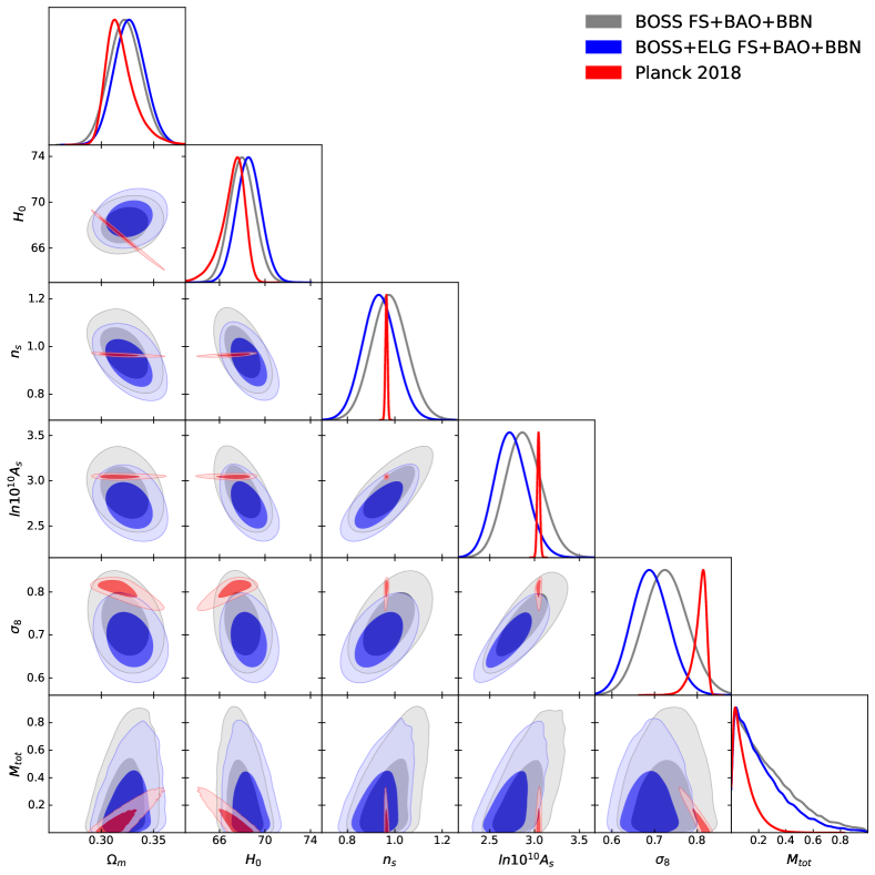
Joint analysis of ELG and LRG FS and BAO data. Given a satisfactory agreement between the BOSS FS+BAO+BBN dataset and the ELG FS+BAO data in the plains, we can combine them. The joint BOSS FS+BAO+BBN + ELG FS+BAO likelihood provides reasonable constraints on all cosmological parameters, including the neutrino mass and the spectral index. The results for this analysis, along with the Planck CMB contours for the same CDM model are displayed in Fig. 2. We see that the addition of the ELG data slightly tightens the LSS parameter constraints. The maximal improvement can be seen in the plane.
A standard output of RSD measurements is the value of the rms velocity fluctuations at effective redshifts of given samples. These are derived parameters in our joint analysis, which are given by
| (32) |
Using the following tension metric between two measurements Nunes and Vagnozzi (2021),
| (33) |
we estimate that our growth rates from BOSS and eBOSS are in tension with the Planck 2018 results for the same CDM model888https://wiki.cosmos.esa.int/planck-legacy-archive/images/b/be/Baseline_params_table_2018_68pc.pdf , , .
In order to check whether this conclusion is sensitive to Bayesian marginalization effect, we do the following test. First, we analyze the BOSS+ELG FS+BAO data fixing all cosmological parameters to the Planck 2018 (P18) baseline best-fit values. All nuisance parameters are allowed to vary. The total neutrino mass is fixed to it minimal value eV. Second, we repeat the same analysis but additionally vary the primordial spectral amplitude in our MCMC chains. We find the constraints,
| (34) |
The effective difference between these two cases is
| (35) |
which corresponds to a tension. We conclude that the tension is present even from the frequentest point of view but the impact of Bayesian volume effects is not negligible; it accounts for about of the “Bayesian” tension.
Another cosmological parameter important in the context of the weak lensing measurements is , whose value from our MCMC chains is given by
| (36) |
This value is broadly consistent with the DES year 3 weak lensing measurement Abbott et al. (2021) ( in this case), but it is still in some tension with the Planck CMB Aghanim et al. (2018) , .
On the one hand, our analysis confirms the trend of lower structure clustering observed in other large-scale structure datasets, known as “ tension,” see Ref. Di Valentino et al. (2021) for a recent review. On the other hand, the statistical significance is still not very significant, which suggests that this “tension” can still be treated as a statistical fluctuation. Systematic errors in the RSD measurements, such as the contamination by selection bias Hirata (2009); Obuljen et al. (2020), are also not excluded.
Bias parameters. The posteriors for nuisance parameters are not significantly narrower than the priors, except for the linear bias. The values extracted from the most constraining joint FS+BAO+BBN analysis yield
| (37) |
which are broadly consistent with expected values for the ELGs. For completeness, we present measurements of nuisance parameters, even though their posteriors are mostly determined by the priors (see Appendix A for the full table including the BOSS samples),
| (38) |
6 Discussion
In this work we have carried out a full-shape analysis of the eBOSS emission line galaxy sample. Our main results are:
-
•
We determined the data cut for the one-loop EFT description of the ELG power spectrum at to be , depending on the target theoretical error tolerance.
-
•
The ELG power spectrum model requires the next-to-leading order finger-of-God operator just like the power spectrum of LRGs. However, the momentum cutoff scale of this operator is higher for ELGs than that of LRGs, and hence the EFT analysis could be pushed to somewhat smaller scales.
-
•
The current eBOSS ELG power spectrum and BAO data alone constrain , , and . These results are in a tension with the Planck CDM model, but this discrepancy is not statistically significant. Our measurements are broadly consistent with other CMB and large-scale structure datasets.
Forecasts of Refs. Chudaykin and Ivanov (2019); Sailer et al. (2021) suggest that the full-shape analysis of power spectra from Euclid/DESI-like surveys will be able to strongly constrain our Universe’s parameters and detect neutrino masses. These surveys will mainly target emission line galaxies, whose observational properties are not fully understood. In this work we have started exploring these galaxies in the context of the full-shape analysis using the largest to date eBOSS catalog. We believe that our analysis will initiate a systematic study of the ELG clustering statistics within the effective field theory framework, which will be important for cosmological parameter measurements from future spectroscopic surveys like DESI and Euclid.
Acknowledgments
We are grateful to Giovanni Cabass, Arnaud de Mattia, Oliver Philcox, Marko Simonović, Martin White and Matias Zaldarriaga for valuable comments on the draft. We thank Jay Wadekar for his help with the non-Gaussian covariance calculation. We also thank Santiago Avila for his help with the Outer Rim mocks. We thank Arnaud de Mattia for sharing with us the eBOSS ELG EZ mock measurements.
Parameter estimates presented in this paper have been obtained with the CLASS-PT
Boltzmann code Chudaykin et al. (2020)999https://github.com/Michalychforever/CLASS-PT,
https://github.com/Michalychforever/lss_montepython.
(see also Blas et al. (2011)) interfaced with the Montepython MCMC sampler Audren et al. (2013); Brinckmann and Lesgourgues (2019)101010https://github.com/brinckmann/montepython_public.
.
The triangle plots are generated with the getdist package111111
https://getdist.readthedocs.io/en/latest/
Lewis (2019),
which is part of the CosmoMC code Lewis and Bridle (2002); Lewis (2013).
Appendix A Constraints table
| Param | best-fit | mean | 95% lower | 95% upper |
|---|---|---|---|---|
| Param | best-fit | mean | 95% lower | 95% upper |
|---|---|---|---|---|
In this appendix we present the full parameter constraints tables 7, 8 from our ELG FS+BAO and BOSS+ELG FS+BAO+BBN analyses. We use the following convention for the upper indices of bias parameters:
| (39) |
The other nuisance parameters are marginalyzed over in our likelihood by means of the exact analytic marginalization.
References
- Peebles (1980) P. J. E. Peebles, The large-scale structure of the universe (1980).
- Percival et al. (2001) W. J. Percival et al. (2dFGRS), Mon. Not. Roy. Astron. Soc. 327, 1297 (2001), arXiv:astro-ph/0105252 .
- Aghanim et al. (2018) N. Aghanim et al. (Planck), (2018), arXiv:1807.06209 [astro-ph.CO] .
- Aiola et al. (2020) S. Aiola et al. (ACT), JCAP 12, 047 (2020), arXiv:2007.07288 [astro-ph.CO] .
- Aylor et al. (2017) K. Aylor et al. (SPT), Astrophys. J. 850, 101 (2017), arXiv:1706.10286 [astro-ph.CO] .
- Bianchini et al. (2020) F. Bianchini et al. (SPT), Astrophys. J. 888, 119 (2020), arXiv:1910.07157 [astro-ph.CO] .
- Asgari et al. (2021) M. Asgari et al. (KiDS), Astron. Astrophys. 645, A104 (2021), arXiv:2007.15633 [astro-ph.CO] .
- Abbott et al. (2018) T. M. C. Abbott et al. (DES), Phys. Rev. D98, 043526 (2018), arXiv:1708.01530 [astro-ph.CO] .
- Abbott et al. (2021) T. M. C. Abbott et al. (DES), (2021), arXiv:2105.13549 [astro-ph.CO] .
- Alam et al. (2017) S. Alam et al. (BOSS), Mon. Not. Roy. Astron. Soc. 470, 2617 (2017), arXiv:1607.03155 [astro-ph.CO] .
- Alam et al. (2021) S. Alam et al. (eBOSS), Phys. Rev. D 103, 083533 (2021), arXiv:2007.08991 [astro-ph.CO] .
- Tegmark et al. (2002) M. Tegmark et al. (SDSS), Astrophys. J. 571, 191 (2002), arXiv:astro-ph/0107418 .
- Tegmark et al. (2004) M. Tegmark et al. (SDSS), Astrophys. J. 606, 702 (2004), arXiv:astro-ph/0310725 .
- Cole et al. (2005) S. Cole et al. (2dFGRS), Mon. Not. Roy. Astron. Soc. 362, 505 (2005), arXiv:astro-ph/0501174 .
- Percival et al. (2007a) W. J. Percival et al., Astrophys. J. 657, 645 (2007a), arXiv:astro-ph/0608636 .
- Smith et al. (2003) R. E. Smith, J. A. Peacock, A. Jenkins, S. D. M. White, C. S. Frenk, F. R. Pearce, P. A. Thomas, G. Efstathiou, and H. M. P. Couchmann (VIRGO Consortium), Mon. Not. Roy. Astron. Soc. 341, 1311 (2003), arXiv:astro-ph/0207664 .
- Percival et al. (2007b) W. J. Percival, S. Cole, D. J. Eisenstein, R. C. Nichol, J. A. Peacock, A. C. Pope, and A. S. Szalay, Mon. Not. Roy. Astron. Soc. 381, 1053 (2007b), arXiv:0705.3323 [astro-ph] .
- Alcock and Paczynski (1979) C. Alcock and B. Paczynski, Nature 281, 358 (1979).
- Cabre and Gaztanaga (2009) A. Cabre and E. Gaztanaga, Mon. Not. Roy. Astron. Soc. 393, 1183 (2009), arXiv:0807.2460 [astro-ph] .
- Blake et al. (2011) C. Blake et al., Mon. Not. Roy. Astron. Soc. 418, 1725 (2011), arXiv:1108.2637 [astro-ph.CO] .
- Samushia et al. (2012) L. Samushia, W. J. Percival, and A. Raccanelli, Mon. Not. Roy. Astron. Soc. 420, 2102 (2012), arXiv:1102.1014 [astro-ph.CO] .
- Chuang and Wang (2012) C.-H. Chuang and Y. Wang, Mon. Not. Roy. Astron. Soc. 426, 226 (2012), arXiv:1102.2251 [astro-ph.CO] .
- de Mattia et al. (2021) A. de Mattia et al., Mon. Not. Roy. Astron. Soc. 501, 5616 (2021), arXiv:2007.09008 [astro-ph.CO] .
- Smith et al. (2020a) A. Smith et al., Mon. Not. Roy. Astron. Soc. 499, 269 (2020a), arXiv:2007.09003 [astro-ph.CO] .
- Aghamousa et al. (2016) A. Aghamousa et al. (DESI), (2016), arXiv:1611.00036 [astro-ph.IM] .
- Laureijs et al. (2011) R. Laureijs et al. (EUCLID), (2011), arXiv:1110.3193 [astro-ph.CO] .
- Lesgourgues and Pastor (2006) J. Lesgourgues and S. Pastor, Phys. Rept. 429, 307 (2006), arXiv:astro-ph/0603494 [astro-ph] .
- Poulin et al. (2019) V. Poulin, T. L. Smith, T. Karwal, and M. Kamionkowski, Phys. Rev. Lett. 122, 221301 (2019), arXiv:1811.04083 [astro-ph.CO] .
- Hill et al. (2020) J. C. Hill, E. McDonough, M. W. Toomey, and S. Alexander, Phys. Rev. D 102, 043507 (2020), arXiv:2003.07355 [astro-ph.CO] .
- Ivanov et al. (2020a) M. M. Ivanov, E. McDonough, J. C. Hill, M. Simonović, M. W. Toomey, S. Alexander, and M. Zaldarriaga, Phys. Rev. D 102, 103502 (2020a), arXiv:2006.11235 [astro-ph.CO] .
- D’Amico et al. (2020a) G. D’Amico, L. Senatore, P. Zhang, and H. Zheng, (2020a), arXiv:2006.12420 [astro-ph.CO] .
- Baumann et al. (2012) D. Baumann, A. Nicolis, L. Senatore, and M. Zaldarriaga, JCAP 1207, 051 (2012), arXiv:1004.2488 [astro-ph.CO] .
- Carrasco et al. (2012) J. J. M. Carrasco, M. P. Hertzberg, and L. Senatore, JHEP 09, 082 (2012), arXiv:1206.2926 [astro-ph.CO] .
- Porto et al. (2014) R. A. Porto, L. Senatore, and M. Zaldarriaga, JCAP 1405, 022 (2014), arXiv:1311.2168 [astro-ph.CO] .
- Vlah et al. (2015) Z. Vlah, M. White, and A. Aviles, JCAP 09, 014 (2015), arXiv:1506.05264 [astro-ph.CO] .
- Blas et al. (2016a) D. Blas, M. Garny, M. M. Ivanov, and S. Sibiryakov, JCAP 1607, 052 (2016a), arXiv:1512.05807 [astro-ph.CO] .
- Chen et al. (2021) S.-F. Chen, Z. Vlah, E. Castorina, and M. White, JCAP 03, 100 (2021), arXiv:2012.04636 [astro-ph.CO] .
- Carrasco et al. (2014a) J. J. M. Carrasco, S. Foreman, D. Green, and L. Senatore, JCAP 07, 056 (2014a), arXiv:1304.4946 [astro-ph.CO] .
- Carrasco et al. (2014b) J. J. M. Carrasco, S. Foreman, D. Green, and L. Senatore, JCAP 07, 057 (2014b), arXiv:1310.0464 [astro-ph.CO] .
- Foreman et al. (2016) S. Foreman, H. Perrier, and L. Senatore, JCAP 05, 027 (2016), arXiv:1507.05326 [astro-ph.CO] .
- Baldauf et al. (2015a) T. Baldauf, L. Mercolli, and M. Zaldarriaga, Phys. Rev. D92, 123007 (2015a), arXiv:1507.02256 [astro-ph.CO] .
- Baldauf et al. (2016a) T. Baldauf, E. Schaan, and M. Zaldarriaga, JCAP 03, 007 (2016a), arXiv:1507.02255 [astro-ph.CO] .
- Baldauf et al. (2016b) T. Baldauf, E. Schaan, and M. Zaldarriaga, JCAP 03, 017 (2016b), arXiv:1505.07098 [astro-ph.CO] .
- Konstandin et al. (2019) T. Konstandin, R. A. Porto, and H. Rubira, JCAP 11, 027 (2019), arXiv:1906.00997 [astro-ph.CO] .
- Senatore (2015) L. Senatore, JCAP 1511, 007 (2015), arXiv:1406.7843 [astro-ph.CO] .
- Angulo et al. (2015) R. Angulo, M. Fasiello, L. Senatore, and Z. Vlah, JCAP 1509, 029 (2015), arXiv:1503.08826 [astro-ph.CO] .
- Mirbabayi et al. (2015) M. Mirbabayi, F. Schmidt, and M. Zaldarriaga, JCAP 1507, 030 (2015), arXiv:1412.5169 [astro-ph.CO] .
- Assassi et al. (2014) V. Assassi, D. Baumann, D. Green, and M. Zaldarriaga, JCAP 1408, 056 (2014), arXiv:1402.5916 [astro-ph.CO] .
- Desjacques et al. (2018) V. Desjacques, D. Jeong, and F. Schmidt, Phys. Rept. 733, 1 (2018), arXiv:1611.09787 [astro-ph.CO] .
- Senatore and Zaldarriaga (2014) L. Senatore and M. Zaldarriaga, (2014), arXiv:1409.1225 [astro-ph.CO] .
- Lewandowski et al. (2018) M. Lewandowski, L. Senatore, F. Prada, C. Zhao, and C.-H. Chuang, Phys. Rev. D 97, 063526 (2018), arXiv:1512.06831 [astro-ph.CO] .
- Perko et al. (2016) A. Perko, L. Senatore, E. Jennings, and R. H. Wechsler, (2016), arXiv:1610.09321 [astro-ph.CO] .
- Ivanov and Sibiryakov (2018) M. M. Ivanov and S. Sibiryakov, JCAP 1807, 053 (2018), arXiv:1804.05080 [astro-ph.CO] .
- Vlah and White (2019) Z. Vlah and M. White, JCAP 1903, 007 (2019), arXiv:1812.02775 [astro-ph.CO] .
- Lewandowski et al. (2015) M. Lewandowski, A. Perko, and L. Senatore, JCAP 1505, 019 (2015), arXiv:1412.5049 [astro-ph.CO] .
- Senatore and Zaldarriaga (2017) L. Senatore and M. Zaldarriaga, (2017), arXiv:1707.04698 [astro-ph.CO] .
- Senatore and Zaldarriaga (2015) L. Senatore and M. Zaldarriaga, JCAP 1502, 013 (2015), arXiv:1404.5954 [astro-ph.CO] .
- Vlah et al. (2016) Z. Vlah, U. Seljak, M. Y. Chu, and Y. Feng, JCAP 1603, 057 (2016), arXiv:1509.02120 [astro-ph.CO] .
- Blas et al. (2016b) D. Blas, M. Garny, M. M. Ivanov, and S. Sibiryakov, JCAP 1607, 028 (2016b), arXiv:1605.02149 [astro-ph.CO] .
- Senatore and Trevisan (2018) L. Senatore and G. Trevisan, JCAP 1805, 019 (2018), arXiv:1710.02178 [astro-ph.CO] .
- Baldauf et al. (2015b) T. Baldauf, M. Mirbabayi, M. Simonović, and M. Zaldarriaga, Phys. Rev. D92, 043514 (2015b), arXiv:1504.04366 [astro-ph.CO] .
- Baldauf et al. (2016c) T. Baldauf, M. Mirbabayi, M. Simonović, and M. Zaldarriaga, (2016c), arXiv:1602.00674 [astro-ph.CO] .
- Chudaykin et al. (2021a) A. Chudaykin, M. M. Ivanov, and M. Simonović, Phys. Rev. D 103, 043525 (2021a), arXiv:2009.10724 [astro-ph.CO] .
- Ivanov et al. (2020b) M. M. Ivanov, M. Simonović, and M. Zaldarriaga, JCAP 05, 042 (2020b), arXiv:1909.05277 [astro-ph.CO] .
- D’Amico et al. (2019) G. D’Amico, J. Gleyzes, N. Kokron, D. Markovic, L. Senatore, P. Zhang, F. Beutler, and H. Gil-Marín, (2019), arXiv:1909.05271 [astro-ph.CO] .
- Philcox et al. (2020) O. H. E. Philcox, M. M. Ivanov, M. Simonović, and M. Zaldarriaga, JCAP 05, 032 (2020), arXiv:2002.04035 [astro-ph.CO] .
- Philcox et al. (2021a) O. H. E. Philcox, B. D. Sherwin, G. S. Farren, and E. J. Baxter, Phys. Rev. D 103, 023538 (2021a), arXiv:2008.08084 [astro-ph.CO] .
- D’Amico et al. (2021) G. D’Amico, L. Senatore, and P. Zhang, JCAP 01, 006 (2021), arXiv:2003.07956 [astro-ph.CO] .
- D’Amico et al. (2020b) G. D’Amico, Y. Donath, L. Senatore, and P. Zhang, (2020b), arXiv:2012.07554 [astro-ph.CO] .
- Chudaykin et al. (2021b) A. Chudaykin, K. Dolgikh, and M. M. Ivanov, Phys. Rev. D 103, 023507 (2021b), arXiv:2009.10106 [astro-ph.CO] .
- Laguë et al. (2021) A. Laguë, J. R. Bond, R. Hložek, K. K. Rogers, D. J. E. Marsh, and D. Grin, (2021), arXiv:2104.07802 [astro-ph.CO] .
- Ivanov et al. (2020c) M. M. Ivanov, M. Simonović, and M. Zaldarriaga, Phys. Rev. D 101, 083504 (2020c), arXiv:1912.08208 [astro-ph.CO] .
- Chudaykin and Ivanov (2019) A. Chudaykin and M. M. Ivanov, JCAP 11, 034 (2019), arXiv:1907.06666 [astro-ph.CO] .
- Sailer et al. (2021) N. Sailer, E. Castorina, S. Ferraro, and M. White, (2021), arXiv:2106.09713 [astro-ph.CO] .
- Avila et al. (2020) S. Avila et al., Mon. Not. Roy. Astron. Soc. 499, 5486 (2020), arXiv:2007.09012 [astro-ph.CO] .
- Orsi et al. (2010) A. Orsi, C. M. Baugh, C. G. Lacey, A. Cimatti, Y. Wang, and G. Zamorani, Mon. Not. Roy. Astron. Soc. 405, 1006 (2010), arXiv:0911.0669 [astro-ph.CO] .
- Okumura et al. (2016) T. Okumura et al., Publ. Astron. Soc. Jap. 68, 38 (2016), arXiv:1511.08083 [astro-ph.CO] .
- Orsi and Angulo (2018) A. A. Orsi and R. E. Angulo, Mon. Not. Roy. Astron. Soc. 475, 2530 (2018), arXiv:1708.00956 [astro-ph.CO] .
- Ross et al. (2020) A. J. Ross et al., Mon. Not. Roy. Astron. Soc. 498, 2354 (2020), arXiv:2007.09000 [astro-ph.CO] .
- Raichoor et al. (2020) A. Raichoor et al., Mon. Not. Roy. Astron. Soc. 500, 3254 (2020), arXiv:2007.09007 [astro-ph.CO] .
- Raichoor et al. (2017) A. Raichoor et al., Mon. Not. Roy. Astron. Soc. 471, 3955 (2017), arXiv:1704.00338 [astro-ph.CO] .
- Karim et al. (2020) T. Karim, J. H. Lee, D. J. Eisenstein, E. Burtin, J. Moustakas, A. Raichoor, and C. Yèche, Mon. Not. Roy. Astron. Soc. 497, 4587 (2020), arXiv:2007.14484 [astro-ph.GA] .
- de Mattia and Ruhlmann-Kleider (2019) A. de Mattia and V. Ruhlmann-Kleider, JCAP 08, 036 (2019), arXiv:1904.08851 [astro-ph.CO] .
- Tamone et al. (2020) A. Tamone et al., Mon. Not. Roy. Astron. Soc. 499, 5527 (2020), arXiv:2007.09009 [astro-ph.CO] .
- Eisenstein et al. (2007) D. J. Eisenstein, H.-j. Seo, E. Sirko, and D. Spergel, Astrophys. J. 664, 675 (2007), arXiv:astro-ph/0604362 [astro-ph] .
- Feldman et al. (1994) H. A. Feldman, N. Kaiser, and J. A. Peacock, Astrophys. J. 426, 23 (1994), arXiv:astro-ph/9304022 .
- Yamamoto et al. (2006) K. Yamamoto, M. Nakamichi, A. Kamino, B. A. Bassett, and H. Nishioka, Publ. Astron. Soc. Jap. 58, 93 (2006), arXiv:astro-ph/0505115 .
- Hand et al. (2018) N. Hand, Y. Feng, F. Beutler, Y. Li, C. Modi, U. Seljak, and Z. Slepian, Astron. J. 156, 160 (2018), arXiv:1712.05834 [astro-ph.IM] .
- Chudaykin et al. (2020) A. Chudaykin, M. M. Ivanov, O. H. E. Philcox, and M. Simonović, Phys. Rev. D 102, 063533 (2020), arXiv:2004.10607 [astro-ph.CO] .
- Wadekar et al. (2020) D. Wadekar, M. M. Ivanov, and R. Scoccimarro, Phys. Rev. D 102, 123521 (2020), arXiv:2009.00622 [astro-ph.CO] .
- Philcox (2021) O. H. E. Philcox, Phys. Rev. D 103, 103504 (2021), arXiv:2012.09389 [astro-ph.CO] .
- Zhao et al. (2021a) G.-B. Zhao et al., Mon. Not. Roy. Astron. Soc. 504, 33 (2021a), arXiv:2007.09011 [astro-ph.CO] .
- Beutler et al. (2017a) F. Beutler et al. (BOSS), Mon. Not. Roy. Astron. Soc. 464, 3409 (2017a), arXiv:1607.03149 [astro-ph.CO] .
- Kitaura et al. (2016) F.-S. Kitaura et al., Mon. Not. Roy. Astron. Soc. 456, 4156 (2016), arXiv:1509.06400 [astro-ph.CO] .
- Ross et al. (2015) A. J. Ross, L. Samushia, C. Howlett, W. J. Percival, A. Burden, and M. Manera, Mon. Not. Roy. Astron. Soc. 449, 835 (2015), arXiv:1409.3242 [astro-ph.CO] .
- Beutler et al. (2011) F. Beutler, C. Blake, M. Colless, D. Jones, L. Staveley-Smith, L. Campbell, Q. Parker, W. Saunders, and F. Watson, Mon. Not. Roy. Astron. Soc. 416, 3017 (2011), arXiv:1106.3366 [astro-ph.CO] .
- du Mas des Bourboux et al. (2020) H. du Mas des Bourboux et al., (2020), arXiv:2007.08995 [astro-ph.CO] .
- Neveux et al. (2020) R. Neveux et al., (2020), arXiv:2007.08999 [astro-ph.CO] .
- Aver et al. (2015) E. Aver, K. A. Olive, and E. D. Skillman, JCAP 07, 011 (2015), arXiv:1503.08146 [astro-ph.CO] .
- Cooke et al. (2018) R. J. Cooke, M. Pettini, and C. C. Steidel, Astrophys. J. 855, 102 (2018), arXiv:1710.11129 [astro-ph.CO] .
- Wilson et al. (2017) M. J. Wilson, J. A. Peacock, A. N. Taylor, and S. de la Torre, Mon. Not. Roy. Astron. Soc. 464, 3121 (2017), arXiv:1511.07799 [astro-ph.CO] .
- Beutler et al. (2017b) F. Beutler et al. (BOSS), Mon. Not. Roy. Astron. Soc. 466, 2242 (2017b), arXiv:1607.03150 [astro-ph.CO] .
- Hahn et al. (2017) C. Hahn, R. Scoccimarro, M. R. Blanton, J. L. Tinker, and S. A. Rodríguez-Torres, Mon. Not. Roy. Astron. Soc. 467, 1940 (2017), arXiv:1609.01714 [astro-ph.CO] .
- Eggemeier et al. (2021) A. Eggemeier, R. Scoccimarro, R. E. Smith, M. Crocce, A. Pezzotta, and A. G. Sánchez, (2021), arXiv:2102.06902 [astro-ph.CO] .
- Barreira et al. (2021) A. Barreira, T. Lazeyras, and F. Schmidt, (2021), arXiv:2105.02876 [astro-ph.CO] .
- Schmittfull et al. (2019) M. Schmittfull, M. Simonović, V. Assassi, and M. Zaldarriaga, Phys. Rev. D 100, 043514 (2019), arXiv:1811.10640 [astro-ph.CO] .
- Zhao et al. (2021b) C. Zhao et al., Mon. Not. Roy. Astron. Soc. 503, 1149 (2021b), arXiv:2007.08997 [astro-ph.CO] .
- Alam et al. (2020) S. Alam et al., (2020), 10.1093/mnras/stab1150, arXiv:2007.09004 [astro-ph.CO] .
- Rossi et al. (2020) G. Rossi et al., (2020), 10.1093/mnras/staa3955, arXiv:2007.09002 [astro-ph.CO] .
- Heitmann et al. (2019) K. Heitmann et al., Astrophys. J. Suppl. 245, 16 (2019), arXiv:1904.11970 [astro-ph.CO] .
- Hand et al. (2017) N. Hand, U. Seljak, F. Beutler, and Z. Vlah, JCAP 1710, 009 (2017), arXiv:1706.02362 [astro-ph.CO] .
- Smith et al. (2020b) A. Smith, A. de Mattia, E. Burtin, C.-H. Chuang, and C. Zhao, Mon. Not. Roy. Astron. Soc. 500, 259 (2020b), arXiv:2007.11417 [astro-ph.CO] .
- Nishimichi et al. (2020) T. Nishimichi, G. D’Amico, M. M. Ivanov, L. Senatore, M. Simonović, M. Takada, M. Zaldarriaga, and P. Zhang, Phys. Rev. D 102, 123541 (2020), arXiv:2003.08277 [astro-ph.CO] .
- Wadekar and Scoccimarro (2019) D. Wadekar and R. Scoccimarro, (2019), arXiv:1910.02914 [astro-ph.CO] .
- de Putter et al. (2012) R. de Putter, C. Wagner, O. Mena, L. Verde, and W. Percival, JCAP 04, 019 (2012), arXiv:1111.6596 [astro-ph.CO] .
- Philcox et al. (2021b) O. H. E. Philcox, M. M. Ivanov, M. Zaldarriaga, M. Simonovic, and M. Schmittfull, Phys. Rev. D 103, 043508 (2021b), arXiv:2009.03311 [astro-ph.CO] .
- Jackson (1972) J. C. Jackson, Mon. Not. Roy. Astron. Soc. 156, 1P (1972), arXiv:0810.3908 [astro-ph] .
- Chen et al. (2020) S.-F. Chen, Z. Vlah, and M. White, JCAP 07, 062 (2020), arXiv:2005.00523 [astro-ph.CO] .
- Nunes and Vagnozzi (2021) R. C. Nunes and S. Vagnozzi, Mon. Not. Roy. Astron. Soc. 505, 5427 (2021), arXiv:2106.01208 [astro-ph.CO] .
- Di Valentino et al. (2021) E. Di Valentino et al., Astropart. Phys. 131, 102604 (2021), arXiv:2008.11285 [astro-ph.CO] .
- Hirata (2009) C. M. Hirata, MNRAS 399, 1074 (2009), arXiv:0903.4929 [astro-ph.CO] .
- Obuljen et al. (2020) A. Obuljen, W. J. Percival, and N. Dalal, JCAP 10, 058 (2020), arXiv:2004.07240 [astro-ph.CO] .
- Blas et al. (2011) D. Blas, J. Lesgourgues, and T. Tram, JCAP 1107, 034 (2011), arXiv:1104.2933 [astro-ph.CO] .
- Audren et al. (2013) B. Audren, J. Lesgourgues, K. Benabed, and S. Prunet, JCAP 1302, 001 (2013), arXiv:1210.7183 [astro-ph.CO] .
- Brinckmann and Lesgourgues (2019) T. Brinckmann and J. Lesgourgues, Phys. Dark Univ. 24, 100260 (2019), arXiv:1804.07261 [astro-ph.CO] .
- Lewis (2019) A. Lewis, (2019), arXiv:1910.13970 [astro-ph.IM] .
- Lewis and Bridle (2002) A. Lewis and S. Bridle, Phys. Rev. D66, 103511 (2002), arXiv:astro-ph/0205436 [astro-ph] .
- Lewis (2013) A. Lewis, Phys. Rev. D87, 103529 (2013), arXiv:1304.4473 [astro-ph.CO] .