Solving specified-time distributed optimization problem via sampled-data-based algorithm

Jialing Zhou    Yuezu Lv    Changyun Wen    and Guanghui Wen Jialing Zhou is with the School of Automation, Nanjing University of Science and Technology, Nanjing 210094, China (e-mail: jialingz@njust.edu.cn).Yuezu Lv and Guanghui Wen are with the School of Mathematics, Southeast University, Nanjing 211189, China (e-mail: yzlv@seu.edu.cn, wenguanghui@gmail.com).Changyun Wen is with the School of Electrical and Electronic Engineering, Nanyang Technological University, Nanyang Avenue 639798, Singapore (e-mail: ecywen@ntu.edu.sg).
Abstract

Despite significant advances on distributed continuous-time optimization of multi-agent networks, there is still lack of an efficient algorithm to achieve the goal of distributed optimization at a pre-specified time. Herein, we design a specified-time distributed optimization algorithm for connected agents with directed topologies to collectively minimize the sum of individual objective functions subject to an equality constraint. With the designed algorithm, the settling time of distributed optimization can be exactly predefined. The specified selection of such a settling time is independent of not only the initial conditions of agents, but also the algorithm parameters and the communication topologies. Furthermore, the proposed algorithm can realize specified-time optimization by exchanging information among neighbours only at discrete sampling instants and thus reduces the communication burden. In addition, the equality constraint is always satisfied during the whole process, which makes the proposed algorithm applicable to online solving distributed optimization problems such as economic dispatch. For the special case of undirected communication topologies, a reduced-order algorithm is also designed. Finally, the effectiveness of the theoretical analysis is justified by numerical simulations.

{IEEEkeywords}

Directed graph, distributed optimization, multi-agent network, specified-time convergence, sampled-data communication.

1 Introduction

Over the past few years, we have witnessed tremendous progress on distributed optimization of multi-agent networks (MANs) [1, 2], owing partly to its potential applications in various engineering fields such as distributed sensor networks, smart grid, and multiple robots. The objective of distributed optimization over MANs is to minimize the group objective function by designing only local information-based algorithm for each agent [1].

In existing literature, various algorithms have been proposed to solve distributed optimization problems in MANs [3, 4, 5, 7, 8, 6, 10, 11, 9]. Among these, considerable quantity of algorithms are developed under iterative calculation scheme, such as the distributed subgradient descent algorithm [3], the distributed primal-dual algorithm [4], the push-sum based algorithms [5], the push-pull based algorithm [6], the distributed hierarchical algorithm [7, 8], etc. Noticing that many practical systems operate in continuous-time, the other category of algorithms are developed under continuous-time updating scheme, such as the distributed continuous-time PI algorithm [9], the zero-gradient-sum algorithm [10, 11], just to name a few.

All the above-mentioned discrete-time and continuous-time algorithms converge to the optimal solutions asymptotically. However, in some practical applications such as energy resource allocation, fast and time-critical responses are required [2]. Therefore, developing distributed algorithms which are able to reach optimal solutions in finite time is highly desirable. There are several available results about distributed finite-time optimization, where the discrete-time algorithms are developed mainly based on the finite-time consensus technique [12, 13], and the continuous-time algorithms are designed using the finite-time stability theory [14]. It is worth noticing that the aforementioned discrete-time algorithms are only applicable to quadratic cost functions; and the upper bounds of the settling times of the aforementioned continuous-time algorithms depend on initial conditions of the MANs. In [16, 15], the authors step further to develop distributed fixed-time optimization algorithms which enable the upper bounds of settling times independent of initial conditions, which yields the advantage that the upper bounds of settling times can be preassigned even if the information of initial conditions is unavailable to the agents.

From the above discussions, it can be observed that convergence rate and settling time are significant performance indexes to be concerned about. This motivates us to develop specified-time distributed optimization of MANs. Note that such an optimization problem is quite different from fixed-time optimization. The latter only requires pre-estimation of the upper bound of the settling time, which is conservative to certain degree, while the former requires precisely pre-determination of the settling time. In this paper, we aim to solve the specified-time distributed convex optimization subject to equality constraint under sampled-data communications with general directed topologies. A novel design strategy is established, under which the equality constraint is satisfied during the whole process, and the settling time is independent of not only the initial conditions, but also the algorithm parameters and communication topologies. For the special case of undirected topologies, a reduced-order algorithm is also designed. The main contributions of this paper are at least three folds. Firstly, different form existing results on finite-time and fixed-time optimization [14, 16, 15], the settling time in this paper is no longer conservative but can be precisely preassigned according to practical demand. Moreover, compared to existing results on fixed-time optimization [15, 16] where the bound of settling time depends on algorithm parameters and communication topologies, the settling time in this paper can be determined independently, which is more convenient for real-world applications. Secondly, unlike related results in [14, 16, 15], the proposed algorithm requires the information from neighbouring nodes only at discrete sampling instants rather than for the whole time interval, which reduces communication burden and thus the communication cost of the MANs. Thirdly, different from [15] only considering undirected topologies, the design structure established in this paper ensures that the equality constraint is satisfied during the whole process even if the communication topology is directed, which makes the proposed algorithm able to online solving distributed optimization problems such as economic dispatch for general directed multi-agent networks.

The remainder of the paper is summarized as follows. In Section 2, preliminaries are provided and the problem is formulated. Section 3 presents the specified-time distributed optimization algorithm design for directed MANs, and the special case of undirected topologies is investigated in Section 4. In Section 5, numerical simulations are conducted to validate the theoretical analysis, and the results show the advantages of the specified-time convergent algorithms. Finally, the paper is concluded in Section 6.

Notation. Symbol tensor-product\otimes denotes the Kronecker product. Symbol \|\cdot\| represents the Euclidian norm. Symbols \mathbb{R}, \mathbb{N} and +superscript\mathbb{N}^{+} respectively denote the sets of real numbers, non-negative integers and positive integers. 𝟏1\bm{1} denotes a column vector with all entries being 111. f()𝑓\nabla f(\cdot) and 2f()superscript2𝑓\nabla^{2}f(\cdot) represent the gradient and the Hessian matrix of the function f()𝑓f(\cdot), respectively. For a real and symmetric matrix A𝐴A, write A0succeeds-or-equals𝐴0A\succeq 0 (A0)precedes-or-equals𝐴0(A\preceq 0) if A𝐴A is positive (negative) semi-definite.

2 Preliminaries and problem formulation

2.1 Preliminaries

The underlying interaction graph of a MAN containing n𝑛n agents can be represented by a directed graph 𝒢(𝒱,)𝒢𝒱\mathcal{G}(\mathcal{V},\mathcal{E}) with the node (agent) set 𝒱={1,,n}𝒱1𝑛\mathcal{V}{=}\{1,\cdots,n\} and the edge (communication link) set 𝒱×𝒱𝒱𝒱\mathcal{E}{\subseteq}\mathcal{V}{\times}\mathcal{V}. An edge (i,j)𝑖𝑗(i,j){\in}\mathcal{E} represents that node j𝑗j can receive information from node i𝑖i. A path from node i1subscript𝑖1i_{1} to node ilsubscript𝑖𝑙i_{l} is a sequence of ordered edges of the form (ik,ik+1),k=1,,l1formulae-sequencesubscript𝑖𝑘subscript𝑖𝑘1𝑘1𝑙1(i_{k},i_{k+1}),k{=}1,{\cdots},l{-}1. Graph 𝒢𝒢\mathcal{G} is called strongly connected if for any node, there exist paths to all other nodes. The adjacency matrix 𝒜=[aij]n×n𝒜delimited-[]subscript𝑎𝑖𝑗superscript𝑛𝑛\mathcal{A}{=}[a_{ij}]{\in}\mathbb{R}^{n{\times}n} of graph 𝒢𝒢\mathcal{G} is defined as aii=0subscript𝑎𝑖𝑖0a_{ii}{=}0, aij=1subscript𝑎𝑖𝑗1a_{ij}{=}1 if (j,i)𝑗𝑖(j,i){\in}\mathcal{E} and 00 otherwise. The Laplacian matrix =[lij]n×ndelimited-[]subscript𝑙𝑖𝑗superscript𝑛𝑛\mathcal{L}{=}[l_{ij}]{\in}\mathbb{R}^{n{\times}n} of graph 𝒢𝒢\mathcal{G} is defined as lii=j=1naijsubscript𝑙𝑖𝑖superscriptsubscript𝑗1𝑛subscript𝑎𝑖𝑗l_{ii}{=}\sum_{j=1}^{n}a_{ij} and lij=aij,ijformulae-sequencesubscript𝑙𝑖𝑗subscript𝑎𝑖𝑗𝑖𝑗l_{ij}{=}{-}a_{ij},i\neq j. Define the in-degree matrix 𝒟=diag{d1in,,dnin}𝒟diagsubscriptsuperscript𝑑in1subscriptsuperscript𝑑in𝑛\mathcal{D}{=}\mathrm{diag}\{d^{\text{in}}_{1},{\cdots},d^{\text{in}}_{n}\} with diin=j=1naijsuperscriptsubscript𝑑𝑖insuperscriptsubscript𝑗1𝑛subscript𝑎𝑖𝑗d_{i}^{\text{in}}{=}\sum_{j=1}^{n}a_{ij} denoting the in-degree of agent i𝑖i. Then, the Laplacian matrix \mathcal{L} can be rewritten as =𝒟𝒜𝒟𝒜\mathcal{L}{=}\mathcal{D}{-}\mathcal{A}. Obviously, 𝟏=010\mathcal{L}\bm{1}{=}0. Moreover, for a strongly connected graph, zero is a simple eigenvalue of the Laplacian matrix and all the other eigenvalues lie in the right plane [17].

Similarly, define 𝒪=𝒟𝒪𝒜subscript𝒪subscript𝒟𝒪𝒜\mathcal{L_{O}}{=}\mathcal{D_{O}}{-}\mathcal{A}, where 𝒟𝒪=diag{d1out,,dnout}subscript𝒟𝒪diagsubscriptsuperscript𝑑out1subscriptsuperscript𝑑out𝑛\mathcal{D_{O}}{=}\mathrm{diag}\{d^{\text{out}}_{1},{\cdots},d^{\text{out}}_{n}\} with diout=j=1najisuperscriptsubscript𝑑𝑖outsuperscriptsubscript𝑗1𝑛subscript𝑎𝑗𝑖d_{i}^{\text{out}}{=}\sum_{j=1}^{n}a_{ji} denoting the out-degree of agent i𝑖i. Obviously, 𝟏T𝒪=0superscript1𝑇subscript𝒪0\bm{1}^{T}\mathcal{L_{O}}{=}0. Note that 𝒪Tsuperscriptsubscript𝒪𝑇\mathcal{L_{O}}^{T} can be viewed as the Laplacian matrix of graph 𝒢=(𝒱,)superscript𝒢𝒱superscript\mathcal{G}^{\prime}{=}(\mathcal{V},\mathcal{E}^{\prime}), where ={(j,i)|(i,j)}superscriptconditional-set𝑗𝑖𝑖𝑗\mathcal{E}^{\prime}{=}\{(j,i)|(i,j){\in}\mathcal{E}\}. Thus, graph 𝒢superscript𝒢\mathcal{G}^{\prime} is strongly connected if and only if graph 𝒢𝒢\mathcal{G} is strongly connected. Clearly, if 𝒢𝒢\mathcal{G} is undirected, 𝒪=subscript𝒪\mathcal{L_{O}}{=}\mathcal{L}.

The following lemma is commonly known in matrix theory.

Lemma 1

For a symmetric matrix An×n𝐴superscript𝑛𝑛A{\in}\mathbb{R}^{n\times n}, denote the eigenvalues of A𝐴A by λ1,,λnsubscript𝜆1subscript𝜆𝑛\lambda_{1},{\cdots},\lambda_{n} satisfying λ1λnsubscript𝜆1subscript𝜆𝑛\lambda_{1}{\leq}{\cdots}{\leq}\lambda_{n}. Then, yTAyλiyTy,y{y|yvj,j=1,,i1},i=1,,n,formulae-sequencesuperscript𝑦𝑇𝐴𝑦subscript𝜆𝑖superscript𝑦𝑇𝑦formulae-sequencefor-all𝑦conditional-set𝑦formulae-sequenceperpendicular-to𝑦subscript𝑣𝑗𝑗1𝑖1𝑖1𝑛y^{T}Ay{\geq}\lambda_{i}y^{T}y,~{}\forall y{\in}\{y|y{\perp}v_{j},j{=}1,{\cdots},i{-}1\},~{}i{=}1,{\cdots},n, where vjsubscript𝑣𝑗v_{j} is the eigenvector of A𝐴A associated with the eigenvalue λjsubscript𝜆𝑗\lambda_{j}.

2.2 Problem formulation

The MAN is assumed to contain n𝑛n agents where the state of agent i𝑖i (i=1,,n)𝑖1𝑛(i{=}1,{\cdots},n) at time t𝑡t is denoted as xi(t)subscript𝑥𝑖𝑡x_{i}(t){\in}\mathbb{R}. Define 𝒙(t)=[x1(t),,xn(t)]T𝒙𝑡superscriptsubscript𝑥1𝑡subscript𝑥𝑛𝑡𝑇\bm{x}(t){=}[x_{1}(t),\cdots,x_{n}(t)]^{T}. Herein, the optimization objective is to minimize the sum of n𝑛n local objective functions fi(xi)subscript𝑓𝑖subscript𝑥𝑖f_{i}(x_{i}) at a pre-specified time Tcsubscript𝑇𝑐T_{c} (Tc>0)subscript𝑇𝑐0(T_{c}{>}0) subject to a global equality constraint i=1nxi(t)=i=1nxi(0)=Csuperscriptsubscript𝑖1𝑛subscript𝑥𝑖𝑡superscriptsubscript𝑖1𝑛subscript𝑥𝑖0𝐶\sum_{i=1}^{n}x_{i}(t){=}\sum_{i=1}^{n}x_{i}(0){=}C with xi(0)subscript𝑥𝑖0x_{i}(0) being the initial value of agent i𝑖i and C𝐶C being a given real scalar.

Denote 𝒙nsuperscript𝒙superscript𝑛\bm{x}^{*}{\in}\mathbb{R}^{n} the minimum of the following time-invariant optimization problem

min𝒙f(𝒙)subscript𝒙𝑓𝒙\displaystyle\min_{\bm{x}}f(\bm{x}) =min𝒙i=1nfi(xi),absentsubscript𝒙superscriptsubscript𝑖1𝑛subscript𝑓𝑖subscript𝑥𝑖\displaystyle=\min_{\bm{x}}\sum_{i=1}^{n}f_{i}(x_{i}),
subjecttosubjectto\displaystyle\mathrm{subject}~{}~{}\mathrm{to}{} i=1nxi=i=1nxi(0)=C.superscriptsubscript𝑖1𝑛subscript𝑥𝑖superscriptsubscript𝑖1𝑛subscript𝑥𝑖0𝐶\displaystyle\sum_{i=1}^{n}x_{i}=\sum_{i=1}^{n}x_{i}(0)=C.

The following assumption ensures the existence and uniqueness of 𝒙superscript𝒙\bm{x}^{*}.

Assumption 1

The objective function fi()subscript𝑓𝑖f_{i}(\cdot) (i=1,,n)𝑖1𝑛(i{=}1,{\cdots},n) is strongly convex such that 2fi()l0superscript2subscript𝑓𝑖subscript𝑙0\nabla^{2}f_{i}(\cdot){\geq}l_{0} with l0subscript𝑙0l_{0} a given positive real number. Moreover, the gradient of function f()𝑓f(\cdot) is Lipschitz continuous, i.e., there exists a positive constant l𝑙l, such that f(𝐚)f(𝐛)l𝐚𝐛norm𝑓𝐚𝑓𝐛𝑙norm𝐚𝐛\|\nabla f(\bm{a}){-}\nabla f(\bm{b})\|{\leq}l\|\bm{a}{-}\bm{b}\| for any 𝐚,𝐛n𝐚𝐛superscript𝑛\bm{a},\bm{b}{\in}\mathbb{R}^{n}.

Moreover, applying the method of Lagrange multiplier, one can obtain that 𝒙superscript𝒙\bm{x}^{*} satisfies f(𝒙)=λ𝟏𝑓superscript𝒙superscript𝜆1\nabla f(\bm{x}^{*}){=}{-}\lambda^{*}\bm{1} with λsuperscript𝜆\lambda^{*}{\in}\mathbb{R} denoting the optimal Lagrange multiplier, which further implies that

f(𝒙)=0,𝒪Tf(𝒙)=0.formulae-sequence𝑓superscript𝒙0superscriptsubscript𝒪𝑇𝑓superscript𝒙0\mathcal{L}\nabla f(\bm{x}^{*})=0,\mathcal{L_{O}}^{T}\nabla f(\bm{x}^{*}){=}0. (1)

Then, the problem investigated in this paper can be stated as follows.

Problem 1

For the MAN with underlying interaction graph 𝒢𝒢\mathcal{G}, design a distributed algorithm such that the MAN state 𝐱(t)𝐱𝑡\bm{x}(t) converges to 𝐱superscript𝐱\bm{x}^{*} at the pre-specified time Tcsubscript𝑇𝑐T_{c} while satisfies

i=1nxi(t)=i=1nxi(0)=C,t[0,Tc].formulae-sequencesuperscriptsubscript𝑖1𝑛subscript𝑥𝑖𝑡superscriptsubscript𝑖1𝑛subscript𝑥𝑖0𝐶for-all𝑡0subscript𝑇𝑐\sum_{i=1}^{n}x_{i}(t)=\sum_{i=1}^{n}x_{i}(0)=C,\forall t\in[0,T_{c}]. (2)

3 Specified-time distributed optimization for directed MANs

In this section, we consider the distributed algorithm design under general directed graph. To solve the specified-time distributed optimization problem with the global equality constraint, we design the following continuous-time algorithm for agent i=1,,n𝑖1𝑛i{=}1,{\cdots},n based on sampled-data communication:

xi(t)=subscript𝑥𝑖𝑡absent\displaystyle x_{i}(t)= xi(0)dioutξi(tk)+j=1naijξj(tk),subscript𝑥𝑖0superscriptsubscript𝑑𝑖outsubscript𝜉𝑖subscript𝑡𝑘superscriptsubscript𝑗1𝑛subscript𝑎𝑖𝑗subscript𝜉𝑗subscript𝑡𝑘\displaystyle x_{i}(0)-d_{i}^{\text{out}}\xi_{i}(t_{k})+\sum_{j=1}^{n}a_{ij}\xi_{j}(t_{k}), (3)
ξ˙i(t)=subscript˙𝜉𝑖𝑡absent\displaystyle\dot{\xi}_{i}(t)= βtk+1tk(dioutψii(tk)j=1Najiψij(tk)),𝛽subscript𝑡𝑘1subscript𝑡𝑘superscriptsubscript𝑑𝑖outsubscript𝜓𝑖𝑖subscript𝑡𝑘superscriptsubscript𝑗1𝑁subscript𝑎𝑗𝑖subscript𝜓𝑖𝑗subscript𝑡𝑘\displaystyle\frac{\beta}{t_{k+1}-t_{k}}\big{(}d_{i}^{\text{out}}\psi_{ii}(t_{k})-\sum_{j=1}^{N}a_{ji}\psi_{ij}(t_{k})\big{)},
ψ˙im(t)=subscript˙𝜓𝑖𝑚𝑡absent\displaystyle\dot{\psi}_{im}(t)= 1(tk+1tk)(diin+aim)(j=1naij(ψim(tk)\displaystyle-\frac{1}{(t_{k+1}-t_{k})(d_{i}^{\text{in}}+a_{im})}\bigg{(}\sum_{j=1}^{n}a_{ij}(\psi_{im}(t_{k})
ψjm(tk))+aim(ψim(tk)dfmdxm(xm(tk)))),\displaystyle-\psi_{jm}(t_{k}))+a_{im}\big{(}\psi_{im}(t_{k})-\frac{df_{m}}{dx_{m}}(x_{m}(t_{k}))\big{)}\bigg{)},
t[tk,tk+1),k,m=1,,n,formulae-sequencefor-all𝑡subscript𝑡𝑘subscript𝑡𝑘1formulae-sequence𝑘𝑚1𝑛\displaystyle\forall t{\in}[t_{k},t_{k+1}),~{}k{\in}\mathbb{N},~{}m=1,{\cdots},n,

where ξisubscript𝜉𝑖\xi_{i} is an auxiliary variable of agent i𝑖i, ψimsubscript𝜓𝑖𝑚\psi_{im} denotes the estimation of dfm(xm)dxm𝑑subscript𝑓𝑚subscript𝑥𝑚𝑑subscript𝑥𝑚\frac{df_{m}(x_{m})}{dx_{m}} by agent i𝑖i, β𝛽\beta is a small positive constant to be determined later, ξi(0)=0subscript𝜉𝑖00\xi_{i}(0)=0, ψim(0)=0subscript𝜓𝑖𝑚00\psi_{im}(0)=0, and tksubscript𝑡𝑘t_{k} denotes the k𝑘k-th sampled instant. To achieve convergence at the specified time Tcsubscript𝑇𝑐T_{c}, the following sampled instants are designed:

tk={l=1kTl,k+,0,k=0.t_{k}=\left\{\begin{aligned} &\sum_{l=1}^{k}T_{l},\quad k{\in}\mathbb{N}^{+},\\ &0,\quad\;\;\;\;\;\;\;\;k=0.\end{aligned}\right. (4)

where

Tk=6(πk)2Tc,k+.formulae-sequencesubscript𝑇𝑘6superscript𝜋𝑘2subscript𝑇𝑐𝑘superscriptT_{k}=\frac{6}{(\pi k)^{2}}T_{c},\quad k{\in}\mathbb{N}^{+}. (5)

Define 𝝍i(t)=[ψi1(t),,ψin(t)]Tnsubscript𝝍𝑖𝑡superscriptsubscript𝜓𝑖1𝑡subscript𝜓𝑖𝑛𝑡𝑇superscript𝑛\bm{\psi}_{i}(t){=}[\psi_{i1}(t),{\cdots},\psi_{in}(t)]^{T}{\in}\mathbb{R}^{n}. Then, 𝝍i(t)subscript𝝍𝑖𝑡\bm{\psi}_{i}(t) can be viewed as the estimation of gradient f(𝒙(t))𝑓𝒙𝑡\nabla f(\bm{x}(t)) by agent i𝑖i. Under the proposed algrithm (3), agent i𝑖i requires the information of ξjsubscript𝜉𝑗\xi_{j}, dfj(xj)dxj𝑑subscript𝑓𝑗subscript𝑥𝑗𝑑subscript𝑥𝑗\frac{df_{j}(x_{j})}{dx_{j}}, and 𝝍jsubscript𝝍𝑗\bm{\psi}_{j} from its in-neighbor j𝑗j at sampling time instants tk,tsubscript𝑡𝑘𝑡t_{k},t{\in}\mathbb{N}. Note that the second equation of (3) does not require information exchange among neighboring agents, since ψi1,,ψinsubscript𝜓𝑖1subscript𝜓𝑖𝑛\psi_{i1},\cdots,\psi_{in} are local information of agent i𝑖i.

Lemma 2

Under the proposed algorithm (3), the equality constraint (2) in Problem 1 is always satisfied.

Proof 3.1.

Define 𝛏(t)=[ξ1(t),ξ2(t),,ξn(t)]Tn𝛏𝑡superscriptsubscript𝜉1𝑡subscript𝜉2𝑡subscript𝜉𝑛𝑡𝑇superscript𝑛\bm{\xi}(t){=}[\xi_{1}(t),\xi_{2}(t),{\cdots},\xi_{n}(t)]^{T}{\in}\mathbb{R}^{n}. Then, the compact form of the agent states can be written as

𝒙(t)=𝒙(0)𝒪𝝃(tk),t[tk,tk+1),k.formulae-sequence𝒙𝑡𝒙0subscript𝒪𝝃subscript𝑡𝑘formulae-sequence𝑡subscript𝑡𝑘subscript𝑡𝑘1𝑘\bm{x}(t)=\bm{x}(0)-\mathcal{L_{O}}\bm{\xi}(t_{k}),\quad t{\in}[t_{k},t_{k+1}),\;k{\in}\mathbb{N}. (6)

Noting that 𝟏T𝒪=0superscript1𝑇subscript𝒪0\bm{1}^{T}\mathcal{L_{O}}{=}0, one has 𝟏T𝐱(t)=𝟏T𝐱(0)=C,superscript1𝑇𝐱𝑡superscript1𝑇𝐱0𝐶\bm{1}^{T}\bm{x}(t){=}\bm{1}^{T}\bm{x}(0){=}C, t0for-all𝑡0\forall t{\geq}0.

Remark 3.2.

In (3), to meet the global equality constraint during the whole process, the auxiliary variable 𝛏(t)𝛏𝑡\bm{\xi}(t) is introduced and the design structure 𝐱(t)=𝐱(0)𝒪𝛏(tk)𝐱𝑡𝐱0subscript𝒪𝛏subscript𝑡𝑘\bm{x}(t){=}\bm{x}(0){-}\mathcal{L_{O}}\bm{\xi}(t_{k}) is established. Under this framework, the problem of searching 𝐱superscript𝐱\bm{x}^{*} can be reformulated as the problem of finding the minimum of the composite function f(𝐱(0)𝒪T𝛏)𝑓𝐱0superscriptsubscript𝒪𝑇𝛏f\left(\bm{x}(0){-}\mathcal{L_{O}}^{T}\bm{\xi}\right) about 𝛏𝛏\bm{\xi}. To achieve this goal through the gradient descent method, the information 𝒪Tf(𝐱)superscriptsubscript𝒪𝑇𝑓𝐱\mathcal{L_{O}}^{T}\nabla f(\bm{x}) is required in the design of 𝛏𝛏\bm{\xi}, i.e., agent i𝑖i requires the value dfjdxj(xj)𝑑subscript𝑓𝑗𝑑subscript𝑥𝑗subscript𝑥𝑗\frac{df_{j}}{dx_{j}}(x_{j}) of its out-neighbor j𝑗j, which however, cannot be obtained, since an agent can only receive information from its in-neighbors. To overcome this difficulty, in (3), observers are designed for each agent to estimate the gradient f(𝐱)𝑓𝐱\nabla f(\bm{x}), such that the auxiliary variable of each agent can update based on its local information.

Integrating (3) from tksubscript𝑡𝑘t_{k} to tk+1subscript𝑡𝑘1t_{k+1} yields

ξi(tk+1)subscript𝜉𝑖subscript𝑡𝑘1\displaystyle{\xi}_{i}(t_{k+1}) =ξi(tk)+β(dioutψii(tk)j=1Najiψij(tk)),absentsubscript𝜉𝑖subscript𝑡𝑘𝛽superscriptsubscript𝑑𝑖outsubscript𝜓𝑖𝑖subscript𝑡𝑘superscriptsubscript𝑗1𝑁subscript𝑎𝑗𝑖subscript𝜓𝑖𝑗subscript𝑡𝑘\displaystyle={\xi}_{i}(t_{k})+{\beta}\big{(}d_{i}^{\text{out}}\psi_{ii}(t_{k})-\sum_{j=1}^{N}a_{ji}\psi_{ij}(t_{k})\big{)}, (7)
ψij(tk+1)subscript𝜓𝑖𝑗subscript𝑡𝑘1\displaystyle\psi_{ij}(t_{k+1}) =ψij(tk)1diin+aij(i=mnaim(ψij(tk)\displaystyle=\psi_{ij}(t_{k})-\frac{1}{d_{i}^{\text{in}}+a_{ij}}\bigg{(}\sum_{i=m}^{n}a_{im}(\psi_{ij}(t_{k})
ψmj(tk))+aij(ψij(tk)dfjdxj(xj(tk)))).\displaystyle-\psi_{mj}(t_{k}))+a_{ij}\big{(}\psi_{ij}(t_{k})-\frac{df_{j}}{dx_{j}}(x_{j}(t_{k}))\big{)}\bigg{)}.

Define 𝝃=[ξ1,,ξn]Tn𝝃superscriptsubscript𝜉1subscript𝜉𝑛𝑇superscript𝑛\bm{\xi}{=}[\xi_{1},{\cdots},\xi_{n}]^{T}{\in}\mathbb{R}^{n}, 𝝍i=[ψi1,,ψin]Tnsubscript𝝍𝑖superscriptsubscript𝜓𝑖1subscript𝜓𝑖𝑛𝑇superscript𝑛\bm{\psi}_{i}{=}[\psi_{i1},{\cdots},\psi_{in}]^{T}{\in}\mathbb{R}^{n}, 𝝍=[𝝍1T,,𝝍nT]Tn2𝝍superscriptsuperscriptsubscript𝝍1𝑇superscriptsubscript𝝍𝑛𝑇𝑇superscriptsuperscript𝑛2\bm{\psi}{=}[\bm{\psi}_{1}^{T},{\cdots},\bm{\psi}_{n}^{T}]^{T}{\in}\mathbb{R}^{n^{2}}. Then, (7) can be rewritten as

𝝃(tk+1)=𝝃subscript𝑡𝑘1absent\displaystyle\bm{\xi}(t_{k+1})= 𝝃(tk)+β^0𝝍(tk),𝝃subscript𝑡𝑘𝛽subscript^0𝝍subscript𝑡𝑘\displaystyle\bm{\xi}(t_{k})+{\beta}\hat{\mathcal{L}}_{0}\bm{\psi}(t_{k}), (8)
𝝍(tk+1)=𝝍subscript𝑡𝑘1absent\displaystyle\bm{\psi}(t_{k+1}){=} 𝝍(tk)Γ(In+Ad)(𝝍(tk)\displaystyle\bm{\psi}(t_{k}){-}\Gamma(\mathcal{L}{\otimes}I_{n}+A_{d})\big{(}\bm{\psi}(t_{k})
𝟏nf(𝒙(tk))),\displaystyle{-}\bm{1}_{n}{\otimes}\nabla f(\bm{x}(t_{k}))\big{)},

where ^0=diag{(𝒪T)1,,(𝒪T)n}subscript^0diagsubscriptsuperscriptsubscript𝒪𝑇1subscriptsuperscriptsubscript𝒪𝑇𝑛\hat{\mathcal{L}}_{0}=\mathrm{diag}\{(\mathcal{L_{O}}^{T})_{1},\cdots,(\mathcal{L_{O}}^{T})_{n}\} with (𝒪T)isubscriptsuperscriptsubscript𝒪𝑇𝑖(\mathcal{L_{O}}^{T})_{i} denoting the i𝑖ith row of the matrix 𝒪Tsuperscriptsubscript𝒪𝑇\mathcal{L_{O}}^{T}, and

Γ=Γabsent\displaystyle\Gamma= diag{1d1in+a11,,1d1in+a1n,1d2in+a21,\displaystyle\mathrm{diag}\{\frac{1}{d_{1}^{\text{in}}+a_{11}},\cdots,\frac{1}{d_{1}^{\text{in}}+a_{1n}},\frac{1}{d_{2}^{\text{in}}+a_{21}},
,1d2in+a2n,,1dnin+ann}n2×n2,\displaystyle{\cdots},\frac{1}{d_{2}^{\text{in}}+a_{2n}},{\cdots},\frac{1}{d_{n}^{\text{in}}+a_{nn}}\}{\in}\mathbb{R}^{n^{2}\times n^{2}},
Ad=subscript𝐴𝑑absent\displaystyle A_{d}= diag{a11,,a1n,a21,,a2n,,ann}n2×n2.diagsubscript𝑎11subscript𝑎1𝑛subscript𝑎21subscript𝑎2𝑛subscript𝑎𝑛𝑛superscriptsuperscript𝑛2superscript𝑛2\displaystyle\mathrm{diag}\{a_{11},{\cdots},a_{1n},a_{21},{\cdots},a_{2n},{\cdots},a_{nn}\}{\in}\mathbb{R}^{n^{2}\times n^{2}}.

Define the estimation error

𝒆𝝍(t)=𝝍(t)𝟏nf(𝒙(t)).subscript𝒆𝝍𝑡𝝍𝑡tensor-productsubscript1𝑛𝑓𝒙𝑡\bm{e_{\psi}}(t)=\bm{\psi}(t)-\bm{1}_{n}{\otimes}\nabla f(\bm{x}(t)). (9)

Then, the iteration of 𝒆𝝍subscript𝒆𝝍\bm{e_{\psi}} can be given by

𝒆𝝍(tk+1)subscript𝒆𝝍subscript𝑡𝑘1\displaystyle\bm{e_{\psi}}(t_{k+1}) (10)
=\displaystyle= 𝝍(tk)Γ(In+Ad)𝒆𝝍(tk)𝟏nf(𝒙(tk+1))𝝍subscript𝑡𝑘Γtensor-productsubscript𝐼𝑛subscript𝐴𝑑subscript𝒆𝝍subscript𝑡𝑘tensor-productsubscript1𝑛𝑓𝒙subscript𝑡𝑘1\displaystyle\bm{\psi}(t_{k})-\Gamma(\mathcal{L}{\otimes}I_{n}+A_{d})\bm{e_{\psi}}(t_{k})-\bm{1}_{n}{\otimes}\nabla f(\bm{x}(t_{k+1}))
=\displaystyle= 𝒆𝝍(tk)𝟏n(f(𝒙(tk+1))f(𝒙(tk))),subscript𝒆𝝍subscript𝑡𝑘tensor-productsubscript1𝑛𝑓𝒙subscript𝑡𝑘1𝑓𝒙subscript𝑡𝑘\displaystyle\mathcal{M}\bm{e_{\psi}}(t_{k})-\bm{1}_{n}{\otimes}\big{(}\nabla f(\bm{x}(t_{k+1}))-\nabla f(\bm{x}(t_{k}))\big{)},

where =In2Γ(In+Ad)subscript𝐼superscript𝑛2Γtensor-productsubscript𝐼𝑛subscript𝐴𝑑\mathcal{M}=I_{n^{2}}-\Gamma(\mathcal{L}{\otimes}I_{n}+A_{d}). If the graph 𝒢𝒢\mathcal{G} is strongly connected, one can derive that \mathcal{M} is a Schur matrix, and there exists a symmetric positive definite matrix W𝑊W, such that TWW=In2superscript𝑇𝑊𝑊subscript𝐼superscript𝑛2\mathcal{M}^{T}W\mathcal{M}-W=-I_{n^{2}}.

By the definition of 𝒆𝝍subscript𝒆𝝍\bm{e_{\psi}}, we have

𝝃(tk+1)𝝃subscript𝑡𝑘1\displaystyle\bm{\xi}(t_{k+1}) (11)
=\displaystyle= 𝝃(tk)+β^0(𝟏nf(𝒙(tk))+𝒆𝝍(tk))𝝃subscript𝑡𝑘𝛽subscript^0tensor-productsubscript1𝑛𝑓𝒙subscript𝑡𝑘subscript𝒆𝝍subscript𝑡𝑘\displaystyle\bm{\xi}(t_{k})+{\beta}\hat{\mathcal{L}}_{0}\Big{(}\bm{1}_{n}{\otimes}\nabla f(\bm{x}(t_{k}))+\bm{e_{\psi}}(t_{k})\Big{)}
=\displaystyle= 𝝃(tk)+β𝒪Tf(𝒙(tk))+β^0𝒆𝝍(tk)𝝃subscript𝑡𝑘𝛽superscriptsubscript𝒪𝑇𝑓𝒙subscript𝑡𝑘𝛽subscript^0subscript𝒆𝝍subscript𝑡𝑘\displaystyle\bm{\xi}(t_{k})+{\beta}{\mathcal{L_{O}}}^{T}\nabla f(\bm{x}(t_{k}))+{\beta}\hat{\mathcal{L}}_{0}\bm{e_{\psi}}(t_{k})

where we have used the fact that ^0(𝟏nf(𝒙))=𝒪Tf(𝒙)subscript^0tensor-productsubscript1𝑛𝑓𝒙superscriptsubscript𝒪𝑇𝑓𝒙\hat{\mathcal{L}}_{0}(\bm{1}_{n}{\otimes}\nabla f(\bm{x}))=\mathcal{L_{O}}^{T}\nabla f(\bm{x}) to obtain the last equality.

Now we are ready to present the main result of this section.

Theorem 3.3.

Suppose that Assumption 1 holds, and graph 𝒢𝒢\mathcal{G} is strongly connected. Then, the distributed algorithm (3), (4) and (5) solves Problem 1 if

βmin{\displaystyle\beta\leq\min\{ 12^02(1+4l2b𝒪2+2l𝒪2),12superscriptnormsubscript^0214superscript𝑙2𝑏superscriptnormsubscript𝒪22𝑙superscriptnormsubscript𝒪2\displaystyle\frac{1}{2\|\hat{\mathcal{L}}_{0}\|^{2}\big{(}1+4{l}^{2}b\|\mathcal{L_{O}}\|^{2}+2{{l}}\|\mathcal{L_{O}}\|^{2}\big{)}}, (12)
14(2l2b𝒪2+l𝒪2),1},\displaystyle\frac{1}{4\big{(}2{l}^{2}b\|\mathcal{L_{O}}\|^{2}+{{l}}\|\mathcal{L_{O}}\|^{2}\big{)}},1\},

where b=(2TW2+W)n𝑏2superscriptnormsuperscript𝑇𝑊2norm𝑊𝑛b{=}\big{(}2\|\mathcal{M}^{T}W\|^{2}+\|W\|\big{)}n.

Proof 3.4.

Consider the Lyapunov function

V(t)𝑉𝑡\displaystyle V(t) =𝒆𝝍T(t)W𝒆𝝍(t)+f(𝒙(t))f(𝒙).absentsuperscriptsubscript𝒆𝝍𝑇𝑡𝑊subscript𝒆𝝍𝑡𝑓𝒙𝑡𝑓superscript𝒙\displaystyle=\bm{e_{\psi}}^{T}(t)W\bm{e_{\psi}}(t)+f(\bm{x}(t))-f(\bm{x}^{*}). (13)

Then,

V(tk+1)V(tk)𝑉subscript𝑡𝑘1𝑉subscript𝑡𝑘\displaystyle V(t_{k+1})-V(t_{k}) (14)
=\displaystyle= 𝒆𝝍T(tk+1)W𝒆𝝍(tk+1)𝒆𝝍T(tk)W𝒆𝝍(tk)superscriptsubscript𝒆𝝍𝑇subscript𝑡𝑘1𝑊subscript𝒆𝝍subscript𝑡𝑘1superscriptsubscript𝒆𝝍𝑇subscript𝑡𝑘𝑊subscript𝒆𝝍subscript𝑡𝑘\displaystyle\bm{e_{\psi}}^{T}(t_{k+1})W\bm{e_{\psi}}(t_{k+1})-\bm{e_{\psi}}^{T}(t_{k})W\bm{e_{\psi}}(t_{k})
+f(𝒙(tk+1))f(𝒙(tk)).𝑓𝒙subscript𝑡𝑘1𝑓𝒙subscript𝑡𝑘\displaystyle+f(\bm{x}(t_{k+1}))-f(\bm{x}(t_{k})).

It is not difficult to calculate that

𝒆𝝍T(tk+1)W𝒆𝝍(tk+1)𝒆𝝍T(tk)W𝒆𝝍(tk)superscriptsubscript𝒆𝝍𝑇subscript𝑡𝑘1𝑊subscript𝒆𝝍subscript𝑡𝑘1superscriptsubscript𝒆𝝍𝑇subscript𝑡𝑘𝑊subscript𝒆𝝍subscript𝑡𝑘\displaystyle\bm{e_{\psi}}^{T}(t_{k+1})W\bm{e_{\psi}}(t_{k+1})-\bm{e_{\psi}}^{T}(t_{k})W\bm{e_{\psi}}(t_{k}) (15)
=\displaystyle= 𝒆𝝍T(tk)(TWW)𝒆𝝍(tk)superscriptsubscript𝒆𝝍𝑇subscript𝑡𝑘superscript𝑇𝑊𝑊subscript𝒆𝝍subscript𝑡𝑘\displaystyle\bm{e_{\psi}}^{T}(t_{k})(\mathcal{M}^{T}W\mathcal{M}-W)\bm{e_{\psi}}(t_{k})
2𝒆𝝍T(tk)TW(𝟏n(f(𝒙(tk+1))f(𝒙(tk))))2superscriptsubscript𝒆𝝍𝑇subscript𝑡𝑘superscript𝑇𝑊tensor-productsubscript1𝑛𝑓𝒙subscript𝑡𝑘1𝑓𝒙subscript𝑡𝑘\displaystyle-2\bm{e_{\psi}}^{T}(t_{k})\mathcal{M}^{T}W(\bm{1}_{n}{\otimes}(\nabla f(\bm{x}(t_{k+1}))-\nabla f(\bm{x}(t_{k}))))
+(𝟏n(f(𝒙(tk+1))f(𝒙(tk))))TWsuperscripttensor-productsubscript1𝑛𝑓𝒙subscript𝑡𝑘1𝑓𝒙subscript𝑡𝑘𝑇𝑊\displaystyle+(\bm{1}_{n}{\otimes}(\nabla f(\bm{x}(t_{k+1}))-\nabla f(\bm{x}(t_{k}))))^{T}W
×(𝟏n(f(𝒙(tk+1))f(𝒙(tk))))absenttensor-productsubscript1𝑛𝑓𝒙subscript𝑡𝑘1𝑓𝒙subscript𝑡𝑘\displaystyle\times(\bm{1}_{n}{\otimes}(\nabla f(\bm{x}(t_{k+1}))-\nabla f(\bm{x}(t_{k}))))
\displaystyle\leq 𝒆𝝍(tk)2superscriptnormsubscript𝒆𝝍subscript𝑡𝑘2\displaystyle-\|\bm{e_{\psi}}(t_{k})\|^{2}
+2𝒆𝝍(tk)TWnf(𝒙(tk+1))f(𝒙(tk))2normsubscript𝒆𝝍subscript𝑡𝑘normsuperscript𝑇𝑊𝑛norm𝑓𝒙subscript𝑡𝑘1𝑓𝒙subscript𝑡𝑘\displaystyle+2\|\bm{e_{\psi}}(t_{k})\|\|\mathcal{M}^{T}W\|\sqrt{n}\|\nabla f(\bm{x}(t_{k+1}))-\nabla f(\bm{x}(t_{k}))\|
+Wnf(𝒙(tk+1))f(𝒙(tk))2norm𝑊𝑛superscriptnorm𝑓𝒙subscript𝑡𝑘1𝑓𝒙subscript𝑡𝑘2\displaystyle+\|W\|n\|\nabla f(\bm{x}(t_{k+1}))-\nabla f(\bm{x}(t_{k}))\|^{2}
\displaystyle\leq 12𝒆𝝍(tk)2+bf(𝒙(tk+1))f(𝒙(tk))2,12superscriptnormsubscript𝒆𝝍subscript𝑡𝑘2𝑏superscriptnorm𝑓𝒙subscript𝑡𝑘1𝑓𝒙subscript𝑡𝑘2\displaystyle-\frac{1}{2}\|\bm{e_{\psi}}(t_{k})\|^{2}+b\|\nabla f(\bm{x}(t_{k+1}))-\nabla f(\bm{x}(t_{k}))\|^{2},

where we have used

2𝒆𝝍(tk)TWnf(𝒙(tk+1))f(𝒙(tk))2normsubscript𝒆𝝍subscript𝑡𝑘normsuperscript𝑇𝑊𝑛norm𝑓𝒙subscript𝑡𝑘1𝑓𝒙subscript𝑡𝑘\displaystyle 2\|\bm{e_{\psi}}(t_{k})\|\|\mathcal{M}^{T}W\|\sqrt{n}\|\nabla f(\bm{x}(t_{k+1}))-\nabla f(\bm{x}(t_{k}))\|
\displaystyle\leq 12𝒆𝝍(tk)2+2TW2nf(𝒙(tk+1))f(𝒙(tk))212superscriptnormsubscript𝒆𝝍subscript𝑡𝑘22superscriptnormsuperscript𝑇𝑊2𝑛superscriptnorm𝑓𝒙subscript𝑡𝑘1𝑓𝒙subscript𝑡𝑘2\displaystyle\frac{1}{2}\|\bm{e_{\psi}}(t_{k})\|^{2}+2\|\mathcal{M}^{T}W\|^{2}n\|\nabla f(\bm{x}(t_{k+1}))-\nabla f(\bm{x}(t_{k}))\|^{2}

to obtain the last inequality. Under Assumption 1, we have

f(𝒙(tk+1))f(𝒙(tk))2superscriptnorm𝑓𝒙subscript𝑡𝑘1𝑓𝒙subscript𝑡𝑘2\displaystyle\|\nabla f(\bm{x}(t_{k+1}))-\nabla f(\bm{x}(t_{k}))\|^{2} (16)
\displaystyle\leq l2𝒙(tk+1)𝒙(tk)2superscript𝑙2superscriptnorm𝒙subscript𝑡𝑘1𝒙subscript𝑡𝑘2\displaystyle{l}^{2}\|\bm{x}(t_{k+1})-\bm{x}(t_{k})\|^{2}
\displaystyle\leq l2𝒪2𝝃(tk+1)𝝃(tk)2superscript𝑙2superscriptnormsubscript𝒪2superscriptnorm𝝃subscript𝑡𝑘1𝝃subscript𝑡𝑘2\displaystyle{l}^{2}\|\mathcal{L_{O}}\|^{2}\|\bm{\xi}(t_{k+1})-\bm{\xi}(t_{k})\|^{2}
=\displaystyle= β2l2𝒪2𝒪Tf(𝒙(tk))^0𝒆𝝍(tk)2superscript𝛽2superscript𝑙2superscriptnormsubscript𝒪2superscriptnormsuperscriptsubscript𝒪𝑇𝑓𝒙subscript𝑡𝑘subscript^0subscript𝒆𝝍subscript𝑡𝑘2\displaystyle\beta^{2}{l}^{2}\|\mathcal{L_{O}}\|^{2}\left\|{\mathcal{L_{O}}}^{T}\nabla f(\bm{x}(t_{k}))-\hat{\mathcal{L}}_{0}\bm{e_{\psi}}(t_{k})\right\|^{2}
\displaystyle\leq 2β2l2𝒪2(𝒪Tf(𝒙(tk))2+^02𝒆𝝍(tk)2).2superscript𝛽2superscript𝑙2superscriptnormsubscript𝒪2superscriptnormsuperscriptsubscript𝒪𝑇𝑓𝒙subscript𝑡𝑘2superscriptnormsubscript^02superscriptnormsubscript𝒆𝝍subscript𝑡𝑘2\displaystyle 2\beta^{2}{l}^{2}\|\mathcal{L_{O}}\|^{2}(\|{\mathcal{L_{O}}}^{T}\nabla f(\bm{x}(t_{k}))\|^{2}+\|\hat{\mathcal{L}}_{0}\|^{2}\|\bm{e_{\psi}}(t_{k})\|^{2}).

Substituting (16) into (15) yields

𝒆𝝍T(tk+1)W𝒆𝝍(tk+1)𝒆𝝍T(tk)W𝒆𝝍(tk)superscriptsubscript𝒆𝝍𝑇subscript𝑡𝑘1𝑊subscript𝒆𝝍subscript𝑡𝑘1superscriptsubscript𝒆𝝍𝑇subscript𝑡𝑘𝑊subscript𝒆𝝍subscript𝑡𝑘\displaystyle\bm{e_{\psi}}^{T}(t_{k+1})W\bm{e_{\psi}}(t_{k+1})-\bm{e_{\psi}}^{T}(t_{k})W\bm{e_{\psi}}(t_{k}) (17)
\displaystyle\leq 12𝒆𝝍(tk)2+2β2l2b𝒪2(𝒪Tf(𝒙(tk))2\displaystyle-\frac{1}{2}\|\bm{e_{\psi}}(t_{k})\|^{2}+2\beta^{2}{l}^{2}b\|\mathcal{L_{O}}\|^{2}\big{(}\|{\mathcal{L_{O}}}^{T}\nabla f(\bm{x}(t_{k}))\|^{2}
+^02𝒆𝝍(tk)2).\displaystyle+\|\hat{\mathcal{L}}_{0}\|^{2}\|\bm{e_{\psi}}(t_{k})\|^{2}\big{)}.

Assumption 1 implies that 2f(𝐱)lI,𝐱nformulae-sequenceprecedes-or-equalssuperscript2𝑓𝐱𝑙𝐼for-all𝐱superscript𝑛\nabla^{2}f(\bm{x})\preceq{l}I,\forall\bm{x}{\in}\mathbb{R}^{n}. Using this fact, we can perform a quadratic expansion of f(𝐱(tk+1))𝑓𝐱subscript𝑡𝑘1f(\bm{x}(t_{k+1})) around f(𝐱(tk))𝑓𝐱subscript𝑡𝑘f(\bm{x}(t_{k})) and obtain the following inequality :

f(𝒙(tk+1))𝑓𝒙subscript𝑡𝑘1\displaystyle f(\bm{x}(t_{k+1})) (18)
\displaystyle\leq f(𝒙(tk))+Tf(𝒙(tk))(𝒙(tk+1)𝒙(tk))𝑓𝒙subscript𝑡𝑘superscript𝑇𝑓𝒙subscript𝑡𝑘𝒙subscript𝑡𝑘1𝒙subscript𝑡𝑘\displaystyle f(\bm{x}(t_{k}))+\nabla^{T}f(\bm{x}(t_{k}))(\bm{x}(t_{k+1})-\bm{x}(t_{k}))
+l2(𝒙(tk+1)𝒙(tk))T(𝒙(tk+1)𝒙(tk))𝑙2superscript𝒙subscript𝑡𝑘1𝒙subscript𝑡𝑘𝑇𝒙subscript𝑡𝑘1𝒙subscript𝑡𝑘\displaystyle+\frac{{l}}{2}(\bm{x}(t_{k+1})-\bm{x}(t_{k}))^{T}(\bm{x}(t_{k+1})-\bm{x}(t_{k}))
=\displaystyle= f(𝒙(tk))βTf(𝒙(tk))𝒪(𝒪Tf(𝒙(tk))+^0𝒆𝝍(tk))𝑓𝒙subscript𝑡𝑘𝛽superscript𝑇𝑓𝒙subscript𝑡𝑘subscript𝒪superscriptsubscript𝒪𝑇𝑓𝒙subscript𝑡𝑘subscript^0subscript𝒆𝝍subscript𝑡𝑘\displaystyle f(\bm{x}(t_{k}))-\beta\nabla^{T}f(\bm{x}(t_{k})){\mathcal{L_{O}}}\left({\mathcal{L_{O}}}^{T}\nabla f(\bm{x}(t_{k}))+\hat{\mathcal{L}}_{0}\bm{e_{\psi}}(t_{k})\right)
+lβ22𝒪(𝒪Tf(𝒙(tk))+^0𝒆𝝍(tk))2𝑙superscript𝛽22superscriptnormsubscript𝒪superscriptsubscript𝒪𝑇𝑓𝒙subscript𝑡𝑘subscript^0subscript𝒆𝝍subscript𝑡𝑘2\displaystyle+\frac{{l}\beta^{2}}{2}\left\|\mathcal{L_{O}}\left({\mathcal{L_{O}}}^{T}\nabla f(\bm{x}(t_{k}))+\hat{\mathcal{L}}_{0}\bm{e_{\psi}}(t_{k})\right)\right\|^{2}
\displaystyle\leq f(𝒙(tk))β𝒪Tf(𝒙(tk))2𝑓𝒙subscript𝑡𝑘𝛽superscriptnormsuperscriptsubscript𝒪𝑇𝑓𝒙subscript𝑡𝑘2\displaystyle f(\bm{x}(t_{k}))-{\beta}\left\|{\mathcal{L_{O}}}^{T}\nabla f(\bm{x}(t_{k}))\right\|^{2}
+β𝒪Tf(𝒙(tk))^0𝒆𝝍(tk)𝛽normsuperscriptsubscript𝒪𝑇𝑓𝒙subscript𝑡𝑘normsubscript^0subscript𝒆𝝍subscript𝑡𝑘\displaystyle+{\beta}\left\|{\mathcal{L_{O}}}^{T}\nabla f(\bm{x}(t_{k}))\right\|\left\|\hat{\mathcal{L}}_{0}\bm{e_{\psi}}(t_{k})\right\|
+lβ22𝒪2𝒪Tf(𝒙(tk))+^0𝒆𝝍(tk)2𝑙superscript𝛽22superscriptnormsubscript𝒪2superscriptnormsuperscriptsubscript𝒪𝑇𝑓𝒙subscript𝑡𝑘subscript^0subscript𝒆𝝍subscript𝑡𝑘2\displaystyle+\frac{{l}\beta^{2}}{2}\|\mathcal{L_{O}}\|^{2}\left\|{\mathcal{L_{O}}}^{T}\nabla f(\bm{x}(t_{k}))+\hat{\mathcal{L}}_{0}\bm{e_{\psi}}(t_{k})\right\|^{2}
\displaystyle\leq f(𝒙(tk))β2𝒪Tf(𝒙(tk))2+β2^02𝒆𝝍(tk)2𝑓𝒙subscript𝑡𝑘𝛽2superscriptnormsuperscriptsubscript𝒪𝑇𝑓𝒙subscript𝑡𝑘2𝛽2superscriptnormsubscript^02superscriptnormsubscript𝒆𝝍subscript𝑡𝑘2\displaystyle f(\bm{x}(t_{k}))-\frac{\beta}{2}\|{\mathcal{L_{O}}}^{T}\nabla f(\bm{x}(t_{k}))\|^{2}+\frac{\beta}{2}\|\hat{\mathcal{L}}_{0}\|^{2}\|\bm{e_{\psi}}(t_{k})\|^{2}
+lβ2𝒪2(𝒪Tf(𝒙(tk))2+^02𝒆𝝍(tk)2),𝑙superscript𝛽2superscriptnormsubscript𝒪2superscriptnormsuperscriptsubscript𝒪𝑇𝑓𝒙subscript𝑡𝑘2superscriptnormsubscript^02superscriptnormsubscript𝒆𝝍subscript𝑡𝑘2\displaystyle+{{l}\beta^{2}}\|\mathcal{L_{O}}\|^{2}\left(\|{\mathcal{L_{O}}}^{T}\nabla f(\bm{x}(t_{k}))\|^{2}+\|\hat{\mathcal{L}}_{0}\|^{2}\|\bm{e_{\psi}}(t_{k})\|^{2}\right),

where we have used

β𝒪Tf(𝒙(tk))^0𝒆𝝍(tk)𝛽normsuperscriptsubscript𝒪𝑇𝑓𝒙subscript𝑡𝑘normsubscript^0subscript𝒆𝝍subscript𝑡𝑘\displaystyle{\beta}\|{\mathcal{L_{O}}}^{T}\nabla f(\bm{x}(t_{k}))\|\|\hat{\mathcal{L}}_{0}\bm{e_{\psi}}(t_{k})\|
\displaystyle\leq β2𝒪Tf(𝒙(tk))2+β2^02𝒆𝝍(tk)2𝛽2superscriptnormsuperscriptsubscript𝒪𝑇𝑓𝒙subscript𝑡𝑘2𝛽2superscriptnormsubscript^02superscriptnormsubscript𝒆𝝍subscript𝑡𝑘2\displaystyle\frac{\beta}{2}\|{\mathcal{L_{O}}}^{T}\nabla f(\bm{x}(t_{k}))\|^{2}+\frac{\beta}{2}\|\hat{\mathcal{L}}_{0}\|^{2}\|\bm{e_{\psi}}(t_{k})\|^{2}

to obtain the last inequality.

Subsitituting (17) and (18) into (14) yields

V(tk+1)V(tk)𝑉subscript𝑡𝑘1𝑉subscript𝑡𝑘\displaystyle V(t_{k+1})-V(t_{k}) (19)
\displaystyle\leq 12𝒆𝝍(tk)2β2𝒪Tf(𝒙(tk))212superscriptnormsubscript𝒆𝝍subscript𝑡𝑘2𝛽2superscriptnormsuperscriptsubscript𝒪𝑇𝑓𝒙subscript𝑡𝑘2\displaystyle-\frac{1}{2}\|\bm{e_{\psi}}(t_{k})\|^{2}-\frac{\beta}{2}\|{\mathcal{L_{O}}}^{T}\nabla f(\bm{x}(t_{k}))\|^{2}
+β(12+2βl2b𝒪2+lβ𝒪2)^02𝒆𝝍(tk)2𝛽122𝛽superscript𝑙2𝑏superscriptnormsubscript𝒪2𝑙𝛽superscriptnormsubscript𝒪2superscriptnormsubscript^02superscriptnormsubscript𝒆𝝍subscript𝑡𝑘2\displaystyle+\beta\big{(}\frac{1}{2}+2\beta{l}^{2}b\|\mathcal{L_{O}}\|^{2}+{{l}\beta}\|\mathcal{L_{O}}\|^{2}\big{)}\|\hat{\mathcal{L}}_{0}\|^{2}\|\bm{e_{\psi}}(t_{k})\|^{2}
+β2(2l2b𝒪2+l𝒪2)𝒪Tf(𝒙(tk))2.superscript𝛽22superscript𝑙2𝑏superscriptnormsubscript𝒪2𝑙superscriptnormsubscript𝒪2superscriptnormsuperscriptsubscript𝒪𝑇𝑓𝒙subscript𝑡𝑘2\displaystyle+\beta^{2}\big{(}2{l}^{2}b\|\mathcal{L_{O}}\|^{2}+{{l}}\|\mathcal{L_{O}}\|^{2}\big{)}\|{\mathcal{L_{O}}}^{T}\nabla f(\bm{x}(t_{k}))\|^{2}.

Noting that β𝛽\beta satisfies (12), we can obtain that

V(tk+1)V(tk)𝑉subscript𝑡𝑘1𝑉subscript𝑡𝑘\displaystyle V(t_{k+1})-V(t_{k}) (20)
\displaystyle\leq 14𝒆𝝍(tk)2β4𝒪Tf(𝒙(tk))2,14superscriptnormsubscript𝒆𝝍subscript𝑡𝑘2𝛽4superscriptnormsuperscriptsubscript𝒪𝑇𝑓𝒙subscript𝑡𝑘2\displaystyle-\frac{1}{4}\|\bm{e_{\psi}}(t_{k})\|^{2}-\frac{\beta}{4}\|{\mathcal{L_{O}}}^{T}\nabla f(\bm{x}(t_{k}))\|^{2},

which shows that V(tk+1)V(tk),kformulae-sequence𝑉subscript𝑡𝑘1𝑉subscript𝑡𝑘for-all𝑘V(t_{k+1}){\leq}V(t_{k}),~{}\forall k{\in}\mathbb{N}. Next, we will analyse the convergence rate of the Lyapunov function. From the convex property of function f(𝐱)𝑓𝐱f(\bm{x}), one has

f(𝒙(tk))𝑓𝒙subscript𝑡𝑘absent\displaystyle f(\bm{x}(t_{k})){\leq} f(𝒙)+f(𝒙(tk))T(𝒙(tk)𝒙)𝑓superscript𝒙𝑓superscript𝒙subscript𝑡𝑘𝑇𝒙subscript𝑡𝑘superscript𝒙\displaystyle f(\bm{x}^{*}){+}\nabla f(\bm{x}(t_{k}))^{T}(\bm{x}(t_{k}){-}\bm{x}^{*}) (21)
=\displaystyle{=} f(𝒙)f(𝒙(tk))T𝒪(𝝃(tk)𝝃),𝑓superscript𝒙𝑓superscript𝒙subscript𝑡𝑘𝑇subscript𝒪𝝃subscript𝑡𝑘superscript𝝃\displaystyle f(\bm{x}^{*}){-}\nabla f(\bm{x}(t_{k}))^{T}\mathcal{L_{O}}(\bm{\xi}(t_{k}){-}\bm{\xi}^{*}),

where 𝛏nsuperscript𝛏superscript𝑛\bm{\xi}^{*}{\in}\mathbb{R}^{n} is a constant vector which satisfies 𝐱=𝐱(0)𝒪𝛏superscript𝐱𝐱0subscript𝒪superscript𝛏\bm{x}^{*}{=}\bm{x}(0){-}\mathcal{L_{O}}\bm{\xi}^{*}. Define 𝐯1subscript𝐯1\bm{v}_{1} the right unit eigenvector of 𝒪subscript𝒪\mathcal{L_{O}} corresponding to the zero eigenvalue, i.e., 𝒪𝐯1=0subscript𝒪subscript𝐯10\mathcal{L_{O}}\bm{v}_{1}{=}0 and 𝐯1T𝐯1=1superscriptsubscript𝐯1𝑇subscript𝐯11\bm{v}_{1}^{T}\bm{v}_{1}{=}1. Define a set of unit vectors 𝐯2,,𝐯nsubscript𝐯2subscript𝐯𝑛\bm{v}_{2},{\cdots},\bm{v}_{n} which form a normal orthonormal basis together with 𝐯1subscript𝐯1\bm{v}_{1}. Then, there exist a set of real numbers b1,b2,,bnsubscript𝑏1subscript𝑏2subscript𝑏𝑛b_{1},b_{2},\cdots,b_{n} at tksubscript𝑡𝑘t_{k} such that

𝝃(tk)𝝃=i=1nbi(tk)𝒗i.𝝃subscript𝑡𝑘superscript𝝃superscriptsubscript𝑖1𝑛subscript𝑏𝑖subscript𝑡𝑘subscript𝒗𝑖\bm{\xi}(t_{k}){-}\bm{\xi}^{*}=\sum_{i=1}^{n}b_{i}(t_{k})\bm{v}_{i}. (22)

Substituting (22) into (21) yields

f(𝒙(tk))f(𝒙)𝑓𝒙subscript𝑡𝑘𝑓superscript𝒙\displaystyle f(\bm{x}(t_{k}))-f(\bm{x}^{*}) (23)
\displaystyle{\leq} Tf(𝒙(tk))𝒪i=2nbi(tk)𝒗isuperscript𝑇𝑓𝒙subscript𝑡𝑘subscript𝒪superscriptsubscript𝑖2𝑛subscript𝑏𝑖subscript𝑡𝑘subscript𝒗𝑖\displaystyle{-}\nabla^{T}f(\bm{x}(t_{k}))\mathcal{L_{O}}\sum_{i=2}^{n}b_{i}(t_{k})\bm{v}_{i}
\displaystyle\leq Tf(𝒙(tk))𝒪i=2nbi(tk)𝒗i.normsuperscript𝑇𝑓𝒙subscript𝑡𝑘subscript𝒪normsuperscriptsubscript𝑖2𝑛subscript𝑏𝑖subscript𝑡𝑘subscript𝒗𝑖\displaystyle\left\|\nabla^{T}f(\bm{x}(t_{k}))\mathcal{L_{O}}\right\|\left\|\sum_{i=2}^{n}b_{i}(t_{k})\bm{v}_{i}\right\|.

Under Assumption 1, one can derive that

f(𝒙(tk))f(𝒙)𝑓𝒙subscript𝑡𝑘𝑓superscript𝒙\displaystyle f(\bm{x}(t_{k}))-f(\bm{x}^{*})
\displaystyle\geq Tf(𝒙)(𝒙(tk)𝒙)+l02𝒙(tk)𝒙2.superscript𝑇𝑓superscript𝒙𝒙subscript𝑡𝑘superscript𝒙subscript𝑙02superscriptnorm𝒙subscript𝑡𝑘superscript𝒙2\displaystyle\nabla^{T}f(\bm{x}^{*})(\bm{x}(t_{k})-\bm{x}^{*})+\frac{l_{0}}{2}\|\bm{x}(t_{k})-\bm{x}^{*}\|^{2}.

Note that

Tf(𝒙)(𝒙(tk)𝒙)=Tf(𝒙)𝒪(𝝃(tk)𝝃)=0.superscript𝑇𝑓superscript𝒙𝒙subscript𝑡𝑘superscript𝒙superscript𝑇𝑓superscript𝒙subscript𝒪𝝃subscript𝑡𝑘superscript𝝃0\nabla^{T}f(\bm{x}^{*})(\bm{x}(t_{k})-\bm{x}^{*})=-\nabla^{T}f(\bm{x}^{*})\mathcal{L_{O}}(\bm{\xi}(t_{k})-\bm{\xi}^{*})=0.

Then,

f(𝒙(tk))f(𝒙)𝑓𝒙subscript𝑡𝑘𝑓superscript𝒙\displaystyle f(\bm{x}(t_{k}))-f(\bm{x}^{*}) (24)
\displaystyle\geq l02𝒙(tk)𝒙2subscript𝑙02superscriptnorm𝒙subscript𝑡𝑘superscript𝒙2\displaystyle\frac{l_{0}}{2}\|\bm{x}(t_{k})-\bm{x}^{*}\|^{2}
=\displaystyle= l02𝒪i=2nbi(tk)𝒗i2subscript𝑙02superscriptnormsubscript𝒪superscriptsubscript𝑖2𝑛subscript𝑏𝑖subscript𝑡𝑘subscript𝒗𝑖2\displaystyle\frac{l_{0}}{2}\left\|\mathcal{L_{O}}\sum_{i=2}^{n}b_{i}(t_{k})\bm{v}_{i}\right\|^{2}
\displaystyle\geq l02λ2(𝒪T𝒪)i=2nbi(tk)𝒗i2,subscript𝑙02subscript𝜆2superscriptsubscript𝒪𝑇subscript𝒪superscriptnormsuperscriptsubscript𝑖2𝑛subscript𝑏𝑖subscript𝑡𝑘subscript𝒗𝑖2\displaystyle\frac{l_{0}}{2}\lambda_{2}(\mathcal{L_{O}}^{T}\mathcal{L_{O}})\left\|\sum_{i=2}^{n}b_{i}(t_{k})\bm{v}_{i}\right\|^{2},

where λ2(𝒪T𝒪)subscript𝜆2superscriptsubscript𝒪𝑇subscript𝒪\lambda_{2}(\mathcal{L_{O}}^{T}\mathcal{L_{O}}) denotes the minimal non-zero eigenvalue of 𝒪T𝒪superscriptsubscript𝒪𝑇subscript𝒪\mathcal{L_{O}}^{T}\mathcal{L_{O}}, and the last inequality is obtained by using Lemma 1. Combining (23) and (24), we can obtain

Tf(𝒙(tk))𝒪2i=2nbi(tk)𝒗i2superscriptnormsuperscript𝑇𝑓𝒙subscript𝑡𝑘subscript𝒪2superscriptnormsuperscriptsubscript𝑖2𝑛subscript𝑏𝑖subscript𝑡𝑘subscript𝒗𝑖2\displaystyle\|\nabla^{T}f(\bm{x}(t_{k}))\mathcal{L_{O}}\|^{2}\left\|\sum_{i=2}^{n}b_{i}(t_{k})\bm{v}_{i}\right\|^{2}
\displaystyle\geq (f(𝒙(tk))f(𝒙))2superscript𝑓𝒙subscript𝑡𝑘𝑓superscript𝒙2\displaystyle(f(\bm{x}(t_{k}))-f(\bm{x}^{*}))^{2}
\displaystyle\geq l02λ2(𝒪T𝒪)i=2nbi(tk)𝒗i2(f(𝒙(tk))f(𝒙)),subscript𝑙02subscript𝜆2superscriptsubscript𝒪𝑇subscript𝒪superscriptnormsuperscriptsubscript𝑖2𝑛subscript𝑏𝑖subscript𝑡𝑘subscript𝒗𝑖2𝑓𝒙subscript𝑡𝑘𝑓superscript𝒙\displaystyle\frac{l_{0}}{2}\lambda_{2}(\mathcal{L_{O}}^{T}\mathcal{L_{O}})\left\|\sum_{i=2}^{n}b_{i}(t_{k})\bm{v}_{i}\right\|^{2}(f(\bm{x}(t_{k}))-f(\bm{x}^{*})),

which gives

Tf(𝒙(tk))𝒪2superscriptnormsuperscript𝑇𝑓𝒙subscript𝑡𝑘subscript𝒪2\displaystyle\|\nabla^{T}f(\bm{x}(t_{k}))\mathcal{L_{O}}\|^{2} (25)
\displaystyle\geq l02λ2(𝒪T𝒪)(f(𝒙(tk))f(𝒙)).subscript𝑙02subscript𝜆2superscriptsubscript𝒪𝑇subscript𝒪𝑓𝒙subscript𝑡𝑘𝑓superscript𝒙\displaystyle\frac{l_{0}}{2}\lambda_{2}(\mathcal{L_{O}}^{T}\mathcal{L_{O}})(f(\bm{x}(t_{k}))-f(\bm{x}^{*})).

Substituting (25) into (20) yields

V(tk+1)V(tk)𝑉subscript𝑡𝑘1𝑉subscript𝑡𝑘\displaystyle V(t_{k+1})-V(t_{k}) (26)
\displaystyle\leq 14𝒆𝝍(tk)2βl0λ2(𝒪T𝒪)8(f(𝒙(tk))f(𝒙))14superscriptnormsubscript𝒆𝝍subscript𝑡𝑘2𝛽subscript𝑙0subscript𝜆2superscriptsubscript𝒪𝑇subscript𝒪8𝑓𝒙subscript𝑡𝑘𝑓superscript𝒙\displaystyle-\frac{1}{4}\|\bm{e_{\psi}}(t_{k})\|^{2}-\frac{\beta l_{0}\lambda_{2}(\mathcal{L_{O}}^{T}\mathcal{L_{O}})}{8}(f(\bm{x}(t_{k}))-f(\bm{x}^{*}))
\displaystyle\leq εV(tk)𝜀𝑉subscript𝑡𝑘\displaystyle-\varepsilon V(t_{k})

with

ε=min{14W,βl0λ2(𝒪T𝒪)8}.𝜀14norm𝑊𝛽subscript𝑙0subscript𝜆2superscriptsubscript𝒪𝑇subscript𝒪8\displaystyle\varepsilon=\min\{\frac{1}{4\|W\|},\frac{\beta l_{0}\lambda_{2}(\mathcal{L_{O}}^{T}\mathcal{L_{O}})}{8}\}.

Then, one can obtain that V(tk)(1ε)kV(0)𝑉subscript𝑡𝑘superscript1𝜀𝑘𝑉0V(t_{k})\leq(1-\varepsilon)^{k}V(0), and thus limkf(𝐱(tk))=f(𝐱).subscript𝑘𝑓𝐱subscript𝑡𝑘𝑓superscript𝐱\lim\limits_{k\rightarrow\infty}f(\bm{x}(t_{k}))=f(\bm{x}^{*}). The above discussion illustrates the convergence properties only at sampling time instants tk,ksubscript𝑡𝑘𝑘t_{k},k{\in}\mathbb{N}. Next, we focus on those at t[tk,tk+1)𝑡subscript𝑡𝑘subscript𝑡𝑘1t{\in}[t_{k},t_{k+1}). From (3), one can observe that 𝐱(t)=𝐱(tk),t[tk,tk+1)formulae-sequence𝐱𝑡𝐱subscript𝑡𝑘𝑡subscript𝑡𝑘subscript𝑡𝑘1\bm{x}(t){=}\bm{x}(t_{k}),t{\in}[t_{k},t_{k+1}). Then, one can conclude that

limt[tk,tk+1),kf(𝒙(t))=f(𝒙).subscriptformulae-sequence𝑡subscript𝑡𝑘subscript𝑡𝑘1𝑘𝑓𝒙𝑡𝑓superscript𝒙\lim\limits_{t\in[t_{k},t_{k{+}1}),k\rightarrow\infty}f(\bm{x}(t)){=}f(\bm{x}^{*}). (27)

From (5), one can calculate that i=1Tk=Tcsuperscriptsubscript𝑖1subscript𝑇𝑘subscript𝑇𝑐\sum_{i=1}^{\infty}T_{k}=T_{c}. The above analysis indicates that f(𝐱(Tc))=f(𝐱)𝑓𝐱subscript𝑇𝑐𝑓superscript𝐱f\left(\bm{x}(T_{c})\right)=f(\bm{x}^{*}), which means that 𝐱𝐱\bm{x} will converge to the optimal value at the specific time Tcsubscript𝑇𝑐T_{c} under the proposed algorithm. Recalling Lemma 2, one can conclude that the proposed algorithm (3), (4) and (5) solves Problem 1.

Remark 3.5.

Unlike the existing results on fixed-time distributed optimization [15, 16] that only the upper bound of the settling time can be conservatively estimated, the exact settling time can be precisely pre-specified in this paper by using the sampling interval sequence (5), which is inspired by the motion-planning-based specified-time consensus protocol in [18]. Moreover, different from [15, 16] where the upper bound of the settling time depends on algorithm parameters and communication topologies, the settling time in this paper can be determined independently, since it is totally decoupled with the algorithm parameters and communication topologies, which is a significant improvement for practical applications.

Remark 3.6.

From the proof of Theorem 1, one can observe that the design of the sequence of sampling time instants is not unique. Under the proposed framework, the only requirement about the sampling interval sequence is that the corresponding series converges to Tcsubscript𝑇𝑐T_{c}, i.e., k=1Tk=Tcsuperscriptsubscript𝑘1subscript𝑇𝑘subscript𝑇𝑐\sum_{k=1}^{\infty}T_{k}{=}T_{c}. For example, the sampling interval sequence can be also arranged as (Tk)k=0:=Tc(1b)bk1assignsuperscriptsubscriptsubscript𝑇𝑘𝑘0subscript𝑇𝑐1𝑏superscript𝑏𝑘1(T_{k})_{k=0}^{\infty}{:=}T_{c}(1-b)b^{k-1} with b(0,1)𝑏01b{\in}(0,1) being a constant, which corresponds to the well-known power series. Note that limkTk=0subscript𝑘subscript𝑇𝑘0\lim_{k\rightarrow\infty}T_{k}=0 is a necessary condition for the series k=1Tksuperscriptsubscript𝑘1subscript𝑇𝑘\sum_{k=1}^{\infty}T_{k} to be convergent. The sampling interval sequence whose series is convergent will induce Zeno behavior, since infinite times of sampling happen in a finite time interval, and the sampling interval tends to zero at the ending phase. However, it should be clarified that even in such a case, a significant improvement is still achieved from the perspective of communications, compared with the existing fixed-time distributed optimization algorithms in [16, 15] which require continuous-time neighboring information during the whole process.

Next, we will show how to modify the sampling interval sequence to avoid Zeno behavior, such that the distributed optimization algorithm can be implemented into practical discrete-time communicating networked systems. One can modify the sampling interval sequence as follows:

Tk={6(πk)2Tc,k=1,,kϵ,ϵ,k=kϵ+1,kϵ+2,,subscript𝑇𝑘cases6superscript𝜋𝑘2subscript𝑇𝑐𝑘1subscript𝑘italic-ϵitalic-ϵ𝑘subscript𝑘italic-ϵ1subscript𝑘italic-ϵ2T_{k}=\begin{cases}\frac{6}{(\pi k)^{2}}T_{c},\quad&k=1,\cdots,k_{\epsilon},\\ \epsilon,&k=k_{\epsilon}+1,k_{\epsilon}+2,\cdots,\end{cases} (28)

where ϵitalic-ϵ\epsilon is a small positive constant, and kϵsubscript𝑘italic-ϵk_{\epsilon} is a sufficiently large positive integer, which will affect the convergence accuracy. In (28), periodical sampling is taken to replace the previous sampling interval after kϵsubscript𝑘italic-ϵk_{\epsilon} times of sampling. Therefore, Tksubscript𝑇𝑘T_{k} defined in (28) will no longer converge to zero and thus the Zeno behavior is avoided.

Corollary 3.7.

Suppose that Assumption 1 holds, and graph 𝒢𝒢\mathcal{G} is strongly connected. Then, the distributed algorithm (3), (4) and (28) approximately solves Problem 1 with the convergence accuracy

f(𝒙(Tc))f(𝒙)𝑓𝒙subscript𝑇𝑐𝑓superscript𝒙\displaystyle f(\bm{x}(T_{c}))-f(\bm{x}^{*}) (29)
\displaystyle\leq (1ε)kϵ(𝒆𝝍(0)TW𝒆𝝍(0)+f(𝒙(0))f(𝒙))superscript1𝜀subscript𝑘italic-ϵsubscript𝒆𝝍superscript0𝑇𝑊subscript𝒆𝝍0𝑓𝒙0𝑓superscript𝒙\displaystyle(1-\varepsilon)^{k_{\epsilon}}\big{(}\bm{e_{\psi}}(0)^{T}W\bm{e_{\psi}}(0)+f(\bm{x}(0))-f(\bm{x}^{*})\big{)}

if β𝛽\beta satisfies inequality (12).

Remark 3.8.

To avoid Zeno behavior, a modified sampling time interval is proposed in (28), which makes the proposed algorithm able to be implemented into practical discrete-time communicating networked systems. Inequality (29) reveals that the convergence accuracy depends on the total steps of sampling within the specified time interval. Although the algorithm will no longer accurately converge to the optimal point at the specified time, one can always properly arrange the sampling interval sequence according to (28) with the total steps of sampling big enough, such that the convergence precision of the proposed algorithm can meet the practical demands.

4 Specified-time distributed optimization for undirected MANs

In Section 3, a specified-time distributed optimization algorithm has been proposed for general directed MANs. A design structure is established to meet the global equality constraint, under which each agent updates its auxiliary variable based on the estimated derivations of the local objective functions of its out-neighbors to make its own state converge to the optimal value.

In the special case of undirected MANs, the Laplacian matrix is symmetric, and the out-neighbors of an agent are also the in-neighbors of the agent. Under this circumstance, it is natural to use the neighbouring information directly rather than the estimated one, such that the observer design can be removed and the computational cost can be greatly reduced. In view of this, we design the following reduced-order continuous-time algorithm based on sampled-data communication:

xi(t)subscript𝑥𝑖𝑡\displaystyle x_{i}(t) =xi(0)j=1naij(ξi(tk)ξj(tk)),absentsubscript𝑥𝑖0superscriptsubscript𝑗1𝑛subscript𝑎𝑖𝑗subscript𝜉𝑖subscript𝑡𝑘subscript𝜉𝑗subscript𝑡𝑘\displaystyle=x_{i}(0){-}\sum_{j=1}^{n}a_{ij}(\xi_{i}(t_{k}){-}\xi_{j}(t_{k})), (30)
ξ˙i(t)subscript˙𝜉𝑖𝑡\displaystyle\dot{\xi}_{i}(t) =βtk+1tkj=1naij(dfidxi(xi(tk))dfjdxj(xj(tk))),absent𝛽subscript𝑡𝑘1subscript𝑡𝑘superscriptsubscript𝑗1𝑛subscript𝑎𝑖𝑗dsubscript𝑓𝑖dsubscript𝑥𝑖subscript𝑥𝑖subscript𝑡𝑘dsubscript𝑓𝑗dsubscript𝑥𝑗subscript𝑥𝑗subscript𝑡𝑘\displaystyle=\frac{\beta}{t_{k{+}1}{-}t_{k}}\sum_{j=1}^{n}a_{ij}\left(\frac{\mathrm{d}f_{i}}{\mathrm{d}x_{i}}(x_{i}(t_{k}))-\frac{\mathrm{d}f_{j}}{\mathrm{d}x_{j}}(x_{j}(t_{k}))\right),
t𝑡absent\displaystyle t\in [tk,tk+1),k,subscript𝑡𝑘subscript𝑡𝑘1𝑘\displaystyle[t_{k},t_{k+1}),~{}k\in\mathbb{N},

where β𝛽\beta is a positive constant satisfying β1/(l2)𝛽1𝑙superscriptnorm2\beta{\leq}1/(l\|\mathcal{L\|}^{2}), ξi(0)=0subscript𝜉𝑖00\xi_{i}(0){=}0, and other variables are defined the same as in the previous section.

Theorem 4.9.

Suppose that Assumptions 1 holds, and graph 𝒢𝒢\mathcal{G} is undirected and connected. Then, the distributed algorithm (4), (5) and (30) solves Problem 1.

Proof 4.10.

From (30), one has

𝒙(t)=𝒙(0)𝝃(tk),t[tk,tk+1),k,formulae-sequence𝒙𝑡𝒙0𝝃subscript𝑡𝑘formulae-sequence𝑡subscript𝑡𝑘subscript𝑡𝑘1𝑘\bm{x}(t){=}\bm{x}(0){-}\mathcal{L}\bm{\xi}(t_{k}),\quad t{\in}[t_{k},t_{k+1}),\;k{\in}\mathbb{N}, (31)

which indicates that 𝟏T𝐱(t)=𝟏T𝐱(0)=C,superscript1𝑇𝐱𝑡superscript1𝑇𝐱0𝐶\mathbf{1}^{T}\bm{x}(t){=}\mathbf{1}^{T}\bm{x}(0){=}C, t0for-all𝑡0\forall t{\geq}0. Integrating the second equality in (30) from tksubscript𝑡𝑘t_{k} to tk+1subscript𝑡𝑘1t_{k+1} yields

ξi(tk+1)ξi(tk)=βjNiaij(dfidxi(xi(tk))dfjdxj(xj(tk))),subscript𝜉𝑖subscript𝑡𝑘1subscript𝜉𝑖subscript𝑡𝑘𝛽subscript𝑗subscript𝑁𝑖subscript𝑎𝑖𝑗dsubscript𝑓𝑖dsubscript𝑥𝑖subscript𝑥𝑖subscript𝑡𝑘dsubscript𝑓𝑗dsubscript𝑥𝑗subscript𝑥𝑗subscript𝑡𝑘\xi_{i}(t_{k+1}){-}\xi_{i}(t_{k})=\beta\sum_{j\in N_{i}}a_{ij}\left(\frac{\mathrm{d}f_{i}}{\mathrm{d}x_{i}}(x_{i}(t_{k}))-\frac{\mathrm{d}f_{j}}{\mathrm{d}x_{j}}(x_{j}(t_{k}))\right),

which can be collectivity rewritten as

𝝃(tk+1)𝝃(tk)=βf(𝒙(tk)).𝝃subscript𝑡𝑘1𝝃subscript𝑡𝑘𝛽𝑓𝒙subscript𝑡𝑘\bm{\xi}(t_{k+1})-\bm{\xi}(t_{k})=\beta\mathcal{L}\nabla f(\bm{x}(t_{k})).

Then, one can obtain the following inequality similar to (18):

f(𝒙(tk+1))f(𝒙(tk))𝑓𝒙subscript𝑡𝑘1𝑓𝒙subscript𝑡𝑘\displaystyle f(\bm{x}(t_{k+1}))-f(\bm{x}(t_{k})) (32)
\displaystyle\leq Tf(𝒙(tk))(𝒙(tk+1)𝒙(tk))superscript𝑇𝑓𝒙subscript𝑡𝑘𝒙subscript𝑡𝑘1𝒙subscript𝑡𝑘\displaystyle\nabla^{T}f(\bm{x}(t_{k}))(\bm{x}(t_{k+1})-\bm{x}(t_{k}))
+l2(𝒙(tk+1)𝒙(tk))T(𝒙(tk+1)𝒙(tk))𝑙2superscript𝒙subscript𝑡𝑘1𝒙subscript𝑡𝑘𝑇𝒙subscript𝑡𝑘1𝒙subscript𝑡𝑘\displaystyle+\frac{{l}}{2}(\bm{x}(t_{k+1})-\bm{x}(t_{k}))^{T}(\bm{x}(t_{k+1})-\bm{x}(t_{k}))
\displaystyle\leq βf(𝒙(tk))2+lβ222f(𝒙(tk))2𝛽superscriptnorm𝑓𝒙subscript𝑡𝑘2𝑙superscript𝛽22superscriptnorm2superscriptnorm𝑓𝒙subscript𝑡𝑘2\displaystyle-\beta\|{\mathcal{L}}\nabla f(\bm{x}(t_{k}))\|^{2}+\frac{{l\beta^{2}}}{2}\|\mathcal{L}\|^{2}\|{\mathcal{L}}\nabla f(\bm{x}(t_{k}))\|^{2}
\displaystyle{\leq} β2f(𝒙(tk))2.𝛽2superscriptnorm𝑓𝒙subscript𝑡𝑘2\displaystyle-\frac{\beta}{2}\|{\mathcal{L}}\nabla f(\bm{x}(t_{k}))\|^{2}.

Similar to (25), one has

f(𝒙(tk))2l0λ22()2(f(𝒙(tk))f(𝒙)),superscriptnorm𝑓𝒙subscript𝑡𝑘2subscript𝑙0superscriptsubscript𝜆222𝑓𝒙subscript𝑡𝑘𝑓superscript𝒙\displaystyle\|{\mathcal{L}}\nabla f(\bm{x}(t_{k}))\|^{2}\geq\frac{l_{0}\lambda_{2}^{2}(\mathcal{L})}{2}(f(\bm{x}(t_{k}))-f(\bm{x}^{*})), (33)

where λ2()subscript𝜆2\lambda_{2}(\mathcal{L}) denotes the minimal non-zero eigenvalue of \mathcal{L}. Combining (32) and (33), one has

f(𝒙(tk+1))f(𝒙(tk))𝑓𝒙subscript𝑡𝑘1𝑓𝒙subscript𝑡𝑘\displaystyle f(\bm{x}(t_{k+1}))-f(\bm{x}(t_{k}))
\displaystyle{\leq} βl0λ22()4(f(𝒙(tk))f(𝒙)).𝛽subscript𝑙0superscriptsubscript𝜆224𝑓𝒙subscript𝑡𝑘𝑓superscript𝒙\displaystyle-\frac{\beta l_{0}\lambda_{2}^{2}(\mathcal{L})}{4}(f(\bm{x}(t_{k}))-f(\bm{x}^{*})).

Then, it is clear that

f(𝒙(tk))f(𝒙)𝑓𝒙subscript𝑡𝑘𝑓superscript𝒙\displaystyle f(\bm{x}(t_{k}))-f(\bm{x}^{*})
\displaystyle\leq (1βl0λ22()4)k(f(𝒙(0))f(𝒙)),superscript1𝛽subscript𝑙0superscriptsubscript𝜆224𝑘𝑓𝒙0𝑓superscript𝒙\displaystyle\left(1-\frac{\beta l_{0}\lambda_{2}^{2}(\mathcal{L})}{4}\right)^{k}\left(f(\bm{x}(0))-f(\bm{x}^{*})\right),

from which one can derive that limkf(𝐱(tk))=f(𝐱).subscript𝑘𝑓𝐱subscript𝑡𝑘𝑓superscript𝐱\lim\limits_{k\rightarrow\infty}f(\bm{x}(t_{k})){=}f(\bm{x}^{*}). Then, taking similar steps as in the proof of Theorem 1, one has f(𝐱(Tc))=f(𝐱)𝑓𝐱subscript𝑇𝑐𝑓superscript𝐱f(\bm{x}(T_{c})){=}f(\bm{x}^{*}). Recalling (31), one can conclude that Problem 1 is solved.

Corollary 4.11.
Suppose that Assumptions 1 holds, and graph 𝒢𝒢\mathcal{G} is undirected and connected. Then, the distributed algorithm (4), (28) and (30) approximately solves Problem 1 with the convergence accuracy

f(𝒙(Tc))f(𝒙)𝑓𝒙subscript𝑇𝑐𝑓superscript𝒙\displaystyle f(\bm{x}(T_{c}))-f(\bm{x}^{*})
\displaystyle\leq (1βl0λ2(2)4)kϵ(f(𝒙(0))f(𝒙)).superscript1𝛽subscript𝑙0subscript𝜆2superscript24subscript𝑘italic-ϵ𝑓𝒙0𝑓superscript𝒙\displaystyle\left(1-\frac{\beta l_{0}\lambda_{2}(\mathcal{L}^{2})}{4}\right)^{k_{\epsilon}}\left(f(\bm{x}(0))-f(\bm{x}^{*})\right).
Refer to caption
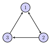
Figure 1: The communication topology of the generators.

5 Numerical simulations

In this section, a numerical example is provided to verify our established theoretical results. Consider a power system consisting of three generators with the communication topology shown in Fig. 1, which is a general unbalanced directed graph. Denote the active power generated by the three generators as x1,x2,x3subscript𝑥1subscript𝑥2subscript𝑥3x_{1},x_{2},x_{3}, respectively. From [15], the cost function of each generator can be generally approximated by: f1(x1)=0.096x12+1.22x1+51,subscript𝑓1subscript𝑥10.096superscriptsubscript𝑥121.22subscript𝑥151f_{1}(x_{1})=0.096x_{1}^{2}+1.22x_{1}+51, f2(x2)=0.072x22+3.41x2+31subscript𝑓2subscript𝑥20.072superscriptsubscript𝑥223.41subscript𝑥231f_{2}(x_{2})=0.072x_{2}^{2}+3.41x_{2}+31, and f3(x3)=0.105x32+2.53x3+78subscript𝑓3subscript𝑥30.105superscriptsubscript𝑥322.53subscript𝑥378f_{3}(x_{3})=0.105x_{3}^{2}+2.53x_{3}+78. The total load demand is 420420420MW, and the initial values x1(0)=x2(0)=x3(0)=140subscript𝑥10subscript𝑥20subscript𝑥30140x_{1}(0){=}x_{2}(0){=}x_{3}(0){=}140MW. The economic dispatch problem of the power system is to determine the active power supplied by each generator to minimize the total cost while meeting the total load demand, which can be described by

Minimizei=13fi(xi),Minimizesuperscriptsubscript𝑖13subscript𝑓𝑖subscript𝑥𝑖\displaystyle\mathrm{Minimize}\;\sum_{i=1}^{3}f_{i}(x_{i}), (34)
subjecttoi=13xi(t)=420MW.subjecttosuperscriptsubscript𝑖13subscript𝑥𝑖𝑡420MW\displaystyle\mathrm{subject}~{}~{}\mathrm{to}~{}\sum_{i=1}^{3}x_{i}(t)=420\text{MW}.
Refer to caption
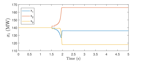
Figure 2: Evolution of x1,x2,x3subscript𝑥1subscript𝑥2subscript𝑥3x_{1},x_{2},x_{3} during 0s–5s.
Refer to caption
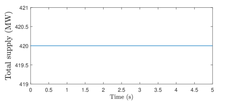
Figure 3: Evolution of the total supply i=13xisuperscriptsubscript𝑖13subscript𝑥𝑖\sum_{i=1}^{3}x_{i} during 0s–5s.
Refer to caption
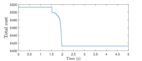
Figure 4: Evolution of the total cost i=13fisuperscriptsubscript𝑖13subscript𝑓𝑖\sum_{i=1}^{3}f_{i} during 0s–5s.
Refer to caption
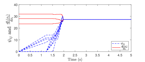
Figure 5: Evolution of ψijsubscript𝜓𝑖𝑗\psi_{ij} and dfi(xi)dxi𝑑subscript𝑓𝑖subscript𝑥𝑖𝑑subscript𝑥𝑖\frac{df_{i}(x_{i})}{dx_{i}} (i,j=1,2,3)formulae-sequence𝑖𝑗123(i,j{=}1,2,3) during 0s–5s.

To find the solution to problem (34) at the pre-specified time Tc=2subscript𝑇𝑐2T_{c}=2s, we use the proposed algorithm (3), which allows the agents exchange information only at some discrete-time instants. Arranged the sampling time sequence as (4) and (28) with kϵ=80subscript𝑘italic-ϵ80k_{\epsilon}=80, and ϵ=0.01italic-ϵ0.01\epsilon=0.01. The results are shown in Figs.2-5. The values of x1,x2,x3subscript𝑥1subscript𝑥2subscript𝑥3x_{1},x_{2},x_{3} and the total cost at 5s5𝑠5s are 135.9293135.9293135.9293, 166.0307166.0307166.0307, 118.0401118.0401118.0401 and 6412.1872836412.1872836412.187283 respectively, which are the same as the optimal solution found in [15]. Figs. 2 and 4 show that x1,x2,x3subscript𝑥1subscript𝑥2subscript𝑥3x_{1},x_{2},x_{3} and the total cost almost converge to the optimal values at the pre-specified time 222s respectively. To be more specific, the value of the total cost at 222s is 6412.1873976412.1873976412.187397, showing the high accuracy of the proposed specified-time distributed optimization algorithm with the modified Zeno-free sampling time sequence. Fig. 3 illustrates that the equality constraint in problem (34) is satisfied during the whole course. One can observe from Fig. 5 that ψij,dfidxi(xi),i,j=1,2,3formulae-sequencesubscript𝜓𝑖𝑗𝑑subscript𝑓𝑖𝑑subscript𝑥𝑖subscript𝑥𝑖𝑖𝑗123\psi_{ij},\frac{df_{i}}{dx_{i}}(x_{i}),i,j{=}1,2,3 reach consensus at 222s, which is in accordance with the theoretical analysis that the components of the gradient of the global objective function are equal to each other at the optimal point and the gradient estimation by each agent will converge to the actual gradient at the specified time.

6 Conclusion

In this paper, specified-time distributed optimization problem subject to the global equality constraint is investigated. A new distributed optimization algorithm is first proposed for general directed MANs, which can exactly reach the optimal solution at specified time under sampled-data communications. Under this algorithm, the settling time does not rely on algorithm parameters or communication topologies, which can be pre-assigned independently. For the special case of undirected MANs, a reduced-order distributed optimization algorithm is also designed, such that the computational cost would be greatly saved. Future work can be done to design specified-time distributed optimization algorithms for MANs with more practical constraints on decision variables.

References

  • [1] A. Nedić and J. Liu, “Distributed optimization for control,” Annual Review of Control, Robotics, and Autonomous Systems, vol. 1, pp. 77–103, 2018.
  • [2] T. Yang, X. Yi, J. Wu, Y. Yuan, D. Wu, Z. Meng, Y. Hong, H. Wang, Z. Lin, and K. H. Johansson, “A survey of distributed optimization,” Annual Reviews in Control, vol. 47, pp. 278–305, 2019.
  • [3] A. Nedić and A. Ozdaglar, “Distributed subgradient methods for multi-agent optimization,” IEEE Transactions on Automatic Control, vol. 54, no. 1, pp. 48–61, 2009.
  • [4] J. Lei, H. Chen, and H. Fang, “Primal-dual algorithm for distributed constrained optimization,” Systems and Control Letters, vol. 96, pp. 110–117, 2016.
  • [5] T. Yang, J. Lu, D. Wu, J. Wu, G. Shi, Z. Meng, and K. H. Johansson, “A distributed algorithm for economic dispatch over time-varying directed networks with delays,” IEEE Transactions on Industrial Electronics, vol. 64, no. 6, pp. 5095–5106, 2017.
  • [6] S. Pu, W. Shi, J. Xu and A. Nedic, “Push-pull gradient methods for distributed optimization in networks,” IEEE Transactions on Automatic Control, doi: 10.1109/TAC.2020.2972824.
  • [7] F. Guo, C. Wen, J. Mao, G. Li and Y. Song, “A distributed hierarchical algorithm for multi-cluster constrained optimization,” Automatica, vol. 77, pp. 230–238, 2017.
  • [8] F. Guo, C. Wen, J. Mao, J. Chen and Y. Song, “Hierarchical decentralized optimization architecture for economic dispatch: a new approach for large-scale power system,” IEEE Transactions on Industrial Informatics, vol. 14, no. 2, pp. 523–534, 2018.
  • [9] B. Gharesifard and J. Cortés, “Distributed continuous-time convex optimization on weight-balanced digraphs,” IEEE Transactions on Automatic Control, vol. 59, no. 3, pp. 781–786, 2014.
  • [10] J. Lu and C. Y. Tang, “Zero-gradient-sum algorithms for distributed convex optimization: the continuous-time case,” IEEE Transactions on Automatic Control, vol. 57, no. 9, pp. 2348–2354, 2012.
  • [11] W. Chen and W. Ren, “Event-triggered zero-gradient-sum distributed consensus optimization over directed networks,” Automatica, vol. 65, pp. 90–97, 2016.
  • [12] T. Yang, D. Wu, Y. Sun, and J. Lian, “Minimum-time consensus based approach for power system applications,”IEEE Transactions on Industrial Electronics, vol. 63, no. 2, pp. 1318–1328, 2016.
  • [13] V. S. Mai and E. H. Abed, “Local prediction for enhanced convergence of distributed optimization algorithms,” IEEE Transactions on Control of Network Systems, vol. 5, pp. 1962–1975, 2018.
  • [14] P. Lin, W. Ren, and J. A. Farrell, “Distributed continuous-time optimization: nonuniform gradient gains, finite-time convergence, and convex constraint set,” IEEE Transactions on Automatic Control, vol. 62, no. 5, pp. 2239–2253, 2017.
  • [15] G. Chen and Z. Li, “A fixed-time convergent algorithm for distributed convex optimization in multi-agent systems,” Automatica, vol. 95, pp. 539–543, 2018.
  • [16] B. Ning, Q. Han and Z. Zuo, “Distributed optimization for multiagent systems: an edge-based fixed-time consensus approach,” IEEE Transactions on Cybernetics, vol. 49, no. 1, pp. 122–132, 2019.
  • [17] W. Ren, R. W. Beard and E. M. Atkins, “Information consensus in multivehicle cooperative control,” IEEE Control Systems Magazine, vol. 27, no. 2, pp. 71–82, 2007.
  • [18] Y. Zhao, Y. Liu, G. Wen, W. Ren, and G. Chen, “Designing distributed specified-time consensus protocols for linear multiagent systems over directed graphs,” IEEE Trans. Autom. Control, vol. 64, no. 7, pp. 2945–2952, 2019.