Simulating gas giant exoplanet atmospheres with Exo-FMS:
Comparing semi-grey, picket fence and correlated-k radiative-transfer schemes.

Abstract

Radiative-transfer (RT) is a fundamental part of modelling exoplanet atmospheres with general circulation models (GCMs). An accurate RT scheme is required for estimates of the atmospheric energy transport and for gaining physical insight from model spectra. We implement three RT schemes for Exo-FMS: semi-grey, non-grey ‘picket fence’, and real gas with correlated-k. We benchmark the Exo-FMS GCM using these RT schemes to hot Jupiter simulation results from the literature. We perform a HD 209458b-like simulation with the three schemes and compare their results. These simulations are then post-processed to compare their observable differences. The semi-grey scheme results show qualitative agreement with previous studies in line with variations seen between GCM models. The real gas model reproduces well the temperature and dynamical structures from other studies. After post-processing our non-grey picket fence scheme compares very favourably with the real gas model, producing similar transmission spectra, emission spectra and phase curve behaviours. Exo-FMS is able to reliably reproduce the essential features of contemporary GCM models in the hot gas giant regime. Our results suggest the picket fence approach offers a simple way to improve upon RT realism beyond semi-grey schemes.

1 Introduction

The three dimensional (3D) atmospheric properties of hot Jupiters give rise to each of their unique spectral properties observed by contemporary telescopes and instrumentation technology. Understanding the 3D structure of these atmospheres and modelling them accurately is vital for a physical interpretation of their atmospheric dynamical and chemical characteristics. Recent studies have also shown the importance of considering the multi-dimensional nature of atmospheres when interpreting observational data (e.g. Feng et al., 2016; Dobbs-Dixon & Cowan, 2017; Blecic et al., 2017; Caldas et al., 2019; Irwin et al., 2020; Taylor et al., 2020). These studies suggest that neglecting the 3D nature of the atmosphere can lead to biased or inaccurate results when interpreting the thermal and molecular properties of the atmosphere.

During the operational lifetime of JWST it is expected that several phase curves observations of exoplanet atmospheres will be performed, providing wide infrared wavelength, detailed global atmospheric information. The Transiting Exoplanet Community Early Release Science (ERS) Program for JWST (Bean et al., 2018; Venot et al., 2020) plans to observe phase curves of the hot Jupiter WASP-43b. In addition, the Transiting Exoplanet Survey Satellite (TESS) (Ricker et al., 2014), CHaracterising ExOPlanet Satellite (CHEOPS) (Broeg et al., 2013) and the high altitude ballon mission EXoplanet Climate Infrared TElescope (EXCITE) (Nagler et al., 2019) are able to observe several phase curves of hot Jupiters in the optical and infrared wavelength regimes. Recently, TESS data on the phase curves of WASP-18b (Shporer et al., 2019) and WASP-19b (Wong et al., 2020a), WASP-121b (Daylan et al., 2021; Bourrier et al., 2020), WASP-100b (Jansen & Kipping, 2020) and KELT-9b (Wong et al., 2020b) have been published. As more phase curve data of nearby characterisable planets becomes available, a larger census of the dynamical properties of hot Jupiter atmospheres, as well as their cloud coverage through dayside albedo constraints (e.g. Cahoy et al., 2010; Barstow et al., 2014; Garcia Munoz & Isaak, 2015; Parmentier et al., 2016; Batalha et al., 2019; Mayorga et al., 2019) will become possible. The Atmospheric Remote-sensing Infrared Exoplanet Large-survey (ARIEL) (Tinetti et al., 2016) telescope is also scheduled to perform numerous phase curve observations of hot gas giant planets (Charnay et al., 2021).

High resolution spectroscopy observations have also helped reveal the rich chemical inventory of hot Jupiter atmospheres (e.g. Seidel et al., 2019; Ehrenreich et al., 2020; Merritt et al., 2020; Pino et al., 2020). 3D modelling efforts have shown that considering the 3D structures in detail affects the interpretation of high resolution transmission spectra results (e.g. Miller-Ricci Kempton & Rauscher, 2012; Flowers et al., 2019). Possible improvements in the molecular detection significance for high resolution emission spectra using GCM model output as a template has also been reported in Beltz et al. (2021).

The 3D modelling of hot Jupiter (HJ) atmospheres using large scale simulation platforms has become an important toolkit in understanding the physical processes that give rise to the observational characteristics of these planets (Showman et al., 2020). Several groups have examined hot Jupiter (HJ) and warm Neptune atmospheres with 3D General Circulation Models (GCMs) or Radiative-Hydrodynamic (RHD) models, for example, Showman et al. (2009); Rauscher & Menou (2010); Heng et al. (2011a); Dobbs-Dixon & Agol (2013); Mayne et al. (2014); Charnay et al. (2015); Mendonça et al. (2016). Each of these models generally produce qualitatively similar dynamical structures (Heng & Showman, 2015), despite many differences in their implementations, the level of simplification from the Navier-Stokes equations, numerics, 3D grid structure, vertical coordinate system to radiative-transfer scheme.

Radiative-transfer (RT) is a key component in GCM models, controlling the heating and cooling in the atmosphere which majorly impacts the dynamical properties of the atmosphere. Due to their importance, significant effort has been made developing a broad spectrum of RT schemes in the literature. Equilibrium relaxation or simplified RT approaches such as Newtonian relaxation (e.g. Showman et al., 2008; Rauscher & Menou, 2010; Heng et al., 2011a; Mayne et al., 2014; Carone et al., 2020) and multi-band grey or non-grey schemes of various flavours (e.g. Heng et al., 2011b; Rauscher & Menou, 2012; Dobbs-Dixon & Agol, 2013; Mendonça et al., 2018) are commonly used in HJ GCM modelling. These efficient schemes have enabled easier model inter-comparison (Heng & Showman, 2015) and larger parameter explorations (e.g. Komacek & Showman, 2016; Komacek et al., 2017; Tan & Komacek, 2019; Tan & Showman, 2020) in an effort to understand dynamical regime changes. Detailed real gas, correlated-k RT models have also been coupled to GCMs (e.g. Showman et al., 2009; Charnay et al., 2015; Amundsen et al., 2016), providing a more realistic but more costly RT solution. Several targeted object simulations (Kataria et al., 2014, 2016; Amundsen et al., 2016) and parameter explorations (Parmentier et al., 2016) have been performed using correlated-k modelling. Recently, Ding & Wordsworth (2019) implemented a line-by-line RT approach in their GCM to model the atmosphere of GJ 1132b. Similar RT schemes are also a key component for GCM and general atmospheric modelling for Solar System planets. Many RT models have been developed, such as for Venus (e.g. Lebonnois et al., 2010; Mendonça et al., 2015; Mendonça & Read, 2016; Limaye et al., 2018) and for Jupiter (e.g. Schneider & Liu, 2009; Kuroda et al., 2014; Li et al., 2018; Young et al., 2019).

In this study, we couple three different RT schemes to the 3D Exo-FMS GCM model, and benchmark them to several hot Jupiter models performed in the literature. Exo-FMS has been previously used to model condensable rich atmospheres on terrestrial planets (Pierrehumbert & Ding, 2016), explore atmospheric compositions of 55 Cnc e (Hammond & Pierrehumbert, 2017) and the White dwarf - Brown dwarf short period binary WD0137-349B (Lee et al., 2020), showcasing Exo-FMS flexibility and applicability to model and explore a wide planetary parameter space. We benchmark to commonly used set-ups for hot Jupiter modelling efforts and examine our semi-grey, non-grey picket fence and real gas RT models for a HD 209458b test case. In Sect. 2 we summarise the Exo-FMS hydrodynamic and radiative-transfer methods. In Sect. 4 we present benchmarking results using the semi-grey RT scheme. In Sect. 5.1, 5.2 and 5.3 we present HD 209458b-like simulations using the semi-grey, non-grey picket fence and real gas RT schemes respectively. The differences in each model are examined in Sect. 5.4. Section 6 presents transmission, emission and phase curve post-processing of the HD 209458b-like results and comparisons between the three models and available observational data. Section 7 contains the discussion of our results and Sect. 8 contains the summary and conclusions.

2 Exo-FMS

Exo-FMS is a GCM adapted from the Princeton Geophysical Fluid Dynamics Laboratory (GFDL) Flexible Modelling System (FMS). Other groups have also used the FMS framework for exoplanet studies, such as the ISCA model (e.g. Thomson & Vallis, 2019) which uses a spectral dynamical core, and the Heng et al. (2011a), Heng et al. (2011b) and Oreshenko et al. (2016) studies.

In the current Exo-FMS version, we use the finite volume dynamical core (Lin, 2004). A key advantage of this version of Exo-FMS is the scalability afforded by the cube sphere implementation, increasing the efficiency of computationally demanding physics such as real gas radiative-transfer, chemical kinetics and cloud formation. The cube-sphere grid also avoids singularities at the pole regions, a common problem with lat-lon based grids. In this study we use a resolution of C48, $\approx$ 192 $\times$ 96 in longitude $\times$ latitude. C48 is typically higher than the C32 resolution commonly used by SPARC/MITgcm (e.g. Parmentier et al., 2021), C32 was found to capture most of large scale dynamical flows of hot Jupiter atmospheres (e.g. Showman et al., 2009).

Exo-FMS uses a hybrid-sigma vertical pressure grid system, where deep regions are typically spaced in log-pressure starting from a ‘surface’ reference pressure (here 220 bar), with a gradual transition to more linear spacing occurring at lower pressure. We generally use a 53 level grid with a lowest pressure of $10^{-6}$ bar, with more linear spacing starting at $\lesssim$ 10^-3 bar.

2.1 Hydrodynamics

Exo-FMS evolves the standard primitive equations of meteorology, extensively detailed in many textbooks and sources, for example, Holton & Hakim (2013), Mayne et al. (2014), Heng (2017) and Mayne et al. (2019). We note that there are indications that the use of primitive equations for the slow rotating warm Neptune regime can lead to significant errors in the wind field, especially near the equatorial regions (Mayne et al., 2019). These appear to be due to geometric terms conventionally neglected in the primitive equations, rather than the hydrostatic approximation itself. However, the primitive equation set assumptions are well met in the hot Jupiter regime (Mayne et al., 2014).

2.2 Dry convective adjustment

Dry convective adjustment is included using a layerwise enthalpy conserving scheme. Convective adjustment is given by examining layer $i$ for the criteria

$$T_{i}<T_{i+1}\left(\frac{p_{i}}{p_{i+1}}\right)^{\kappa},$$ (1)

where $\kappa$ = $R_{\rm atm}$/$c_{\rm p}$, the specific gas constant divided by the specific heat capacity at constant pressure of the atmosphere. The layer pair are then adjusted to the adiabatic gradient while conserving dry enthalpy. This processes is iterated until no pair of layers are convectively unstable and the whole column is stable.

2.3 Semi-grey radiative transfer

In a semi-grey RT scheme, the irradiation by the host star (shortwave radiation) is represented by a single ‘visual’ (V) band, with a characteristic constant opacity. Similarly for the internal atmospheric thermal ‘infrared’ (IR) fluxes (longwave radiation), a single band with a characteristic opacity is also used. It is important to note that the V and IR bands do not necessarily conform to strict visual and infrared wavelength regimes.

In a two-stream context this simplifies the RT scheme to performing two sets of calculations: the downward (and sometimes upward) flux resulting from stellar irradiation, and the downward and upward thermal band fluxes. Below we briefly summarise the main components.

2.3.1 Shortwave radiation

The flux at the sub-stellar point received by the planet by its host star, $F_{0}$ [W m^-2], is given by the irradiation temperature, $T_{\rm irr}$ [K], (e.g. Guillot, 2010)

$$F_{0}=\sigma T_{\rm irr}^{4}=\sqrt{\frac{R_{\star}}{a}}\sigma T_{\star}^{4},$$ (2)

where $\sigma$ [W m^-2 K^-4] is the Stefan-Boltzmann constant, $R_{\star}$ [m] the radius of the host star, $a$ [m] the orbital semi-major axis and $T_{\star}$ [K] the effective temperature of the host star. For an atmosphere that is purely absorbing in the shortwave band, the reference shortwave optical depth $\tau_{S_{0}}$ is calculated, assuming hydrostatic equilibrium, given by

$$\tau_{S_{0}}=\frac{\kappa_{v}p_{0}}{g},$$ (3)

where $\kappa_{v}$ [m² g^-1] is the grey visual band opacity, $p_{0}$ [pa] the reference surface pressure and g [m s^-2] the surface gravity. The cumulative optical depth at each vertical cell level for a constant with height opacity source is then

$$\tau_{i}=\tau_{S_{0}}\frac{p_{i}}{p_{0}},$$ (4)

where p_i [pa] is the pressure at the cell interface. The downward shortwave flux, $F_{\downarrow S}$ [W m^-2], at each vertical level is then

$$F_{\downarrow S}=(1-A_{B})\mu_{\star}F_{0}\exp(-\tau_{i}/\mu_{\star}),$$ (5)

where $\mu_{\star}$ = $\cos(\phi)\cos(\theta)$ is the cosine angle from the sub-stellar point and A_B a parametrised Bond albedo.

The optical wavelength scattering properties of the atmosphere are implicitly included in the A_B parametrisation. For a purely absorbing atmosphere, the Bond albedo would be zero, but here, in line with common practice, we introduce an imposed albedo as an approximation to the effects of scattering. It would be straightforward and still computationally efficient to introduce a two-stream formulation including scattering for the shortwave band, but since our object here is benchmarking against published results in the simplest possible way, we have retained the commonly used expedient of forcing the atmosphere with pure direct beam absorption and top-of-atmosphere flux adjusted according to an assumed albedo. The effects of multiple scattering would alter the vertical distribution of heating, and in particular scatter direct beam into diffuse radiation, reducing the dependence on zenith angle (Pierrehumbert, 2010).

2.3.2 Longwave radiation

For the longwave fluxes, we follow a simplified version of the scheme presented in Toon et al. (1989). Ignoring the coupling coefficients for scattering (i.e. in the w₀ $\rightarrow$ 0 limit) the two-stream formulation reduces to

$$I_{\uparrow 1}=I_{\uparrow 2}T_{0}+2\pi B_{2}(1-T_{0})+2\pi B^{\prime}[\mu-(\Delta+\mu)T_{0}],$$ (6)

for the upward intensity, $I_{\uparrow}$ [W m^-2 sr^-1], and

$$I_{\downarrow 2}=I_{\downarrow 1}T_{0}+2\pi B_{1}(1-T_{0})+2\pi B^{\prime}[\mu T_{0}+\Delta+\mu],$$ (7)

for the downward intensity, $I_{\downarrow}$ [W m^-2 sr^-1], with $\mu$ the emission angle. We follow the notation of Heng et al. (2018) with level 2 located below 1 in altitude, with $\Delta$ = $\tau_{2}$ - $\tau_{1}$ $>$ 0,

$$T_{0}=\exp\left(-\Delta/\mu\right),$$ (8)

the transmission function, and B^′ = (B₂ - B₁)/$\Delta$ the linear in $\tau$, non-isothermal layer blackbody term. For very small optical depths the above scheme can become numerically unstable, we therefore switch to an isothermal approximation when the optical depth becomes small. When layers have $\Delta$ $<$ 10^-6 the upward and downward intensity are given by

$$I_{\uparrow 1}=I_{\uparrow 2}T_{0}+\pi(B_{2}+B_{1})(1-T_{0}),$$ (9)

and

$$I_{\downarrow 2}=I_{\downarrow 1}T_{0}+\pi(B_{2}+B_{1})(1-T_{0}),$$ (10)

respectivly. For grey schemes, the blackbody intensity in the above equations is given by the wavelength integrated blackbody intensity, B = $\sigma$T⁴/$\pi$ [W m^-2 sr^-1]. The flux at each level is then calculated by quadrature integration of different $\mu$ values. In this study we use two quadrature angles, which was found to give similar quality results to higher numbers of quadrature points, Appendix A, (e.g. Lacis & Oinas, 1991).

The upward and downward longwave fluxes $F_{L}$ [W m^-2] at each level are then given by

$$F_{\uparrow L}=\sum_{g}^{2}w_{g}\mu_{g}I_{\uparrow,g}\\ F_{\downarrow L}=\sum_{g}^{2}w_{g}\mu_{g}I_{\downarrow,g},$$ (11)

where w_g is quadrature weight and $\mu_{g}$ the emission angle.

The net flux into and out of the cell level is then

$$F_{\rm net}=F_{\uparrow L}-F_{\downarrow L}-F_{\downarrow S},$$ (12)

with the flux from the deep interior is modelled as a net flux at the deepest level given by the internal temperature, T_int [K],

$$F_{\rm net,int}=\sigma T_{\rm int}^{4}.$$ (13)

The temperature tendency due to radiative heating/cooling, $\partial$T/$\partial$t [K s^-1], is then given by

$$\frac{\partial T}{\partial t}=\frac{g}{c_{\rm p,air}}\frac{\partial F_{\rm net}}{\partial p},$$ (14)

where g [m s^-2] is the surface gravity and c_p,air [J kg^-1 K^-1] the heat capacity of the air.

In the semi-grey scheme, the longwave optical depth at each cell interface is given following Heng et al. (2011a)

$$\tau_{i}=f_{l}\tau_{L_{0}}\frac{p_{i}}{p_{0}}+(1-f_{l})\tau_{L_{0}}\left(\frac{p_{i}}{p_{0}}\right)^{n_{L}},$$ (15)

where $f_{l}$ is the fraction between the constant (linear term) which represents molecular and atomic line opacity and exponent term, $\tau_{L_{0}}$ the reference longwave optical depth and $n_{L}$ the pressure dependence exponent, representing collision-induced continuum opacity.

2.4 Non-grey picket fence scheme

As an intermediate model between the semi-grey and real gas RT models we develop a non-grey ‘picket fence’ RT approach (Chandrasekhar, 1935) based on Parmentier & Guillot (2014) and Parmentier et al. (2015). The picket fence scheme attempts to more accurately model the propagation of radiation through the atmosphere by the use of two opacities, one representing the molecular and atomic line opacity and one representing the general continuum opacity. The value of these opacities are linked to the local temperature and pressure dependent Rosseland mean opacity through fitting functions derived analytically in Parmentier & Guillot (2014); Parmentier et al. (2015) and tuned to best fit the results of a correlated-k model for each value of T_eff. In addition to this, Parmentier et al. (2015) use additional V band opacity relations to better capture the deposition of incident stellar flux. The key concepts from Parmentier & Guillot (2014); Parmentier et al. (2015) applied here are the use of three V bands and two picket fence IR bands (again these bands do not strictly correspond to optical and infrared wavelength regimes).

The optical depth contribution in each layer, $\Delta\tau_{i}$, assuming hydrostatic equilibrium, is given by

$$\Delta\tau_{i}=\frac{\kappa_{i}(p_{i},T_{i})}{g}\Delta p_{i},$$ (16)

where $\kappa_{i}$ [m² g^-1] is the opacity of the layer, now dependent on the local pressure and temperature, g [m s^-2] the gravitational acceleration and $\Delta p_{i}$ [pa] the difference in pressure between the cells lower and upper level respectively. The value of $\kappa_{i}$ is calculated in each layer for each V and IR band as function of the local Rosseland mean opacity, $\kappa_{R}$ [m² g^-1], given by

$$\frac{1}{\kappa_{R}}=\frac{\int^{\infty}_{0}\frac{1}{\kappa_{\lambda}}\frac{dB_{\lambda}}{dT}d\lambda}{\int^{\infty}_{0}\frac{dB_{\lambda}}{dT}d\lambda},$$ (17)

where $\kappa_{\lambda}$ [m² g^-1] is the wavelength dependent opacity and dB_λ/dT the temperature derivative of the Planck function, and opacity ratio coefficients, $\gamma_{i}$, (Parmentier & Guillot, 2014; Parmentier et al., 2015) through the relation

$$\gamma_{i}=\frac{\kappa_{i}}{\kappa_{R}}.$$ (18)

The downward V band flux is now calculated as a sum of the downward stellar flux calculations with opacities $\kappa_{V,i}$

$$F_{\downarrow S}=(1-A_{B})F_{0}\mu_{\star}\sum_{b}^{N_{b}}\beta_{V,b}\exp(-\tau_{i,b}/\mu_{\star}),$$ (19)

where $N_{b}$ is the number of V bands (here three), $\beta_{V,b}$ the fraction of stellar flux in band $b$ (here 1/3) and A_B the Bond albedo. The value of A_B can be calculated from the fitting function presented in Parmentier et al. (2015) or given as a parameter.

For the longwave flux calculations, the picket fence model considers two bands, with opacities $\kappa_{1}$ and $\kappa_{2}$, each with a fraction $\beta$ of the integrated blackbody flux. Equations 6 and 7 are performed twice, one with opacity $\kappa_{1}$ and $\beta$B and one with $\kappa_{2}$ and (1 - $\beta$)B, the flux of both bands are then summed to find the net flux.

Following Parmentier & Guillot (2014); Parmentier et al. (2015) we define the effective temperature, T_eff [K], of an individual vertical profile as

$$T_{\rm eff}^{4}=T_{\rm int}^{4}+(1-A_{B})\mu_{\star}T_{\rm irr}^{4},$$ (20)

where $\mu_{\star}$ is the cosine angle of the column from the sub-stellar point, A_B the Bond albedo, T_irr [K] the substellar point irradiation temperature and T_int [K] the internal temperature. For nightside profiles T_eff = T_int.

On a practical level, the scheme operates as follows:

1. Calculate the Bond albedo following the Parmentier et al. (2015) expression, with T_eff assuming $\mu_{\star}$ = 1/$\sqrt{3}$.

2. Calculate the $\gamma_{v1}$, $\gamma_{v2}$, $\gamma_{v3}$, $\beta$, $\gamma_{p}$ and R = $\kappa_{1}/\kappa_{2}$ constants from the profile T_eff for each column’s $\mu_{\star}$, Eq. 20, following the fitting coefficient tables in Parmentier et al. (2015) and definitions in Parmentier & Guillot (2014).

3. Find the IR band Rosseland mean opacity, $\kappa_{R}$ (p,T), in each layer from the Freedman et al. (2014) fitting function.

4. Find the three V band opacities in each layer using the $\gamma_{v1}$, $\gamma_{v2}$, $\gamma_{v3}$ and $\kappa_{R}$ relationships.

5. Find the two IR band opacities in each layer using the $\kappa_{1},\kappa_{2}$ and $\gamma_{P}$, $\beta$, R relationships.

6. Calculate the vertical optical depth structure and perform the two-stream calculations for each V and IR band.

Each column in the GCM has a constant T_eff as defined by this scheme, so the Parmentier et al. (2015) parameters need only be calculated once at the start of the simulation. The $\gamma_{v1}$, $\gamma_{v2}$, $\gamma_{v3}$, $\beta$, $\gamma_{p}$ and R = $\kappa_{1}/\kappa_{2}$ constants were parametrised in Parmentier et al. (2015) to match the T-p profiles of the Fortney et al. (2005) and collaborators 1D radiative-convective equilibrium (RCE) model across a wide variety of T_eff. In essence, the these parameters produce opacity structures, combined with the dry convective adjustment scheme, that tend each column to the analytical RCE T-p profiles given by Parmentier et al. (2015), with the energy transport timescales from the atmospheric dynamics giving rise to the non-equilibrium behaviour of the 3D temperature structures.

Overall, this picket fence scheme attempts to add more realism than semi-grey case, at the cost of now performing 3 shortwave flux calculations and 2 longwave flux calculations as well as calculating Rosseland mean opacities. This model is therefore typically $\approx$2-3 times more computationally expensive than the semi-grey calculation, but presents a more physical way of representing the thermal structure of the atmosphere as opacities are now able to adapt to the local temperature and pressure variations. In addition, collision-induced absorption opacities are included in the Rosseland mean calculation resulting in a more accurate representation of the pressure dependence of the opacity structure without relying on tuning the pressure dependent exponent in the semi-grey scheme.

2.5 Real gas radiative transfer

Table 1: Opacity sources and references used in the GCM correlated-k scheme and cmcrt post-processing. ‘NU’ denotes ‘not used’.

Opacity Source	GCM model / CMCRT post-processing
Line	Reference
Na	Kurucz & Bell (1995)/Kramida et al. (2013)
K	Kurucz & Bell (1995)/Kramida et al. (2013)
H2O	Polyansky et al. (2018)
CH4	Yurchenko et al. (2017)
C2H2	Chubb et al. (2020)
NH3	Coles et al. (2019)
CO	Li et al. (2015)
CO2	Rothman et al. (2010)
H2S	Azzam et al. (2016)/NU
HCl	Gordon et al. (2017)/NU
HCN	Harris et al. (2006); Barber et al. (2014)/NU
SiO	Barton et al. (2013)/NU
PH3	Sousa-Silva et al. (2015)
TiO	McKemmish et al. (2019)/NU
VO	McKemmish et al. (2016)/NU
MgH	GharibNezhad et al. (2013)/NU
CaH	Bernath (2020)/NU
TiH	Bernath (2020)/NU
CrH	Bernath (2020)/NU
FeH	Bernath (2020)/NU
Continuum
H2-H2	Karman et al. (2019)
H2-He	Karman et al. (2019)
H2-H	Karman et al. (2019)
H-He	Karman et al. (2019)
H-	John (1988)
He-	Kurucz (1970)
Rayleigh scattering
H2	Dalgarno & Williams (1962)
He	Thalman et al. (2014)
H	Kurucz (1970)
e-	Thompson scattering

For our real gas radiative scheme, we use the same two-stream formulations as in Sect. 2.3.2 for a fair comparison to the grey and picket fence schemes, with modifications to use the 30 wavelength band structure from Showman et al. (2009). We produce k-coefficient tables using the high resolution opacities from HELIOS-K (Grimm & Heng, 2015; Grimm et al., 2021) with Na and K opacities from Kitzmann et al. (2020). We use the same k-coefficient Gaussian ordinance nodes (4+4 split between 0-0.95 and 0.95-1.0 Kataria et al. (2013)).

We implement pre-mixed opacities where the high resolution opacities of each species are combined offline and weighted by the mixing ratio of each gas before calculating the k-coefficients across a grid of temperature and pressure points (Showman et al., 2009; Amundsen et al., 2017). GGchem (Woitke et al., 2018) is used to calculate the species mixing ratios assuming chemical equilibrium with equilibrium condensation included. Solar metallicity is assumed using the element ratios presented in Asplund et al. (2009). Rayleigh and collision-induced absorption opacities are also added to each band separately during runtime. Table 1 contains references for the opacities used in the current study.

We use the pysynphot package (STScI Development Team, 2013) to calculate the incident stellar flux in each band. The Phoenix database (Allard et al., 2011) was interpolated to the properties of HD 209458 (T_eff = 6092 K, R_⋆ = 1.203 R_⊙ - exoplanet.eu) as the input stellar model.

2.5.1 Gas phase abundances

For the current pre-mixed scheme, since the k-table is already weighted by the VMR of each species offline, only the species for the CIA and Rayleigh opacities are required to calculated inside the GCM during runtime. We use an interpolation from a 2D grid calculated using GGchem including the effects of local equilibrium condensation. Solar metallicity is assumed using the element ratios presented in Asplund et al. (2009). This grid ranges from 691 points in temperature between 100-7000 K in steps of 10 K and 91 pressure points log-spaced between 10^-6-1000 bar. Additionally, we also interpolate the local mean molecular weight from the CE calculation for use in the RT scheme.

3 Initial condition considerations

Figure 1: Exo-FMS output of the fiducial Heng et al. (2011b) hot Jupiter simulation parameters. Top left: 1D T-p profiles at the equator (solid coloured lines) and polar region (black dashed line). Top right: Zonal mean gas temperature. Bottom left: Lat-lon map of the OLR flux. Bottom right: Zonal mean zonal velocity.

An important consideration, especially for the evolution of the deep layers is the GCM initial conditions (ICs). We therefore propose a new IC scheme for our three HD 209458b simulations in Sect. 5.

Recently, Sainsbury-Martinez et al. (2019) suggest that the deep atmospheric regions of hot Jupiters tend to evolve to a hot adiabatic profile due to dynamical mixing between the deep and upper layers. In their models, they found that isothermal ICs gradually evolve towards a deep adiabatic profile over long timescales. They suggest that a hot adiabatic IC for HJ GCMs should be considered to better capture this long term evolution, as a hotter profile can more quickly cool towards the true adiabatic gradient, compared to a cooler gradient warming up.

Thorngren et al. (2019) published an expression to relate the incident flux and internal temperature in order to fit the observed radii of the hot Jupiter population. This greatly affects the thermal structure of the deep atmosphere, with larger T_int increasing the steepness of the T-p structure.

Bearing these studies in mind, we initialise each 1D GCM column in our HD 209458b tests using the Parmentier & Guillot (2014); Parmentier et al. (2015) analytical T-p expressions at the sub-stellar point ($\mu_{\star}$ = 1) with their adiabatic correction scheme. Using the sub-stellar point profile ensures that the adiabatic region will be slightly too hot initially for most of the atmosphere, allowing the suggestion of Sainsbury-Martinez et al. (2019) to be implemented in a simple manner. The T_int value (here 571 K for HD 209458b) is calculated using the Thorngren et al. (2019) expression of the internal temperatures of the hot Jupiter population as a boundary condition for the IC scheme as well as setting the internal flux for the RT scheme.

4 Semi-Grey RT results

In this section, we present results using the Exo-FMS semi-grey RT scheme, benchmarking to the Heng et al. (2011b) and Rauscher & Menou (2012) studies that both used a semi-grey RT approach.

4.1 Heng et al. (2011) benchmark

In Heng et al. (2011b) simulations were performed with the FMS spectral dynamical core including a grey gas RT scheme. Since their experiments used a similar framework to our current study, Heng et al. (2011b) is the most comparable simulation to the current study. We perform the fiducial hot Jupiter model with the parameters found in Heng et al. (2011b, Table. 1). We alter the grey RT in Sect. 2.3 to conform to the same scheme in Heng et al. (2011b). An isothermal initial condition at 1824 K is used with T_int = 0 K internal temperature. The simulation is run for 3600 (Earth) days, with the final 100 day average presented as the results in this study.

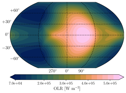
Figure 1 presents our benchmarking results to Heng et al. (2011b). The zonal mean wind and temperature structures closely match the results of Heng et al. (2011b). The wind has a peak value of 5500 m s^-1 occurring near 0.1 bar in both cases, and the jet widths are similar. The temperature hot spot is 1800 K occurring near 1 bar in both cases, and the horizontal pattern of OLR, which is an important signature of wave dynamics, agrees closely with Heng et al. (2011b). Both simulations show prominent Rossby wave cold cyclones straddling the equator to the west of the substellar point. This structure is an important indicator of the effect of the jet on the wave dynamics (Hammond & Pierrehumbert, 2018). The GCM in Heng et al. (2011b) used the spectral dynamical core and here the cube sphere, finite volume version. This is an indication the Exo-FMS dynamical core is producing comparable flow patterns compared to contemporary models.

The agreement in jet structure is notable in view of the very different dynamical cores used in the two simulations and demonstrates that the use of the cube sphere grid has not distorted the relevant angular momentum transport processes, since the jet speed is sensitive to angular momentum transport (Mendonça, 2020).

Angular momentum transport plays a crucial role in the generation of super-rotation, and problems with angular momentum conservation have been implicated as a cause of intermodal differences in reproducing the superstation of Venus (Lee & Richardson, 2012). The FMS spectral dynamical core has been found to conserve angular momentum in Venus test cases to within 2$\%$ per century (Lee & Richardson, 2012). However, the momentum conservation properties for the hot Jupiter class of exoplanets is different to that of Venus. Polichtchouk et al. (2014) discuss the differences in momentum conservation between GCM models in a hot Jupiter context, and included the MITgcm cubed-sphere dynamical core in their analysis. However, the FMS cube-sphere (or spectral) dynamical cores were not compared in Polichtchouk et al. (2014), which has different numerical schemes to MITgcm. The good agreement between our FMS cube-sphere simulations and the Heng et al. (2011b) spectral benchmark is a reassuring indication that the cube sphere dynamical core can adequately reproduce the necessary angular momentum transport properties, at least in the context of tide-locked circulations. However, this is not a rigorous test of the conservation properties of the current model. With our additions to Exo-FMS in this paper, a more substantive intercomparison, similar to that of Polichtchouk et al. (2014), can be performed in hot Jupiter context in future dedicated investigations.

4.2 Rauscher & Menou (2012) benchmark

Figure 2: Exo-FMS output of the hot Jupiter simulation presented in Rauscher & Menou (2012). Top left: 1D equatorial T-p profiles (solid colour lines) and polar region (black dashed line). The dash-dot lines show the sub-stellar (orange) and self-luminous (cyan) radiative-equilibrium solutions from Guillot (2010). Top right: zonal mean zonal velocity. Bottom left: lat-lon map of gas temperature with velocity vectors (black arrows) near the photosphere ($\approx$ 51 mbar). Bottom right: lat-lon map of the OLR flux.

In Rauscher & Menou (2012) several double-grey RT models were performed to examine the effects of magnetic drag on the dynamical properties of hot Jupiter exoplanets. The model used in Rauscher & Menou (2012), like that in Heng et al. (2011b), employs a spectral dynamical core, but derives from an independently developed model with somewhat different formulation of the primitive equations, in long use for Earth climate studies. We perform a similar simulation to their fiducial model present in Table. 1 of Rauscher & Menou (2012). Rauscher & Menou (2012) include a flux limited diffusion scheme for longwave radiation at high optical depths. As in Rauscher & Menou (2012) we initialise the model with Milne’s T-p profile solution for self-luminous objects (e.g. Guillot, 2010; Heng et al., 2014) with T_int = 500 K.

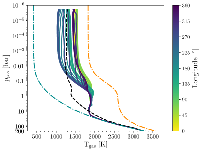
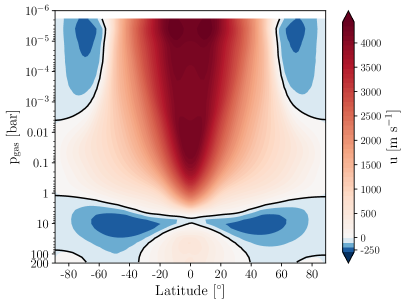
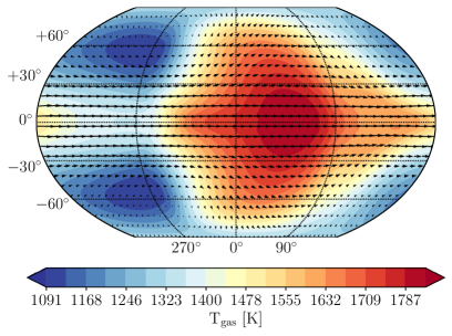
In Fig. 2 we present the results of our Exo-FMS run using the Rauscher & Menou (2012) simulation parameters. Results are taken after 3600 days of simulation, with the final 100 day average used as the presented results. The qualitative features of the atmospheric state agree with our simulation, in that there is a super-rotating equatorial jet which decays with depth in the atmosphere, a hot-spot in the OLR which is shifted eastward relative to the sub-stellar point, and a pronounced dayside-nightside temperature difference in the upper atmosphere (as seen in the profiles). However, there are a number of significant quantitative differences. The jet maximum in Rauscher & Menou (2012) is about 2000 m s^-1 stronger, and the jet penetrates deeper into the atmosphere (about 10 bars vs. about 3 bars in our case). The nightside equatorial temperature profiles agree well between the two simulations, but the dayside temperature in Rauscher & Menou (2012) has a peak of 2200 K at 0.5 bars, whereas our simulation is monotonic in the upper atmosphere and several hundred K cooler at the 0.5 bar level, however, the dayside temperatures in the far upper atmosphere agree reasonably well between the simulations. Another quantitative difference is that the hot-spot shift is approximately 25 degrees in Rauscher & Menou (2012), vs. 50 degrees in our simulation.

Because Exo-FMS simulations check out well against the Heng et al. (2011b) simulations, which like Rauscher & Menou (2012) employed a spectral dynamical core, we think it unlikely that the quantitative differences arise from the dynamical core. Although we have set the grey parameters in our radiative scheme to mimic Rauscher & Menou (2012) as closely as possible, the differences in the formulation of the radiation scheme make an exact match impossible. This disparity most likely stems from the differences in the RT scheme used between the models, with Rauscher & Menou (2012) switching to a diffusion approximation at high IR optical depths, whereas we use a two-stream approach with a linear in tau term (Sect. 2.3.2). Differences in the cooling/heating rates leads a variance in the dynamical forcing between the models, however, it is difficult in practice to diagnose the exact reason for the different results. We take the discrepancies as an indication that even within the scope of semi-grey radiation, differences in the formulation can lead to significantly different results.

5 HD 209458b-like simulations

In this section we perform HD 209458b-like simulations, similar to those in Showman et al. (2009). The simulation in Showman et al. (2009) employs the MITgcm dynamical core, which, like Exo-FMS, uses a cube-sphere grid with finite-volume numerics, though it is coded independently from Exo-FMS and involves somewhat different numerical algorithms. This simulation is then run using the semi-grey, non-grey picket fence and a correlated-k model. The difference between each model are then compared and examined on how each RT scheme affected the end results. The parameters used in each experiment can be found in Appendix B.

5.1 Semi-grey RT results

Figure 3: Exo-FMS output of a HD 209458b-like experiment using the semi-grey RT scheme. Top left: 1D equatorial T-p profiles (solid colour lines) and polar region (black dashed line). Top right: zonal mean zonal velocity. Middle left: lat-lon map of gas temperature at $\approx$1 mbar. Middle right: lat-lon map of gas temperature at $\approx$10 mbar. Bottom left: lat-lon map of gas temperature at $\approx$0.1 bar. Bottom right: lat-lon map of gas temperature at $\approx$1 bar. Velocity vectors are shown as back arrows.

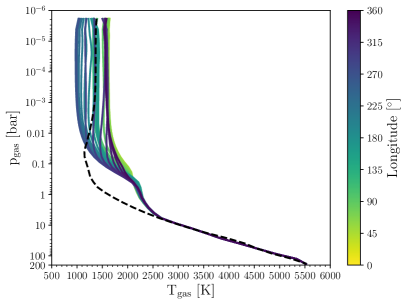
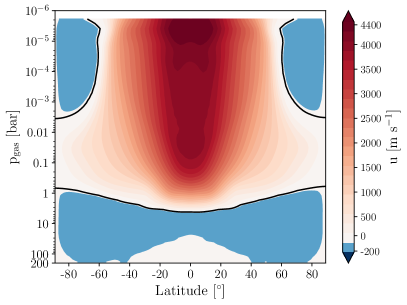
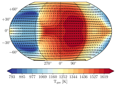
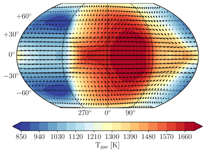
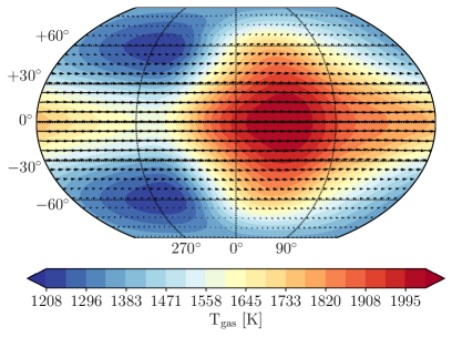
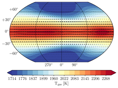
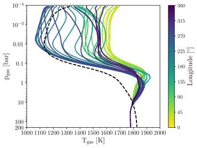
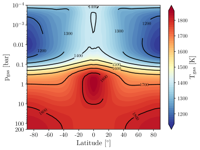
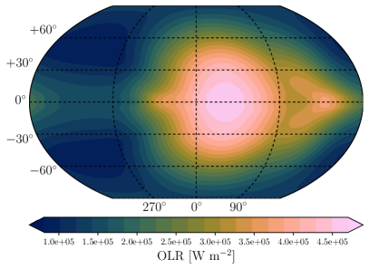
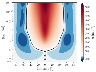
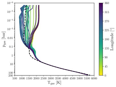
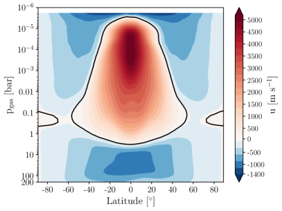
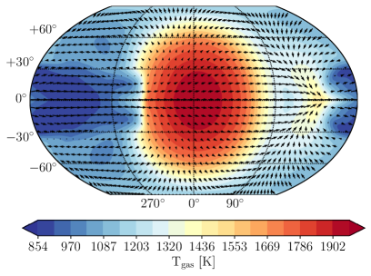
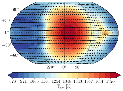
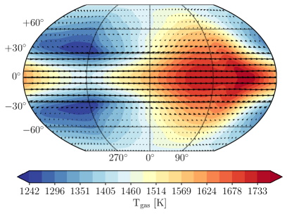
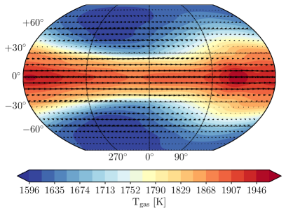
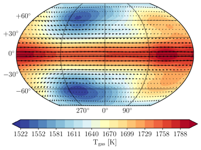
In this simulation we use the semi-grey RT scheme for the HD 209458b-like simulation. For the semi-grey opacities, we use the Guillot (2010) values of $\kappa_{IR}$ = 10^-3 [m² kg^-1] and $\kappa_{V}$ = 6 $\times$ 10^-4 $\times$ $\sqrt{T_{\rm irr}/2000}$ = 6.14 $\times$ 10^-4 [m² kg^-1]. Guillot (2010) derived semi-grey analytic T-p profiles under the assumption of radiative-equilibrium. In Guillot (2010) these grey opacity values were found to best fit the T-p profile of more sophisticated models of HD 209458b’s atmosphere. The simulation is initialised according to scheme outlined in Sect. 3. The simulation is run for 3600 days, with the final 100 day average taken as the results. Figure 3 presents the equatorial T-p profiles, zonal-mean velocity and lat-lon pressure level temperature maps.

5.2 Non-grey picket fence RT results

Figure 4: Exo-FMS output of a HD 209458b-like experiment using the non-grey picket fence scheme. Top left: 1D equatorial T-p profiles (solid colour lines) and polar region (black dashed line). Top right: zonal mean zonal velocity. Middle left: lat-lon map of gas temperature at $\approx$1 mbar. Middle right: lat-lon map of gas temperature at $\approx$10 mbar. Bottom left: lat-lon map of gas temperature at $\approx$0.1 bar. Bottom right: lat-lon map of gas temperature at $\approx$1 bar. Velocity vectors are shown as back arrows.

We present the results using the picket fence RT modifications from Sect. 2.4. The simulation is initialised according to scheme outlined in Sect. 3. The simulation is run for 3600 days, with the final 100 day average taken as the results. Figure 4 presents the results of this simulation.

5.3 Real gas RT results

Figure 5: Exo-FMS output of a HD 209458b-like experiment using the correlated-k RT scheme. Top left: 1D equatorial T-p profiles (solid colour lines) and polar region (black dashed line). Top right: zonal mean zonal velocity. Middle left: lat-lon map of gas temperature at $\approx$1 mbar. Middle right: lat-lon map of gas temperature at $\approx$10 mbar. Bottom left: lat-lon map of gas temperature at $\approx$0.1 bar. Bottom right: lat-lon map of gas temperature at $\approx$1 bar. Velocity vectors are shown as back arrows.

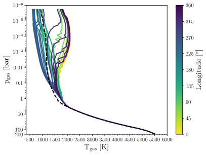
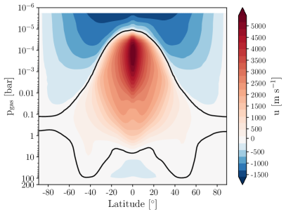
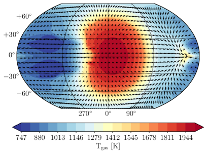
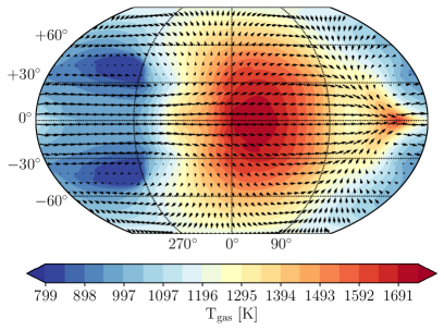
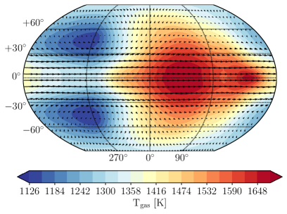
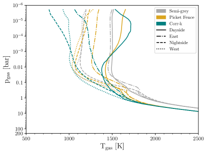
We present results using Exo-FMS coupled to the real gas correlated-k model. Due to the significant computational cost, the simulation is performed for 1600 days, with the final 100 day average taken as the presented results. The simulation is initialised according to scheme outlined in Sect. 3. For the input correlated-k opacities we use the pre-mixed tables with equilibrium condensation as outlined in Sect. 2.5. Figure 5 shows the results of our coupled GCM and correlated-k scheme.

As seen in Fig. 5 our T-p profiles show fluctuations in some dayside profiles at upper atmospheric regions. This can attributed to the condensation of TiO and VO which happens near the T-p of the fluctuations leading to strong gradients in the VMR of gas phase TiO and VO across this T-p range. An additional explanation is possibly related to numerical errors when interpolating the pre-mixed k-table T-p points to the local atmospheric T-p as discussed in Amundsen et al. (2017). This artefact can possibly be improved upon by increasing the k-table resolution near the temperatures important for TiO and VO condensation, making a pre-mixed k-table without TiO and VO included (commonly used in the literature e.g. Amundsen et al. (2016); Kataria et al. (2016)), or using a random overlap scheme (Amundsen et al., 2017).

5.4 HD 209458b-like comparisons

Figure 6: Mean T-p profile comparisons between the semi-grey, picket fence and corr-k HD 209458b-like simulations. Dayside, nightside, eastern terminator and western terminator mean T-p profiles are plotted in solid, dash-dot, dashed and dotted line styles respectively.

The correlated-k and picket fence scheme produce very similar zonal mean velocity structures and absolute values. The temperature maps are also similar across the 10^-4-1 bar range. Differences are mostly seen in the upper atmospheric temperatures at low pressure ($\lesssim$ 10^-4 bar), where the 30 correlated-k bands are able to more efficiently cool the atmosphere compared to the two band picket fence scheme. The upper atmospheric temperature inversion and maximum temperature due to TiO and VO opacities are also well reproduced by the picket fence scheme. Since the radiative-timescales are short at these low pressures, these differences are most likely a direct result of the RT scheme used, rather than any dynamical effect.

Due to the added computational burden when performing correlated-k models, our chosen end points between the correlated-k, picket fence/semi-grey runs were different (1600 and 3600 days respectively). We have checked the daily output of the non-grey and semi-grey models at 1600 days, which shows a small difference (at most $\lesssim$ 5$\%$, within the natural variability of the model) in the T-p profiles, lat-lon maps and zonal mean velocities from the 100 day average at 3600 days. This suggests that the extra 2000 days runtime in the non-grey and semi-grey models does not affect the outcome of the post-processing much, and the comparison to the corr-k output is still reasonable to perform.

The semi-grey model produces a different upper atmospheric temperature structure compared to the correlated-k model, with temperature patterns in the at pressures $<$ 10^-1 bar appearing notably different. The central jet is also more extended in latitude compared to the picket fence and correlated-k models.

In Fig. 6 we compare the average dayside, nightside and east and west terminator regions from each HD 209458b simulation. It is clear that the correlated-k and picket fence model are similar, especially in the higher pressure regions. Also evident is the different deep adiabatic gradient between the semi-grey model and the picket fence and corr-k models. This is probably due to assuming a too strong exponent term scaling in the semi-grey optical depth parameters. It is likely the pressure dependent semi-grey parameters could be adjusted to fit the adiabatic region produced in the corr-k model better, however, it is not clear how to set these parameters on a case by base basis without first comparing directly to the corr-k or picket fence model results.

In comparison to previous studies, we are able to reproduce qualitatively well the HD 209458b simulations performed in (Showman et al., 2009), with a similar range of temperature and pressures with depth and lat-lon pressure level maps. Significant differences in the deep T-p structures are due to a lower internal temperature used in Showman et al. (2009) and different initial condition assumptions used in this study. Our results are less compatible with the simulations performed Kataria et al. (2016) and Amundsen et al. (2016) due to our inclusion of TiO and VO opacities which greatly affect the dayside T-p profiles. However, our nightside profiles show good agreement with the results of Kataria et al. (2016) and Amundsen et al. (2016), suggesting our correlated-k scheme is producing comparable results to other well used models.

6 Post-processing

Figure 7: Transmission and dayside emission spectra post-processing of the HD 209458b simulations. For the transmission spectra, the Sing et al. (2016) (grey points), Evans et al. (2015) (gold squares) and Crossfield et al. (2012) (teal diamond) observations are over-plotted for comparison. For the dayside emission spectra, the Line et al. (2016) (grey points), Evans et al. (2015) (gold squares) and Crossfield et al. (2012) (teal diamond) observations are also plotted.

Figure 8: Phase curves for Spitzer IRAC and MIPS bands post-processing of the HD 209458b simulations. The dayside emission values from Evans et al. (2015) and Crossfield et al. (2012) are plotted at 0.5 phase.

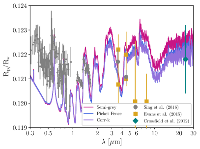
In this section we post-process our HD209458b-like simulations and compare the results to available observational data. We use the CMCRT code of Lee et al. (2017) in correlated-k mode (Lee et al., 2019). For CMCRT input opacities we use nemesis (Irwin et al., 2008) formatted k-tables available from the ExoMolOP database (Chubb et al., 2021). Table 1 shows the opacity sources and references used for the post-processing.

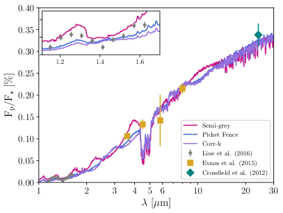
Figure 7 presents the transmission and dayside emission spectra. For the transmission spectra, the correlated-k model was scaled to the $\approx$1.4 $\mu$m H₂O feature and the picket fence and grey gas results scaled to the Rayleigh scattering slope of the real gas model. From the transmission spectra figure it is clear that the picket fence and corr-k model produce highly similar transmission spectra. Our semi-grey model produces larger molecular features, probably due to the increased scale height due it’s generally higher atmospheric temperatures. In emission, again the picket fence and corr-k model agree well across the whole wavelength range, with the most difference occurring around the 4$\mu$m range.

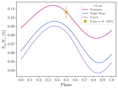
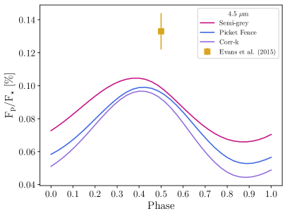
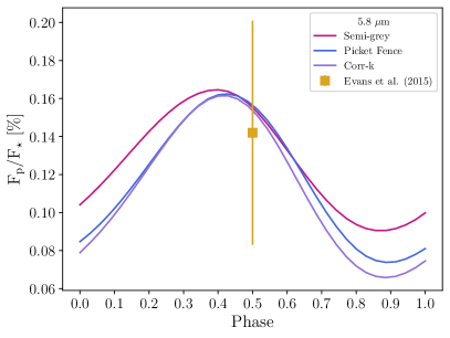
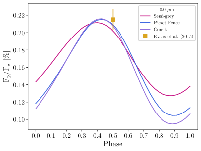
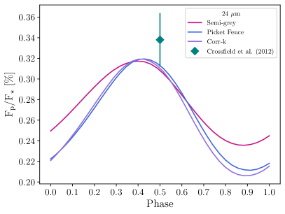
Figure 8 presents a comparison of the Spitzer bandpass phase curves predictions between the models. From these results it is clear the picket fence scheme reproduces well the correlated-k model results, with good agreement for the maximum flux shift and day-night contrast. However, the picket fence scheme has more difficulty reproducing the nightside fluxes of the corr-k model, where the cooling of the upper atmosphere is more important in controlling the T-p structure.

7 Discussion

Figure 9: $\gamma_{P}$ = $\kappa_{P}$/$\kappa_{R}$ calculated from the solar metallicity Freedman et al. (2014) tables. Coloured lines denote the gas pressure in bar. The black lines show the Parmentier et al. (2015) expression as a function of T_eff (solid: with TiO/VO, dashed: w/o TiO/VO). The dotted grey line shows the grey region where $\kappa_{P}$ = $\kappa_{R}$.

Our picket fence scheme following Parmentier & Guillot (2014) and Parmentier et al. (2015) shows promise in improving the realism of the RT calculations with simple modifications to current semi-grey RT schemes. Our initial modelling was able to produce good agreement with the dayside temperature profiles of real gas model. We caution a more quantitive agreement will require a more careful choice with respect to the best parameterisations with this scheme. Furthermore, our test was not a fair one-to-one comparison due to several factors:

• Different opacity sources between the correlated-k scheme and Rosseland mean Freedman et al. (2014) studies.

• Different gas phase abundances through the choice of solar elemental ratio reference, different CE solver and equilibrium condensation data used between Freedman et al. (2014) and Woitke et al. (2018).

As seen in our GCM results and also discussed in 1D models of Parmentier et al. (2015), the most difference between the picket fence and real gas models occurs in the upper atmosphere from p_gas $\lesssim$ 10^-3 bar. This is due the picket fence scheme not actively capturing efficient cooling that occurs in these less dense regions, as extensively proven in Parmentier & Guillot (2014); Parmentier et al. (2015).

However, given the simplicity of implementing a picket fence scheme, this offers a useful ‘middle-ground’ in physical realism between the semi-grey and real gas RT schemes. This scheme has potential to be further generalised with the inclusion of shortwave and longwave scattering components (e.g. Pierrehumbert, 2010; Mohandas et al., 2018), enabling the simulation of radiative feedback due to cloud formation. Including radiative feedback from non-equilibrium chemistry may be more difficult to include in the current picket fence framework, since the Rosseland mean tables from Freedman et al. (2014) use chemical equilibrium results. A more generalised scheme would be required to take varying volume mixing ratios into account. A potential hybrid approach may be to evolve simulations for an extended ‘spin-up’ period using the picket fence scheme, switching to the correlated-k scheme for the latter half of the simulation when adding additional feedback mechanisms.

Our current simulations are not representative of a fully converged simulation due to long radiative-timescales and mixing timescales (10000+ days) in the lower atmosphere, examined by recent studies (e.g. Mayne et al., 2017; Wang & Wordsworth, 2020). We note that a long integration time on the scale of Wang & Wordsworth (2020) is unfeasible for scope of this study. Despite this limitation of the current study, the proposed picket fence scheme offers an efficient and more realistic RT solution than semi-grey schemes for longer integration investigations to study deep layer radiative and momentum transport in the atmosphere.

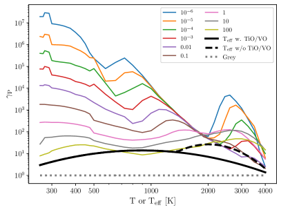
The ‘greyness’ of the wavelength dependent opacity structure can be inferred by the ratio of the Planck mean to Rosseland mean (e.g. Guillot, 2010)

$$\gamma_{P}=\frac{\kappa_{P}}{\kappa_{R}},$$ (21)

where if $\gamma_{P}$ = 1, the atmospheric opacity is grey with $\gamma_{P}$ $\gg$ 1 characteristic of a non-grey atmosphere. In Fig. 9 we show $\gamma_{P}$ as given by the Planck and Rosseland mean, solar metallicity opacity tables presented in Freedman et al. (2014). This shows that generally the non-greyness of an atmosphere increases with decreasing temperature and pressure, typical environments important for the atmospheric cooling efficiency. In addition, we show the $\gamma_{P}$ expression from Parmentier et al. (2015) with and without TiO and VO opacity included. This shows that the relationships between the parameters in Parmentier et al. (2015) is vital to accurate determination of the visible band and picket fence opacity ratios for the column, since putting directly the local $\gamma_{P}$ from the Freedman et al. (2014) tables into the framework would probably not result in fitting the correlated-k T-p profiles well.

8 Summary & Conclusions

In this study we successfully benchmarked the Exo-FMS GCM model to contemporary studies of hot gas giant model atmospheres. Using the semi-grey scheme, we were able to reproduce qualitatively and quantitatively the results of the Heng et al. (2011b) study, but only compared qualitatively with the Rauscher & Menou (2012) results. We coupled a real gas, correlated-k scheme to Exo-FMS, and were able to match well with the general behaviour of Showman et al. (2009), although with differences in the detailed results.

We propose a general initial condition scheme using the analytical radiative-equilibrium profiles from Parmentier & Guillot (2014); Parmentier et al. (2015) at the sub-stellar point. This offers a simple way to practically implement recent recommendations by Sainsbury-Martinez et al. (2019) and internal temperature considerations in Thorngren et al. (2019).

We implemented a non-grey picket fence RT scheme (Parmentier & Guillot, 2014; Parmentier et al., 2015) in the GCM and compared the results of the semi-grey, picket fence and real gas RT schemes on a HD 209458b-like simulation set-up. The picket fence scheme was able to reproduce well the global and local T-p profiles of the real gas model at pressures most responsible to the observable characteristics of the atmosphere. The picket fence model produces highly comparable transmission and emission spectra to the corr-k model when post-processed. The phase curve properties of the picket fence model are also very comparable to the corr-k results, with the most differences occurring on the nightside regions of the planet.

Overall, we suggest that the picket fence approach offers a potentially efficient way to significantly improve the realism of the radiative-transfer characteristics in hot Jupiter GCMs, avoiding use of computationally expensive real gas calculations. We suggest that the implementation of such schemes will be highly useful for future GCM modelling that require longer integration times or experiments with parameter examinations that wish to retain a more realistic RT solution, or are interested in producing computationally cheaper GCM results while retaining the transmission, emission and phase curve characteristics of the atmosphere given by the more expensive RT schemes.

Data and code availability

1D column versions that emulate the FMS GCM of the semi-grey, picket fence schemes and correlated-k approach are available from the lead author’s GitHub: https://github.com/ELeeAstro These include our initial condition module and dry convective adjustment scheme. GCM model output in NetCDF format is available from Zendoo, DOI: 10.5281/zenodo.5011921 . All other data and code is available from the authors on a collaborative basis.

Appendix A RT scheme validation

Figure 10: Validation of the semi-grey RT set-up following Parmentier et al. (2015). Left: The analytical self-luminous solution of Chandrasekhar (1960) (T_a) is compared to the numerical solution (T_n). Right: Semi-grey analytical T-p solution from of Guillot (2010) (T_a - T_irr = 1288 K, T_int = 500 K, $\mu_{\star}$ = 1/$\sqrt{3}$, $\gamma_{\rm v}$ = 0.25) compared to the numerical solution (T_n). In each case, we also compare to the 5 Gaussian quadrature points solution used in Parmentier et al. (2015) (P15), showing our 2 points give similar $\%$ error to the 5 point case.

Figure 11: Validation of the semi-grey and corr-k RT set-up. Left: The analytical T-p (T_a - T_irr = 1288 K, T_int = 500 K, $\mu_{\star}$ = 1/$\sqrt{3}$), following the analytical profile of Parmentier et al. (2015) and the equivalent numerical set-up. Right: The correlated-k model instantaneous heating rates, following the Test 2 T-p profile in Amundsen et al. (2014) with the scheme used in the GCM.

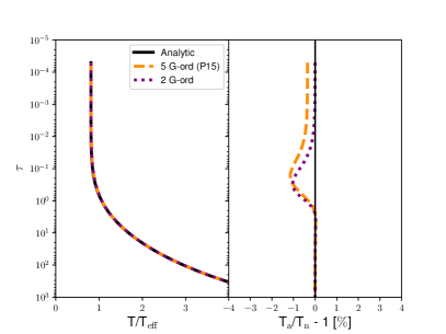
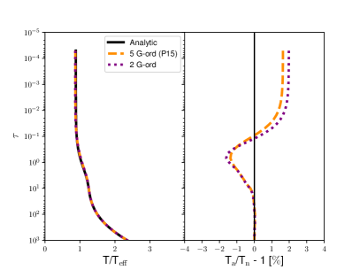
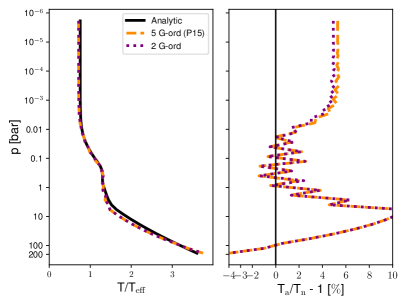
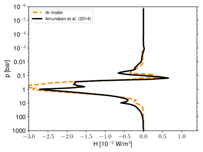
In this appendix we validate the radiative-transfer scheme used in this study. Figure 10 shows a comparison between the Chandrasekhar (1960) analytic solution for a self-luminous atmosphere and a repeat of the Parmentier et al. (2015) for a Guillot (2010) analytical semi-grey profile. This shows our scheme produces excellent agreement to within 2 $\%$ of the analytical solutions. Figure 11 shows a comparison with the picket fence scheme, showing good agreement with the analytical solution, to within 5$\%$ in the radiative region and 10$\%$ in the deeper convective region. We also show heating rates from Test 2 in Amundsen et al. (2014), showing excellent agreement for the correlated-k scheme to contemporary models. Differences can most probably be attributed to the use of different line-list opacities between Amundsen et al. (2014) and this study, and differences between the analytic Burrows & Sharp (1999) CE abundances used in Amundsen et al. (2014) and the numerical CE solver Woitke et al. (2018) used in this study.

Appendix B GCM simulation parameters

Table 2: Adopted GCM simulation parameters for the HD 209458b-like semi-grey (Sect. 5.1), non-grey (Sect. 5.2) and correlated-k (Sect. 5.3) simulations. Bulk parameters are derived from the values found in the exoplanet.eu database.

Symbol	semi-grey	non-grey	corr-k	Unit	Description
Tirr	2091	2091	spectral	K	Irradiation temperature
AB	0	$\star$	0	-	Bond albedo ($\star$ Parmentier et al., 2015)
Tint	571	571	571	K	Internal temperature (Thorngren et al., 2019)
P0	220	220	220	bar	Reference surface pressure
$\kappa_{V}$	6.13$\cdot$10-4	$\star$ 3 bands	30 bands	m2g-1	Visible band opacity ($\star$ Parmentier et al., 2015)
$\kappa_{IR}$	1$\cdot$10-3	$\star$ 2 bands	30 bands	m2g-1	Infrared band opacity ($\star$ Parmentier et al., 2015)
nL	2	-	-	-	IR power-law index
fl	0.0005	-	-	-	IR linear component fraction (Heng et al., 2011b)
cp	1.3$\cdot$104	1.3$\cdot$104	1.3$\cdot$104	J K-1 kg-1	Specific heat capacity
R	3556.8	3556.8	3556.8	J K-1 kg-1	Ideal gas constant
$\kappa$	0.2736	0.2736	0.2736	J K-1 kg-1	Adiabatic coefficient
gHJ	8.98	8.98	8.98	m s-2	Acceleration from gravity
RHJ	9.865$\cdot$107	9.865$\cdot$107	9.865$\cdot$107	m	Radius of HJ
$\Omega_{\rm HJ}$	2.063$\cdot$10-5	2.063$\cdot$10-5	2.063$\cdot$10-5	rad s-1	Rotation rate of HJ
$\Delta$thydo	30	30	20	s	Hydrodynamic time-step
$\Delta$trad	30	30	100	s	Radiaitve time-step
Nv	53	53	53	-	Vertical level resolution
d2	0.02	0.02	0.02	-	div. dampening coefficient

Appendix C Unbiased Monte Carlo RT transmission sampling

In Lee et al. (2019) a transmission spectra mode in CMCRT was presented which was found to produce a biasing in the results due to binning of photon packets into discrete transmission limb impact parameters inside a spherical geometrical grid. This led to a biasing towards higher optical depths, resulting in slightly higher R_p/R_⋆ at the 10s ppm level compared to the benchmark cases. Here we present a simple unbiased Monte Carlo sampling method for producing transmission spectra from GCM output.

The transmission spectra equation is given by (e.g. Dobbs-Dixon & Agol, 2013; Robinson, 2017)

$$\left(\frac{R_{p,\lambda}}{R_{\star}}\right)^{2}=\frac{1}{R_{\star}^{2}}\left(R_{p,0}^{2}+2\int_{R_{p,0}}^{\infty}[1-\mathcal{T}(b)]bdb\right),$$ (22)

where R_p,λ [m] is the wavelength dependent radius of the planet, R_⋆ [m] the radius of the host star, R_p,0 [m] the bulk planetary disk radius, $\mathcal{T}$ the transmission function, and $b$ [m] the impact parameter. Formally the upper limit for the integral in Eq. 22 is $\infty$. This is replaced by the top of atmosphere radius, R_p,TOA [m], as per the simulation output to facilitate numerical calculations.

Following the principles of integration through independent sampling, the result of the integral in Eq. 22, I_p, is approximated by simulating a suitably large number of N_ph photon packets that sample the integral function

$$\langle I_{p}\rangle=\frac{(R_{p,TOA}-R_{p,0})}{N_{ph}}\sum^{N_{ph}}_{i}[1-e^{-\tau_{i}}]b_{i},$$ (23)

where $\tau_{i}$ is the optical depth that the packet requires to escape the atmosphere toward the observational direction at impact parameter b_i. The scheme therefore reduces to sampling a random impact parameter, b_i, between R_p,TOA and R_p,0 at randomly chosen transmission annulus for the photon packet. The optical depths and impact parameter of each packet is then tracked and summed during the simulation, before normalisation at the end of the simulation. In our testing, this scheme avoids the geometrical biasing found in Lee et al. (2019) at the cost of additional packet noise, requiring more packets ($\approx$10$\times$) to be simulated to reach a similar level of noise to the previous method.

We note this method is not limited to MCRT models but can be utilised by 1D/3D ray tracing codes to avoid manually choosing the initial start position of the optical depth tracing, this is the case for the Lee et al. (2019) which is a hybrid MCRT and ray tracing model.

References

- Allard et al. (2011) Allard F., Homeier D., Freytag B., 2011, in Johns-Krull C., Browning M. K., West A. A., eds, Astronomical Society of the Pacific Conference Series Vol. 448, 16th Cambridge Workshop on Cool Stars, Stellar Systems, and the Sun. p. 91 (arXiv:1011.5405)
- Amundsen et al. (2014) Amundsen D. S., Baraffe I., Tremblin P., Manners J., Hayek W., Mayne N. J., Acreman D. M., 2014, A&A, 564, A59
- Amundsen et al. (2016) Amundsen D. S., et al., 2016, A&A, 595, A36
- Amundsen et al. (2017) Amundsen D. S., Tremblin P., Manners J., Baraffe I., Mayne N. J., 2017, A&A, 598, A97
- Asplund et al. (2009) Asplund M., Grevesse N., Sauval A. J., Scott P., 2009, ARA&A, 47, 481
- Azzam et al. (2016) Azzam A. A. A., Tennyson J., Yurchenko S. N., Naumenko O. V., 2016, MNRAS, 460, 4063
- Barber et al. (2014) Barber R. J., Strange J. K., Hill C., Polyansky O. L., Mellau G. C., Yurchenko S. N., Tennyson J., 2014, MNRAS, 437, 1828
- Barstow et al. (2014) Barstow J. K., Aigrain S., Irwin P. G. J., Hackler T., Fletcher L. N., Lee J. M., Gibson N. P., 2014, ApJ, 786, 154
- Barton et al. (2013) Barton E. J., Yurchenko S. N., Tennyson J., 2013, MNRAS, 434, 1469
- Batalha et al. (2019) Batalha N. E., Marley M. S., Lewis N. K., Fortney J. J., 2019, ApJ, 878, 70
- Bean et al. (2018) Bean J. L., et al., 2018, PASP, 130, 114402
- Beltz et al. (2021) Beltz H., Rauscher E., Brogi M., Kempton E. M. R., 2021, AJ, 161, 1
- Bernath (2020) Bernath P. F., 2020, Journal of Quantitative Spectroscopy and Radiative Transfer, 240, 106687
- Blecic et al. (2017) Blecic J., Dobbs-Dixon I., Greene T., 2017, ApJ, 848, 127
- Bourrier et al. (2020) Bourrier V., et al., 2020, A&A, 637, A36
- Broeg et al. (2013) Broeg C., et al., 2013, in European Physical Journal Web of Conferences. p. 03005 (arXiv:1305.2270), doi:10.1051/epjconf/20134703005
- Burrows & Sharp (1999) Burrows A., Sharp C. M., 1999, ApJ, 512, 843
- Cahoy et al. (2010) Cahoy K. L., Marley M. S., Fortney J. J., 2010, ApJ, 724, 189
- Caldas et al. (2019) Caldas A., Leconte J., Selsis F., Waldmann I. P., Bordé P., Rocchetto M., Charnay B., 2019, A&A, 623, A161
- Carone et al. (2020) Carone L., et al., 2020, MNRAS, 496, 3582
- Chandrasekhar (1935) Chandrasekhar S., 1935, MNRAS, 96, 21
- Chandrasekhar (1960) Chandrasekhar S., 1960, Radiative transfer
- Charnay et al. (2015) Charnay B., Meadows V., Leconte J., 2015, ApJ, 813, 15
- Charnay et al. (2021) Charnay B., et al., 2021, Experimental Astronomy,
- Chubb et al. (2020) Chubb K. L., Tennyson J., Yurchenko S. N., 2020, MNRAS, 493, 1531
- Chubb et al. (2021) Chubb K. L., et al., 2021, A&A, 646, A21
- Coles et al. (2019) Coles P. A., Yurchenko S. N., Tennyson J., 2019, MNRAS, 490, 4638
- Crossfield et al. (2012) Crossfield I. J. M., Knutson H., Fortney J., Showman A. P., Cowan N. B., Deming D., 2012, ApJ, 752, 81
- Dalgarno & Williams (1962) Dalgarno A., Williams D. A., 1962, ApJ, 136, 690
- Daylan et al. (2021) Daylan T., et al., 2021, AJ, 161, 131
- Ding & Wordsworth (2019) Ding F., Wordsworth R. D., 2019, ApJ, 878, 117
- Dobbs-Dixon & Agol (2013) Dobbs-Dixon I., Agol E., 2013, MNRAS, 435, 3159
- Dobbs-Dixon & Cowan (2017) Dobbs-Dixon I., Cowan N. B., 2017, ApJL, 851, L26
- Ehrenreich et al. (2020) Ehrenreich D., et al., 2020, Nature, 580, 597
- Evans et al. (2015) Evans T. M., Aigrain S., Gibson N., Barstow J. K., Amundsen D. S., Tremblin P., Mourier P., 2015, MNRAS, 451, 680
- Feng et al. (2016) Feng Y. K., Line M. R., Fortney J. J., Stevenson K. B., Bean J., Kreidberg L., Parmentier V., 2016, ApJ, 829, 52
- Flowers et al. (2019) Flowers E., Brogi M., Rauscher E., Kempton E. M. R., Chiavassa A., 2019, AJ, 157, 209
- Fortney et al. (2005) Fortney J. J., Marley M. S., Lodders K., Saumon D., Freedman R., 2005, ApJL, 627, L69
- Freedman et al. (2014) Freedman R. S., Lustig-Yaeger J., Fortney J. J., Lupu R. E., Marley M. S., Lodders K., 2014, The Astrophysical Journal Supplement Series, 214, 25
- Garcia Munoz & Isaak (2015) Garcia Munoz A., Isaak K. G., 2015, Proceedings of the National Academy of Science, 112, 13461
- GharibNezhad et al. (2013) GharibNezhad E., Shayesteh A., Bernath P. F., 2013, MNRAS, 432, 2043
- Gordon et al. (2017) Gordon I., et al., 2017, Journal of Quantitative Spectroscopy and Radiative Transfer, 203, 3
- Grimm & Heng (2015) Grimm S. L., Heng K., 2015, ApJ, 808, 182
- Grimm et al. (2021) Grimm S. L., et al., 2021, ApJS, 253, 30
- Guillot (2010) Guillot T., 2010, A&A, 520, A27
- Hammond & Pierrehumbert (2017) Hammond M., Pierrehumbert R. T., 2017, ApJ, 849, 152
- Hammond & Pierrehumbert (2018) Hammond M., Pierrehumbert R. T., 2018, ApJ, 869, 65
- Harris et al. (2006) Harris G. J., Tennyson J., Kaminsky B. M., Pavlenko Y. V., Jones H. R. A., 2006, MNRAS, 367, 400
- Heng (2017) Heng K., 2017, Exoplanetary Atmospheres: Theoretical Concepts and Foundations
- Heng & Showman (2015) Heng K., Showman A. P., 2015, Annual Review of Earth and Planetary Sciences, 43, 509
- Heng et al. (2011a) Heng K., Menou K., Phillipps P. J., 2011a, MNRAS, 413, 2380
- Heng et al. (2011b) Heng K., Frierson D. M. W., Phillipps P. J., 2011b, MNRAS, 418, 2669
- Heng et al. (2014) Heng K., Mendonça J. M., Lee J.-M., 2014, ApJS, 215, 4
- Heng et al. (2018) Heng K., Malik M., Kitzmann D., 2018, ApJS, 237, 29
- Holton & Hakim (2013) Holton J. R., Hakim G. J., 2013, An introduction to dynamic meteorology, 5th. edn. Elsevier, Amsterdam
- Hunter (2007) Hunter J. D., 2007, Computing In Science & Engineering, 9, 90
- Irwin et al. (2008) Irwin P. G. J., et al., 2008, Journal of Quantitative Spectroscopy and Radiative Transfer, 109, 1136
- Irwin et al. (2020) Irwin P. G. J., Parmentier V., Taylor J., Barstow J., Aigrain S., Lee E. K. H., Garland R., 2020, MNRAS, 493, 106
- Jansen & Kipping (2020) Jansen T., Kipping D., 2020, MNRAS, 494, 4077
- John (1988) John T. L., 1988, A&A, 193, 189
- Jones et al. (2001) Jones E., Oliphant T., Peterson P., et al., 2001, SciPy: Open source scientific tools for Python, http://www.scipy.org/
- Karman et al. (2019) Karman T., et al., 2019, Icarus, 328, 160
- Kataria et al. (2013) Kataria T., Showman A. P., Lewis N. K., Fortney J. J., Marley M. S., Freedman R. S., 2013, ApJ, 767, 76
- Kataria et al. (2014) Kataria T., Showman A. P., Fortney J. J., Marley M. S., Freedman R. S., 2014, ApJ, 785, 92
- Kataria et al. (2016) Kataria T., Sing D. K., Lewis N. K., Visscher C., Showman A. P., Fortney J. J., Marley M. S., 2016, ApJ, 821, 9
- Kitzmann et al. (2020) Kitzmann D., Heng K., Oreshenko M., Grimm S. L., Apai D., Bowler B. P., Burgasser A. J., Marley M. S., 2020, ApJ, 890, 174
- Komacek & Showman (2016) Komacek T. D., Showman A. P., 2016, ApJ, 821, 16
- Komacek et al. (2017) Komacek T. D., Showman A. P., Tan X., 2017, ApJ, 835, 198
- Kramida et al. (2013) Kramida A., Ralchenko Y., Reader J., 2013, NIST Atomic Spectra Database – Version 5
- Kuroda et al. (2014) Kuroda T., Medvedev A. S., Hartogh P., 2014, Icarus, 242, 149
- Kurucz (1970) Kurucz R. L., 1970, SAO Special Report, 309
- Kurucz & Bell (1995) Kurucz R. L., Bell B., 1995, Atomic line list
- Lacis & Oinas (1991) Lacis A. A., Oinas V., 1991, J. Geophys. Res., 96, 9027
- Lebonnois et al. (2010) Lebonnois S., Hourdin F., Eymet V., Crespin A., Fournier R., Forget F., 2010, Journal of Geophysical Research: Planets, 115
- Lee & Richardson (2012) Lee C., Richardson M., 2012, Icarus, 221, 1173
- Lee et al. (2017) Lee E. K. H., Wood K., Dobbs-Dixon I., Rice A., Helling C., 2017, A&A, 601
- Lee et al. (2019) Lee E. K. H., Taylor J., Grimm S. L., Baudino J.-L., Garland R., Irwin P. G. J., Wood K., 2019, MNRAS, 487, 2082
- Lee et al. (2020) Lee E. K. H., Casewell S. L., Chubb K. L., Hammond M., Tan X., Tsai S.-M., Pierrehumbert R. T., 2020, MNRAS, 496, 4674
- Li et al. (2015) Li G., Gordon I. E., Rothman L. S., Tan Y., Hu S.-M., Kassi S., Campargue A., Medvedev E. S., 2015, The Astrophysical Journal Supplement Series, 216, 15
- Li et al. (2018) Li C., Le T., Zhang X., Yung Y. L., 2018, J. Quant. Spectrosc. Radiative Transfer, 217, 353
- Limaye et al. (2018) Limaye S. S., Grassi D., Mahieux A., Migliorini A., Tellmann S., Titov D., 2018, Space Sci. Rev., 214, 102
- Lin (2004) Lin S.-J., 2004, Monthly Weather Review, 132, 2293
- Line et al. (2016) Line M. R., et al., 2016, AJ, 152, 203
- Mayne et al. (2014) Mayne N. J., et al., 2014, A&A, 561, A1
- Mayne et al. (2017) Mayne N. J., et al., 2017, A&A, 604, A79
- Mayne et al. (2019) Mayne N. J., Drummond B., Debras F., Jaupart E., Manners J., Boutle I. A., Baraffe I., Kohary K., 2019, ApJ, 871, 56
- Mayorga et al. (2019) Mayorga L. C., Batalha N. E., Lewis N. K., Marley M. S., 2019, AJ, 158, 66
- McKemmish et al. (2016) McKemmish L. K., Yurchenko S. N., Tennyson J., 2016, MNRAS, 463, 771
- McKemmish et al. (2019) McKemmish L. K., Masseron T., Hoeijmakers H. J., Pérez-Mesa V., Grimm S. L., Yurchenko S. N., Tennyson J., 2019, MNRAS, 488, 2836
- Mendonça (2020) Mendonça J. M., 2020, MNRAS, 491, 1456
- Mendonça et al. (2015) Mendonça J. M., Read P. L., Wilson C. F., Lee C., 2015, Planet. Space Sci., 105, 80
- Mendonça et al. (2016) Mendonça J. M., Grimm S. L., Grosheintz L., Heng K., 2016, ApJ, 829, 115
- Mendonça et al. (2018) Mendonça J. M., Malik M., Demory B.-O., Heng K., 2018, AJ, 155, 150
- Mendonça & Read (2016) Mendonça J., Read P., 2016, Planetary and Space Science, 134, 1
- Merritt et al. (2020) Merritt S. R., et al., 2020, A&A, 636, A117
- Miller-Ricci Kempton & Rauscher (2012) Miller-Ricci Kempton E., Rauscher E., 2012, ApJ, 751, 117
- Mohandas et al. (2018) Mohandas G., Pessah M. E., Heng K., 2018, ApJ, 858, 1
- Nagler et al. (2019) Nagler P. C., et al., 2019, Journal of Astronomical Instrumentation, 8, 1950011
- Oreshenko et al. (2016) Oreshenko M., Heng K., Demory B.-O., 2016, MNRAS, 457, 3420
- Parmentier & Guillot (2014) Parmentier V., Guillot T., 2014, A&A, 562, A133
- Parmentier et al. (2015) Parmentier V., Guillot T., Fortney J. J., Marley M. S., 2015, A&A, 574, A35
- Parmentier et al. (2016) Parmentier V., Fortney J. J., Showman A. P., Morley C., Marley M. S., 2016, ApJ, 828, 22
- Parmentier et al. (2021) Parmentier V., Showman A. P., Fortney J. J., 2021, MNRAS, 501, 78
- Pierrehumbert (2010) Pierrehumbert R. T., 2010, Principles of Planetary Climate
- Pierrehumbert & Ding (2016) Pierrehumbert R. T., Ding F., 2016, Proceedings of the Royal Society of London Series A, 472, 20160107
- Pino et al. (2020) Pino L., et al., 2020, ApJL, 894, L27
- Polichtchouk et al. (2014) Polichtchouk I., Cho J. Y. K., Watkins C., Thrastarson H. T., Umurhan O. M., de la Torre Juárez M., 2014, Icarus, 229, 355
- Polyansky et al. (2018) Polyansky O. L., Kyuberis A. A., Zobov N. F., Tennyson J., Yurchenko S. N., Lodi L., 2018, MNRAS, 480, 2597
- Rauscher & Menou (2010) Rauscher E., Menou K., 2010, ApJ, 714, 1334
- Rauscher & Menou (2012) Rauscher E., Menou K., 2012, ApJ, 750, 96
- Ricker et al. (2014) Ricker G. R., et al., 2014, in Space Telescopes and Instrumentation 2014: Optical, Infrared, and Millimeter Wave. p. 914320 (arXiv:1406.0151), doi:10.1117/12.2063489
- Robinson (2017) Robinson T. D., 2017, ApJ, 836, 236
- Rothman et al. (2010) Rothman L. S., et al., 2010, J. Quant. Spectrosc. Radiative Transfer, 111, 2139
- STScI Development Team (2013) STScI Development Team 2013, pysynphot: Synthetic photometry software package (ascl:1303.023)
- Sainsbury-Martinez et al. (2019) Sainsbury-Martinez F., et al., 2019, A&A, 632, A114
- Schneider & Liu (2009) Schneider T., Liu J., 01 Mar. 2009, Journal of the Atmospheric Sciences, 66, 579
- Seidel et al. (2019) Seidel J. V., et al., 2019, A&A, 623, A166
- Showman et al. (2008) Showman A. P., Cooper C. S., Fortney J. J., Marley M. S., 2008, ApJ, 682, 559
- Showman et al. (2009) Showman A. P., Fortney J. J., Lian Y., Marley M. S., Freedman R. S., Knutson H. A., Charbonneau D., 2009, ApJ, 699, 564
- Showman et al. (2020) Showman A. P., Tan X., Parmentier V., 2020, Space Sci. Rev., 216, 139
- Shporer et al. (2019) Shporer A., et al., 2019, AJ, 157, 178
- Sing et al. (2016) Sing D. K., et al., 2016, Nature, 529, 59
- Sousa-Silva et al. (2015) Sousa-Silva C., Al-Refaie A. F., Tennyson J., Yurchenko S. N., 2015, MNRAS, 446, 2337
- Tan & Komacek (2019) Tan X., Komacek T. D., 2019, ApJ, 886, 26
- Tan & Showman (2020) Tan X., Showman A. P., 2020, ApJ, 902, 27
- Taylor et al. (2020) Taylor J., Parmentier V., Irwin P. G. J., Aigrain S., Lee E. K. H., Krissansen-Totton J., 2020, arXiv e-prints, p. arXiv:2002.00773
- Thalman et al. (2014) Thalman R., Zarzana K. J., Tolbert M. A., Volkamer R., 2014, J. Quant. Spectrosc. Radiative Transfer, 147, 171
- The Astropy Collaboration et al. (2018) The Astropy Collaboration et al., 2018, preprint, (arXiv:1801.02634)
- Thomson & Vallis (2019) Thomson S. I., Vallis G. K., 2019, Atmosphere, 10, 803
- Thorngren et al. (2019) Thorngren D., Gao P., Fortney J. J., 2019, ApJL, 884, L6
- Tinetti et al. (2016) Tinetti G., et al., 2016, in Space Telescopes and Instrumentation 2016: Optical, Infrared, and Millimeter Wave. p. 99041X, doi:10.1117/12.2232370
- Toon et al. (1989) Toon O. B., McKay C. P., Ackerman T. P., Santhanam K., 1989, J. Geophys. Res., 94, 16287
- Venot et al. (2020) Venot O., et al., 2020, ApJ, 890, 176
- Wang & Wordsworth (2020) Wang H., Wordsworth R., 2020, ApJ, 891, 7
- Woitke et al. (2018) Woitke P., Helling C., Hunter G. H., Millard J. D., Turner G. E., Worters M., Blecic J., Stock J. W., 2018, A&A, 614, A1
- Wong et al. (2020a) Wong I., et al., 2020a, AJ, 159, 104
- Wong et al. (2020b) Wong I., et al., 2020b, AJ, 160, 88
- Young et al. (2019) Young R. M., Read P. L., Wang Y., 2019, Icarus, 326, 225
- Yurchenko et al. (2017) Yurchenko S. N., Amundsen D. S., Tennyson J., Waldmann I. P., 2017, A&A, 605, A95