(cvpr) Package cvpr Warning: Single column document - CVPR requires papers to have two-column layout. Please load document class ‘article’ with ‘twocolumn’ option
Supplementary Materials for
NCIS: Neural Contextual Iterative Smoothing for
Purifying Adversarial Perturbations
1 Additional Analysis for Adversarial Noise
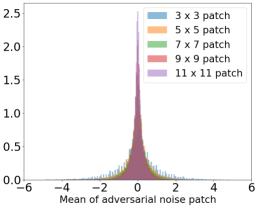
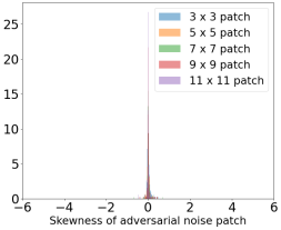
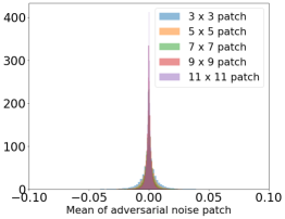
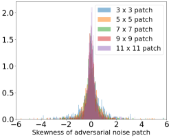
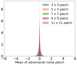
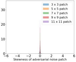
Figure 1, 2, and 3 show additional experimental results of adversarial noise. We conducted the experiments on the same dataset used in Section 3.2 of the manuscript but with different attack methods. Figure 1 is the result of targeted PGD [12] attack with the same , and attack iterations proposed in Section 3.2 of the manuscript. Figure 2 shows analysis of untargeted PGD attack with and Figure 3 is about CW [5] attack with 10 attack iterations. From all the experimental results, we observe that the patches of adversarial noises generated from untargeted / targeted and / optimization-based adversarial attacks consistently show more or less zero mean and have symmetric distribution. We believe that these results support how our proposed methods could achieve such strong purification results against various types of attacks, as shown in Table 1 of the manuscript.
2 Architectural Details and Experiments for NCIS
2.1 Architectural Details on FBI-Net
We implemented FBI-Net by slightly modifying FBI-Denoiser [3]’s official code. In the original paper, they composed FBI-Net with 17 layers, 64 convolutional filters for each layer. For our method, we changed the number of layers to 8 for all experiments including FBI-Net, FBI-E and NCIS.
2.2 The number of training data for training NCIS
For self-supervised training of NCIS, we randomly selected and used only 5% images of the ImageNet training dataset since there was no significant difference even when more images were used, as shown in Table 1.
| ResNet-152 | Standard Accuracy | Robust Accuracy |
|---|---|---|
| NCIS (5%) | 69.07 | 46.49 |
| NCIS (10%) | 68.92 | 49.14 |
| NCIS (15%) | 68.84 | 46.93 |
| NCIS (20%) | 68.93 | 47.84 |
| NCIS (30%) | 68.99 | 46.84 |
2.3 Selecting the number of iterations for NCIS ()
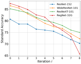
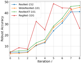
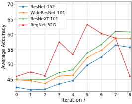
Also, we conducted experiments, as in Figure 4, to select (number of iterations for iterative smoothing) of NCIS for each classification model. Considering average of standard and robust accuracy, is the best iteration number for ResNet-152 [9], WideResNet-101 [18] and ResNeXT-101 [17] and is best for RegNet-32G [14]. Note that, for all experiments, the selected for each classification model was used fixedly.
2.4 Finding the best configuration of NCIS
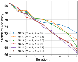
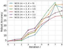
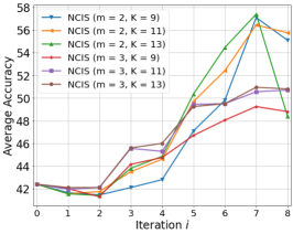
Figure 5 shows the experimental results of various types of NCIS. Note that all NCIS are trained with 5% images of ImageNet training dataset as already proposed in the previous section. First, both robust and standard accuracy of NCIS with is clearly lower than NCIS with because reconstruction difficulty increases as the reshape size of FBI-E becomes bigger. Second, among the results of NCIS with at , NCIS (, ) achieves slightly better performance compared to NCIS (, ). However, robust accuracy of both NCIS (, ) and NCIS (, ) significantly decrease at where NCIS (, ) does not. In this regard, we are concerned that NCIS (, ) and NCIS (, ) might be sensitive to the number of iterations even though they are slightly ahead in performance. Therefore, we selected NCIS (, ) as the representative model of NCIS and conducted all experiments with it.
3 Additional Experimental Results
3.1 Comparison of inference time, GPU memory, and the number of parameters
Table 2 shows the comparison of inference time, GPU memory requirement, and the number of parameters for purifying a single image. GPU memory was measured on an image of size 224x224. First, we can check that traditional input transformation-based methods consistently show fast inference time, except for TVM [15], with no GPU memory requirement. However, as already proposed in the manuscript and [8], these methods are easily broken by strong white-box attacks. Second, the original NRP has a large number of parameters and requires a huge GPU memory for purifying a single image. We think this is a fatal weakness from a practical point of view. To overcome this limitation, the author of NRP newly proposed a lightweight version of NRP, denoted as NRP (resG), at their official code. NRP (resG) significantly reduces inference time, GPU memory requirement, and the number of parameters. However, both NRP and NRP (resG) have the generalization issue and cannot purify several types of adversarial examples well, as proposed in the manuscript. In addition, NCIS is slower than NRP (resG), but shows faster inference time and memory requirements than NRP. Note that the number of parameters of NCIS is significantly lower than NRP variants. GS is the most computationally efficient compared to other baselines. Even though our NCIS is slow and has high computational cost than GS and NRP (resG), we would like to emphasize that NCIS generally achieved superior results against various attacks than GS, and also much better results than both NRP and NRP (resG) when considering both standard and robust accuracy, as already shown in the manuscript.
| JPEG | FS | TVM | SR |
|
NRP |
|
|
|||||||
|---|---|---|---|---|---|---|---|---|---|---|---|---|---|---|
|
0.0070 | 0.0007 | 1.1259 | 0.0084 | 0.0007 | 0.0892 | 0.0004 | 0.0779 | ||||||
|
- | - | - | - | 0.43G | 9.86G | 0.002G | 0.60G | ||||||
| # of Parameters | - | - | - | - | 1.70M | 16.6M | - | 0.40M |
3.2 White-box PGD attack on other classification models
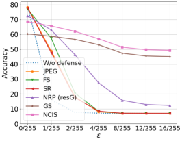
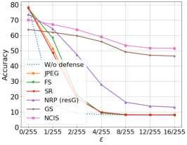
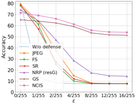
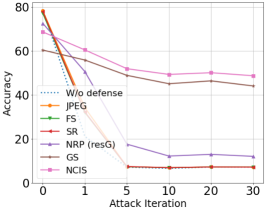
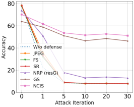
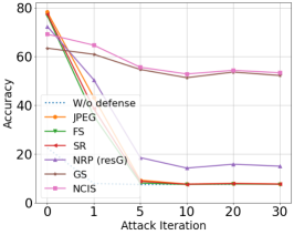
Figure 6 shows additional experimental results against white-box attacks on other classification models. We clearly observe that our proposed methods surpass other baselines on all classification models. Notably, we see that the performance gap between NCIS and GS is slightly wider than the gap on ResNet-152 which was shown in the manuscript. We believe these results show our methods generally purify overall adversarial examples generated from various types of the classification model.
3.3 Transfer-based black-box attack on other classification models
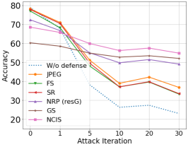
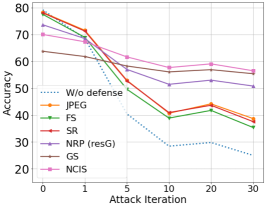
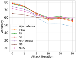
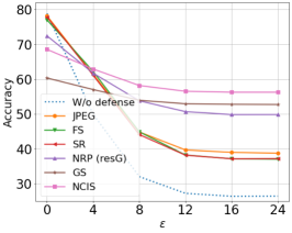
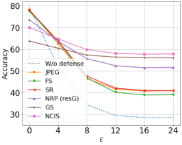
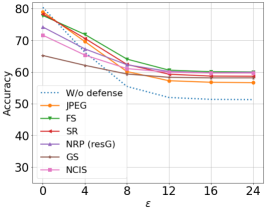
Following the manuscript, Figure 7 shows the experimental results against transfer-based black-box attacks on other classification models. We set a substitute model for each classification model and generated adversarial examples by attacking it. The experimental results demonstrate that GS and NCIS achieve superior results than NRP (resG) in most cases. Also, the same result is shown once again that the performance gap between NCIS and GS is slightly wider than the gap on WideResNet-101. Note that transfer-based black-box attacks on RegNet-32G were not as successful as attacks on other classification models so that there is not much difference in robust accuracy between defense methods.
3.4 Score-based black-box attack
| Model / Defense | Square () | Square () | |||
|---|---|---|---|---|---|
| ResNet-152 |
|
38.00 | 37.68 | ||
| JPEG | 58.81 | 63.20 | |||
| FS | 62.57 | 63.68 | |||
| TVM | 51.23 | 58.05 | |||
| SR | 58.99 | 60.04 | |||
| NRP (resG) | 53.10 | 59.25 | |||
| GS | 55.31 | 51.57 | |||
| NCIS | 58.52 | 55.95 | |||
Following the suggestion of [4], we evaluate both baselines and our proposed method against score-based black-box attack. We select Square [1], which is the state-of-the-art and query efficient black-box attack method, for the experiment. For Square attack, we set with 300 queries and, for Square attack, we set with 300 queries. Other hyperparameters are set to default values as [10].
Figure 3 shows the experimental results against and Square attacks. First, we observe that attack success rate of Square is still low compared to transfer-based black-box attacks and it requires more than 300 queries to successfully fool the classification model. Second, as already shown in [7], the traditional input transformation-based methods (e.g. JPEG, FS, TVM and SR) show robust performance compared to others, such as white-box and transfer-based black-box attacks. Third, our proposed methods (NCIS and GS) and NRP (resG) accomplish competitive performance, and NCIS consistently surpasses GS. When comparing NCIS with NRP (resG), we observe that NCIS obtain higher robust accuracy than NRP (resG) in Square () but lower robust accuracy in Square ().
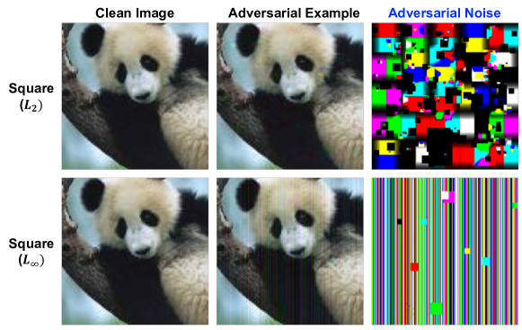
As an analysis, we visualized adversarial examples and noises generated by Square attack in Figure 8. We numerically checked that the mean of the adversarial noise of an entire image is almost zero. However, the figure clearly shows that adversarial noise generated by Square has a structured noise different from adversarial noise generated by the optimization-based white-box attack (e.g PGD). We believe that this is the reason why both our proposed method and NRP (resG) show lower performance compared to input transformation-based methods, this type of adversarial noise is not a form considered in both methods.
3.5 Experimental results with dynamic inference against the purifier-aware white-box attack
| ResNet-152 | Standard Accuracy | White-box PGD | BPDA [2] White-box PGD |
|---|---|---|---|
| NRP (resG) | 66.56 | 37.30 | 33.52 |
| GS | 63.06 | 44.46 | 7.90 |
| NCIS () | 66.58 | 45.64 | 24.56 |
| NCIS () | 61.20 | 48.42 | 33.20 |
Even though our paper focuses on the purifier-blind white-box attack, we conducted experiments on the purifier-aware white-box attack (in other words, strong adaptive attack [2, 16]) by following the suggestion of [16]. We used BPDA [2] implemented in [6] for the purifier-aware white-box attack and applied it to PGD attack. We used randomly sampled 10% data of ImageNet validation dataset and used untargeted PGD attack () with 10 attack iterations for all experiments. We applied dynamic inference against BPDA white-box attack as proposed in the Supplementary Material of NRP [13] to our methods and implemented it by referring their code. Same as default hyperparameters, we set for dynamic inference to and add Gaussian noise with zero mean and to a given input image at each inference.
Table 4 shows the experimental results. We experimentally found that when dynamic inference is applied, the optimal number of iterations ( or ) for NCIS changes from the original number ( for ResNet-152) because of the added noises to the given input image. From the table, we observe that NRP (resG) and NCIS () achieves superior standard accuracy. Besides, we clearly observe once again that for the purifier-blind white-box PGD attack (the results of White-box PGD in the table), NCIS and GS outperform NRP (resG). Moreover, in BPDA white-box PGD attack, GS shows a significant drop in performance but NCIS () shows a competitive robust accuracy compared to NRP (resG).
In conclusion, though we mainly consider the purifier-blind white-box attack, our NCIS can be robust to not only the purifier-blind attack but also the purifier-aware attack using BPDA, by easily applying dynamic inference proposed in the NRP paper.
4 Additional Details on API Experiments
4.1 Dataset generation
For generating benchmark datasets, we sampled images from ImageNet training dataset and generated adversarial examples of it using transfer-based black-box attack using ensemble of five classification models, ResNet-152, VGG-19, GoogleNet, ResNeXT-101, WideResNet-101, based on [11]. We attacked each image with targeted PGD attack with 10 attack iterations, and then made a pair of a clean and an adversarial example. Then, we queried each pair and stored them only when all the top five predicted labels of the clean and adversarial example were totally different. The above process was performed on all the four APIs, and we respectively sampled 100 pairs for test dataset and 20 pairs for validation dataset. In other words, we sampled 100 pairs of test dataset and 20 pairs of validation dataset for each API respectively. We will open all generated datasets publicly.
4.2 Evaluation metrics
First, Prediction Accuracy is the measure for the same number of labels among top five labels between the predicted label of the purified image and the predicted label of the clean image. Second, Top-1 Accuracy is the measure for whether the Top-1 label of the purified image is same as the Top-1 label of the clean image. Finally, Top-5 Accuracy is the measure for whether the Top-1 label of the clean image exists within the Top-5 predicted labels of the purified image.
4.3 Hyperparameter selection
|
AWS | Azure | Clarifai | |||
|---|---|---|---|---|---|---|
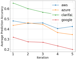
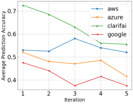
| GS | 0.48 () | 0.46 () | 0.65 () | 0.32 () | ||
| NCIS | 0.58 () | 0.51 () | 0.73 () | 0.48 () |
For GS and NCIS, we found the number of iterations for each API by using the generated validation dataset. As a criterion, we only consider highest average Prediction Accuracy of a clean and adversarial example to select best . Figure 9 shows the experimental results and Table 5 selected best for each dataset. Note that all selected are used for the experiments for APIs in the manuscript.
4.4 Additional qualitative results
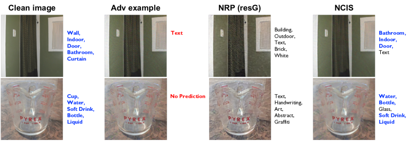
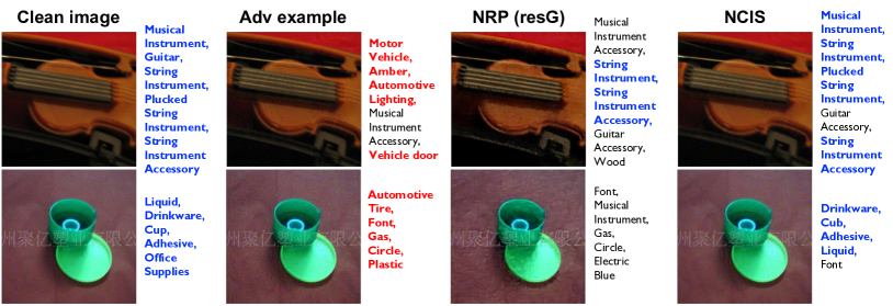
5 Limitations of our work
Even though we proposed a novel and efficient method for adversarial purification, we think that our work also has some limitations as follows. First, our NCIS is effective for purifying adversarial examples generated by optimization-based attacks, which has an almost zero mean and symmetric distribution in a patch, but shows the limitation to purify adversarial examples generated by score-based black-box attacks, which have structured adversarial noises. Second, despite many improvements in inference time and computational cost, NCIS is still slow and requires expensive cost compared to traditional input transformation-based methods. We believe that future studies to overcome these limitations will provide a new direction for achieving adversarial robustness of classification models in a more practical way.
References
- [1] Maksym Andriushchenko, Francesco Croce, Nicolas Flammarion, and Matthias Hein. Square attack: a query-efficient black-box adversarial attack via random search. In European Conference on Computer Vision, pages 484–501. Springer, 2020.
- [2] Anish Athalye, Nicholas Carlini, and David Wagner. Obfuscated gradients give a false sense of security: Circumventing defenses to adversarial examples. In International conference on machine learning, pages 274–283. PMLR, 2018.
- [3] Jaeseok Byun, Sungmin Cha, and Taesup Moon. Fbi-denoiser: Fast blind image denoiser for poisson-gaussian noise. arXiv preprint arXiv:2105.10967, 2021.
- [4] Nicholas Carlini, Anish Athalye, Nicolas Papernot, Wieland Brendel, Jonas Rauber, Dimitris Tsipras, Ian Goodfellow, Aleksander Madry, and Alexey Kurakin. On evaluating adversarial robustness. arXiv preprint arXiv:1902.06705, 2019.
- [5] Nicholas Carlini and David Wagner. Towards evaluating the robustness of neural networks. In 2017 ieee symposium on security and privacy (sp), pages 39–57. IEEE, 2017.
- [6] Gavin Weiguang Ding, Luyu Wang, and Xiaomeng Jin. AdverTorch v0.1: An adversarial robustness toolbox based on pytorch. arXiv preprint arXiv:1902.07623, 2019.
- [7] Yinpeng Dong, Qi-An Fu, Xiao Yang, Tianyu Pang, Hang Su, Zihao Xiao, and Jun Zhu. Benchmarking adversarial robustness on image classification. In Proceedings of the IEEE/CVF Conference on Computer Vision and Pattern Recognition, pages 321–331, 2020.
- [8] Chuan Guo, Mayank Rana, Moustapha Cisse, and Laurens Van Der Maaten. Countering adversarial images using input transformations. arXiv preprint arXiv:1711.00117, 2017.
- [9] Kaiming He, Xiangyu Zhang, Shaoqing Ren, and Jian Sun. Deep residual learning for image recognition. In Proceedings of the IEEE conference on computer vision and pattern recognition, pages 770–778, 2016.
- [10] Hoki Kim. Torchattacks: A pytorch repository for adversarial attacks. arXiv preprint arXiv:2010.01950, 2020.
- [11] Yanpei Liu, Xinyun Chen, Chang Liu, and Dawn Song. Delving into transferable adversarial examples and black-box attacks. arXiv preprint arXiv:1611.02770, 2016.
- [12] Aleksander Madry, Aleksandar Makelov, Ludwig Schmidt, Dimitris Tsipras, and Adrian Vladu. Towards deep learning models resistant to adversarial attacks. arXiv preprint arXiv:1706.06083, 2017.
- [13] Muzammal Naseer, Salman Khan, Munawar Hayat, Fahad Shahbaz Khan, and Fatih Porikli. A self-supervised approach for adversarial robustness. In Proceedings of the IEEE/CVF Conference on Computer Vision and Pattern Recognition, pages 262–271, 2020.
- [14] Ilija Radosavovic, Raj Prateek Kosaraju, Ross Girshick, Kaiming He, and Piotr Dollár. Designing network design spaces. In Proceedings of the IEEE/CVF Conference on Computer Vision and Pattern Recognition, pages 10428–10436, 2020.
- [15] Leonid I Rudin, Stanley Osher, and Emad Fatemi. Nonlinear total variation based noise removal algorithms. Physica D: nonlinear phenomena, 60(1-4):259–268, 1992.
- [16] Florian Tramer, Nicholas Carlini, Wieland Brendel, and Aleksander Madry. On adaptive attacks to adversarial example defenses. arXiv preprint arXiv:2002.08347, 2020.
- [17] Saining Xie, Ross Girshick, Piotr Dollár, Zhuowen Tu, and Kaiming He. Aggregated residual transformations for deep neural networks. In Proceedings of the IEEE conference on computer vision and pattern recognition, pages 1492–1500, 2017.
- [18] Sergey Zagoruyko and Nikos Komodakis. Wide residual networks. arXiv preprint arXiv:1605.07146, 2016.