The statistical geometry of material loops in turbulence

Lukas Bentkamp Max Planck Institute for Dynamics and Self-Organization, Am Faßberg 17, 37077 Göttingen, Germany Theoretical Physics I, University of Bayreuth, Universitätsstraße 30, 95447 Bayreuth, Germany    Theodore D. Drivas Mathematics Department, Stony Brook University, 100 Nicolls Rd., Stony Brook, NY 11794, USA School of Mathematics, Institute for Advanced Study, 1 Einstein Dr., Princeton, NJ 08540, USA    Cristian C. Lalescu Max Planck Institute for Dynamics and Self-Organization, Am Faßberg 17, 37077 Göttingen, Germany Max Planck Computing and Data Facility, Gießenbachstraße 2, 85748 Garching b. München, Germany    Michael Wilczek michael.wilczek@uni-bayreuth.de Max Planck Institute for Dynamics and Self-Organization, Am Faßberg 17, 37077 Göttingen, Germany Theoretical Physics I, University of Bayreuth, Universitätsstraße 30, 95447 Bayreuth, Germany
Abstract

Abstract Material elements – which are lines, surfaces, or volumes behaving as passive, non-diffusive markers – provide an inherently geometric window into the intricate dynamics of chaotic flows. Their stretching and folding dynamics has immediate implications for mixing in the oceans or the atmosphere, as well as the emergence of self-sustained dynamos in astrophysical settings. Here, we uncover robust statistical properties of an ensemble of material loops in a turbulent environment. Our approach combines high-resolution direct numerical simulations of Navier-Stokes turbulence, stochastic models, and dynamical systems techniques to reveal predictable, universal features of these complex objects. We show that the loop curvature statistics become stationary through a dynamical formation process of high-curvature folds, leading to distributions with power-law tails whose exponents are determined by the large-deviations statistics of finite-time Lyapunov exponents of the flow. This prediction applies to advected material lines in a broad range of chaotic flows. To complement this dynamical picture, we confirm our theory in the analytically tractable Kraichnan model with an exact Fokker-Planck approach.

\EdefEscapeHexIntroduction.1Introduction.1\EdefEscapeHexIntroductionIntroduction\hyper@anchorstartIntroduction.1\hyper@anchorendIntroduction

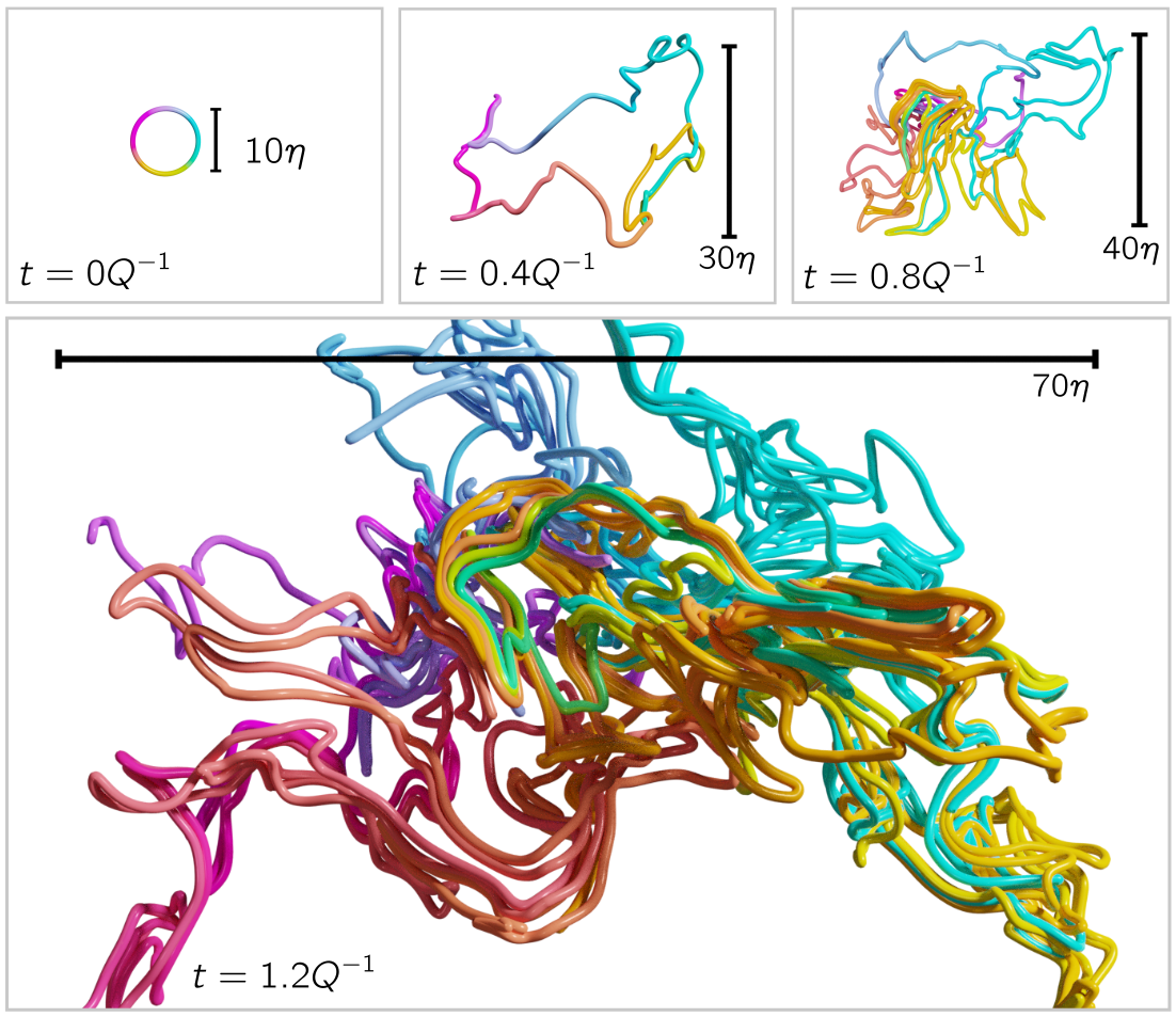
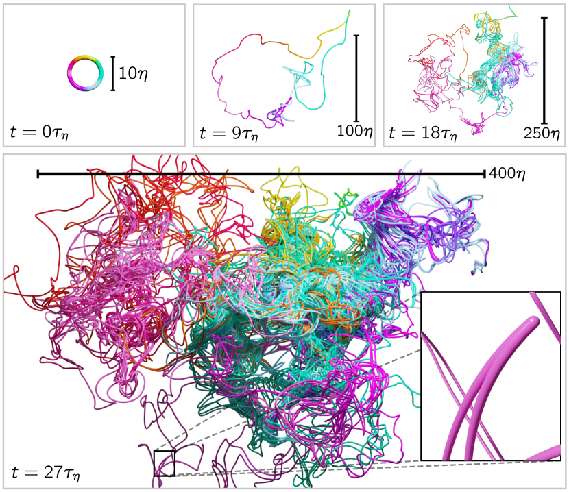
Chaotic flows tend to fold, writhe, and wrinkle material elements into a state of seemingly infinite complexity over time (see Fig. 1 and supplementary movie). A fundamental question is whether this tumultuous process has any predictable features which persist over long periods of time. Answering this question provides insights into the process of mixing which occurs in a whole range of systems, from the diffusion of dye into water, the dispersion of plankton colonies on the ocean surface, to the blast propagation in supernovae thermonuclear explosions [1]. Material lines and interfaces, in particular, provide idealized descriptions of nutrient, temperature and salinity fronts in the oceans [2], and potential vorticity fronts in the atmosphere [3]. They are also closely related to the dynamics of vorticity filaments in fully developed turbulence [4, 5], the conformation of polymer chains [6, 7, 8], the dynamics of flexible phytoplankton chains [9], as well as the motion of magnetic field lines at high conductivity (or high magnetic Reynolds numbers) [10]. The latter is related to the dynamo problem, in which chaotic stretching, folding, and twisting processes are essential for sustaining the growth of a magnetic field. The progress we make in understanding how material elements react to turbulent flows stands to advance our understanding of these fundamental problems.
Refer to caption
Figure 1: Visualization of material loop evolution. The initially circular loop (color corresponds to initial angle) is advected by a turbulent flow field for 27τη27subscript𝜏𝜂27\tau_{\eta}, where τηsubscript𝜏𝜂\tau_{\eta} is the Kolmogorov time. The twisting and folding action of the turbulent flow creates a complex loop geometry while the length of the loop increases exponentially on average (cf. Fig. 3). The loop shown is a comparably extreme case; loops in less turbulent regions develop an extended and complex structure after a longer time. Inset: material fold causing a peak of curvature. (See also supplementary movie)

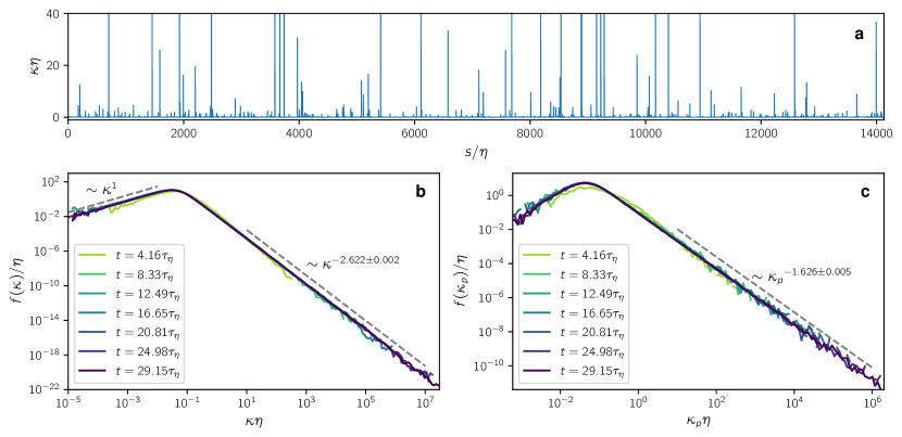
The geometry of material objects advected and deformed by a turbulent flow can be very complex. While volumes are preserved by incompressible flows, the length of lines and the area of surfaces typically grow exponentially [11, 12, 13, 14, 15], with their geometry appearing fractal [16, 17, 18]. Since any curve in space is uniquely described by its curvature and torsion [19], there have been numerous works attempting to characterize the curvature of material lines but also of material surfaces [20, 21, 22, 23, 24, 25, 26, 27, 28, 29, 30, 31, 32, 33, 34] and Lagrangian trajectories [35, 36, 37]. Although material lines seem to become unfathomably complicated over time, the above works suggest that curvature distributions do in fact settle down to a well defined stationary state which features robust power-law tails (see Fig. 2), sparking hope that certain features can be predicted by theory.
Refer to caption
Figure 2: Localized peaks of curvature along the loop cause heavy-tailed curvature distributions. a Curvature along a material loop at t=29.15τη𝑡29.15subscript𝜏𝜂t=29.15\tau_{\eta} as a function of arc length s𝑠s. The function is highly spiked, indicating that high curvature only occurs in isolated narrow regions. These isolated peaks contribute to the high-curvature tails of the curvature PDF. b Curvature PDF of material loops at times t=4.16τη𝑡4.16subscript𝜏𝜂t=4.16\tau_{\eta} (light green) up to t=29.15τη𝑡29.15subscript𝜏𝜂t=29.15\tau_{\eta} (violet). c PDF of curvature peaks of material loops at the same times. The high-curvature regime is fitted by power laws in the regions indicated by the dashed lines by means of a linear fit to the logarithm of the PDF using binomial error estimates.

Here we present a line of arguments based on the dynamical mechanism of sling or fold (i.e. curvature peak) formation and its relation to finite-time Lyapunov exponents that leads to a quantitative prediction of the power law of the curvature distribution observed in Fig. 2, panels b and c. We show that the high-curvature regime of the material line can be understood as an ensemble of persistent parabolic folds, which are formed by random stretching of the line. In this way, we illustrate how understanding dynamical mechanisms can be used to make deductions about statistical geometry. For example, our predicted curvature PDF power-law exponent 2.54±0.11plus-or-minus2.540.11-2.54\pm 0.11 (3%percent33\% relative error to the measured exponent) implies that, in the long-time limit, the average curvature along advected loops is finite but all higher moments diverge. The only input of our theory is the distribution of Lyapunov exponents of the underlying flow field and, as such, our results apply to a wide range of chaotic dynamics. Our predictions are confirmed by direct numerical simulations of fully developed homogeneous, isotropic Navier-Stokes turbulence as well as by exact results in the analytically solvable Kraichnan model.

\EdefEscapeHexResults.1Results.1\EdefEscapeHexResultsResults\hyper@anchorstartResults.1\hyper@anchorendResults

To investigate the evolution of material loops 𝐋(ϕ,t)𝐋italic-ϕ𝑡\mathbf{L}(\phi,t) in fully developed turbulence, we consider initially circular loops and parameterize them by the initial angle ϕ[0,2π)italic-ϕ02𝜋\phi\in[0,2\pi). Each point of the loop follows the velocity field 𝐮(𝐱,t)𝐮𝐱𝑡\mathbf{u}(\mathbf{x},t) according to the tracer equation

t𝐋(ϕ,t)=𝐮(𝐋(ϕ,t),t).subscript𝑡𝐋italic-ϕ𝑡𝐮𝐋italic-ϕ𝑡𝑡\partial_{t}\mathbf{L}(\phi,t)=\mathbf{u}(\mathbf{L}(\phi,t),t). (1)

The evolution of such a loop is shown in Fig. 1, which illustrates that the loop rapidly grows in length and diameter, while attaining a complex geometry due to the stretching and folding by the underlying turbulent flow.

As a key metric to characterize the geometry of the loop, we here focus on the curvature

κ~(ϕ,t)=|(ϕ2𝐋)×(ϕ𝐋)||ϕ𝐋|3.~𝜅italic-ϕ𝑡superscriptsubscriptitalic-ϕ2𝐋subscriptitalic-ϕ𝐋superscriptsubscriptitalic-ϕ𝐋3\tilde{\kappa}(\phi,t)=\frac{\left|(\partial_{\phi}^{2}\mathbf{L})\times(\partial_{\phi}\mathbf{L})\right|}{\left|\partial_{\phi}\mathbf{L}\right|^{3}}. (2)

Material lines grow non-uniformly in length over time. Hence for an evolving ensemble of loops, the distribution of curvature can be defined in different ways, depending on the probability measure we associate with the points along the loop. A simple way of defining the probability density function (PDF) of curvature f(κ;t)𝑓𝜅𝑡f(\kappa;t), that does not depend on the initial parameterization, is to take curvature samples uniformly along the arc length of the loops. Specifically,

f(κ;t)=1L(t)0L(t)dsδ(κκ~(s,t))𝑓𝜅𝑡1delimited-⟨⟩𝐿𝑡delimited-⟨⟩superscriptsubscript0𝐿𝑡d𝑠𝛿𝜅~𝜅𝑠𝑡f(\kappa;t)=\frac{1}{\langle L(t)\rangle}\left\langle\int_{0}^{L(t)}\operatorname{d\!}s\ \delta(\kappa-\tilde{\kappa}(s,t))\right\rangle (3)

where δ𝛿\delta is the Dirac delta function, L(t)𝐿𝑡L(t) is the length of the loop at time t𝑡t and κ~(s,t)~𝜅𝑠𝑡\tilde{\kappa}(s,t) is the curvature of the loop as a function of arc length s𝑠s at time t𝑡t. The average delimited-⟨⟩\langle\cdot\rangle is taken to be uniform over loops, and we have here used κ~~𝜅\tilde{\kappa} to distinguish the loop (realization) dependent curvature from its sample-space variable κ𝜅\kappa.

We use fully resolved turbulence simulations to investigate this measure of the statistical geometry of material lines (see Methods). Here, we focus on a data set at the Taylor-scale Reynolds number Rλ216subscript𝑅𝜆216R_{\lambda}\approx 216, in which we track 1000 randomly placed loops with an initial diameter of 10η10𝜂10\eta (η𝜂\eta is the Kolmogorov length scale). We test the robustness of our results with additional simulations at various Reynolds numbers in Supplementary Note 1.

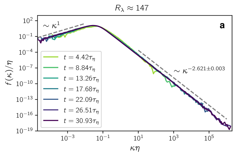
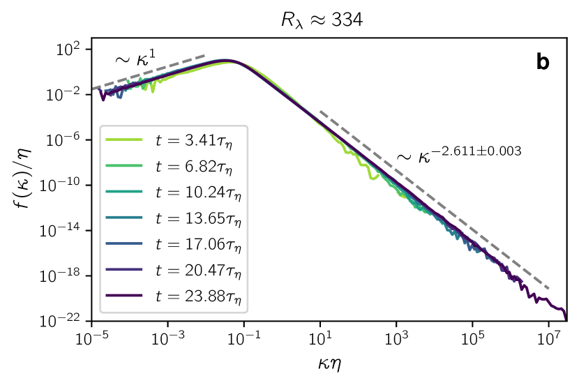
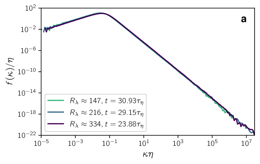
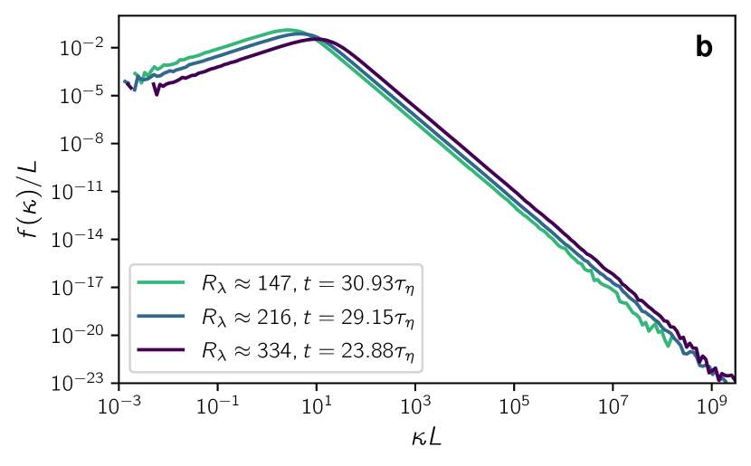
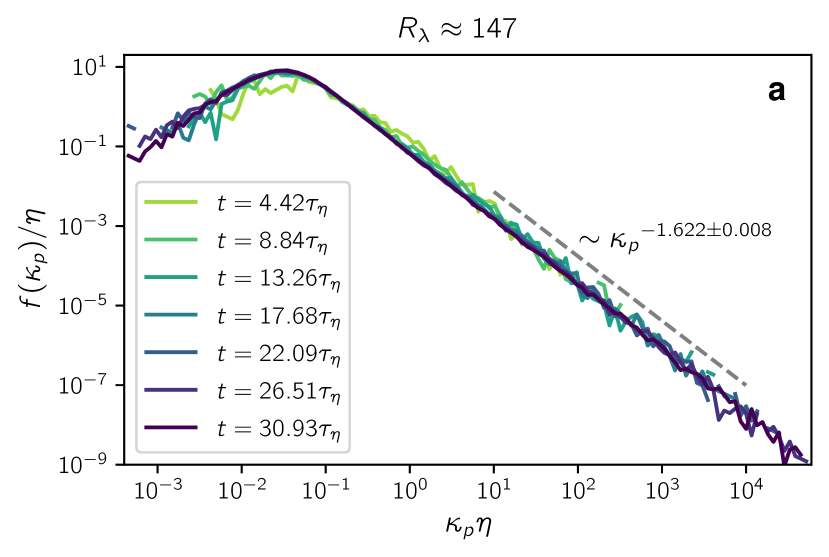
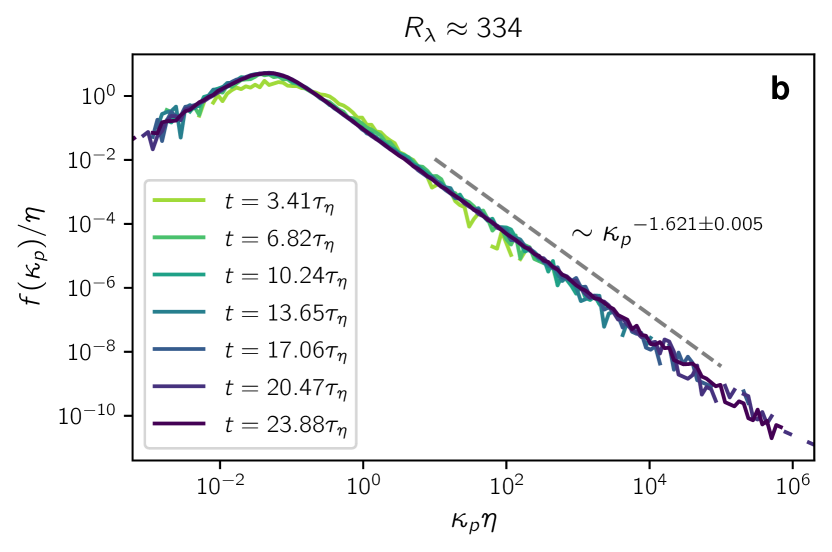
The resulting curvature PDF at different times is shown in Fig. 2b. Remarkably, persistent power-law tails form within a few Kolmogorov time scales τηsubscript𝜏𝜂\tau_{\eta}, which eventually range over several decades of curvature after the loops have been deformed for 29τη29subscript𝜏𝜂29\tau_{\eta} (1.5similar-toabsent1.5\sim 1.5 integral times). Within this observation window, the shape of the distribution appears to become stationary, whereas the support, i.e. the range from minimum to maximum curvature, grows indefinitely in extent. Hence the largest curvatures correspond to structures significantly smaller than the Kolmogorov length scale η𝜂\eta. As we show in Supplementary Note 1, the distributions are almost indistinguishable for different Reynolds numbers when nondimensionalized by η𝜂\eta, but they shift to larger κ𝜅\kappa when displayed in units of the integral length. This is a first indication that the curvature distribution is generated by the smallest scales of the flow, in particular by velocity gradients. Given the markedly complex shape of the deformed material loop, the universal shape of the distribution calls for a theoretical explanation, which we develop in the following.

Ensemble of material folds

The high-curvature regime of the curvature distribution is heavy-tailed and characterized by rare events. Over time, the material line will form isolated sites of extremely high curvature [30, 31, 33, 32, 34], as can be seen in Fig. 2a. Such curvature peaks mark sharp folds in the material line geometry. In the following, we reveal how such folds form stochastically and how this is related to the power-law exponent of the curvature distribution.

This picture in view, we estimate the high-curvature tail of the PDF (3) in the statistically steady state by replacing the ensemble average over entire loops in (3) by an ensemble of folds,

f(κ)0dκpf(κp)dsδ(κκpb(s;κp)).similar-to𝑓𝜅superscriptsubscript0dsubscript𝜅𝑝𝑓subscript𝜅𝑝superscriptsubscriptd𝑠𝛿𝜅superscript𝜅pb𝑠subscript𝜅𝑝\displaystyle f(\kappa)\sim\int_{0}^{\infty}\operatorname{d\!}\kappa_{p}~{}f(\kappa_{p})\int_{-\infty}^{\infty}\operatorname{d\!}s~{}\delta\left(\kappa-\kappa^{\text{pb}}(s;\kappa_{p})\right). (4)

Here, κpsubscript𝜅𝑝\kappa_{p} is the peak curvature of a fold and f(κp)𝑓subscript𝜅𝑝f(\kappa_{p}) its distribution. The second integral is the contribution of curvature around each curvature peak. As we will elaborate in more detail below, high-curvature folds develop a universal, locally parabolic shape. The curvature function around a peak with maximum κpsubscript𝜅𝑝\kappa_{p}, therefore, can be estimated as [32]

κpb(s;κp)superscript𝜅pb𝑠subscript𝜅𝑝\displaystyle\kappa^{\text{pb}}(s;\kappa_{p}) =κp(1+F1(|κps|)2)3/2,absentsubscript𝜅𝑝superscript1superscript𝐹1superscriptsubscript𝜅𝑝𝑠232\displaystyle=\frac{\kappa_{p}}{\left(1+F^{-1}(|\kappa_{p}s|)^{2}\right)^{3/2}}, (5)

where F1(x)superscript𝐹1𝑥F^{-1}(x) denotes the inverse of the primitive of 1+x21superscript𝑥2\sqrt{1+x^{2}} on the positive real line, originating from parameterizing the parabola by arc length. Remarkably, the curvature profile is characterized by the peak curvature as the only parameter. To further evaluate (4), we substitute the inner integration variable by κ=κpb(s;κp)superscript𝜅superscript𝜅pb𝑠subscript𝜅𝑝\kappa^{\prime}=\kappa^{\text{pb}}(s;\kappa_{p}) with the Jacobian

|dspb(κ;κp)dκ|=13κ2(κp/κ)2/31,dsuperscript𝑠pbsuperscript𝜅subscript𝜅𝑝dsuperscript𝜅13superscript𝜅2superscriptsubscript𝜅𝑝superscript𝜅231\displaystyle\left|\mathinner{\dfrac{\operatorname{d\!}{}s^{\text{pb}}(\kappa^{\prime};\kappa_{p})}{\operatorname{d\!}{\kappa^{\prime}}}}\right|=\frac{1}{3\kappa^{\prime 2}\sqrt{(\kappa_{p}/\kappa^{\prime})^{2/3}-1}}, (6)

which yields

f(κ)𝑓𝜅\displaystyle f(\kappa) κdκpf(κp)|dspb(κ;κp)dκ|.similar-toabsentsuperscriptsubscript𝜅dsubscript𝜅𝑝𝑓subscript𝜅𝑝dsuperscript𝑠pb𝜅subscript𝜅𝑝d𝜅\displaystyle\sim\int_{\kappa}^{\infty}\operatorname{d\!}\kappa_{p}~{}f(\kappa_{p})\left|\mathinner{\dfrac{\operatorname{d\!}{}s^{\text{pb}}(\kappa;\kappa_{p})}{\operatorname{d\!}{\kappa}}}\right|. (7)

This equation expresses the curvature PDF as a composition of the curvature peak PDF with the contribution from the locally parabolic folds.

Statistical evolution of curvature peaks

In what follows, we determine the curvature peak distribution f(κp)𝑓subscript𝜅𝑝f(\kappa_{p}), which can be achieved by capturing the essence of the curvature peak dynamics. Since peaks are generally generated at medium curvature and then grow stochastically, we may define the generation time t0subscript𝑡0t_{0} of a large peak as the time where it has first surpassed an (arbitrary) threshold κ0subscript𝜅0\kappa_{0} and its age as τ=tt0𝜏𝑡subscript𝑡0\tau=t-t_{0}. At time t𝑡t, the ensemble of peaks larger than κ0subscript𝜅0\kappa_{0} can thus be attributed a distribution of ages f(τ;t)𝑓𝜏𝑡f(\tau;t). By the law of total probability, the peak distribution above κ0subscript𝜅0\kappa_{0} can be estimated as

f(κp;t)𝑓subscript𝜅𝑝𝑡\displaystyle f(\kappa_{p};t) 0tdτf(κp|τ)f(τ;t),similar-toabsentsuperscriptsubscript0𝑡d𝜏𝑓conditionalsubscript𝜅𝑝𝜏𝑓𝜏𝑡\displaystyle\sim\int_{0}^{t}\operatorname{d\!}\tau~{}f(\kappa_{p}|\tau)f(\tau;t), (8)

where f(κp|τ)𝑓conditionalsubscript𝜅𝑝𝜏f(\kappa_{p}|\tau) is the probability of a peak with curvature κ0subscript𝜅0\kappa_{0} at time t0subscript𝑡0t_{0} to have curvature κpsubscript𝜅𝑝\kappa_{p} at time t0+τsubscript𝑡0𝜏t_{0}+\tau. This decomposes the curvature peak distribution into a distribution of peaks with a given age and the distribution of ages. In (7), we are interested in the stationary regime f(κp):=limtf(κp;t)f(\kappa_{p})\mathrel{\mathop{\mathchar 58\relax}}=\lim_{t\to\infty}f(\kappa_{p};t), which we expect to be well captured by the estimate (8) and to be independent of the arbitrary threshold κ0subscript𝜅0\kappa_{0}.

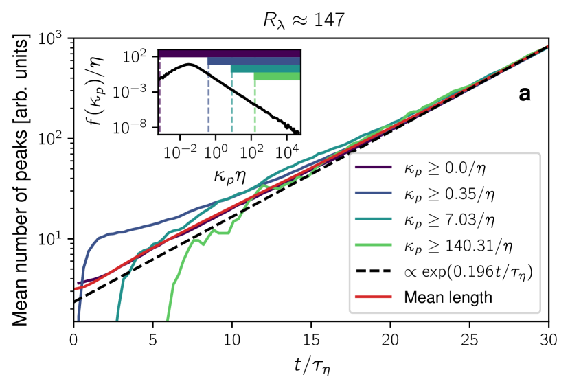
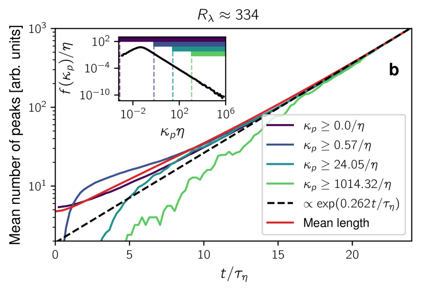
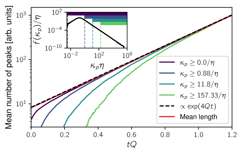
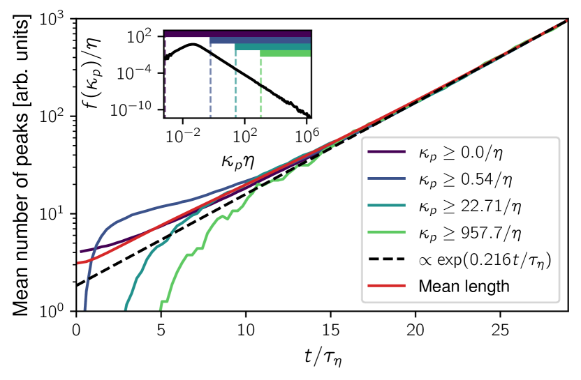
The peak age distribution can be estimated from the mean number of curvature peaks. Figure 3 shows that the mean numbers of curvature maxima above different thresholds grow at the same exponential rate β0.216/τη𝛽0.216subscript𝜏𝜂\beta\approx 0.216/\tau_{\eta}, which coincides with the growth rate of the mean length of the loops.
Refer to caption
Figure 3: Mean number of curvature peaks above different thresholds over time. The lines are vertically shifted for comparison, showing that the peaks are generated at a clearly defined exponential rate. Moreover, the curves appear to be asymptotically proportional to the mean arc length of loops (red). The dashed line indicates an exponential fit to the last third of the total peak number curve (violet), yielding the rate β=(0.21619±0.00014)/τη𝛽plus-or-minus0.216190.00014subscript𝜏𝜂\beta=(0.21619\pm 0.00014)/\tau_{\eta}. The standard error of this rate is so small that we neglect it in the following. Note that without vertically shifting the curves in the plot, they would remain ordered as a function of the threshold condition. Inset: Curvature peak distribution at t=29.15τη𝑡29.15subscript𝜏𝜂t=29.15\tau_{\eta} indicating the different thresholds.

Intuitively, this can be explained by the fact that the generation of folds is a random process along the loop. Since the loop length grows on average exponentially over time, so does the number of folds. Neglecting the disappearance of peaks, we, therefore, estimate the probability of a high-curvature fold at time t𝑡t to be generated before some time tsuperscript𝑡t^{\prime} (with 0tt0superscript𝑡𝑡0\leq t^{\prime}\leq t) by the fraction of peaks that existed at tsuperscript𝑡t^{\prime}, given by eβt/eβtsuperscript𝑒𝛽superscript𝑡superscript𝑒𝛽𝑡e^{\beta t^{\prime}}/e^{\beta t}. This cumulative distribution function of peak birth times implies the probability density function of peak age

f(τ;t)𝑓𝜏𝑡\displaystyle f(\tau;t) βeβτ,0τt.formulae-sequenceabsent𝛽superscript𝑒𝛽𝜏0𝜏𝑡\displaystyle\approx\beta e^{-\beta\tau},\qquad 0\leq\tau\leq t. (9)

This shows that, since curvature peaks are generated at an exponential rate, their age distribution also decays exponentially, implying that the bulk of the peaks are young even after a long evolution of the loop.

In the following, we investigate the dynamics and statistics of peak curvature in an effort to estimate the remaining conditional probability f(κp|τ)𝑓conditionalsubscript𝜅𝑝𝜏f(\kappa_{p}|\tau) and form our theory.

Amplification of folds by turbulent stretching

We observe that those rare peaks that have existed for a long time can exhibit extremely high curvature. This is caused by fluid element stretching, a process quantitatively captured by the deformation tensor

Fij(𝐱,t)subscript𝐹𝑖𝑗𝐱𝑡\displaystyle F_{ij}(\mathbf{x},t) =Xi(𝐱,t)xj,absentsubscript𝑋𝑖𝐱𝑡subscript𝑥𝑗\displaystyle=\mathinner{\dfrac{\partial{}X_{i}(\mathbf{x},t)}{\partial{x_{j}}}}, (10)

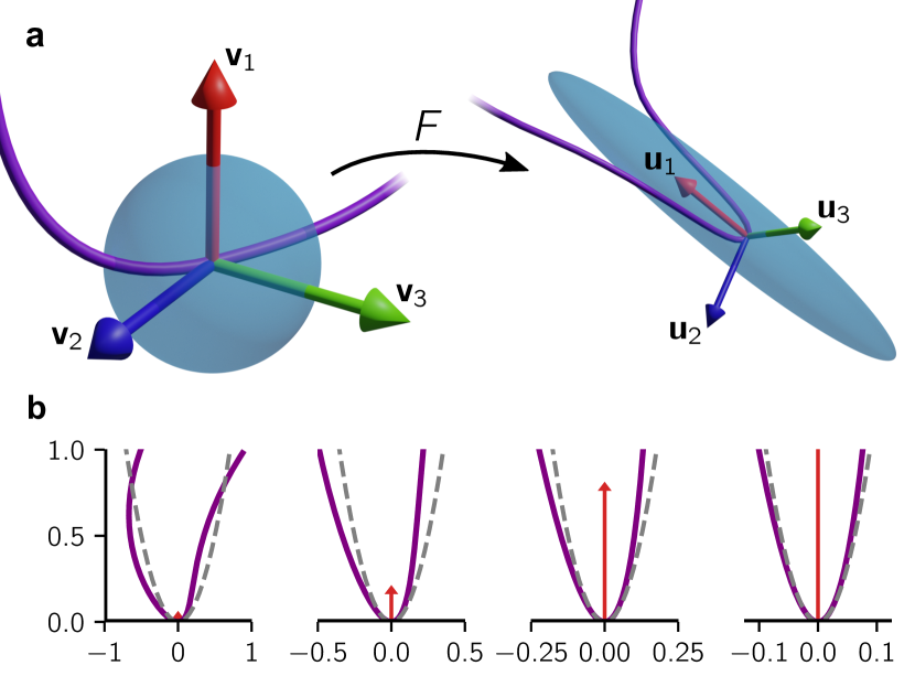
where 𝐗(𝐱,t)𝐗𝐱𝑡\mathbf{X}(\mathbf{x},t) is the Lagrangian map, mapping the initial condition 𝐱𝐱\mathbf{x} of a tracer particle to its position 𝐗𝐗\mathbf{X} at time t𝑡t. The singular value decomposition of the deformation tensor associates two coordinate systems 𝐯isubscript𝐯𝑖\mathbf{v}_{i} and 𝐮isubscript𝐮𝑖\mathbf{u}_{i} with the deformation (see Methods), as illustrated in Fig. 4a. The associated exponential stretching rates are given by the finite-time Lyapunov exponents (FTLE) ρi(t)subscript𝜌𝑖𝑡\rho_{i}(t).

Refer to caption
Figure 4: Formation of a parabolic fold. a Illustration of the deformation tensor F𝐹F. 𝐯isubscript𝐯𝑖\mathbf{v}_{i} denote the principal axes of stretching before deformation and 𝐮isubscript𝐮𝑖\mathbf{u}_{i} the corresponding axes after deformation. A fluid element (blue) will be predominantly stretched along the direction of most stretching 𝐯1subscript𝐯1\mathbf{v}_{1} and compressed in the direction of most compression 𝐯3subscript𝐯3\mathbf{v}_{3} over time. If a material line element (violet) is initially orthogonal to the direction of most stretching, a fold will form. Such a fold is then compressed onto the 𝐮1subscript𝐮1\mathbf{u}_{1}-𝐮2subscript𝐮2\mathbf{u}_{2} plane and tends to align with the 𝐮1subscript𝐮1\mathbf{u}_{1} direction along which it is amplified. b Stretching creates a locally parabolic curve. An initially non-parabolic curve is stretched vertically as indicated by the red arrows. Viewed on the appropriate horizontal scale, the line becomes increasingly parabolic. For comparison, the dashed line indicates a parabola with the same peak curvature.

As discussed in ref. [32], generically a line element will align with the 𝐮1subscript𝐮1\mathbf{u}_{1}-direction and become stretched exponentially with eρ1(t)tsuperscript𝑒subscript𝜌1𝑡𝑡e^{\rho_{1}(t)t} (whose mean asymptotically scales like eβtsuperscript𝑒𝛽𝑡e^{\beta t}). The surrounding curve will be forced into the 𝐮1subscript𝐮1\mathbf{u}_{1}-𝐮2subscript𝐮2\mathbf{u}_{2} plane by compression in the 𝐮3subscript𝐮3\mathbf{u}_{3}-direction. The dominant stretching in the 𝐮1subscript𝐮1\mathbf{u}_{1}-direction locally decreases curvature. However, an exception to this generic setting occurs at a finite number of points along the loop when the initial material line lies perpendicular to 𝐯1subscript𝐯1\mathbf{v}_{1} (see Fig. 4). In this case, the line element cannot align with 𝐮1subscript𝐮1\mathbf{u}_{1} and will align with 𝐮2subscript𝐮2\mathbf{u}_{2} instead. The surrounding curve, however, still experiences the stretching in the 𝐮1subscript𝐮1\mathbf{u}_{1}-direction. This essentially magnifies the local structure of the curve, which will generically result in a parabolic shape, as illustrated in Fig. 4b. Therefore parabolas become increasingly good local approximations of the folds.

To reveal the role of the finite-time Lyapunov exponents, let us consider a parabola y=κ0x2/2𝑦subscript𝜅0superscript𝑥22y=\kappa_{0}x^{2}/2 which is already initially lying in the 𝐯1subscript𝐯1\mathbf{v}_{1}-𝐯2subscript𝐯2\mathbf{v}_{2} plane. Over time, it is subject to stretching y=eρ1(t)tysuperscript𝑦superscript𝑒subscript𝜌1𝑡𝑡𝑦y^{\prime}=e^{\rho_{1}(t)t}y and x=eρ2(t)txsuperscript𝑥superscript𝑒subscript𝜌2𝑡𝑡𝑥x^{\prime}=e^{\rho_{2}(t)t}x, which preserves the parabolic shape, i.e. y=e[ρ1(t)2ρ2(t)]tκ0x2/2superscript𝑦superscript𝑒delimited-[]subscript𝜌1𝑡2subscript𝜌2𝑡𝑡subscript𝜅0superscript𝑥22y^{\prime}=e^{[\rho_{1}(t)-2\rho_{2}(t)]t}\kappa_{0}x^{\prime 2}/2. In this process, the peak curvature increases as long as ρ1(t)>2ρ2(t)subscript𝜌1𝑡2subscript𝜌2𝑡\rho_{1}(t)>2\rho_{2}(t) [32], i.e. the first FTLE must be more than twice as large as the second one. We illustrate this at the example of a parabola in a linearized flow in Methods, showing that its peak curvature grows as

κp(t)t0κ~0e[ρ1(t)2ρ2(t)]tsuperscriptmuch-greater-than𝑡0subscript𝜅𝑝𝑡subscript~𝜅0superscript𝑒delimited-[]subscript𝜌1𝑡2subscript𝜌2𝑡𝑡\displaystyle\kappa_{p}(t)\stackrel{{\scriptstyle t\gg 0}}{{\approx}}\widetilde{\kappa}_{0}e^{[\rho_{1}(t)-2\rho_{2}(t)]t} (11)

for some effective initial peak curvature κ~0subscript~𝜅0\widetilde{\kappa}_{0}. This equation can already be found in ref. [32], where it is derived for a generic material line. Let us call the growth rate of peaks ρp(t)=ρ1(t)2ρ2(t)subscript𝜌𝑝𝑡subscript𝜌1𝑡2subscript𝜌2𝑡\rho_{p}(t)=\rho_{1}(t)-2\rho_{2}(t). In turbulence, this growth rate is typically asymptotically positive. In our simulation used for obtaining the FTLEs (see Methods), we can estimate the infinite-time Lyapunov exponents, λi=limtρi(t)subscript𝜆𝑖subscript𝑡subscript𝜌𝑖𝑡\lambda_{i}=\lim_{t\to\infty}\rho_{i}(t), by taking the mean of the FTLEs at the final time of the simulation, which yields λ10.12/τηsubscript𝜆10.12subscript𝜏𝜂\lambda_{1}\approx 0.12/\tau_{\eta}, λ20.03/τηsubscript𝜆20.03subscript𝜏𝜂\lambda_{2}\approx 0.03/\tau_{\eta}, λ30.15/τηsubscript𝜆30.15subscript𝜏𝜂\lambda_{3}\approx-0.15/\tau_{\eta}, in good agreement with previous literature [38, 39], and thus λp=limtρp(t)0.06/τη>0subscript𝜆𝑝subscript𝑡subscript𝜌𝑝𝑡0.06subscript𝜏𝜂0\lambda_{p}=\lim_{t\to\infty}\rho_{p}(t)\approx 0.06/\tau_{\eta}>0.

Connecting the power-law exponent to fluid stretching

To relate the dynamical formation of folds to the power-law tails of the curvature PDF, we estimate the distribution of κp(t)subscript𝜅𝑝𝑡\kappa_{p}(t) by making statements about the distribution of FTLEs. By ergodicity, FTLEs behave like sums of independent and identically distributed random variables at large times [40, 39]. The same is true for the growth rate of peaks ρp(t)subscript𝜌𝑝𝑡\rho_{p}(t). Using its Cramér function S(ρp)𝑆subscript𝜌𝑝S(\rho_{p}), we make a large-deviations estimate of the PDF,

f(ρp;t)N(t)etS(ρp),𝑓subscript𝜌𝑝𝑡𝑁𝑡superscript𝑒𝑡𝑆subscript𝜌𝑝\displaystyle f(\rho_{p};t)\approx N(t)e^{-tS(\rho_{p})}, (12)

where N(t)𝑁𝑡N(t) is a normalization. Transforming by (11), the peak curvature PDF for peaks of age τ𝜏\tau can thus be written as

f(κp|τ)𝑓conditionalsubscript𝜅𝑝𝜏\displaystyle f(\kappa_{p}|\tau) N(τ)κpτeτS(log(κpκ0)/τ).absent𝑁𝜏subscript𝜅𝑝𝜏superscript𝑒𝜏𝑆subscript𝜅𝑝subscript𝜅0𝜏\displaystyle\approx\frac{N(\tau)}{\kappa_{p}\tau}e^{-\tau S\left(\log\left(\frac{\kappa_{p}}{\kappa_{0}}\right)/\tau\right)}. (13)

Note that we here identified the peak age τ𝜏\tau with the time t𝑡t and the curvature threshold κ0subscript𝜅0\kappa_{0} with the effective initial peak curvature κ~0subscript~𝜅0\widetilde{\kappa}_{0}. For the asymptotics that we are interested in, the distinction does not matter. Inserting this result into (8), combined with (9) and letting t𝑡t\to\infty, gives the asymptotic distribution of curvature peaks in the high-curvature regime

f(κp)0dτeβτN(τ)κpτeτS(log(κpκ0)/τ).similar-to𝑓subscript𝜅𝑝superscriptsubscript0d𝜏superscript𝑒𝛽𝜏𝑁𝜏subscript𝜅𝑝𝜏superscript𝑒𝜏𝑆subscript𝜅𝑝subscript𝜅0𝜏\displaystyle f(\kappa_{p})\sim\int_{0}^{\infty}\operatorname{d\!}\tau~{}e^{-\beta\tau}\frac{N(\tau)}{\kappa_{p}\tau}e^{-\tau S\left(\log\left(\frac{\kappa_{p}}{\kappa_{0}}\right)/\tau\right)}. (14)
Refer to caption
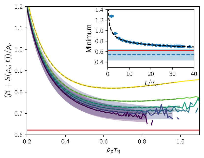
Figure 5: Determination of the steepest-descent minimum. The Cramér function is estimated from FTLE histograms by (12). We call these finite-time estimates S(ρp;t)𝑆subscript𝜌𝑝𝑡S(\rho_{p};t). Here we show the function minimized in (15) for estimates of the Cramér function ranging from t=6.90τη𝑡6.90subscript𝜏𝜂t=6.90\tau_{\eta} (yellow) up to t=39.68τη𝑡39.68subscript𝜏𝜂t=39.68\tau_{\eta} (violet). Best fits are indicated by dashed lines with shaded areas showing their error (see Methods for details). Inset: Minima of these functions over time. A simple fit of the decay of minima (black dashed line) yields an estimate of their limiting value α=0.54±0.11𝛼plus-or-minus0.540.11\alpha=0.54\pm 0.11 (horizontal blue dashed line and shaded area). For comparison, the red lines show the value of α𝛼\alpha estimated by subtracting 2 from the observed curvature PDF power-law exponent in Fig. 2b, showing a good agreement within uncertainties. For more details, see Methods.

We now use the method of steepest descent [41] in order to extract the large-κpsubscript𝜅𝑝\kappa_{p} asymptotics of the peak curvature distribution from our estimate (14). The result (see Methods) is that the distribution scales as a power law, f(κp)κp1αsimilar-to𝑓subscript𝜅𝑝superscriptsubscript𝜅𝑝1𝛼f(\kappa_{p})\sim\kappa_{p}^{-1-\alpha}, with exponent

α=minρp[1ρp(β+S(ρp))].𝛼subscriptsubscript𝜌𝑝1subscript𝜌𝑝𝛽𝑆subscript𝜌𝑝\displaystyle\alpha=\min_{\rho_{p}}\left[\tfrac{1}{\rho_{p}}(\beta+S(\rho_{p}))\right]. (15)

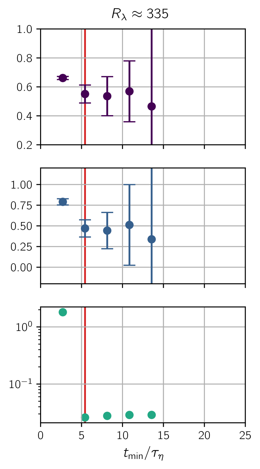
This minimum is estimated for our data in Fig. 5, where the Cramér functions have been estimated via (12) using FTLE histograms from an additional simulation (see Methods). While we are interested in finding the minimum for the fully converged Cramér function, the amount of samples needed to resolve large-deviations statistics increases exponentially with time, limiting our observation window of the minimum to a maximum time of about 30 to 40τη40subscript𝜏𝜂40\tau_{\eta}. In this regime, the minima still lie above the value of α𝛼\alpha inferred from the loops simulation (red line). However, an analysis of the time evolution of minima (Fig. 5, inset) reveals that they are well described by a slow, algebraic decay. Extrapolating the desired minimum towards t𝑡t\to\infty, we get the estimate α=0.54±0.11𝛼plus-or-minus0.540.11\alpha=0.54\pm 0.11, slightly below but within error bars of the curvature peak power-law exponent in Fig. 2c. For more details on the extrapolation, see Methods.

Given the power-law scaling of the peak distribution, f(κp)κp1αsimilar-to𝑓subscript𝜅𝑝superscriptsubscript𝜅𝑝1𝛼f(\kappa_{p})\sim{\kappa_{p}}^{-1-\alpha}, we can perform the integral (7) to obtain the prediction for the curvature PDF

f(κ)κ2α.similar-to𝑓𝜅superscript𝜅2𝛼\displaystyle f(\kappa)\sim\kappa^{-2-\alpha}. (16)

Hence the difference between the curvature power-law exponent and the curvature peak power-law exponent is 1. This difference originates from the curvature contributions of parabolic fold profiles around the peak curvature (5). Comparing Fig. 2b and c shows that this result is consistent with the fully resolved loops simulations. Likewise, our prediction based on Lyapunov exponents estimated by extrapolating the minimum in Fig. 5 captures the observed power-law exponents of both the curvature and curvature peak PDFs very well. In Supplementary Note 1, we explore our result at various Reynolds numbers, with comparable or even better agreement depending on how far the minima can be resolved in time. Therefore, as a central result, we can quantitatively relate the statistical geometry as characterized by the curvature PDF to the formation of folds and the statistics of FTLEs that determine their dynamical evolution.

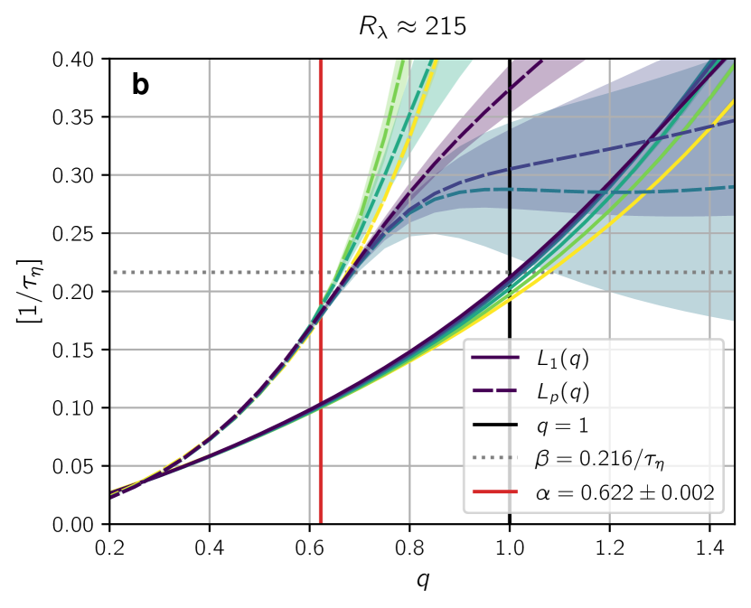
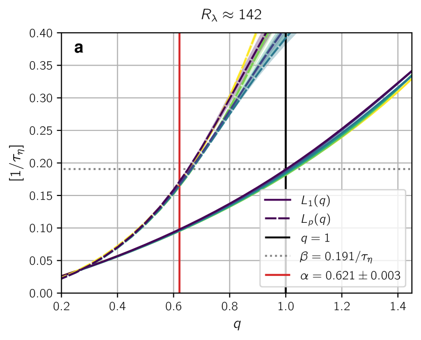
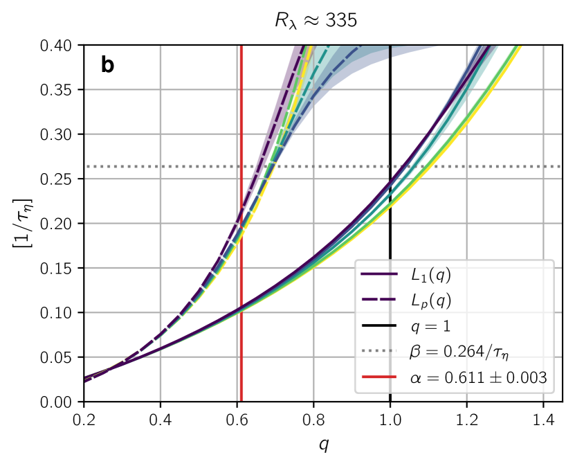
Interestingly, an alternative formulation of our result can be obtained by using the Legendre transform of the Cramér function, which is known as the generalized Lyapunov exponent [39]. It can be shown (see Methods) that α𝛼\alpha is given implicitly by

eαρp(t)tdelimited-⟨⟩superscript𝑒𝛼subscript𝜌𝑝𝑡𝑡\displaystyle\left\langle e^{\alpha\rho_{p}(t)t}\right\rangle eρ1(t)tsimilar-toabsentdelimited-⟨⟩superscript𝑒subscript𝜌1𝑡𝑡\displaystyle\sim\left\langle e^{\rho_{1}(t)t}\right\rangle (17)

in the large-deviations approximation, where similar-to\sim indicates the same exponential scaling for large t𝑡t. This can be understood as the statement that the power-law exponent is chosen so that curvature peak generation (represented by the line growth rate ρ1(t)subscript𝜌1𝑡\rho_{1}(t)) and peak amplification (represented by the peak curvature growth rate ρp(t)=ρ1(t)2ρ2(t)subscript𝜌𝑝𝑡subscript𝜌1𝑡2subscript𝜌2𝑡\rho_{p}(t)=\rho_{1}(t)-2\rho_{2}(t)) are on average balanced. For example, in a flow with the same peak amplification (same statistics of ρp(t)subscript𝜌𝑝𝑡\rho_{p}(t)) but stronger line growth (larger eρ1(t)tdelimited-⟨⟩superscript𝑒subscript𝜌1𝑡𝑡\langle e^{\rho_{1}(t)t}\rangle) and thus stronger peak generation, a larger fraction of small-curvature peaks will accumulate until the stationary state is reached. This means that the curvature PDF in the stationary state has to decay faster, corresponding to a larger α𝛼\alpha, as encoded in (17). We explore this result numerically in Supplementary Note 2, showing that this complementary way of computing α𝛼\alpha comes equally close to the value observed in the loops simulations.

Exact results in the Kraichnan model

To demonstrate the robustness of our results beyond Navier-Stokes turbulence, we consider the exactly solvable Kraichnan model [42]. The Kraichnan model of turbulence replaces the advecting velocity with a spatially correlated Gaussian random field, white in time, which mimics turbulence. While we do not expect the predictions of the curvature PDF power law from the Kraichnan model to be in quantitative agreement with our DNS results, it serves as a test case in which our approach can be compared rigorously against exact independent Fokker-Planck calculations.

In this setting, all of our argumentation about fold formation and its statistical implications can be made exact. First, the Cramér function takes the parabolic form [40]

S(ρp)𝑆subscript𝜌𝑝\displaystyle S(\rho_{p}) =(ρpλp)22Dp,absentsuperscriptsubscript𝜌𝑝subscript𝜆𝑝22subscript𝐷𝑝\displaystyle=\frac{(\rho_{p}-\lambda_{p})^{2}}{2D_{p}}, (18)

with λp=3Qsubscript𝜆𝑝3𝑄\lambda_{p}=3Q, Dp=14Qsubscript𝐷𝑝14𝑄D_{p}=14Q and Q𝑄Q a constant related to the energy spectrum quantifying fluctuations of the velocity gradient (see Methods). λpsubscript𝜆𝑝\lambda_{p} and Dp/tsubscript𝐷𝑝𝑡D_{p}/t are the mean and variance of the Gaussian distribution of ρpsubscript𝜌𝑝\rho_{p} that can be computed from the known multivariate Gaussian distribution of the ρisubscript𝜌𝑖\rho_{i} [40]. Now, the integral (14) can be performed exactly, yielding a power law κp1αsuperscriptsubscript𝜅𝑝1𝛼{\kappa_{p}}^{-1-\alpha} with

α=λpDp+λp2Dp2+2βDp.𝛼subscript𝜆𝑝subscript𝐷𝑝superscriptsubscript𝜆𝑝2superscriptsubscript𝐷𝑝22𝛽subscript𝐷𝑝\displaystyle\alpha=-\frac{\lambda_{p}}{D_{p}}+\sqrt{\frac{\lambda_{p}^{2}}{D_{p}^{2}}+\frac{2\beta}{D_{p}}}. (19)

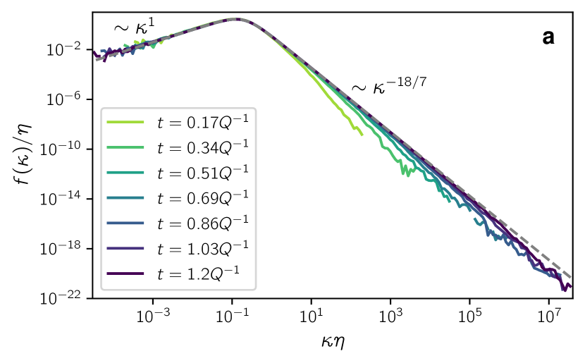
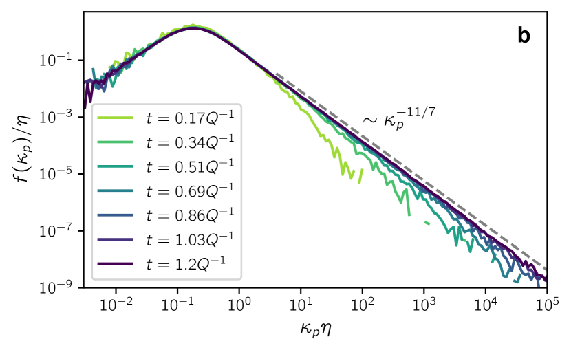
The growth rate of the mean length of line elements in the Kraichnan model is β=4Q𝛽4𝑄\beta=4Q, determined by eβteρ1(t)tsimilar-tosuperscript𝑒𝛽𝑡delimited-⟨⟩superscript𝑒subscript𝜌1𝑡𝑡e^{\beta t}\sim\langle e^{\rho_{1}(t)t}\rangle. This evaluates to α=4/7𝛼47\alpha=4/7, a curvature peak PDF power law 11/7117-11/7 and a curvature PDF power law 18/72.5711872.571-18/7\approx-2.571. Although this is very close to the exponent 2.622±0.002plus-or-minus2.6220.002-2.622\pm 0.002 that we find in Navier-Stokes turbulence, we believe that our measurements are precise enough to conclude that the exponents are in fact different and that their closeness is coincidental.

Importantly, this result based on our picture of curvature growth due to fold formation is consistent with an independent, complementary approach facilitated by the rapidly fluctuating velocity field. Using Itô calculus, one can obtain an exact Fokker-Planck equation for the curvature distribution (see Methods) and study its steady state. The equation takes the form

tf=κ(18Qκf7Qκ2κf+9Pκf9Pκf),subscript𝑡𝑓subscript𝜅18𝑄𝜅𝑓7𝑄superscript𝜅2subscript𝜅𝑓9𝑃𝜅𝑓9𝑃subscript𝜅𝑓\partial_{t}f=-\partial_{\kappa}\left(-18Q\kappa f-7Q\kappa^{2}\partial_{\kappa}f+\frac{9P}{\kappa}f-9P\partial_{\kappa}f\right), (20)

and features the stationary solution

f(κ)=1𝒵κ(9P+7Qκ2)25/14,𝑓𝜅1𝒵𝜅superscript9𝑃7𝑄superscript𝜅22514f(\kappa)=\frac{1}{\mathcal{Z}}\kappa\left(9P+7Q\kappa^{2}\right)^{-25/14}, (21)

where P𝑃P is a constant quantifying fluctuations of second-order derivatives of velocity (see Methods) and 𝒵𝒵\mathcal{Z} is the normalization constant. This exact solution transitions between a κ1superscript𝜅1\kappa^{1} power law in the small-curvature regime and a κ18/7superscript𝜅187\kappa^{-18/7} power law in the large-curvature regime. Hence our framework based on the dynamical evolution of curvature peak statistics and Itô calculus yield exactly the same large-curvature exponent. The shape of the PDF is also in qualitative agreement with our numerical observations in Navier-Stokes turbulence, see Fig. 2b. A numerical analysis of the Kraichnan case can be found in Supplementary Note 7. Analogous computations [43] have been done for the curvature PDF of magnetic field lines in the context of the turbulent dynamo problem without compensating for arc length.

We remark in passing that it would be interesting to study material line curvature statistics in the compressible d𝑑d-dimensional Kraichnan model [43] also from the complementary perspective of fold formation. There, the compressibility can be parameterized by an index Weierstrass-p\wp and Lyapunov exponents can be explicitly computed (see §2.4 of ref. [44]). The chaotic phase characterized by positive leading Lyapunov exponent λ1>0subscript𝜆10\lambda_{1}>0 occurs when <d/4Weierstrass-p𝑑4\wp<d/4. In this regime, one can vary λp=λ12λ2subscript𝜆𝑝subscript𝜆12subscript𝜆2\lambda_{p}=\lambda_{1}-2\lambda_{2} and analytically study its effect on curvature statistics. As such, the compressibility can be used to precisely control the curvature statistics.

\EdefEscapeHexDiscussion.1Discussion.1\EdefEscapeHexDiscussionDiscussion\hyper@anchorstartDiscussion.1\hyper@anchorendDiscussion

We investigated the curvature statistics of material loops in fully developed turbulence to characterize their statistical geometry. We find that the curvature PDF rapidly converges to a stationary distribution and establish a theory of curvature peaks forming along the loop to explain the power law in its high-curvature regime. Using the connection between curvature peak dynamics and finite-time Lyapunov exponents, we are able to theoretically link the power-law exponent to FTLE large-deviations statistics. In Navier-Stokes turbulence, we find our theory to be in very good agreement with direct numerical simulations. In the Kraichnan model, our theoretical prediction agrees precisely with exact analytical calculations.

An important issue concerns how the results presented here depend on the Reynolds number. In Supplementary Note 1, we provide numerical evidence that moderate variations of the Reynolds number lead qualitatively to the same picture with only very slight quantitative changes in the power-law exponents. When nondimensionalized by the Kolmogorov length scale, the curvature PDFs for different Reynolds numbers collapse in very good approximation, consistent with the notion that turbulent stretching and folding is driven by the tentatively universal small-scale velocity gradients in turbulence. In light of this, it seems plausible to us that the shape of the curvature distribution we observe is universal and will persist in the limit of large Reynolds number.

Our methods and theoretical predictions can be applied to a large class of chaotic flows and can thereby provide a new statistical-geometry perspective on the intricacies of their evolution. Since a host of processes are closely related to the transport of material lines, our results may help to shed light on such problems from biophysics, geophysics and astrophysics. For example, in polymer turbulence, the conformation tensor describing polymeric stresses is a materially transported quantity modified by (internal) restoration forces. As such, our computational and theoretical techniques used to study ideal material transport in the form of material lines, suitably adapted to accommodate internal degrees of freedom, provide a framework to study fluid-polymer interaction.

Our work may also shed new light on classical questions in magnetohydrodynamic (MHD) turbulence and, in particular, the dynamo problem. For example, curvature PDFs of magnetic field lines in MHD have been observed to form power-law tails in the kinematic stage [43]. It would be very interesting to study how this is related to the formation of folds in the magnetic field and how these folds behave in the non-linear stage of the turbulent dynamo. Furthermore, it is well known that flux cancellations in turbulent magnetic dynamos occur in part due to the folding/bundling of magnetic field lines [45, 46]. In fact, our simulations indicate that tightly wound bundles along the loop are in close correspondence with curvature peaks (see Supplementary Note 3). Thus the statistical attributes (generation and growth rates) of the peaks predicted here may be indicative of the genericity and intensity of configurations that can stifle dynamo growth. It is also known that magnetic helicity – a measurement of the linkage, twist and writhe of magnetic loops – has a profound effect on the growth rates for the dynamo [47]. The tools developed here can be used to study field lines in MHD in the highly conductive regime. Conditioning on the level of magnetic helicity, they could thus offer a new geometric perspective on the role that magnetic helicity plays in dynamo action.

Finally, we remark that it would be of great interest to generalize our framework to accommodate higher-dimensional structures, such as material surfaces. A material surface can be understood as a continuous family of material lines. We therefore expect it to form folds extending as one-dimensional structures across the surface. This could then be applied to study interfacial problems such as the dispersion of algae blooms or oil spills in the ocean, where the description of the boundary’s geometry is of crucial importance for prediction.

\EdefEscapeHexMethods.1Methods.1\EdefEscapeHexMethodsMethods\hyper@anchorstartMethods.1\hyper@anchorendMethods

Navier-Stokes simulations for loop tracking

For the direct numerical simulations (DNS), we use our code TurTLE [48]. It implements a pseudo-spectral solver for the Navier-Stokes equation in the vorticity formulation with a third-order Runge-Kutta method for time stepping and a high-order Fourier smoothing [49] to reduce aliasing errors. The flow is forced on the large scales by maintaining a fixed energy injection rate in a discrete band of Fourier modes at small wavenumbers k[1.0,2.0]𝑘1.02.0k\in[1.0,2.0] (DNS units). The simulations presented here were computed on 10243superscript102431024^{3} grid points with a small-scale resolution kmaxη2.9subscript𝑘𝜂2.9k_{\max}\eta\approx 2.9, where kmaxsubscript𝑘k_{\max} is the maximum resolved wavenumber. Using the same initial background flow, we conducted two separate simulations with different sets of Lagrangian tracers.

The first simulation contains 103superscript10310^{3} initially circular loops of diameter 10ηsimilar-toabsent10𝜂{\sim}10\eta with random position and orientation. Each sample point of the loops is treated as a Lagrangian tracer particle. Over time, the strongly heterogeneous line stretching necessitates an adaptive refinement of the loops [50, 51]. Using fifth-order B-spline interpolation [52], we determine the arc length between adjacent sample points in time intervals of 0.16τη0.16subscript𝜏𝜂0.16\tau_{\eta}. Whenever their distance surpasses 0.1η0.1𝜂0.1\eta, we insert new sample points along the smooth spline curves, which ensures that derivatives of the curves up to fourth order and hence their curvature are well-defined. In order to better resolve high-curvature regions, we additionally require that the distance between sample points does not surpass 1/(6κ)16𝜅1/(6\kappa). This significantly improves the resolution of the large-curvature tail of the curvature PDF. Due to the refinement, the initial total number of sample points across all loops – about 3×1053superscript1053\times 10^{5} – increases to about 1.5×1081.5superscript1081.5\times 10^{8} sample points at 29τη29subscript𝜏𝜂29\tau_{\eta}. The adaptive insertion of particles prohibits the direct use of multi-step methods for particle time stepping. For this simulation, we therefore resort to first-order Euler time stepping of particle trajectories. They are coupled with spline interpolation of the field with continuous derivatives up to and including third order computed over a kernel of 123superscript12312^{3} grid points (as detailed in ref. [53]). We verify our determination of the curvature distribution for different temporal and spatial resolutions of the loops in Supplementary Note 4.

While the statistical geometry of any type of material line could be equally well studied, we focus here on material loops due to their important role in fluid dynamics. For example, the velocity circulation along any material loop is invariant in inviscid incompressible fluid motion – a fact known as the Kelvin theorem. While this invariance breaks down in the presence of any non-ideal effect such as viscosity, properties of material loops at high Reynolds number – a regime in which the flow is nearly inviscid – may shed light on a variety of features of fully developed turbulence such as anomalous dissipation and spatio-temporal intermittency [54]. Material loops also arise naturally in the context of astrophysics where they approximately describe the motion of closed field lines of a magnetic field at high magnetic Reynolds numbers in a stellar or planetary system.

Computation of finite-time Lyapunov exponents and the Cramér function

The second simulation contains 108superscript10810^{8} uniformly distributed Lagrangian tracers. Along with their trajectories, we integrate the deformation tensor (10). Time stepping is performed using the Heun method coupled with spline interpolation of the field with continuous derivatives up to and including second order computed over a kernel of 83superscript838^{3} grid points. In order to ensure numerical stability, we perform a QR-decomposition of the deformation tensor [55] after each time step and store principal axes and logarithmically scaled stretching factors separately. While in theory the FTLEs are defined by the singular value decomposition, we here use the logarithmic stretching factors obtained from the QR-decomposition as proxies (as done in Refs. [38, 8, 39]). In certain regimes, their large-deviations statistics may differ [39]. However, in Supplementary Note 8, we show that our theoretical argument can also be made for the proxies. We therefore expect no differing results in the two cases. We then determine finite-time Cramér functions S(ρp;t)𝑆subscript𝜌𝑝𝑡S(\rho_{p};t) from the FTLE histograms f(ρp;t)𝑓subscript𝜌𝑝𝑡f(\rho_{p};t) as [39]

S(ρp;t)=log(f(ρp;t))/t,𝑆subscript𝜌𝑝𝑡𝑓subscript𝜌𝑝𝑡𝑡\displaystyle S(\rho_{p};t)=-\log(f(\rho_{p};t))/t, (22)

which converge to the actual Cramér function over time. Given that the Cramér function is known to take its minimum at S(λp)=0𝑆subscript𝜆𝑝0S(\lambda_{p})=0, where λp=limtρp(t)subscript𝜆𝑝subscript𝑡subscript𝜌𝑝𝑡\lambda_{p}=\lim_{t\to\infty}\rho_{p}(t), we may accelerate convergence by vertically shifting the finite-time Cramér functions such that their minimum is zero, as done similarly in ref. [39]. The resulting functions are used as input for Fig. 5.

We determine least-square fits of the finite-time Cramér functions using a Batchelor interpolation between two power laws (corresponding to stretched exponentials for the FTLE PDF),

S(λp(t)+x/τη;t)𝑆subscript𝜆𝑝𝑡𝑥subscript𝜏𝜂𝑡\displaystyle S(\lambda_{p}(t)+x/\tau_{\eta};t) =ax2(b+x2)c,absent𝑎superscript𝑥2superscript𝑏superscript𝑥2𝑐\displaystyle=\frac{ax^{2}}{(b+x^{2})^{c}}, (23)

where λp(t)subscript𝜆𝑝𝑡\lambda_{p}(t) is the position of the minimum of S(ρp;t)𝑆subscript𝜌𝑝𝑡S(\rho_{p};t), and a𝑎a, b𝑏b and c𝑐c are fitting parameters. In order to obtain fits with reasonable accuracy, we restrict the fitting range to the interval of interest [λp(t),1/τη]subscript𝜆𝑝𝑡1subscript𝜏𝜂[\lambda_{p}(t),1/\tau_{\eta}]. If the finite-time Cramér functions take infinite values in this range, then we further restrict the fitting range to their finite values. In order to obtain the error bars in Fig. 5, we vary the fitting parameters within their standard error interval and take the minimum and maximum of the resulting functions. Taking the minimum of the best fits and of their error envelopes, we obtain the time series of minima in the inset of Fig. 5. If a fit takes its minimum at the last value of the fitting range, then this value is omitted.

In order to extrapolate the minimum towards t𝑡t\to\infty, we determine the best fit of the minima time series m(t)𝑚𝑡m(t) weighted by the errors using an algebraic decay,

m(t)𝑚𝑡\displaystyle m(t) =A+(Bt)C,absent𝐴superscript𝐵𝑡𝐶\displaystyle=A+\left(\frac{B}{t}\right)^{C}, (24)

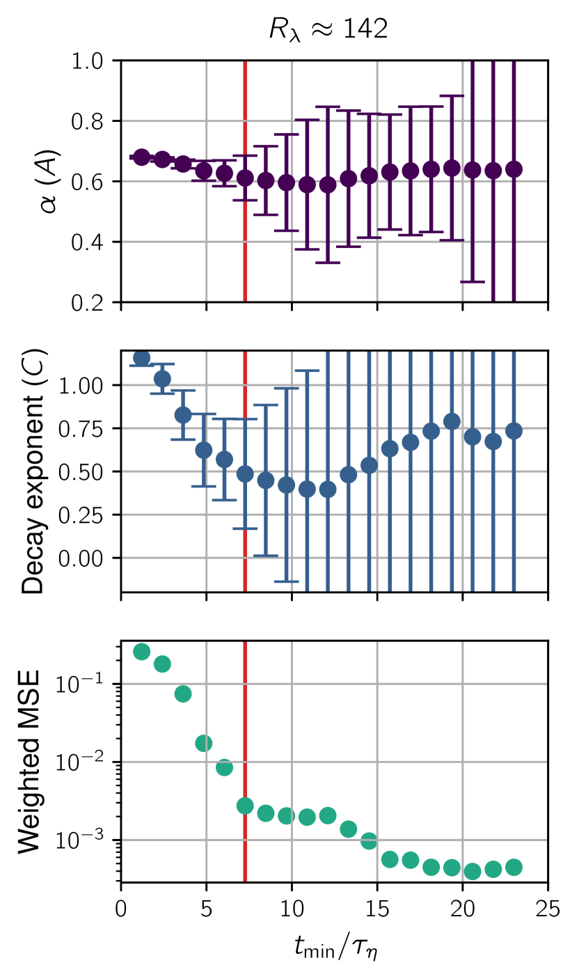
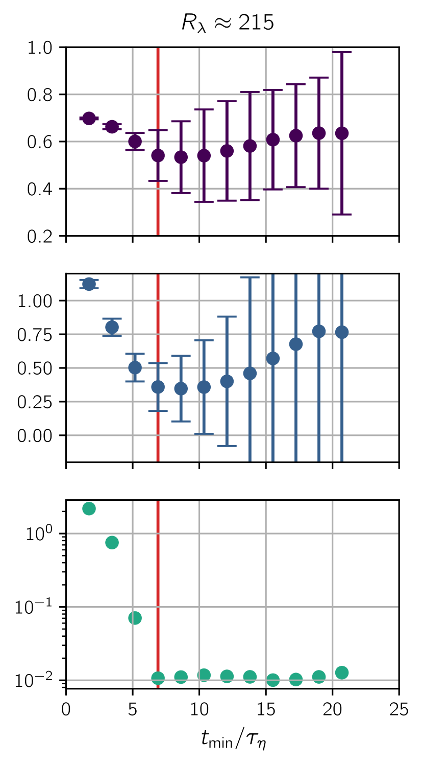
where A𝐴A, B𝐵B, and C𝐶C are fitting parameters. In order to robustly capture the asymptotic decay using this simple fit function, we leave out an initial transient regime of data points for the fit. We choose ttmin6.9τη𝑡subscript𝑡min6.9subscript𝜏𝜂t\geq t_{\mathrm{min}}\approx 6.9\tau_{\eta}, where the weighted mean squared error of the fit reaches a plateau, i.e. the point at which the fit improvement from removing more data points diminishes (for more details, see Supplementary Note 1). The parameters are estimated as A=0.54±0.11𝐴plus-or-minus0.540.11A=0.54\pm 0.11, B=(0.19±0.15)τη𝐵plus-or-minus0.190.15subscript𝜏𝜂B=(0.19\pm 0.15)\tau_{\eta} and C=0.36±0.18𝐶plus-or-minus0.360.18C=0.36\pm 0.18.

Note that the overall fitting procedure is very delicate and different choices may lead to different results. The present analysis is our best effort to systematically compute the limiting value of the minima.

Peak curvature dynamics of a parabola

Here, we determine the evolution of the peak curvature of a fold modeled by a parabola,

𝐋(ϕ,t)𝐋italic-ϕ𝑡\displaystyle\mathbf{L}(\phi,t) =𝐋(ϕ0,t)+(ϕϕ0)𝐥(t)Δsabsent𝐋subscriptitalic-ϕ0𝑡italic-ϕsubscriptitalic-ϕ0𝐥𝑡Δ𝑠\displaystyle=\mathbf{L}(\phi_{0},t)+(\phi-\phi_{0})\mathbf{l}(t)\Delta s (25)
+κp(0)(ϕϕ0)22𝐤(t)Δs2,subscript𝜅𝑝0superscriptitalic-ϕsubscriptitalic-ϕ022𝐤𝑡Δsuperscript𝑠2\displaystyle\quad+\kappa_{p}(0)\frac{(\phi-\phi_{0})^{2}}{2}\mathbf{k}(t)\Delta s^{2},

where ϕ0subscriptitalic-ϕ0\phi_{0} is the initial peak position, κp(0)subscript𝜅𝑝0\kappa_{p}(0) is its initial peak curvature, 𝐥𝐥\mathbf{l} and 𝐤𝐤\mathbf{k} are two initially orthonormal vectors, and ΔsΔ𝑠\Delta s is the arc length per angle of the initial parameterization at ϕ0subscriptitalic-ϕ0\phi_{0}. In a sufficiently small range of ϕitalic-ϕ\phi around ϕ0subscriptitalic-ϕ0\phi_{0}, the velocity field can be linearized. Then the parabolic shape is preserved and the dynamics of 𝐥𝐥\mathbf{l} and 𝐤𝐤\mathbf{k} in the Lagrangian frame is determined by the velocity gradient,

d𝐥dtd𝐥d𝑡\displaystyle\mathinner{\dfrac{\operatorname{d\!}{}\mathbf{l}}{\operatorname{d\!}{t}}} =𝐥𝐮(𝐋(ϕ0,t),t)andabsent𝐥𝐮𝐋subscriptitalic-ϕ0𝑡𝑡and\displaystyle=\mathbf{l}\cdot\nabla\mathbf{u}(\mathbf{L}(\phi_{0},t),t)\quad\text{and}
d𝐤dtd𝐤d𝑡\displaystyle\mathinner{\dfrac{\operatorname{d\!}{}\mathbf{k}}{\operatorname{d\!}{t}}} =𝐤𝐮(𝐋(ϕ0,t),t).absent𝐤𝐮𝐋subscriptitalic-ϕ0𝑡𝑡\displaystyle=\mathbf{k}\cdot\nabla\mathbf{u}(\mathbf{L}(\phi_{0},t),t). (26)

By (2), the curvature of the fold is given by

κ(ϕ,t)𝜅italic-ϕ𝑡\displaystyle\kappa(\phi,t) =κp(0)|𝐤(t)×𝐥(t)||𝐥(t)+Δs(ϕϕ0)κp(0)𝐤(t)|3absentsubscript𝜅𝑝0𝐤𝑡𝐥𝑡superscript𝐥𝑡Δ𝑠italic-ϕsubscriptitalic-ϕ0subscript𝜅𝑝0𝐤𝑡3\displaystyle=\kappa_{p}(0)\frac{\left|\mathbf{k}(t)\times\mathbf{l}(t)\right|}{\left|\mathbf{l}(t)+\Delta s(\phi-\phi_{0})\kappa_{p}(0)\mathbf{k}(t)\right|^{3}} (27)
=κp(0)(|𝐤(t)|2|𝐥(t)|2(𝐤(t)𝐥(t))2)1/2|𝐥(t)+Δs(ϕϕ0)κp(0)𝐤(t)|3.absentsubscript𝜅𝑝0superscriptsuperscript𝐤𝑡2superscript𝐥𝑡2superscript𝐤𝑡𝐥𝑡212superscript𝐥𝑡Δ𝑠italic-ϕsubscriptitalic-ϕ0subscript𝜅𝑝0𝐤𝑡3\displaystyle=\kappa_{p}(0)\frac{\left(\left|\mathbf{k}(t)\right|^{2}\left|\mathbf{l}(t)\right|^{2}-(\mathbf{k}(t)\cdot\mathbf{l}(t))^{2}\right)^{1/2}}{\left|\mathbf{l}(t)+\Delta s(\phi-\phi_{0})\kappa_{p}(0)\mathbf{k}(t)\right|^{3}}. (28)

Over time, 𝐥(t)𝐥𝑡\mathbf{l}(t) and 𝐤(t)𝐤𝑡\mathbf{k}(t) cease to be orthogonal and the curvature peak position is shifted. Minimizing the denominator yields the new peak position

ϕp(t)subscriptitalic-ϕ𝑝𝑡\displaystyle\phi_{p}(t) =ϕ0𝐤(t)𝐥(t)Δs|𝐤(t)|2κp(0).absentsubscriptitalic-ϕ0𝐤𝑡𝐥𝑡Δ𝑠superscript𝐤𝑡2subscript𝜅𝑝0\displaystyle=\phi_{0}-\frac{\mathbf{k}(t)\cdot\mathbf{l}(t)}{\Delta s\left|\mathbf{k}(t)\right|^{2}\kappa_{p}(0)}. (29)

The new peak curvature is therefore given by

κp(t):=κ(ϕp(t),t)=|𝐤(t)|3|𝐤(t)|2|𝐥(t)|2(𝐤(t)𝐥(t))2κp(0).\displaystyle\kappa_{p}(t)\mathrel{\mathop{\mathchar 58\relax}}=\kappa(\phi_{p}(t),t)=\frac{\left|\mathbf{k}(t)\right|^{3}}{\left|\mathbf{k}(t)\right|^{2}\left|\mathbf{l}(t)\right|^{2}-(\mathbf{k}(t)\cdot\mathbf{l}(t))^{2}}\kappa_{p}(0). (30)

Since 𝐥𝐥\mathbf{l} and 𝐤𝐤\mathbf{k} behave like passive vectors, their dynamics can be described by the deformation tensor

Fij(t)subscript𝐹𝑖𝑗𝑡\displaystyle F_{ij}(t) =Xi(𝐋(ϕ0,0),t)xj,absentsubscript𝑋𝑖𝐋subscriptitalic-ϕ00𝑡subscript𝑥𝑗\displaystyle=\mathinner{\dfrac{\partial{}X_{i}(\mathbf{L}(\phi_{0},0),t)}{\partial{x_{j}}}}, (31)

where 𝐗(𝐱,t)𝐗𝐱𝑡\mathbf{X}(\mathbf{x},t) is the Lagrangian map. The singular value decomposition of F𝐹F,

F(t)𝐹𝑡\displaystyle F(t) =U(t)Λ(t)VT(t),absent𝑈𝑡Λ𝑡superscript𝑉𝑇𝑡\displaystyle=U(t)\Lambda(t)V^{T}(t), (32)

defines the orthonormal bases (𝐮j(t))i=Uij(t)subscriptsubscript𝐮𝑗𝑡𝑖subscript𝑈𝑖𝑗𝑡(\mathbf{u}_{j}(t))_{i}=U_{ij}(t) and (𝐯j(t))i=Vij(t)subscriptsubscript𝐯𝑗𝑡𝑖subscript𝑉𝑖𝑗𝑡(\mathbf{v}_{j}(t))_{i}=V_{ij}(t) and the finite-time Lyapunov exponents ρi(t)subscript𝜌𝑖𝑡\rho_{i}(t) by Λii=eρi(t)tsubscriptΛ𝑖𝑖superscript𝑒subscript𝜌𝑖𝑡𝑡\Lambda_{ii}=e^{\rho_{i}(t)t} where ΛΛ\Lambda is diagonal. Expanding 𝐥(0)𝐥0\mathbf{l}(0) and 𝐤(0)𝐤0\mathbf{k}(0) in the 𝐯jsubscript𝐯𝑗\mathbf{v}_{j}-coordinate system yields

𝐥(0)𝐥0\displaystyle\mathbf{l}(0) =iai(t)𝐯i(t)andabsentsubscript𝑖subscript𝑎𝑖𝑡subscript𝐯𝑖𝑡and\displaystyle=\sum_{i}a_{i}(t)\mathbf{v}_{i}(t)\quad\text{and}
𝐤(0)𝐤0\displaystyle\mathbf{k}(0) =ibi(t)𝐯i(t).absentsubscript𝑖subscript𝑏𝑖𝑡subscript𝐯𝑖𝑡\displaystyle=\sum_{i}b_{i}(t)\mathbf{v}_{i}(t). (33)

Observing that F(t)𝐥(0)=𝐥(t)𝐹𝑡𝐥0𝐥𝑡F(t)\mathbf{l}(0)=\mathbf{l}(t) and F(t)𝐤(0)=𝐤(t)𝐹𝑡𝐤0𝐤𝑡F(t)\mathbf{k}(0)=\mathbf{k}(t), and applying the deformation tensor to the previous equations, we get

𝐥(t)𝐥𝑡\displaystyle\mathbf{l}(t) =iai(t)eρi(t)t𝐮i(t)andabsentsubscript𝑖subscript𝑎𝑖𝑡superscript𝑒subscript𝜌𝑖𝑡𝑡subscript𝐮𝑖𝑡and\displaystyle=\sum_{i}a_{i}(t)e^{\rho_{i}(t)t}\mathbf{u}_{i}(t)\quad\text{and}
𝐤(t)𝐤𝑡\displaystyle\mathbf{k}(t) =ibi(t)eρi(t)t𝐮i(t).absentsubscript𝑖subscript𝑏𝑖𝑡superscript𝑒subscript𝜌𝑖𝑡𝑡subscript𝐮𝑖𝑡\displaystyle=\sum_{i}b_{i}(t)e^{\rho_{i}(t)t}\mathbf{u}_{i}(t). (34)

Inserting these expansions into (30) yields

κp(t)=(ibi2e2ρit)3/2ijajbi(ajbiaibj)e(2ρi+2ρj)tκp(0).subscript𝜅𝑝𝑡superscriptsubscript𝑖superscriptsubscript𝑏𝑖2superscript𝑒2subscript𝜌𝑖𝑡32subscript𝑖𝑗subscript𝑎𝑗subscript𝑏𝑖subscript𝑎𝑗subscript𝑏𝑖subscript𝑎𝑖subscript𝑏𝑗superscript𝑒2subscript𝜌𝑖2subscript𝜌𝑗𝑡subscript𝜅𝑝0\displaystyle\kappa_{p}(t)=\frac{\left(\sum_{i}b_{i}^{2}e^{2\rho_{i}t}\right)^{3/2}}{\sum_{i\neq j}a_{j}b_{i}(a_{j}b_{i}-a_{i}b_{j})e^{(2\rho_{i}+2\rho_{j})t}}\kappa_{p}(0). (35)

As long as the infinite-time Lyapunov exponents (the t𝑡t\to\infty-limits of the FTLEs) are distinct from each other, we will have eρ1(t)teρ2(t)teρ3(t)tmuch-greater-thansuperscript𝑒subscript𝜌1𝑡𝑡superscript𝑒subscript𝜌2𝑡𝑡much-greater-thansuperscript𝑒subscript𝜌3𝑡𝑡e^{\rho_{1}(t)t}\gg e^{\rho_{2}(t)t}\gg e^{\rho_{3}(t)t} for large t𝑡t. Assuming furthermore that the random coefficients in (35) are non-zero, we can drop those terms with slower exponential growth:

κp(t)t0|b1(t)|3(a2(t)b1(t)a1(t)b2(t))2κp(0)e[ρ1(t)2ρ2(t)]t.superscriptmuch-greater-than𝑡0subscript𝜅𝑝𝑡superscriptsubscript𝑏1𝑡3superscriptsubscript𝑎2𝑡subscript𝑏1𝑡subscript𝑎1𝑡subscript𝑏2𝑡2subscript𝜅𝑝0superscript𝑒delimited-[]subscript𝜌1𝑡2subscript𝜌2𝑡𝑡\displaystyle\kappa_{p}(t)\stackrel{{\scriptstyle t\gg 0}}{{\approx}}\frac{|b_{1}(t)|^{3}}{(a_{2}(t)b_{1}(t)-a_{1}(t)b_{2}(t))^{2}}\kappa_{p}(0)e^{[\rho_{1}(t)-2\rho_{2}(t)]t}. (36)

While the FTLEs are known to converge slowly, V(t)𝑉𝑡V(t) and thus ai(t)subscript𝑎𝑖𝑡a_{i}(t) and bi(t)subscript𝑏𝑖𝑡b_{i}(t) converge exponentially fast [56, 57]. We therefore have (cf. ref. [32])

κp(t)t0κ~0e[ρ1(t)2ρ2(t)]t,superscriptmuch-greater-than𝑡0subscript𝜅𝑝𝑡subscript~𝜅0superscript𝑒delimited-[]subscript𝜌1𝑡2subscript𝜌2𝑡𝑡\displaystyle\kappa_{p}(t)\stackrel{{\scriptstyle t\gg 0}}{{\approx}}\widetilde{\kappa}_{0}e^{[\rho_{1}(t)-2\rho_{2}(t)]t}, (37)

for some effective initial peak curvature

κ~0=limt|b1(t)|3(a2(t)b1(t)a1(t)b2(t))2κp(0),subscript~𝜅0subscript𝑡superscriptsubscript𝑏1𝑡3superscriptsubscript𝑎2𝑡subscript𝑏1𝑡subscript𝑎1𝑡subscript𝑏2𝑡2subscript𝜅𝑝0\displaystyle\widetilde{\kappa}_{0}=\lim_{t\to\infty}\frac{|b_{1}(t)|^{3}}{(a_{2}(t)b_{1}(t)-a_{1}(t)b_{2}(t))^{2}}\kappa_{p}(0), (38)

which may differ from the actual initial peak curvature κp(0)subscript𝜅𝑝0\kappa_{p}(0) depending on the relative orientation of the initial parabola and the converged basis vectors limt𝐯j(t)subscript𝑡subscript𝐯𝑗𝑡\lim_{t\to\infty}\mathbf{v}_{j}(t).

Extracting the power law by the method of steepest descent

In order to extract the asymptotic regime of the integral (14), we substitute the integration variable

ρp=1τlog(κpκ0),subscript𝜌𝑝1𝜏subscript𝜅𝑝subscript𝜅0\displaystyle\rho_{p}=\frac{1}{\tau}\log\left(\frac{\kappa_{p}}{\kappa_{0}}\right), (39)

which yields

f(κp)1κp0dρpN(log(κp/κ0)/ρp)ρpelog(κpκ0)(β+S(ρp))ρp.similar-to𝑓subscript𝜅𝑝1subscript𝜅𝑝superscriptsubscript0dsubscript𝜌𝑝𝑁subscript𝜅𝑝subscript𝜅0subscript𝜌𝑝subscript𝜌𝑝superscript𝑒subscript𝜅𝑝subscript𝜅0𝛽𝑆subscript𝜌𝑝subscript𝜌𝑝\displaystyle f(\kappa_{p})\sim\frac{1}{\kappa_{p}}\int_{0}^{\infty}\operatorname{d\!}\rho_{p}\frac{N(\log(\kappa_{p}/\kappa_{0})/\rho_{p})}{\rho_{p}}e^{-\log\left(\frac{\kappa_{p}}{\kappa_{0}}\right)\frac{(\beta+S(\rho_{p}))}{\rho_{p}}}. (40)

We now explore the regime where log(κp/κ0)subscript𝜅𝑝subscript𝜅0\log(\kappa_{p}/\kappa_{0}) becomes large. Assuming that the normalization function N(τ)𝑁𝜏N(\tau) is algebraic, the scaling of the integral with κpsubscript𝜅𝑝\kappa_{p} is dominated by the exponential, and in particular by the part that has the slowest decay. To first order, we therefore have [41, Chapter 9, Theorem 2.1]

f(κp)𝑓subscript𝜅𝑝\displaystyle f(\kappa_{p}) 1κpexp(log(κpκ0)minρp[1ρp(β+S(ρp))])similar-toabsent1subscript𝜅𝑝subscript𝜅𝑝subscript𝜅0subscriptsubscript𝜌𝑝1subscript𝜌𝑝𝛽𝑆subscript𝜌𝑝\displaystyle\sim\frac{1}{\kappa_{p}}\exp\left(-\log\left(\frac{\kappa_{p}}{\kappa_{0}}\right)\min_{\rho_{p}}\left[\tfrac{1}{\rho_{p}}(\beta+S(\rho_{p}))\right]\right)
κp1α,proportional-toabsentsuperscriptsubscript𝜅𝑝1𝛼\displaystyle\propto\kappa_{p}^{-1-\alpha}, (41)

with

α=minρp[1ρp(β+S(ρp))].𝛼subscriptsubscript𝜌𝑝1subscript𝜌𝑝𝛽𝑆subscript𝜌𝑝\displaystyle\alpha=\min_{\rho_{p}}\left[\tfrac{1}{\rho_{p}}(\beta+S(\rho_{p}))\right]. (42)

Relating our results to generalized Lyapunov exponents

Let us define a generalized Lyapunov exponent of curvature peaks by

Lp(q)subscript𝐿𝑝𝑞\displaystyle L_{p}(q) =limt1tlogexp(qρp(t)t).absentsubscript𝑡1𝑡𝑞subscript𝜌𝑝𝑡𝑡\displaystyle=\lim_{t\to\infty}\frac{1}{t}\log\left\langle\exp(q\rho_{p}(t)t)\right\rangle. (43)

It differs from the usual definition of generalized Lyapunov exponents only by the fact that we have replaced the standard FTLE by our curvature peak FTLE ρp(t)=ρ1(t)2ρ2(t)subscript𝜌𝑝𝑡subscript𝜌1𝑡2subscript𝜌2𝑡\rho_{p}(t)=\rho_{1}(t)-2\rho_{2}(t). It is related to the Cramér function by a Legendre transform [39],

Lp(q)subscript𝐿𝑝𝑞\displaystyle L_{p}(q) =supρp[qρpS(ρp)].absentsubscriptsupremumsubscript𝜌𝑝delimited-[]𝑞subscript𝜌𝑝𝑆subscript𝜌𝑝\displaystyle=\sup_{\rho_{p}}\left[q\rho_{p}-S(\rho_{p})\right]. (44)

This strongly resembles our steepest-descent formula established in the main text (cf. (15)),

α𝛼\displaystyle\alpha =minρp[1ρp(β+S(ρp))]absentsubscriptsubscript𝜌𝑝1subscript𝜌𝑝𝛽𝑆subscript𝜌𝑝\displaystyle=\min_{\rho_{p}}\left[\tfrac{1}{\rho_{p}}(\beta+S(\rho_{p}))\right] (45)

where, recall, β𝛽\beta is identified with line growth quantified by the first FTLE (see Fig. 3 and subsequent discussion)

β=limt1tlogexp(ρ1(t)t).𝛽subscript𝑡1𝑡subscript𝜌1𝑡𝑡\displaystyle\beta=\lim_{t\to\infty}\frac{1}{t}\log\left\langle\exp(\rho_{1}(t)t)\right\rangle. (46)

We claim Lp(α)=βsubscript𝐿𝑝𝛼𝛽L_{p}(\alpha)=\beta. If so, then equating (43) evaluated at α𝛼\alpha with β𝛽\beta given by (46), we find

limt1tlogexp(αρp(t)t)subscript𝑡1𝑡𝛼subscript𝜌𝑝𝑡𝑡\displaystyle\lim_{t\to\infty}\frac{1}{t}\log\left\langle\exp(\alpha\rho_{p}(t)t)\right\rangle =limt1tlogexp(ρ1(t)t),absentsubscript𝑡1𝑡subscript𝜌1𝑡𝑡\displaystyle=\lim_{t\to\infty}\frac{1}{t}\log\left\langle\exp(\rho_{1}(t)t)\right\rangle, (47)

which we write in short form as (17).

To verify that Lp(α)=βsubscript𝐿𝑝𝛼𝛽L_{p}(\alpha)=\beta, we insert α𝛼\alpha into (44) to find

Lp(α)=supρp[αρpS(ρp)].subscript𝐿𝑝𝛼subscriptsupremumsubscript𝜌𝑝delimited-[]𝛼subscript𝜌𝑝𝑆subscript𝜌𝑝\displaystyle L_{p}(\alpha)=\sup_{\rho_{p}}\left[\alpha\rho_{p}-S(\rho_{p})\right]. (48)

Assuming that S(ρp)𝑆subscript𝜌𝑝S(\rho_{p}) is differentiable and strictly convex, the supremum in (48) occurs at a unique value ρpsuperscriptsubscript𝜌𝑝\rho_{p}^{*}. Moreover, somewhat remarkably, we will show that this value coincides with that at which the minimum of (45) occurs. Once established, this gives the claimed result upon substitution of α=1ρp(β+S(ρp))𝛼1superscriptsubscript𝜌𝑝𝛽𝑆superscriptsubscript𝜌𝑝\alpha=\tfrac{1}{\rho_{p}^{*}}(\beta+S(\rho_{p}^{*})) into Lp(α)=αρpS(ρp)subscript𝐿𝑝𝛼𝛼superscriptsubscript𝜌𝑝𝑆superscriptsubscript𝜌𝑝L_{p}(\alpha)=\alpha\rho_{p}^{*}-S(\rho_{p}^{*}).

To see that the extrema in (48) and (45) occur at the same point ρpsuperscriptsubscript𝜌𝑝\rho_{p}^{*}, we note that under our assumptions (48) is minimized at the ρ=ρ𝜌superscript𝜌\rho=\rho^{*} for which

00\displaystyle 0 =ddρ[αρS(ρ)]|ρ=ρ=αS(ρ).absentevaluated-atdd𝜌delimited-[]𝛼𝜌𝑆𝜌𝜌superscript𝜌𝛼superscript𝑆superscript𝜌\displaystyle=\mathinner{\dfrac{\operatorname{d\!}{}}{\operatorname{d\!}{\rho}}}\left[\alpha\rho-S(\rho)\right]\Big{|}_{\rho=\rho^{*}}=\alpha-S^{\prime}(\rho^{*}). (49)

Uniqueness follows from our assumption that S(ρ)superscript𝑆𝜌S^{\prime}(\rho) is an invertible function of ρ𝜌\rho. On the other hand, the minimum in (45) occurs for ρ=ρ𝜌superscript𝜌absent\rho=\rho^{**} satisfying

00\displaystyle 0 =ddρ[1ρ(β+S(ρ))]|ρ=ρabsentevaluated-atdd𝜌delimited-[]1𝜌𝛽𝑆𝜌𝜌superscript𝜌absent\displaystyle=\mathinner{\dfrac{\operatorname{d\!}{}}{\operatorname{d\!}{\rho}}}\left[\tfrac{1}{\rho}(\beta+S(\rho))\right]\Big{|}_{\rho=\rho^{**}}
=1ρ(1ρ(β+S(ρ))S(ρ))absent1superscript𝜌absent1superscript𝜌absent𝛽𝑆superscript𝜌absentsuperscript𝑆superscript𝜌absent\displaystyle=-\frac{1}{\rho^{**}}\left(\tfrac{1}{\rho^{**}}(\beta+S(\rho^{**}))-S^{\prime}(\rho^{**})\right)
=1ρ(αS(ρ))absent1superscript𝜌absent𝛼superscript𝑆superscript𝜌absent\displaystyle=-\frac{1}{\rho^{**}}\left(\alpha-S^{\prime}(\rho^{**})\right) (50)

where we have inserted the expression for α𝛼\alpha in terms of the minimizing argument ρsuperscript𝜌absent\rho^{**} given by (45). It is clear from comparing (49) and (50) that the extrema are realized at the same value ρ=ρ=:ρp\rho^{*}=\rho^{**}=\mathrel{\mathop{\mathchar 58\relax}}\rho^{*}_{p}. This concludes the proof.

Fokker-Planck equation of curvature in the Kraichnan model

In the Kraichnan model, the velocity field 𝐮(𝐱,t)𝐮𝐱𝑡\mathbf{u}(\mathbf{x},t) is Gaussian with correlation tensor

ui(𝐱,t)uj(𝐱,t)delimited-⟨⟩subscript𝑢𝑖𝐱𝑡subscript𝑢𝑗superscript𝐱superscript𝑡\displaystyle\left\langle u_{i}(\mathbf{x},t)u_{j}(\mathbf{x}^{\prime},t^{\prime})\right\rangle =δ(tt)Rij(𝐱𝐱),absent𝛿𝑡superscript𝑡subscript𝑅𝑖𝑗𝐱superscript𝐱\displaystyle=\delta(t-t^{\prime})R_{ij}(\mathbf{x}-\mathbf{x}^{\prime}), (51)

where Rij(𝐫)subscript𝑅𝑖𝑗𝐫R_{ij}(\mathbf{r}) denotes the spatial part of the correlation tensor.

Equivalent to (3), the curvature PDF weighted by arc length can be defined by

f(κ;t)=|ϕ𝐋|δ(κκ~(ϕ,t))|ϕ𝐋|,𝑓𝜅𝑡delimited-⟨⟩subscriptitalic-ϕ𝐋𝛿𝜅~𝜅italic-ϕ𝑡delimited-⟨⟩subscriptitalic-ϕ𝐋f(\kappa;t)=\frac{\left\langle|\partial_{\phi}\mathbf{L}|\delta(\kappa-\tilde{\kappa}(\phi,t))\right\rangle}{\left\langle|\partial_{\phi}\mathbf{L}|\right\rangle}, (52)

where we distinguish between the realization κ~~𝜅\tilde{\kappa} and the sample-space variable κ𝜅\kappa. Angular brackets delimited-⟨⟩\langle\cdot\rangle denote an average along ϕitalic-ϕ\phi and over realizations of the velocity field.

In order to derive the Fokker-Planck equation of curvature, we take the time derivative of (52), which yields

tf(κ;t)subscript𝑡𝑓𝜅𝑡\displaystyle\partial_{t}f(\kappa;t) =δ(κκ~)t|ϕ𝐋||ϕ𝐋|f(κ;t)t|ϕ𝐋||ϕ𝐋|absentdelimited-⟨⟩𝛿𝜅~𝜅subscript𝑡subscriptitalic-ϕ𝐋delimited-⟨⟩subscriptitalic-ϕ𝐋𝑓𝜅𝑡subscript𝑡delimited-⟨⟩subscriptitalic-ϕ𝐋delimited-⟨⟩subscriptitalic-ϕ𝐋\displaystyle=\frac{\left\langle\delta(\kappa-\tilde{\kappa})\partial_{t}|\partial_{\phi}\mathbf{L}|\right\rangle}{\left\langle|\partial_{\phi}\mathbf{L}|\right\rangle}-f(\kappa;t)\frac{\partial_{t}\left\langle|\partial_{\phi}\mathbf{L}|\right\rangle}{\left\langle|\partial_{\phi}\mathbf{L}|\right\rangle} (53)
1|ϕ𝐋|κδ(κκ~)|ϕ𝐋|tκ~.1delimited-⟨⟩subscriptitalic-ϕ𝐋subscript𝜅quantum-operator-product𝛿𝜅~𝜅subscriptitalic-ϕ𝐋subscript𝑡~𝜅\displaystyle\quad-\frac{1}{\left\langle|\partial_{\phi}\mathbf{L}|\right\rangle}\partial_{\kappa}\left\langle\delta(\kappa-\tilde{\kappa})|\partial_{\phi}\mathbf{L}|\partial_{t}\tilde{\kappa}\right\rangle.

The averages can be evaluated using the Gaussian integration by parts formula [58, 59, 60] and the evolution equations [22]

tϕ𝐋subscript𝑡subscriptitalic-ϕ𝐋\displaystyle\partial_{t}\partial_{\phi}\mathbf{L} =((ϕ𝐋))𝐮,absentsubscriptitalic-ϕ𝐋𝐮\displaystyle=((\partial_{\phi}\mathbf{L})\cdot\nabla)\mathbf{u}, (54)
t𝐭^subscript𝑡^𝐭\displaystyle\partial_{t}\hat{\mathbf{t}} =(𝐭^)𝐮𝐭^(𝐭^(𝐭^)𝐮),absent^𝐭𝐮^𝐭^𝐭^𝐭𝐮\displaystyle=(\hat{\mathbf{t}}\cdot\nabla)\mathbf{u}-\hat{\mathbf{t}}(\hat{\mathbf{t}}\cdot(\hat{\mathbf{t}}\cdot\nabla)\mathbf{u}), (55)
t𝐧^subscript𝑡^𝐧\displaystyle\partial_{t}\hat{\mathbf{n}} =𝐛^(𝐛^(𝐧^)𝐮)𝐭^(𝐧^(𝐭^)𝐮)absent^𝐛^𝐛^𝐧𝐮^𝐭^𝐧^𝐭𝐮\displaystyle=\hat{\mathbf{b}}(\hat{\mathbf{b}}\cdot(\hat{\mathbf{n}}\cdot\nabla)\mathbf{u})-\hat{\mathbf{t}}(\hat{\mathbf{n}}\cdot(\hat{\mathbf{t}}\cdot\nabla)\mathbf{u})
+1κ~𝐛^(𝐛^(𝐭^)2𝐮),1~𝜅^𝐛^𝐛superscript^𝐭2𝐮\displaystyle\quad\ \ +\frac{1}{\tilde{\kappa}}\hat{\mathbf{b}}(\hat{\mathbf{b}}\cdot(\hat{\mathbf{t}}\cdot\nabla)^{2}\mathbf{u}), (56)
tκ~subscript𝑡~𝜅\displaystyle\partial_{t}\tilde{\kappa} =κ~(𝐧^(𝐧^)𝐮2𝐭^(𝐭^)𝐮)absent~𝜅^𝐧^𝐧𝐮2^𝐭^𝐭𝐮\displaystyle=\tilde{\kappa}\left(\hat{\mathbf{n}}\cdot(\hat{\mathbf{n}}\cdot\nabla)\mathbf{u}-2\hat{\mathbf{t}}\cdot(\hat{\mathbf{t}}\cdot\nabla)\mathbf{u}\right)
+𝐧^(𝐭^)2𝐮.^𝐧superscript^𝐭2𝐮\displaystyle\quad\ \ +\hat{\mathbf{n}}\cdot(\hat{\mathbf{t}}\cdot\nabla)^{2}\mathbf{u}. (57)

Here, 𝐭^^𝐭\hat{\mathbf{t}}, 𝐧^^𝐧\hat{\mathbf{n}} and 𝐛^^𝐛\hat{\mathbf{b}} denote the tangent, normal and binormal vector of the Frenet-Serret frame, respectively. As shown in Supplementary Note 5, the evolution equations derive from the definitions of the various quantities combined with the tracer equation (1). All quantities are evaluated along the same Lagrangian trajectory.

In order to simplify the resulting expressions, we need to further restrict the spatial correlation structure of the model. Isotropy and incompressibility determine the form of the even derivatives of the spatial correlation tensor Rij(𝐫)subscript𝑅𝑖𝑗𝐫R_{ij}(\mathbf{r}) at 𝟎0\mathbf{0} (odd numbers of derivatives vanish) to be [61]

klRij(𝟎)subscript𝑘subscript𝑙subscript𝑅𝑖𝑗0\displaystyle-\partial_{k}\partial_{l}R_{ij}(\mathbf{0}) =Q(4δijδklδikδjlδilδjk)absent𝑄4subscript𝛿𝑖𝑗subscript𝛿𝑘𝑙subscript𝛿𝑖𝑘subscript𝛿𝑗𝑙subscript𝛿𝑖𝑙subscript𝛿𝑗𝑘\displaystyle=Q(4\delta_{ij}\delta_{kl}-\delta_{ik}\delta_{jl}-\delta_{il}\delta_{jk}) (58)

and [62]

klmnRij(𝟎)subscript𝑘subscript𝑙subscript𝑚subscript𝑛subscript𝑅𝑖𝑗0\displaystyle\partial_{k}\partial_{l}\partial_{m}\partial_{n}R_{ij}(\mathbf{0}) =P(6δijδklδmn+6δijδkmδln\displaystyle=P(6\delta_{ij}\delta_{kl}\delta_{mn}+6\delta_{ij}\delta_{km}\delta_{ln} (59)
+6δijδknδlm(all others)),\displaystyle\quad+6\delta_{ij}\delta_{kn}\delta_{lm}-(\text{all others})),

with Q𝑄Q and P𝑃P scalar constants that depend on the exact form of Rij(𝐫)subscript𝑅𝑖𝑗𝐫R_{ij}(\mathbf{r}). The last pair of brackets contains all twelve other permutations of Kronecker deltas. All terms arising from the Gaussian integration by parts formula can be evaluated using this result and the orthonormality of the Frenet-Serret frame. The resulting Fokker-Planck equation is (20). In Supplementary Note 6, we list results for all terms and exemplify computing one of them.

\EdefEscapeHexData availability.1Data availability.1\EdefEscapeHexData availabilityData availability\hyper@anchorstartData availability.1\hyper@anchorendData availability

The data that support the findings of this study are available from the corresponding author upon reasonable request.

\EdefEscapeHexCode availability.1Code availability.1\EdefEscapeHexCode availabilityCode availability\hyper@anchorstartCode availability.1\hyper@anchorendCode availability

The simulation results have been generated with our code TurTLE [48], which is available on https://gitlab.mpcdf.mpg.de/TurTLE/turtle. The loop refinement and post-processing codes are available from the corresponding author upon reasonable request.

References

  • Dimotakis [2005] P. E. Dimotakis, Turbulent mixing, Annu. Rev. Fluid Mech. 37, 329 (2005).
  • Prants et al. [2014] S. Prants, M. Budyansky, and M. Uleysky, Identifying Lagrangian fronts with favourable fishery conditions, Deep Sea Res. Part I 90, 27 (2014).
  • Haynes and McIntyre [1987] P. H. Haynes and M. E. McIntyre, On the evolution of vorticity and potential vorticity in the presence of diabatic heating and frictional or other forces, J. Atmos. Sci. 44, 828 (1987).
  • Ohkitani [2002] K. Ohkitani, Numerical study of comparison of vorticity and passive vectors in turbulence and inviscid flows, Phys. Rev. E 65, 046304 (2002).
  • Guala et al. [2005] M. Guala, B. Lüthi, A. Liberzon, A. Tsinober, and W. Kinzelbach, On the evolution of material lines and vorticity in homogeneous turbulence, J. Fluid Mech. 533, 339 (2005).
  • Balkovsky et al. [2000] E. Balkovsky, A. Fouxon, and V. Lebedev, Turbulent dynamics of polymer solutions, Phys. Rev. Lett. 84, 4765 (2000).
  • Liberzon et al. [2005] A. Liberzon, M. Guala, B. Lüthi, W. Kinzelbach, and A. Tsinober, Turbulence in dilute polymer solutions, Phys. Fluids 17, 031707 (2005).
  • Bagheri et al. [2012] F. Bagheri, D. Mitra, P. Perlekar, and L. Brandt, Statistics of polymer extensions in turbulent channel flow, Phys. Rev. E 86, 056314 (2012).
  • Musielak et al. [2009] M. M. Musielak, L. Karp-Boss, P. A. Jumars, and L. J. Fauci, Nutrient transport and acquisition by diatom chains in a moving fluid, J. Fluid Mech. 638, 401 (2009).
  • Davidson [2013] P. A. Davidson, Turbulence in Rotating, Stratified and Electrically Conducting Fluids (Cambridge University Press, Cambridge, 2013).
  • Batchelor and Taylor [1952] G. K. Batchelor and G. I. Taylor, The effect of homogeneous turbulence on material lines and surfaces, Proc. R. Soc. Lond. A 213, 349 (1952).
  • Girimaji and Pope [1990] S. S. Girimaji and S. B. Pope, Material-element deformation in isotropic turbulence, J. Fluid Mech. 220, 427 (1990).
  • Drummond and Münch [1990] I. T. Drummond and W. Münch, Turbulent stretching of line and surface elements, J. Fluid Mech. 215, 45 (1990).
  • Ishihara and Kaneda [1992] T. Ishihara and Y. Kaneda, Stretching and distortion of material line elements in two-dimensional turbulence, J. Phys. Soc. Jpn. 61, 3547 (1992).
  • Tabor and Klapper [1994] M. Tabor and I. Klapper, Stretching and alignment in chaotic and turbulent flows, Chaos Soliton. Fract. 4, 1031 (1994).
  • Villermaux and Gagne [1994] E. Villermaux and Y. Gagne, Line dispersion in homogeneous turbulence: Stretching, fractal dimensions, and micromixing, Phys. Rev. Lett. 73, 252 (1994).
  • Nicolleau [1996] F. Nicolleau, Numerical determination of turbulent fractal dimensions, Phys. Fluids 8, 2661 (1996).
  • Iyer et al. [2020] K. P. Iyer, J. Schumacher, K. R. Sreenivasan, and P. K. Yeung, Fractal iso-level sets in high-Reynolds-number scalar turbulence, Phys. Rev. Fluids 5, 044501 (2020).
  • Bär [2010] C. Bär, Elementary Differential Geometry (Cambridge University Press, 2010).
  • Pope [1988] S. B. Pope, The evolution of surfaces in turbulence, Int. J. Eng. Sci. 26, 445 (1988).
  • Pope et al. [1989] S. B. Pope, P. K. Yeung, and S. S. Girimaji, The curvature of material surfaces in isotropic turbulence, Phys. Fluids A 1, 2010 (1989).
  • Drummond and Münch [1991] I. T. Drummond and W. Münch, Distortion of line and surface elements in model turbulent flows, J. Fluid Mech. 225, 529 (1991).
  • Girimaji [1991] S. Girimaji, Asymptotic behavior of curvature of surface elements in isotropic turbulence, Phys. Fluids A 3, 1772 (1991).
  • Drummond [1993] I. T. Drummond, Stretching and bending of line elements in random flows, J. Fluid Mech. 252, 479 (1993).
  • Liu and Muzzio [1996] M. Liu and F. Muzzio, The curvature of material lines in chaotic cavity flows, Phys. Fluids 8, 75 (1996).
  • Hobbs et al. [1997] D. M. Hobbs, M. M. Alvarez, and F. J. Muzzio, Mixing in globally chaotic flows, Fractals 5, 395 (1997).
  • Hobbs and Muzzio [1998] D. M. Hobbs and F. J. Muzzio, The curvature of material lines in a three-dimensional chaotic flow, Phys. Fluids 10, 1942 (1998).
  • Cerbelli et al. [2000] S. Cerbelli, J. M. Zalc, and F. J. Muzzio, The evolution of material lines curvature in deterministic chaotic flows, Chem. Eng. Sci. 55, 363 (2000).
  • Kivotides [2003] D. Kivotides, Geometry of turbulent tangles of material lines, Phys. Lett. A 318, 574 (2003).
  • Thiffeault [2004] J.-L. Thiffeault, Stretching and curvature of material lines in chaotic flows, Physica D 198, 169 (2004).
  • Leonard [2005] A. Leonard, Curvature and torsion of material lines in chaotic flows, Fluid Dyn. Res. 36, 261 (2005).
  • Leonard [2009] A. Leonard, The universal structure of high-curvature regions of material lines in chaotic flows, J. Fluid Mech. 622, 167 (2009).
  • Thiffeault et al. [2009] J.-L. Thiffeault, E. Gouillart, and M. D. Finn, The size of ghost rods, in Analysis and Control of Mixing with an Application to Micro and Macro Flow Processes, edited by L. Cortelezzi and I. Mezić (Springer Vienna, Vienna, 2009) pp. 339–350.
  • Ma and Bollt [2014] T. Ma and E. M. Bollt, Differential geometry perspective of shape coherence and curvature evolution by finite-time nonhyperbolic splitting, SIAM J. Appl. Dyn. Syst. 13, 1106 (2014).
  • Braun et al. [2006] W. Braun, F. De Lillo, and B. Eckhardt, Geometry of particle paths in turbulent flows, J. Turbul. 7, N62 (2006).
  • Xu et al. [2007] H. Xu, N. T. Ouellette, and E. Bodenschatz, Curvature of Lagrangian trajectories in turbulence, Phys. Rev. Lett. 98, 050201 (2007).
  • Scagliarini [2011] A. Scagliarini, Geometric properties of particle trajectories in turbulent flows, J. Turbul. 12, N25 (2011).
  • Bec et al. [2006] J. Bec, L. Biferale, G. Boffetta, M. Cencini, S. Musacchio, and F. Toschi, Lyapunov exponents of heavy particles in turbulence, Phys. Fluids 18, 091702 (2006).
  • Johnson and Meneveau [2015] P. L. Johnson and C. Meneveau, Large-deviation joint statistics of the finite-time Lyapunov spectrum in isotropic turbulence, Phys. Fluids 27, 085110 (2015).
  • Balkovsky and Fouxon [1999] E. Balkovsky and A. Fouxon, Universal long-time properties of Lagrangian statistics in the Batchelor regime and their application to the passive scalar problem, Phys. Rev. E 60, 4164 (1999).
  • Olver [1997] F. W. J. Olver, Asymptotics and Special Functions (A K Peters, 1997).
  • Kraichnan [1968] R. H. Kraichnan, Small-scale structure of a scalar field convected by turbulence, Phys. Fluids 11, 945 (1968).
  • Schekochihin et al. [2001] A. Schekochihin, S. Cowley, J. Maron, and L. Malyshkin, Structure of small-scale magnetic fields in the kinematic dynamo theory, Phys. Rev. E 65, 016305 (2001).
  • Cardy et al. [2008] J. Cardy, G. Falkovich, and K. Gawedzki, Non-equilibrium Statistical Mechanics and Turbulence, edited by S. Nazarenko and O. V. Zaboronski, London Mathematical Society Lecture Note Series (Cambridge University Press, 2008).
  • Childress and Gilbert [1995] S. Childress and A. D. Gilbert, Stretch, Twist, Fold: The Fast Dynamo, Vol. 37 (Springer Science & Business Media, 1995).
  • Ott [1998] E. Ott, Chaotic flows and kinematic magnetic dynamos: a tutorial review, Phys. Plasmas 5, 1636 (1998).
  • Boozer [1993] A. H. Boozer, Magnetic helicity and dynamos, Phys. Fluids B: Plasma Physics 5, 2271 (1993).
  • Lalescu et al. [2021] C. C. Lalescu, B. Bramas, M. Rampp, and M. Wilczek, An efficient particle tracking algorithm for large-scale parallel pseudo-spectral simulations of turbulence (2021), arXiv:2107.01104 [physics.flu-dyn] .
  • Hou and Li [2007] T. Y. Hou and R. Li, Computing nearly singular solutions using pseudo-spectral methods, J. Comput. Phys. 226, 379 (2007).
  • Kida and Goto [2002] S. Kida and S. Goto, Line statistics: Stretching rate of passive lines in turbulence, Phys. Fluids 14, 352 (2002).
  • Goto and Kida [2007] S. Goto and S. Kida, Reynolds-number dependence of line and surface stretching in turbulence: folding effects, J. Fluid Mech. 586, 59 (2007).
  • Virtanen et al. [2020] P. Virtanen et al., SciPy 1.0: fundamental algorithms for scientific computing in Python, Nat. Methods 17, 261 (2020).
  • Lalescu et al. [2010] C. C. Lalescu, B. Teaca, and D. Carati, Implementation of high order spline interpolations for tracking test particles in discretized fields, J. Comput. Phys. 229, 5862 (2010).
  • Eyink [2006] G. L. Eyink, Turbulent cascade of circulations, C. R. Phys. 7, 449 (2006).
  • Pikovsky and Politi [2016] A. Pikovsky and A. Politi, Lyapunov Exponents: A Tool to Explore Complex Dynamics (Cambridge University Press, 2016).
  • Thiffeault [2002] J.-L. Thiffeault, Derivatives and constraints in chaotic flows: asymptotic behaviour and a numerical method, Physica D 172, 139 (2002).
  • Goldhirsch et al. [1987] I. Goldhirsch, P.-L. Sulem, and S. A. Orszag, Stability and Lyapunov stability of dynamical systems: A differential approach and a numerical method, Physica D 27, 311 (1987).
  • Furutsu [1964] K. Furutsu, On the Statistical Theory of Electromagnetic Waves in a Fluctuating Medium (II), NBS Monograph No. 79 (U.S. Natl. Inst. Stand., 1964).
  • Donsker [1967] M. D. Donsker, On function space integrals, Matematika 11, 128 (1967).
  • Novikov [1965] E. A. Novikov, Functionals and the random-force method in turbulence theory, Sov. J. Exp. Theor. Phys. 20, 1290 (1965).
  • Pumir [2017] A. Pumir, Structure of the velocity gradient tensor in turbulent shear flows, Phys. Rev. Fluids 2, 074602 (2017).
  • Kearsley and Fong [1975] E. A. Kearsley and J. T. Fong, Linearly independent sets of isotropic Cartesian tensors of ranks up to eight, J. Res. Natl. Inst. Stand. Technol. 79B, 49 (1975).
  • [63] Blender Online Community, Blender – a 3D Modelling and Rendering Package, Stichting Blender Foundation, Amsterdam.
  • Glasserman [2003] P. Glasserman, Monte Carlo Methods in Financial Engineering (Springer, 2003).
  • Pope [2000] S. B. Pope, Turbulent Flows (Cambridge University Press, 2000).
\EdefEscapeHex

Acknowledgments.1Acknowledgments.1\EdefEscapeHexAcknowledgmentsAcknowledgments\hyper@anchorstartAcknowledgments.1\hyper@anchorend

Acknowledgements.
We would like to acknowledge interesting and useful discussions with Maurizio Carbone. We thank Itzhak Fouxon, Perry Johnson, and Jean-Luc Thiffeault for comments on the manuscript. We thank Bérenger Bramas for his implementation of the particle tracking framework used in our simulations. Computational resources from the Max Planck Computing and Data Facility and support by the Max Planck Society are gratefully acknowledged. The authors gratefully acknowledge the Gauss Centre for Supercomputing e.V. (www.gauss-centre.eu) for funding this project by providing computing time on the GCS Supercomputer SuperMUC-NG at Leibniz Supercomputing Centre (www.lrz.de). TD was partially supported by NSF grant DMS-2106233 and the Charles Simonyi Endowment at the Institute for Advanced Study. 3D visualizations have been created with Blender [63].

\EdefEscapeHexAuthor contributions.1Author contributions.1\EdefEscapeHexAuthor contributionsAuthor contributions\hyper@anchorstartAuthor contributions.1\hyper@anchorendAuthor contributions

LB, TD and MW designed the study. LB carried out the numerical simulations and analysis. CL helped with code development. All authors analyzed the data and wrote the manuscript.

\EdefEscapeHexCompeting interests.1Competing interests.1\EdefEscapeHexCompeting interestsCompeting interests\hyper@anchorstartCompeting interests.1\hyper@anchorendCompeting interests

The authors declare no competing interests.

\EdefEscapeHex

Supplementary Material.-1Supplementary Material.-1\EdefEscapeHexSupplementary MaterialSupplementary Material\hyper@anchorstartSupplementary Material.-1\hyper@anchorendSupplementary Material for
“The statistical geometry of material loops in turbulence”

Lukas Bentkamp, Theodore D. Drivas, Cristian C. Lalescu, and Michael Wilczek

upplementary Note 1.   urvature statistics and determination of power-law exponent at various Reynolds numbers

We carried out our analysis for two additional direct numerical simulations (DNS) of the Navier-Stokes equation, one at Taylor-scale Reynolds number Rλ147subscript𝑅𝜆147R_{\lambda}\approx 147 and one at Rλ334subscript𝑅𝜆334R_{\lambda}\approx 334. The simulation details are summarized in Table S1. The curvature statistics of an ensemble of material loops were determined in each simulation as described in Methods. The curvature distributions of the supplementary simulations are shown in Fig. S1. Remarkably, the large-curvature power-law exponents, determined by best fits, are almost the same across the simulations, indicating that there may be no significant Reynolds-number dependence in this range. This becomes even more apparent in Fig. S2a, where the curvature distributions are shown to almost perfectly collapse for the latest point in time in the three simulations when nondimensionalized by η𝜂\eta. As a function of the integral length, the distributions shift toward larger κ𝜅\kappa with increasing Reynolds number (Fig. S2b). Also the curvature peak PDFs in Figure S3 show no measurable Reynolds-number dependence. Consistent with our theory, their high-curvature exponent differs from the curvature PDF exponent by 1, mostly within error bars.

Loops simulations FTLE simulations
N𝑁N kmaxηsubscript𝑘𝜂k_{\max}\eta Rλsubscript𝑅𝜆R_{\lambda} u21/2superscriptdelimited-⟨⟩superscript𝑢212\langle u^{2}\rangle^{1/2} L𝐿L L/η𝐿𝜂L/\eta T/τη𝑇subscript𝜏𝜂T/\tau_{\eta} nLsubscript𝑛𝐿n_{L} τref/τηsubscript𝜏refsubscript𝜏𝜂\tau_{\mathrm{ref}}/\tau_{\eta} kmaxηsubscript𝑘𝜂k_{\max}\eta Rλsubscript𝑅𝜆R_{\lambda} u21/2superscriptdelimited-⟨⟩superscript𝑢212\langle u^{2}\rangle^{1/2} L𝐿L L/η𝐿𝜂L/\eta T/τη𝑇subscript𝜏𝜂T/\tau_{\eta} n𝑛n
512512512 2.0 147 0.96 0.93 94 15.2 250 0.15 2.0 142 0.96 0.91 93 15.4 2.5×1072.5superscript1072.5\times 10^{7}
102410241024 2.9 216 1.09 1.06 148 19.8 1000 0.16 2.9 215 1.09 1.06 148 19.8 1×1081superscript1081\times 10^{8}
204820482048 2.9 334 1.07 1.04 289 31.2 1000 0.17 3.0 335 1.07 1.04 289 31.1 1×1091superscript1091\times 10^{9}
Supplementary Table S1: Main DNS Parameters. Our simulations are run on three-dimensional periodic domains of side length 2π2𝜋2\pi discretized on a real-space grid with N3superscript𝑁3N^{3} points. The Kolmogorov length and time scales, η𝜂\eta and τηsubscript𝜏𝜂\tau_{\eta}, respectively, are computed from the mean kinetic energy dissipation ε𝜀\varepsilon and the kinematic viscosity ν𝜈\nu. Based on the largest wavenumber kmaxsubscript𝑘k_{\max} resolved by our code, we compute the resolution criterion kmaxηsubscript𝑘𝜂k_{\max}\eta. Using the root-mean-squared velocity component u21/2superscriptdelimited-⟨⟩superscript𝑢212\langle u^{2}\rangle^{1/2} and the energy spectrum E(k)𝐸𝑘E(k), we define the integral length L=π2u2dkkE(k)𝐿𝜋2delimited-⟨⟩superscript𝑢2d𝑘𝑘𝐸𝑘L=\frac{\pi}{2\langle u^{2}\rangle}\int\frac{\mathrm{d}k}{k}E(k). The integral time scale is computed as T=Lu21/2𝑇𝐿superscriptdelimited-⟨⟩superscript𝑢212T=L\langle u^{2}\rangle^{-1/2}. Although loops and FTLE simulations are initialized with identical fields and parameters, the flows eventually diverge due to numerical rounding errors and chaos. The loops simulations contain nLsubscript𝑛𝐿n_{L} material loops, initially sampled by 300 tracer particles per loop whose number increases roughly exponentially due to refinement in intervals of τrefsubscript𝜏ref\tau_{\mathrm{ref}}. For the FTLE simulations, n𝑛n tracer trajectories are integrated along with the flow field.
Refer to caption
Refer to caption
Supplementary Figure S1: Curvature PDFs in supplementary simulations. Both in the low-Reynolds-number (a) and the high-Reynolds-number (b) supplementary simulation, they strongly resemble the distribution of the main simulation. Their power-law exponents, determined by best fits, are almost identical across all simulations.
Refer to caption
Refer to caption
Supplementary Figure S2: Comparison of curvature PDFs at the latest simulation times, scaled by the Kolmogorov length (a) and the integral length (b). In Kolmogorov units, hardly any trend is visible whereas the peak of the PDF shifts toward larger curvature values with increasing Reynolds number when nondimensionalized in integral units.
Refer to caption
Refer to caption
Supplementary Figure S3: Curvature peak statistics in the low-Reynolds-number (a) and the high-Reynolds-number (b) supplementary simulation look the same as in the main simulation. Like for the curvature PDF, the large-curvature power-law exponents, determined by best fits, are almost identical across all simulations. 
Refer to caption
Refer to caption
Supplementary Figure S4: Mean curvature peak number as a function of time in the low-Reynolds-number (a) and the high-Reynolds-number (b) supplementary simulation. The mean number of peaks above different thresholds grows exponentially, proportional to the mean length of the loops. Lines are vertically shifted to compare their growth rate, which is why they are not necessarily ordered as a function of the threshold condition. Best fits to the last third of the total peak number curve yield β=(0.19580±0.00028)/τη𝛽plus-or-minus0.195800.00028subscript𝜏𝜂\beta=(0.19580\pm 0.00028)/\tau_{\eta} (a) and β=(0.26207±0.00014)/τη𝛽plus-or-minus0.262070.00014subscript𝜏𝜂\beta=(0.26207\pm 0.00014)/\tau_{\eta} (b). As in the main simulation, the standard error from the fit is so small that we neglect it in the following. Insets: Curvature peak distribution at the latest simulation time indicating the different thresholds.

The curvature peak number above different thresholds as a function of time is shown in Figure S4 for the two supplementary simulations. Notably, our observation that the curvature peak number grows proportionally to the mean length of the loops carries over to these Reynolds numbers. The corresponding growth rate β𝛽\beta in units of the Kolmogorov time appears to increase as a function of Reynolds number.

Finally, we also determine FTLE statistics by integrating the deformation tensor along trajectories of randomly distributed particles. This is done for 252525 million tracer particles in an additional simulation at the smaller Reynolds number and for one billion tracer particles in an additional simulation at the larger Reynolds number that use the same initial condition as the corresponding loops simulations. In Figure S5, we determine the steepest-descent minima needed for our theoretical prediction. Notice that the minimum is taken at values of ρpsubscript𝜌𝑝\rho_{p} that increase with Reynolds number and therefore reach further into the tail of the FTLE distribution. Hence in the large-Reynolds-number simulation, despite the enormous number of tracer particles tracked, the minimum can only be resolved up to t25τη𝑡25subscript𝜏𝜂t\approx 25\tau_{\eta}. As in the main simulation, we determine the asymptotic value of the minimum by fitting the algebraic decay function (24) to those data points with ttmin𝑡subscript𝑡mint\geq t_{\mathrm{min}} (Figure S5, insets). The time tminsubscript𝑡mint_{\mathrm{min}} is chosen based on the weighted mean squared error, as explained in Figure S6, in order to filter out a transient regime of the decay. The resulting exponents are α=A=0.61±0.08𝛼𝐴plus-or-minus0.610.08\alpha=A=0.61\pm 0.08 for the low-Reynolds-number simulation, α=A=0.54±0.11𝛼𝐴plus-or-minus0.540.11\alpha=A=0.54\pm 0.11 for the main simulation and α=A=0.55±0.07𝛼𝐴plus-or-minus0.550.07\alpha=A=0.55\pm 0.07 for the high-Reynolds-number simulation, all of them consistent with the measured curvature PDF power-law exponents.
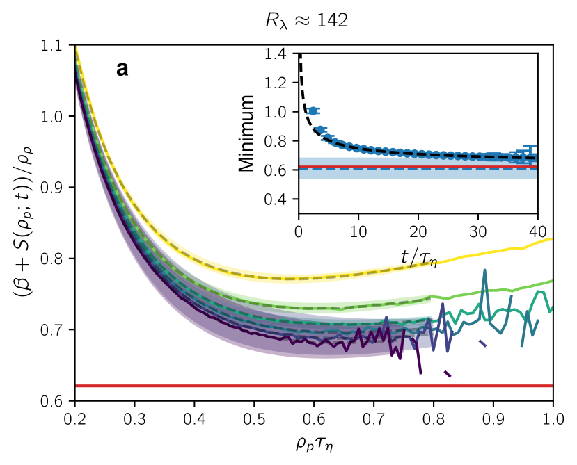
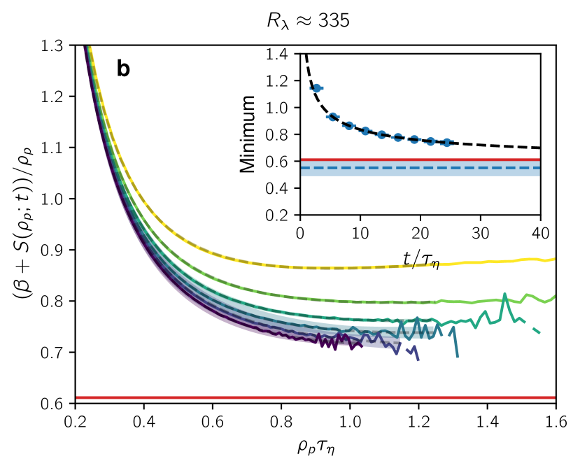
Refer to caption
Refer to caption
Supplementary Figure S5: Determination of the steepest-descent minimum for the supplementary simulations. a Low-Reynolds-number simulation with Cramér functions ranging from 7.26τη7.26subscript𝜏𝜂7.26\tau_{\eta} (yellow) up to 39.94τη39.94subscript𝜏𝜂39.94\tau_{\eta} (violet). Their fits are restricted to the range [λp(t),0.8/τη]subscript𝜆𝑝𝑡0.8subscript𝜏𝜂[\lambda_{p}(t),0.8/\tau_{\eta}], where λp(t)subscript𝜆𝑝𝑡\lambda_{p}(t) is the position of the minimum of S(ρp;t)𝑆subscript𝜌𝑝𝑡S(\rho_{p};t). Inset: Extrapolation of the minimum yields α=0.61±0.08𝛼plus-or-minus0.610.08\alpha=0.61\pm 0.08 (dashed blue line). b High-Reynolds-number simulation with Cramér functions at times ranging from 8.14τη8.14subscript𝜏𝜂8.14\tau_{\eta} (yellow) up to 35.26τη35.26subscript𝜏𝜂35.26\tau_{\eta} (violet). Their fits are restricted to the range [λp(t),1.25/τη]subscript𝜆𝑝𝑡1.25subscript𝜏𝜂[\lambda_{p}(t),1.25/\tau_{\eta}]. Inset: Extrapolation of the minimum yields α=0.55±0.07𝛼plus-or-minus0.550.07\alpha=0.55\pm 0.07 (dashed blue line). For comparison, in each plot the red line indicates the value of α𝛼\alpha estimated from the curvature PDF. For details on the procedure, see Methods.
Refer to caption
Refer to caption
Refer to caption
Supplementary Figure S6: Different fit choices for extrapolating the steepest-descent minimum. In order to compute the steepest-descent minimum (15), in principle we need a fully resolved Cramér function. In practice, however, we only have finite-time estimates of the Cramér function, which yield finite-time estimates of the minimum (our “data points” in the insets of Figs. 5 and S5). We use the simple decay function (24) to capture and extrapolate the evolution of these data points as a function of the time at which the finite-time Cramér function is computed. In order to obtain a satisfactory fit, it is helpful to leave out a transient regime of data points t<tmin𝑡subscript𝑡mint<t_{\mathrm{min}} such that only the asymptotic behavior is captured by the fit. Here we show the resulting values of α=A𝛼𝐴\alpha=A (top) and the decay exponent C𝐶C (middle) for different choices of tminsubscript𝑡mint_{\mathrm{min}} in all of the simulations (left to right). The time scale B𝐵B is not shown. We justify the choice of tminsubscript𝑡mint_{\mathrm{min}} by computing the weighted mean squared error (MSE, bottom) given by i=1N(δi/σi)2/(N3)superscriptsubscript𝑖1𝑁superscriptsubscript𝛿𝑖subscript𝜎𝑖2𝑁3\sum_{i=1}^{N}(\delta_{i}/\sigma_{i})^{2}/(N-3). Here, N𝑁N is the number of data points included, δisubscript𝛿𝑖\delta_{i} is the deviation of the fit from the i𝑖i-th data point, and σisubscript𝜎𝑖\sigma_{i} is the error of the i𝑖i-th data point, given by the maximum of the two-sided error computed from the error envelopes in Figs. 5 and S5. The quantity i=1N(δi/σi)2superscriptsubscript𝑖1𝑁superscriptsubscript𝛿𝑖subscript𝜎𝑖2\sum_{i=1}^{N}(\delta_{i}/\sigma_{i})^{2} is minimized by the fit, which we divide by the number of degrees of freedom N3𝑁3N-3 (number of data points minus number of fit parameters) for comparability. We choose tminsubscript𝑡mint_{\mathrm{min}} to be the start of the first plateau of the weighted MSE (red lines).

upplementary Note 2.   umerical analysis of generalized Lyapunov exponents

As a complementary approach to computing Cramér functions, we may also use generalized Lyapunov exponents (GLE) in order to determine the exponent α𝛼\alpha based on the implicit equation (47), in short: Lp(α)=β=L1(1)subscript𝐿𝑝𝛼𝛽subscript𝐿11L_{p}(\alpha)=\beta=L_{1}(1), where

L1(q)=limt1tlogexp(qρ1(t)t)subscript𝐿1𝑞subscript𝑡1𝑡𝑞subscript𝜌1𝑡𝑡\displaystyle L_{1}(q)=\lim_{t\to\infty}\frac{1}{t}\log\left\langle\exp(q\rho_{1}(t)t)\right\rangle (S1)

is the first standard GLE as opposed to

Lp(q)=limt1tlogexp(qρp(t)t),subscript𝐿𝑝𝑞subscript𝑡1𝑡𝑞subscript𝜌𝑝𝑡𝑡\displaystyle L_{p}(q)=\lim_{t\to\infty}\frac{1}{t}\log\left\langle\exp(q\rho_{p}(t)t)\right\rangle, (S2)

the curvature-peak GLE. For their numerical computation, we adopt the method from ref. [39]. We first compute the cumulant-generating function of ρ1(t)tsubscript𝜌1𝑡𝑡\rho_{1}(t)t, given by logexp(qρ1(t)t)𝑞subscript𝜌1𝑡𝑡\log\langle\exp(q\rho_{1}(t)t)\rangle, as a function of q𝑞q and t𝑡t. In order to estimate L1(q)subscript𝐿1𝑞L_{1}(q), we perform an affine fit of the cumulant-generating function in the range t[tmax/2,tmax]𝑡subscript𝑡max2subscript𝑡maxt\in[t_{\text{max}}/2,t_{\text{max}}], as exemplified in Fig. S7a for tmax=40τηsubscript𝑡max40subscript𝜏𝜂t_{\text{max}}=40\tau_{\eta}. The slope of each fit including its standard error becomes our estimate of L1(q)subscript𝐿1𝑞L_{1}(q). The same procedure is applied to Lp(q)subscript𝐿𝑝𝑞L_{p}(q).

For the main simulation, the results are shown in Fig. S7b. We can first read off the value of β𝛽\beta by evaluating L1(q)subscript𝐿1𝑞L_{1}(q) at q=1𝑞1q=1. Indeed, the different estimates for L1(1)subscript𝐿11L_{1}(1) appear to converge toward the value of β𝛽\beta previously estimated by other means. In order to estimate α𝛼\alpha, we need to read off the intersection of the β𝛽\beta-line with Lp(q)subscript𝐿𝑝𝑞L_{p}(q). For this curvature-peak GLE, we observe stronger fluctuations as a function of tmaxsubscript𝑡maxt_{\text{max}}. For small tmaxsubscript𝑡maxt_{\text{max}}, we expect the estimates of the cumulant-generating function to be accurate. However, if tmaxsubscript𝑡maxt_{\text{max}} is too small, we have not yet reached convergence of the t𝑡t\to\infty limit in the GLE. For larger tmaxsubscript𝑡maxt_{\text{max}}, we improve on the convergence of the GLE, but we also rely more heavily on extreme values of ρp(t)subscript𝜌𝑝𝑡\rho_{p}(t) (especially for large q𝑞q), which are limited by our sample size. Hence we expect the best estimate to be found at intermediate tmaxsubscript𝑡maxt_{\text{max}}. For the main simulation, we indeed find those intermediate curves to come closest to the value of α𝛼\alpha estimated from the curvature PDF. For the supplementary simulations (Fig. S8), the same argumentation holds and the estimates fluctuate as a function of tmaxsubscript𝑡maxt_{\text{max}} to a certain extent. If we simply read off α𝛼\alpha from the intersection of lines, the GLE method slightly overestimates α𝛼\alpha for all simulations, possibly due to both sampling and time-convergence limitations.
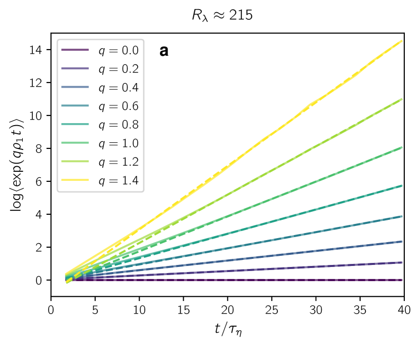
Refer to caption
Refer to caption
Supplementary Figure S7: Generalized Lyapunov exponents in the main simulation. a Plotting the cumulant-generating function of ρ1(t)tsubscript𝜌1𝑡𝑡\rho_{1}(t)t for fixed argument q𝑞q as a function of time (solid lines), the GLE L1(q)subscript𝐿1𝑞L_{1}(q) can be estimated as the asymptotic slope of the curve by an affine fit (dashed lines) on the interval t[tmax/2,tmax]𝑡subscript𝑡max2subscript𝑡maxt\in[t_{\text{max}}/2,t_{\text{max}}] where in this case tmax=40τηsubscript𝑡max40subscript𝜏𝜂t_{\text{max}}=40\tau_{\eta}. b Generalized Lyapunov exponents can be used to estimate β𝛽\beta and α𝛼\alpha. The first standard GLE L1(q)subscript𝐿1𝑞L_{1}(q) (solid lines) is shown for tmaxsubscript𝑡maxt_{\text{max}} ranging from 12.08τη12.08subscript𝜏𝜂12.08\tau_{\eta} (yellow) to 39.68τη39.68subscript𝜏𝜂39.68\tau_{\eta} (violet). The curvature-peak GLE Lp(q)subscript𝐿𝑝𝑞L_{p}(q) is shown for the same times (dashed lines). For comparison, we also show the line q=1𝑞1q=1 (solid, black), the value of β𝛽\beta estimated from curvature peak number (dotted, grey) and the value of α𝛼\alpha estimated from the curvature PDF (solid, red).
Refer to caption
Refer to caption
Supplementary Figure S8: Generalized Lyapunov exponents in the supplementary simulations, at low Reynolds number (a) and at high Reynolds number (b). As in the main simulation, the first standard GLE L1(1)subscript𝐿11L_{1}(1) converges toward the previously estimated value of β𝛽\beta, but the convergence is slower in the high-Reynolds-number simulation. Similarly, the value of α𝛼\alpha is slightly overestimated in both simulations. In a, tmaxsubscript𝑡maxt_{\text{max}} ranges from 12.10τη12.10subscript𝜏𝜂12.10\tau_{\eta} (yellow) to 39.94τη39.94subscript𝜏𝜂39.94\tau_{\eta} (violet). In b, tmaxsubscript𝑡maxt_{\text{max}} ranges from 16.27τη16.27subscript𝜏𝜂16.27\tau_{\eta} (yellow) to 35.26τη35.26subscript𝜏𝜂35.26\tau_{\eta} (violet). Note that the value of β𝛽\beta as a function of the Kolmogorov time scale τηsubscript𝜏𝜂\tau_{\eta} differs from the one in Fig. S4 because τηsubscript𝜏𝜂\tau_{\eta} is slightly different in the FTLE simulation.

upplementary Note 3.   aterial line bundles and flux cancellations

In the discussion, we explain how our results may help to shed light on the problem of flux cancellations in magnetohydrodynamics (MHD). Flux cancellations occur when magnetic field lines with opposite orientation are brought closely together by the flow and thus cancel each other in the integration of magnetic flux. In our simulations, we observe that the material lines are brought into such a configuration quite frequently (see Fig. S9). They even tend to form bundles of lines where about half of the lines has opposite orientation. Remarkably, these bundles appear to be strongly related to the sharp folds that lead to curvature peaks since the folds are typically observed in the middle or at the end of such bundles. Therefore, it may be worthwhile studying folds of the magnetic field in MHD (possibly detected by curvature peaks) and their relation to flux cancellations.
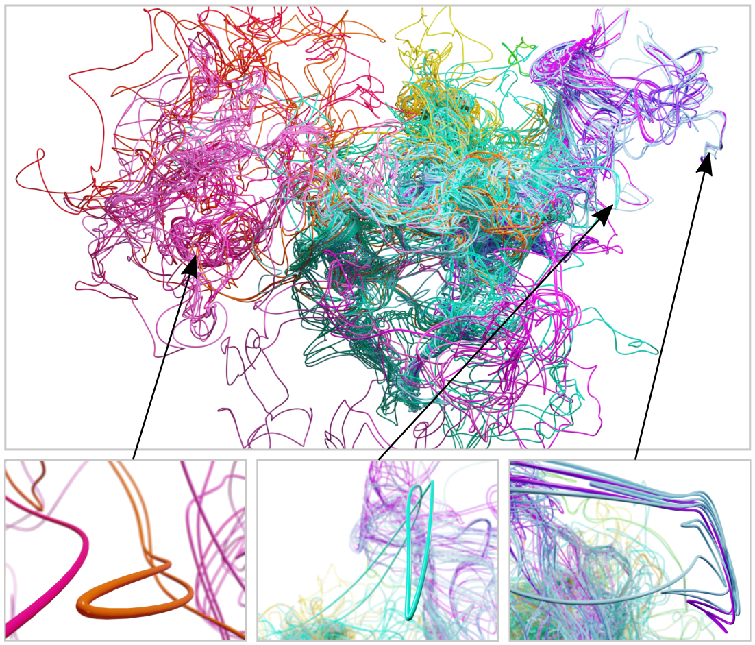
Refer to caption
Supplementary Figure S9: Loops form pairs and bundles of almost parallel material lines, which are closely associated with sharp folds. The loop snapshot is identical to Fig. 1 of the manuscript, taken at t=27τη𝑡27subscript𝜏𝜂t=27\tau_{\eta} in the main simulation at Rλ216subscript𝑅𝜆216R_{\lambda}\approx 216.

upplementary Note 4.   patial and temporal resolution of loop tracking

For tracking material loops in our simulations, we treated the sample points of the loops as Lagrangian tracers. Over time, new particles are inserted to sustain the necessary loop resolution. Since using higher-order time-stepping methods for the particles would require histories that are not available for newly inserted particles, we resorted to first-order Euler time stepping. In order to ensure the quality of our results, we tested the code with different temporal resolutions of flow and particle time stepping and different spatial resolution conditions of the loops. The results for simulations at Rλ146subscript𝑅𝜆146R_{\lambda}\approx 146 are shown in Fig. S10 where we compare curvature statistics for the different resolutions. We observe that neither an improved temporal resolution nor an improved spatial resolution of the loops leads to noticeable changes in the curvature distribution.
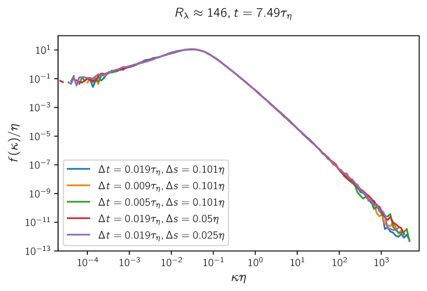
Refer to caption
Supplementary Figure S10: Curvature distributions for different temporal and spatial resolutions of the loops, taken from 1000 loops after 7.49τη7.49subscript𝜏𝜂7.49\tau_{\eta} in simulations at Rλ146subscript𝑅𝜆146R_{\lambda}\approx 146. ΔtΔ𝑡\Delta t is the time-step size of the simulation, including field and particle time stepping. ΔsΔ𝑠\Delta s denotes the maximum distance of sampling points of the loops enforced by the refinement. We adjusted the additional refinement condition based on curvature accordingly, effectively doubling the density of sample points uniformly along the loops when moving from Δs=0.1ηΔ𝑠0.1𝜂\Delta s=0.1\eta to Δs=0.05ηΔ𝑠0.05𝜂\Delta s=0.05\eta and further to Δs=0.025ηΔ𝑠0.025𝜂\Delta s=0.025\eta. Other parameters are identical with the low-Reynolds-number simulation shown in Supplementary Note 1, which uses Δt=0.018τηΔ𝑡0.018subscript𝜏𝜂\Delta t=0.018\tau_{\eta} and Δs=0.1ηΔ𝑠0.1𝜂\Delta s=0.1\eta. Note that the curved shape of the distribution can be attributed to the early time (t=7.49τη𝑡7.49subscript𝜏𝜂t=7.49\tau_{\eta}) in the loops’ evolution.

upplementary Note 5.   eometric evolution equations

Here, we derive the evolution equations (54)–(57). Implicitly, all quantities considered in these equations are evaluated along a material line element 𝐋=𝐋(ϕ,t)𝐋𝐋italic-ϕ𝑡\mathbf{L}=\mathbf{L}(\phi,t), whose evolution is given by the tracer equation (1). Therefore

tϕ𝐋(ϕ,t)subscript𝑡subscriptitalic-ϕ𝐋italic-ϕ𝑡\displaystyle\partial_{t}\partial_{\phi}\mathbf{L}(\phi,t) =((ϕ𝐋))𝐮(𝐋(ϕ,t),t)absentsubscriptitalic-ϕ𝐋𝐮𝐋italic-ϕ𝑡𝑡\displaystyle=((\partial_{\phi}\mathbf{L})\cdot\nabla)\mathbf{u}(\mathbf{L}(\phi,t),t) (S3)

which is (54). The evolution equation (55) for the tangent vector of the Frenet-Serret frame [19],

𝐭^(ϕ,t)=ϕ𝐋|ϕ𝐋|,^𝐭italic-ϕ𝑡subscriptitalic-ϕ𝐋subscriptitalic-ϕ𝐋\displaystyle\hat{\mathbf{t}}(\phi,t)=\frac{\partial_{\phi}\mathbf{L}}{\left|\partial_{\phi}\mathbf{L}\right|}, (S4)

can then be directly computed

t𝐭^(ϕ,t)subscript𝑡^𝐭italic-ϕ𝑡\displaystyle\partial_{t}\hat{\mathbf{t}}(\phi,t) =tϕ𝐋|ϕ𝐋|=1|ϕ𝐋|(ϕ𝐋)𝐮ϕ𝐋|ϕ𝐋|3ϕ𝐋(ϕ𝐋)𝐮=(𝐭^)𝐮(𝐭^(𝐭^)𝐮)𝐭^.absentsubscript𝑡subscriptitalic-ϕ𝐋subscriptitalic-ϕ𝐋1subscriptitalic-ϕ𝐋subscriptitalic-ϕ𝐋𝐮subscriptitalic-ϕ𝐋superscriptsubscriptitalic-ϕ𝐋3subscriptitalic-ϕ𝐋subscriptitalic-ϕ𝐋𝐮^𝐭𝐮^𝐭^𝐭𝐮^𝐭\displaystyle=\partial_{t}\frac{\partial_{\phi}\mathbf{L}}{\left|\partial_{\phi}\mathbf{L}\right|}=\frac{1}{\left|\partial_{\phi}\mathbf{L}\right|}(\partial_{\phi}\mathbf{L}\cdot\nabla)\mathbf{u}-\frac{\partial_{\phi}\mathbf{L}}{\left|\partial_{\phi}\mathbf{L}\right|^{3}}\partial_{\phi}\mathbf{L}\cdot(\partial_{\phi}\mathbf{L}\cdot\nabla)\mathbf{u}=(\hat{\mathbf{t}}\cdot\nabla)\mathbf{u}-(\hat{\mathbf{t}}\cdot(\hat{\mathbf{t}}\cdot\nabla)\mathbf{u})\hat{\mathbf{t}}. (S5)

The normal vector of the Frenet-Serret frame is defined as

𝐧^(ϕ,t)=s𝐭^|s𝐭^|,^𝐧italic-ϕ𝑡subscript𝑠^𝐭subscript𝑠^𝐭\displaystyle\hat{\mathbf{n}}(\phi,t)=\frac{\partial_{s}\hat{\mathbf{t}}}{|\partial_{s}\hat{\mathbf{t}}|}, (S6)

where s𝑠s denotes an arc-length parameterization of the line, i.e. |s𝐋|=1subscript𝑠𝐋1|\partial_{s}\mathbf{L}|=1. Since the transform from s𝑠s to ϕitalic-ϕ\phi is time-dependent, evaluating tsubscript𝑡\partial_{t} at constant ϕitalic-ϕ\phi and at constant s𝑠s are different operations. Here, we always want to take tsubscript𝑡\partial_{t} at constant ϕitalic-ϕ\phi (i.e. at the same tracer particle). Then, ssubscript𝑠\partial_{s} and tsubscript𝑡\partial_{t} do not commute. Having this in mind, we compute (summation over repeated indices implied)

tn^isubscript𝑡subscript^𝑛𝑖\displaystyle\partial_{t}\hat{n}_{i} =tst^i|s𝐭^|=(tst^i)|s𝐭^|(st^i)t|s𝐭^||s𝐭^|2=tst^i|s𝐭^|n^it|s𝐭^||s𝐭^|=tst^i|s𝐭^|n^in^j1|s𝐭^|tst^jabsentsubscript𝑡subscript𝑠subscript^𝑡𝑖subscript𝑠^𝐭subscript𝑡subscript𝑠subscript^𝑡𝑖subscript𝑠^𝐭subscript𝑠subscript^𝑡𝑖subscript𝑡subscript𝑠^𝐭superscriptsubscript𝑠^𝐭2subscript𝑡subscript𝑠subscript^𝑡𝑖subscript𝑠^𝐭subscript^𝑛𝑖subscript𝑡subscript𝑠^𝐭subscript𝑠^𝐭subscript𝑡subscript𝑠subscript^𝑡𝑖subscript𝑠^𝐭subscript^𝑛𝑖subscript^𝑛𝑗1subscript𝑠^𝐭subscript𝑡subscript𝑠subscript^𝑡𝑗\displaystyle=\partial_{t}\frac{\partial_{s}\hat{t}_{i}}{|\partial_{s}\hat{\mathbf{t}}|}=\frac{(\partial_{t}\partial_{s}\hat{t}_{i})|\partial_{s}\hat{\mathbf{t}}|-(\partial_{s}\hat{t}_{i})\partial_{t}|\partial_{s}\hat{\mathbf{t}}|}{|\partial_{s}\hat{\mathbf{t}}|^{2}}=\frac{\partial_{t}\partial_{s}\hat{t}_{i}}{|\partial_{s}\hat{\mathbf{t}}|}-\hat{n}_{i}\frac{\partial_{t}|\partial_{s}\hat{\mathbf{t}}|}{|\partial_{s}\hat{\mathbf{t}}|}=\frac{\partial_{t}\partial_{s}\hat{t}_{i}}{|\partial_{s}\hat{\mathbf{t}}|}-\hat{n}_{i}\hat{n}_{j}\frac{1}{|\partial_{s}\hat{\mathbf{t}}|}\partial_{t}\partial_{s}\hat{t}_{j}
=1|s𝐭^|(δijn^in^j)tst^j.absent1subscript𝑠^𝐭subscript𝛿𝑖𝑗subscript^𝑛𝑖subscript^𝑛𝑗subscript𝑡subscript𝑠subscript^𝑡𝑗\displaystyle=\frac{1}{|\partial_{s}\hat{\mathbf{t}}|}\left(\delta_{ij}-\hat{n}_{i}\hat{n}_{j}\right)\partial_{t}\partial_{s}\hat{t}_{j}. (S7)

In order to swap the t𝑡t- and s𝑠s-derivatives, we notice that s=dϕdsϕ=1|ϕ𝐋|ϕsubscript𝑠ditalic-ϕd𝑠subscriptitalic-ϕ1subscriptitalic-ϕ𝐋subscriptitalic-ϕ\partial_{s}=\mathinner{\tfrac{\operatorname{d\!}{}\phi}{\operatorname{d\!}{s}}}\partial_{\phi}=\frac{1}{|\partial_{\phi}\mathbf{L}|}\partial_{\phi}. Therefore

tst^jsubscript𝑡subscript𝑠subscript^𝑡𝑗\displaystyle\partial_{t}\partial_{s}\hat{t}_{j} =(t1|ϕ𝐋|)ϕt^j+stt^j=t^kt^l(kul)(st^j)+stt^j.absentsubscript𝑡1subscriptitalic-ϕ𝐋subscriptitalic-ϕsubscript^𝑡𝑗subscript𝑠subscript𝑡subscript^𝑡𝑗subscript^𝑡𝑘subscript^𝑡𝑙subscript𝑘subscript𝑢𝑙subscript𝑠subscript^𝑡𝑗subscript𝑠subscript𝑡subscript^𝑡𝑗\displaystyle=\left(\partial_{t}\frac{1}{|\partial_{\phi}\mathbf{L}|}\right)\partial_{\phi}\hat{t}_{j}+\partial_{s}\partial_{t}\hat{t}_{j}=-\hat{t}_{k}\hat{t}_{l}(\partial_{k}u_{l})(\partial_{s}\hat{t}_{j})+\partial_{s}\partial_{t}\hat{t}_{j}. (S8)

We then insert the evolution equation (S5) for the tangent vector 𝐭^^𝐭\hat{\mathbf{t}},

tst^jsubscript𝑡subscript𝑠subscript^𝑡𝑗\displaystyle\partial_{t}\partial_{s}\hat{t}_{j} =t^kt^l(kul)(st^j)+s((δjkt^jt^k)t^lluk)absentsubscript^𝑡𝑘subscript^𝑡𝑙subscript𝑘subscript𝑢𝑙subscript𝑠subscript^𝑡𝑗subscript𝑠subscript𝛿𝑗𝑘subscript^𝑡𝑗subscript^𝑡𝑘subscript^𝑡𝑙subscript𝑙subscript𝑢𝑘\displaystyle=-\hat{t}_{k}\hat{t}_{l}(\partial_{k}u_{l})(\partial_{s}\hat{t}_{j})+\partial_{s}\left((\delta_{jk}-\hat{t}_{j}\hat{t}_{k})\hat{t}_{l}\partial_{l}u_{k}\right)
=t^kt^l(kul)(st^j)((st^j)t^k+t^j(st^k))t^lluk+(δjkt^jt^k)((st^l)luk+t^lsluk)absentsubscript^𝑡𝑘subscript^𝑡𝑙subscript𝑘subscript𝑢𝑙subscript𝑠subscript^𝑡𝑗subscript𝑠subscript^𝑡𝑗subscript^𝑡𝑘subscript^𝑡𝑗subscript𝑠subscript^𝑡𝑘subscript^𝑡𝑙subscript𝑙subscript𝑢𝑘subscript𝛿𝑗𝑘subscript^𝑡𝑗subscript^𝑡𝑘subscript𝑠subscript^𝑡𝑙subscript𝑙subscript𝑢𝑘subscript^𝑡𝑙subscript𝑠subscript𝑙subscript𝑢𝑘\displaystyle=-\hat{t}_{k}\hat{t}_{l}(\partial_{k}u_{l})(\partial_{s}\hat{t}_{j})-\left((\partial_{s}\hat{t}_{j})\hat{t}_{k}+\hat{t}_{j}(\partial_{s}\hat{t}_{k})\right)\hat{t}_{l}\partial_{l}u_{k}+(\delta_{jk}-\hat{t}_{j}\hat{t}_{k})\left((\partial_{s}\hat{t}_{l})\partial_{l}u_{k}+\hat{t}_{l}\partial_{s}\partial_{l}u_{k}\right)
=|s𝐭^|[t^kt^ln^j(kul)(n^jt^k+t^jn^k)t^lluk+(δjkt^jt^k)(n^lluk+1|s𝐭^|t^lt^mlmuk)],absentsubscript𝑠^𝐭delimited-[]subscript^𝑡𝑘subscript^𝑡𝑙subscript^𝑛𝑗subscript𝑘subscript𝑢𝑙subscript^𝑛𝑗subscript^𝑡𝑘subscript^𝑡𝑗subscript^𝑛𝑘subscript^𝑡𝑙subscript𝑙subscript𝑢𝑘subscript𝛿𝑗𝑘subscript^𝑡𝑗subscript^𝑡𝑘subscript^𝑛𝑙subscript𝑙subscript𝑢𝑘1subscript𝑠^𝐭subscript^𝑡𝑙subscript^𝑡𝑚subscript𝑙subscript𝑚subscript𝑢𝑘\displaystyle=|\partial_{s}\hat{\mathbf{t}}|\Bigl{[}-\hat{t}_{k}\hat{t}_{l}\hat{n}_{j}(\partial_{k}u_{l})-(\hat{n}_{j}\hat{t}_{k}+\hat{t}_{j}\hat{n}_{k})\hat{t}_{l}\partial_{l}u_{k}+(\delta_{jk}-\hat{t}_{j}\hat{t}_{k})\Bigl{(}\hat{n}_{l}\partial_{l}u_{k}+\frac{1}{|\partial_{s}\hat{\mathbf{t}}|}\hat{t}_{l}\hat{t}_{m}\partial_{l}\partial_{m}u_{k}\Bigr{)}\Bigr{]}, (S9)

where in the last step we used (S6) and suk=t^mmuksubscript𝑠subscript𝑢𝑘subscript^𝑡𝑚subscript𝑚subscript𝑢𝑘\partial_{s}u_{k}=\hat{t}_{m}\partial_{m}u_{k}. Since |s𝐭^|=κ~subscript𝑠^𝐭~𝜅|\partial_{s}\hat{\mathbf{t}}|=\tilde{\kappa} and δij=t^it^j+n^in^j+b^ib^jsubscript𝛿𝑖𝑗subscript^𝑡𝑖subscript^𝑡𝑗subscript^𝑛𝑖subscript^𝑛𝑗subscript^𝑏𝑖subscript^𝑏𝑗\delta_{ij}=\hat{t}_{i}\hat{t}_{j}+\hat{n}_{i}\hat{n}_{j}+\hat{b}_{i}\hat{b}_{j}, we have

tn^isubscript𝑡subscript^𝑛𝑖\displaystyle\partial_{t}\hat{n}_{i} =(t^it^j+b^ib^j)[t^kt^ln^j(kul)(n^jt^k+t^jn^k)t^lluk+(n^jn^k+b^jb^k)(n^lluk+1κ~t^lt^mlmuk)]absentsubscript^𝑡𝑖subscript^𝑡𝑗subscript^𝑏𝑖subscript^𝑏𝑗delimited-[]subscript^𝑡𝑘subscript^𝑡𝑙subscript^𝑛𝑗subscript𝑘subscript𝑢𝑙subscript^𝑛𝑗subscript^𝑡𝑘subscript^𝑡𝑗subscript^𝑛𝑘subscript^𝑡𝑙subscript𝑙subscript𝑢𝑘subscript^𝑛𝑗subscript^𝑛𝑘subscript^𝑏𝑗subscript^𝑏𝑘subscript^𝑛𝑙subscript𝑙subscript𝑢𝑘1~𝜅subscript^𝑡𝑙subscript^𝑡𝑚subscript𝑙subscript𝑚subscript𝑢𝑘\displaystyle=(\hat{t}_{i}\hat{t}_{j}+\hat{b}_{i}\hat{b}_{j})\Bigl{[}-\hat{t}_{k}\hat{t}_{l}\hat{n}_{j}(\partial_{k}u_{l})-(\hat{n}_{j}\hat{t}_{k}+\hat{t}_{j}\hat{n}_{k})\hat{t}_{l}\partial_{l}u_{k}+(\hat{n}_{j}\hat{n}_{k}+\hat{b}_{j}\hat{b}_{k})\Bigl{(}\hat{n}_{l}\partial_{l}u_{k}+\frac{1}{\tilde{\kappa}}\hat{t}_{l}\hat{t}_{m}\partial_{l}\partial_{m}u_{k}\Bigr{)}\Bigr{]}
=t^in^kt^lluk+b^ib^kn^lluk+1κ~b^ib^kt^lt^mlmuk,absentsubscript^𝑡𝑖subscript^𝑛𝑘subscript^𝑡𝑙subscript𝑙subscript𝑢𝑘subscript^𝑏𝑖subscript^𝑏𝑘subscript^𝑛𝑙subscript𝑙subscript𝑢𝑘1~𝜅subscript^𝑏𝑖subscript^𝑏𝑘subscript^𝑡𝑙subscript^𝑡𝑚subscript𝑙subscript𝑚subscript𝑢𝑘\displaystyle=-\hat{t}_{i}\hat{n}_{k}\hat{t}_{l}\partial_{l}u_{k}+\hat{b}_{i}\hat{b}_{k}\hat{n}_{l}\partial_{l}u_{k}+\frac{1}{\tilde{\kappa}}\hat{b}_{i}\hat{b}_{k}\hat{t}_{l}\hat{t}_{m}\partial_{l}\partial_{m}u_{k}, (S10)

where we also used orthonormality of the Frenet-Serret frame. This is (Fokker-Planck equation of curvature in the Kraichnan model).

Finally, in order to derive the curvature evolution equation, we use a simple definition as a function of the tangent vector with arc-length parameterization,

κ~(ϕ,t)=|s𝐭^|,~𝜅italic-ϕ𝑡subscript𝑠^𝐭\tilde{\kappa}(\phi,t)=|\partial_{s}\hat{\mathbf{t}}|, (S11)

which is equivalent to definition (2). Using the previous results, we obtain

tκ~subscript𝑡~𝜅\displaystyle\partial_{t}\tilde{\kappa} =t|s𝐭^|=n^jtst^j=n^jκ~[t^kt^ln^j(kul)(n^jt^k+t^jn^k)t^lluk+(n^jn^k+b^jb^k)(n^lluk+1|s𝐭^|t^lt^mlmuk)]absentsubscript𝑡subscript𝑠^𝐭subscript^𝑛𝑗subscript𝑡subscript𝑠subscript^𝑡𝑗subscript^𝑛𝑗~𝜅delimited-[]subscript^𝑡𝑘subscript^𝑡𝑙subscript^𝑛𝑗subscript𝑘subscript𝑢𝑙subscript^𝑛𝑗subscript^𝑡𝑘subscript^𝑡𝑗subscript^𝑛𝑘subscript^𝑡𝑙subscript𝑙subscript𝑢𝑘subscript^𝑛𝑗subscript^𝑛𝑘subscript^𝑏𝑗subscript^𝑏𝑘subscript^𝑛𝑙subscript𝑙subscript𝑢𝑘1subscript𝑠^𝐭subscript^𝑡𝑙subscript^𝑡𝑚subscript𝑙subscript𝑚subscript𝑢𝑘\displaystyle=\partial_{t}|\partial_{s}\hat{\mathbf{t}}|=\hat{n}_{j}\partial_{t}\partial_{s}\hat{t}_{j}=\hat{n}_{j}\tilde{\kappa}\Bigl{[}-\hat{t}_{k}\hat{t}_{l}\hat{n}_{j}(\partial_{k}u_{l})-(\hat{n}_{j}\hat{t}_{k}+\hat{t}_{j}\hat{n}_{k})\hat{t}_{l}\partial_{l}u_{k}+(\hat{n}_{j}\hat{n}_{k}+\hat{b}_{j}\hat{b}_{k})\Bigl{(}\hat{n}_{l}\partial_{l}u_{k}+\frac{1}{|\partial_{s}\hat{\mathbf{t}}|}\hat{t}_{l}\hat{t}_{m}\partial_{l}\partial_{m}u_{k}\Bigr{)}\Bigr{]}
=κ~(2t^kt^l+n^kn^l)kul+n^kt^lt^mlmuk.absent~𝜅2subscript^𝑡𝑘subscript^𝑡𝑙subscript^𝑛𝑘subscript^𝑛𝑙subscript𝑘subscript𝑢𝑙subscript^𝑛𝑘subscript^𝑡𝑙subscript^𝑡𝑚subscript𝑙subscript𝑚subscript𝑢𝑘\displaystyle=\tilde{\kappa}\Bigl{(}-2\hat{t}_{k}\hat{t}_{l}+\hat{n}_{k}\hat{n}_{l}\Bigr{)}\partial_{k}u_{l}+\hat{n}_{k}\hat{t}_{l}\hat{t}_{m}\partial_{l}\partial_{m}u_{k}. (S12)

This is (57), which can also be found in ref. [22].

upplementary Note 6.   okker-Planck equation in the Kraichnan model

In Methods, we laid out the terms that need to be calculated in order to arrive at the Fokker-Planck equation in the Kraichnan model. In order to proceed, we combine (53) with the evolution equations derived in the previous section and get

tf(κ;t)subscript𝑡𝑓𝜅𝑡\displaystyle\partial_{t}f(\kappa;t) =δ(κκ~)t|ϕ𝐋||ϕ𝐋|f(κ;t)t|ϕ𝐋||ϕ𝐋|1|ϕ𝐋|κδ(κκ~)|ϕ𝐋|tκ~absentdelimited-⟨⟩𝛿𝜅~𝜅subscript𝑡subscriptitalic-ϕ𝐋delimited-⟨⟩subscriptitalic-ϕ𝐋𝑓𝜅𝑡subscript𝑡delimited-⟨⟩subscriptitalic-ϕ𝐋delimited-⟨⟩subscriptitalic-ϕ𝐋1delimited-⟨⟩subscriptitalic-ϕ𝐋subscript𝜅quantum-operator-product𝛿𝜅~𝜅subscriptitalic-ϕ𝐋subscript𝑡~𝜅\displaystyle=\frac{\left\langle\delta(\kappa-\tilde{\kappa})\partial_{t}|\partial_{\phi}\mathbf{L}|\right\rangle}{\left\langle|\partial_{\phi}\mathbf{L}|\right\rangle}-f(\kappa;t)\frac{\partial_{t}\left\langle|\partial_{\phi}\mathbf{L}|\right\rangle}{\left\langle|\partial_{\phi}\mathbf{L}|\right\rangle}-\frac{1}{\left\langle|\partial_{\phi}\mathbf{L}|\right\rangle}\partial_{\kappa}\left\langle\delta(\kappa-\tilde{\kappa})|\partial_{\phi}\mathbf{L}|\partial_{t}\tilde{\kappa}\right\rangle (S13)
=1|ϕ𝐋|(|ϕ𝐋|δ(κκ~)t^it^jjuif(κ;t)|ϕ𝐋|t^it^jjui\displaystyle=\frac{1}{\left\langle|\partial_{\phi}\mathbf{L}|\right\rangle}\Biggl{(}\left\langle|\partial_{\phi}\mathbf{L}|\delta(\kappa-\tilde{\kappa})\hat{t}_{i}\hat{t}_{j}\partial_{j}u_{i}\right\rangle-f(\kappa;t)\left\langle|\partial_{\phi}\mathbf{L}|\hat{t}_{i}\hat{t}_{j}\partial_{j}u_{i}\right\rangle (S14)
κ(2κ|ϕ𝐋|δ(κκ~)t^it^jjui+κ|ϕ𝐋|δ(κκ~)n^in^jjui+|ϕ𝐋|δ(κκ~)n^it^jt^kjkui)).\displaystyle\quad-\partial_{\kappa}\Bigl{(}-2\kappa\Bigl{\langle}|\partial_{\phi}\mathbf{L}|\delta(\kappa-\tilde{\kappa})\hat{t}_{i}\hat{t}_{j}\partial_{j}u_{i}\Bigr{\rangle}+\kappa\Bigl{\langle}|\partial_{\phi}\mathbf{L}|\delta(\kappa-\tilde{\kappa})\hat{n}_{i}\hat{n}_{j}\partial_{j}u_{i}\Bigr{\rangle}+\Bigl{\langle}|\partial_{\phi}\mathbf{L}|\delta(\kappa-\tilde{\kappa})\hat{n}_{i}\hat{t}_{j}\hat{t}_{k}\partial_{j}\partial_{k}u_{i}\Bigr{\rangle}\Bigr{)}\Biggr{)}.

We want to evaluate these averages using the Gaussian integration by parts formula [58, 59, 60] combined with the correlation tensor (51). This works analogously for all of them. So let us focus on one of the averages. By introducing delta functions, we can consider the velocity field at the Eulerian coordinate 𝐱𝐱\mathbf{x} and take the derivative out of the average (the other quantities are still evaluated at 𝐋(ϕ,t)𝐋italic-ϕ𝑡\mathbf{L}(\phi,t)),

|ϕ𝐋|δ(κκ~)n^in^jjuidelimited-⟨⟩subscriptitalic-ϕ𝐋𝛿𝜅~𝜅subscript^𝑛𝑖subscript^𝑛𝑗subscript𝑗subscript𝑢𝑖\displaystyle\langle|\partial_{\phi}\mathbf{L}|\delta(\kappa-\tilde{\kappa})\hat{n}_{i}\hat{n}_{j}\partial_{j}u_{i}\rangle =d3𝐱d3𝐲δ(𝐱𝐲)xj|ϕ𝐋|δ(𝐲𝐋(ϕ,t))δ(κκ~)n^in^jui(𝐱,t).absentsuperscriptd3𝐱superscriptd3𝐲𝛿𝐱𝐲subscript𝑥𝑗delimited-⟨⟩subscriptitalic-ϕ𝐋𝛿𝐲𝐋italic-ϕ𝑡𝛿𝜅~𝜅subscript^𝑛𝑖subscript^𝑛𝑗subscript𝑢𝑖𝐱𝑡\displaystyle=\int\mathrm{d^{3}}\mathbf{x}\int\mathrm{d^{3}}\mathbf{y}~{}\delta(\mathbf{x}-\mathbf{y})\mathinner{\dfrac{\partial{}}{\partial{x_{j}}}}\left\langle|\partial_{\phi}\mathbf{L}|\delta(\mathbf{y}-\mathbf{L}(\phi,t))\delta(\kappa-\tilde{\kappa})\hat{n}_{i}\hat{n}_{j}u_{i}(\mathbf{x},t)\right\rangle. (S15)

Then Gaussian integration by parts yields

|ϕ𝐋|δ(κκ~)n^in^jjuidelimited-⟨⟩subscriptitalic-ϕ𝐋𝛿𝜅~𝜅subscript^𝑛𝑖subscript^𝑛𝑗subscript𝑗subscript𝑢𝑖\displaystyle\langle|\partial_{\phi}\mathbf{L}|\delta(\kappa-\tilde{\kappa})\hat{n}_{i}\hat{n}_{j}\partial_{j}u_{i}\rangle =d3𝐱d3𝐲δ(𝐱𝐲)xjd3𝐳Rik(𝐱𝐳)δ[|ϕ𝐋|δ(𝐲𝐋(ϕ,t))δ(κκ~)n^in^j]δuk(𝐳,t)absentsuperscriptd3𝐱superscriptd3𝐲𝛿𝐱𝐲subscript𝑥𝑗superscriptd3𝐳subscript𝑅𝑖𝑘𝐱𝐳delimited-⟨⟩𝛿delimited-[]subscriptitalic-ϕ𝐋𝛿𝐲𝐋italic-ϕ𝑡𝛿𝜅~𝜅subscript^𝑛𝑖subscript^𝑛𝑗𝛿subscript𝑢𝑘𝐳𝑡\displaystyle=\int\mathrm{d^{3}}\mathbf{x}\int\mathrm{d^{3}}\mathbf{y}~{}\delta(\mathbf{x}-\mathbf{y})\mathinner{\dfrac{\partial{}}{\partial{x_{j}}}}\int\mathrm{d^{3}}\mathbf{z}~{}R_{ik}(\mathbf{x}-\mathbf{z})\left\langle\frac{\delta\left[|\partial_{\phi}\mathbf{L}|\delta(\mathbf{y}-\mathbf{L}(\phi,t))\delta(\kappa-\tilde{\kappa})\hat{n}_{i}\hat{n}_{j}\right]}{\delta u_{k}(\mathbf{z},t)}\right\rangle
=d3𝐱d3𝐳(jRik(𝐱𝐳))δ[|ϕ𝐋|δ(𝐱𝐋(ϕ,t))δ(κκ~)n^in^j]δuk(𝐳,t).absentsuperscriptd3𝐱superscriptd3𝐳subscript𝑗subscript𝑅𝑖𝑘𝐱𝐳delimited-⟨⟩𝛿delimited-[]subscriptitalic-ϕ𝐋𝛿𝐱𝐋italic-ϕ𝑡𝛿𝜅~𝜅subscript^𝑛𝑖subscript^𝑛𝑗𝛿subscript𝑢𝑘𝐳𝑡\displaystyle=\int\mathrm{d^{3}}\mathbf{x}\int\mathrm{d^{3}}\mathbf{z}~{}\left(\partial_{j}R_{ik}(\mathbf{x}-\mathbf{z})\right)\left\langle\frac{\delta\left[|\partial_{\phi}\mathbf{L}|\delta(\mathbf{x}-\mathbf{L}(\phi,t))\delta(\kappa-\tilde{\kappa})\hat{n}_{i}\hat{n}_{j}\right]}{\delta u_{k}(\mathbf{z},t)}\right\rangle. (S16)

The product rule for the functional derivative yields five different terms, which can all be treated in the same way. Let us again focus on a single one of them, namely

M𝑀\displaystyle M =d3𝐱d3𝐳(jRik(𝐱𝐳))|ϕ𝐋|δ(𝐱𝐋(ϕ,t))n^in^jδ[δ(κκ~)]δuk(𝐳,t)absentsuperscriptd3𝐱superscriptd3𝐳subscript𝑗subscript𝑅𝑖𝑘𝐱𝐳delimited-⟨⟩subscriptitalic-ϕ𝐋𝛿𝐱𝐋italic-ϕ𝑡subscript^𝑛𝑖subscript^𝑛𝑗𝛿delimited-[]𝛿𝜅~𝜅𝛿subscript𝑢𝑘𝐳𝑡\displaystyle=\int\mathrm{d^{3}}\mathbf{x}\int\mathrm{d^{3}}\mathbf{z}~{}\left(\partial_{j}R_{ik}(\mathbf{x}-\mathbf{z})\right)\left\langle|\partial_{\phi}\mathbf{L}|\delta(\mathbf{x}-\mathbf{L}(\phi,t))\hat{n}_{i}\hat{n}_{j}\frac{\delta\left[\delta(\kappa-\tilde{\kappa})\right]}{\delta u_{k}(\mathbf{z},t)}\right\rangle
=d3𝐳(jRik(𝐋(ϕ,t)𝐳))|ϕ𝐋|n^in^jδ(κ~κ)δκ~δuk(𝐳,t).absentsuperscriptd3𝐳quantum-operator-productsubscript𝑗subscript𝑅𝑖𝑘𝐋italic-ϕ𝑡𝐳subscriptitalic-ϕ𝐋subscript^𝑛𝑖subscript^𝑛𝑗superscript𝛿~𝜅𝜅𝛿~𝜅𝛿subscript𝑢𝑘𝐳𝑡\displaystyle=\int\mathrm{d^{3}}\mathbf{z}~{}\left\langle\left(\partial_{j}R_{ik}(\mathbf{L}(\phi,t)-\mathbf{z})\right)|\partial_{\phi}\mathbf{L}|\hat{n}_{i}\hat{n}_{j}\delta^{\prime}(\tilde{\kappa}-\kappa)\frac{\delta\tilde{\kappa}}{\delta u_{k}(\mathbf{z},t)}\right\rangle. (S17)

In order to determine the response function δκ~δuk(𝐳,t)𝛿~𝜅𝛿subscript𝑢𝑘𝐳𝑡\frac{\delta\tilde{\kappa}}{\delta u_{k}(\mathbf{z},t)}, we formally integrate the curvature evolution equation (S12),

κ~(ϕ,t)~𝜅italic-ϕ𝑡\displaystyle\tilde{\kappa}(\phi,t) =κ~(ϕ,0)+0tdt(κ~n^mn^nnum2κ~t^mt^nnum+n^mt^nt^onoum)|(𝐋(ϕ,t),t).\displaystyle=\tilde{\kappa}(\phi,0)+\int_{0}^{t}\operatorname{d\!}t^{\prime}~{}\mathinner{\left(\tilde{\kappa}\hat{n}_{m}\hat{n}_{n}\partial_{n}u_{m}-2\tilde{\kappa}\hat{t}_{m}\hat{t}_{n}\partial_{n}u_{m}+\hat{n}_{m}\hat{t}_{n}\hat{t}_{o}\partial_{n}\partial_{o}u_{m}\right)\Biggr{\rvert}}_{(\mathbf{L}(\phi,t^{\prime}),t^{\prime})}. (S18)

By causality, the initial condition will not depend on uk(𝐳,t)subscript𝑢𝑘𝐳𝑡u_{k}(\mathbf{z},t) for t>0𝑡0t>0. The integrand will not depend on uk(𝐳,t)subscript𝑢𝑘𝐳𝑡u_{k}(\mathbf{z},t) for all t<tsuperscript𝑡𝑡t^{\prime}<t either, and the only contribution to the functional derivative can come from the time t=tsuperscript𝑡𝑡t^{\prime}=t. Since κ~~𝜅\tilde{\kappa}, 𝐧^^𝐧\hat{\mathbf{n}}, and 𝐭^^𝐭\hat{\mathbf{t}} are integrated quantities of the delta-correlated field 𝐮𝐮\mathbf{u}, we expect them to be continuous in time, just like a Wiener process is continuous while its differential is not. Hence their response functions will only be finite, thus not contribute to the integral. Using that

δum(𝐋(ϕ,t),t)δuk(𝐳,t)𝛿subscript𝑢𝑚𝐋italic-ϕsuperscript𝑡superscript𝑡𝛿subscript𝑢𝑘𝐳𝑡\displaystyle\frac{\delta u_{m}(\mathbf{L}(\phi,t^{\prime}),t^{\prime})}{\delta u_{k}(\mathbf{z},t)} =δ(𝐋(ϕ,t)𝐳)δ(tt)δmk,absent𝛿𝐋italic-ϕsuperscript𝑡𝐳𝛿𝑡superscript𝑡subscript𝛿𝑚𝑘\displaystyle=\delta(\mathbf{L}(\phi,t^{\prime})-\mathbf{z})\delta(t-t^{\prime})\delta_{mk}, (S19)

the response function becomes

δκ~(ϕ,t)δuk(𝐳,t)𝛿~𝜅italic-ϕ𝑡𝛿subscript𝑢𝑘𝐳𝑡\displaystyle\frac{\delta\tilde{\kappa}(\phi,t)}{\delta u_{k}(\mathbf{z},t)} =12(κ~n^kn^nnδ(𝐋(ϕ,t)𝐳)2κ~t^kt^nnδ(𝐋(ϕ,t)𝐳)+n^kt^nt^onoδ(𝐋(ϕ,t)𝐳)),absent12~𝜅subscript^𝑛𝑘subscript^𝑛𝑛subscript𝑛𝛿𝐋italic-ϕ𝑡𝐳2~𝜅subscript^𝑡𝑘subscript^𝑡𝑛subscript𝑛𝛿𝐋italic-ϕ𝑡𝐳subscript^𝑛𝑘subscript^𝑡𝑛subscript^𝑡𝑜subscript𝑛subscript𝑜𝛿𝐋italic-ϕ𝑡𝐳\displaystyle=\frac{1}{2}\Bigl{(}\tilde{\kappa}\hat{n}_{k}\hat{n}_{n}\partial_{n}\delta(\mathbf{L}(\phi,t)-\mathbf{z})-2\tilde{\kappa}\hat{t}_{k}\hat{t}_{n}\partial_{n}\delta(\mathbf{L}(\phi,t)-\mathbf{z})+\hat{n}_{k}\hat{t}_{n}\hat{t}_{o}\partial_{n}\partial_{o}\delta(\mathbf{L}(\phi,t)-\mathbf{z})\Bigr{)},

where the factor 1212\frac{1}{2} comes from the fact that only half of the delta function δ(tt)𝛿𝑡superscript𝑡\delta(t-t^{\prime}) is contained in the integration range [0,t]0𝑡[0,t]. Using integration by parts and the sifting property of the delta function, our term M𝑀M can thus be simplified to

M𝑀\displaystyle M =12κ((jnRik(𝟎))κ|ϕ𝐋|n^in^jδ(κκ~)(n^kn^n2t^kt^n)(jnoRik(𝟎))|ϕ𝐋|n^in^jδ(κκ~)n^kt^nt^o).absent12subscript𝜅subscript𝑗subscript𝑛subscript𝑅𝑖𝑘0𝜅delimited-⟨⟩subscriptitalic-ϕ𝐋subscript^𝑛𝑖subscript^𝑛𝑗𝛿𝜅~𝜅subscript^𝑛𝑘subscript^𝑛𝑛2subscript^𝑡𝑘subscript^𝑡𝑛subscript𝑗subscript𝑛subscript𝑜subscript𝑅𝑖𝑘0delimited-⟨⟩subscriptitalic-ϕ𝐋subscript^𝑛𝑖subscript^𝑛𝑗𝛿𝜅~𝜅subscript^𝑛𝑘subscript^𝑡𝑛subscript^𝑡𝑜\displaystyle=\frac{1}{2}\partial_{\kappa}\Biggl{(}\left(\partial_{j}\partial_{n}R_{ik}(\mathbf{0})\right)\kappa\left\langle|\partial_{\phi}\mathbf{L}|\hat{n}_{i}\hat{n}_{j}\delta(\kappa-\tilde{\kappa})(\hat{n}_{k}\hat{n}_{n}-2\hat{t}_{k}\hat{t}_{n})\right\rangle-\left(\partial_{j}\partial_{n}\partial_{o}R_{ik}(\mathbf{0})\right)\left\langle|\partial_{\phi}\mathbf{L}|\hat{n}_{i}\hat{n}_{j}\delta(\kappa-\tilde{\kappa})\hat{n}_{k}\hat{t}_{n}\hat{t}_{o}\right\rangle\Biggr{)}.

Although the spatial correlation tensor Rik(𝐫)subscript𝑅𝑖𝑘𝐫R_{ik}(\mathbf{r}) can be freely chosen, we can restrict its functional form by assuming isotropy and incompressibility of the Kraichnan field. By isotropy the correlation tensor must be even, hence odd derivatives vanish at zero, e.g. jnoRik(𝟎)=0subscript𝑗subscript𝑛subscript𝑜subscript𝑅𝑖𝑘00\partial_{j}\partial_{n}\partial_{o}R_{ik}(\mathbf{0})=0. For the second derivatives, we know that they must have the general form of an isotropic rank-4 tensor [62],

Qjnik=jnRik(𝟎)=Aδikδjn+Bδijδkn+Cδinδjk.superscriptsubscript𝑄𝑗𝑛𝑖𝑘subscript𝑗subscript𝑛subscript𝑅𝑖𝑘0𝐴subscript𝛿𝑖𝑘subscript𝛿𝑗𝑛𝐵subscript𝛿𝑖𝑗subscript𝛿𝑘𝑛𝐶subscript𝛿𝑖𝑛subscript𝛿𝑗𝑘\displaystyle Q_{jn}^{ik}=-\partial_{j}\partial_{n}R_{ik}(\mathbf{0})=A\delta_{ik}\delta_{jn}+B\delta_{ij}\delta_{kn}+C\delta_{in}\delta_{jk}. (S20)

By definition, this tensor must be symmetric under exchange of j𝑗j and n𝑛n, which implies B=C𝐵𝐶B=C. Finally, incompressibility implies δijQjnik=0subscript𝛿𝑖𝑗superscriptsubscript𝑄𝑗𝑛𝑖𝑘0\delta_{ij}Q_{jn}^{ik}=0 so that

A𝐴\displaystyle A =4B,absent4𝐵\displaystyle=-4B, (S21)

leading to the general form [61]

Qjnik=Q(4δikδjnδijδknδinδjk).superscriptsubscript𝑄𝑗𝑛𝑖𝑘𝑄4subscript𝛿𝑖𝑘subscript𝛿𝑗𝑛subscript𝛿𝑖𝑗subscript𝛿𝑘𝑛subscript𝛿𝑖𝑛subscript𝛿𝑗𝑘\displaystyle Q_{jn}^{ik}=Q(4\delta_{ik}\delta_{jn}-\delta_{ij}\delta_{kn}-\delta_{in}\delta_{jk}). (S22)

Analogous arguments can be used to deduce the general form (59) of the fourth-order derivatives of the correlation tensor. Using this expression, our term M𝑀M can be evaluated,

M𝑀\displaystyle M =12Qκ((4δikδjnδijδknδinδjk)κ|ϕ𝐋|n^in^jδ(κκ~)(n^kn^n2t^kt^n))absent12𝑄subscript𝜅4subscript𝛿𝑖𝑘subscript𝛿𝑗𝑛subscript𝛿𝑖𝑗subscript𝛿𝑘𝑛subscript𝛿𝑖𝑛subscript𝛿𝑗𝑘𝜅delimited-⟨⟩subscriptitalic-ϕ𝐋subscript^𝑛𝑖subscript^𝑛𝑗𝛿𝜅~𝜅subscript^𝑛𝑘subscript^𝑛𝑛2subscript^𝑡𝑘subscript^𝑡𝑛\displaystyle=-\frac{1}{2}Q\partial_{\kappa}\left((4\delta_{ik}\delta_{jn}-\delta_{ij}\delta_{kn}-\delta_{in}\delta_{jk})\kappa\left\langle|\partial_{\phi}\mathbf{L}|\hat{n}_{i}\hat{n}_{j}\delta(\kappa-\tilde{\kappa})(\hat{n}_{k}\hat{n}_{n}-2\hat{t}_{k}\hat{t}_{n})\right\rangle\right)
=2Qκ(κf(κ;t))|ϕ𝐋|,absent2𝑄subscript𝜅𝜅𝑓𝜅𝑡delimited-⟨⟩subscriptitalic-ϕ𝐋\displaystyle=-2Q\partial_{\kappa}\left(\kappa f(\kappa;t)\right)\left\langle|\partial_{\phi}\mathbf{L}|\right\rangle, (S23)

by orthonormality of the Frenet-Serret frame.

In the following, we list all the terms that need to be computed along with the results of their evaluation. By Gaussian integration by parts and the product rule for functional derivatives, the averages of (S14) split into

|ϕ𝐋|δ(κκ~)t^it^jjuidelimited-⟨⟩subscriptitalic-ϕ𝐋𝛿𝜅~𝜅subscript^𝑡𝑖subscript^𝑡𝑗subscript𝑗subscript𝑢𝑖\displaystyle\langle|\partial_{\phi}\mathbf{L}|\delta(\kappa-\tilde{\kappa})\hat{t}_{i}\hat{t}_{j}\partial_{j}u_{i}\rangle =d3𝐳(jRik(𝐋(ϕ,t)𝐳))δ(κκ~)t^it^jδ|ϕ𝐋|δuk(𝐳,t)absentsuperscriptd3𝐳delimited-⟨⟩subscript𝑗subscript𝑅𝑖𝑘𝐋italic-ϕ𝑡𝐳𝛿𝜅~𝜅subscript^𝑡𝑖subscript^𝑡𝑗𝛿subscriptitalic-ϕ𝐋𝛿subscript𝑢𝑘𝐳𝑡\displaystyle=\int\mathrm{d^{3}}\mathbf{z}~{}\left\langle\left(\partial_{j}R_{ik}(\mathbf{L}(\phi,t)-\mathbf{z})\right)\delta(\kappa-\tilde{\kappa})\hat{t}_{i}\hat{t}_{j}\frac{\delta|\partial_{\phi}\mathbf{L}|}{\delta u_{k}(\mathbf{z},t)}\right\rangle (S24)
+d3𝐳(jRik(𝐋(ϕ,t)𝐳))|ϕ𝐋|t^it^jδ[δ(κκ~)]δuk(𝐳,t)superscriptd3𝐳quantum-operator-productsubscript𝑗subscript𝑅𝑖𝑘𝐋italic-ϕ𝑡𝐳subscriptitalic-ϕ𝐋subscript^𝑡𝑖subscript^𝑡𝑗𝛿delimited-[]𝛿𝜅~𝜅𝛿subscript𝑢𝑘𝐳𝑡\displaystyle\qquad+\int\mathrm{d^{3}}\mathbf{z}~{}\left\langle\left(\partial_{j}R_{ik}(\mathbf{L}(\phi,t)-\mathbf{z})\right)|\partial_{\phi}\mathbf{L}|\hat{t}_{i}\hat{t}_{j}\frac{\delta\left[\delta(\kappa-\tilde{\kappa})\right]}{\delta u_{k}(\mathbf{z},t)}\right\rangle (S25)
+d3𝐳(jRik(𝐋(ϕ,t)𝐳))|ϕ𝐋|δ(κκ~)t^jδt^iδuk(𝐳,t)superscriptd3𝐳quantum-operator-productsubscript𝑗subscript𝑅𝑖𝑘𝐋italic-ϕ𝑡𝐳subscriptitalic-ϕ𝐋𝛿𝜅~𝜅subscript^𝑡𝑗𝛿subscript^𝑡𝑖𝛿subscript𝑢𝑘𝐳𝑡\displaystyle\qquad+\int\mathrm{d^{3}}\mathbf{z}~{}\left\langle\left(\partial_{j}R_{ik}(\mathbf{L}(\phi,t)-\mathbf{z})\right)|\partial_{\phi}\mathbf{L}|\delta(\kappa-\tilde{\kappa})\hat{t}_{j}\frac{\delta\hat{t}_{i}}{\delta u_{k}(\mathbf{z},t)}\right\rangle (S26)
+d3𝐳(jRik(𝐋(ϕ,t)𝐳))|ϕ𝐋|δ(κκ~)t^iδt^jδuk(𝐳,t)superscriptd3𝐳quantum-operator-productsubscript𝑗subscript𝑅𝑖𝑘𝐋italic-ϕ𝑡𝐳subscriptitalic-ϕ𝐋𝛿𝜅~𝜅subscript^𝑡𝑖𝛿subscript^𝑡𝑗𝛿subscript𝑢𝑘𝐳𝑡\displaystyle\qquad+\int\mathrm{d^{3}}\mathbf{z}~{}\left\langle\left(\partial_{j}R_{ik}(\mathbf{L}(\phi,t)-\mathbf{z})\right)|\partial_{\phi}\mathbf{L}|\delta(\kappa-\tilde{\kappa})\hat{t}_{i}\frac{\delta\hat{t}_{j}}{\delta u_{k}(\mathbf{z},t)}\right\rangle (S27)
+d3𝐱d3𝐳(jRik(𝐱𝐳))|ϕ𝐋|δ(κκ~)t^it^jδ[δ(𝐱𝐋(ϕ,t))]δuk(𝐳,t),superscriptd3𝐱superscriptd3𝐳subscript𝑗subscript𝑅𝑖𝑘𝐱𝐳delimited-⟨⟩subscriptitalic-ϕ𝐋𝛿𝜅~𝜅subscript^𝑡𝑖subscript^𝑡𝑗𝛿delimited-[]𝛿𝐱𝐋italic-ϕ𝑡𝛿subscript𝑢𝑘𝐳𝑡\displaystyle\qquad+\int\mathrm{d^{3}}\mathbf{x}\int\mathrm{d^{3}}\mathbf{z}~{}\left(\partial_{j}R_{ik}(\mathbf{x}-\mathbf{z})\right)\left\langle|\partial_{\phi}\mathbf{L}|\delta(\kappa-\tilde{\kappa})\hat{t}_{i}\hat{t}_{j}\frac{\delta\left[\delta(\mathbf{x}-\mathbf{L}(\phi,t))\right]}{\delta u_{k}(\mathbf{z},t)}\right\rangle, (S28)
|ϕ𝐋|t^it^jjuidelimited-⟨⟩subscriptitalic-ϕ𝐋subscript^𝑡𝑖subscript^𝑡𝑗subscript𝑗subscript𝑢𝑖\displaystyle\langle|\partial_{\phi}\mathbf{L}|\hat{t}_{i}\hat{t}_{j}\partial_{j}u_{i}\rangle =d3𝐳(jRik(𝐋(ϕ,t)𝐳))t^it^jδ|ϕ𝐋|δuk(𝐳,t)absentsuperscriptd3𝐳delimited-⟨⟩subscript𝑗subscript𝑅𝑖𝑘𝐋italic-ϕ𝑡𝐳subscript^𝑡𝑖subscript^𝑡𝑗𝛿subscriptitalic-ϕ𝐋𝛿subscript𝑢𝑘𝐳𝑡\displaystyle=\int\mathrm{d^{3}}\mathbf{z}~{}\left\langle\left(\partial_{j}R_{ik}(\mathbf{L}(\phi,t)-\mathbf{z})\right)\hat{t}_{i}\hat{t}_{j}\frac{\delta|\partial_{\phi}\mathbf{L}|}{\delta u_{k}(\mathbf{z},t)}\right\rangle (S29)
+d3𝐳(jRik(𝐋(ϕ,t)𝐳))|ϕ𝐋|t^jδt^iδuk(𝐳,t)superscriptd3𝐳quantum-operator-productsubscript𝑗subscript𝑅𝑖𝑘𝐋italic-ϕ𝑡𝐳subscriptitalic-ϕ𝐋subscript^𝑡𝑗𝛿subscript^𝑡𝑖𝛿subscript𝑢𝑘𝐳𝑡\displaystyle\qquad+\int\mathrm{d^{3}}\mathbf{z}~{}\left\langle\left(\partial_{j}R_{ik}(\mathbf{L}(\phi,t)-\mathbf{z})\right)|\partial_{\phi}\mathbf{L}|\hat{t}_{j}\frac{\delta\hat{t}_{i}}{\delta u_{k}(\mathbf{z},t)}\right\rangle (S30)
+d3𝐳(jRik(𝐋(ϕ,t)𝐳))|ϕ𝐋|t^iδt^jδuk(𝐳,t)superscriptd3𝐳quantum-operator-productsubscript𝑗subscript𝑅𝑖𝑘𝐋italic-ϕ𝑡𝐳subscriptitalic-ϕ𝐋subscript^𝑡𝑖𝛿subscript^𝑡𝑗𝛿subscript𝑢𝑘𝐳𝑡\displaystyle\qquad+\int\mathrm{d^{3}}\mathbf{z}~{}\left\langle\left(\partial_{j}R_{ik}(\mathbf{L}(\phi,t)-\mathbf{z})\right)|\partial_{\phi}\mathbf{L}|\hat{t}_{i}\frac{\delta\hat{t}_{j}}{\delta u_{k}(\mathbf{z},t)}\right\rangle (S31)
+d3𝐱d3𝐳(jRik(𝐱𝐳))|ϕ𝐋|t^it^jδ[δ(𝐱𝐋(ϕ,t))]δuk(𝐳,t),superscriptd3𝐱superscriptd3𝐳subscript𝑗subscript𝑅𝑖𝑘𝐱𝐳delimited-⟨⟩subscriptitalic-ϕ𝐋subscript^𝑡𝑖subscript^𝑡𝑗𝛿delimited-[]𝛿𝐱𝐋italic-ϕ𝑡𝛿subscript𝑢𝑘𝐳𝑡\displaystyle\qquad+\int\mathrm{d^{3}}\mathbf{x}\int\mathrm{d^{3}}\mathbf{z}~{}\left(\partial_{j}R_{ik}(\mathbf{x}-\mathbf{z})\right)\left\langle|\partial_{\phi}\mathbf{L}|\hat{t}_{i}\hat{t}_{j}\frac{\delta\left[\delta(\mathbf{x}-\mathbf{L}(\phi,t))\right]}{\delta u_{k}(\mathbf{z},t)}\right\rangle, (S32)
|ϕ𝐋|δ(κκ~)n^in^jjuidelimited-⟨⟩subscriptitalic-ϕ𝐋𝛿𝜅~𝜅subscript^𝑛𝑖subscript^𝑛𝑗subscript𝑗subscript𝑢𝑖\displaystyle\langle|\partial_{\phi}\mathbf{L}|\delta(\kappa-\tilde{\kappa})\hat{n}_{i}\hat{n}_{j}\partial_{j}u_{i}\rangle =d3𝐳(jRik(𝐋(ϕ,t)𝐳))δ(κκ~)n^in^jδ|ϕ𝐋|δuk(𝐳,t)absentsuperscriptd3𝐳delimited-⟨⟩subscript𝑗subscript𝑅𝑖𝑘𝐋italic-ϕ𝑡𝐳𝛿𝜅~𝜅subscript^𝑛𝑖subscript^𝑛𝑗𝛿subscriptitalic-ϕ𝐋𝛿subscript𝑢𝑘𝐳𝑡\displaystyle=\int\mathrm{d^{3}}\mathbf{z}~{}\left\langle\left(\partial_{j}R_{ik}(\mathbf{L}(\phi,t)-\mathbf{z})\right)\delta(\kappa-\tilde{\kappa})\hat{n}_{i}\hat{n}_{j}\frac{\delta|\partial_{\phi}\mathbf{L}|}{\delta u_{k}(\mathbf{z},t)}\right\rangle (S33)
+d3𝐳(jRik(𝐋(ϕ,t)𝐳))|ϕ𝐋|n^in^jδ[δ(κκ~)]δuk(𝐳,t)superscriptd3𝐳quantum-operator-productsubscript𝑗subscript𝑅𝑖𝑘𝐋italic-ϕ𝑡𝐳subscriptitalic-ϕ𝐋subscript^𝑛𝑖subscript^𝑛𝑗𝛿delimited-[]𝛿𝜅~𝜅𝛿subscript𝑢𝑘𝐳𝑡\displaystyle\qquad+\int\mathrm{d^{3}}\mathbf{z}~{}\left\langle\left(\partial_{j}R_{ik}(\mathbf{L}(\phi,t)-\mathbf{z})\right)|\partial_{\phi}\mathbf{L}|\hat{n}_{i}\hat{n}_{j}\frac{\delta\left[\delta(\kappa-\tilde{\kappa})\right]}{\delta u_{k}(\mathbf{z},t)}\right\rangle (S34)
+d3𝐳(jRik(𝐋(ϕ,t)𝐳))|ϕ𝐋|δ(κκ~)n^jδn^iδuk(𝐳,t)superscriptd3𝐳quantum-operator-productsubscript𝑗subscript𝑅𝑖𝑘𝐋italic-ϕ𝑡𝐳subscriptitalic-ϕ𝐋𝛿𝜅~𝜅subscript^𝑛𝑗𝛿subscript^𝑛𝑖𝛿subscript𝑢𝑘𝐳𝑡\displaystyle\qquad+\int\mathrm{d^{3}}\mathbf{z}~{}\left\langle\left(\partial_{j}R_{ik}(\mathbf{L}(\phi,t)-\mathbf{z})\right)|\partial_{\phi}\mathbf{L}|\delta(\kappa-\tilde{\kappa})\hat{n}_{j}\frac{\delta\hat{n}_{i}}{\delta u_{k}(\mathbf{z},t)}\right\rangle (S35)
+d3𝐳(jRik(𝐋(ϕ,t)𝐳))|ϕ𝐋|δ(κκ~)n^iδn^jδuk(𝐳,t)superscriptd3𝐳quantum-operator-productsubscript𝑗subscript𝑅𝑖𝑘𝐋italic-ϕ𝑡𝐳subscriptitalic-ϕ𝐋𝛿𝜅~𝜅subscript^𝑛𝑖𝛿subscript^𝑛𝑗𝛿subscript𝑢𝑘𝐳𝑡\displaystyle\qquad+\int\mathrm{d^{3}}\mathbf{z}~{}\left\langle\left(\partial_{j}R_{ik}(\mathbf{L}(\phi,t)-\mathbf{z})\right)|\partial_{\phi}\mathbf{L}|\delta(\kappa-\tilde{\kappa})\hat{n}_{i}\frac{\delta\hat{n}_{j}}{\delta u_{k}(\mathbf{z},t)}\right\rangle (S36)
+d3𝐱d3𝐳(jRik(𝐱𝐳))|ϕ𝐋|δ(κκ~)n^in^jδ[δ(𝐱𝐋(ϕ,t))]δuk(𝐳,t),superscriptd3𝐱superscriptd3𝐳subscript𝑗subscript𝑅𝑖𝑘𝐱𝐳delimited-⟨⟩subscriptitalic-ϕ𝐋𝛿𝜅~𝜅subscript^𝑛𝑖subscript^𝑛𝑗𝛿delimited-[]𝛿𝐱𝐋italic-ϕ𝑡𝛿subscript𝑢𝑘𝐳𝑡\displaystyle\qquad+\int\mathrm{d^{3}}\mathbf{x}\int\mathrm{d^{3}}\mathbf{z}~{}\left(\partial_{j}R_{ik}(\mathbf{x}-\mathbf{z})\right)\left\langle|\partial_{\phi}\mathbf{L}|\delta(\kappa-\tilde{\kappa})\hat{n}_{i}\hat{n}_{j}\frac{\delta\left[\delta(\mathbf{x}-\mathbf{L}(\phi,t))\right]}{\delta u_{k}(\mathbf{z},t)}\right\rangle, (S37)

and

|ϕ𝐋|δ(κκ~)n^it^jt^kjkuidelimited-⟨⟩subscriptitalic-ϕ𝐋𝛿𝜅~𝜅subscript^𝑛𝑖subscript^𝑡𝑗subscript^𝑡𝑘subscript𝑗subscript𝑘subscript𝑢𝑖\displaystyle\langle|\partial_{\phi}\mathbf{L}|\delta(\kappa-\tilde{\kappa})\hat{n}_{i}\hat{t}_{j}\hat{t}_{k}\partial_{j}\partial_{k}u_{i}\rangle =d3𝐳(jkRil(𝐋(ϕ,t)𝐳))δ(κκ~)n^it^jt^kδ|ϕ𝐋|δul(𝐳,t)absentsuperscriptd3𝐳delimited-⟨⟩subscript𝑗subscript𝑘subscript𝑅𝑖𝑙𝐋italic-ϕ𝑡𝐳𝛿𝜅~𝜅subscript^𝑛𝑖subscript^𝑡𝑗subscript^𝑡𝑘𝛿subscriptitalic-ϕ𝐋𝛿subscript𝑢𝑙𝐳𝑡\displaystyle=\int\mathrm{d^{3}}\mathbf{z}~{}\left\langle\left(\partial_{j}\partial_{k}R_{il}(\mathbf{L}(\phi,t)-\mathbf{z})\right)\delta(\kappa-\tilde{\kappa})\hat{n}_{i}\hat{t}_{j}\hat{t}_{k}\frac{\delta|\partial_{\phi}\mathbf{L}|}{\delta u_{l}(\mathbf{z},t)}\right\rangle (S38)
+d3𝐳(jkRil(𝐋(ϕ,t)𝐳))|ϕ𝐋|n^it^jt^kδ[δ(κκ~)]δul(𝐳,t)superscriptd3𝐳quantum-operator-productsubscript𝑗subscript𝑘subscript𝑅𝑖𝑙𝐋italic-ϕ𝑡𝐳subscriptitalic-ϕ𝐋subscript^𝑛𝑖subscript^𝑡𝑗subscript^𝑡𝑘𝛿delimited-[]𝛿𝜅~𝜅𝛿subscript𝑢𝑙𝐳𝑡\displaystyle\qquad+\int\mathrm{d^{3}}\mathbf{z}~{}\left\langle\left(\partial_{j}\partial_{k}R_{il}(\mathbf{L}(\phi,t)-\mathbf{z})\right)|\partial_{\phi}\mathbf{L}|\hat{n}_{i}\hat{t}_{j}\hat{t}_{k}\frac{\delta\left[\delta(\kappa-\tilde{\kappa})\right]}{\delta u_{l}(\mathbf{z},t)}\right\rangle (S39)
+d3𝐳(jkRil(𝐋(ϕ,t)𝐳))|ϕ𝐋|δ(κκ~)t^jt^kδn^iδul(𝐳,t)superscriptd3𝐳quantum-operator-productsubscript𝑗subscript𝑘subscript𝑅𝑖𝑙𝐋italic-ϕ𝑡𝐳subscriptitalic-ϕ𝐋𝛿𝜅~𝜅subscript^𝑡𝑗subscript^𝑡𝑘𝛿subscript^𝑛𝑖𝛿subscript𝑢𝑙𝐳𝑡\displaystyle\qquad+\int\mathrm{d^{3}}\mathbf{z}~{}\left\langle\left(\partial_{j}\partial_{k}R_{il}(\mathbf{L}(\phi,t)-\mathbf{z})\right)|\partial_{\phi}\mathbf{L}|\delta(\kappa-\tilde{\kappa})\hat{t}_{j}\hat{t}_{k}\frac{\delta\hat{n}_{i}}{\delta u_{l}(\mathbf{z},t)}\right\rangle (S40)
+d3𝐳(jkRil(𝐋(ϕ,t)𝐳))|ϕ𝐋|δ(κκ~)n^it^kδt^jδul(𝐳,t)superscriptd3𝐳quantum-operator-productsubscript𝑗subscript𝑘subscript𝑅𝑖𝑙𝐋italic-ϕ𝑡𝐳subscriptitalic-ϕ𝐋𝛿𝜅~𝜅subscript^𝑛𝑖subscript^𝑡𝑘𝛿subscript^𝑡𝑗𝛿subscript𝑢𝑙𝐳𝑡\displaystyle\qquad+\int\mathrm{d^{3}}\mathbf{z}~{}\left\langle\left(\partial_{j}\partial_{k}R_{il}(\mathbf{L}(\phi,t)-\mathbf{z})\right)|\partial_{\phi}\mathbf{L}|\delta(\kappa-\tilde{\kappa})\hat{n}_{i}\hat{t}_{k}\frac{\delta\hat{t}_{j}}{\delta u_{l}(\mathbf{z},t)}\right\rangle (S41)
+d3𝐳(jkRil(𝐋(ϕ,t)𝐳))|ϕ𝐋|δ(κκ~)n^it^jδt^kδul(𝐳,t)superscriptd3𝐳quantum-operator-productsubscript𝑗subscript𝑘subscript𝑅𝑖𝑙𝐋italic-ϕ𝑡𝐳subscriptitalic-ϕ𝐋𝛿𝜅~𝜅subscript^𝑛𝑖subscript^𝑡𝑗𝛿subscript^𝑡𝑘𝛿subscript𝑢𝑙𝐳𝑡\displaystyle\qquad+\int\mathrm{d^{3}}\mathbf{z}~{}\left\langle\left(\partial_{j}\partial_{k}R_{il}(\mathbf{L}(\phi,t)-\mathbf{z})\right)|\partial_{\phi}\mathbf{L}|\delta(\kappa-\tilde{\kappa})\hat{n}_{i}\hat{t}_{j}\frac{\delta\hat{t}_{k}}{\delta u_{l}(\mathbf{z},t)}\right\rangle (S42)
+d3𝐱d3𝐳(jkRil(𝐱𝐳))|ϕ𝐋|δ(κκ~)n^it^jt^kδ[δ(𝐱𝐋(ϕ,t))]δul(𝐳,t).superscriptd3𝐱superscriptd3𝐳subscript𝑗subscript𝑘subscript𝑅𝑖𝑙𝐱𝐳delimited-⟨⟩subscriptitalic-ϕ𝐋𝛿𝜅~𝜅subscript^𝑛𝑖subscript^𝑡𝑗subscript^𝑡𝑘𝛿delimited-[]𝛿𝐱𝐋italic-ϕ𝑡𝛿subscript𝑢𝑙𝐳𝑡\displaystyle\qquad+\int\mathrm{d^{3}}\mathbf{x}\int\mathrm{d^{3}}\mathbf{z}~{}\left(\partial_{j}\partial_{k}R_{il}(\mathbf{x}-\mathbf{z})\right)\left\langle|\partial_{\phi}\mathbf{L}|\delta(\kappa-\tilde{\kappa})\hat{n}_{i}\hat{t}_{j}\hat{t}_{k}\frac{\delta\left[\delta(\mathbf{x}-\mathbf{L}(\phi,t))\right]}{\delta u_{l}(\mathbf{z},t)}\right\rangle. (S43)

Evaluating each of these terms as explained previously yields

(S24) =Qf(κ;t)|ϕ𝐋|absent𝑄𝑓𝜅𝑡delimited-⟨⟩subscriptitalic-ϕ𝐋\displaystyle=Qf(\kappa;t)\left\langle|\partial_{\phi}\mathbf{L}|\right\rangle (S25)=52Qκ(κf(κ;t))|ϕ𝐋|(S25)52𝑄subscript𝜅𝜅𝑓𝜅𝑡delimited-⟨⟩subscriptitalic-ϕ𝐋\displaystyle\qquad\text{\eqref{eq:curv_tt_kappa}}=\frac{5}{2}Q\partial_{\kappa}(\kappa f(\kappa;t))\left\langle|\partial_{\phi}\mathbf{L}|\right\rangle
(S26) =4Qf(κ;t)|ϕ𝐋|absent4𝑄𝑓𝜅𝑡delimited-⟨⟩subscriptitalic-ϕ𝐋\displaystyle=4Qf(\kappa;t)\left\langle|\partial_{\phi}\mathbf{L}|\right\rangle (S27)=Qf(κ;t)|ϕ𝐋|(S27)𝑄𝑓𝜅𝑡delimited-⟨⟩subscriptitalic-ϕ𝐋\displaystyle\qquad\text{\eqref{eq:curv_tt_t_diff}}=-Qf(\kappa;t)\left\langle|\partial_{\phi}\mathbf{L}|\right\rangle
(S28) =0absent0\displaystyle=0 (S29)=Q|ϕ𝐋|(S29)𝑄delimited-⟨⟩subscriptitalic-ϕ𝐋\displaystyle\qquad\text{\eqref{eq:curv_arc_arc}}=Q\left\langle|\partial_{\phi}\mathbf{L}|\right\rangle
(S30) =4Q|ϕ𝐋|absent4𝑄delimited-⟨⟩subscriptitalic-ϕ𝐋\displaystyle=4Q\left\langle|\partial_{\phi}\mathbf{L}|\right\rangle (S31)=Q|ϕ𝐋|(S31)𝑄delimited-⟨⟩subscriptitalic-ϕ𝐋\displaystyle\qquad\text{\eqref{eq:curv_arc_t_diff}}=-Q\left\langle|\partial_{\phi}\mathbf{L}|\right\rangle
(S32) =0absent0\displaystyle=0 (S33)=12Qf(κ;t)|ϕ𝐋|(S33)12𝑄𝑓𝜅𝑡delimited-⟨⟩subscriptitalic-ϕ𝐋\displaystyle\qquad\text{\eqref{eq:curv_nn_arc}}=-\frac{1}{2}Qf(\kappa;t)\left\langle|\partial_{\phi}\mathbf{L}|\right\rangle
(S34) =2Qκ(κf(κ;t))|ϕ𝐋|absent2𝑄subscript𝜅𝜅𝑓𝜅𝑡delimited-⟨⟩subscriptitalic-ϕ𝐋\displaystyle=-2Q\partial_{\kappa}(\kappa f(\kappa;t))\left\langle|\partial_{\phi}\mathbf{L}|\right\rangle (S35)=52Qf(κ;t)|ϕ𝐋|(S35)52𝑄𝑓𝜅𝑡delimited-⟨⟩subscriptitalic-ϕ𝐋\displaystyle\qquad\text{\eqref{eq:curv_nn_n_vel}}=\frac{5}{2}Qf(\kappa;t)\left\langle|\partial_{\phi}\mathbf{L}|\right\rangle
(S36) =52Qf(κ;t)|ϕ𝐋|absent52𝑄𝑓𝜅𝑡delimited-⟨⟩subscriptitalic-ϕ𝐋\displaystyle=-\frac{5}{2}Qf(\kappa;t)\left\langle|\partial_{\phi}\mathbf{L}|\right\rangle (S37)=0(S37)0\displaystyle\qquad\text{\eqref{eq:curv_nn_lagr}}=0
(S38) =0absent0\displaystyle=0 (S39)=9Pκf(κ;t)|ϕ𝐋|(S39)9𝑃subscript𝜅𝑓𝜅𝑡delimited-⟨⟩subscriptitalic-ϕ𝐋\displaystyle\qquad\text{\eqref{eq:curv_ntt_kappa}}=-9P\partial_{\kappa}f(\kappa;t)\left\langle|\partial_{\phi}\mathbf{L}|\right\rangle
(S40) =9κPf(κ;t)|ϕ𝐋|absent9𝜅𝑃𝑓𝜅𝑡delimited-⟨⟩subscriptitalic-ϕ𝐋\displaystyle=\frac{9}{\kappa}Pf(\kappa;t)\left\langle|\partial_{\phi}\mathbf{L}|\right\rangle (S41)=0(S41)0\displaystyle\qquad\text{\eqref{eq:curv_ntt_t_diff1}}=0
(S42) =0absent0\displaystyle=0 (S43)=0,(S43)0\displaystyle\qquad\text{\eqref{eq:curv_ntt_lagr}}=0,

where Q𝑄Q and P𝑃P are defined through (58) and (59), respectively. Inserting these results into (S14) yields the Fokker-Planck equation (20).

upplementary Note 7.   umerical results in the Kraichnan model

Here, we present a numerical analysis of curvature statistics in the Kraichnan model. To this end, we interpret the tracer equation (1) as a Langevin equation. Since Itô and Stratonovich interpretations coincide for this equation, we may use the Euler-Maruyama scheme [64] to integrate particle trajectories. In every time step, the Gaussian flow field is computed on 10243superscript102431024^{3} grid points with a model energy spectrum as described by Pope [65, p. 232],

E(k)𝐸𝑘\displaystyle E(k) k5/3fL(kL)fη(kη),proportional-toabsentsuperscript𝑘53subscript𝑓𝐿𝑘𝐿subscript𝑓𝜂𝑘𝜂\displaystyle\propto k^{-5/3}f_{L}(kL)f_{\eta}(k\eta), (S44)

with η𝜂\eta a viscous length scale, L946η𝐿946𝜂L\approx 946\eta an integral length scale and the functions

fL(x)subscript𝑓𝐿𝑥\displaystyle f_{L}(x) =(x(x2+cL)1/2)11/3absentsuperscript𝑥superscriptsuperscript𝑥2subscript𝑐𝐿12113\displaystyle=\left(\frac{x}{(x^{2}+c_{L})^{1/2}}\right)^{11/3} (S45)

and

fη(x)subscript𝑓𝜂𝑥\displaystyle f_{\eta}(x) =exp(β(x4+cη4)1/4cη),absent𝛽superscriptsuperscript𝑥4superscriptsubscript𝑐𝜂414subscript𝑐𝜂\displaystyle=\exp\left(-\beta\left(x^{4}+c_{\eta}^{4}\right)^{1/4}-c_{\eta}\right), (S46)

which determine the large- and small-scale behavior. The spectrum (S44) integrates to the total energy E=1.05𝐸1.05E=1.05 (code units). The temporal resolution is Δt=7.15×10⁷Δ𝑡7.15superscript107\Delta t=7.15\times 10^{-7} (code units) and the spatial resolution can be quantified by kmaxη2.0subscript𝑘𝜂2.0k_{\max}\eta\approx 2.0, where kmaxsubscript𝑘k_{\max} is the maximum resolved wavenumber. Furthermore, we choose β=5.2𝛽5.2\beta=5.2, cL=6.03subscript𝑐𝐿6.03c_{L}=6.03 and cη=0.40subscript𝑐𝜂0.40c_{\eta}=0.40. For particle time stepping, the field is interpolated using spline interpolation with continuous derivatives up to and including third order computed over a kernel of 123superscript12312^{3} grid points. The loops are adaptively refined as described for the Navier-Stokes simulations in Methods.

Figure S11 shows a visualization of an initially circular loop deformed by the Kraichnan field for 1.2Q11.2superscript𝑄11.2Q^{-1}. Visually, it shares many features of material loops in Navier-Stokes turbulence but appears slightly more compact (compare Fig. 1). The geometric similarities also manifest in the curvature statistics (Figure S12a), which display the same type of unimodal distribution with power-law tails. Over time, the PDF converges to the stationary solution (21) of the Fokker-Planck equation, featuring the power-law tails κ1superscript𝜅1\kappa^{1} and κ18/7superscript𝜅187\kappa^{-18/7}.

The Kraichnan model also forms curvature peaks, whose distribution (Figure S12b) qualitatively resembles the one in Navier-Stokes turbulence. Our theory predicts the high-curvature tail to scale as a power law with exponent 11/7117-11/7, which is confirmed by the simulation. In order to form our theory, we made the empirical observation that the curvature peak number grows proportional to the mean line length. This is also what we observe in the Kraichnan model (Figure S13), where the mean line length can be computed analytically to be proportional to e4Qtsuperscript𝑒4𝑄𝑡e^{4Qt} [40].

Refer to caption
Supplementary Figure S11: Visualization of a material loop advected by a Kraichnan field for 1.2Q11.2superscript𝑄11.2Q^{-1}.
Refer to caption
Refer to caption
Supplementary Figure S12: Curvature statistics in the Kraichnan model. a Curvature PDF of material loops at different times. The PDF converges to the stationary solution (21) of the Fokker-Planck equation, indicated by the dashed line. b PDF of curvature maxima of material loops at the same times. The high-curvature tail scales as a power law, in agreement with our theoretical prediction κp11/7superscriptsubscript𝜅𝑝117\kappa_{p}^{-11/7}.
Refer to caption
Supplementary Figure S13: Mean number of curvature peaks in the Kraichnan model above different thresholds over time, vertically shifted for comparison. Consistent with our observation in Navier-Stokes turbulence, the curves become asymptotically proportional to the mean arc length of loops, which grows as e4Qtsuperscript𝑒4𝑄𝑡e^{4Qt} as predicted by theory. Inset: Curvature peak distribution at t=1.2Q1𝑡1.2superscript𝑄1t=1.2Q^{-1} indicating the different thresholds.

upplementary Note 8.   yapunov exponents by QR-decomposition

In Methods, we have defined finite-time Lyapunov exponents as the growth rate of singular values of the deformation tensor (32). In practice, however, we instead compute the QR-decomposition of the deformation tensor for numerical stability,

F(t)=Q(t)R(t),𝐹𝑡𝑄𝑡𝑅𝑡\displaystyle F(t)=Q(t)R(t), (S47)

where Q(t)𝑄𝑡Q(t) is orthogonal and R(t)𝑅𝑡R(t) is upper triangular. Note that the matrix Q(t)𝑄𝑡Q(t) is unrelated to the constant Q𝑄Q introduced previously, which quantifies velocity gradient fluctuations in the Kraichnan model. The growth rate of the diagonal elements of R(t)𝑅𝑡R(t) can then be interpreted as an alternative definition of FTLEs [39],

ρi(t)=1tlogRii(t).superscriptsubscript𝜌𝑖𝑡1𝑡subscript𝑅𝑖𝑖𝑡\displaystyle\rho_{i}^{\prime}(t)=\frac{1}{t}\log R_{ii}(t). (S48)

Note that this definition of FTLEs depends on the choice of the coordinate system. Complementing the Methods section, we here show that peak curvature dynamics of a parabola are exactly captured by this alternative definition of FTLEs.

We start from a parabolic material line as defined in (25). Given that the flow is statistically isotropic, FTLE statistics should not depend on the choice of the coordinate system. We can therefore assume that the line is aligned with the coordinate axes, i.e. 𝐤(0)=𝐞1𝐤0subscript𝐞1\mathbf{k}(0)=\mathbf{e}_{1} and 𝐥(0)=𝐞2𝐥0subscript𝐞2\mathbf{l}(0)=\mathbf{e}_{2}. In this case we have

|𝐤(t)|2superscript𝐤𝑡2\displaystyle\left|\mathbf{k}(t)\right|^{2} =|Q(t)R(t)𝐤(0)|2absentsuperscript𝑄𝑡𝑅𝑡𝐤02\displaystyle=\left|Q(t)R(t)\mathbf{k}(0)\right|^{2} (S49)
=Qij(t)Rj1(t)Qik(t)Rk1(t)absentsubscript𝑄𝑖𝑗𝑡subscript𝑅𝑗1𝑡subscript𝑄𝑖𝑘𝑡subscript𝑅𝑘1𝑡\displaystyle=Q_{ij}(t)R_{j1}(t)Q_{ik}(t)R_{k1}(t) (S50)
=R112(t),absentsuperscriptsubscript𝑅112𝑡\displaystyle=R_{11}^{2}(t), (S51)

where we have used the fact that Q𝑄Q is orthogonal and R𝑅R is upper triangular. Furthermore, we get

|𝐤(t)|2|𝐥(t)|2(𝐤(t)𝐥(t))2superscript𝐤𝑡2superscript𝐥𝑡2superscript𝐤𝑡𝐥𝑡2\displaystyle\left|\mathbf{k}(t)\right|^{2}\left|\mathbf{l}(t)\right|^{2}-(\mathbf{k}(t)\cdot\mathbf{l}(t))^{2} =R112QijRj2QikRk2(QijRj1QikRk2)2absentsuperscriptsubscript𝑅112subscript𝑄𝑖𝑗subscript𝑅𝑗2subscript𝑄𝑖𝑘subscript𝑅𝑘2superscriptsubscript𝑄𝑖𝑗subscript𝑅𝑗1subscript𝑄𝑖𝑘subscript𝑅𝑘22\displaystyle=R_{11}^{2}Q_{ij}R_{j2}Q_{ik}R_{k2}-(Q_{ij}R_{j1}Q_{ik}R_{k2})^{2} (S52)
=R112(Rj2Rj2)(Rj1Rj2)2absentsuperscriptsubscript𝑅112subscript𝑅𝑗2subscript𝑅𝑗2superscriptsubscript𝑅𝑗1subscript𝑅𝑗22\displaystyle=R_{11}^{2}(R_{j2}R_{j2})-(R_{j1}R_{j2})^{2}
=R112R122+R112R222R112R122absentsuperscriptsubscript𝑅112superscriptsubscript𝑅122superscriptsubscript𝑅112superscriptsubscript𝑅222superscriptsubscript𝑅112superscriptsubscript𝑅122\displaystyle=R_{11}^{2}R_{12}^{2}+R_{11}^{2}R_{22}^{2}-R_{11}^{2}R_{12}^{2} (S53)
=R112(t)R222(t).absentsuperscriptsubscript𝑅112𝑡superscriptsubscript𝑅222𝑡\displaystyle=R_{11}^{2}(t)R_{22}^{2}(t). (S54)

Hence, the peak curvature given by (30) can be written as

κp(t)subscript𝜅𝑝𝑡\displaystyle\kappa_{p}(t) =R11(t)R222(t)κp(0).absentsubscript𝑅11𝑡superscriptsubscript𝑅222𝑡subscript𝜅𝑝0\displaystyle=\frac{R_{11}(t)}{R_{22}^{2}(t)}\kappa_{p}(0). (S55)

Inserting the alternative definition of FTLEs (S48) yields

κp(t)subscript𝜅𝑝𝑡\displaystyle\kappa_{p}(t) =e[ρ1(t)2ρ2(t)]tκp(0),absentsuperscript𝑒delimited-[]superscriptsubscript𝜌1𝑡2superscriptsubscript𝜌2𝑡𝑡subscript𝜅𝑝0\displaystyle=e^{[\rho_{1}^{\prime}(t)-2\rho_{2}^{\prime}(t)]t}\kappa_{p}(0), (S56)

an exact analog to the approximate equation (37). This means that the FTLEs defined by the QR-decomposition precisely capture the curvature growth of parabolic line elements. In that sense, the QR-definition of FTLEs is very suitable for our purposes.