Distributional Gradient Matching for
Learning Uncertain Neural Dynamics Models

Abstract

Differential equations in general and neural ODEs in particular are an essential technique in continuous-time system identification. While many deterministic learning algorithms have been designed based on numerical integration via the adjoint method, many downstream tasks such as active learning, exploration in reinforcement learning, robust control, or filtering require accurate estimates of predictive uncertainties. In this work, we propose a novel approach towards estimating epistemically uncertain neural ODEs, avoiding the numerical integration bottleneck. Instead of modeling uncertainty in the ODE parameters, we directly model uncertainties in the state space. Our algorithm – distributional gradient matching (DGM) – jointly trains a smoother and a dynamics model and matches their gradients via minimizing a Wasserstein loss. Our experiments show that, compared to traditional approximate inference methods based on numerical integration, our approach is faster to train, faster at predicting previously unseen trajectories, and in the context of neural ODEs, significantly more accurate.

1 Introduction

Figure 1: Illustration of DGM: Learning a joint smoother (first vs second row) across trajectories enables sharing observational data. Dynamics regularization (first vs second column) substantially improves prediction accuracy of joint smoother.

For continuous-time system identification and control, ordinary differential equations form an essential class of models, deployed in applications ranging from robotics (Spong et al.,, 2006) to biology (Jones et al.,, 2009). Here, it is assumed that the evolution of a system is described by the evolution of continuous state variables, whose time-derivative is given by a set of parametrized equations. Often, these equations are derived from first principles, e.g., rigid body dynamics (Wittenburg,, 2013), mass action kinetics (Ingalls,, 2013), or Hamiltonian dynamics (Greydanus et al.,, 2019), or chosen for computational convenience (e.g., linear systems (Ljung,, 1998)) or parametrized to facilitate system identification (Brunton et al.,, 2016).

Such construction methods lead to intriguing properties, including guarantees on physical realizability (Wensing et al.,, 2017), favorable convergence properties (Ortega et al.,, 2018), or a structure suitable for downstream tasks such as control design (Ortega et al.,, 2002). However, such models often capture the system dynamics only approximately, leading to a potentially significant discrepancy between the model and reality (Ljung,, 1999). Moreover, when expert knowledge is not available, or precise parameter values are cumbersome to obtain, system identification from raw time series data becomes necessary. In this case, one may seek more expressive nonparametric models instead (Rackauckas et al.,, 2020; Pillonetto et al.,, 2014). If the model is completely replaced by a neural network, the resulting model is called neural ODE (Chen et al.,, 2018). Despite their large number of parameters, as demonstrated by Chen et al., (2018); Kidger et al., (2020); Zhuang et al., (2020, 2021), deterministic neural ODEs can be efficiently trained, enabling accurate deterministic trajectory predictions.

Figure 2: High-level depiction of DGM.

For many practical applications however, accurate uncertainty estimates are essential, as they guide downstream tasks like reinforcement learning (Deisenroth and Rasmussen,, 2011; Schulman et al.,, 2015), safety guarantees (Berkenkamp et al.,, 2017), robust control design (Hjalmarsson,, 2005), planning under uncertainty (LaValle,, 2006), probabilistic forecasting in meteorology (Fanfarillo et al.,, 2021), or active learning / experimental design (Srinivas et al.,, 2010). A common way of obtaining such uncertainties is via a Bayesian framework. However, as observed by Dandekar et al., (2021), Bayesian training of neural ODEs in a dynamics setting remains largely unexplored. They demonstrate that initial variational-based inference schemes for Bayesian neural ODEs suffer from several serious drawbacks and thus propose sampling-based alternatives. However, as surfaced by our experiments in Section 4, sampling-based approaches still exhibit serious challenges. These pertain both to robustness (even if highly informed priors are supplied), and reliance on frequent numerical integration of large neural networks, which poses severe computational challenges for many downstream tasks like sampling-based planning (Karaman and Frazzoli,, 2011) or uncertainty propagation in prediction.

Contributions

In this work, we propose a novel approach for uncertainty quantification in nonlinear dynamical systems (cf. Figure 1). Crucially, our approach avoids explicit costly and non-robust numerical integration, by employing a probabilistic smoother of the observational data, whose representation we learn jointly across multiple trajectories. To capture dynamics, we regularize our smoother with a dynamics model. Latter captures epistemic uncertainty in the gradients of the ODE, which we match with the smoother’s gradients by minimizing a Wasserstein loss, hence we call our approach Distributional Gradient Matching ($\operatorname{DGM}$). In summary, our main contributions are:

• We develop $\operatorname{DGM}$, an approach for capturing epistemic uncertainty about nonlinear dynamical systems by jointly training a smoother and a neural dynamics model;

• We provide a computationally efficient and statistically accurate mechanism for prediction, by focusing directly on the posterior / predictive state distribution.

• We experimentally demonstrate the effectiveness of our approach on learning challenging, chaotic dynamical systems, and generalizing to new unseen inital conditions.

High-level overview

A high-level depiction of our algorithm is shown in Figure 2. In principle, $\operatorname{DGM}$ jointly learns a smoother (S) and a dynamics model (D). The smoother model, chosen to be a Gaussian process, maps an initial condition ${x}_{0}$ and a time $t$ to the state distribution $p_{S}({x}(t))$ and state derivatives distribution $p_{S}(\dot{{x}}(t))$ reached at that time. The dynamics model, chosen to be a neural network, represents an ODE that maps states ${x}(t)$ to the derivative distribution $p_{D}(\dot{{x}}(t))$. Both models are evaluated at some training times and all its output distributions collected in the random variables $X_{S}$, $\dot{X}_{S}$ and $\dot{X}_{D}$. The parameters of these models are then jointly trained using a Wasserstein-distance-based objective directly on the level of distributions. For more details on every one of these components, we refer to Section 3. There, we introduce all components individually and then present how they interplay. Section 3 builds on known concepts from the literature, which we summarize in Section 2. Finally, in Section 4, we present the empirical study of the DGM algorithm, where we benchmark it against the state-of-the-art, uncertainty aware dynamics models.

2 Background

2.1 Problem Statement

Consider a continuous-time dynamical system whose $K$-dimensional state $\bm{x}\in\mathbb{R}^{K}$ evolves according to an unknown ordinary differential equation of the form

$$\dot{\bm{x}}=\bm{f}^{*}(\bm{x}).$$ (1)

Here, $\bm{f}^{*}$ is an arbitrary, unknown function assumed to be locally Lipschitz continuous, to guarantee existence and uniqueness of trajectories for every initial condition. In our experiment, we initialize the system at $M$ different initial conditions $\bm{x}_{m}(0)$, $m\in\{1,\dots,M\}$, and let it evolve to generate $M$ trajectories. Each trajectory is then observed at discrete (but not necessarily uniformly spaced) time-points, where the number of observations $\left(N_{m}\right)_{m\in\{1\dots M\}}$ can vary from trajectory to trajectory. Thus, a trajectory $m$ is described by its initial condition $\bm{x}_{m}(0)$, and the observations $\bm{y}_{m}\coloneqq\left[\bm{x}_{m}(t_{n,m})+\bm{\epsilon}_{n,m}\right]_{n\in\{1\dots N_{m}\}}$ at times $\bm{t}_{m}\coloneqq\left[t_{n,m}\right]_{n\in\{1\dots N_{m}\}}$, where the additive observation noise $\bm{\epsilon}_{n,m}$ is assumed to be drawn i.i.d. from a zero mean Gaussian, whose covariance is given by $\bm{\Sigma}_{\bm{\epsilon}}\coloneqq\text{diag}(\sigma_{1}^{2},\dots,\sigma_{K}^{2})$. We denote by $\mathcal{D}$ the dataset, consisting of $M$ initial conditions $\bm{x}_{m}(0)$, observation times $\bm{t}_{m}$, and observations $\bm{y}_{m}$.

To model the unknown dynamical system, we choose a parametric Ansatz $\dot{\bm{x}}=\bm{f}(\bm{x},\bm{\theta})$. Depending on the amount of expert knowledge, this parameterization can follow a white-box, gray-box, or black-box methodology (Bohlin,, 2006). In any case, the parametric form of $\bm{f}$ is fixed a priori (e.g., a neural network), and the key challenge is to infer a reasonable distribution over the parameters $\bm{\theta}$, conditioned on the data $\mathcal{D}$. For later tasks, we are particularly interested in the predictive posterior state distribution

$$p(\bm{x}_{\text{new}}(\bm{t}_{\text{new}})|\mathcal{D},\bm{t}_{\text{new}},\bm{x}_{\text{new}}(0)),$$ (2)

i.e., the posterior distribution of the states starting from a potentially unseen initial condition $\bm{x}_{\text{new}}(0)$ and evaluated at times $\bm{t}_{\text{new}}$. This posterior would then be used by the downstream or prediction tasks described in the introduction.

2.2 Bayesian Parameter Inference

In the case of Bayesian parameter inference, an additional prior $p(\bm{\theta})$ is imposed on the parameters $\bm{\theta}$ so that the posterior distribution of Equation 2 can be inferred. Unfortunately, this distribution is not analytically tractable for most choices of $\bm{f}(\bm{x},\bm{\theta})$, which is especially true when we model $\bm{f}$ with a neural network. Formally, for fixed parameters $\bm{\theta}$, initial condition $\bm{x}(0)$ and observation time $t$, the likelihood of an observation $\bm{y}$ is given by

$$p(\bm{y}(t)|\bm{x}(0),t,\bm{\theta},\bm{\Sigma_{\text{obs}}})=\mathcal{N}\left(\bm{y}(t)\middle|\bm{x}(0)+\int_{0}^{t}\bm{f}(\bm{x}(\tau),\bm{\theta})d\tau,\bm{\Sigma_{\text{obs}}}\right).$$ (3)

Using the fact that all noise realizations are independent, the expression (3) can be used to calculate the likelihood of all observations in $\mathcal{D}$. Most state-of-the-art parameter inference schemes use this fact to create samples $\hat{\bm{\theta}}_{s}$ of the posterior over parameters $p(\bm{\theta}|\mathcal{D})$ using various Monte Carlo methods. Given a new initial condition $\bm{x}(0)$ and observation time $t$, these samples $\hat{\bm{\theta}}_{s}$ can then be turned into samples of the predictive posterior state again by numerically integrating

$$\hat{\bm{x}}_{s}(t)=\bm{x}(0)+\int_{0}^{t}\bm{f}(\bm{x}(\tau),\hat{\bm{\theta}}_{s})d\tau.$$ (4)

Clearly, both training (i.e., obtaining the samples $\hat{\bm{\theta}}_{s}$) and prediction (i.e., evaluating Equation 4) require integrating the system dynamics $\bm{f}$ many times. Especially when we model $\bm{f}$ with a neural network, this can be a huge burden, both numerically and computationally (Kelly et al.,, 2020).

As an alternative approach, we can approximate the posterior $p(\bm{\theta}|\mathcal{D})$ with variational inference (Bishop,, 2006). However, we run into similar bottlenecks. While optimizing the variational objective, e.g., the ELBO, many integration steps are necessary to evaluate the unnormalized posterior. Also, at inference time, to obtain a distribution over state $\hat{\bm{x}}_{s}(t)$, we still need to integrate $\bm{f}$ several times. Furthermore, Dandekar et al., (2021) report poor forecasting performance by the variational approach.

3 Distributional Gradient Matching

In both the Monte Carlo sampling-based and variational approaches, all information about the dynamical system is stored in the estimates of the system parameters $\hat{\bm{\theta}}$. This makes these approaches rather cumbersome: Both for obtaining estimates of $\hat{\bm{\theta}}$ and for obtaining the predictive posterior over states, once $\hat{\bm{\theta}}$ is found, we need multiple rounds of numerically integrating a potentially complicated (neural) differential equation. We thus have identified two bottlenecks limiting the performance and applicability of these algorithms: namely, numerical integration of $\bm{f}$ and inference of the system parameters $\bm{\theta}$. In our proposed algorithm, we avoid both of these bottlenecks by directly working with the posterior distribution in the state space.

To this end, we introduce a probabilistic, differentiable smoother model, that directly maps a tuple $(t,\bm{x}(0))$ consisting of a time point $t$ and an initial condition $\bm{x}(0))$ as input and maps it to the corresponding distribution over $\bm{x}(t)$. Thus, the smoother directly replaces the costly, numerical integration steps, needed, e.g., to evaluate Equation 2.

Albeit computationally attractive, this approach has one serious drawback. Since the smoother no longer explicitly integrates differential equations, there is no guarantee that the obtained smoother model follows any vector field. Thus, the smoother model is strictly more general than the systems described by Equation 1. Unlike ODEs, it is able to capture mappings whose underlying functions violate, e.g., Lipschitz or Markovianity properties, which is clearly not desirable. To address this issue, we introduce a regularization term, $\mathcal{L}_{\text{dynamics}}$, which ensures that a trajectory predicted by the smoother is encouraged to follow some underlying system of the form of Equation 1. The smoother is then trained with the multi-objective loss function

$$\mathcal{L}\coloneqq\mathcal{L}_{\text{data}}+\lambda\cdot\mathcal{L}_{\text{dynamics}},$$ (5)

where, $\mathcal{L}_{\text{data}}$ is a smoother-dependent loss function that ensures a sufficiently accurate data fit, and $\lambda$ is a trade-off parameter.

3.1 Regularization by Matching Distributions over Gradients

To ultimately define $\mathcal{L}_{\text{dynamics}}$, first choose a parametric dynamics model similar to $\bm{f}(\bm{x},\bm{\theta})$ in Equation 3, that maps states to their derivatives. Second, define a set of supporting points $\mathcal{T}$ with the corresponding supporting gradients $\dot{\mathcal{X}}$ as

$$\mathcal{T}\coloneqq\left\{\left(t_{\text{supp},l},\bm{x}_{\text{supp},l}(0)\right)_{l\in\{1\dots N_{\text{supp}}\}}\right\},\quad\dot{\mathcal{X}}\coloneqq\left\{\left(\dot{\bm{x}}_{\text{supp},l}\right)_{l\in\{1\dots N_{\text{supp}}\}}\right\}.$$

Here, the $l$-th element represents the event that the dynamical system’s derivative at time $t_{\text{supp},l}$ is $\dot{\bm{x}}_{\text{supp},l}$, after being initialized at time $0$ at initial condition $\bm{x}_{\text{supp},l}(0)$.

Given both the smoother and the dynamics model, we have now two different ways to calculate distributions over $\dot{\mathcal{X}}$ given some data $\mathcal{D}$ and supporting points $\mathcal{T}$. First, we can directly leverage the differentiability and global nature of our smoother model to extract a distribution $p_{S}(\dot{\mathcal{X}}|\mathcal{D},\mathcal{T})$ from the smoother model. Second, we can first use the smoother to obtain state estimates and then plug these state estimates into the dynamics model, to obtain a second distribution $p_{D}(\dot{\mathcal{X}}|\mathcal{D},\mathcal{T})$. Clearly, if the solution proposed by the smoother follows the dynamics, these two distributions should match. Thus, we can regularize the smoother to follow the solution of Equation 3 by defining $\mathcal{L}_{\text{dynamics}}$ to encode the distance between $p_{D}(\dot{\mathcal{X}}|\mathcal{D},\mathcal{T})$ and $p_{S}(\dot{\mathcal{X}}|\mathcal{D},\mathcal{T})$ to be small in some metric. By minimizing the overall loss, we thus match the distributions over the gradients of the smoother and the dynamics model.

3.2 Smoothing jointly over Trajectories with Deep Gaussian Processes

The core of $\operatorname{DGM}$ is formed by a smoother model. In principle, the posterior state distribution of Equation 2 could be modeled by any Bayesian regression technique. However, calculating $p_{S}(\dot{\mathcal{X}}|\mathcal{D},\mathcal{T})$ is generally more involved. Here, the key challenge is evaluating this posterior, which is already computationally challenging, e.g., for simple Bayesian neural networks. For Gaussian processes, however, this becomes straightforward, since derivatives of GPs remain GPs (Solak et al.,, 2003). Thus, $\operatorname{DGM}$ uses a GP smoother. For scalability and simplicity, we keep $K$ different, independent smoothers, one for each state dimension. However, if computational complexity is not a concern, our approach generalizes directly to multi-output Gaussian processes. Below, we focus on the one-dimensional case, for clarity of exposition. For notational compactness, all vectors with a superscript should be interpreted as vectors over time in this subsection. For example, the vector $\bm{x}^{(k)}$ consists of all the $k$-th elements of the state vectors $\bm{x}(t_{n,m}),n\in\{1,\dots,N_{m}\},m\in\{1,\dots,M\}$.

We define a Gaussian process with a differentiable mean function $\mu(\bm{x}_{m}(0),t_{n,m})$ as well as a differentiable and positive-definite kernel function $\mathcal{K}_{\text{RBF}}(\bm{\phi}(\bm{x}_{m}(0),t_{n,m}),\bm{\phi}(\bm{x}_{m^{\prime}}(0),t_{n^{\prime},m^{\prime}})$. Here, the kernel is given by the composition of a standard ARD-RBF kernel (Rasmussen,, 2004) and a differentiable feature extractor $\bm{\phi}$ parametrized by a deep neural network, as introduced by Wilson et al., (2016). Following Solak et al., (2003), given fixed $\bm{x}_{\text{supp}}$, we can now calculate the joint density of $(\dot{\bm{x}}^{(k)}_{\text{supp}},\bm{y}^{(k)})$ for each state dimension $k$. Concatenating vectors accordingly across time and trajectories, let

$$\bm{\mu}^{(k)} \coloneqq\mu^{(k)}\left(\bm{x}(0),\bm{t}\right),\quad\dot{\bm{\mu}}^{(k)}\coloneqq\frac{\partial}{\partial t}\mu^{(k)}\left(\bm{x}_{\text{supp}}(0),\bm{t}_{\text{supp}}\right),$$

$$\bm{z}^{(k)} \coloneqq\phi^{(k)}(\bm{x}(0),\bm{t}),\quad\,\,\,\,\bm{z}^{(k)}_{\text{supp}}\coloneqq\phi^{(k)}(\bm{x}_{\text{supp}}(0),\bm{t}_{\text{supp}}),$$

$$\bm{\mathcal{K}}^{(k)}\coloneqq\mathcal{K}_{\text{RBF}}^{(k)}(\bm{z}^{(k)},\bm{z}^{(k)}), \quad\dot{\bm{\mathcal{K}}}^{(k)}\coloneqq\frac{\partial}{\partial t_{1}}\mathcal{K}_{\text{RBF}}^{(k)}(\bm{z}^{(k)}_{\text{supp}},\bm{z}^{(k)}),\quad\ddot{\bm{\mathcal{K}}}^{(k)}\coloneqq\frac{\partial^{2}}{\partial t_{1}\partial t_{2}}\mathcal{K}_{\text{RBF}}^{(k)}(\bm{z}^{(k)}_{\text{supp}},\bm{z}^{(k)}_{\text{supp}}).$$

Then the joint density of $(\dot{\bm{x}}^{(k)}_{\text{supp}},\bm{y}^{(k)})$ can be written as

$$\begin{pmatrix}\dot{\bm{x}}^{(k)}_{\text{supp}}\\ \bm{y}^{(k)}\end{pmatrix}\sim\mathcal{N}\left(|\begin{pmatrix}\dot{\bm{\mu}}^{(k)}\\ \bm{\mu}^{(k)}\end{pmatrix},\begin{pmatrix}\ddot{\bm{\mathcal{K}}}^{(k)}&\dot{\bm{\mathcal{K}}}^{(k)}\\ (\dot{\bm{\mathcal{K}}}^{(k)})^{\top}&\bm{\mathcal{K}}^{(k)}+\sigma_{k}^{2}\bm{I}\end{pmatrix}\right).$$ (6)

Here we denote by $\frac{\partial}{\partial t_{1}}$ the partial derivative with respect to time in the first coordinate, by $\frac{\partial}{\partial t_{2}}$ the partial derivative with respect to time in the second coordinate, and with $\sigma_{k}^{2}$ the corresponding noise variance of $\bm{\Sigma}_{\text{obs}}$.

Since the conditionals of a joint Gaussian random variable are again Gaussian distributed, $p_{S}$ is again Gaussian, i.e., $p_{S}(\dot{\mathcal{X}}_{k}|\mathcal{D},\mathcal{T})=\mathcal{N}\left(\dot{\bm{x}}^{(k)}_{\text{supp}}|\bm{\mu}_{S},\bm{\Sigma}_{S}\right)$ with

$$\bm{\mu}_{S} \coloneqq\dot{\bm{{\mu}}}^{(k)}+\dot{\bm{\mathcal{K}}}^{(k)}(\bm{\mathcal{K}}^{(k)}+\sigma_{k}^{2}\bm{I})^{-1}\left(\bm{y}^{(k)}-\bm{\mu}^{(k)}\right),$$ (7)

$$\bm{\Sigma}_{S} \coloneqq\ddot{\bm{\mathcal{K}}}^{(k)}-\dot{\bm{\mathcal{K}}}^{(k)}(\bm{\mathcal{K}}^{(k)}+\sigma_{k}^{2}\bm{I})^{-1}(\dot{\bm{\mathcal{K}}}^{(k)})^{\top}.$$

Here, the index $k$ is used to highlight that this is just the distribution for one state dimension. To obtain the final $p_{S}(\dot{\mathcal{X}}|\mathcal{D},\mathcal{T})$, we take the product over all state dimensions $k$.

To fit our model to the data, we minimize the negative marginal log likelihood of our observations, neglecting purely additive terms (Rasmussen,, 2004), i.e.,

$$\mathcal{L}_{\text{data}}\coloneqq\sum_{k=1}^{K}\frac{1}{2}\left(\bm{y}^{(k)}-\bm{\mu}^{(k)}\right)^{\top}\left(\bm{\mathcal{K}}^{(k)}+\sigma_{k}^{2}\bm{I}\right)^{-1}\left(\bm{y}^{(k)}-\bm{\mu}^{(k)}\right)+\frac{1}{2}\operatorname{logdet}\left(\bm{\mathcal{K}}^{(k)}+\sigma_{k}^{2}\bm{I}\right).$$ (8)

Furthermore, the predictive posterior for a new point $x^{(k)}_{\text{test}}$ given time $t_{\text{test}}$ and initial condition $x^{(k)}_{\text{test}}(0)$ has the closed form

$$p_{S}(x^{(k)}_{\text{test}}|\mathcal{D}_{k},t_{\text{test}},\bm{x}_{\text{test}})=\mathcal{N}\left(x^{(k)}_{\text{test}}\middle|\mu^{(k)}_{\text{post}},\sigma^{2}_{\text{post},k}\right),$$ (9)

$$\text{where}\qquad\mu^{(k)}_{\text{post}} =\mu^{(k)}(\bm{x}_{\text{test}}(0),t_{\text{test}})+\mathcal{K}^{(k)}_{\text{RBF}}(\bm{z}^{(k)}_{\text{test}},\bm{z}^{(k)})^{\top}(\bm{\mathcal{K}}^{(k)}+\sigma_{k}^{2}\bm{I})^{-1}\left(\bm{y}^{(k)}-\bm{\mu}^{(k)}\right),$$ (10)

$$\sigma^{2}_{\text{post},k} =\mathcal{K}^{(k)}_{\text{RBF}}(\bm{z}_{\text{test}},\bm{z}_{\text{test}})-\mathcal{K}^{(k)}_{\text{RBF}}(\bm{z}^{(k)}_{\text{test}},\bm{z}^{(k)})^{\top}(\bm{\mathcal{K}}^{(k)}+\sigma_{k}^{2}\bm{I})^{-1}\mathcal{K}^{(k)}_{\text{RBF}}(\bm{z}^{(k)}_{\text{test}},\bm{z}^{(k)}).$$ (11)

3.3 Representing Uncertainty in the Dynamics Model via the Reparametrization Trick

As described at the beginning of this section, a key bottleneck of standard Bayesian approaches is the potentially high dimensionality of the dynamics parameter vector $\bm{\theta}$. The same is true for our approach. If we were to keep track of the distributions over all parameters of our dynamics model, calculating $p_{D}(\dot{\mathcal{X}}|\mathcal{D},\mathcal{T})$ quickly becomes infeasible.

However, especially in the case of modeling $\bm{f}$ with a neural network, the benefits of keeping distributions directly over $\bm{\theta}$ is unclear due to overparametrization. For both the downstream tasks and our training method, we are mainly interested in the distributions in the state space. Usually, the state space is significantly lower dimensional compared to the parameter space of $\bm{\theta}$. Furthermore, since the exact posterior state distributions are generally intractable, they normally have to be approximated anyways with simpler distributions for downstream tasks (Schulman et al.,, 2015; Houthooft et al.,, 2016; Berkenkamp et al.,, 2017). Thus, we change the parametrization of our dynamics model as follows. Instead of working directly with $\dot{\bm{x}}(t)=\bm{f}(\bm{x}(t),\bm{\theta})$ and keeping a distribution over $\bm{\theta}$, we model uncertainty directly on the level of the vector field as

$$\dot{\bm{x}}(t)=\bm{f}(\bm{x}(t),\bm{\psi})+\bm{\Sigma}_{D}^{\frac{1}{2}}(\bm{x}(t),\bm{\psi})\bm{\epsilon},$$ (12)

where $\bm{\epsilon}\sim\mathcal{N}(0,\bm{I}_{K})$ is drawn once per rollout (i.e., fixed within a trajectory) and $\bm{\Sigma}_{D}$ is a state-dependent and positive semi-definite matrix parametrized by a neural network. Here, $\bm{\psi}$ are the parameters of the new dynamics model, consisting of both the original parameters $\bm{\theta}$ and the weights of the neural network parametrizing $\bm{\Sigma}_{D}$. To keep the number of parameters reasonable, we employ a weight sharing scheme, detailed in Appendix B.

In spirit, this modeling paradigm is very closely related to standard Bayesian training of NODEs. In both cases, the random distributions capture a distribution over a set of deterministic, ordinary differential equations. This should be seen in stark contrast to stochastic differential equations, where the randomness in the state space, i.e., diffusion, is modeled with a stochastic process. In comparison to (12), the latter is a time-varying disturbance added to the vector field. In that sense, our model still captures the epistemic uncertainty about our system dynamics, while an SDE model captures the intrinsic process noise, i.e., aleatoric uncertainty. While this reparametrization does not allow us to directly calculate $p_{D}(\dot{\mathcal{X}}|\mathcal{D},\mathcal{T})$, we obtain a Gaussian distribution for the marginals $p_{D}(\dot{\bm{x}}_{\text{supp}}|\bm{x}_{\text{supp}})$. To retrieve $p_{D}(\dot{\mathcal{X}}|\mathcal{D},\mathcal{T})$, we use the smoother model’s predictive state posterior to obtain

$$p_{D}(\dot{\mathcal{X}}|\mathcal{D},\mathcal{T}) =\int p_{D}(\dot{\bm{x}}_{\text{supp}},\bm{x}_{\text{supp}}|\mathcal{D},\mathcal{T})d\bm{x}_{\text{supp}}$$ (13)

$$\approx\int p_{D}(\dot{\bm{x}}_{\text{supp}}|\bm{x}_{\text{supp}})p_{S}(\bm{x}_{\text{supp}}|\mathcal{T},\mathcal{D})d\bm{x}_{\text{supp}}.$$ (14)

3.4 Comparing Gradient Distributions via the Wasserstein Distance

To compare and eventually match $p_{D}(\dot{\mathcal{X}}|\mathcal{D},\mathcal{T})$ and $p_{S}(\dot{\mathcal{X}}|\mathcal{D},\mathcal{T})$, we propose to use the Wasserstein distance (Kantorovich,, 1939), since it allows for an analytic, closed-form representation, and since it outperforms similar measures (like forward, backward and symmetric KL divergence) in our exploratory experiments. The squared type-2 Wasserstein distance gives rise to the term

$$\mathbb{W}_{2}^{2}\left[p_{S}(\dot{\mathcal{X}}|\mathcal{D},\mathcal{T}),p_{D}(\dot{\mathcal{X}}|\mathcal{D},\mathcal{T})\right]=\mathbb{W}_{2}^{2}\left[p_{S}(\dot{\mathcal{X}}|\mathcal{D},\mathcal{T}),\mathbb{E}_{\bm{x}_{\text{supp}}\sim p_{\text{GP}}(\bm{x}_{\text{supp}}|\mathcal{D},\mathcal{T})}\left[p_{D}(\dot{\bm{x}}_{\text{supp}}|\bm{x}_{\text{supp}})\right]\right]$$ (15)

that we will later use to regularize the smoothing process. To render the calculation of this regularization term computationally feasible, we introduce two approximations. First, observe that an exact calculation of the expectation in Equation 15 requires mapping a multivariate Gaussian through the deterministic neural networks parametrizing $\bm{f}$ and $\bm{\Sigma}_{D}$ in Equation 12. To avoid complex sampling schemes, we carry out a certainty-equivalence approximation of the expectation, that is, we evaluate the dynamics model on the posterior smoother mean $\bm{\mu}_{\text{S, supp}}$. As a result of this approximation, observe that both $p_{D}(\dot{\mathcal{X}}|\mathcal{D},\mathcal{T})$ and $p_{S}(\dot{\mathcal{X}}|\mathcal{D},\mathcal{T})$ become Gaussians. However, the covariance structure of these matrices is very different. Since we use independent GPs for different state dimensions, the smoother only models the covariance between the state values within the same dimension, across different time points. Furthermore, since $\bm{\epsilon}$, the random variable that captures the randomness of the dynamics across all time-points, is only $K$-dimensional, the covariance of $p_{D}$ will be degenerate. Thus, we do not match the distributions directly, but instead match the marginals of each state coordinate at each time point independently at the different supporting time points. Hence, using first marginalization and then the certainty equivalence, Equation 15 reduces to

$$\mathbb{W}_{2}^{2}\left[p_{S}(\dot{\mathcal{X}}|\mathcal{D},\mathcal{T}),p_{D}(\dot{\mathcal{X}}|\mathcal{D},\mathcal{T})\right] \approx\sum_{k=1}^{K}\sum_{i=1}^{|\dot{\mathcal{X}}|}\mathbb{W}_{2}^{2}\left[p_{S}(\dot{x}_{\text{supp}}^{(k)}(t_{\text{supp},i})|\mathcal{D},\mathcal{T}),p_{D}(\dot{x}_{\text{supp}}^{(k)}(t_{\text{supp},i})|\mathcal{D},\mathcal{T})\right]$$

$$\mkern-90.0mu\approx\sum_{k=1}^{K}\sum_{i=1}^{|\dot{\mathcal{X}}|}\mathbb{W}_{2}^{2}\left[p_{S}(\dot{x}_{\text{supp}}^{(k)}(t_{\text{supp},i})|\mathcal{D},\mathcal{T}),p_{D}(\dot{x}_{\text{supp}}^{(k)}(t_{\text{supp},i})|\bm{\mu}_{\text{S, supp}})\right].$$ (16)

Conveniently, the Wasserstein distance can now be calculated analytically, since for two one-dimensional Gaussians $a\sim\mathcal{N}(\mu_{a},\sigma_{a}^{2})$ and $b\sim\mathcal{N}(\mu_{b},\sigma_{b}^{2})$, we have $\mathbb{W}_{2}^{2}[a,b]=(\mu_{a}-\mu_{b})^{2}+(\sigma_{a}-\sigma_{b})^{2}$.

3.5 Final Loss Function

As explained in the previous paragraphs, distributional gradient matching trains a smoother regularized by a dynamics model. Both the parameters of the smoother $\bm{\varphi}$, consisting of the trainable parameters of the GP prior mean $\bm{\mu}$, the feature map $\phi$, and the kernel $\mathcal{K}$, and the parameters of the dynamics model $\bm{\psi}$ are trained concurrently, using the same loss function. This loss consists of two terms, of which the regularization term was already described in Section 3.4. While this term ensures that the smoother follows the dynamics, we need a second term ensuring that the smoother also follows the data. To this end, we follow standard GP regression literature, where it is common to learn the GP hyperparameters by maximizing the marginal log likelihood of the observations, i.e. $\mathcal{L}_{\text{data}}$ (Rasmussen,, 2004). Combining these terms, we obtain the final objective

$$\mathcal{L}(\bm{\varphi},\bm{\psi})\coloneqq\mathcal{L}_{\text{data}}-\lambda\cdot\sum_{k=1}^{K}\sum_{i=1}^{|\dot{\mathcal{X}}|}\mathbb{W}_{2}^{2}\left[p_{S}(\dot{x}_{\text{supp}}^{(k)}(t_{\text{supp},i})|\mathcal{D},\mathcal{T}),p_{D}(\dot{x}_{\text{supp}}^{(k)}(t_{\text{supp},i})|\bm{\mu}_{\text{S, supp}})\right].$$

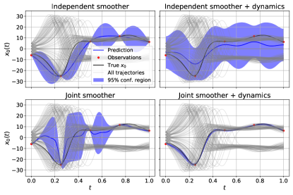
This loss function is a multi-criteria objective, where fitting the data (via the smoother) and identifying the dynamics model (by matching the marginals) regularize each other. In our preliminary experiments, we found the objective to be quite robust w.r.t. different choices of $\lambda$. In the interest of simplicity, we thus set it in all our experiments in Section 4 to a default value of $\lambda=\frac{|\mathcal{D}|}{|\dot{\mathcal{X}}|}$, accounting only for the possibility of having different numbers of supporting points and observations. One special case worth mentioning is $\lambda\rightarrow 0$, which corresponds to conventional sequential smoothing, where the second part would be used for identification in a second step, as proposed by Pillonetto and De Nicolao, (2010). However, as can be seen in Figure 1, the smoother fails to properly identify the system without any knowledge about the dynamics and thus fails to provide meaningful state or derivative estimates. Thus, especially in the case of sparse observations, joint training is strictly superior.

In its final form, unlike its pure Bayesian counterparts, $\operatorname{DGM}$ does not require any prior knowledge about the system dynamics. Nevertheless, if some prior knowledge is available, one could add an additional, additive term $\log(p(\bm{\psi}))$ to $\mathcal{L}(\bm{\varphi},\bm{\psi})$. It should be noted however that this was not done in any of our experiments, and excellent performance can be achieved without.

4 Experiments

We now compare $\operatorname{DGM}$ against state-of-the-art methods. In a first experiment, we demonstrate the effects of an overparametrized, simple dynamics model on the performance of $\operatorname{DGM}$ as well as traditional, MC-based algorithms $\operatorname{SGLD}$ (Stochastic Gradient Lengevin Dynamics, (Welling and Teh,, 2011)) and $\operatorname{SGHMC}$ (Stochastic Gradient Hamiltonian Monte Carlo, (Chen et al.,, 2014)). We select our baselines based on the results of Dandekar et al., (2021), who demonstrate that both a variational approach and $\operatorname{NUTS}$ (No U-Turn Sampler, Hoffman and Gelman, (2014)) are inferior to these two. Subsequently, we will investigate and benchmark the ability of $\operatorname{DGM}$ to correctly identify neural dynamics models and to generalize across different initial conditions. Since $\operatorname{SGLD}$ and $\operatorname{SGHMC}$ reach their computational limits in the generalization experiments, we compare against Neural ODE Processes ($\operatorname{NDP}$). Lastly, we will conclude by demonstrating the necessity of all of its components. For all comparisons, we use the julia implementations of $\operatorname{SGLD}$ and $\operatorname{SGHMC}$ provided by Dandekar et al., (2021), the pytorch implementation of $\operatorname{NDP}$ provided by Norcliffe et al., (2021), and our own JAX (Bradbury et al.,, 2018) implementation of $\operatorname{DGM}$.

4.1 Setup

We use known parametric systems from the literature to generate simulated, noisy trajectories. For these benchmarks, we use the two-dimensional Lotka Volterra (LV) system, the three-dimensional, chaotic Lorenz (LO) system, a four-dimensional double pendulum (DP) and a twelve-dimensional quadrocopter (QU) model. For all systems, the exact equations and ground truth parameters are provided in the Appendix A. For each system, we create two different data sets. In the first, we include just one densely observed trajectory, taking the computational limitations of the benchmarks into consideration. In the second, we include many, but sparsely observed trajectories (5 for LV and DP, 10 for LO, 15 for QU). This setting aims to study generalization over different initial conditions.

4.2 Metric

We use the log likelihood as a metric to compare the accuracy of our probabilistic models. In the 1-trajectory setting, we take a grid of 100 time points equidistantly on the training trajectory. We then calculate the ground truth and evaluate its likelihood using the predictive distributions of our models. When testing for generalization, we repeat the same procedure for unseen initial conditions.

4.3 Effects of Overparametrization

Figure 3: $\operatorname{SGLD}$ does not converge for strongly overparametrized models, the performance of $\operatorname{SGHMC}$ deteriorates. $\operatorname{DGM}$ is not noticeably affected.

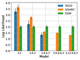
We first study a three-dimensional, linear system of the form $\dot{\bm{x}}(t)=\bm{A}\bm{x}(t)$, where $\bm{A}$ is a randomly chosen matrix with one stable and two marginally stable eigenvalues. For the dynamics model, we choose a linear Ansatz $\bm{f}(\bm{x},\bm{\theta})=\bm{B}\bm{x}(t)$, where $\bm{B}$ is parametrized as the product of multiple matrices. The dimension of the matrices of each factorization are captured in a string of integers of the form $(3,a_{1},\dots,a_{J},3)$. For example, $(3,3)$ corresponds to $\bm{B}$ being just one matrix, while ($3,6,6,3)$ corresponds to $\bm{B}=\bm{B}_{1}\bm{B}_{2}\bm{B}_{3}$, with $\bm{B}_{1}\in\mathbb{R}^{3\times 6}$, $\bm{B}_{2}\in\mathbb{R}^{6\times 6}$ and $\bm{B}_{3}\in\mathbb{R}^{6\times 3}$. All of these models can be interpreted as linear neural networks, forming a simple case of the nonparametric systems we study later. Unlike general neural networks, the expressiveness of the Ansatz is independent of the number of parameters, allowing us to isolate the effects of overparametrization. In Figure 3, we show the mean and standard deviation of the log likelihood of the ground truth over $10$ different noise realizations. The exact procedure for one noise realization is described in the appendix, Appendix C). While $\operatorname{SGLD}$ runs into numerical issues after a medium model complexity, the performance of $\operatorname{SGHMC}$ continuously disintegrates, while $\operatorname{DGM}$ is unaffected. This foreshadows the results of the next two experiments, where we observe that the MC-based approaches are not suitable for the more complicated settings.

Table 1: Log likelihood and prediction times of 100 ground truth sample points, with mean and standard deviation taken over 10 independent noise realizations, for neural ODEs trained on a single, densely sampled trajectory.

	Log Likelihood			Prediction time [ms]
	$\operatorname{DGM}$	$\operatorname{SGHMC}$	$\operatorname{SGLD}$	$\operatorname{DGM}$	$\operatorname{SGHMC}$	$\operatorname{SGLD}$
LV 1	$\mathbf{1.96\pm 0.21}$	$1.36\pm 0.0693$	$1.03\pm 0.0581$	$\mathbf{0.68\pm 0.04}$	$14.98\pm 0.23$	$14.59\pm 0.15$
LO 1	$\mathbf{-0.57\pm 0.11}$	$-3.02\pm 0.158$	$-2.67\pm 0.367$	$\mathbf{0.99\pm 0.05}$	$98.93.\pm 5.79$	$105.03\pm 12.22$
DP 1	$\mathbf{2.13\pm 0.14}$	$1.88\pm 0.0506$	$1.85\pm 0.0501$	$\mathbf{1.31\pm 0.05}$	$10.60\pm 0.21$	$11.34\pm 0.76$
QU 1	$\mathbf{0.64\pm 0.07}$	$-5.00\pm 1.36$	NaN	$\mathbf{3.76\pm 0.12}$	$24.68\pm 6.58$	NaN

4.4 Single Trajectory Benchmarks

In Table 1, we evaluate the log-likelihood of the ground truth for the four benchmark systems, obtained when learning these systems using a neural ODE as a dynamics model (for more details, see appendix B). Clearly, $\operatorname{DGM}$ performs the best on all systems, even though we supplied both $\operatorname{SGLD}$ and $\operatorname{SGHMC}$ with very strong priors and fine-tuned them with an extensive hyperparameter sweep (see Appendix C for more details). Despite this effort, we failed to get $\operatorname{SGLD}$ to work on Quadrocopter 1, where it always returned NaNs. This is in stark contrast to $\operatorname{DGM}$, which performs reliably without any pre-training or priors.

4.5 Prediction speed

To evaluate prediction speed, we consider the task of predicting $100$ points on a previously unseen trajectory. To obtain a fair comparison, all algorithms’ prediction routines were implemented in JAX (Bradbury et al.,, 2018). Furthermore, while we used $1000$ MC samples when evaluating the predictive posterior for the log likelihood to guarantee maximal accuracy, we only used $200$ samples in Table 1. Here, $200$ was chosen as a minimal sample size guaranteeing reasonable accuracy, following a preliminary experiment visualized in Appendix C. Nevertheless, the predictions of $\operatorname{DGM}$ are 1-2 orders of magnitudes faster, as can be seen in Table 1. This further illustrates the advantage of relying on a smoother instead of costly, numerical integration to obtain predictive posteriors in the state space.

Table 2: Log likelihood of 100 ground truth sample points, with mean and covariance taken over 10 independent noise realizations, for neural ODEs trained on a multiple, sparsely sampled trajectory.The number following the system name denotes the number of trajectories in the training set.

	Log Likelihood
	$\operatorname{DGM}$	$\operatorname{NDP}$
LV 100	$\mathbf{1.81\pm 0.08}$	$0.62\pm 0.27$
LO 125	$\mathbf{-2.18\pm 0.76}$	$-2.85\pm 0.05$
DP 100	$\mathbf{1.86\pm 0.05}$	$0.88\pm 0.05$
QU 64	$\mathbf{-0.54\pm 0.36}$	$-0.91\pm 0.07$

Figure 4: Log likelihood of the ground truth for Lotka Volterra for increasing number of trajectories with 5 observations each.

4.6 Multi-Trajectory Benchmarks

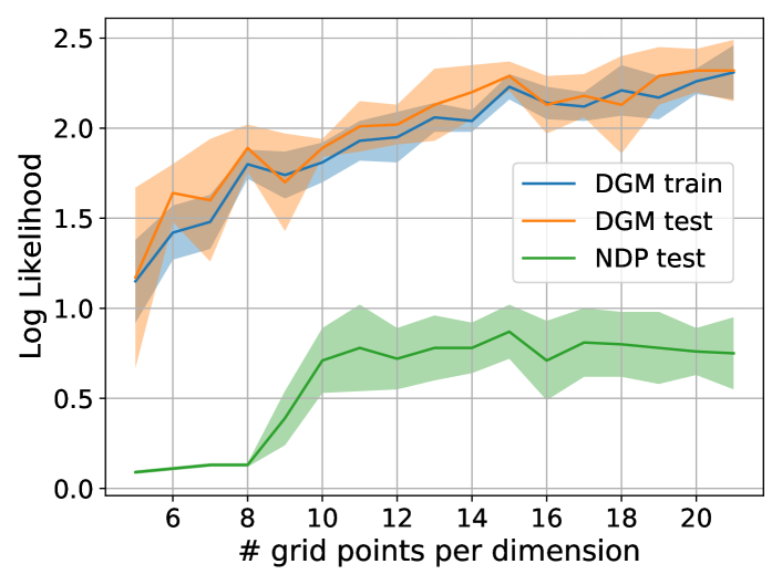
Next, we take a set of trajectories starting on an equidistant grid of the initial conditions. Each trajectory is then observed at $5$ equidistant observation times for LV and DP, and $10$ equidistant observation times for the chaotic Lorenz and more complicated Quadrocopter. We test generalization by randomly sampling a new initial condition and evaluating the negative log likelihood of the ground truth at $100$ equidistant time points. In Table 2, we compare the generalization performance of $\operatorname{DGM}$ against $\operatorname{NDP}$, since despite serious tuning efforts, the MC methods failed to produce meaningful results in this setting. $\operatorname{DGM}$ clearly outperforms $\operatorname{NDP}$, a fact which is further exemplified in Figure 4. There, we show the test log likeliood for Lotka Volterra trained on an increasing set of trajectories. Even though the time grid is fixed and we only decrease the distance between initial condition samples, the dynamics model helps the smoother to generalize across time as well. In stark contrast, $\operatorname{NDP}$ fails to improve with increasing data after an initial jump.

4.7 Ablation study

We next study the importance of different elements of our approach via an ablation study on the Lorenz 125 dataset, shown in Figure 1. Comparing the two rows, we see that joint smoothing across trajectories is essential to transfer knowledge between different training trajectories. Similarly, comparing the two columns, we see that the dynamics model enables the smoother to reduce its uncertainty in between observation points.

4.8 Computational Requirements

For the one trajectory setting, all $\operatorname{DGM}$ related experiments were run on a Nvidia RTX 2080 Ti, where the longest ones took 15 minutes. The comparison methods were given 24h, on Intel Xeon Gold 6140 CPUs. For the multi-trajectory setting, we used Nvidia Titan RTX, where all experiments finished in less than 3 hours. A more detailed run time compilation can be found in Appendix B. Using careful implementation, the run time of $\operatorname{DGM}$ scales linearly in the number of dimensions $K$. However, since we use an accurate RBF kernel for all our experiments reported in this section, we have cubic run time complexity in $\sum_{m=1}^{M}N_{m}$. In principle, this can be alleviated by deploying standard feature approximation methods (Rahimi et al.,, 2007; Liu et al.,, 2020). While this is a well known fact, we nevertheless refer the interested reader to a more detailed discussion of the subject in Appendix D.

5 Related work

5.1 Bayesian Parameter Inference with Gaussian Processes

The idea of matching gradients of a (spline-based) smoother and a dynamics model goes back to the work of Varah, (1982). For GPs, this idea is introduced by Calderhead et al., (2009), who first fit a GP to the data and then match the parameters of the dynamics. Dondelinger et al., (2013) introduce concurrent training, while Gorbach et al., (2017) introduce an efficient variational inference procedure for systems with a locally-linear parametric form. All these works claim to match the distributions of the gradients of the smoother and dynamics models, by relying on a product of experts heuristics. However, Wenk et al., (2019) demonstrate that this product of experts in fact leads to statistical independence between the observations and the dynamics parameters, and that these algorithms essentially match point estimates of the gradients instead. Thus, $\operatorname{DGM}$ is the first algorithm to actually match gradients on the level of distributions for ODEs. In the context of stochastic differential equations (SDEs) with constant diffusion terms, Abbati et al., (2019) deploy MMD and GANs to match their gradient distributions. However, it should be noted that their algorithm treats the parameters of the dynamics model deterministically and thus, they can not provide the epistemic uncertainty estimates that we seek here. Note that our work is not related to the growing literature investigating SDE approximations of Bayesian Neural ODEs in the context of classification (Xu et al.,, 2021). Similarly to Chen et al., (2018), these works emphasize learning a terminal state of the ODE used for other downstream tasks.

5.2 Gaussian Processes with Operator Constraints

Gradient matching approaches mainly use the smoother as a proxy to infer dynamics parameters. This is in stark contrast to our work, where we treat the smoother as the main model used for prediction. While the regularizing properties of the dynamics on the smoother are explored by Wenk et al., (2020), Jidling et al., (2017) introduce an algorithm to incorporate linear operator constraints directly on the kernel level. Unlike in our work, they can provide strong guarantees that the posterior always follows these constraints. However, it remains unclear how to generalize their approach to the case of complex, nonlinear operators, potentially parametrized by neural dynamics models.

5.3 Other Related Approaches

In some sense, the smoother is mimicking a probabilistic numerical integration step, but without explicitly integrating. In spirit, this approach is similar to the solution networks used in the context of PDEs, as presented by Raissi et al., (2019), which however typically disregard uncertainty. In the context of classical ODE parameter inference, Kersting et al., (2020) deploy a GP to directly mimic a numerical integrator in a probabilistic, differentiable manner. Albeit promising in a classical, parametric ODE setting, it remains unclear how these methods can be scaled up, as there is still the numerical integration bottleneck. Unrelated to their work, Ghosh et al., (2021) present a variational inference scheme in the same, classical ODE setting. However, they still keep distributions over all weights of the neural network (Norcliffe et al.,, 2021). A similar approach is investigated by Dandekar et al., (2021), who found it to be inferior to the MC methods we use as a benchmark. Variational inference was previously employed by Yildiz et al., (2019) in the context of latent neural ODEs parametrized by a Bayesian neural network, but their work mainly focuses on dimensionality reduction. Nevertheless, their work inspired a model called Neural ODE Processes by Norcliffe et al., (2021). This work is similar to ours in the sense that it avoids keeping distributions over network weights and models an ensemble of deterministic ODEs via a global context variable. Consequently, we use it as a benchmark in Section 4, showing that it does not properly capture epistemic uncertainty in a low data setting, which might be problematic for downstream tasks like reinforcement learning.

6 Conclusion

In this work, we introduced a novel, GP-based collocation method, that matches gradients of a smoother and a dynamics model on the distribution level using a Wasserstein loss. Through careful parametrization of the dynamics model, we manage to train complicated, neural ODE models, where state of the art methods struggle. We then demonstrate that these models are able to accurately predict unseen trajectories, while capturing epistemic uncertainty relevant for downstream tasks. In future work, we are excited to see how our training regime can be leveraged in the context of active learning of Bayesian neural ordinary differential equation for continuous-time reinforcement learning.

.tocmtappendix mtchapternone mtappendixsubsection

Appendix A Dataset description

In this section, we describe the datasets we use in our experiments.

A.1 Lotka Volterra

The two dimensional Lotka Volterra system is governed by the parametric differential equations

$$\frac{dx}{dt} =\alpha x-\beta xy$$

$$\frac{dy}{dt} =\delta xy-\gamma y,$$

where we selected $(\alpha,\beta,\gamma,\delta)=(1,1,1,1)$. These equations were numerically integrated to obtain a ground truth, where the initial conditions and observation times depend on the dataset. All observations were then created by adding additive, i.i.d. noise, distributed according to a normal distribution $\mathcal{N}\left(|0,0.1^{2}\right)$.

LV 1 consists of one trajectory starting from initial condition $(1,2)$. The trajectory is observed at $100$ equidistant time points from the interval $(0,10)$.

LV 100 consists of 100 trajectories. Initial conditions for these trajectories are located on a grid, i.e.,

$$\left\{\left(\frac{1}{2}+\frac{i}{9},\frac{1}{2}+\frac{j}{9}\right)\Big{|}i\in\{0,\dots,9\},j\in\{0,\dots,9\}\right\}.$$

Each trajectory is then observed at $5$ equidistant time points from the interval $(0,10)$, which leads to a total of $500$ observations.

Figure 5: The first row represents the true states and all observations of LV 1 with random seed 0. In the second row we plot all ground truth trajectories from the dataset LV 100. One particular trajectory is highlighted in black, together with the corresponding observations of that trajectory (red dots).

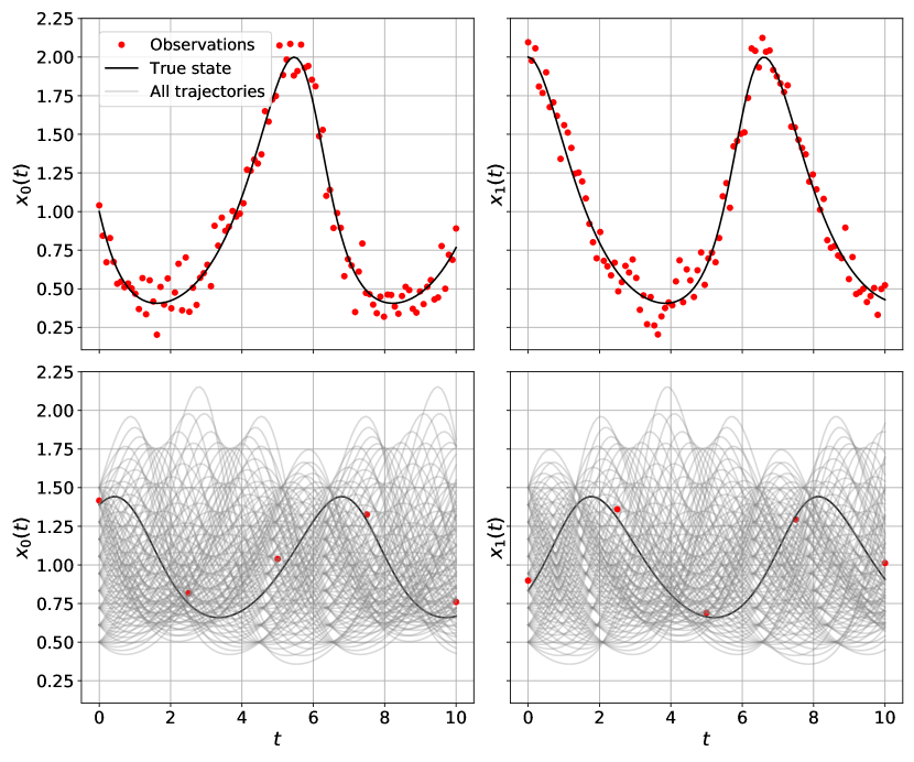
To test generalization, we created $10$ new trajectories. The initial conditions of these trajectories were obtained by sampling uniformly at random on $[0.5,1.5]^{2}$. To evaluate the log likelihood, we used $100$ equidistant time points from the interval $(0,10)$.

A.2 Lorenz

The 3 dimensional, chaotic Lorenz system is governed by the parametric differential equations

$$\frac{dx}{dt}=\sigma(y-x)$$

$$\frac{dy}{dt}=x(\rho-z)-y$$

$$\frac{dz}{dt}=xy-\tau y,$$

where we selected $(\sigma,\rho,\tau)=(10,28,8/3)$. These equations were numerically integrated to obtain a ground truth, where the initial conditions and observation times depend on the dataset. All observations were then created by adding additive, i.i.d. noise, distributed according to a normal distribution $\mathcal{N}\left(|0,1\right)$.

LO 1 consists of one trajectory starting from initial condition $(-2.5,2.5,2.5)$. The trajectory is observed at $100$ equidistant time points from the interval $(0,1)$.

LO 125 consists of 125 trajectories. Initial conditions for these trajectories are located on a grid, i.e.,

$$\left\{\left(-5+\frac{5i}{2},-5+\frac{5j}{2},-5+\frac{5k}{2}\right)\Big{|}i\in\{0,\dots,4\},j\in\{0,\dots,4\},k\in\{0,\dots,4\}\right\}.$$

Each trajectory is then observed on $10$ equidistant time points from the interval $(0,1)$, which leads to a total of $1250$ observations.

Figure 6: The first row represents the true states and all observations of LO 1 with random seed 0. In the second row we plot all ground truth trajectories from the dataset LO 125. One particular trajectory is highlighted in black, together with the corresponding observations of that trajectory (red dots).

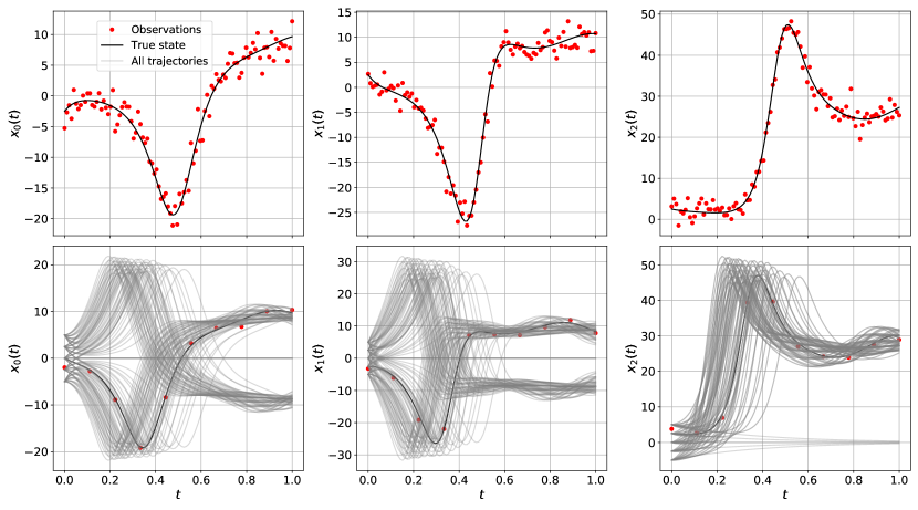
To test generalization, we created $10$ new trajectories. The initial conditions of these trajectories were obtained by sampling uniformly at random on $[-5,5]^{3}$. To evaluate the log likelihood, we used $100$ equidistant time points from the interval $(0,1)$.

A.3 Double Pendulum

The $4$ dimensional Double pendulum system is governed by the parametric differential equations

$${\dot{\theta}_{1}} =\frac{6}{ml^{2}}\frac{2p_{\theta_{1}}-3\cos(\theta_{1}-\theta_{2})p_{\theta_{2}}}{16-9\cos^{2}(\theta_{1}-\theta_{2})}$$

$${\dot{\theta}_{2}} =\frac{6}{ml^{2}}\frac{8p_{\theta_{2}}-3\cos(\theta_{1}-\theta_{2})p_{\theta_{1}}}{16-9\cos^{2}(\theta_{1}-\theta_{2})}.$$

$${\dot{p}_{\theta_{1}}} =-\tfrac{1}{2}ml^{2}\left({\dot{\theta}_{1}}{\dot{\theta}_{2}}\sin(\theta_{1}-\theta_{2})+3\frac{g}{l}\sin\theta_{1}\right)$$

$${\dot{p}_{\theta_{2}}} =-\tfrac{1}{2}ml^{2}\left(-{\dot{\theta}_{1}}{\dot{\theta}_{2}}\sin(\theta_{1}-\theta_{2})+\frac{g}{l}\sin\theta_{2}\right),$$

where we selected $(g,m,l)=(9.81,1,1)$. In these equations, $\theta_{1}$ and $\theta_{2}$ represent the offset angles, while $p_{\theta_{1}}$ and $p_{\theta_{1}}$ represent the momentum of the upper and lower pendulum. These equations were numerically integrated to obtain a ground truth, where the initial conditions and observation times depend on the dataset.

Figure 7: Double Pendulum where both rods have equal length and mass.

All observations were then created by adding additive, i.i.d. noise, distributed according to a normal distribution $\mathcal{N}\left(|0,0.1^{2}\right)$.

DP 1 consist of one trajectory starting from initial condition $(-\pi/6,-\pi/6,0,0)$. The trajectory is observed at $100$ equidistant time points from the interval $(0,1)$.

DP 100 consists of 100 trajectories. Initial conditions for these trajectories are located on a grid, i.e.,

$$\left\{\left(-\frac{\pi}{6}+\frac{\pi i}{27},-\frac{\pi}{6}+\frac{\pi j}{27},0,0\right)\Big{|}i\in\{0,\dots,9\},j\in\{0,\dots,9\}\right\}.$$

Each trajectory is then observed at $5$ equidistant time points from the interval $(0,1)$, which leads to a total of $500$ observations.

Figure 8: The first row represents the true states and all observations of DP 1 with random seed 0. In the second row we plot all ground truth trajectories from the dataset DP 100. One particular trajectory is highlighted in black, together with the corresponding observations of that trajectory (red dots).

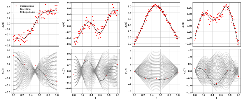
To test generalization, we created $10$ new trajectories. The initial conditions of these trajectories were obtained by sampling uniformly at random on $[-\frac{\pi}{6},\frac{\pi}{6}]^{2}\times\{0\}^{2}$. To evaluate the log likelihood, we used $100$ equidistant time points from the interval $(0,1)$.

A.4 Quadrocopter

The $12$ dimensional Quadrocopter system is governed by the parametric differential equations

$$\dot{u} =-g\sin(\theta)+rv-qw$$

$$\dot{v} =g\sin(\phi)\cos(\theta)-ru+pw$$

$$\dot{w} =-F_{z}/m+g\cos(\phi)\cos(\theta)+qu-pv$$

$$\dot{p} =\left(L+(I_{yy}-I_{zz})qr\right)/I_{xx}$$

$$\dot{q} =\left(M+(I_{zz}-I_{xx})pr\right)/I_{yy}$$

$$\dot{r} =(I_{xx}-I_{yy})pq/I_{zz}$$

$$\dot{\phi} =p+(q\sin(\phi)+r\cos(\phi))\tan(\theta)$$

$$\dot{\theta} =q\cos(\phi)-r\sin(\phi)$$

$$\dot{\psi} =(q\sin(\phi)+r\cos(\phi))\sec(\theta)$$

$$\dot{x} =\cos(\theta)\cos(\psi)u+(-\cos(\phi)\sin(\psi)+\sin(\phi)\sin(\theta)\cos(\psi))v+$$

$$+(\sin(\phi)\sin(\psi)+\cos(\phi)\sin(\theta)\cos(\phi))w$$

$$\dot{y} =\cos(\theta)\sin(\psi)u+(\cos(\phi)\cos(\psi)+\sin(\phi)\sin(\theta)\sin(\psi))v+$$

$$+(-\sin(\phi)\cos(\psi)+\cos(\phi)\sin(\theta)\sin(\phi))w$$

$$\dot{z} =\sin(\theta)u-\sin(\phi)\cos(\theta)v-\cos(\phi)\cos(\theta)w,$$

where

$$F_{z} =F_{1}+F_{2}+F_{3}+F_{4}$$

$$L =(F_{2}+F_{3})d_{y}-(F_{1}+F_{4})d_{x}$$

$$M =(F_{1}+F_{3})d_{x}-(F_{2}+F_{4})d_{x}.$$

We fixed the input control forces to $(F_{1},F_{2},F_{3},F_{4})=(0.496,0.495,0.4955,0.4955)$ (not to be inferred) and selected $(m,I_{xx},I_{yy},I_{zz},d_{x},d_{y},g)=(0.1,0.62,1.13,0.9,0.114,0.0825,9.85)$. These equations were numerically integrated to obtain a ground truth, where the initial conditions and observation times depend on the dataset. All observations were then created by adding additive, i.i.d. noise, distributed according to a normal distribution $\mathcal{N}\left(|0,\Sigma\right)$, where

$$\Sigma=\operatorname{diag}(1,1,1,0.1,0.1,0.1,1,0.1,0.1,5,5,5).$$

QU 1 consists of one trajectory starting from initial condition $(0,0,0,0,0,0,0,0,0,0,0,0)$. The trajectory is observed at $100$ equidistant time points from the interval $(0,10)$.

QU 64 consists of $64$ trajectories. Initial conditions for these trajectories are located on a grid, i.e.,

$$\left\{\left(0,0,0,0,0,0,-\frac{\pi}{18}+\frac{\pi i}{27},-\frac{\pi}{18}+\frac{\pi j}{27},-\frac{\pi}{18}+\frac{\pi k}{27},0,0,0\right)\Big{|}(i,j,k)\in\{0,\dots,4\}^{3}\right\}.$$

Each trajectory is then observed at $15$ equidistant time points from the interval $(0,10)$, which leads to a total of $960$ observations.

Figure 9: Visualization showing the true states and all observations of QU 1 with random seed 0.

Figure 10: Visualization showing all ground truth trajectories from the dataset QU 64. One particular trajectory is highlighted in black, together with the corresponding observations of that trajectory (red dots).

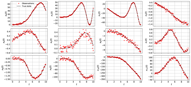
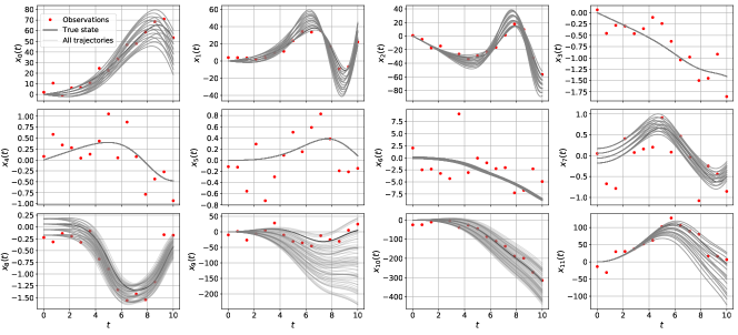
To test generalization, we created $10$ new trajectories. The initial conditions of these trajectories were obtained by sampling uniformly at random on $\{0\}^{6}\times[-\frac{\pi}{18},\frac{\pi}{18}]^{2}\times\{0\}^{3}$. To evaluate the log likelihood, we used $100$ equidistant time points from the interval $(0,10)$.

Appendix B Implementation details of $\operatorname{DGM}$

In this section we discuss all implementation details of $\operatorname{DGM}$. As described in Section 3, $\operatorname{DGM}$ consists of a smoother and a dynamics model. At training time, the dynamics model is then used to regularize the smoother via the squared type-2 Wasserstein distance.

B.1 Dynamics model

The role of the dynamics model is to map every state $\bm{x}$ to a distribution over derivatives, which we decide to parameterize as $\mathcal{N}\left(|\bm{f}(\bm{x},\bm{\psi}),\bm{\Sigma}_{D}(\bm{x},\bm{\psi})\right)$. In the paper we focused in the case where we do not have any prior knowledge about the dynamics and we model both $\bm{f}$ and $\bm{\Sigma}_{D}$ with neural network. Nevertheless, if some prior knowledge about the dynamics $\bm{f}$ is available, it can be used to inform the mean function $\bm{f}$ (potentially also covariance $\bm{\Sigma}_{D}$) appropriately. In particular, if the parametric form of the dynamics is known, we can use them as a direct substitute for $\bm{f}$. This is the special case of ODE-parameter inference, which we investigate empirically in Appendix E. Next we present implementation details of both non-parametric (i.e. $\bm{f}$ given by a neural network) and parametric (i.e. $\bm{f}$ given by some parametric form) dynamics models.

Non-parametric dynamics

In the non-parametric case, we model both the dynamics’ mean function $\bm{\mu}_{D}$ and covariance function $\bm{\Sigma}_{D}$ with a neural networks. Across all experiments, we choose a simple 3-layer neural network with 20, 20 and $2n$ nodes, where $n$ denotes the number of state dimensions of a specific system. After each layer, we apply the sigmoid activation function, except for the last one. The first $n$ output nodes represent the mean function. Here, no activation function is necessary for the last layer. The second $n$ output nodes are used to construct the diagonal covariance $\bm{\Sigma}_{D}$. To ensure positivity, we use $x\mapsto\log(1+\exp(x))^{2}$ as an activation function on the last $n$ nodes of the last layer.

Parametric dynamics

In the parametric case, we model $\bm{\mu}_{D}$ using the parametric form of the vector field. Across all experiments, we choose a simple 3-layer neural network with 10, 10 and $n$ nodes, where $n$ denotes the number of state dimensions of a specific system. After each lyer, we apply the sigmoid activation function, except for the last one. The $n$ nodes are then used to construct the diagonal covariance $\bm{\Sigma}_{D}$. To ensure positivity, we use $x\mapsto\log(1+\exp(x))^{2}$ as an activation function on the last layer.

B.2 Smoother model

The role of the smoother model is to map every tuple $(\bm{x}(0),t)$ consisting of initial condition $\bm{x}(0)$ and time $t$ to $\bm{x}(t)$, which is the state at time $t$ of a trajectory starting at $\bm{x}(0)$ at time $0$. In the paper, we model the smoother using a Gaussian process with a deep mean function $\bm{\mu}$ and a deep feature map $\phi$. Both of them take as input the tuple $(\bm{x}(0),t)$. This tuple is then mapped through a dense neural network we call core. For all experiments, we chose a core with two layers, with 10 and 5 hidden nodes and sigmoid activation on both. The output of the core is then fed into two linear heads. The head for $\bm{\mu}$ builds a linear combination of the core’s output to obtain a vector of the same shape as $\bm{x}(t)$. The head for $\phi$ builds a linear combination of the core’s output to obtain a vector of length $3$, the so called features. These features are then used as inputs to a standard RBF kernel with ARD (Rasmussen,, 2004). For each state dimension, we keep a separate $\phi$-head, as well as separate kernel hyperparameters. However, the core is shared across dimensions, while $\bm{\mu}$ is directly introduced as multidimensional.

In the paper, we set the variance of the RBF to $1$ and learned the lengthscales together with all other hyperparameters. However, due to the expressiveness of the neural network, the lengthscales are redundant and could easily be incorporated into the linear combination performed by the head. Thus, in the scaling experiments, we fix the lengthscale to one and approximate the RBF kernel with a feature expansion, as detailed in Appendix D.

B.3 Evaluation metric

To evaluate the quality of our models’ predictions, we use the log likelihood. To obtain the log likelihood, we first use the model to predict the mean and standard deviation at 100 equidistant times. Then we calculate the log likelihood of the ground truth for every predicted point. We take the mean over dimensions, over times, and over trajectories. When reporting the training log likelihood, as done e.g. in Table 1, we use the training trajectories for evaluation. When reporting the generalization log likelihood, as done e.g. in Table 2, we use $10$ unseen trajectories. This evaluation is then repeated for $10$ different , meaning that we retrain the model $10$ times on a data set with the same ground truth, but a different noise realization. We then report the mean and standard deviation of the log likelihood across these repetitions.

Weight decay

To prevent overfitting, we use weight decay on the parameters of both the dynamics and the smoother neural networks. We denote by $wd_{D}$ the weight decay parameter of the dynamics model, and $wd_{S}$ the weight decay parameters of the smoother model. While we keep the $wd_{S}$ constant during all three phases of training, we gradually increase $wd_{D}$ from $0$ to its final value, which is the same as $wd_{S}$. The increase follows a polynomial schedule with power $0.8$.

B.4 Training details

The training of $\operatorname{DGM}$, i.e. optimizing Equation 5, can be split into three distinct phases: transition, training, and fine-tuning. In the transition phase we gradually increase the value of both $\lambda$ and the weight decay regularization parameter of the dynamics $(wd_{D})$ from 0 to its final value. When these parameters reach their final value, we reach the end of the transition phase and start the training phase. In this phase, all optimization parameters are left constant. It stops when the last $1000$ steps are reached. Then, the fine-tune phase starts, where we decrease learning rate to $0.01$. The gradual increase of $\lambda$ and $wd_{D}$ follows polynomial schedule with power $0.8$. As an optimizer, we use Adam.

Supporting points

The selection of the supporting points in $\mathcal{T}$ is different for data sets consisting of one or multiple trajectories. If there is only one trajectory in the dataset, we match the derivatives at the same places where we observe the state. If there are multiple trajectories, we match the derivatives at $30$ equidistant time points on each training trajectory.

Selection of $\lambda$

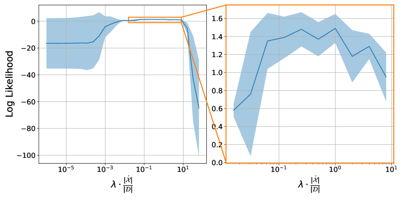
The loss of Equation 5 is a multi-objective optimization problem with a trade-off parameter $\lambda$. Intuitively, if $\lambda$ is too small, the model only tries to fit the data and neglects the dynamics. On the other hand, with too large $\lambda$, the model neglects the data fit and only cares about the dynamics. In Figure 11 we show a plot of log likelihood score on the $10$ test trajectories of the LV 100 dataset with varying $\lambda$. We train the model for $\lambda\cdot|\dot{\mathcal{X}}|/|\mathcal{D}|\in\{2^{i}|i=-20,\ldots,6\}$. To estimate the robustness of the experiment, we show the mean and standard deviation over $5$ different noise realizations.

Figure 11: If $\lambda$ is too small, the dynamics model does not regularize the smoother sufficiently, the model overfits to the data and the test log likelihood score is worse. If $\lambda$ is too large, the observation term gets dominated, the model underfits and the log likelihood score on the test data is worse. Empirically, we found that we achieve the best log likelihood on the test data with $\lambda=|\mathcal{D}|/|\dot{\mathcal{X}}|$.

Parameter selection

To search for the best performing parameters we performed sweep over learning rate value $lr$ in the transition and training phase and over the weight decay parameters $wd_{S}$. For $lr$, we considered the values $0.02,0.05$ and $0.1$. For $wd_{S}$, we considered $0.1,0.5$ and $1.0$.

Training time

We did not optimize our hyperparameters and code for training time. Nevertheless, we report the length of each phase and the total time in the Table 3.

Table 3: Number of steps for each training phase and total training time for different datasets. For the times, we report mean $\pm$ standard deviation over 10 different random seeds.

	Transition	Training	Fine-Tuning	Time[s]
LV 1	1000	0	1000	$329\pm 15$
LO 1	1000	0	1000	$399\pm 6$
DP 1	1000	1000	1000	$535\pm 42$
QU 1	1000	2000	1000	$1121\pm 41$
LV 100	1000	0	1000	$408\pm 8$
LO 125	1000	0	1000	$753\pm 8$
DP 100	5000	4000	1000	$2988\pm 261$
QU 64	6000	3000	1000	$8387\pm 36$

Appendix C Bayesian NODE training

In this section, we describe the specifics of the experiments and the implementation of $\operatorname{SGLD}$ and $\operatorname{SGHMC}$, the Bayesian integration benchmarks used in the paper. For all experiments, we use a slightly changed version of the code provided by Dandekar et al., (2021), which is written in Julia (Bezanson et al.,, 2017).

C.1 Effects of Overparametrization

Here we provide further details regarding the experiment presented in Figure 3. For the ground truth dynamics $\dot{\bm{x}}=\bm{A}\bm{x}$, we selected the matrix $\bm{A}$ such that it has $1$ stable and $2$ marginally stable modes. The eigenvalue of the stable mode is selected uniformly at random from $[-0.5,-0.1]$. To create marginally stable modes, we create a block $\bm{C}\in\mathbb{R}^{2\times 2}$, where its components are sampled i.i.d. uniformly at random from $[0,1]$. The marginally stable part is then created as $\bm{A}$ as $\frac{\pi}{2\rho(\bm{C}-\bm{C}^{\top})}\left(\bm{C}-\bm{C}^{\top}\right)$, where $\rho(.)$ denotes the spectral radius. Using the spectral radius in the normalization ensures that the period of the mariginally stable mode is bounded with $\pi/2$. We selected the initial condition for the trajectory uniformly at random from the unit sphere in $\mathbb{R}^{3}$. We evolved the trajectory on the time interval $(0,10)$ and observed 100 noisy observations, where every ground truth value was perturbed with additive, independent Gaussian noise, drawn from $\mathcal{N}\left(|0,0.1^{2}\right)$.

While $\operatorname{DGM}$ performed without any pre-training, we observed that both $\operatorname{SGLD}$ and $\operatorname{SGHMC}$ struggle without narrow priors. To obtain reasonable priors, we followed the following procedure:

First, we pretrain every set of matrices $\bm{B}_{1},\dots,\bm{B}_{k}$ on the ground truth, such that the

$$\sum_{i=1}^{100}\left\lVert\dot{\bm{x}}(t_{i})-\prod_{j=1}^{k}\bm{B}_{j}\bm{x}(t_{i})\right\rVert_{2}^{2}\leq 10^{-5},$$

where $t_{i}$ are times at which we observed the state. We selected the prior as Gaussian centered around the pretrained parameters. The standard deviation was chosen such that the standard deviation of the product of the matrices $\prod_{j=1}^{k}\bm{B}_{j}$ stays at $0.01$, independent of the number of matrices used. For $\operatorname{SGHMC}$, we selected learning rate $1.5\times 10^{-7}$ and momentum decay $0.1$ as hyperparameters. For $\operatorname{SGLD}$,we chose the hyperparameters $a=0.001,b=1$ and $\gamma=0.9$, which $\operatorname{SGLD}$ then uses to calculate a polynomial decay $a(b+k)^{-\gamma}$ (at step $k$) for its learning rate. For sampling we used $5$ chains with $20000$ samples on each chain. The last $2000$ samples of each chain were used for evaluation. With this setting we ensured that the $r$-hat score was smaller than 1.1.

C.2 Finetuning for Benchmark Systems

Both $\operatorname{SGLD}$ and $\operatorname{SGHMC}$ require hyperparameters, that influence their performance quite strongly. In this subsection, we explain all the tuning steps and requirements we deployed for these algorithms to produce the results shown in the main paper. For both algorithms, we used a setup of $6$ chains, that were sampled in parallel, with $10000$ samples per chain, where the final $2000$ samples were taken as predictions. These numbers were selected using the r-hat value to determine if the chains had sufficiently converged.

Hyperparameters of $\operatorname{SGLD}$

For $\operatorname{SGLD}$, we additionally searched over the hyperparameters $a$, $b$, and $\gamma$. All three are used to calculate the learning rate of the algorithm. These parameters were chosen by evaluating the log likelihood of the ground truth on a grid, which was given by the values $a\in\{0.0001,0.001,0.005,0.01,0.05,0.1\}$, $b\in\{0.3,0.6,1.0,1.5,2\}$ and $\gamma\in\{0.5001,0.55,0.6,0.7,0.8,0.99\}$. Clearly, using the log likelihood of the ground truth to tune the hyperparameters overestimates the performance of the algorithm, but it provides us with an optimistic estimate of its real performance in practice. For computational reasons, we only performed a grid search on the one trajectory experiments, and then reused the same hyperparameters on the multi-trajectory experiments. All hyperparameters are shown in Table 4.

Hyperparameters of $\operatorname{SGHMC}$

For $\operatorname{SGHMC}$, we additionally searched over the hyperparameters the learning rate and the momentum decay. Again, these parameters were chosen by evaluating the log likelihood of the ground truth on a grid, where learning rate was chosen from the set $\{1\mathrm{e}{-8},5\mathrm{e}{-8},1.5\mathrm{e}{-7},5\mathrm{e}{-7},1\mathrm{e}{-6},5\mathrm{e}{-6},1\mathrm{e}{-5},5\mathrm{e}{-5},1\mathrm{e}{-4},5\mathrm{e}{-4}\}$ and momentum decay was chosen from the set $\{0.0001,0.001,0.05,0.1,0.5,1,5\}$. Since we used the log likelihood of the ground truth again to tune the hyperparameters, we overestimate the performance of the algorithm and obtain thus an optimistic estimate of its real performance in practice. For computational reasons, be only performed a grid search on the one trajectory experiments, and then reused the same hyperparameters on the multi-trajectory experiments. All hyperparameters are shown in Table 4.

Table 4: Hyperparameters with best performance evaluated on the likelihood of the ground truth. The hyperparameters are different for the parametric (p) and the non-parametric (n) dynamics models, which is indicated with the last letter.

	$\operatorname{SGLD}$			$\operatorname{SGHMC}$
	$a$	$b$	$\gamma$	learning rate	momentum decay
Lotka Volterra p	$1\mathrm{e}{-3}$	$2$	$0.5001$	$5\mathrm{e}{-7}$	$0.1$
Lorenz p	$0.001$	$1.5$	$0.5001$	$1\mathrm{e}{-5}$	$0.05$
Double Pendulum p	$0.1$	$0.3$	$0.5001$	$1\mathrm{e}{-6}$	$0.1$
Quadrocopter p	$0.0001$	$1.5$	$0.7$	$5\mathrm{e}{-7}$	$0.5$
Lotka Volterra n	$0.005$	$1.5$	$0.7$	$5\mathrm{e}{-7}$	$0.5$
Lorenz n	$0.001$	$1.5$	$0.55$	$5\mathrm{e}{-6}$	$0.1$
Double Pendulum n	$0.01$	$2$	$0.55$	$1\mathrm{e}{-6}$	$0.05$
Quadrocopter n	F	F	F	$5\mathrm{e}{-7}$	$0.05$

Choice of Priors for $\operatorname{SGLD}$ and $\operatorname{SGHMC}$

Since $\operatorname{SGLD}$ and $\operatorname{SGHMC}$ are both Bayesian methods, they need to be supplied with a prior. As we discovered in our experiments, this prior plays a crucial role in the stability of the algorithm. In the end, we did not manage to get them to converge without some use of ground truth. In particular, if the priors were not chosen narrowly around some ground truth, the algorithms just returned NaNs, since their integration scheme runs into numerical issues. For the parametric case shown in Appendix E, where we assume access to the true parametric form of the system, we thus chose narrow priors around the ground truth of the parameter values, that were used to create the data set. For Lotka Volterra, we chose a uniform distribution around the ground truth $\pm 0.5$, i.e. $\theta_{i}\sim\textrm{Uniform}[0.5,1]$ for all components of $\bm{\theta}$. For Lorenz, we chose $\alpha\sim\textrm{Uniform}[8,12]$, $\beta\sim\textrm{Uniform}[25,31]$ and $\gamma\sim\textrm{Uniform}[6/3,10/3]$. For Double Pendulum, we chose $m\sim\textrm{Uniform}[0.5,1.5]$ and $l\sim\textrm{Uniform}[0.5,1.5]$. For Quadrocopter, we chose independent Gaussians, centered around the ground truth, with a standard deviation of $0.005$. For all experiments, the prior on the observation noise was set to $\sigma\sim\mathrm{InverseGamma}[2,3]$, except for $\operatorname{SGLD}$ when inferring the Lorenz system. There, we had to fix the noise standard deviation to its ground truth, to get convergence.

For the non-parametric case shown in the main paper, we needed a different strategy, since no ground truth information was available for the weights of the neural dynamics model. Thus, we first trained a deterministic dynamics model. As data, we sampled $100$ tuples $\bm{x},\dot{\bm{x}}$ equidistantly in time on the trajectory. Note that we implicitly assume access to the ground truth of the dynamics model, i.e. we assume we are provided with accurate, noise free $\dot{\bm{x}}$. The neural dynamics model was then pre-trained on these pairs, until the loss was almost zero (up to $1\mathrm{e}{-5}$). $\operatorname{SGLD}$ and $\operatorname{SGHMC}$ were then provided with Gaussian priors, independent for each component of $\bm{\theta}$, centered around the pre-trained weights, with a standard deviation of 0.1.

C.3 Number of integrations for prediction

$\operatorname{SGLD}$ and $\operatorname{SGHMC}$ both return samples of the parameters of the dynamics model. To obtain uncertainties in the state space at prediction time, each one of these samples needs to be turned into a sample trajectory, by using numerical integration. To obtain maximum accuracy, we would ideally integrate all parameter samples obtained by the chains. However, due to the computational burden inflicted by numerical integration, this is not feasible. We thus need to find a trade-off between accuracy and computational cost, by randomly subsampling the number of available parameter samples.

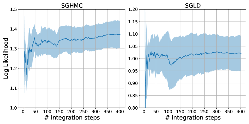
In Figure 12 we show how the log likelihood of the ground truth changes with increasing number of sample trajectories on the LV 1 dataset. After initial fluctuations, the log likelihood of the ground truth stabilizes after approximately $200$ steps. To obtain the results of Table 1, we thus chose $200$ integration steps.

Figure 12: We select the number of sample trajectories for uncertainty prediction to be $200$, since we observe that the log likelihood of the ground truth stops fluctuating after $200$ steps.

Appendix D Scaling to many observations or trajectories

Let $N$ be the total number of observations, summed over all training trajectories. In this section, we will analyze the computational complexity of $\operatorname{DGM}$ in terms of $N$ and demonstrate how this can be drastically reduced using standard methods from the literature. For notational compactness, we will assume that the supporting points in $\mathcal{T}$ are at the same locations as the observations in $\mathcal{D}$. However, this is by no means necessary. As long as they are chosen to be constant or stand in a linear relationship to the number of observations, our analysis still holds. We will thus use $\bm{x}$ and $\bm{x}_{\text{supp}}$ and the corresponding quantities interchangeably. Similarly, we will omit the $k$ that was used for indexing the state dimension and assume one-dimensional systems. The extension to multi-dimensional systems is straight forward and comes at the cost of an additional factor $K$.

Fortunately, most components of the loss of $\operatorname{DGM}$ given by Equation 5 can be calculated in linear time. In particular, it is worth noting that the independence assumption made when calculating the Wasserstein distance in Section 3.4 alleviates the need to work with the full covariance matrix and lets us work with its diagonal elements instead. Nevertheless, there are several terms that are not straight forward to calculate. Besides the marginal log likelihood of the observations, these are the posteriors

$$p_{S}(\bm{x}|\mathcal{D},\mathcal{T}) =\mathcal{N}\left(\bm{x}|\bm{\mu}_{\text{post}},\bm{\Sigma}_{\text{post}}\right),$$ (17)

$$p_{S}(\dot{\mathcal{X}}|\mathcal{D},\mathcal{T}) =\mathcal{N}\left(\dot{\bm{x}}_{\text{supp}}|\bm{\mu}_{S},\bm{\Sigma}_{S}\right)$$

where

$$\bm{\mu}_{\text{post}} =\bm{\mu}+\bm{\mathcal{K}}^{T}(\bm{\mathcal{K}}+\sigma^{2}\bm{I})^{-1}(\bm{y}-\bm{\mu}),$$ (18)

$$\bm{\Sigma}_{\text{post}} =\bm{\mathcal{K}}-\bm{\mathcal{K}}^{T}(\bm{\mathcal{K}}+\sigma^{2}\bm{I})^{-1}\bm{\mathcal{K}},$$ (19)

$$\bm{\mu}_{S} =\bm{\dot{\mu}}+\dot{\bm{\mathcal{K}}}(\bm{\mathcal{K}}+\sigma^{2}\bm{I})^{-1}\left(\bm{y}-\bm{\mu}\right),$$ (20)

$$\bm{\Sigma}_{S} =\ddot{\bm{\mathcal{K}}}-\dot{\bm{\mathcal{K}}}(\bm{\mathcal{K}}+\sigma^{2}\bm{I})^{-1}\dot{\bm{\mathcal{K}}}^{\top}.$$ (21)

Here, Equation 17 is used for prediction, while its mean is also used in the approximation of Section 3.4. On the other hand, Appendix D is used directly for Section 3.4. Note that in both cases, we only need the diagonal elements of the covariance matrices, a fact that will become important later on.

In its original form, calculating the matrix inverses of both Equation 17 and Appendix D has cubic complexity in $N$. To alleviate this problem, we follow Rahimi et al., (2007) and Angelis et al., (2020) by using a feature approximation of the kernel matrix and its derivatives. In particular, let $\bm{\Phi}\in\mathbb{R}^{F\times N}$ be a matrix of $F$ random Fourier features as described by Rahimi et al., (2007). Furthermore, denote $\dot{\bm{\Phi}}$ as its derivative w.r.t. the time input variable, as defined by Angelis et al., (2020). We can now approximate the kernel matrix and its derivative versions as

$$\bm{K}\approx\bm{\Phi}^{\top}\bm{\Phi},\quad\dot{\bm{\mathcal{K}}}^{\top}\approx\dot{\bm{\Phi}}^{\top}\bm{\Phi},\quad\text{and}\quad\ddot{\bm{\mathcal{K}}}\approx\dot{\bm{\Phi}}^{\top}\dot{\bm{\Phi}}.$$ (22)

Using these approximations, we can leverage the Woodbury idendity to approximate

$$(\bm{\mathcal{K}}+\sigma^{2}\bm{I})^{-1}\approx\frac{1}{\sigma^{2}}\left[\bm{I}-\bm{\Phi}^{\top}\left(\bm{\Phi}\bm{\Phi}^{\top}+\sigma^{2}\bm{I}\right)^{-1}\bm{\Phi}\right].$$ (23)

This approximation allows us to invert a $F\times F$ matrix, to replace the inversion of a $N\times N$ matrix. This can be leveraged to calculate

$$\bm{\mu}_{S} =\bm{\dot{\mu}}+\dot{\bm{\mathcal{K}}}(\bm{\mathcal{K}}+\sigma^{2}\bm{I})^{-1}\left(\bm{y}-\bm{\mu}\right)$$ (24)

$$\approx\bm{\dot{\mu}}+\frac{1}{\sigma^{2}}\dot{\bm{\Phi}}^{\top}\bm{\Phi}\left[\bm{I}-\bm{\Phi}^{\top}\left(\bm{\Phi}\bm{\Phi}^{\top}+\sigma^{2}\bm{I}\right)^{-1}\bm{\Phi}\right]\left(\bm{y}-\bm{\mu}\right)$$ (25)

and

$$\bm{\Sigma}_{S} =\ddot{\bm{\mathcal{K}}}-\dot{\bm{\mathcal{K}}}(\bm{\mathcal{K}}+\sigma^{2}\bm{I})^{-1}\dot{\bm{\mathcal{K}}}^{\top}$$ (26)

$$\approx\dot{\bm{\Phi}}^{\top}\dot{\bm{\Phi}}-\frac{1}{\sigma^{2}}\dot{\bm{\Phi}}^{\top}\bm{\Phi}\left[\bm{I}-\bm{\Phi}^{\top}\left(\bm{\Phi}\bm{\Phi}^{\top}+\sigma^{2}\bm{I}\right)^{-1}\bm{\Phi}\right]\bm{\Phi}^{\top}\dot{\bm{\Phi}}.$$ (27)

Evaluating the matrix multiplications of Equation 25 in the right order leads to a computational complexity of $\mathcal{O}(NF^{2}+F^{3})$. Similarly, the diagonal elements of the covariance given by Appendix D can be calculated with the same complexity, by carefully summarizing everything in between $\dot{\bm{\Phi}}^{\top}$ and $\dot{\bm{\Phi}}$ as one $F\times F$ matrix and then calculating the $N$ products independently.

Since the components of Equation 17 have the exact same form as the components of Appendix D, they can be approximated in the exact same way to obtain the exact same computational complexity. Thus, the only components that need further analysis are the components of the marginal log likelihood of the observations, particularly

$$\bm{y}^{\top}(\bm{\mathcal{K}}+\sigma^{2}\bm{I})^{-1}\bm{y}\approx\bm{y}^{\top}\frac{1}{\sigma^{2}}\left[\bm{I}-\bm{\Phi}^{\top}\left(\bm{\Phi}\bm{\Phi}^{\top}+\sigma^{2}\bm{I}\right)^{-1}\bm{\Phi}\right]\bm{y}$$ (28)

and

$$\text{logdet}(\bm{\mathcal{K}}+\sigma^{2}\bm{I}) \approx\text{logdet}(\bm{\Phi}^{\top}\bm{\Phi}+\sigma^{2}\bm{I})$$ (29)

$$\approx\text{logdet}(\bm{\Phi}\bm{\Phi}^{\top}+\sigma^{2}\bm{I})+(N-F)\text{log}(\sigma^{2}).$$ (30)

In the last line, we used the fact that the nonzero eigenvalues of the transposed of a matrix stay the same.

Combining all these tricks, it is clear that the overall complexity of $\operatorname{DGM}$ can be reduced to $\mathcal{O}(NF^{2}+F^{3})$. Since $F$ is a constant controlling the quality of the approximation scheme and is usually chosen to be constant, we thus get essentially linear computational complexity in the number of observations. Note that these derivations are completely independent of what scheme is chosen to obtain the feature matrix $\bm{\Phi}$. For ease of implementation, we opted for random Fourier features though in our experiments.

Experimental Proof of Concept

To demonstrate that this approximation scheme can be used in the context of $\operatorname{DGM}$, we tested it on the multi-trajectory experiment of Lotka Volterra. To this end, we increased the grid from $10$ points per dimension to $25$, leading to a total number of $3125$ observations instead of $500$. As an approximation, we used $50$ random Fourier features. Through this approximation, $\operatorname{DGM}$ became slightly more sensitive to the optimization hyperparameters. Nevertheless, it reached comparable accuracy within roughly $440$ seconds of training, compared to the $408$ seconds needed to train the approximation free version on LV 100.

Appendix E Additional experiments

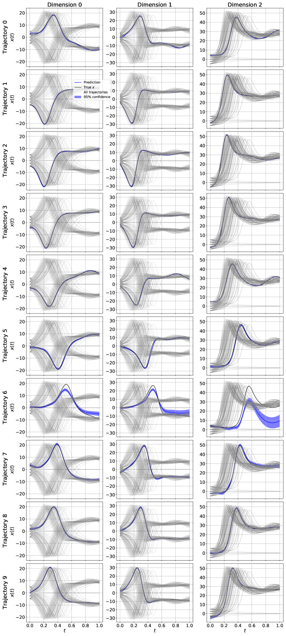
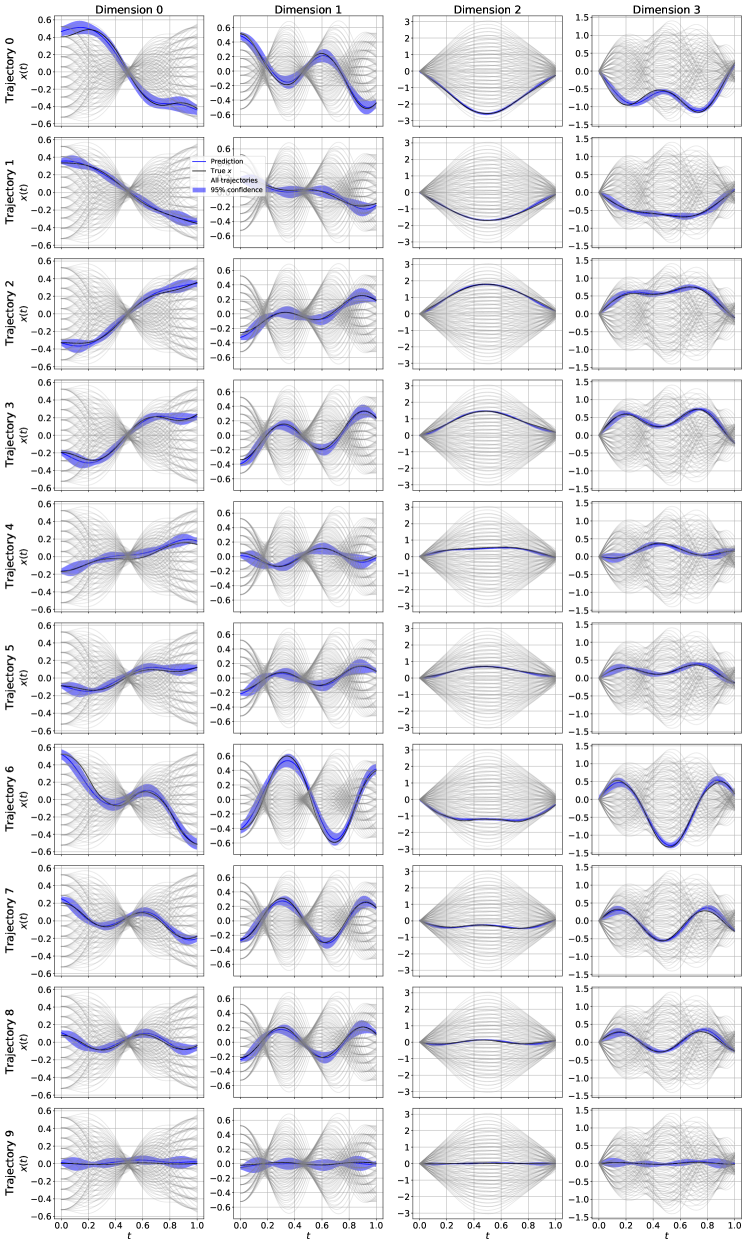
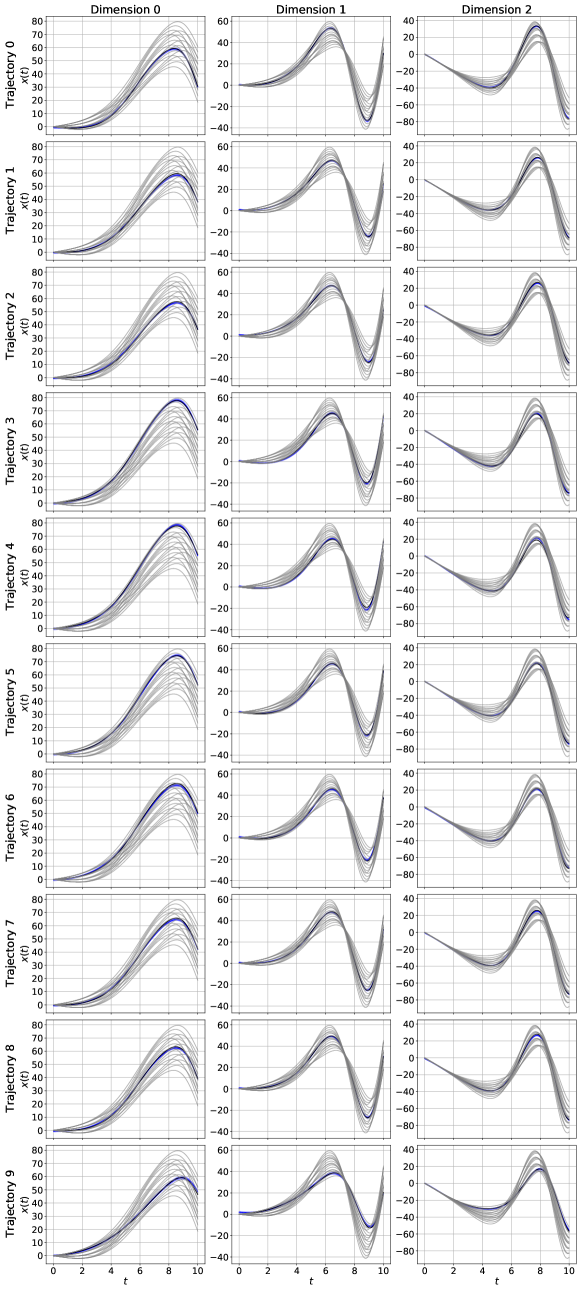
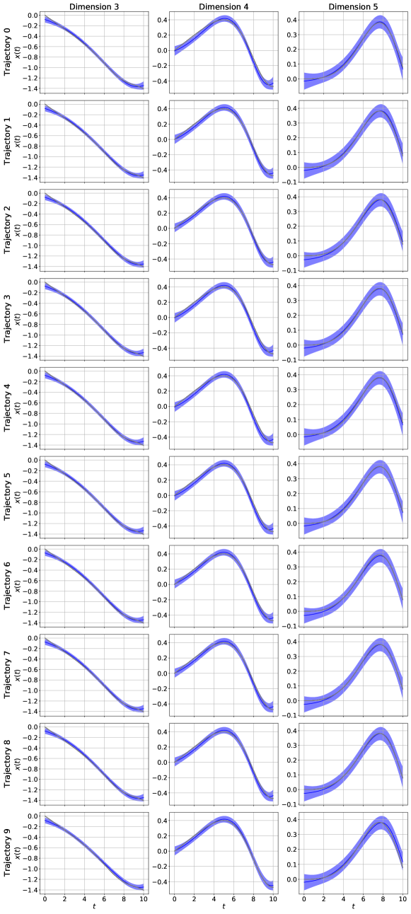
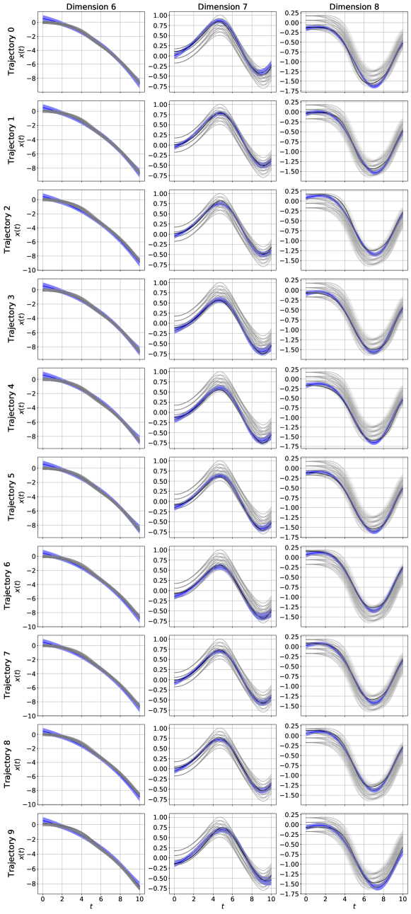
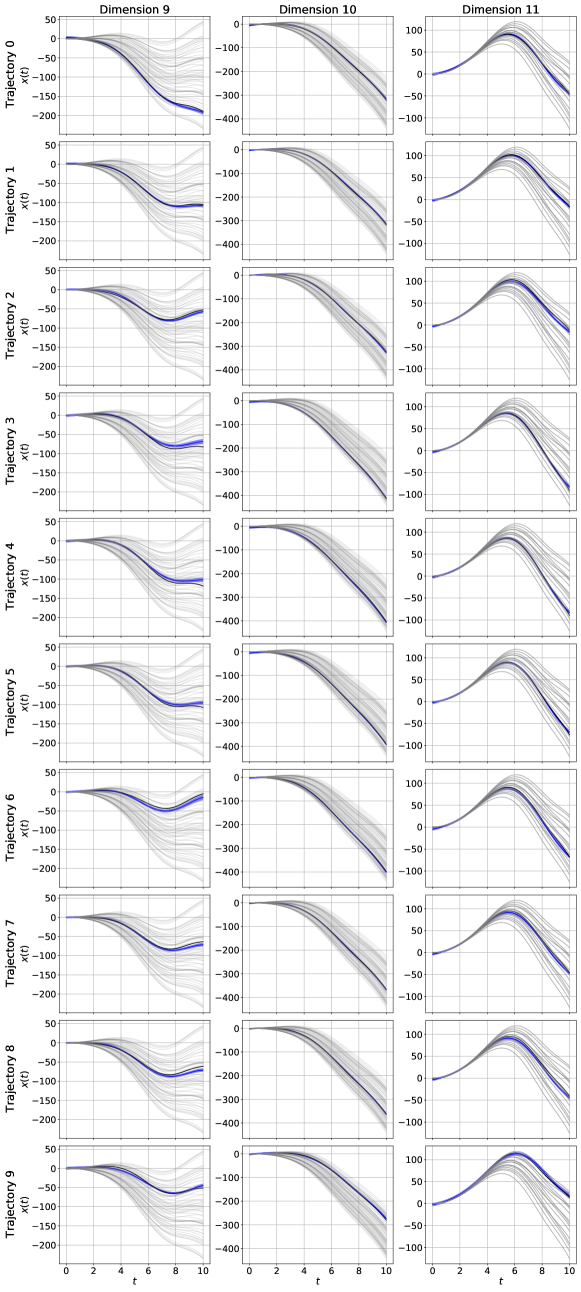
In this section, we first show the state predictions of $\operatorname{DGM}$ on the datasets with multiple trajectories. Then, we compare $\operatorname{DGM}$ with $\operatorname{SGLD}$ and $\operatorname{SGHMC}$ for the parametric case, i.e. where we assume to have access to the true parametric form of the dynamics. Since most datasets have too many trajectories to be fully visualized, we show a random subset instead.

E.1 Sample plots from trained trajectories

Figure 13: $\operatorname{DGM}$’s prediction on $5$ randomly sampled training trajectories of LV 100.

Figure 14: $\operatorname{DGM}$’s prediction on $8$ randomly sampled training trajectories of LO 125.

Figure 15: $\operatorname{DGM}$’s prediction on $10$ randomly sampled training trajectories of DP 100.

Figure 16: $\operatorname{DGM}$’s prediction on $10$ randomly sampled training trajectories of QU 64, for state dimensions $0$-$2$.

Figure 17: $\operatorname{DGM}$’s prediction on $10$ randomly sampled training trajectories of QU 64, for state dimensions $3$-$5$.

Figure 18: $\operatorname{DGM}$’s prediction on $10$ randomly sampled training trajectories of QU 64, for state dimensions $6$-$8$.

Figure 19: $\operatorname{DGM}$’s prediction on $10$ randomly sampled training trajectories of QU 64, for state dimensions $9$-$11$.

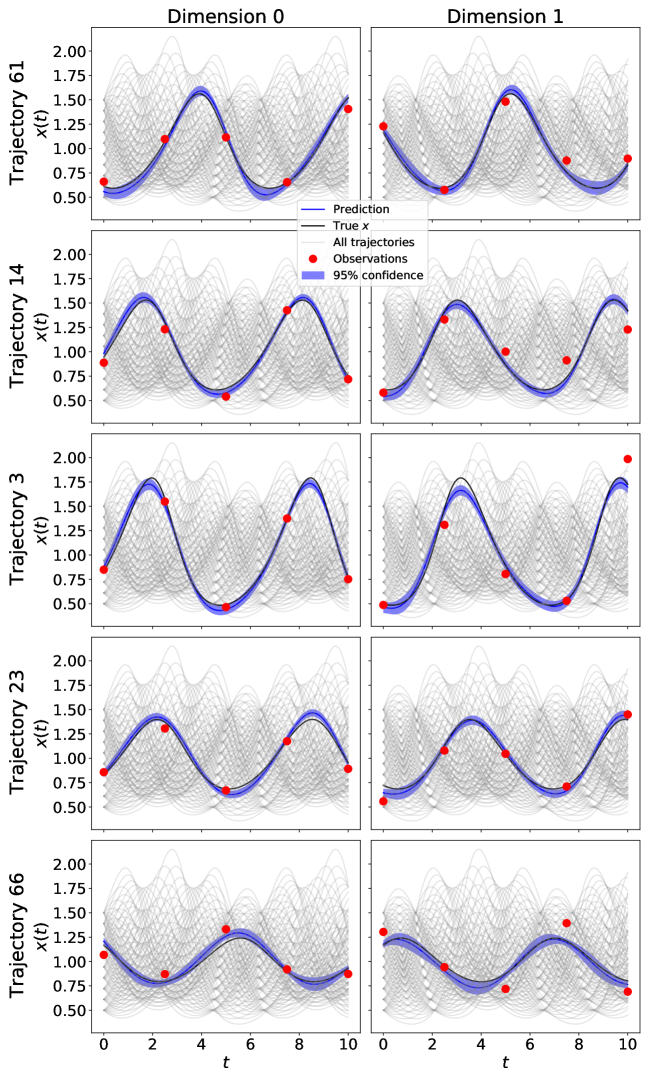
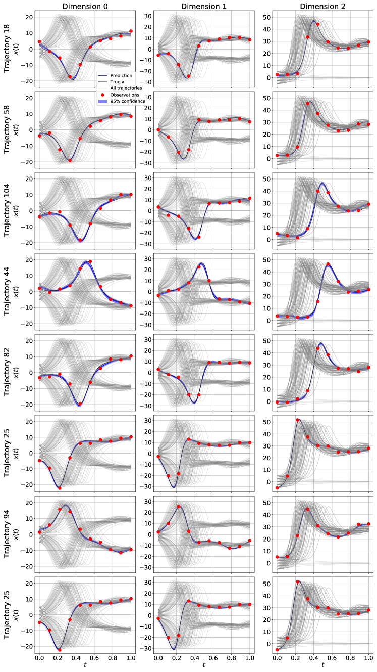
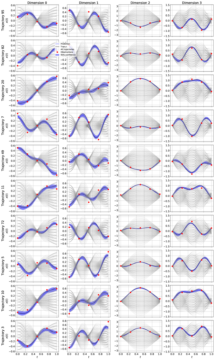
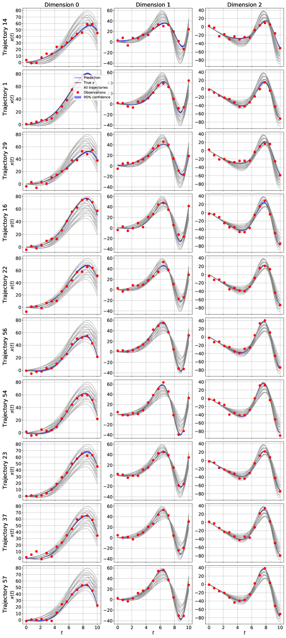
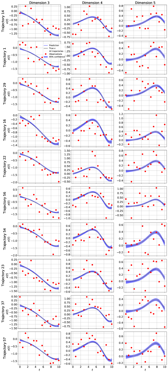
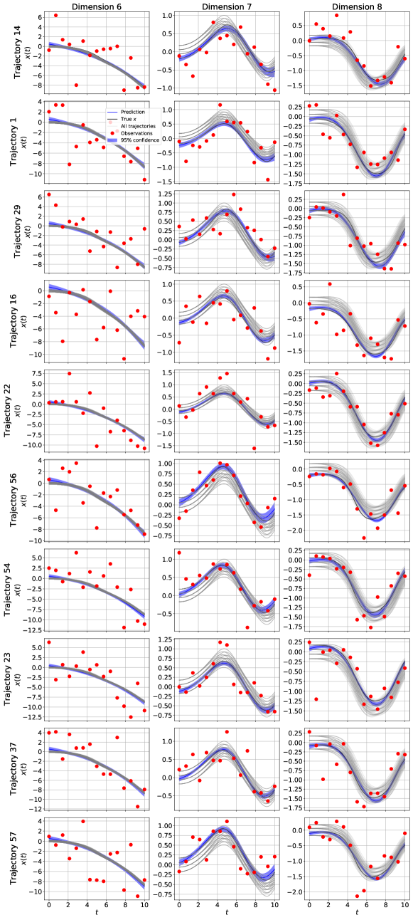
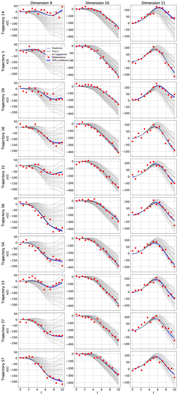
E.2 Sample plots from test trajectories

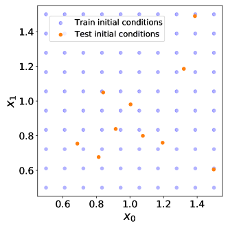
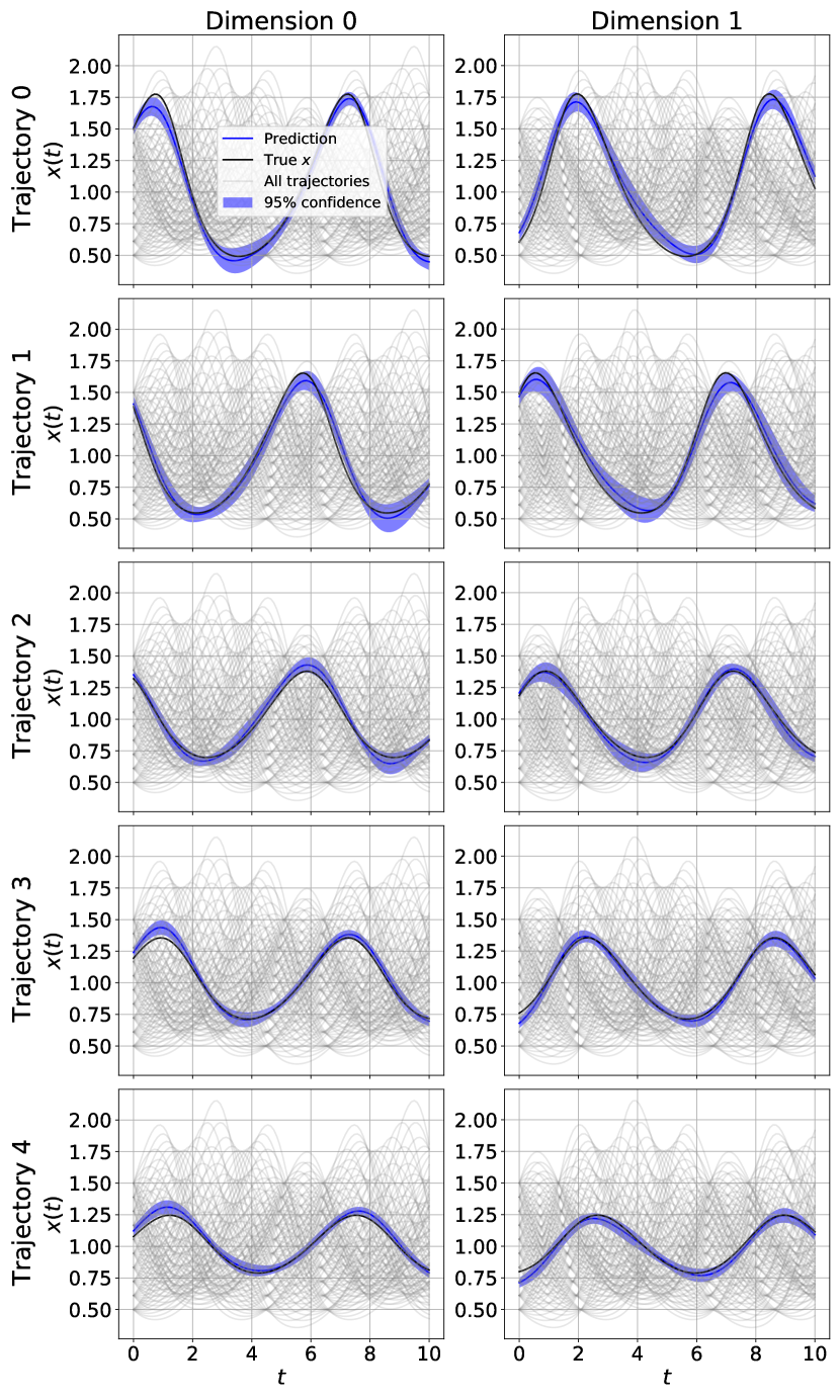
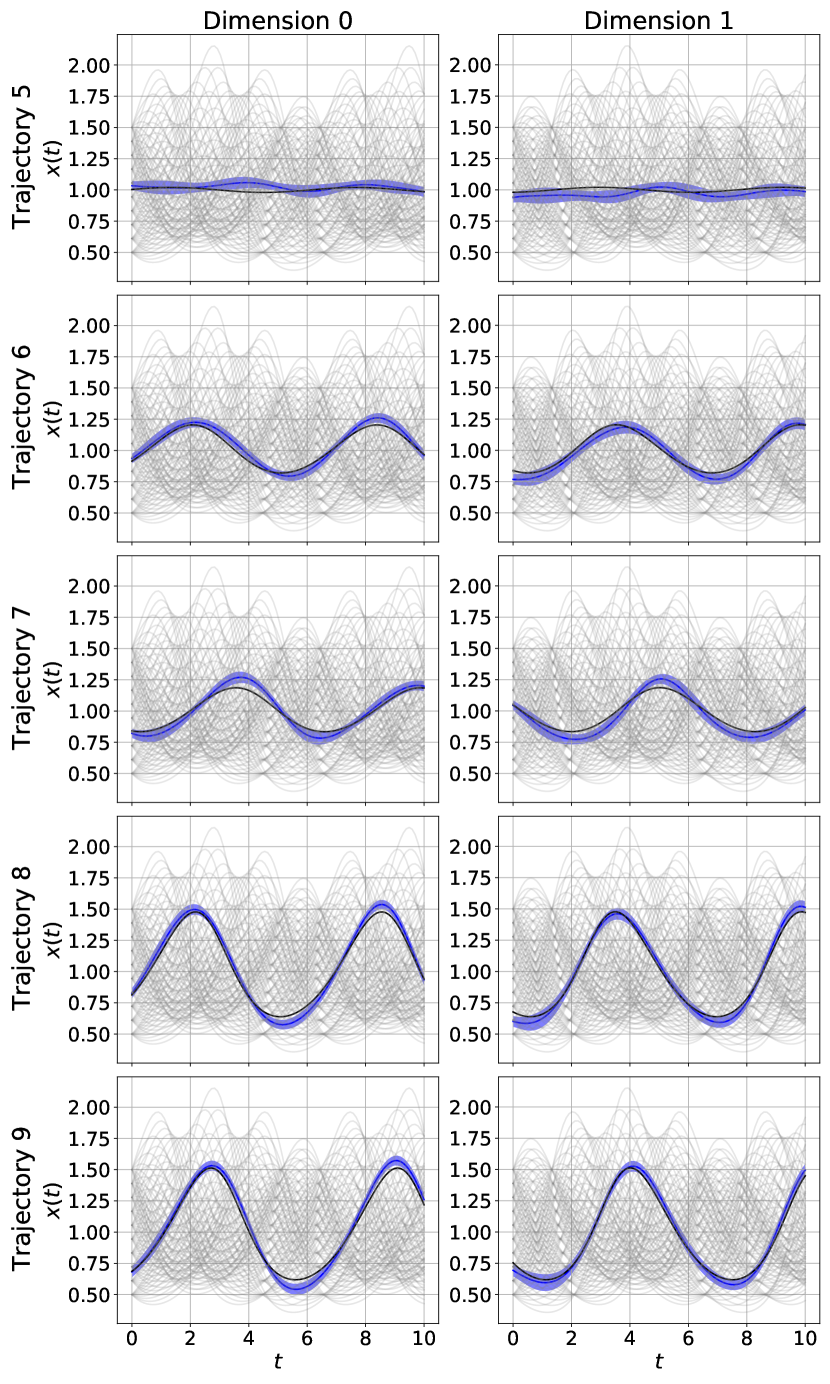
Here, we show $\operatorname{DGM}$’s predictions on the test trajectories used to test generalization, as introduced in Appendix A. Since LV 100 is a two dimensional system, we also show the placement of the train and test initial conditions in Figure 20.

Figure 20: Placement of the initial conditions for the train and test trajectories of the LV 100 dataset. We selected the initial conditions for the train trajectories by gridding $[0.5,1.5]^{2}$ with $10$ points in every dimension. We select initial conditions for test trajectories independently, uniformly at random from the cube $[0.5,1.5]^{2}$.

Figure 21: $\operatorname{DGM}$’s prediction on $10$ randomly sampled test trajectories for the LV 100 dataset.

Figure 22: $\operatorname{DGM}$’s prediction on $10$ randomly sampled test trajectories for the LO 125 dataset.

Figure 23: $\operatorname{DGM}$’s prediction on $10$ randomly sampled test trajectories for the DP 100 dataset.

Figure 24: $\operatorname{DGM}$’s prediction on $10$ randomly sampled test trajectories of QU 64, for state dimensions $0$-$2$.

Figure 25: $\operatorname{DGM}$’s prediction on $10$ randomly sampled test trajectories of QU 64, for state dimensions $3$-$5$.

Figure 26: $\operatorname{DGM}$’s prediction on $10$ randomly sampled test trajectories of QU 64, for state dimensions $6$-$8$.

Figure 27: $\operatorname{DGM}$’s prediction on $10$ randomly sampled test trajectories of QU 64, for state dimensions $9$-$11$.

E.3 Comparison with parameteric integration

In this subsection, we compare $\operatorname{DGM}$ against $\operatorname{SGLD}$ and $\operatorname{SGHMC}$ in the parametric setting, i.e. where we assume access to the parametric form of the true dynamics $\bm{f}(\bm{x},\bm{\theta})$. Despite serious tuning efforts outlined in Section C.2, we were unable to make $\operatorname{SGLD}$ and $\operatorname{SGHMC}$ perform on any multitrajectory experiments except for Lotka Volterra 100. As can be seen in Table 5, the sampling based methods seem to perform quite well. However, it should be noted that we were unable to get a stable performance without using ground truth information, as outlined in Section C.2. Given this caveat and the results of the non-parametric case in the main paper, we conclude the following. If strong and accurate expert knowledge is available that can be used to fix strong priors on simple systems, the sampling-based approaches are certainly a good choice. For more complex systems or in the absence of any expert knowledge, $\operatorname{DGM}$ seems to have a clear edge.

Table 5: Log likelihood of the ground truth of $100$ points on the training trajectories. $\operatorname{SGHMC}$ and $\operatorname{SGLD}$ were provided with strong, ground-truth-inspired priors and received an extensive hyperparameter sweep using the ground truth as metric. Nevertheless, $\operatorname{DGM}$ performs decently in comparison, without using neither priors nor ground truth.

	Log Likelihood
	$\operatorname{DGM}$	$\operatorname{SGLD}$	$\operatorname{SGHMC}$
LV 1	$1.98\pm 0.18$	$\mathbf{3.07\pm 0.685}$	$3.06\pm 0.517$
LO 1	$-0.52\pm 0.09$	$\mathbf{2.01\pm 0.548}$	F
DP 1	$2.16\pm 0.13$	$\mathbf{3.43\pm 0.396}$	$2.96\pm 0.795$
QU 1	$0.71\pm 0.07$	$\mathbf{2.42\pm 0.322}$	$1.38\pm 0.00$
LV 100	$1.85\pm 0.11$	$\mathbf{4.28\pm 0.184}$	$4.26\pm 0.178$

References

- Abbati et al., (2019) Abbati, G., Wenk, P., Osborne, M. A., Krause, A., Schölkopf, B., and Bauer, S. (2019). Ares and mars adversarial and mmd-minimizing regression for sdes. In International Conference on Machine Learning, pages 1–10. PMLR.
- Angelis et al., (2020) Angelis, E., Wenk, P., Schölkopf, B., Bauer, S., and Krause, A. (2020). Sleipnir: Deterministic and provably accurate feature expansion for gaussian process regression with derivatives. arXiv preprint arXiv:2003.02658.
- Berkenkamp et al., (2017) Berkenkamp, F., Turchetta, M., Schoellig, A., and Krause, A. (2017). Safe model-based reinforcement learning with stability guarantees. In Guyon, I., Luxburg, U. V., Bengio, S., Wallach, H., Fergus, R., Vishwanathan, S., and Garnett, R., editors, Advances in Neural Information Processing Systems, volume 30. Curran Associates, Inc.
- Bezanson et al., (2017) Bezanson, J., Edelman, A., Karpinski, S., and Shah, V. B. (2017). Julia: A fresh approach to numerical computing. SIAM Review, 59(1):65–98.
- Bishop, (2006) Bishop, C. M. (2006). Pattern Recognition and Machine Learning (Information Science and Statistics). Springer-Verlag, Berlin, Heidelberg.
- Bohlin, (2006) Bohlin, T. P. (2006). Practical grey-box process identification: theory and applications. Springer Science & Business Media.
- Bradbury et al., (2018) Bradbury, J., Frostig, R., Hawkins, P., Johnson, M. J., Leary, C., Maclaurin, D., Necula, G., Paszke, A., VanderPlas, J., Wanderman-Milne, S., and Zhang, Q. (2018). JAX: composable transformations of Python+NumPy programs.
- Brunton et al., (2016) Brunton, S. L., Proctor, J. L., and Kutz, J. N. (2016). Discovering governing equations from data by sparse identification of nonlinear dynamical systems. Proceedings of the national academy of sciences, 113(15):3932–3937.
- Calderhead et al., (2009) Calderhead, B., Girolami, M., and Lawrence, N. D. (2009). Accelerating bayesian inference over nonlinear differential equations with gaussian processes. In Advances in neural information processing systems, pages 217–224. Citeseer.
- Chen et al., (2018) Chen, R. T. Q., Rubanova, Y., Bettencourt, J., and Duvenaud, D. K. (2018). Neural ordinary differential equations. In Bengio, S., Wallach, H., Larochelle, H., Grauman, K., Cesa-Bianchi, N., and Garnett, R., editors, Advances in Neural Information Processing Systems, volume 31. Curran Associates, Inc.
- Chen et al., (2014) Chen, T., Fox, E., and Guestrin, C. (2014). Stochastic gradient hamiltonian monte carlo. In International conference on machine learning, pages 1683–1691. PMLR.
- Dandekar et al., (2021) Dandekar, R., Chung, K., Dixit, V., Tarek, M., Garcia-Valadez, A., Vemula, K. V., and Rackauckas, C. (2021). Bayesian neural ordinary differential equations. Symposium on Principles of Programming Languages, POPL.
- Deisenroth and Rasmussen, (2011) Deisenroth, M. and Rasmussen, C. E. (2011). Pilco: A model-based and data-efficient approach to policy search. In Proceedings of the 28th International Conference on machine learning (ICML-11), pages 465–472. Citeseer.
- Dondelinger et al., (2013) Dondelinger, F., Husmeier, D., Rogers, S., and Filippone, M. (2013). Ode parameter inference using adaptive gradient matching with gaussian processes. In Artificial intelligence and statistics, pages 216–228. PMLR.
- Fanfarillo et al., (2021) Fanfarillo, A., Roozitalab, B., Hu, W., and Cervone, G. (2021). Probabilistic forecasting using deep generative models. GeoInformatica, 25(1):127–147.
- Ghosh et al., (2021) Ghosh, S., Birrell, P., and De Angelis, D. (2021). Variational inference for nonlinear ordinary differential equations. In International Conference on Artificial Intelligence and Statistics, pages 2719–2727. PMLR.
- Gorbach et al., (2017) Gorbach, N. S., Bauer, S., and Buhmann, J. M. (2017). Scalable variational inference for dynamical systems. In Guyon, I., Luxburg, U. V., Bengio, S., Wallach, H., Fergus, R., Vishwanathan, S., and Garnett, R., editors, Advances in Neural Information Processing Systems, volume 30. Curran Associates, Inc.
- Greydanus et al., (2019) Greydanus, S., Dzamba, M., and Yosinski, J. (2019). Hamiltonian neural networks. In Wallach, H., Larochelle, H., Beygelzimer, A., d'Alché-Buc, F., Fox, E., and Garnett, R., editors, Advances in Neural Information Processing Systems, volume 32. Curran Associates, Inc.
- Hjalmarsson, (2005) Hjalmarsson, H. (2005). From experiment design to closed-loop control. Automatica, 41(3):393–438.
- Hoffman and Gelman, (2014) Hoffman, M. D. and Gelman, A. (2014). The no-u-turn sampler: adaptively setting path lengths in hamiltonian monte carlo. J. Mach. Learn. Res., 15(1):1593–1623.
- Houthooft et al., (2016) Houthooft, R., Chen, X., Chen, X., Duan, Y., Schulman, J., De Turck, F., and Abbeel, P. (2016). Vime: Variational information maximizing exploration. In Lee, D., Sugiyama, M., Luxburg, U., Guyon, I., and Garnett, R., editors, Advances in Neural Information Processing Systems, volume 29. Curran Associates, Inc.
- Ingalls, (2013) Ingalls, B. P. (2013). Mathematical modeling in systems biology: an introduction. MIT press.
- Jidling et al., (2017) Jidling, C., Wahlström, N., Wills, A., and Schön, T. B. (2017). Linearly constrained gaussian processes. In Guyon, I., Luxburg, U. V., Bengio, S., Wallach, H., Fergus, R., Vishwanathan, S., and Garnett, R., editors, Advances in Neural Information Processing Systems, volume 30. Curran Associates, Inc.
- Jones et al., (2009) Jones, D. S., Plank, M., and Sleeman, B. D. (2009). Differential equations and mathematical biology. CRC press.
- Kantorovich, (1939) Kantorovich, L. V. (1939). The mathematical method of production planning and organization. Management Science, 6(4):363–422.
- Karaman and Frazzoli, (2011) Karaman, S. and Frazzoli, E. (2011). Sampling-based algorithms for optimal motion planning. The international journal of robotics research, 30(7):846–894.
- Kelly et al., (2020) Kelly, J., Bettencourt, J., Johnson, M. J., and Duvenaud, D. K. (2020). Learning differential equations that are easy to solve. In Larochelle, H., Ranzato, M., Hadsell, R., Balcan, M. F., and Lin, H., editors, Advances in Neural Information Processing Systems, volume 33, pages 4370–4380. Curran Associates, Inc.
- Kersting et al., (2020) Kersting, H., Krämer, N., Schiegg, M., Daniel, C., Tiemann, M., and Hennig, P. (2020). Differentiable likelihoods for fast inversion of’likelihood-free’dynamical systems. In International Conference on Machine Learning, pages 5198–5208. PMLR.
- Kidger et al., (2020) Kidger, P., Chen, R. T., and Lyons, T. (2020). " hey, that’s not an ode": Faster ode adjoints with 12 lines of code. arXiv preprint arXiv:2009.09457.
- LaValle, (2006) LaValle, S. M. (2006). Planning algorithms. Cambridge university press.
- Liu et al., (2020) Liu, H., Ong, Y.-S., Shen, X., and Cai, J. (2020). When gaussian process meets big data: A review of scalable gps. IEEE transactions on neural networks and learning systems, 31(11):4405–4423.
- Ljung, (1998) Ljung, L. (1998). System Identification, pages 163–173. Birkhäuser Boston, Boston, MA.
- Ljung, (1999) Ljung, L. (1999). Model validation and model error modeling. Linköping University Electronic Press.
- Norcliffe et al., (2021) Norcliffe, A., Bodnar, C., Day, B., Moss, J., and Liò, P. (2021). Neural {ode} processes. In International Conference on Learning Representations.
- Ortega et al., (2018) Ortega, R., Praly, L., Aranovskiy, S., Yi, B., and Zhang, W. (2018). On dynamic regressor extension and mixing parameter estimators: Two luenberger observers interpretations. Automatica, 95:548–551.
- Ortega et al., (2002) Ortega, R., Van Der Schaft, A., Maschke, B., and Escobar, G. (2002). Interconnection and damping assignment passivity-based control of port-controlled hamiltonian systems. Automatica, 38(4):585–596.
- Pillonetto and De Nicolao, (2010) Pillonetto, G. and De Nicolao, G. (2010). A new kernel-based approach for linear system identification. Automatica, 46(1):81–93.
- Pillonetto et al., (2014) Pillonetto, G., Dinuzzo, F., Chen, T., De Nicolao, G., and Ljung, L. (2014). Kernel methods in system identification, machine learning and function estimation: A survey. Automatica, 50(3):657–682.
- Rackauckas et al., (2020) Rackauckas, C., Ma, Y., Martensen, J., Warner, C., Zubov, K., Supekar, R., Skinner, D., Ramadhan, A., and Edelman, A. (2020). Universal differential equations for scientific machine learning. arXiv preprint arXiv:2001.04385.
- Rahimi et al., (2007) Rahimi, A., Recht, B., et al. (2007). Random features for large-scale kernel machines. In NIPS, volume 3, page 5. Citeseer.
- Raissi et al., (2019) Raissi, M., Perdikaris, P., and Karniadakis, G. E. (2019). Physics-informed neural networks: A deep learning framework for solving forward and inverse problems involving nonlinear partial differential equations. Journal of Computational Physics, 378:686–707.
- Rasmussen, (2004) Rasmussen, C. E. (2004). Gaussian Processes in Machine Learning, pages 63–71. Springer Berlin Heidelberg, Berlin, Heidelberg.
- Schulman et al., (2015) Schulman, J., Levine, S., Abbeel, P., Jordan, M., and Moritz, P. (2015). Trust region policy optimization. In International conference on machine learning, pages 1889–1897. PMLR.
- Solak et al., (2003) Solak, E., Murray-Smith, R., Leithead, W. E., Leith, D. J., and Rasmussen, C. E. (2003). Derivative observations in gaussian process models of dynamic systems.
- Spong et al., (2006) Spong, M. W., Hutchinson, S., Vidyasagar, M., et al. (2006). Robot modeling and control, volume 3. wiley New York.
- Srinivas et al., (2010) Srinivas, N., Krause, A., Kakade, S., and Seeger, M. (2010). Gaussian process optimization in the bandit setting: no regret and experimental design. In Proceedings of the 27th International Conference on International Conference on Machine Learning, pages 1015–1022.
- Varah, (1982) Varah, J. M. (1982). A spline least squares method for numerical parameter estimation in differential equations. SIAM Journal on Scientific and Statistical Computing, 3(1):28–46.
- Welling and Teh, (2011) Welling, M. and Teh, Y. W. (2011). Bayesian learning via stochastic gradient langevin dynamics. In Proceedings of the 28th international conference on machine learning (ICML-11), pages 681–688. Citeseer.
- Wenk et al., (2020) Wenk, P., Abbati, G., Osborne, M. A., Schölkopf, B., Krause, A., and Bauer, S. (2020). Odin: Ode-informed regression for parameter and state inference in time-continuous dynamical systems. In Proceedings of the AAAI Conference on Artificial Intelligence, volume 34, pages 6364–6371.
- Wenk et al., (2019) Wenk, P., Gotovos, A., Bauer, S., Gorbach, N. S., Krause, A., and Buhmann, J. M. (2019). Fast gaussian process based gradient matching for parameter identification in systems of nonlinear odes. In The 22nd International Conference on Artificial Intelligence and Statistics, pages 1351–1360. PMLR.
- Wensing et al., (2017) Wensing, P. M., Kim, S., and Slotine, J.-J. E. (2017). Linear matrix inequalities for physically consistent inertial parameter identification: A statistical perspective on the mass distribution. IEEE Robotics and Automation Letters, 3(1):60–67.
- Wilson et al., (2016) Wilson, A. G., Hu, Z., Salakhutdinov, R., and Xing, E. P. (2016). Deep kernel learning. In Artificial intelligence and statistics, pages 370–378. PMLR.
- Wittenburg, (2013) Wittenburg, J. (2013). Dynamics of systems of rigid bodies, volume 33. Springer-Verlag.
- Xu et al., (2021) Xu, W., Chen, R. T., Li, X., and Duvenaud, D. (2021). Infinitely deep bayesian neural networks with stochastic differential equations. arXiv preprint arXiv:2102.06559.
- Yildiz et al., (2019) Yildiz, C., Heinonen, M., and Lähdesmäki, H. (2019). Ode2vae: Deep generative second order odes with bayesian neural networks. In Wallach, H., Larochelle, H., Beygelzimer, A., d'Alché-Buc, F., Fox, E., and Garnett, R., editors, Advances in Neural Information Processing Systems, volume 32. Curran Associates, Inc.
- Zhuang et al., (2020) Zhuang, J., Dvornek, N., Li, X., Tatikonda, S., Papademetris, X., and Duncan, J. (2020). Adaptive checkpoint adjoint method for gradient estimation in neural ode. In International Conference on Machine Learning, pages 11639–11649. PMLR.
- Zhuang et al., (2021) Zhuang, J., Dvornek, N. C., Tatikonda, S., and Duncan, J. S. (2021). Mali: A memory efficient and reverse accurate integrator for neural odes. arXiv preprint arXiv:2102.04668.
.tocmtappendix \etocsettagdepthmtchapternone \etocsettagdepthmtappendixsubsection