maars: Tidy Inference under the ‘Models as Approximations’ Framework in R
Abstract
Linear regression using ordinary least squares (OLS) is a critical part of every statistician’s toolkit. In R, this is elegantly implemented via lm() and its related functions. However, the statistical inference output from this suite of functions is based on the assumption that the model is well specified. This assumption is often unrealistic and at best satisfied approximately. In the statistics and econometrics literature, this has long been recognized and a large body of work provides inference for OLS under more practical assumptions. This can be seen as model-free inference. In this paper, we introduce our package maars (“models as approximations”) that aims at bringing research on model-free inference to R via a comprehensive workflow. The maars package differs from other packages that also implement variance estimation, such as sandwich, in three key ways. First, all functions in maars follow a consistent grammar and return output in tidy format, with minimal deviation from the typical lm() workflow. Second, maars contains several tools for inference including empirical, multiplier, residual bootstrap, and subsampling, for easy comparison. Third, maars is developed with pedagogy in mind. For this, most of its functions explicitly return the assumptions under which the output is valid. This key innovation makes maars useful in teaching inference under misspecification and also a powerful tool for applied researchers. We hope our default feature of explicitly presenting assumptions will become a de facto standard for most statistical modeling in R.††∗ Indicates equal contribution.
1 Introduction
Multiple linear regression is one of the most commonly used data analytic tools. Although the general notion of “all models are approximations” is well received in terms of inference under model misspecification, most statistical software (including R) does not yet have a comprehensive implementation of all such aspects. In detail, the elegant implementation of the ordinary least squares estimator through the lm() function is based on the classical and unrealistic assumptions of a linear model, i.e., linearity, homoscedasticity, and normality. The lm() implementation does provide methods for diagnosing these assumptions. However, it has long been recognized that inference should be performed under more general assumptions, even if the estimator is constructed based on likelihood principles (Huber, 1967; Buja et al., 2019a).
Over the years, several R packages such as car (Fox and Weisberg, 2019), clubSandwich (Pustejovsky, 2021), lmtest (Zeileis and Hothorn, 2002), and sandwich (Zeileis, 2004; Zeileis et al., 2020) have been developed to implement heteroscedasticity and non-linearity consistent estimators of the asymptotic variance. In this misspecified setting, a tidy workflow is currently unavailable in R. By a tidy workflow, we mean a suite of functions for variance estimation, confidence interval computation, hypothesis testing, and diagnostics that follow a consistent naming convention, whose outputs are tailored for further exploration, e.g., using the tidyverse set of packages (Wickham et al., 2019). In this paper, we introduce the maars package that provides such a tidy workflow for data analysis with ordinary least squares (OLS) linear regression. Our package is motivated, in large part, by the discussion of Buja et al. (2019a, b). Part of our motivation is also pedagogical, in making applied researchers more explicitly aware of the underlying assumptions and the consequences of model-based variance estimators for inference.
In this paper, we introduce the key functionality in the maars package. For illustrative purposes only, we use the LA Homeless data from Buja et al. (2019a) as a running example to demonstrate the maars package functionality.111The package is available at: https://github.com/shamindras/maars. As noted in Buja et al. (2019a), this dataset has observations, each representing a sampled metropolitan LA County Census tract. It also has numeric variables measuring different quantities of interest in each tract. For linear modeling purposes, the response variable (StreetTotal) is a count of the homeless people in each tract. There are six covariates for regression purposes. These include the Median Income of Households (MedianInc ($1000)), and the share of non-Caucasian residents (PercMinority). The remaining four covariates measure the proportion of the different types of lots in each tract (PercCommercial, PercVacant, PercResidential and PercIndustrial).
The rest of the paper is organized as follows. In Section 2, we detail the theoretical properties of the OLS estimator in both the well-specified and misspecified model settings. In Section 3, we describe the key design principles upon which maars is based. Section 4 and Section 5 focus on the variance estimation and graphical model diagnostic functionalities present in the package respectively. In Section 6, we give an overview of the pedagogical vignettes and and guided lesson-plans in the package. In Section 7, we discuss the open-source best practices that we adopted to help build an inclusive community for new users and contributors. Finally, in Section 8 we conclude by outlining future development plans.
2 Theoretical properties of OLS
2.1 OLS under well-specification
Suppose we have regression data . The well-specified (classical) linear model stipulates that are independent and satisfy
| (1) |
where . This implies that (linearity) and (homoscedasticity). Usually one also assumes covariates to be non-stochastic. Under these assumptions, we get that the OLS estimator
has a normal distribution (conditional on ):
| (2) |
This distribution yields confidence intervals, hypothesis tests, and -values for . The R function lm() provides inference based on (2). For the LA Homeless data, the implementation of OLS along with its inference (in Figure 1) are as follows:
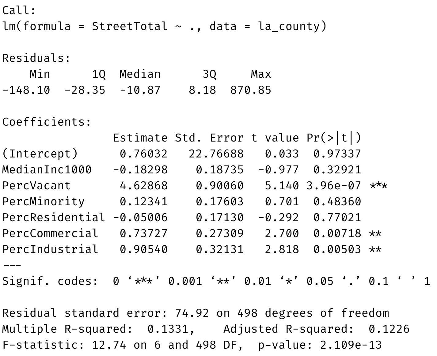
As mentioned, the standard errors, -scores, and the -values reported in the summary above are most likely invalid because the linear model for LA Homeless data is not well-specified (Buja et al., 2019a). We will now discuss the properties of OLS under misspecification of the linear model. It should be mentioned here that we will only discuss misspecification of the linear model but require independence of the observations. Dependence will be part of our future work (see Section 8).
2.2 OLS under misspecification
If are independent and identically distributed (i.i.d.), then the least squares estimator converges (in probability) to
| (3) |
where is an independent copy of and is the population projection parameter. If the linear model (1) holds true, then . Assuming only i.i.d. observations with finite moments, it is easy to obtain the normal limiting distribution:
| (4) |
where , and ; see Buja et al. (2019a) for details. A similar limit theorem also holds when the observations are independent but not identically distributed (i.n.i.d.).
The matrices and can be readily estimated by replacing the expectations by averages and by leading to the sandwich estimator ; see Kuchibhotla et al. (2018) for details. Here
| (5) |
It can be shown that consistently estimates the asymptotic variance under i.i.d. data and over-estimates the asymptotic variance under i.n.i.d. data (Kuchibhotla et al., 2018). It is noteworthy that the estimator converges to the model-based variance if the linear model (1) holds true. With a model-free estimator of the asymptotic variance, one can perform inference for using asymptotic normality. The asymptotic confidence interval for the coefficient is then given by
| (6) |
where is the quantile of the standard normal. The Wald test for linear restrictions of the coefficients of the form , where and are a matrix and a dimensional vector respectively, is still valid under only the assumption of independence. Under the null hypothesis, the Wald test statistic asymptotically follows a distribution with degrees of freedom; see, e.g., White (1982, Theorem 3.4).
3 maars: Designed for research and pedagogy
Our goal is for the maars package to be a natural research workflow for model-free OLS inference in R. Equally importantly, we also intend for maars to be a useful pedagogical tool to help convey these rich inferential concepts. In order to satisfy this dual research and pedagogical purpose, maars is built according to the following five design principles (DP.1–DP.5):
-
DP.1
Build a flexible API to enable easy user access to a diverse set of inferential tools.
-
DP.2
Ensure that the assumptions for all modeling techniques explicit to the user.
-
DP.3
Develop a consistent tidy grammar for OLS inference under model misspecification to enhance communication of code with other users and developers.
-
DP.4
Emphasize teaching these inferential techniques and concepts through instructive examples.
-
DP.5
Utilize modern open-source best practices to create an inclusive package development environment.
We provide brief details on the design principles DP.1–DP.5 and details of how they are applied in maars. First, by DP.1, we intend for maars to provide a user-friendly way to access the rich set of OLS inferential techniques under model misspecification. This is primarily achieved through the comp_var() function, which provides a common API for the user for OLS modeling purposes. By DP.2 we want to ensure that the assumptions behind the modeling techniques are made explicit to the user. By DP.3 we have adopted in maars a consistent function naming convention that follows a tidy grammar and where tidy tibble outputs are returned whenever feasible. This is to better facilitate downstream analysis and communication of results. Details of DP.1–DP.3 are emphasized with examples in Sections 4 and 5.
In DP.4 we emphasize the use of detailed instructive vignettes to teach the inferential techniques for OLS using a tidy maars workflow. See Section 6 for more details. Finally, in DP.5 our aim is for maars to be a long-term part of a applied researcher’s OLS toolkit in R. We achieve this by following and adapting to the best open-source package development practices, and thus building an inclusive environment around maars. For example, we ensure that the maars functions are rigorously benchmarked and unit tested. A well defined benchmarking framework demonstrates how our code is optimized for computational efficiency. A detailed unit testing framework allows us to effectively perform statistical validation and error handling. See Section 7 for details. Finally, we note that the maars package is developed in an open-source manner that is inclusive towards new users and contributors.
4 Variance estimation and inference in maars
Under model misspecification, one of the main inferential tools is accurate and efficient estimation of variance. The maars modeling framework offers a variety of OLS inferential tools that are readily usable as part of a tidy pipe-friendly (%>%) workflow (Bache and Wickham, 2020).
These tools fall into three categories. First, we have closed-form variance estimators that are computed by default, i.e., lm() and the sandwich standard errors. Second, we have resampling-based variance estimators. These include the empirical bootstrap, multiplier bootstrap, residual bootstrap, and the subsampling-based methods. Third, we provide by default valid hypothesis testing under OLS model misspecification via tests. The workhorse that enables the simultaneous computations of the several types of variance estimates is the comp_var() function, which provides a common API for the user to access these estimators. For the sake of brevity, in Section 4.1 and Section 4.2 we show how the variance estimators can be run by the user, without displaying individual code outputs. In Section 4.3 we present how the consolidated output summary of all computed variance estimators can be used for downstream inference. We now review the functionality behind each estimation method in turn in this section, starting with the closed-form variance estimators.
4.1 Closed-form variance estimation
In maars, we provide two closed form variance estimators: one based on the assumption of a well-specified linear model and another based on the asymptotic normality under potential misspecification of the linear model.
Under the “models as approximations” framework, using only the independence of observations and finite moment assumptions, the asymptotic variance of the OLS estimates can be estimated by the sandwich estimator (Buja et al., 2019a, b): with and defined in (5). Then the standard error for the coefficient is given by . The classical estimator of asymptotic variance under a well-specified linear model is , for the residual sum of squares based estimator . In the maars package, this and other inferential summary statistics can be readily computed by calling the comp_var() function as follows.
The sandwich estimator is always computed by default, even when no arguments are passed in comp_var(). In the above code, maars_var_sand is an object of class maars_lm. This new object represents an modified version of the mod_fit object of class lm augmented with the newly computed sandwich variance estimates. As a result, comp_var() also returns by default the well-specified OLS standard error output.
4.2 Resampling-based variance estimation
In this subsection, we discuss the resampling-based variance estimation tools in maars. These resampling-based variance estimators are not computed by default in comp_var() and instead require a list of parameter inputs to be passed in by the user. We now describe the details each of the methods in turn.
4.2.1 Empirical bootstrap
Under the independence and finite moment assumptions, another method for the estimation of variance is the empirical bootstrap. The -out-of- empirical bootstrap consists of two steps. In the first step, for , we resample with replacement observations from the original data set and obtain the OLS estimate on the bootstrapped data set. In the second step, we compute times the sample covariance of as an estimate of , the asymptotic variance of . The justification for this method follows from the fact that, conditional on the original data , we have
| (7) |
and thus we can show that
| (8) |
Here . Therefore, as increases, the covariance of the OLS estimates on the bootstrapped data sets converges in probability to . We refer the reader to Bickel et al. (1997) for more details. In maars, the -out-of- empirical bootstrap estimates for the LA Homeless data can be obtained as follows. In this dataset, there are observations and hence setting is the same as running the -out-of- empirical bootstrap.
4.2.2 Multiplier bootstrap
The main disadvantage of the empirical bootstrap is that it requires the computation of the OLS estimate times. Furthermore, the bootstrapped design matrix might be singular. The multiplier bootstrap is an alternative method that helps overcome these difficulties. The method consists of estimating times
| (9) |
The weights are independent with and , for each , . These can be computed as follows:
The distribution of the weights in (9) is specified through the weights_type parameter. Following the boottest package (Roodman et al., 2019) in Stata, we provide the user with four prespecified options: rademacher, mammen, webb, gaussian. The rademacher weights are sampled from the two point Rademacher distribution which has takes values , with equal probability. The mammen weights are sampled from the two point Mammen distribution which takes values , with probabilities , respectively. The webb weights are sampled from the six point Webb distribution which takes values , with equal probability. Finally, the gaussian weights are sampled from the standard Gaussian distribution.
4.2.3 Residual bootstrap
One of the classical resampling methods for linear regression is residual bootstrap. In this method, one resamples the residuals instead of the pairs as in empirical bootstrap. With representing the OLS estimator, let the residuals be denoted by . Residual bootstrap consists of estimating times
| (10) |
where for are drawn i.i.d. from the empirical distribution of . From the closed form expression of , it readily follows that conditionally on the original data , as , where . This convergence in distribution does not require any of the linear model assumptions. However, the asymptotic variance of the residual bootstrap estimator matches the linear model based closed-form variance estimator and is not valid under model misspecification. In maars, residual bootstrap variance estimator can be obtained as follows:
4.2.4 Subsampling
An alternative to bootstrap is subsampling (Politis and Romano, 1994). Given our discussion on empirical (-out-of-) bootstrap, subsampling can be described as the -out-of- bootstrap where samples are drawn without replacement from the original data. Recall that the -out-of- bootstrap draws samples with replacement. Unlike the -out-of- bootstrap where can be of the same order as or even larger, subsampling validity usually requires . We refer the reader to Politis and Romano (1994) for details. Subsampling is more generally applicable than empirical and multiplier bootstrap schemes, allowing for valid inference even with stationary dependent data. In maars, subsampling can be run as follows:
4.3 Putting it all together: Summarizing the results
In Section 4.1 and Section 4.2, we have demonstrated how the maars package can be used to compute the variance of the coefficients estimates based on the sandwich estimator, the bootstraps, and subsampling. Although we have presented the code for each of the methods separately for instructive purposes, all of these variance estimators can be computed simultaneously through a single call of the comp_var() function as follows:
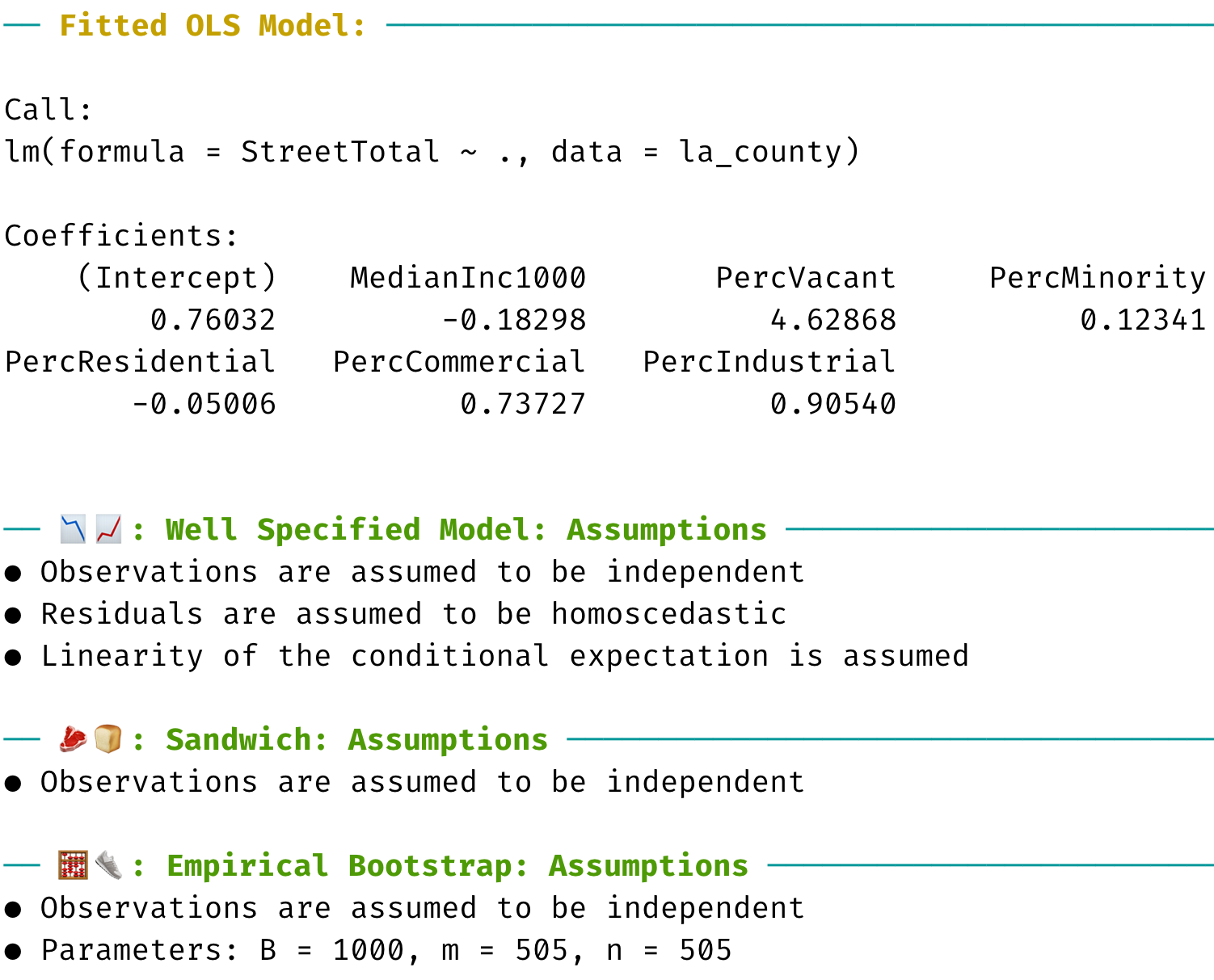
The maars_var object (i.e., of class maars_lm) by default supports the generic print() and summary() methods in R that are typically called on lm() objects, for instance. In fact, for our newly created maars_var object, a natural first step in the maars inferential workflow is for the user to simply run the generic print() method. This can be used to generate a summary of the OLS estimates and of the assumptions behind each of the variance estimation methods that have been employed:
As shown in the left panel of Figure 2, this method essentially returns an augmented version of the typical print() called on an lm object. Besides the OLS estimates, for each variance estimation methods that has been used in comp_var(), the assumptions (e.g., homoscedasticity) and parameters chosen (e.g., , , and ) are displayed. We hope our default feature of explicitly presenting assumptions will become a de facto standard for most statistical modeling in R.
The computed inferential statistics can be obtained as follows:
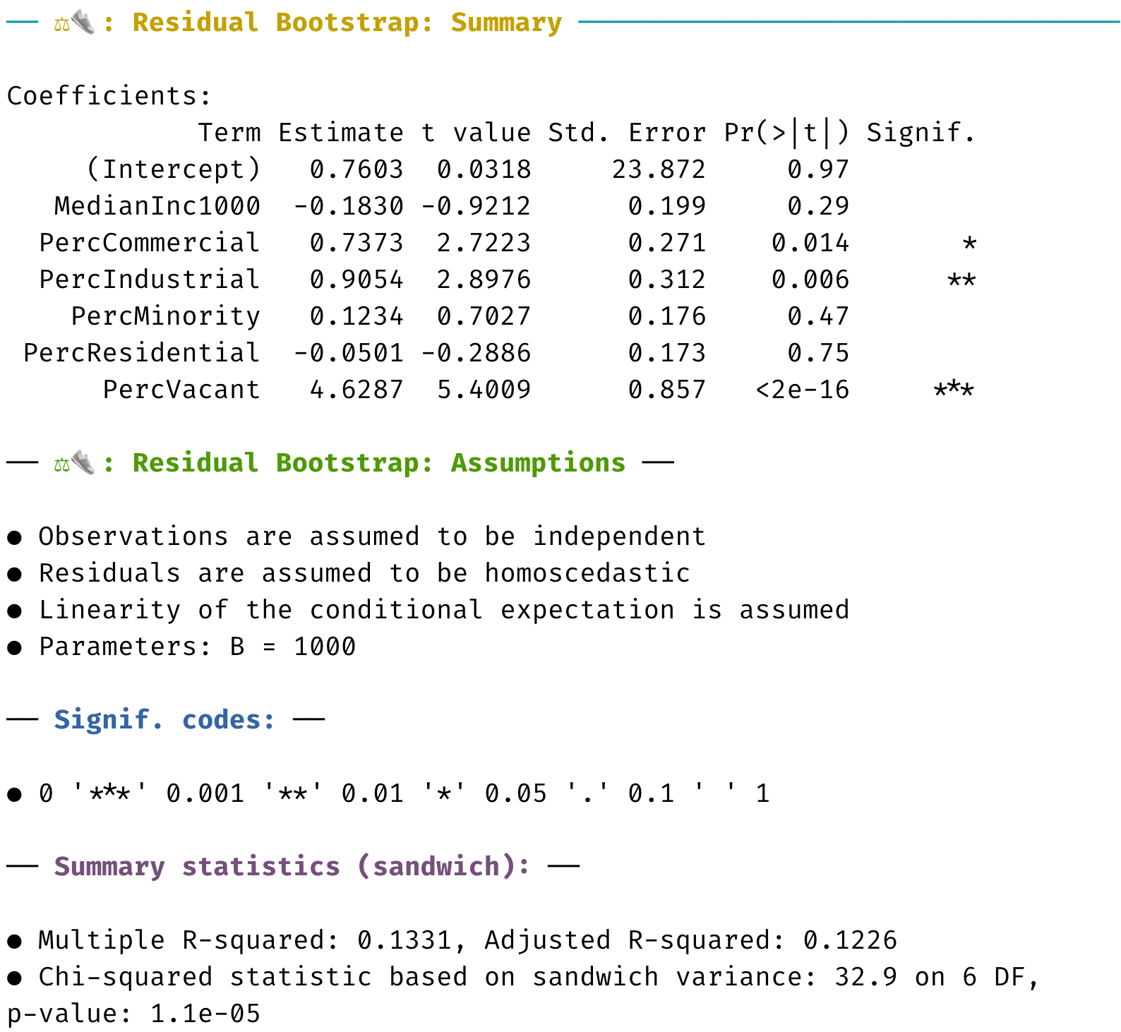
As shown in the right panel of Figure 2, calling the summary() method on a maars_lm object prints a stacked series of tibbles in a similar format as returned by the tidy() function in the broom package (Robinson et al., 2020). They are based on the different variance estimation methods, together with the related sets of assumptions. The result of a test for testing the null hypothesis that the OLS coefficients are all equal to 0 is reported at the bottom of the printed output. We make use of the cli package (Csárdi, 2021) to produce well-structured console output for both the print() and summary() methods.
In order to simplify downstream manipulation of the results, the generic methods present in maars have tidy analogues. For example, the user can obtain the set of OLS estimates and variance estimates in the form of a tibble by running get_summary(maars_var). More specifically, these functions begin with a consistent get_ prefix and return tidy tibble objects for data, ggplot2 objects for plots. By tidy tibble output we mean data in which every column is a variable, every row is an observation, and every cell is a single value (Wickham, 2014). We believe that this tidy grammar for function naming enables efficient further analysis of results using the tidyverse or similar R packages.
5 Visual diagnostic tools
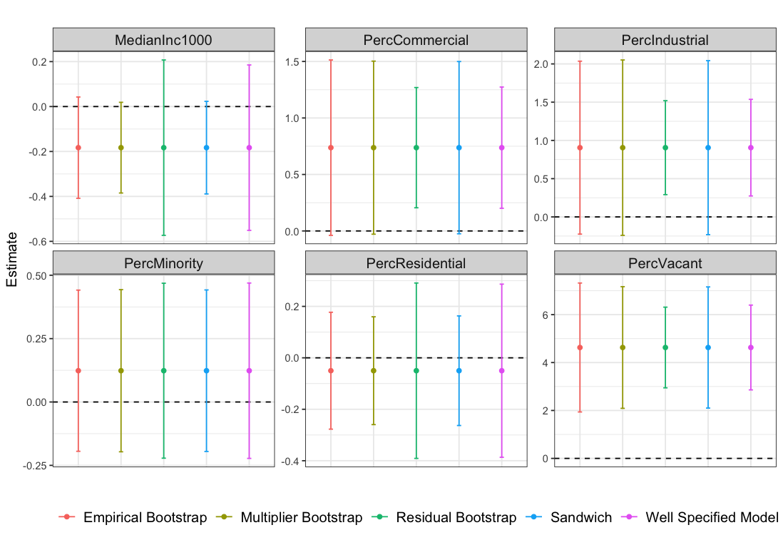
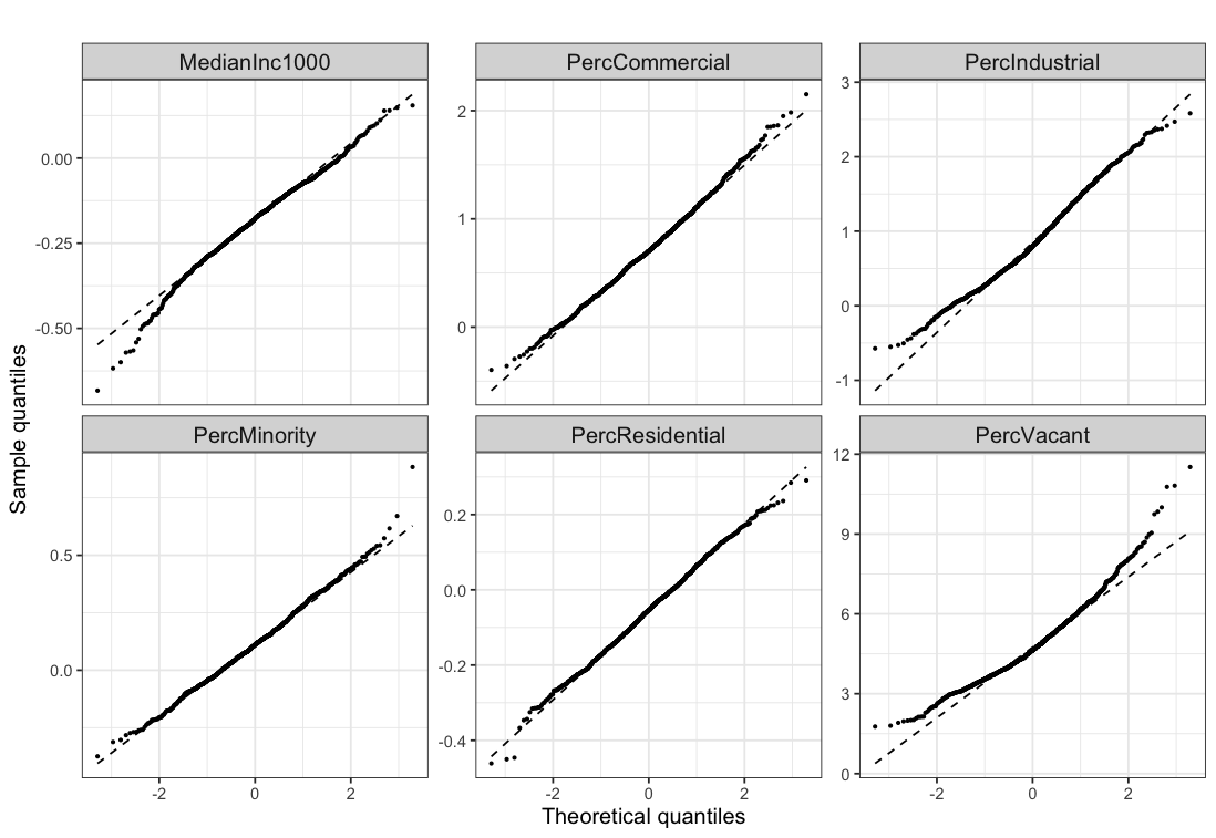
Using the maars_var object that we created in Section 4, the user can readily inspect the model’s fit via model diagnostic plots by calling the plot() method and its related tidy analogue get_plot(). These functions return eight graphical diagnostics. Six of them correspond to the same output that is generated by calling plot(mod_fit). These are the same plots returned from the classical lm() object but returned as ggplot2 objects. The two additional diagnostics are presented in Figure 3. The diagnostic in the left panel displays the widths of the different 95% confidence intervals for the OLS coefficients estimates. This graphical tool allows the user to visually compare the variance estimators computed using comp_var. Recall that the lm() and the residual bootstrap based variance estimator are only valid under a well-specified linear model, whereas the empirical, multiplier bootstrap, and subsampling variance estimator are model-free. Therefore, the visual comparison of estimated variances (as in the left panel of Figure (3)) already provides evidence of misspecification, if any. The last diagnostic, which is shown in the right panel of Figure 3, presents the distribution of the OLS estimates on the bootstrapped data sets. Through this tool, the user can compare the distribution of the estimates via a normal Q-Q plot to visually check whether sample size is large enough to justify the asymptotic regime.
The maars package also includes the three graphical diagnostic tools proposed in Buja et al. (2019b). When the regression model is correctly specified, the regression coefficients do not depend on the distribution of ; see Buja et al. (2019b, Proposition 4). Equivalently, variations in the OLS estimates under reweighting of would suggest that the model is not well-specified. In maars, we have implemented the graphical model diagnostics tools through which one can investigate whether the OLS assumptions are broken. These tools, which were proposed by Buja et al. (2019b), supplement of the model diagnostics returned by lm().
The key idea behind these model diagnostics is to study how the OLS estimates vary under arbitrary reweighting of . It is hard visualize such a diagnostic with arbitrary reweighting and hence we restrict to reweighting along certain regressors, as in Buja et al. (2019b). Although restrictive, the resulting plots provide intuitive understanding of misspecification in data. For reweighting along the -th regressor , , we do the following two operations:
-
DT.1
Select a grid of values (or centers) on the support of .
-
DT.2
For each center , compute the weighted least squares estimator
(11) Intuitively, this is the least squares estimator that gives more weight to observations that have -th regressor values close to .
The procedure consists of fitting regressions. This will give us one curve and for comparison, we also run the same procedure on bootstrapped data leading to . The tibble containing the OLS estimates based on the reweighting procedure can be obtained using the following function:
In the package, we have developed two types of grids for DT.1. The default grid of reweighting centers in DT.1 is based on the deciles of as in Buja et al. (2019b). Alternatively, the user can select a grid of evenly spaced values between and . For DT.2, maars uses . To assist the data scientist in interpreting the results of the refitting procedure, Buja et al. (2019b) have proposed using the following three graphical model diagnostics tools.
-
•
focal slope: Consider changes in coefficient of interest to the reweighting of each of the regressors , ; this provides insights into the interactions between regressor and all other regressors .
-
•
nonlinearity detection: Consider changes in to the reweighting of its own regressor ; this provides insights into marginal nonlinear behaviors of the response surface.
-
•
focal reweighting variable: Consider changes in all coefficients to the reweighting of a given regressor .
For further information and interpretations of these types of diagnostics, see Buja et al. (2019b, Section 5). The three types of graphical diagnostics can be obtained in maars as follows.
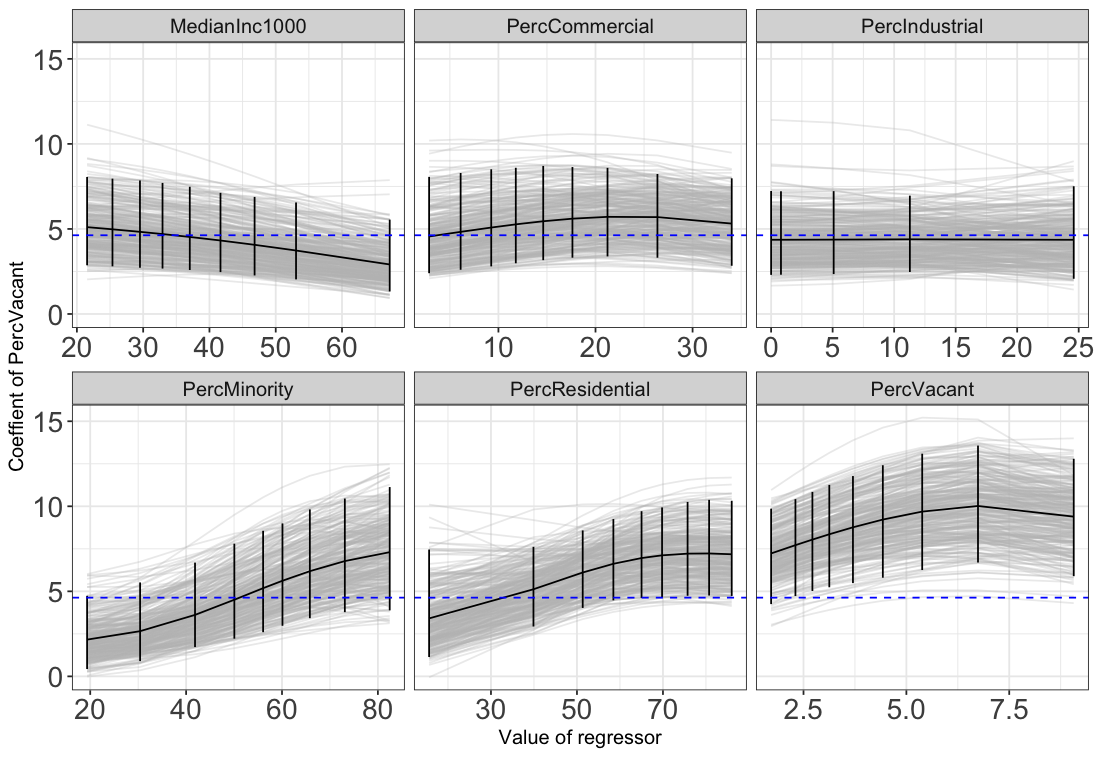
A sample output of the focal slope diagnostics is shown in Figure 4. These plots show how the OLS estimate of the prevalence of vacant lots (PercVacant) in our running example for 300 bootstrapped data sets (gray lines) vary under reweighting of all regressors (plot panel titles). The changes observed in the means of the estimates (black lines in the middle of each panel) indicate that the model is unlikely to be well-specified. In particular, these plots suggest the presence of an interaction between PercVacant and other regressors such as PercMinority, PercResidential, and MedianInc ($1000). In the plot in the bottom right corner, which depicts the estimate of PercVacant under reweighting of its own regressor, we observe that the reweighted estimates are far larger than the unweighted ones on the original data (blue dashed line).
6 Teaching by example: vignettes
As previously noted, maars is developed as a pedagogical (and research) tool to convey the rich techniques and concepts for OLS under model misspecification. Specifically, per DP.4 we emphasize teaching these concepts through guided case studies using tidy maars workflows. Our goal is to showcase these case studies as vignettes on our official package website.
These vignettes take two main forms. First, we take the core research papers upon which maars is based and reproduce tables and plots from them (Buja et al., 2019a, b). The intent here is to make the latest theoretical research in OLS under model misspecification accessible to the data scientist in a hands-on manner. Second, we provide lesson plan vignettes for these inferential techniques. For example, we know that both empirical and multiplier bootstrap are valid under model misspecification, but how different are they in practice? A systematic way to approach this question in a classroom setting (and beyond) is to observe that they contain the number of bootstrap replications, , as a common parameter. Under a simulated misspecified linear model, we demonstrate using a tidy maars workflow how to plot the confidence interval coverage, and average confidence width for these two estimators, as a function of the common parameter . The tidy maars grammar helps illustrate how to efficiently and consistently prototype these concepts in R, particularly to new students. We currently have two such case studies available and plan to extend this to a much a larger repository of research and pedagogical vignettes in the near future.
7 Open-source best practices
Our goal in developing the maars package is for it to be a standard R workflow for OLS inference under the model misspecification framework described in Buja et al. (2019a, b), and related literature. Per DP.5, we have strived to implement and adapt to open-source best practices to ensure an inclusive community for all users and contributors.
In developing the maars package, we have setup benchmarking using the bench package (Hester, 2020). We plan to conduct high-precision benchmarking of the core maars package functionality, and to assist in future code efficiency profiling efforts. Similarly, we currently test our statistical functionality and error handling using the testthat package (Wickham, 2011). Moreover, testing is built into the development cycle through cross-platform continuous integration using Github Actions. We use the tidyverse contributing guide and code of conduct to ensure that new contributors have ample guidance on the maars package development practices.
8 Conclusion and future work
In this paper, we introduce the maars package functionality to perform OLS inference under model misspecification. The maars package is designed to implement the key inferential ideas from Buja et al. (2019a, b) in a tidy R workflow.
The maars package is built on five core software design principles (see DP.1–DP.5). These design principles affect the day-to-day model-free inferential workflow. They also influence the way in which users can contribute to the existing maars functionality. The main tools for statistical inference in this framework are based on different variance estimation methods. These variance estimation tools in maars include closed-form variance estimators and standard errors computed using resampling techniques. By default maars provides valid hypothesis testing under model misspecification, i.e., reporting tests rather than tests. To help diagnose issues under the misspecified setting, there are a number of visualization tools readily accessible to maars user. These currently include the focal slope graphs of regressor variables (Buja et al., 2019b) and the Q-Q plots.
The maars package is still in active development and the final version we envision includes more tools related to misspecification. Implementation of analysis of variance (ANOVA) under misspecification and conformal inference based prediction (Vovk et al., 2005, Section 2.3) is in testing phase and will be added to the package soon. Further future work includes other variants of inference under dependent and time series data (beyond subsampling) as well as cluster robust standard errors. Finally, we want to extend the functions to GLMs, the Cox proportional hazards model, and inference after data exploration, e.g., PoSI (Kuchibhotla et al., 2020). We intend to demonstrate new package functionalities through more illustrative case study vignettes.
Acknowledgements
The authors would like to thank the members of the Larry’s group at the Wharton Statistics Department for their valuable feedback and encouragement during this work (listed alphabetically by surname): Richard Berk, Andreas Buja, Junhui Cai, Edward George, Elizabeth Ogburn, and Linda Zhao. The authors would also like to thank Alex Reinhart from the CMU Department of Statistics & Data Science for sharing valuable insights which informed our package development.
References
- Bache and Wickham [2020] Stefan Milton Bache and Hadley Wickham. magrittr: A Forward-Pipe Operator for R, 2020. URL https://CRAN.R-project.org/package=magrittr. R package version 2.0.1.
- Bickel et al. [1997] PJ Bickel, F Gotze, and WR van Zwet. Resampling fewer than n observations: gains, losses, and remedies for losses. Statistica Sinica, 7:1–31, 1997.
- Buja et al. [2019a] Andreas Buja, Lawrence Brown, Richard Berk, Edward George, Emil Pitkin, Mikhail Traskin, Kai Zhang, and Linda Zhao. Models as approximations I: consequences illustrated with linear regression. Statist. Sci., 34(4):523–544, 2019a. ISSN 0883-4237.
- Buja et al. [2019b] Andreas Buja, Lawrence Brown, Arun Kumar Kuchibhotla, Richard Berk, Edward George, and Linda Zhao. Models as approximations II: A model-free theory of parametric regression. Statist. Sci., 34(4):545–565, 2019b. ISSN 0883-4237.
- Csárdi [2021] Gábor Csárdi. cli: Helpers for Developing Command Line Interfaces, 2021. URL https://CRAN.R-project.org/package=cli. R package version 2.4.0.
- Fox and Weisberg [2019] John Fox and Sanford Weisberg. An R Companion to Applied Regression. Sage, Thousand Oaks CA, third edition, 2019.
- Hester [2020] Jim Hester. bench: High Precision Timing of R Expressions, 2020. URL https://CRAN.R-project.org/package=bench. R package version 1.1.1.
- Huber [1967] Peter J Huber. The behavior of maximum likelihood estimates under nonstandard conditions. In Proceedings of the fifth Berkeley symposium on mathematical statistics and probability, volume 1, pages 221–233. University of California Press, 1967.
- Kuchibhotla et al. [2018] Arun K Kuchibhotla, Lawrence D Brown, and Andreas Buja. Model-free study of ordinary least squares linear regression. arXiv preprint arXiv:1809.10538, 2018.
- Kuchibhotla et al. [2020] Arun K. Kuchibhotla, Lawrence D. Brown, Andreas Buja, Junhui Cai, Edward I. George, and Linda H. Zhao. Valid post-selection inference in model-free linear regression. Ann. Statist., 48(5):2953–2981, 2020. ISSN 0090-5364.
- Politis and Romano [1994] Dimitris N Politis and Joseph P Romano. Large sample confidence regions based on subsamples under minimal assumptions. The Annals of Statistics, pages 2031–2050, 1994.
- Pustejovsky [2021] James Pustejovsky. clubSandwich: Cluster-Robust (Sandwich) Variance Estimators with Small-Sample Corrections, 2021. URL https://CRAN.R-project.org/package=clubSandwich. R package version 0.5.3.
- Robinson et al. [2020] David Robinson, Alex Hayes, and Simon Couch. broom: Convert Statistical Objects into Tidy Tibbles, 2020. URL https://CRAN.R-project.org/package=broom. R package version 0.7.2.
- Roodman et al. [2019] David Roodman, Morten Ørregaard Nielsen, James G MacKinnon, and Matthew D Webb. Fast and wild: Bootstrap inference in stata using boottest. The Stata Journal, 19(1):4–60, 2019.
- Vovk et al. [2005] Vladimir Vovk, Alexander Gammerman, and Glenn Shafer. Algorithmic learning in a random world. Springer, New York, 2005. ISBN 978-0387-00152-4; 0-387-00152-2.
- White [1982] Halbert White. Maximum likelihood estimation of misspecified models. Econometrica: Journal of the econometric society, pages 1–25, 1982.
- Wickham [2011] Hadley Wickham. testthat: Get started with testing. The R Journal, 3:5–10, 2011.
- Wickham [2014] Hadley Wickham. Tidy data. The Journal of Statistical Software, 59, 2014. URL http://www.jstatsoft.org/v59/i10/.
- Wickham et al. [2019] Hadley Wickham, Mara Averick, Jennifer Bryan, Winston Chang, Lucy D’Agostino McGowan, Romain François, Garrett Grolemund, Alex Hayes, Lionel Henry, Jim Hester, Max Kuhn, Thomas Lin Pedersen, Evan Miller, Stephan Milton Bache, Kirill Müller, Jeroen Ooms, David Robinson, Dana Paige Seidel, Vitalie Spinu, Kohske Takahashi, Davis Vaughan, Claus Wilke, Kara Woo, and Hiroaki Yutani. Welcome to the tidyverse. Journal of Open Source Software, 4(43):1686, 2019.
- Zeileis [2004] Achim Zeileis. Econometric computing with HC and HAC covariance matrix estimators. Journal of Statistical Software, 11(10):1–17, 2004.
- Zeileis and Hothorn [2002] Achim Zeileis and Torsten Hothorn. Diagnostic checking in regression relationships. R News, 2(3):7–10, 2002. URL https://CRAN.R-project.org/doc/Rnews/.
- Zeileis et al. [2020] Achim Zeileis, Susanne Köll, and Nathaniel Graham. Various versatile variances: An object-oriented implementation of clustered covariances in R. Journal of Statistical Software, 95(1):1–36, 2020.