Distributed Mean-Field Density Estimation for Large-Scale Systems
Abstract
This work studies how to estimate the mean-field density of large-scale systems in a distributed manner. Such problems are motivated by the recent swarm control technique that uses mean-field approximations to represent the collective effect of the swarm, wherein the mean-field density (especially its gradient) is usually used in feedback control design. In the first part, we formulate the density estimation problem as a filtering problem of the associated mean-field partial differential equation (PDE), for which we employ kernel density estimation (KDE) to construct noisy observations and use filtering theory of PDE systems to design an optimal (centralized) density filter. It turns out that the covariance operator of observation noise depends on the unknown density. Hence, we use approximations for the covariance operator to obtain a suboptimal density filter, and prove that both the density estimates and their gradient are convergent and remain close to the optimal one using the notion of input-to-state stability (ISS). In the second part, we continue to study how to decentralize the density filter such that each agent can estimate the mean-field density based on only its own position and local information exchange with neighbors. We prove that the local density filter is also convergent and remains close to the centralized one in the sense of ISS. Simulation results suggest that the centralized suboptimal density filter is able to generate convergent density estimates, and the local density filter is able to converge and remain close to the centralized filter.
Distributed density estimation, PDE systems, large-scale systems, Kalman filtering
1 Introduction
Recent years have seen increased research activities in the study of large-scale agent systems, which treat the swarm as a continuum and use its mean-field density to represent the collective effect of all the agents [1, 2, 3, 4]. More recently, the technique of mean-field feedback control has been proved to be promising for designing control laws for these mean-field models. In this approach, the global density and its gradient of the swarm is fed back into the algorithms to form a closed-loop framework, which provides extra stability and robustness properties in the macroscopic level [5, 6, 7, 8, 9]. Considering the scalability issue of the control algorithms and the privacy issue of data sharing, it is desirable to implement the control strategy in a fully distributed manner using only local observations and information exchange. This motivates the distributed mean-field density (and gradient) estimation problem.
Density estimation is a fundamental problem in statistics and has been studied using various methods, including parametric and nonparametric methods. Parametric algorithms assume that the samples are drawn from a known parametric family of distributions and try to determine the parameters to maximize the likelihood using the samples [10]. Several distributed parametric techniques exist in the literature for estimating a distribution from a data set. For example, in [11, 12], the unknown density is represented by a mixture of Gaussians, and the parameters are determined by a combination of expectation maximization (EM) algorithms and consensus protocols. Performance of such estimators rely on the validity of the assumed models, and therefore they are unsuitable for estimating an evolving density. In non-parametric approaches, the data are allowed to speak for themselves in determining the density estimate. Kernel density estimation (KDE) [10] is probably the most popular algorithm in this category. A distributed KDE algorithm is presented in [13], which uses an information sharing protocol to incrementally exchange kernel information between sensors until a complete and accurate approximation of the global KDE is achieved by each sensor. All these distributed algorithms are proposed for estimating a static/stationary density. To the best of our knowledge, distributed estimation for dynamic/non-stationary densities remains largely unexplored.
In the density estimation problem of large-scale systems, the agents’ dynamics are usually available because they are built by task designers and follow the designed control laws. This motivates the problem of how to take advantage of the available dynamics to improve the density estimation. A candidate solution is to consider a filtering problem to estimate the distribution of all the agents’ states. There is a large body of literature for the filtering problem, ranging from the celebrated Kalman filters and their variants [14] to the more general Bayesian filters and their Monte Carlo approaches, also known as particle filters [15]. Motivated by the development of sensor networks, distributed implementation for these filters has also been extensively studied [16, 17, 18]. The general procedure of these distributed filtering algorithms is that each agent implements a local filter using its local observation, and exchanges its observation or/and estimates with nearby agents to gradually improve its estimate of the global distribution. However, stability analysis and numerical implementation are difficult especially when the agents’ dynamics are nonlinear and time-varying. Also, it is unclear whether the obtained distribution is indeed the mean-field density of the agents.
In summary, considering the requirements of decentralization, convergence, and efficiency, existing methods are unsuitable for estimating the time-varying/non-stationary density of large-scale agent systems in a distributed manner. This motivates us to propose a distributed, dynamic, and scalable algorithm that can perform online and use only local observation and information exchange to obtain convergent density estimates. We tackle this problem by formulating the density estimation problem as a state estimation problem of the PDE system that governs the spatial and temporal evolution of the mean-field density and using KDE to construct noisy observations for this PDE system. We show that the observation noise is approximately Gaussian but its covariance operator depends on the unknown density. Hence, we use infinite-dimensional Kalman filters for PDE systems to design a (centralized) density filter and prove its stability and optimality when approximations are used for the unknown covariance operator. Then, we decentralize the density filter such that each agent estimates the mean-field density based on only its own position and local information exchange with neighbors, and prove that the local density filter has comparable performance with centralized one in the sense of ISS. Our contribution is summarized as follows: (i) we present a centralized density filter and prove that the density estimates and their gradient are both convergent; (ii) we present a distributed density filter such that each agent estimates the global density using only its own position and local communication; (iii) all the results hold even if the agents’ dynamics are nonlinear and time-varying.
Some of the results have been reported in our previous work [19, 20]. The difference is clarified as follows. In [19], we presented a density filter and proved its stability assuming that the filter is well-posed in some Hilbert space. In this work, we will rigorously study the solution properties (such as well-posedness and mass conservation) of the density filter and use the obtained properties to improve the stability results. In particular, with the new results we will be able to prove that the gradient of the density estimates is also convergent. This is a significant property considering that the gradient is almost always required in mean-field feedback control. In [20], we presented a distributed density filter, which can be seen as a special case of the distributed density filter in this work.
The rest of the paper is organized as follows. Section 2 introduces some preliminaries. Problem formulation is given in Section 3. Section 4 and 5 are our main results, in which we design centralized and distributed density filters and then study their stability and optimality. Section 6 discusses their numerical implementation. Section 7 performs an agent-based simulation to verify the effectiveness of the density filters. Section 8 summarizes the contribution and points out future research.
2 Preliminaries
2.1 Notations
Consider , where is a measurable set. Denote , endowed with the norm and inner product . Let be the weak derivatives of . Denote , endowed with the norm and inner product . We will omit in the notations of norms and inner products when it is clear.
Let be a bounded and connected -domain in and be a constant. Denote by the boundary of . Set .
2.2 Infinite-Dimensional Kalman Filters
The Kalman filter is an algorithm that uses the system’s model and sequential measurements to gradually improve its state estimate [21]. We present its extension to PDE systems developed in [22].
Let , be Hilbert spaces with norms and inner products , respectively. is dense in and for all . is the dual of and hence . Let , also be Hilbert spaces. Consider
| (1) | ||||
| (2) |
where
These standard conditions ensure existence and uniqueness of solutions of (1) in the Sobolev space
Let be the space of triples . Equip with a cylindrical probability such that
where , , and are all self-adjoint and positive semi-definite covariance operators, and is invertible.
Theorem 1
[22] The minimum mean squared error estimator of is given by the unique solution of
which satisfies , where is the family of operators uniquely defined by
| (3) |
and
where .
2.3 Input-to-state stability
Input-to-state stability (ISS) is a stability notion to study nonlinear control systems with external inputs [23]. Its extension to infinite-dimensional systems is developed in [24]. Let and be the state space and the input space, endowed with norms and , respectively. Denote , the space of piecewise right-continuous functions from to , equipped with the sup-norm. Define the following classes of comparison functions:
Consider a control system where is a transition map. Here, denotes the system state at time , if its state at time is and the input is applied.
Definition 1
is called locally input-to-state stable (LISS), if , , and , such that
holds and . It is called input-to-state stable (ISS), if and .
To emphasize the state space and input space, we will sometimes say is (L)ISS to . To verify the ISS property, Lyapunov functions can be exploited.
Definition 2
A continuous function is called an LISS-Lyapunov function for , if , , and , such that:
-
(i)
-
(ii)
it holds:
for all with , where the derivative of corresponding to the input is given by
If and then the function is called an ISS-Lyapunov function.
An (L)ISS-Lyapunov function theorem for time-invariant systems is given in [24]. The following theorem is an extension to time-varying systems, whose proof can be found in [9].
Theorem 2
[9] Let be a control system, and be its equilibrium point. If possesses an (L)ISS-Lyapunov function, then it is (L)ISS.
ISS is a convenient tool for studying the stability of cascade systems. Consider two systems , where and . We say they form a cascade connection if .
Theorem 3
[25] The cascade connection of two ISS systems is ISS. If one of them is LISS, then the cascade connection is LISS.
3 Problem formulation
This paper studies the problem of estimating the dynamic mean-field density of large-scale stochastic agents. Consider agents within a spatial domain . Their dynamics are assumed to be known and satisfy a family of stochastic differential equations:
| (4) |
where is the state of the -th agent, is the deterministic dynamics, is a family of -dimensional standard Wiener processes independent across the agents, and is the stochastic dynamics. In this work, the superscription is reserved to represent the -th agent. The states are assumed to be observable. The probability density of the states is known to satisfy a mean-field PDE, called the Fokker-Planck equation:
| (5) | ||||
where is the initial density, is the diffusion tensor, with , and is the outward normal to . By definition, is symmetric and positive semidefinite. We always assume that it is uniformly positive definite (or uniformly elliptic), i.e., there exists a constant such that
Remark 1
We recall the following result proved in [9] for (5), which will be useful when we study the solution property of the density filters. Note that a density function satisfies where is the 1-constant function on .
Theorem 4
We assume the agents can exchange information with neighbors and form a time-varying communication topology , where is the set of agents and is the set of communication links. We assume is undirected. Now, we can formally state the problems to be solved as follows:
Problem 1 (Centralized density estimation)
Given the system (5) and agent states , we want to estimate their density .
Problem 2 (Distributed density estimation)
Given the system (5), the state of an agent , and the topology , we want to design communication and estimation protocols for each agent to estimate the global density .
4 Centralized density estimation
In this section, we study the centralized density estimation problem, assuming all agent states are observable. This centralized density filter was reported in our previous work [19]. Our new results include studying its solution properties and using them to improve the stability results (with better regularity). Hence, we include its development for completeness.
To design a filter, we rewrite (5) as an evolution equation and use KDE to construct a noisy observation :
| (8) | ||||
where is a linear operator, represents a kernel density estimator (see (28)) using , and is the observation noise which is asymptotically Gaussian with asymptotically diagonal covariance operator where is a diagonal operator and is a constant depending on , the kernel , and its bandwidth . (See Appendices 8.1 for these properties of .) is always invertible because of the positivity of in Theorem 4. The independence of between different originates from the property of the Wiener process in (4).
4.1 Optimal density filter
By Theorem 1, the optimal density filter is given by
| (9) | |||
| (10) | |||
| (11) |
where is the adjoint operator of , given by
| (12) |
First, we study the well-posedness and mass conservation properties of the density filter. These results are new and will justify the stability proof of the density filter.
From Section 2.2, it is seen that the well-posedness of (9) and (11) relies on the well-posedness of (5), which is already given in Theorem 4. Then, we have the following results for the solutions of (9) and (11).
Theorem 5
Proof 4.6.
Remark 4.7.
Again, implies for almost all . Determining that the state space is is crucial because it will enable us to prove in subsequent sections that the (distributed) density filters are convergent in norm, which means that not only the density estimate itself but also its gradient is convergent. Finally, the mass conservation property of (11) actually implies that is a simple eigenvalue of with being an associated eigenfunction.
4.2 Suboptimal density filter
We note that depends on the unknown density . Hence, we approximate using , where is given by
(according to (30) and (31) in Appendices). We always assume that is invertible, which is easy to satisfy since we construct . Correspondingly, we obtain a “suboptimal” density filter:
| (13) | |||
| (14) | |||
| (15) |
We have the following results for (13) and (15), whose proof is similar with Theorem 5 and thus omitted.
Theorem 4.8.
To study the stability of the suboptimal filter, define . Then along we have
| (16) |
We define as the approximation error of , since it is zero if and only if . We also need the notion of generalized inverse of self-adjoint operators because of the zero eigenvalues of and , which is defined in Appendices 8.2.
We will show that: (i) (16) is ISS to ; (ii) the solution of (15) remains close to the solution of (11); and (iii) the suboptimal gain remains close to the optimal gain , which justifies the “suboptimality” of (13). In [19], we proved weaker results assuming that all density filters and operator Riccati equations have unique solutions in certain Hilbert spaces. In this work, we use the newly obtained solution properties and the notion of generalized inverse operators to prove stability results in a better functional space (with improved regularity). The stability and optimality results are stated in the following.
Theorem 4.9.
Proof 4.10.
(i) We study the unforced part of (16), i.e., assume . Consider a Lyapunov function . By the definition of , we see that is a simple eigenvalue of for all , with being an associated eigenfunction. Then if and only if , which would necessarily be 0 because (the mass conservation property). By appropriate approximation arguments, we have
Hence, the unforced part of (16) is uniformly exponentially stable. Since (16) is a linear control system, with the uniform boundedness of and , we obtain that is ISS to .
(ii) Define . Using (11) and (15) we have
| (18) |
Similarly, by considering a Lyapunov function defined by , one can show that the following system along is also uniformly exponentially stable:
| (19) |
Note that the inner products in and are equivalent because of assumption (17). We rewrite (18) as
which is essentially a linear equation. Now fix with . Since the unforced part of (16) and (19) are uniformly exponentially stable, and and are uniformly bounded, constants such that
i.e., is LISS to .
Remark 4.11.
A few comments are in order. By taking advantage of the dynamics, the density filter essentially combines all past outputs (constructed using KDE) to produce better and convergent estimates, which largely circumvent the problem of bandwidth selection of KDE [10]. The fact that is convergent in implies that the norm of its gradient is also convergent. This implication is significant as it is observed that the existing mean-field feedback laws are more or less based on gradient flows [26], which use the gradient of density estimates as feedback [5, 7, 8, 9]. Since the gradient operator is an unbounded operator, any algorithm that produces accurate density estimates may have arbitrarily large estimation error for the gradient. However, by formulating a filtering problem and studying its solution property, we are able to obtain density estimates whose gradient is also convergent.
5 Distributed density estimation
In this section, we study the distributed density estimation problem. We present a distributed density filter by integrating communication protocols into (13) and (15), and study its convergence and optimality. We reformulate (8) in the following distributed form:
| (20) | ||||
where is a kernel density function centered at position . We view as the local observation made by the -th agent. The challenge of distributed density estimation lies in that each agent alone does not have any meaningful observation of the unknown density , because its local observation is simply a kernel centered at position , which conveys no information about .
5.1 Local density filter
Inspired by the distributed Kalman filters in [16], we design the local density filter for the -th agent () as
| (21) | |||
| (22) | |||
| (23) | |||
| (24) |
where , is to be constructed later, , and represents the neighbors of agent . The algorithm we reported in [20] can be seen as a special case () of the above algorithm.
An important observation is that the quantities in (13) satisfy
These relations suggest that if we can design algorithms such that (which then implies ), then the local filter (21) and (23) should converge to the centralized filter (13) and (15). The associated problem of tracking the average of time-varying signals is called dynamic average consensus. We use a variant of the proportional-integral (PI) consensus estimator given in [27], which is a low-pass filter and therefore suitable for our problem. Some useful properties are summarized in Appendices 8.3. According to (32), we construct in the following way:
| (25) | ||||
where are constants, needs to be a density function, and is defined by
where is a pre-specified small constant. The first two equations of (25) are based on (32), i.e., the consensus algorithm is performed in a pointwise manner. The last equation is added to redistribute the negative mass of to other spatial areas such that the output becomes positive and conserves mass. Note that , and if . Hence, as long as there exists such that for (which should be expected because is meant to track the strictly positive density function ), we can assume in the convergence analysis.
First, we show that the internal states of (25) conserve mass.
Theorem 5.12.
The solution of (25) satisfies .
Proof 5.13.
First, since , we have . Now consider change of variables: and . Then , and
i.e., satisfies a family of homogeneous equations with zero initial conditions. Hence, and for all .
Now we show that the local quantities indeed track the central quantities. Define and where is the identity matrix and . We have the following theorem.
Theorem 5.14.
Assume the communication topology is always connected. If such that for , then and are ISS to . Moreover, if and are uniformly bounded, then is also ISS to .
Proof 5.15.
According to Lemma 8.25 in Appendices 8.3 (with proper generalizations to infinite-dimensional ODEs), is ISS to . By taking the partial derivatives in on both sides of (25), we see that their spatial derivatives satisfy the same equations and hence is ISS to . As a result, is ISS to , which also implies that is ISS to . Finally, notice that
which implies is also ISS.
Remark 5.16.
The above ISS property holds even if the network is switching, as long as it remains connected. In practice, the network may not be always connected since the agents are mobile. Nevertheless, the transient error caused by permanent dropout of agents will be slowly forgotten according to (33). The mass conservation property is also useful in numerical implementation because it helps to avoid error accumulation caused by numerical errors or agent dropout.
5.2 Stability and optimality
Similar to the centralized filters, we have the following results for the local density filter (21) and the local operator Riccati equation (23).
Theorem 5.17.
Proof 5.18.
The remaining task is to show that (21) and (23) indeed remain close to (13) and (15), respectively. Towards this end, define . Note that . Then along we have
Theorem 5.19.
Let the communication topology be connected. Assume that (6) and (7) hold, and that such that for . Also assume that and are uniformly bounded and that there exist constants such that for all ,
where () is the generalized inverse of (). Then we have:
-
(i)
(Stability) is ISS to and .
-
(ii)
is LISS to .
-
(iii)
(Optimality) is LISS to .
Proof 5.20.
(i) Consider a Lyapunov function . Then if and only if . We have
where the last term is negative according to consensus theory [16]. Let . Then,
if
Since , we obtain that is ISS to and .
(iii) The proof is also similar to Theorem 4.9 (iii).
Finally, by Theorem 3, we have the following corollary.
Corollary 5.21.
Remark 5.22.
The distributed density filter allows each agent to estimate the global density of all agents using only its own position and local information exchange. Like the centralized density filter, the density estimates and their gradient are both convergent. Notice that we allow in (21), in which case each agent only communicates with neighbors. Thus, it only needs to exchange its real-time position with neighbors since is uniquely determined by , which is very efficient from a communication perspective but may result in slow convergence. When , each agent additionally exchange its density estimate which results in faster convergence by using extra synchronization but also increases communication cost. The accelerated convergence can be observed from the proof of Theorem 5.19 where the term provides additional negative mass to .
6 Numerical implementation
In this section, we discuss the numerical implementation of the proposed algorithms. The simplest implementation is probably the one based on finite difference approximations of derivatives [28], although more delicate numerical methods are also possible. Assume the spatial domain is discretized as a grid with cells. Then the density functions like are approximated by vectors. The operators like , and are approximated by matrices. The time evolution is based on Euler discretization. Hence, (21) and (23) can be approximated by:
where , , and is the step size. The consensus algorithm (25) can be approximated in a similar way, with a step size . The selection of has been studied in many papers [29]. We may let , i.e., perform multiple steps of information exchange between two successive updates of the filters. With this type of asynchronous updates, the local filters can potentially achieve better tracking of the centralized filter. This setup of asynchronous updates is left as future work. In terms of computational cost, the computational bottleneck of Kalman filters is on the inverse of the covariance operators/matrices. We also notice that is usually large in the discretization scheme. However, is diagonal and is highly sparse. Hence, the numerical iteration of the filter is very efficient and can be carried out online. In terms of communication cost, when , each agent only sends its own position to neighbors during each iteration, which is very efficient. If , each agent additionally sends an matrix. In this case, each agent may decrease the resolution/dimension of by downsampling before sending it to neighbors, and increase the resolution of a received density estimate by interpolation.
7 Simulation studies
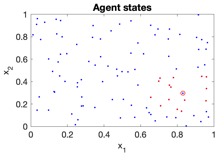
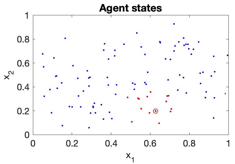
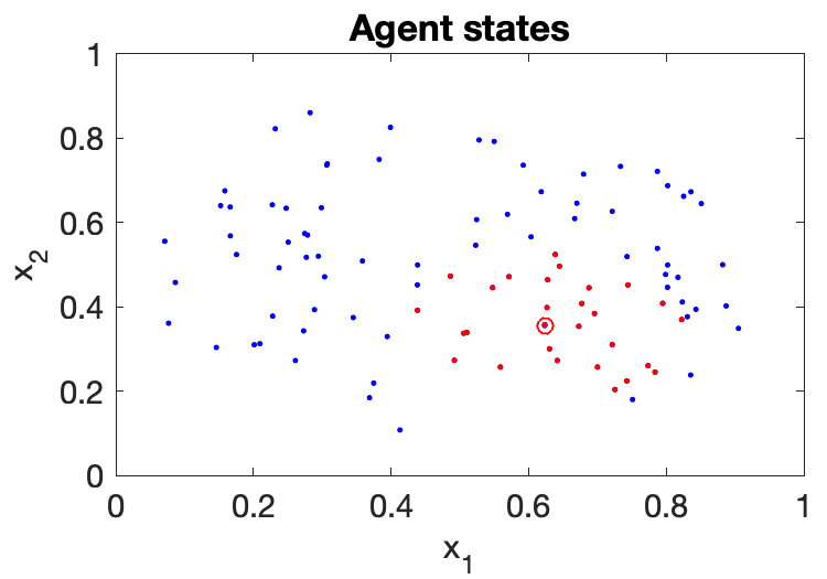
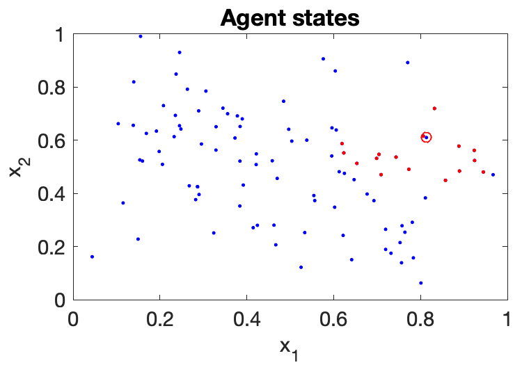

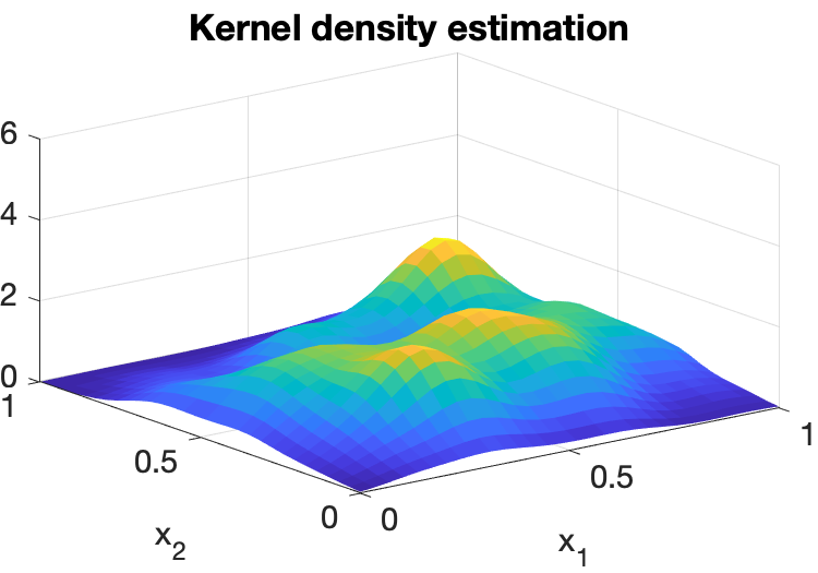
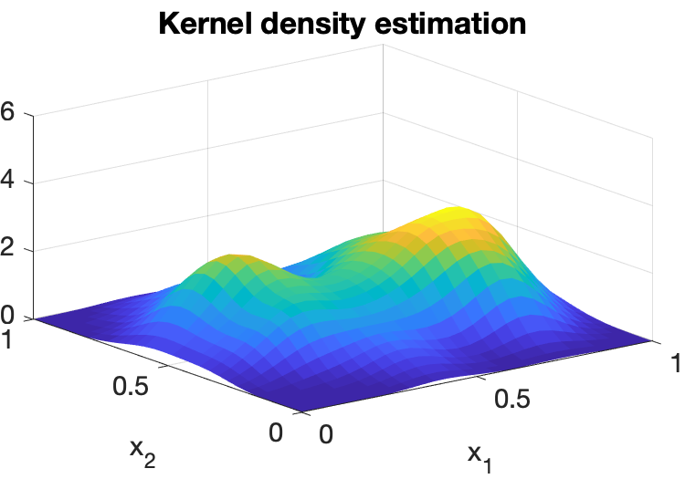
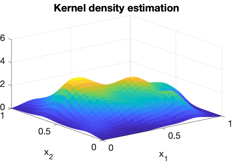
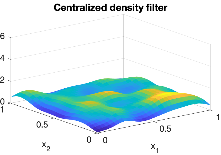
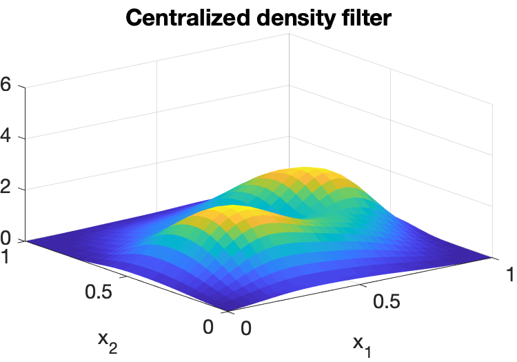
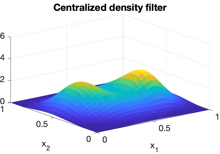
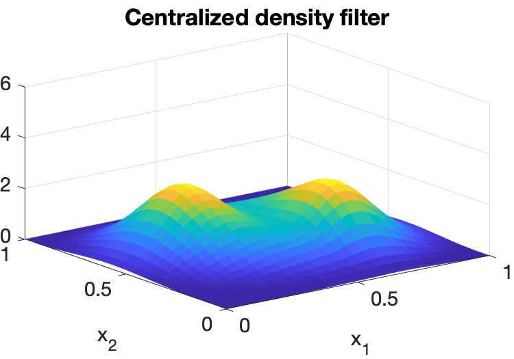
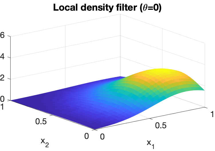
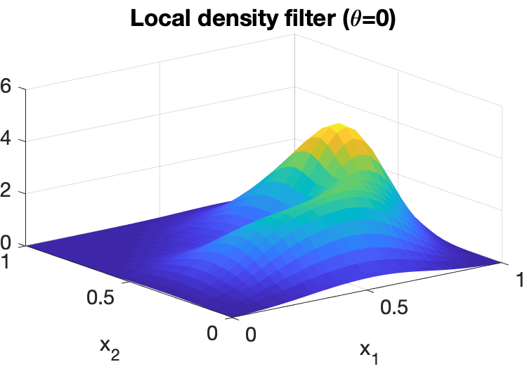
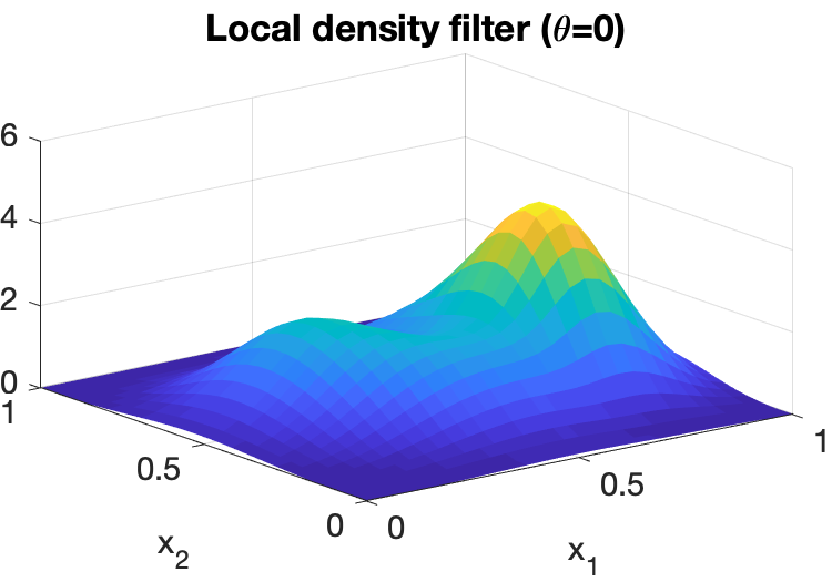
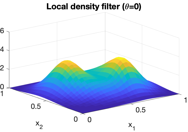

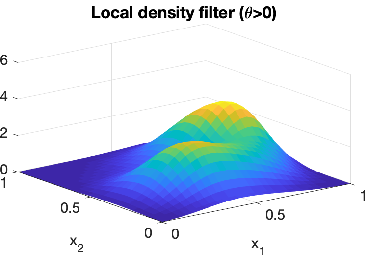
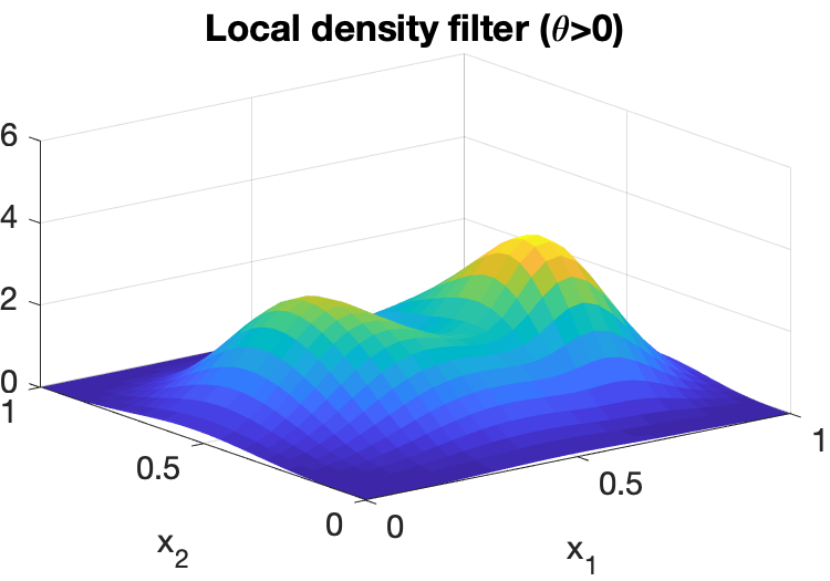
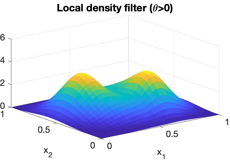
To verify the performance of the proposed centralized/distributed filters, we perform a simulation on Matlab using agents. The agents’ positions are generated by the following family of equations:
| (26) |
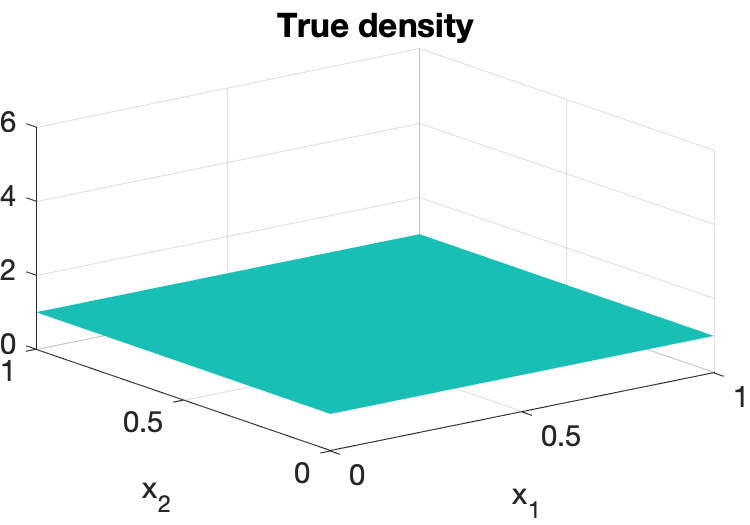
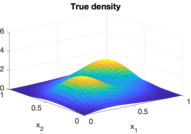
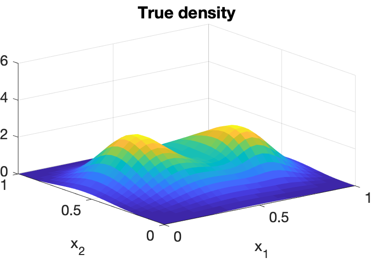
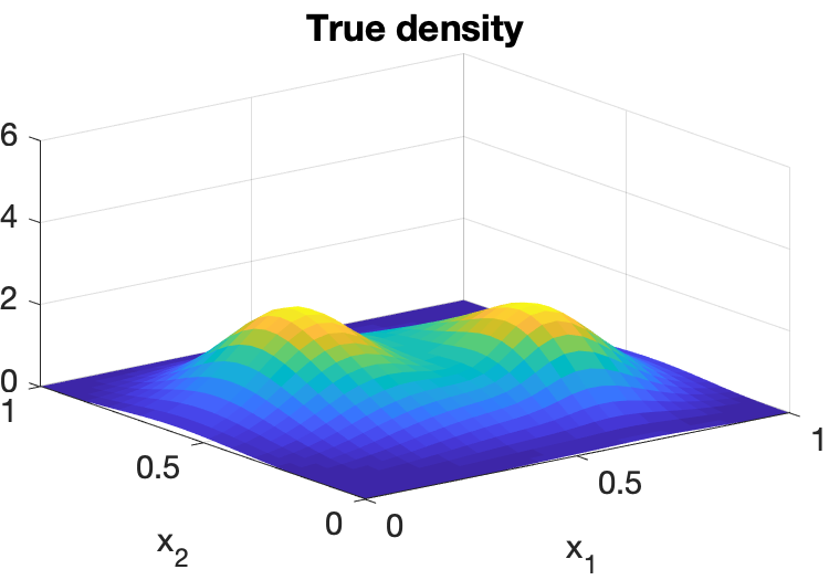
where and is a time-varying density function to be specified. We set with a reflecting boundary. The initial positions are drawn from the uniform distribution. Therefore, the ground truth density satisfies
| (27) | ||||
which will be used for comparison. We design to be a Gaussian mixture of two components with the common covariance matrix but different time-varying means and . Under this design, the agents are nonlinear and time-varying and their states will converge to two “spinning” Gaussian components.
The numerical implementation is based on the procedures outlined in Section 6. Specifically, is discretized as a grid. All density functions are approximated by vectors and all operators are approximated by matrices. The density updates and information exchange are performed in a synchronous manner with a step size . The bandwidth of KDE is . For the PI consensus algorithm (25), we set , , and .
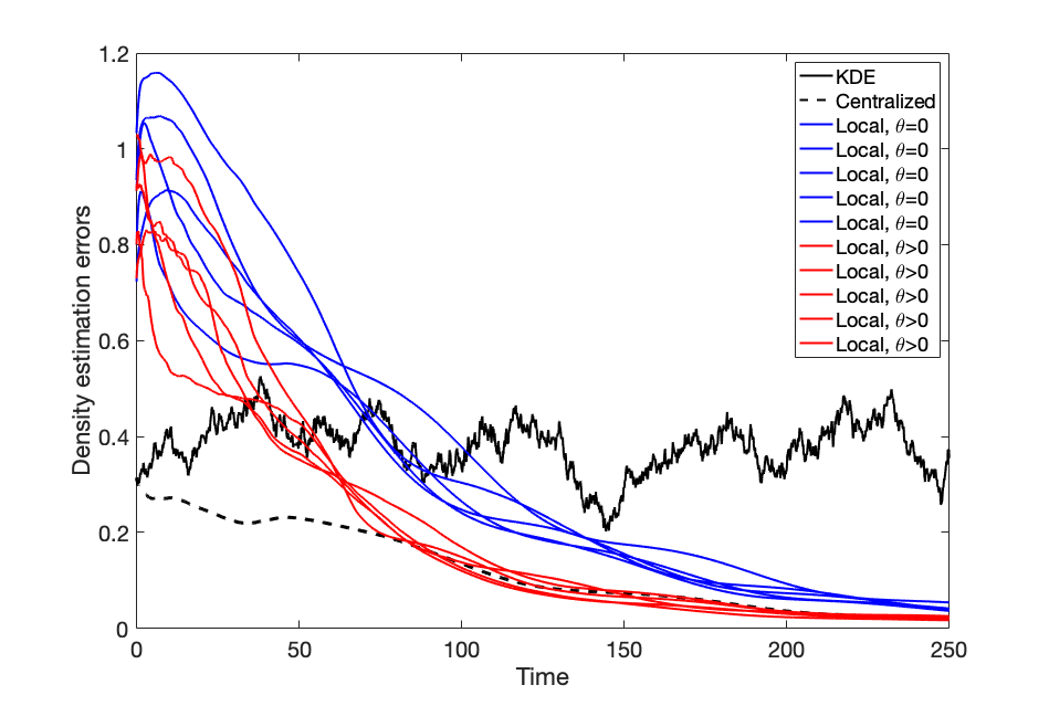
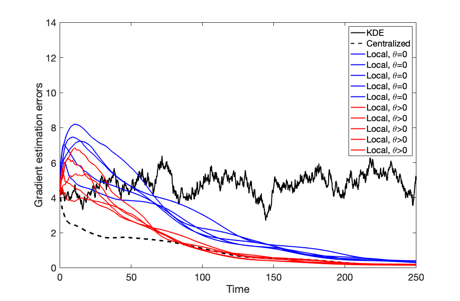
A graphical illustration of the simulation results is presented in Fig. 1, where each column represents the same time step and each row represents the evolution of an investigated quantity. As already observed in [19], the centralized filter, by taking advantage of the dynamics, quickly ”recognizes” the two underlying Gaussian components and gradually catches up with the evolution of the ground truth density, outperforming the outputs of KDE. Then, we randomly select an agent and investigate the performance of its local density filter when and . We observe that the two local filters also gradually catch up with the ground truth density, however in a slower rate compared with the centralized filter due to the delay effect of information exchange. In Fig. 2, we compare the norms of density and gradient estimation errors of KDE, the centralized filter, and 5 randomly selected local filters. We observe that all the filters outperform KDE as the filtering process proceeds. Both the density estimates and the gradient estimates are convergent. The local filters have larger initial density/gradient estimation errors because of limited observation on the initial step. Through information exchange, they gradually produce comparable performance with the centralized filter. In particular, the one with converges faster than the one with because of the additional exchange of density estimates with neighbors.
8 Conclusion
We presented centralized/distributed density filters for estimating the mean-field density of large-scale agent systems with known dynamics by a novel integration of mean-field models, KDE, infinite-dimensional Kalman filters, and communication protocols. With the distributed filter, each agent was able to estimate the global density using only the mean-field dynamics, its own state/position, and local information exchange with its neighbors. It was scalable to the number of agents, convergent in not only the density estimates but also their gradient, and efficient in terms of numerical implementation and communication. These algorithms can be used for many density-based distributed optimization and control problems of large-scale agent systems when density feedback information is required. Our future work is to integrate the density filters into mean-field feedback control for large-scale agent systems and study the closed-loop stability.
Appendices
8.1 Kernel density estimation
Kernel density estimation is a non-parametric way to estimate an unknown probability density function. Let be independent identically distributed random variables having a common probability density . The kernel density estimator for is given by [30, 10]
| (28) |
where is a kernel function [10] and is the bandwidth, usually chosen as a function of such that and . The Gaussian kernel is frequently used, given by
It is known that the is asymptotically normal and that and are asymptotically uncorrelated for , as , which is summarized as follows.
Lemma 8.23 (Asymptotic normality [31]).
If , then at any continuity point ,
| (29) |
If in addition , then as ,
| (30) |
in distribution, where represents the Gaussian distribution.
Lemma 8.24 (Asymptotic uncorrelatedness [31]).
Let be two distinct continuity points. If , then the covariance of and satisfies
These two lemmas together implies that as , the estimation error is asymptotically Gaussian with zero mean and diagonal covariance. Similar asymptotic normality and uncorrelatedness properties hold for the derivatives of [32]. In particular, as ,
| (31) | ||||
in distribution.
8.2 Generalized inverse operators
We introduce the notion of generalized inverse operators of self-adjoint operators defined in [33], which is based on an orthogonal decomposition. Let be a Hilbert space and be a self-adjoint operator, where represents the domain of . Let and to be the range and kernel of , respectively. Since is self-adjoint, (and we always have ). Thus, under the decomposition , we have the following representation for :
where is self-adjoint. Now, the generalized inverse is defined by:
with domain
We have the following facts:
(i) is self-adjoint.
(ii) One has that
(iii) The operator is an orthogonal projection onto . We may naturally extend it, still denoted it by itself, to . Hence, is the orthogonal projection onto . Similarly, we can extend to be an orthogonal projection from onto . Therefore, we have
8.3 Dynamic average consensus
We introduce the PI consensus estimator presented in [27]. Consider a group of agents where each agent has a local reference signal . The dynamic average consensus problem consists of designing an algorithm such that each agent tracks the time-varying average . The PI consensus algorithm is given by [27]:
| (32) |
where is agent ’s reference input, is an internal state, is agent ’s estimate of , and are adjacency matrices of the communication graph, and is a parameter determining how much new information enters the dynamic averaging process. The Laplacian matrices associated with and are represented by (proportional) and (integral) respectively. The PI estimator solves the consensus problem under constant (or slowly-varying) inputs, and remains stable for varying inputs in the sense of ISS. Define the tracking error of agent by . Decompose the error into the consensus direction and the disagreement directions orthogonal to . Define the transformation matrix where is such that . Consider the change of variables
to write (32) in the equivalent form
The stability result is given as follows.
Lemma 8.25.
[29] Let and be Laplacian matrices of strongly connected and weight-balanced digraphs. Then
where are constants depending on .
For switching networks, each switch introduces a transient to the estimator error, and is still ISS. The PI consensus estimator is also robust to initialization errors and permanent agent dropout in the sense that [29]:
| (33) |
References
- [1] J.-M. Lasry and P.-L. Lions, “Mean field games,” Japanese journal of mathematics, vol. 2, no. 1, pp. 229–260, 2007.
- [2] S. Ferrari, G. Foderaro, P. Zhu, and T. A. Wettergren, “Distributed optimal control of multiscale dynamical systems: a tutorial,” IEEE Control Systems Magazine, vol. 36, no. 2, pp. 102–116, 2016.
- [3] Y. Yang, R. Luo, M. Li, M. Zhou, W. Zhang, and J. Wang, “Mean field multi-agent reinforcement learning,” in International Conference on Machine Learning. PMLR, 2018, pp. 5571–5580.
- [4] K. Elamvazhuthi and S. Berman, “Mean-field models in swarm robotics: a survey,” Bioinspiration & Biomimetics, vol. 15, no. 1, p. 015001, 2019.
- [5] U. Eren and B. Açıkmeşe, “Velocity field generation for density control of swarms using heat equation and smoothing kernels,” IFAC-PapersOnLine, vol. 50, no. 1, pp. 9405–9411, 2017.
- [6] S. Bandyopadhyay, S.-J. Chung, and F. Y. Hadaegh, “Probabilistic and distributed control of a large-scale swarm of autonomous agents,” IEEE Transactions on Robotics, vol. 33, no. 5, pp. 1103–1123, 2017.
- [7] V. Krishnan and S. Martínez, “Distributed control for spatial self-organization of multi-agent swarms,” SIAM Journal on Control and Optimization, vol. 56, no. 5, pp. 3642–3667, 2018.
- [8] K. Elamvazhuthi, H. Kuiper, and S. Berman, “Pde-based optimization for stochastic mapping and coverage strategies using robotic ensembles,” Automatica, vol. 95, pp. 356–367, 2018.
- [9] T. Zheng, Q. Han, and H. Lin, “Transporting robotic swarms via mean-field feedback control,” IEEE Transactions on Automatic Control, (in press).
- [10] B. W. Silverman, Density Estimation for Statistics and Data Analysis. CRC Press, 1986, vol. 26.
- [11] R. D. Nowak, “Distributed em algorithms for density estimation and clustering in sensor networks,” IEEE transactions on signal processing, vol. 51, no. 8, pp. 2245–2253, 2003.
- [12] D. Gu, “Distributed em algorithm for gaussian mixtures in sensor networks,” IEEE Transactions on Neural Networks, vol. 19, no. 7, pp. 1154–1166, 2008.
- [13] Y. Hu, H. Chen, J.-g. Lou, and J. Li, “Distributed density estimation using non-parametric statistics,” in 27th International Conference on Distributed Computing Systems (ICDCS’07). IEEE, 2007, pp. 28–28.
- [14] S. J. Julier and J. K. Uhlmann, “Unscented filtering and nonlinear estimation,” Proceedings of the IEEE, vol. 92, no. 3, pp. 401–422, 2004.
- [15] Z. Chen et al., “Bayesian filtering: From kalman filters to particle filters, and beyond,” Statistics, vol. 182, no. 1, pp. 1–69, 2003.
- [16] R. Olfati-Saber, “Distributed kalman filtering for sensor networks,” in 2007 46th IEEE Conference on Decision and Control. IEEE, 2007, pp. 5492–5498.
- [17] S. Bandyopadhyay and S.-J. Chung, “Distributed estimation using bayesian consensus filtering,” in 2014 American control conference. IEEE, 2014, pp. 634–641.
- [18] G. Battistelli and L. Chisci, “Stability of consensus extended kalman filter for distributed state estimation,” Automatica, vol. 68, pp. 169–178, 2016.
- [19] T. Zheng, Q. Han, and H. Lin, “Pde-based dynamic density estimation for large-scale agent systems,” IEEE Control Systems Letters, vol. 5, no. 2, pp. 541–546, 2020.
- [20] T. Zheng and H. Lin, “Distributed density filtering for large-scale systems using mean-filed models,” in 2021 American Control Conference (ACC), 2021, pp. 334–339.
- [21] R. E. Kalman and R. S. Bucy, “New results in linear filtering and prediction theory,” Journal of basic engineering, vol. 83, no. 1, pp. 95–108, 1961.
- [22] A. Bensoussan, Filtrage optimal des systèmes linéaires. Dunod, 1971.
- [23] E. D. Sontag, “Smooth stabilization implies coprime factorization,” IEEE transactions on automatic control, vol. 34, no. 4, pp. 435–443, 1989.
- [24] S. Dashkovskiy and A. Mironchenko, “Input-to-state stability of infinite-dimensional control systems,” Mathematics of Control, Signals, and Systems, vol. 25, no. 1, pp. 1–35, 2013.
- [25] H. K. Khalil and J. W. Grizzle, Nonlinear systems. Prentice hall Upper Saddle River, NJ, 2002, vol. 3.
- [26] C. Villani, Optimal transport: old and new. Springer Science & Business Media, 2008, vol. 338.
- [27] R. A. Freeman, P. Yang, and K. M. Lynch, “Stability and convergence properties of dynamic average consensus estimators,” in Proceedings of the 45th IEEE Conference on Decision and Control. IEEE, 2006, pp. 338–343.
- [28] J. C. Strikwerda, Finite difference schemes and partial differential equations. SIAM, 2004.
- [29] S. S. Kia, B. Van Scoy, J. Cortes, R. A. Freeman, K. M. Lynch, and S. Martinez, “Tutorial on dynamic average consensus: The problem, its applications, and the algorithms,” IEEE Control Systems Magazine, vol. 39, no. 3, pp. 40–72, 2019.
- [30] E. Parzen, “On estimation of a probability density function and mode,” The annals of mathematical statistics, vol. 33, no. 3, pp. 1065–1076, 1962.
- [31] T. Cacoullos, “Estimation of a multivariate density,” Annals of the Institute of Statistical Mathematics, vol. 18, no. 1, pp. 179–189, 1966.
- [32] R. Singh, “Speed of convergence in nonparametric estimation of a multivariate -density and its mixed partial derivatives,” Journal of Statistical Planning and Inference, vol. 5, no. 3, pp. 287–298, 1981.
- [33] L. Mou and J. Yong, “Two-person zero-sum linear quadratic stochastic differential games by a hilbert space method,” Journal of Industrial & Management Optimization, vol. 2, no. 1, p. 95, 2006.