Bayesian estimation of the specific shear and bulk viscosity of the quark-gluon plasma with additional flow harmonic observables
Abstract
The transport properties of the strongly-coupled quark-gluon plasma created in ultra-relativistic heavy-ion collisions are extracted by Bayesian parameter estimate methods with the latest collision beam energy data from the CERN Large Hadron Collider. This Bayesian analysis includes sophisticated flow harmonic observables for the first time. We found that the temperature dependence of specific shear viscosity appears weaker than in the previous studies. The results prefer a lower value of specific bulk viscosity and a higher switching temperature to reproduce additional observables. However, the improved statistical uncertainties both on the experimental data and hydrodynamic calculations with additional observables do not help to reduce the final credibility ranges much, indicating a need for improving the dynamical collision model before the hydrodynamic takes place. In addition, the sensitivities of experimental observables to the parameters in hydrodynamic model calculations are quantified. It is found that the analysis benefits most from the symmetric cumulants and non-linear flow modes, which mostly reflect non-linear hydrodynamic responses, in constraining the temperature dependence of the specific shear and bulk viscosity in addition to the previously used flow coefficients.
I Introduction
The primary goal of heavy-ion physics is to investigate and understand the strongly coupled color-deconfined matter, quark-gluon plasma (QGP), which is produced in ultrarelativistic collisions between heavy ions. The QGP is believed to be the predominant form of matter during the first phases of the early universe. This matter behaves like a near-perfect fluid with the smallest specific shear viscosity, the ratio of the shear viscosity to the entropy density (), of any known substance in nature [1].
The most important remaining open questions in the field are the location of the critical point () in the QCD phase diagram and temperature dependence of specific shear () and bulk () viscosities of the QGP. The flow analysis in the Large Hadron Collider (LHC) has been very successful and provides valuable information to the field [2, 3, 4, 5, 6]. For example, the main constraints for the QGP properties using the Bayesian analysis [7] in the theory came from the ALICE measurements [8, 9, 2] with both low and high beam energy data. Even though the Bayesian analyses [7, 10, 11, 12, 13] were successful, the current uncertainties from these works are large because of statistical limitations of the data, limited observables used for the analysis, and computational constraints. In addition to the aforementioned limitations, pinning down the absolute value of at has a few challenges. First, a principle calculation to describe the initial conditions (IC) is still under development. Second, extracting the temperature dependence of has been complicated with the existence of the bulk viscosity [14, 15]. However, large flow found in small systems like proton-proton (pp) collisions was striking and opened up the importance of gluon fluctuations within protons and certainly, the experimental data would help to improve the understanding of IC both for small and large systems [16]. There are newer observables that give much stronger constraints to the theory [3, 4], showing good sensitivities especially to and . The correlation strength measured in [3, 4] was experimentally decomposed into two components of linear and non-linear flow modes in [17, 5] for the first time in the field, which gives a better understanding of our harmonic analysis and its origin with both LHC Run 1 (2009-2013) and Run 2 (2015-2018) data.
In this work, we extend the Bayesian parameter estimation methods employed in [7] with larger statistic LHC Run 2 results [18, 19] as well as a few additional observables [5, 6] for the first time which require substantial computational power. This work also allows us to quantify the sensitivity of each observable to the hydrodynamic model parameters in a controlled way. In Sec. II, we present a brief overview of Bayesian analysis methods and model setups. The experimental observables are described in Sec. III. Model parameters and calibrations are explained in Sec. IV. The results are presented in Sec. V, after which Sec. VI summarizes our results and findings.
II Bayesian analysis
There have been a number of studies that utilized Bayesian methods for heavy ion collisions [20, 21, 22, 23, 24]. We employ the recent state-of-the-art development in [7] for our present study. We define a vector of model parameters , and a set of experimental data that will be compared with model calculations. Bayes’s theorem gives the posterior distributions for the model parameters as
| (1) |
Here is the likelihood, which quantifies the model agreement with the data. The prior encapsulates initial knowledge on the parameters.
The model parameters are then extracted from the posterior distributions. We follow the same procedures as [7], where the model is first evaluated at a small number of ‘design’ parameter points. The resulting discrete set of model predictions is then made continuous by the use of a Gaussian process (GP) emulator, which thereby can be used to systematically probe the parameter space with Markov chain Monte-Carlo (MCMC) methods.
II.1 Hydrodynamic model and parameters
The model used in this analysis consists of the TRENTo model [25] for the initial condition, which is connected with free streaming to a 2+1 dimensional causal hydrodynamic model VISH(2+1) [26, 27]. The evolution continues after particlization via the UrQMD model [28, 29]. This hybrid model denoted TRENTo+VISH(2+1)+UrQMD, has successfully described the previous ALICE measurements [7].
A hydrodynamic modeling relies on the energy and momentum conservation laws of the fluid dynamics. The conservation is expressed in terms of
| (2) |
where is the energy-momentum tensor. In the case of viscous hydrodynamics, the energy-momentum tensor becomes
| (3) |
where is the energy density, is the local pressure given by the equation of state, and is a projector onto the transverse four-velocity. The shear- and bulk viscosities are encoded into and , respectively.
Free parameters of this model include the initial conditions, and , characterized by a total of 14 model parameters, which together control the prominent features of the model. The parameter set, described in detail in later sections, will enable simultaneous characterization of the initial state and medium response, including any correlations.
Each event consists of a single initial condition given energy density profile and a hydrodynamic simulation followed by multiple samples of the freeze-out hypersurface. The parameter estimation is conducted using 500 parameter design points, sampled evenly from the parameter space using the Latin hypercube scheme [30, 31]. At each design point, the model is used to generate around 3 events with the corresponding parametrization, with each event surface sampled ten times to produce a total of events for 0–60% centrality ranges. A large number of events is generated to ensure a better accuracy for high harmonic observables. A GP emulator is then trained to produce predictions for the observables in between the design points, after which the predictions are validated against a validation set. See [7] for details of the emulator. Using the emulator to produce predictions in continuous parameter space, the final posterior distribution is created using MCMC sampling.
II.2 Calibrating the model parameters
The parameter estimation attempts to calibrate the model parameters for the model to optimally reproduce experimental observables. With Bayesian methods, the optimal parameters are characterized by probability distributions for their true values. As given by Bayes’s theorem, the probability for the true parameters is
| (4) |
The left-hand side is the posterior: the probability of given the design , computed observables , and the experimental data . On the right-hand side, is the prior probability, encapsulating the initial knowledge of , and is the likelihood: the probability of observing given a proposal .
The likelihood may be computed using the principal component GP emulators as
| (5) |
where are the principal components predicted by the emulators, is the principal component transform of the experimental data , and is the covariance (uncertainty) matrix. The covariance matrix encodes all the experimental and model uncertainties [32]. In the principal component space, the covariance matrix can be expressed as
| (6) |
where is the matrix for experimental errors and is the diagonal GP emulator covariance matrix, representing the model statistical and GP predictive uncertainty. Additionally, is a free parameter ranging from zero to one, with the purpose of including all remaining uncertainties arising from the model imperfections. All model parameters are given a uniform prior. Together with the likelihood (5) and Bayes’ theorem (4), the posterior probability can evaluated at an arbitrary point in the parameter space. To construct the posterior distribution, an MCMC method can be used, which generates random walks through parameter space by accepting or rejecting proposal points based on the posterior probability.
III Experimental Observables
In the previous studies, the centrality dependence of identified particle yields and mean transverse momenta for charged pions, kaons, and protons as well as two-particle anisotropic flow coefficients for , 3, 4 were used. The observables are measured by the ALICE Collaboration in Pb–Pb collisions at TeV [8, 9, 2].
| Observable | Particle species | Kinematic cuts | Centrality classes | Ref. |
|---|---|---|---|---|
| Yields | , | 0–5, 5–10, 10–20, …, 50–60 | [18] | |
| Mean transverse momentum | , , | 0–5, 5–10, 10–20, …, 50–60 | [19] | |
| Two-particle flow cumulants | 0–5, 5–10, 10–20, …, 50–60 | [5] | ||
| GeV | ||||
| Non-linear flow mode | 0–5, 5–10, 10–20, …, 50–60 | [5] | ||
| GeV | ||||
| Symmetric cumulants | 0–5, 5–10, 10–20, …, 50–60 | [6] | ||
| GeV |

In this work, we mainly focus on the larger statistic higher beam energy collisions at TeV, which give better precision. In addition to the above mentioned observables, we include higher harmonic flow coefficients [5] (up to ), the normalized symmetric cumulants, [6], and the non linear flow mode coefficients [5].
The anisotropic pressure-driven expansion of the QGP, commonly referred to as anisotropic flow, can be characterized by a Fourier decomposition of the azimuthal particle distributions as
| (7) |
where quantifies the magnitude of the harmonic flow, and its direction. quantifies the correlations between event-by-event fluctuations of flow harmonics of different orders, [3, 6] and measures the contribution of lower order harmonic flows to higher order harmonics (i.e., is the non linear contribution of originating from ; see the details in [5]). These additional observables give better sensitivity to the medium properties and initial conditions as demonstrated in Refs. [3, 4, 5, 6].
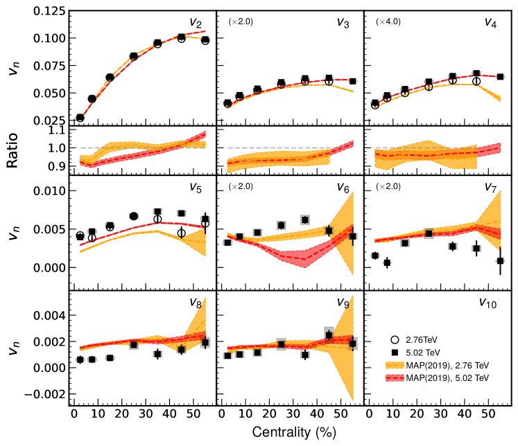
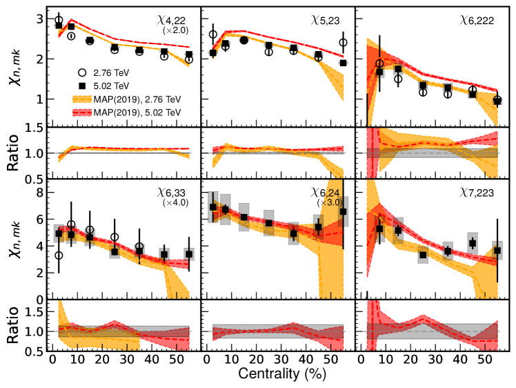
As shown in Fig. 1 and 2, a model calculation with the best-fit parametrization given by maximum a posteriori (MAP) from the previous Bayesian analysis [7] shows deviations of the measurements for the flow coefficients from and the non-linear flow mode coefficients from (). The black filled and open circles represent the higher () and lower () energy data points, respectively, whereas the red and orange bands represent the higher and lower energy model calculations. The values calculated from data were used in model calibration, and as seen in Fig. 1, the calculations agrees well for . However, a discrepancy is seen for with an underestimation of the calculations for the centrality up to for both energies, and an even larger discrepancy in for the higher energy calculation while the lower energy calculation agrees well except for the low centrality of . For higher harmonics () the deviation is still visible.
The model calculations for the non linear flow mode coefficients in Fig. 2 agree within for and for the higher energy model calculation of , while the lower energy model calculation goes to -30% in central collisions and even larger than 50% at high centrality ranges. The discrepancies between data and model calculations are significantly larger from ; however, for , most of the higher energy data points agree with the calculations within systematic uncertainties.
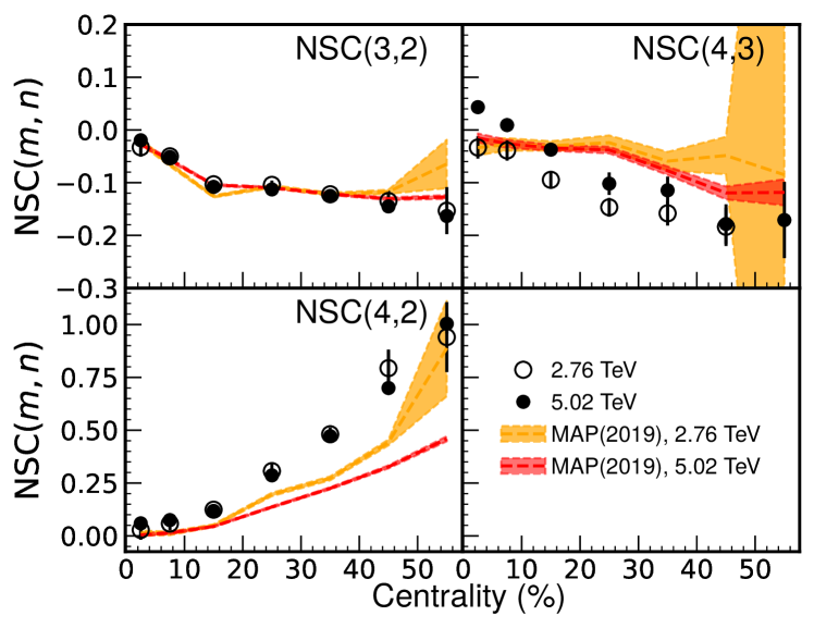
Model calculations reproduce the value for up to the centrality class, which is shown in Fig. 3. Both model predictions underestimate the values of for all centrality classes presented. The model calculations overestimate for the lower energy data and give similar results for the higher energy. However, the results show clear differences between the two beam energies. The differences get larger toward the central collisions. While it is negative for the lower energy data and the model calculations, the measurement at 5.02 TeV shows the change of the signs in central collisions. Also, the magnitudes are smaller in lower energy collisions, which is attributed to the increasing contribution from the nonlinear hydrodynamic response in [6].
In order to quantify the agreement of the models with the data, the test was performed in the same way as in Eq. (5) in Ref [4] for the centrality range 5–50%. The results are shown in Fig. 4 for the flow coefficients, non-linear flow mode coefficients, and the normalized symmetric cumulants. A significant difference is observed between the values for of higher and lower energies at . The values for are larger for both beam energies with similar magnitudes. The higher energy value for is significantly larger than the one from the lower energy as shown in Fig. 4. The disagreement is still significant for and . For , the values are larger for higher harmonics at both beam energies. The is especially large for the higher beam energy .
In our calculations of the observables, we used the same methods also used in experimental analysis in Refs. [3, 4, 5, 6]. Our centrality classes in this study are chosen to match those used for the experimental data. We define the multiplicity range for each centrality class by simulating events using the MAP-parametrization from [7], and sorting the resulting minimum-bias events by charged-particle multiplicity at midrapidity (). The identified and were evaluated by counting and averaging the particle species at midrapidity (). The experimental data are readily corrected and extrapolated to zero [9], and therefore no additional processing is required while preparing the comparison. For the identified , only protons were used in model calibration, as the model did not reproduce the spectra of the other species with any of the parametrizations. Finally, we calculated flow coefficients and other observables for charged particles within the kinematic range of the ALICE detector using the same methods as in the data analyses [5, 6]. A summary of all the observables that are included in the Bayesian analysis is given in Table 1. The table presents the particle species, kinematic cuts, and centrality classes for each observable.
IV Parameter estimation using new LHC measurements
| Parameter | Description | Range |
|---|---|---|
| Norm | Overall normalization | 16.542 – 25 |
| Entropy deposition parameter | 0.0042 – 0.0098 | |
| Std. dev. of nucleon multiplicity fluctuations | 0.5508 – 1.2852 | |
| Minimum volume per nucleon | – | |
| Free-streaming time | 0.03 – 1.5 | |
| Temperature of const. , | 0.135 – 0.165 | |
| Minimum | 0 – 0.2 | |
| Slope of above | 0 – 4 | |
| Curvature of above | – | |
| Temperature of maximum | 0.15 – 0.2 | |
| Maximum | 0 – 0.1 | |
| Width of peak | 0 – 0.1 | |
| Switching / particlization temperature | 0.135 – 0.165 |
The model to be evaluated in this analysis consists of multiple stages, of which a brief overview will be given next. Altogether, the model setup includes the parametric TRENTo initial conditions, free-streaming pre-equilibrium dynamics, and the VISH(2+1) hydrodynamic model for medium evolution. Furthermore, the model performs the hadronization and includes UrQMD hadronic cascade. The model setup used is identical to the one developed and used in [7], except for the number of hypersurface samples taken after evolution. In this work, exactly ten events are sampled from the hypersurface regardless of the cumulative number of particles. The centrality definition is shared for all parametrizations. With close to fixed initial stage parameters, the possible effects of a shared centrality definition should be negligible.
Our main focus will be to investigate the effects of the higher harmonic observables on the temperature dependence of the transport coefficients. The parametrizations of the transport coefficients are [7]
| (8) |
and
| (9) |
for the ratio of shear viscosity and bulk viscosity over entropy, respectively. Based on previous work, it is known that the lowest value of is around the critical temperature , close to the universal minimum . The temperature dependence of is moderate, and increasing with higher values of temperature. Within close proximity of to , the slope of is approximately linear. The bulk viscosity over entropy ratio is expected to peak around , and to decrease at higher values of temperature.
With this knowledge, we may construct our priori, and assume the initial parameter ranges. The chosen parameter ranges are loosely based on the optimal parameters found in [7]. It was found that in most cases, by taking the optimal parameters in [7] as the center points of the prior range and expanding the range slightly based on a reasonable value, those parameters could be further optimized with the additional observables. In this study, we have kept the initial stage parameter ranges narrow around the MAP values found in [7] with the assumption that the additional observables affect mostly the transport coefficients. Very small variation was allowed to give the parameters space to adjust for minor differences.
The included and varied parameters, of which there are 14 in total, are summarized in Table 2. The parametric TRENTo initial conditions comprise an ansatz in terms of five parameters: a normalization factor , entropy deposition parameter , standard deviation of the nuclear multiplicity fluctuations , Gaussian-shaped nucleon width , and minimum allowed distance between nucleons . The initial conditions are assumed to be already well constrained and presumably not affected by the addition of medium effect sensitive observables. The range for free-streaming time characterizing the allotted time for pre-equilibrium dynamics was kept relatively large.
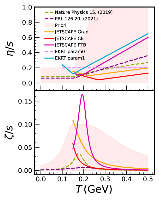
The rest of the parameters are the components of the transport coefficient parametrizations, and the switching temperature describing the temperature at which the hadronization begins to take place. The initial ranges given for these parameters are more generous, although large deviations in the final parameters compared to the previous study are not expected. The prior range for the transport coefficients is plotted in Fig. 5 among some parametrizations from other related studies [33, 34, 7, 13]. The parametrizations are valid only up to the corresponding limits of the model; in the case of EKRT and for JETSCAPE. We note that the parametrizations EKRT+param0 and EKRT+param1 were not obtained through Bayesian analysis and we do not consider the slightly higher at around in our prior. Furthermore, we do not consider the large reported with the PTB particlization by the JETSCAPE Collaboration [13]. Nevertheless, the obtained using the Grad or CE particlization distributions are within our prior, considering the temperature limit .
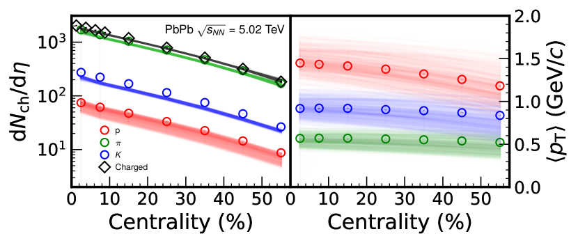
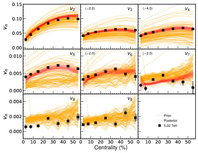
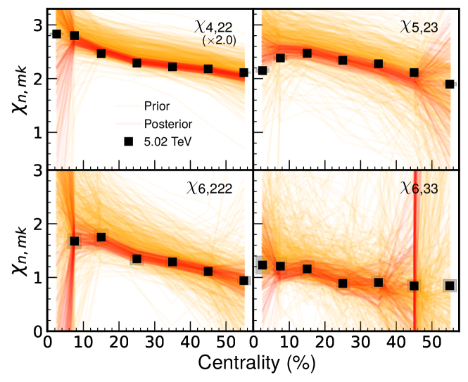
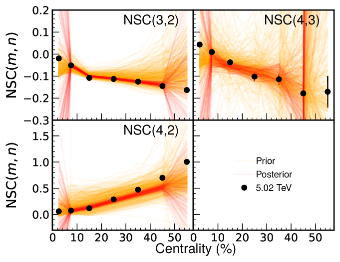
The model is calibrated to the latest Pb–Pb collision data at from the ALICE Collaboration [18, 19, 5, 6]. Figures 6–9 show the calculations of each observable using the design parametrizations obtained from the prior distribution. The yellow curves represent the calculations corresponding to each design point parametrization, which are used in training the GP emulator, whereas the red curves represent emulator predictions corresponding to random points sampled from the posterior distribution.
V Results
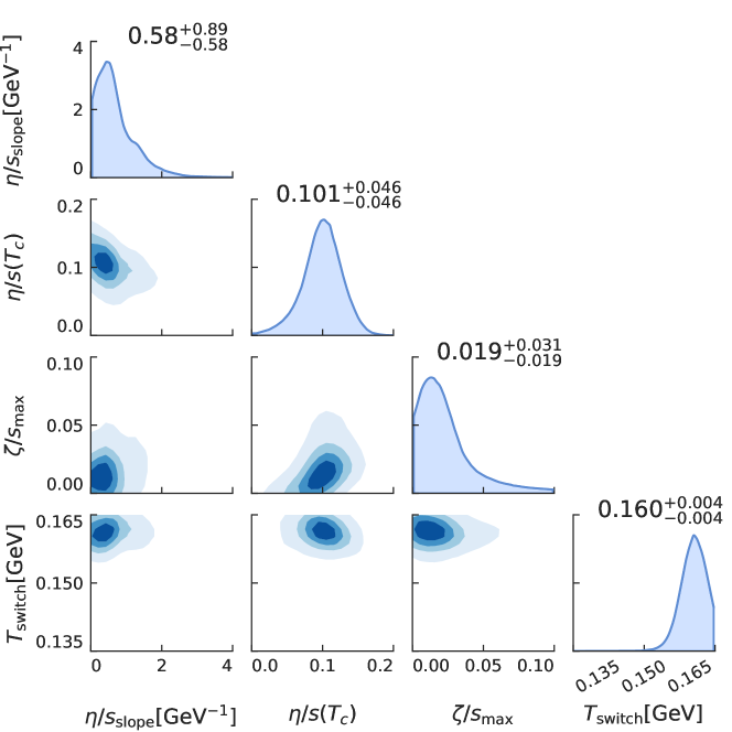
Figure 10 highlights the posterior and marginal distributions for select components of the transport parameters. The primary components, slope, , in the transport parametrizations are well constrained. The initial condition parameters are well constrained within the narrow prior range.
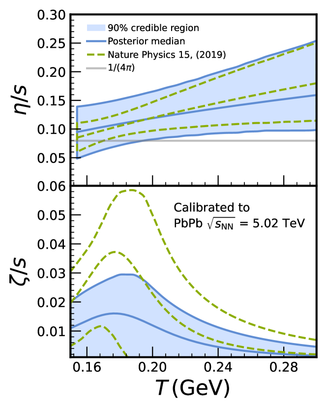
Figure 11 presents the estimated temperature dependence of and according to the parametrizations from Eqs. (8) and (9), respectively. The shaded region around the curves represents the 90%-credibility region. This region reflects all uncertainties coming from the finite width of the posterior distribution, experimental statistical and systematic uncertainties, statistical uncertainties in model calculations, predictive uncertainty from the GP emulator, and systematic model bias. With high probability, the true curve is located within this region.
Table 3 presents the best-fit MAP parameters from our analysis. We list here the important findings:
-
(i)
While the temperature dependence of is similar to what was obtained in [7], the curvature of is slightly stronger, resulting in lower values at higher temperatures above .
-
(ii)
A notable change is the lower in order to reproduce the additional observables. The obtained is smaller than those found in the previous Bayesian analyses [7, 13] where the additional observables were not included. A similar value was reported in Ref. [11]. On average this represents a value an order of magnitude lower compared to the lattice QCD calculation [35] and the parametrizations used in [36, 37], where the parametrizations were tuned to simultaneously reproduce lower harmonic as well as the charged particle multiplicity and the low- region of the charged hadron spectra.
-
(iii)
The switching temperature on the other hand is higher than the one found in the aforementioned studies, where on average is located around . As discussed in [4, 17, 5], the additional observables, the non linear response modes and the correlations between flow harmonics are sensitive to viscous corrections to the equilibrium distribution at hadronic freeze-out [38, 39, 40, 41] and seem to prefer the higher switching temperature.
| Initial conditions | Transport | ||
|---|---|---|---|
| Parameter | MAP value | Parameter | MAP value |
| Norm | 21.06 | 0.104 | |
| 0.0077 | 0.425 | ||
| 0.881 | -0.738 | ||
| 0.975 | 0.170 | ||
| 0.901 | 0.010 | ||
| 0.147 | 0.057 | ||
| 0.160 | |||
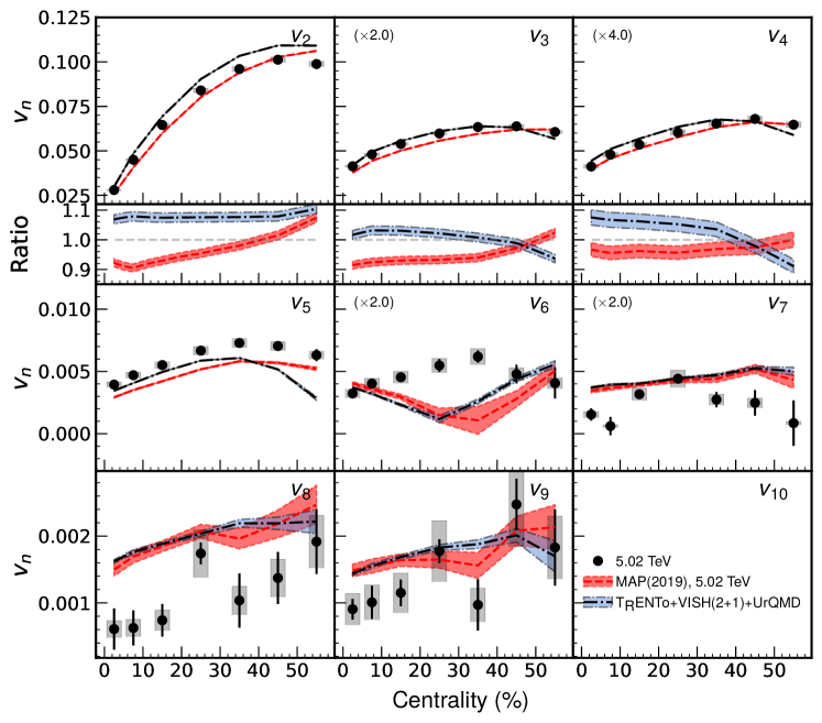
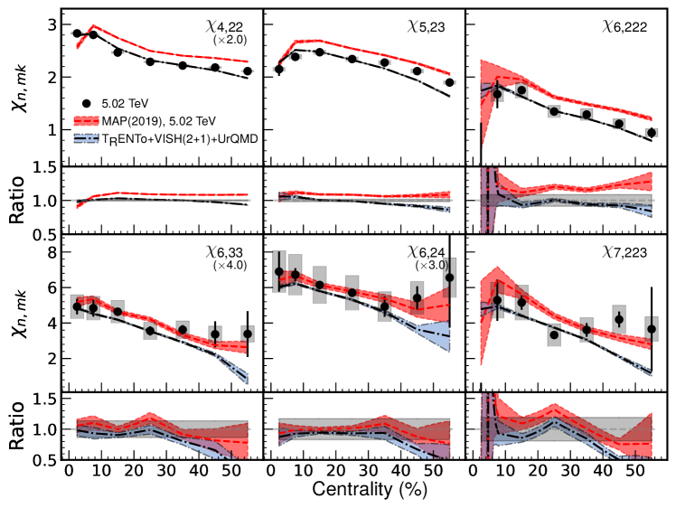
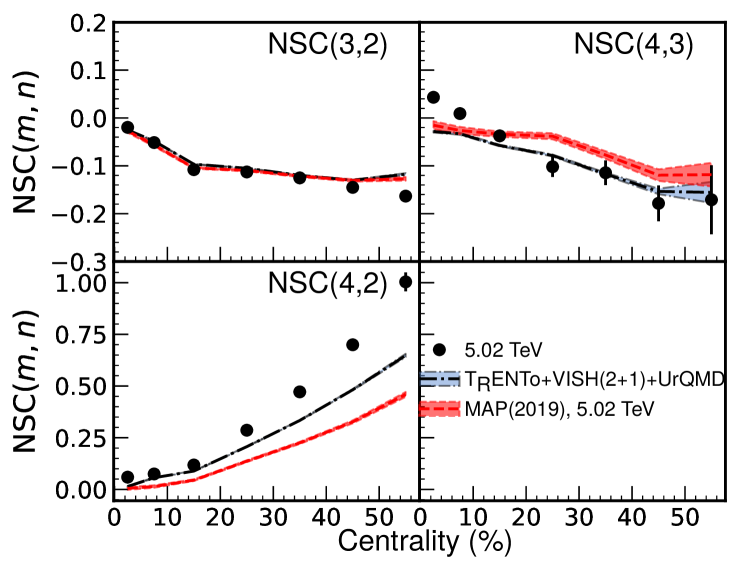
We performed high-statistics hydrodynamic calculations with the new parametrization. Figures 12 and 13 present the calculations for the flow coefficients and non linear flow mode coefficients, respectively. The is reproduced within 10% agreement for up to . For the fifth harmonic, the calculations underestimate the data. The new parametrization estimates the data better in central and peripheral collisions but deviates significantly in the peripheral region. The magnitude of the successive harmonics from is not quite captured by the calculations within the statistical uncertainty. Furthermore, with our new parametrization, the predictions for the non linear flow mode coefficients have also improved compared to the parametrization from [7], as indicated by the ratio plots. In this case, the lower harmonic non linear flow mode coefficients are no longer overestimated, and the magnitude and centrality dependence are correctly captured. We note that the non-linear flow mode coefficients have not been included in the model calibration in [7], whereas, coefficients up to and were used in this analysis. Figure 14 presents the calculation of the normalized SC using our obtained parametrization. The performance of the new parametrization and the one from [7] are comparable for NSC(3,2). For NSC(4,2) and NSC(4,3), the centrality dependence is better described by the new parametrization. However, both parametrizations are unable to reproduce the strong centrality dependence of NSC(4,2), underestimating the most data points in the most peripheral collisions.
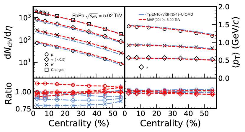

The multiplicity and the mean calculations are compared to the results from [7] in Fig. 15. Our parametrization improves the estimate of the proton multiplicity and gives the same charged particle multiplicity for 5.02 TeV collisions, while the pion and kaon multiplicities are not in good agreement with the experimental data, as similarly found in [7] for 2.76 TeV calculations. Interestingly, the parametrizations from [7] mainly utilizing 2.76 TeV data give better agreement with pions and kaons in 5.02 TeV collisions than our results while overestimating the proton yields approximately 10. Agreement of the calculated mean with the experimental data is good for all particle species as well as with the results from [7] for both beam energies. Refining this analysis by including low beam energy data in the future will help us to understand the beam energy dependence on various observables.
Finally, Fig. 16 shows the values with the best-fit MAP parameters extracted from this study for each observable. They are compared to the ones from [7]. The values for our new calculation only seem to improve and for the observable. For the non linear flow mode coefficients the values are improved up to with our new parametrization, while the values for the higher harmonics are worse than in [7]. For NSC, the from the new calculation is worse for NSC(3,2) and NSC(4,3), but is improved for NSC(4,2). We note that the larger statistical error in the calculations using the parametrization of Ref. [7] lowers the corresponding values, slightly affecting the direct comparison between the two parametrizations. The sign change of NSC(4,3) in most central collisions is not reproduced by the models while the beam energy-dependent magnitudes are better described with new parametrizations. We leave those differences for future research work where the present results should be refined by including experimental data from the lower energy beam data.
As a final study in this analysis, we conduct a simple sensitivity analysis of the included observables to the model transport parameters. The sensitivity of each observable is evaluated using the GP emulator by observing the relative difference in the magnitude of the observable between two parameter points in the parameter space. The difference can be formulated as
| (10) |
where and represent the values of an observable at parameter points and , respectively [13].
In this study, we choose a reference parameter point to be the one representing the MAP values obtained in this analysis (see Table 3). To probe the sensitivity of a parameter , another point is defined as , where is a small value representing a percentile change in the parameter space. We have used a value , although larger values were observed to yield similar results.
We then calculate a final sensitivity index for each observable and parameter pair in various centrality classes as
| (11) |
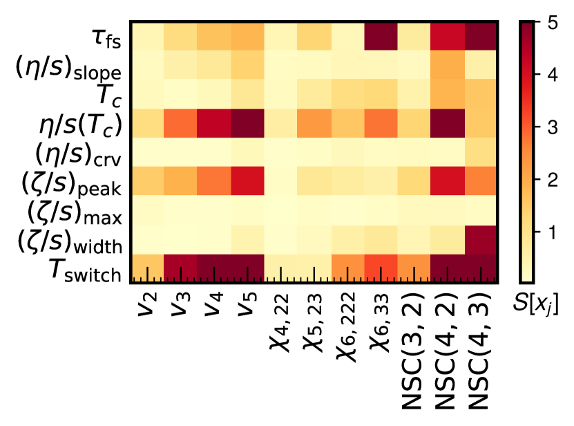
Figure 17 presents the evaluated sensitivity for each observable against the transport parameters. The sensitivity was evaluated over four centrality classes from 5% to 40% and averaged for the final plot. We did not observe large differences in the sensitivity between the individual centrality classes.
For , we can verify a known fact that the sensitivity of the flow coefficients is generally very limited to the temperature dependence of [33], although as expected, the sensitivity to the average , in this case, represented by , is very strong, and increasing at higher harmonics. The sensitivity of the to the is visible, and also in this case the higher harmonics provide stronger constraints. Based on previous studies, the non-linear flow mode coefficients are known to be sensitive to at the freeze-out temperature. This is reflected by the observed sensitivity to as well as . By far, the normalized symmetric cumulants provide the strongest constraints to the temperature dependence of . This is confirmed by higher sensitivity for the other components of , and not only , which is also higher.
Two other parameters have also been included in this study: the free-streaming time scale and the switching temperature . On average, the observables are reported to be generally weakly sensitive to , apart from the symmetric cumulants and . Furthermore, most of the observables, such as , and the m,n, are seen to be highly sensitive to the switching temperature . In both cases, the results reported here regarding and are not compatible with what has been observed in [13].
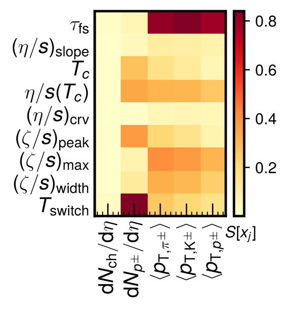
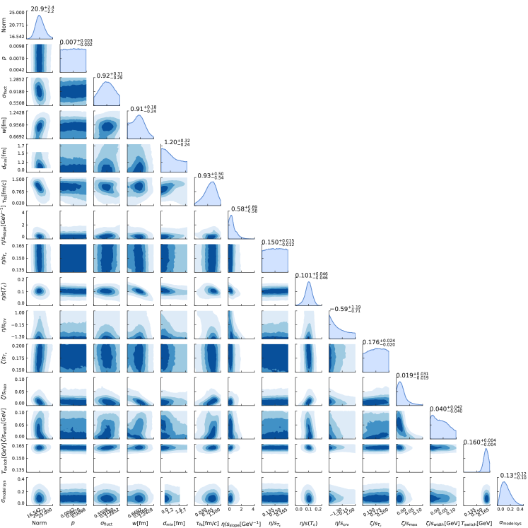
Figure 18 presents the sensitivity of the multiplicity and the to the model parametrizations. Most prominently, the switching temperature affects the proton multiplicity. Furthermore, we observe a comparatively large sensitivity of to the free-streaming time scale . In the case of the transport parameters, the effect on the observables is relatively small. It is observed that acts as a subtle constraint to the parameters describing the specific bulk viscosity. The posterior distribution for all parameters is shown in Fig. 19.
VI Discussions
In summary, we performed a Bayesian analysis with the recently available data from ALICE Collaboration [18, 19, 5, 6] as an extension of the work [7]. We found that the temperature dependence of is similar to what was obtained in [7] and that the curvature of above is slightly lower at higher temperatures, showing weak temperature dependence of . Notable changes include the lower and the higher switching temperature to reproduce additional observables such as symmetric cumulants and non-linear flow coefficients. However, the improved statistical uncertainties on both the experimental data and hydrodynamic calculations do not help to reduce the final credibility ranges. It is also noticeable that is still underestimated as observed in [7]. It is worthwhile to mention that the differences for , and NSC(4,2) still remain about 5–10% for 5.02 TeV. The sign change of NSC(4,3) in most central collisions is not reproduced by the models while the beam energy-dependent magnitudes are better described with new parametrizations. We leave those differences for future research work in which the present results should be refined by including the lower energy beam data. The parameter sensitivity analysis for the observables conducted in this study indicates that observables such as the symmetric cumulants and non linear flow modes provide a strong constraining power which, however, is still underutilized in [7] as well as the other Baysian analyses [10, 11, 13]. In our study, we confirm that the flow coefficients alongside the symmetric cumulants and non linear flow mode can provide some of the strongest constraints for the temperature dependence of and . Improving aspects of the collision model, for example by replacing the initial state model with others like EKRT [33, 34], IP-Glasma [42], and AMPT [43, 44] with incorporation of nucleon substructure [45] in the initial conditions through an improved dynamical collision model before the hydrodynamic takes place [46, 47], might help to improve the understanding of the uncertainties of the extracted QGP properties and/or the model building blocks.
Acknowledgements.
We would like to thank Harri Niemi, Kari J. Eskola and Sami Räsänen for fruitful discussions. We thank Jonah E. Bernhard, J. Scott Moreland and Steffen A. Bass for the use of their viscous relativistic hydrodynamics softwares and their valuable comments on various processes of this work. We acknowledge Victor Gonzalez for his crosscheck for various technical parts of the event generation. We acknowledge CSC - IT Center for Science in Espoo, Finland, for the allocation of the computational resources. This research was completed using million CPU hours provided by CSC.References
- Kovtun et al. [2005] P. Kovtun, D. T. Son, and A. O. Starinets, Viscosity in strongly interacting quantum field theories from black hole physics, Phys. Rev. Lett. 94, 111601 (2005), arXiv:hep-th/0405231 [hep-th] .
- Aamodt et al. [2011a] K. Aamodt et al. (ALICE), Higher harmonic anisotropic flow measurements of charged particles in Pb-Pb collisions at =2.76 TeV, Phys. Rev. Lett. 107, 032301 (2011a), arXiv:1105.3865 [nucl-ex] .
- Adam et al. [2016] J. Adam et al. (ALICE), Correlated event-by-event fluctuations of flow harmonics in Pb-Pb collisions at TeV, Phys. Rev. Lett. 117, 182301 (2016), arXiv:1604.07663 [nucl-ex] .
- Acharya et al. [2018] S. Acharya et al. (ALICE), Systematic studies of correlations between different order flow harmonics in Pb-Pb collisions at = 2.76 TeV, Phys. Rev. C97, 024906 (2018), arXiv:1709.01127 [nucl-ex] .
- Acharya et al. [2020a] S. Acharya et al. (ALICE), Higher harmonic non-linear flow modes of charged hadrons in Pb-Pb collisions at = 5.02 TeV, JHEP 05, 085, arXiv:2002.00633 [nucl-ex] .
- Acharya et al. [2021] S. Acharya et al. (ALICE), Measurements of mixed harmonic cumulants in Pb–Pb collisions at = 5.02 TeV, Phys. Lett. B 818, 136354 (2021), arXiv:2102.12180 [nucl-ex] .
- Bernhard et al. [2019] J. E. Bernhard, J. S. Moreland, and S. A. Bass, Bayesian estimation of the specific shear and bulk viscosity of quark-gluon plasma, Nature Physics 10.1038/s41567-019-0611-8 (2019).
- Aamodt et al. [2011b] K. Aamodt et al. (ALICE), Centrality dependence of the charged-particle multiplicity density at mid-rapidity in Pb-Pb collisions at TeV, Phys. Rev. Lett. 106, 032301 (2011b), arXiv:1012.1657 [nucl-ex] .
- Abelev et al. [2013] B. Abelev et al. (ALICE), Centrality dependence of , K, p production in Pb-Pb collisions at = 2.76 TeV, Phys. Rev. C 88, 044910 (2013), arXiv:1303.0737 [hep-ex] .
- Auvinen et al. [2020] J. Auvinen, K. J. Eskola, P. Huovinen, H. Niemi, R. Paatelainen, and P. Petreczky, Temperature dependence of of strongly interacting matter: Effects of the equation of state and the parametric form of , Phys. Rev. C 102, 044911 (2020), arXiv:2006.12499 [nucl-th] .
- Nijs et al. [2021a] G. Nijs, W. van der Schee, U. Gürsoy, and R. Snellings, A transverse momentum differential global analysis of Heavy Ion Collisions, Phys. Rev. Lett. 126, 202301 (2021a), arXiv:2010.15130 [nucl-th] .
- Nijs et al. [2021b] G. Nijs, W. van der Schee, U. Gürsoy, and R. Snellings, Bayesian analysis of heavy ion collisions with the heavy ion computational framework Trajectum, Phys. Rev. C 103, 054909 (2021b), arXiv:2010.15134 [nucl-th] .
- Everett et al. [2021] D. Everett et al. (JETSCAPE), Multisystem Bayesian constraints on the transport coefficients of QCD matter, Phys. Rev. C 103, 054904 (2021), arXiv:2011.01430 [hep-ph] .
- Ryu et al. [2018] S. Ryu, J.-F. Paquet, C. Shen, G. Denicol, B. Schenke, S. Jeon, and C. Gale, Effects of bulk viscosity and hadronic rescattering in heavy ion collisions at energies available at the BNL Relativistic Heavy Ion Collider and at the CERN Large Hadron Collider, Phys. Rev. C97, 034910 (2018), arXiv:1704.04216 [nucl-th] .
- Denicol et al. [2009] G. S. Denicol, T. Kodama, T. Koide, and P. Mota, Effect of bulk viscosity on Elliptic Flow near QCD phase transition, Phys. Rev. C80, 064901 (2009), arXiv:0903.3595 [hep-ph] .
- Acharya et al. [2019] S. Acharya et al. (ALICE), Investigations of Anisotropic Flow Using Multiparticle Azimuthal Correlations in pp, p-Pb, Xe-Xe, and Pb-Pb Collisions at the LHC, Phys. Rev. Lett. 123, 142301 (2019), arXiv:1903.01790 [nucl-ex] .
- Acharya et al. [2017] S. Acharya et al. (ALICE), Linear and non-linear flow modes in Pb-Pb collisions at 2.76 TeV, Phys. Lett. B773, 68 (2017), arXiv:1705.04377 [nucl-ex] .
- Adam et al. [2017] J. Adam et al. (ALICE), Centrality dependence of the pseudorapidity density distribution for charged particles in Pb-Pb collisions at TeV, Phys. Lett. B 772, 567 (2017), arXiv:1612.08966 [nucl-ex] .
- Acharya et al. [2020b] S. Acharya et al. (ALICE), Production of charged pions, kaons, and (anti-)protons in Pb-Pb and inelastic collisions at = 5.02 TeV, Phys. Rev. C 101, 044907 (2020b), arXiv:1910.07678 [nucl-ex] .
- Petersen et al. [2011] H. Petersen, C. Coleman-Smith, S. A. Bass, and R. Wolpert, Constraining the initial state granularity with bulk observables in Au+Au collisions at GeV, J. Phys. G38, 045102 (2011), arXiv:1012.4629 [nucl-th] .
- Novak et al. [2014] J. Novak, K. Novak, S. Pratt, J. Vredevoogd, C. Coleman-Smith, and R. Wolpert, Determining Fundamental Properties of Matter Created in Ultrarelativistic Heavy-Ion Collisions, Phys. Rev. C 89, 034917 (2014), arXiv:1303.5769 [nucl-th] .
- Pratt et al. [2015] S. Pratt, E. Sangaline, P. Sorensen, and H. Wang, Constraining the Eq. of State of Super-Hadronic Matter from Heavy-Ion Collisions, Phys. Rev. Lett. 114, 202301 (2015), arXiv:1501.04042 [nucl-th] .
- Sangaline and Pratt [2016] E. Sangaline and S. Pratt, Toward a deeper understanding of how experiments constrain the underlying physics of heavy-ion collisions, Phys. Rev. C93, 024908 (2016), arXiv:1508.07017 [nucl-th] .
- Heinz and Liu [2015] U. W. Heinz and J. Liu, Pre-equilibrium dynamics and heavy-ion observables, in 25th International Conference on Ultra-Relativistic Nucleus-Nucleus Collisions (Quark Matter 2015) Kobe, Japan, September 27-October 3, 2015 (Nucl. Phys. A, in press, 2015) arXiv:1512.08276 [nucl-th] .
- Moreland et al. [2015] J. S. Moreland, J. E. Bernhard, and S. A. Bass, Alternative ansatz to wounded nucleon and binary collision scaling in high-energy nuclear collisions, Phys. Rev. C92, 011901 (2015), arXiv:1412.4708 [nucl-th] .
- Shen et al. [2016] C. Shen, Z. Qiu, H. Song, J. Bernhard, S. Bass, and U. Heinz, The iEBE-VISHNU code package for relativistic heavy-ion collisions, Comput. Phys. Commun. 199, 61 (2016), arXiv:1409.8164 [nucl-th] .
- Song and Heinz [2008] H. Song and U. W. Heinz, Causal viscous hydrodynamics in 2+1 dimensions for relativistic heavy-ion collisions, Phys. Rev. C 77, 064901 (2008), arXiv:0712.3715 [nucl-th] .
- Bass et al. [1998] S. A. Bass et al., Microscopic models for ultrarelativistic heavy ion collisions, Prog. Part. Nucl. Phys. 41, 255 (1998), arXiv:nucl-th/9803035 .
- Bleicher et al. [1999] M. Bleicher et al., Relativistic hadron hadron collisions in the ultrarelativistic quantum molecular dynamics model, J. Phys. G 25, 1859 (1999), arXiv:hep-ph/9909407 .
- Tang [1993] B. Tang, Orthogonal array-based latin hypercubes, Journal of the American Statistical Association 88, 1392 (1993).
- Morris and Mitchell [1995] M. D. Morris and T. J. Mitchell, Exploratory designs for computational experiments, Journal of Statistical Planning and Inference 43, 381 (1995).
- Bernhard [2018] J. E. Bernhard, Bayesian parameter estimation for relativistic heavy-ion collisions, Ph.D. thesis, Duke U. (2018), arXiv:1804.06469 [nucl-th] .
- Niemi et al. [2016a] H. Niemi, K. J. Eskola, and R. Paatelainen, Event-by-event fluctuations in a perturbative QCD + saturation + hydrodynamics model: Determining QCD matter shear viscosity in ultrarelativistic heavy-ion collisions, Phys. Rev. C93, 024907 (2016a), arXiv:1505.02677 [hep-ph] .
- Niemi et al. [2016b] H. Niemi, K. J. Eskola, R. Paatelainen, and K. Tuominen, Predictions for 5.023 TeV Pb + Pb collisions at the CERN Large Hadron Collider, Phys. Rev. C93, 014912 (2016b), arXiv:1511.04296 [hep-ph] .
- Nakamura and Sakai [2005] A. Nakamura and S. Sakai, Transport coefficients of gluon plasma, Phys. Rev. Lett. 94, 072305 (2005), arXiv:hep-lat/0406009 .
- McDonald et al. [2017] S. McDonald, C. Shen, F. Fillion-Gourdeau, S. Jeon, and C. Gale, Hydrodynamic predictions for Pb+Pb collisions at 5.02 TeV, Phys. Rev. C95, 064913 (2017), arXiv:1609.02958 [hep-ph] .
- Zhao et al. [2017] W. Zhao, H.-j. Xu, and H. Song, Collective flow in 2.76 A TeV and 5.02 A TeV Pb+Pb collisions, Eur. Phys. J. C77, 645 (2017), arXiv:1703.10792 [nucl-th] .
- Luzum and Ollitrault [2010] M. Luzum and J.-Y. Ollitrault, Constraining the viscous freeze-out distribution function with data obtained at the BNL Relativistic Heavy Ion Collider (RHIC), Phys. Rev. C 82, 014906 (2010), arXiv:1004.2023 [nucl-th] .
- Luzum et al. [2010] M. Luzum, C. Gombeaud, and J.-Y. Ollitrault, in ideal and viscous hydrodynamics simulations of nuclear collisions at the BNL Relativistic Heavy Ion Collider (RHIC) and the CERN Large Hadron Collider (LHC), Phys. Rev. C 81, 054910 (2010), arXiv:1004.2024 [nucl-th] .
- Teaney and Yan [2012] D. Teaney and L. Yan, Non linearities in the harmonic spectrum of heavy ion collisions with ideal and viscous hydrodynamics, Phys. Rev. C 86, 044908 (2012), arXiv:1206.1905 [nucl-th] .
- Yan and Ollitrault [2015] L. Yan and J.-Y. Ollitrault, : nonlinear hydrodynamic response versus LHC data, Phys. Lett. B744, 82 (2015), arXiv:1502.02502 [nucl-th] .
- Schenke et al. [2012] B. Schenke, P. Tribedy, and R. Venugopalan, Fluctuating Glasma initial conditions and flow in heavy ion collisions, Phys. Rev. Lett. 108, 252301 (2012), arXiv:1202.6646 [nucl-th] .
- Bhalerao et al. [2015] R. S. Bhalerao, A. Jaiswal, and S. Pal, Collective flow in event-by-event partonic transport plus hydrodynamics hybrid approach, Phys. Rev. C92, 014903 (2015), arXiv:1503.03862 [nucl-th] .
- Pang et al. [2012] L. Pang, Q. Wang, and X.-N. Wang, Effects of initial flow velocity fluctuation in event-by-event (3+1)D hydrodynamics, Phys. Rev. C86, 024911 (2012), arXiv:1205.5019 [nucl-th] .
- Mäntysaari et al. [2017] H. Mäntysaari, B. Schenke, C. Shen, and P. Tribedy, Imprints of fluctuating proton shapes on flow in proton-lead collisions at the LHC, Phys. Lett. B 772, 681 (2017), arXiv:1705.03177 [nucl-th] .
- van der Schee et al. [2013] W. van der Schee, P. Romatschke, and S. Pratt, Fully Dynamical Simulation of Central Nuclear Collisions, Phys. Rev. Lett. 111, 222302 (2013), arXiv:1307.2539 [nucl-th] .
- Romatschke and Romatschke [2019] P. Romatschke and U. Romatschke, Relativistic Fluid Dynamics In and Out of Equilibrium, Cambridge Monographs on Mathematical Physics (Cambridge University Press, 2019) arXiv:1712.05815 [nucl-th] .