Fast estimation of aperture-mass statistics II: Detectability of higher order statistics in current and future surveys

Abstract

We explore an alternative method to the usual shear correlation function approach for the estimation of aperture mass statistics in weak lensing survey data. Our approach builds on the direct estimator method. In this paper, we extend our analysis to statistics of arbitrary order and to the multiscale aperture mass statistics. We show that there always exists a linear order algorithm to retrieve any of these generalised aperture mass statistics from shape catalogs when the direct estimator approach is adopted. We validate our approach through application to a large number of Gaussian mock lensing surveys where the true answer is known and we do this up to 10th order statistics. We then apply our estimators to an ensemble of real-world mock catalogs obtained from $N$-body simulations – the SLICS mocks, and show that one can expect to retrieve detections of higher order clustering up to fourth order in a KiDS-1000 like survey. We expect that these methods will be of most utility for future wide-field surveys like Euclid and the Rubin Telescope.

1 Introduction

Weak gravitational lensing by large-scale structure of the light from distant galaxies is a powerful probe for constraining the cosmological parameters and distinguishing between competing models of the Universe (Blandford et al., 1991; Seitz et al., 1994; Jain & Seljak, 1997; Kaiser, 1998; Schneider et al., 1998; Zhang et al., 2007). The first measurements of the correlations in the shapes of distant background galaxies date back more than two decades (Bacon et al., 2000; Kaiser et al., 2000; Van Waerbeke et al., 2000; Wittman et al., 2000). Since then, cosmic shear observations have become ever more precise as the coupling of techological advancements and algorithmic developments have enabled us to conduct unprecedented deep optical imaging surveys of the cosmos KiDS, DES and HSC, with current state-of-the-art surveys now mapping thousands of square degrees (Hildebrandt et al., 2017; Troxel et al., 2018; Aihara et al., 2018; Hikage et al., 2019; Asgari et al., 2021). By the end of the decade planned experiments like Euclid and the Rubin Telescope (Laureijs et al., 2011; LSST, 2009) will map volumes close to the entire physical volume of our observable Universe. In order to make optimal use of these rich data sets we will need to push forward our understanding and modelling of various physical and measurement effects. In particular: accurate modelling of the nonlinear evolution of large-scale structure, including the baryonic physics effects; accurate modelling and correction of the point-spread function of the telescope; correcting the bias in the weak lensing shape estimation algorithms; and accounting for the intrinsic alignments, to name but a few of the main systematics (see Schneider, 2006b; Massey et al., 2013; Troxel & Ishak, 2015, for a more detailed discussion of these effects).

If the underlying matter density field were a Gaussian random field, then all of the information in a weak lensing survey would be contained in the shear two-point correlation function. However, physical effects like: the nonlinear growth of structure (Bernardeau et al., 2002), the mapping between cosmic shear and galaxy ellipticities (Miralda-Escude, 1991), and lensing beyond the Born approximation (Hilbert et al., 2009; Pratten & Lewis, 2016; Fabbian et al., 2018), all introduce non-Gaussianity in the maps. Furthermore, the nonlinear evolution also induces correlations in the convergence power spectrum multipoles, which grow stronger on small scales. This means that the information content of the second order statistics becomes saturated after a given multipole (Sato et al., 2011; Hilbert et al., 2012; Kayo et al., 2013; Marian et al., 2013; Byun et al., 2017). Thus in order to capture all of the cosmological information available in lensing surveys one must look to the higher order statistics of the shear field (Schneider et al., 1998; Bernardeau et al., 2002; Schneider & Lombardi, 2003). Furthermore, owing to the different ways in which the cosmological parameters and nuisance parameters depend on the higher-order statistics, the inclusion of such measurements brings with it the further virtue of being able to break parameter degeneracies, e.g. by combining second and third order statistics (Kilbinger & Schneider, 2005; Semboloni et al., 2011; Fu et al., 2014), or by incorporating the information found in the statistical properties of the peaks in the shear field (Marian et al., 2013; Kacprzak et al., 2016).

A powerful method to disentangle systematic effects from cosmic shear signals is the E/B decomposition (Crittenden et al., 2001; Schneider et al., 2002a). At leading order, pure weak lensing signals are sourced by a scalar lensing potential, which means that their deflection fields are curl free. Equivalently, the ring-averaged cross component of the shear is expected to be zero (the B mode), while the tangential one contains all the lensing signal (the E mode). Thus B modes enable a robust test for the presence of systematic errors. One method to take advantage of this E/B decomposition is the so-called ‘aperture mass statistics’ (Kaiser, 1995; Schneider, 1996; Schneider et al., 1998). ‘Aperture mass’ (${\mathcal{M}}_{\rm ap}$) and ‘Map-Cross’ $(\mathcal{M}_{\times})$ are obtained by convolving the tangential and cross shear with an isotropic filter function. Therefore by construction they are E/B-decomposed. Taking the second moment leads to the variance of aperture mass, the third to the skewness, the fourth to the kurtosis, etc.

The standard approach for measuring the aperture mass statistics in data utilises the fact that, for the flat sky, any $n$-point moment can be expressed in terms of integrals over the $n$-point shear correlation functions, modulo a kernel function (Schneider et al., 2002a; Jarvis et al., 2004). The reason for adopting this strategy stems from the fact that the correlation functions can reliably be estimated in the presence of a nontrivial survey mask. However, for these estimators to be accurate and E/B decomposed, one requires three conditions to be satisfied: (i) the $\xi_{+}$/$\xi_{-}$ correlations need to be measured down to zero separation; (ii) they also need to be measured up to a maximum angular scale, set by the exact form of the aperture mass filter and its angular scale; (iii) the angular bins must be sufficiently fine for the discretisation of the integrals to be reliable (Kilbinger & Schneider, 2005; Fu et al., 2014). Owing to galaxy image blending, signal-to-noise issues and the finite size of the survey, the lower bound is never possible and the upper bound means that biases can occur due to edge effects. In addition, while the mean estimate is unbiased, the covariance matrix does require one to carefully account for the mask (Schneider et al., 2002b; Friedrich et al., 2016). More recent developments that also make use of the shear correlation functions, while circumventing the issues of E/B leakage on small scales are the ring statistics and COSEBIs (Schneider & Kilbinger, 2007; Schneider et al., 2010). While those approaches can in principle be extended to higher order statistics, the estimation of the $n$-point correlation functions turns out to be notoriously time consuming (Schneider et al., 2005; Jarvis et al., 2003). Further methods to extract non-Gaussian information from the aperture mass look at its probability density function as a whole (Bernardeau & Valageas, 2000; Munshi et al., 2004; Barthelemy et al., 2020) or at the distribution of its signal-to-noise peaks (Marian et al., 2012; Heydenreich et al., 2020; Martinet et al., 2021).

In Porth et al. (2020) we took a different approach and explored a computationally efficient (accelerated) implementation of the original direct estimator of the aperture mass dispersion (Schneider, 1998). Rather than measuring the correlation functions of the shear polar, in this formulation one instead directly measures cumulants of $\mathcal{M}_{\rm ap}$ on a set of apertures and then uses an optimised weighting scheme to average the estimates, along with a restriction on the types of apertures that are acceptable. The present work extends our previous investigation in a number of important ways. First, we construct accelerated direct estimators for the higher-order aperture mass moments, including the skewness, kurtosis, etc. Second, we also develop further the multiscale aperture moments (Jarvis et al., 2003; Schneider et al., 2005). These two improvements enable us to better trace the full, harmonic mode, configuration dependence of the convergence polyspectra.

This paper is organised as follows: In §2 we introduce key concepts of weak lensing, define the aperture mass and show how its connected cumulants are related to the convergence polyspectra. In §3 we revisit the direct estimators for higher order aperture mass measures and construct suitable bases, in which each statistic can be computed in linear time complexity. After investigating the variance of the direct estimators, we give details of our updated algorithm used to perform the measurements. In §4 we empirically verify the linear scaling and the measurements of our implementation of the direct estimator on Gaussian mocks. In §5 we then apply the estimator to the SLICS simulation suite in order to assess up to which order one can expect to extract information from the aperture mass statistics on a KiDS-1000 like survey. Finally, in §6 we summarise our findings, conclude and discuss future work.

2 Higher order aperture mass measures for cosmic shear

2.1 Weak gravitational lensing and aperture mass

In this paper we are mainly concerned with the weak lensing of distant background (source) galaxy shapes by the intervening large-scale structure (for detailed reviews of the topic see Bartelmann & Schneider, 2001; Schneider, 2006a, b; Dodelson, 2003, 2017; Kilbinger, 2015; Mandelbaum, 2018). The two fundamental quantities describing this mapping from true to observed galaxy images are the convergence $\kappa$ and the complex shear $\gamma=\gamma_{1}+i\gamma_{2}$, which, assuming a metric theory of gravity, are all derived from an underlying scalar lensing potential. In a galaxy survey the effective convergence at angular position $\bm{\theta}$ and radial comoving distance $\chi$ can be connected to the density contrast $\delta(\chi\bm{\theta},\chi)$ through:

$$\kappa({\bm{\theta}}) =\frac{3}{2}\Omega_{\rm m,0}\left(\frac{H_{0}}{c}\right)^{2}\int_{0}^{\chi_{\rm H}}{\rm d}\chi^{\prime}\frac{\chi^{\prime}}{a(\chi^{\prime})}g(\chi^{\prime})\delta(\chi^{\prime}{\bm{\theta}},\chi^{\prime})\ ,$$ (1)

where $\Omega_{\rm m,0}$ is the total matter density, $H_{0}$ denotes the Hubble constant, $a$ is the scale factor, $c$ is the speed of light, $\chi_{H}$ is the comoving distance to the horizon and $g(\chi)$ is a weight function related to the normalized redshift distribution ${\rm d}n(z)/{\rm d}z$ of the source galaxies as

$$g(\chi^{\prime}) \equiv\int_{z(\chi^{\prime})}^{z_{\rm H}}{\rm d}z\ \frac{{\rm d}n(z)}{{\rm d}z}\frac{\left[\chi(z)-\chi^{\prime}\right]}{\chi(z)}\ .$$ (2)

Aperture mass was developed by Schneider (1996) as a technique to estimate projected mass overdensities enclosed within a circular region:

$${\mathcal{M}}_{\rm ap}({\bm{\theta}}_{0};{\vartheta})=\int_{{\mathbb{R}^{2}}}{{\rm d}^{2}\bm{\theta}}_{1}\kappa({\bm{\theta}}_{1})U(\left|{\bm{\theta}}_{1}-{\bm{\theta}}_{0}\right|;{\vartheta})\ ,$$ (3)

where $U$ is a compensated filter function. In the flat sky limit the (cross) aperture mass can be expressed in terms of a related circularly symmetric filter function $Q(U)$ and the complex shear field $\gamma$ in its E/B-decomposed basis:

$$\mathcal{M}_{{\rm ap}/\times}({\bm{\theta}}_{0};{\vartheta})\equiv\int_{{\mathbb{R}^{2}}}{{\rm d}^{2}\bm{\theta}}_{1}\gamma_{{\rm t}/\times}({\bm{\theta}}_{1};{\bm{\theta}}_{0})Q(|{\bm{\theta}}_{1}-{\bm{\theta}}_{0}|;{\vartheta})\ ,$$ (4)

where the tangential and cross components of the shear field at position ${\bm{\theta}}+{\bm{\theta}}_{0}$ with respect to the aperture center ${\bm{\theta}}_{0}$ are defined as (Bartelmann & Schneider, 2001):

$$\gamma_{\rm t}({\bm{\theta}};{\bm{\theta}}_{0})+i\gamma_{\times}({\bm{\theta}};{\bm{\theta}}_{0}) \equiv-\gamma(\bm{\theta}+{\bm{\theta}}_{0}){\rm e}^{-2i\phi}\ ,$$ (5)

in which $\phi$ denotes the polar angle associated with the vector ${\bm{\theta}}$. In the absence of systematic errors (B-modes) in the lensing data, map-cross should vanish (Schneider et al., 2002a).

For this work we will make use of the polynomial filter function introduced by Schneider et al. (1998):

$$Q(\theta;{\vartheta})=\frac{6}{\pi{\vartheta}^{2}}\left(\frac{\theta}{{\vartheta}}\right)^{2}\left[1-\left(\frac{\theta}{{\vartheta}}\right)^{2}\right]\mathcal{H}({\vartheta}-\theta)\ ,$$ (6)

where ${\vartheta}$ is the characteristic scale of the filter and ${\mathcal{H}}(x)$ is the Heaviside function, which guarantees that the filter function has compact support.

2.2 A hierarchy of aperture mass measures

One may construct moments of the aperture mass field, and this gives rise to the so called aperture mass statistics. At the two-point level this gives us the variance $\left\langle\mathcal{M}_{\rm ap}^{2}\right\rangle_{\rm c}(\vartheta_{1})$ and at the three-point, the skewness $\left\langle\mathcal{M}_{\rm ap}^{3}\right\rangle_{\rm c}(\vartheta_{1})$, etc., where the subscript $\rm c$ stands for the connected cumulant obtained from the moments (Scoccimarro & Frieman, 1996). Owing to the fact that the aperture mass is a convolution of the convergence field with a filter function, it is possible to rewrite these moments in terms of their Fourier space counterparts, that is the convergence spectra. For example for the variance and skewness we have:

$$\left\langle\mathcal{M}_{\rm ap}^{2}\right\rangle_{\rm c}(\vartheta) =\int\frac{{\rm d}^{2}\bm{\ell}_{1}}{(2\pi)^{2}}C_{\kappa,2}(\vec{\ell}_{1})\ \left|\widetilde{U}_{\vartheta}(\vec{\ell}_{1})\right|^{2}\ ;$$ (7)

$$\left\langle\mathcal{M}_{\rm ap}^{3}\right\rangle_{\rm c}(\vartheta) =\int\frac{{\rm d}^{2}\bm{\ell}_{1}}{(2\pi)^{2}}\cdots\int\frac{{\rm d}^{2}\bm{\ell}_{3}}{(2\pi)^{2}}\ (2\pi)^{2}\delta^{D}\left(\sum_{i=1}^{3}\vec{\ell}_{i}\right)$$

$$\times C_{\kappa}(\vec{\ell}_{1},\cdots,\vec{\ell}_{3})\ \widetilde{U}_{\vartheta}(\vec{\ell}_{1})\widetilde{U}_{\vartheta}(\vec{\ell}_{2})\widetilde{U}_{\vartheta}(\vec{\ell}_{3})\ \ ,$$ (8)

where $\widetilde{U}_{\vartheta_{i}}$ denotes the Fourier transform of the aperture mass filter function $U(\theta;\vartheta_{i})$ and $C_{\kappa}(\vec{\ell}_{1})$ denotes the convergence power spectrum, and $C_{\kappa}(\vec{\ell}_{1},\vec{\ell}_{2},\vec{\ell}_{3})$ the convergence bispectrum. These spectra can formally be defined:

$$\left\langle\tilde{\kappa}(\vec{\ell}_{1})\tilde{\kappa}(\vec{\ell}_{2})\right\rangle_{\rm c} =(2\pi)^{3}\delta^{D}\left(\vec{\ell}_{1}+\vec{\ell}_{2}\right)\ C_{\kappa}(\vec{\ell}_{1})\ ;$$ (9)

$$\left\langle\tilde{\kappa}(\vec{\ell}_{1})\tilde{\kappa}(\vec{\ell}_{2})\tilde{\kappa}(\vec{\ell}_{3})\right\rangle_{\rm c} =(2\pi)^{3}\delta^{D}\left(\sum_{i=1}^{3}\vec{\ell}_{i}\right)\ C_{\kappa}(\vec{\ell}_{1},\vec{\ell}_{2},\vec{\ell}_{3})\ .$$ (10)

This of course can be generalised to $n$-point aperture mass moments:

$$\left\langle\mathcal{M}_{\rm ap}^{n}\right\rangle_{\rm c}(\vartheta) =\int\frac{{\rm d}^{2}\bm{\ell}_{1}}{(2\pi)^{2}}\cdots\int\frac{{\rm d}^{2}\bm{\ell}_{n}}{(2\pi)^{2}}\ (2\pi)^{2}\delta^{D}\left(\sum_{i=1}^{n}\vec{\ell}_{i}\right)$$

$$\times C_{\kappa}(\vec{\ell}_{1},\cdots,\vec{\ell}_{n})\ \widetilde{U}_{\vartheta}(\vec{\ell}_{1})\cdots\widetilde{U}_{\vartheta}(\vec{\ell}_{n})\ \ ,$$ (11)

where the $n$-point convergence spectrum is defined:

$$\left\langle\tilde{\kappa}(\vec{\ell}_{1})\dots\tilde{\kappa}(\vec{\ell}_{n})\right\rangle_{\rm c} =(2\pi)^{3}\delta^{D}\left(\sum_{i=1}^{n}\vec{\ell}_{i}\right)\ C_{\kappa}(\vec{\ell}_{1},\dots,\vec{\ell}_{n})\ .$$ (12)

It is worth noting that due to the fact that $\widetilde{U}$ is a sharply peaked filter function in Fourier space, the aperture mass moment on a given scale only carries information about a specific range of wavemodes $\vec{\ell}$ from the underlying polyspectrum. In order to extract more of the information that is available one needs to compute Eq. (2.2) for a large set of aperture radii (Schneider et al., 2005).

2.3 Multiscale aperture mass moments and their correlators

Even if one considers a wide range of aperture radii there will be certain wavemode configurations of the polyspectra that are suppressed when compared with other configurations. This may result in a loss of sensitivity to certain physical effects that are only manifest in the higher-order polyspectra, such as those induced by modifications of gravity or primordial non-Gaussianities. In order to combat this one can further generalise the aperture mass moments in several ways. First, if we choose different scales for the aperture mass filter function, then we get the multiscale aperture mass moments. For the $n$-point multiscale aperture mass moment this can be written:

$$\left\langle\mathcal{M}_{\rm ap}^{n}\right\rangle_{\rm c}(\vartheta_{1},\cdots,\vartheta_{n}) =\int\frac{{\rm d}^{2}\bm{\ell}_{1}}{(2\pi)^{2}}\cdots\int\frac{{\rm d}^{2}\bm{\ell}_{n}}{(2\pi)^{2}}\ (2\pi)^{2}\delta^{D}\left(\sum_{i=1}^{n}\vec{\ell}_{i}\right)$$

$$\times C_{\kappa}(\vec{\ell}_{1},\cdots,\vec{\ell}_{n})\ \widetilde{U}_{\vartheta_{1}}(\vec{\ell}_{1})\cdots\widetilde{U}_{\vartheta_{n}}(\vec{\ell}_{n})\ \ .$$ (13)

Second, if we correlate a set of apertures at different spatial positions in the sky, then one can define the multiscale aperture mass moment correlators (Szapudi & Szalay, 1997; Munshi & Coles, 2003). There are two special cases where this approach can be applied, the first is the case where the separation of the aperture is directed perpendicular to the line of sight. The second case is where the apertures are placed along the same line of sight, but where different tomographic bins of source galaxies are used to estimate the aperture mass. The former case measures the correlation of the cumulants on the same redshift slice, but at different angular positions. The latter case corresponds to correlating aperture measures in different surveys with overlapping footprints, or between photometric redshift bins within the same survey. As the aperture mass filter carries most of its weight in a compact region surrounding the aperture center one expects the signal to fall off rapidly for aperture separations that exceed beyond a few times the aperture radius. Generalizing the result of (Schneider et al., 1998) we can formally write this as follows:

$$\left\langle\mathcal{M}_{\text{ap}}^{n}\mathcal{M}_{\text{ap}}^{m}\right\rangle_{\rm c}(\vartheta_{1},\cdots,\vartheta_{n},\vartheta^{\prime}_{1},\cdots,\vartheta^{\prime}_{m};\overrightarrow{\Delta}) =$$

$$\int\frac{{\rm d}^{2}\bm{\ell}_{1}}{(2\pi)^{2}}\cdots\frac{{\rm d}^{2}\bm{\ell}_{n+m}}{(2\pi)^{2}}\ (2\pi)^{2}\delta^{D}\left(\sum_{j=1}^{n+m}\vec{\ell_{j}}\right)\ C_{\kappa}(\vec{\ell}_{1},\cdots,\vec{\ell}_{n+m})\$$

$$\times\hskip 5.69046pt\tilde{U}_{\vartheta_{1}}(\vec{\ell}_{1})\cdots\tilde{U}_{\vartheta^{\prime}_{m}}(\vec{\ell}_{n+m})\ e^{i\overrightarrow{\Delta}\sum_{j=1}^{m}\vec{\ell}_{n+j}}\ ,$$ (14)

where $\vec{\Delta}$ is a separation vector. Note that for zero separation we recover the $(m+n)$th cumulant. In addition, we can assess the impact of the exponential factor by evaluating the two point cross-correlation coefficients $r_{mn}$, which are defined in a similar way to those in (Munshi & Valageas, 2005):

$$r_{mn}(\Delta)\equiv\frac{\left\langle X^{m}X^{n}\right\rangle_{c}(\Delta)}{\left\langle X^{m+n}\right\rangle_{c}}\ ,$$ (15)

where for our case $X^{m}=\mathcal{M}_{\text{ap}}^{m}$. In this work, however, we do not consider the cosmological information contained in Eq. (2.3), but instead use it to assess how fast the $r_{mn}$ converge to unity - this can be seen as a proxy for how densely apertures need to be sampled within a survey footprint to retrieve all available signal.

3 Estimators for higher order aperture mass statistics

3.1 Direct estimators for the aperture mass moments and their evaluation in linear order time

In this subsection we concern ourselves with estimators for higher order aperture mass statistics that mimic the original theoretical expressions Eq. (2.2) more closely. At first, let us investigate the special case of all the radii being equal.

Consider an aperture of angular radius $\vartheta$, centred on the position ${\bm{\theta}}_{0}$. The aperture contains $N$ galaxies with positions ${\bm{\theta}}_{i}$, complex ellipticities $e_{i}$ and weights $w_{i}$. Then, for a single aperture, one can write down an estimator for the $n$th order aperture mass statistic Eq. (2.2) as (Schneider et al., 1998; Munshi & Coles, 2003)

$$\widehat{M_{\rm ap}^{n}}=(\pi\vartheta^{2})^{n}\frac{\sum_{(i_{1},...,i_{n})^{N}}w_{i_{1}}Q_{i_{1}}e_{t,i_{1}}\cdots w_{i_{n}}Q_{i_{n}}e_{t,i_{n}}}{\sum_{(i_{1},...,i_{n})^{N}}w_{i_{1}}\cdots w_{i_{n}}}\ ,$$ (16)

where we defined the shorthand notation

$$\sum_{(i_{1},\dots,i_{n})^{N}}\equiv\sum_{i_{1}=1}^{N}\sum_{i_{2}\neq i_{1}}^{N}\dots\sum_{i_{n}\neq i_{n-1}\neq\dots\neq i_{1}}^{N}\ .$$ (17)

In certain cases we might use further abbreviations, meaning that $(i_{1},...,i_{n})^{N}\equiv(i_{1},...,i_{n})\equiv\ \neq$. On applying the above estimator to the case of $n=2$, one can easily show that that this estimator is unbiased after averaging over the intrinsic ellipticity distribution, the galaxy positions within the aperture, and finally over cosmological ensembles (Schneider et al., 1998; Porth et al., 2020).

If we were to apply the above estimator given by Eq. (16) to determine the hierarchy of aperture mass moments, then this naive implementation would appear to result in an estimator that requires of the order $N^{n}$ operations to compute. However, following our earlier work (Porth et al., 2020), one can complete the sums to transform the estimators into sums and products of linear order terms. In Appendix A we explicitly show, using elementary means, how one can compute the skewness ($\widehat{M_{\rm ap}^{3}}$) and kurtosis ($\widehat{M_{\rm ap}^{4}}$) using linear sums. The results for second, third and fourth orders are:

$$\widehat{M_{\rm ap}} =M_{{\rm s},1}\ ;$$ (18)

$$\widehat{M_{\rm ap}^{2}} =\frac{M_{{\rm s},1}^{2}-M_{{\rm s},2}}{1-S_{2}}\ ;$$ (19)

$$\widehat{M_{\rm ap}^{3}} =\frac{M_{{\rm s},1}^{3}-3M_{{\rm s},2}M_{{\rm s},1}+2M_{{\rm s},3}}{1-3S_{2}+2S_{3}}\ ;$$ (20)

$$\widehat{M_{\rm ap}^{4}} =\frac{M_{{\rm s},1}^{4}-6M_{{\rm s},2}M_{{\rm s},1}^{2}+3M_{{\rm s},2}^{2}+8M_{{\rm s},3}M_{{\rm s},1}-6M_{{\rm s},4}}{1-6S_{2}+3\left(S_{{2}}\right)^{2}+8S_{3}-6S_{4}}\ ,$$ (21)

where we have introduced two additional quantities: $S_{m}$ and $M_{{\rm s},m}$, which are defined:

$$M_{{\rm s},m} \equiv S_{m}\ (\pi\vartheta^{2})^{m}\ \frac{\sum_{i=1}^{N}w_{i}^{m}Q_{i}^{m}e_{t,i}^{m}}{\sum_{i=1}^{N}w_{i}^{m}}\ ;$$ (22)

$$S_{m} \equiv\frac{\sum_{i=1}^{N}w_{i}^{m}}{\left(\sum_{i=1}^{N}w_{i}\right)^{m}}\ \ ;$$ (23)

Applying the elementary approach described in Appendix A beyond fourth order rapidly becomes cumbersome, to say the least. We have therefore developed an analytic method for generation of the $n$th order estimator decomposed into linear sums. This follows from noting that the sum in Eq. (16) runs over unequal indices and that one can express any statistic $\widehat{M_{\rm ap}^{n}}$ as a sum of the power sums Eq. (22), where the coefficients preceding each term are determined with the help of the complete Bell polynomials $B_{n}$. Hence, for the general $n$th order estimate one has:

$$\widehat{M_{\rm ap}^{n}}=\frac{B_{n}\left(-M_{{\rm s},1},-M_{{\rm s},2},-2M_{{\rm s},3},...,-(n-1)!M_{{\rm s},n}\right)}{B_{n}\left(-S_{1},-S_{2},-2S_{3},...,-(n-1)!S_{n}\right)}\ .$$ (24)

For full details of this derivation we refer the reader to Appendix B. Here we only note that each argument that goes into Eq. (24) is a single sum over the galaxies in the aperture and is therefore independent of the order of the statistic. Using this formalism, we extend our decomposition to 5th and 6th order, giving us:

$$\widehat{M_{\rm ap}^{5}} =\frac{1}{N_{5}}\left[M_{{\rm s},1}^{5}-10M_{{\rm s},2}M_{{\rm s},1}^{3}+15M_{{\rm s},2}^{2}M_{{\rm s},1}+20M_{{\rm s},3}M_{{\rm s},1}^{2}\right.$$

$$\left.\hskip 5.69046pt-20M_{{\rm s},3}M_{{\rm s},2}-30M_{{\rm s},4}M_{{\rm s},1}+24M_{{\rm s},5}\right]\ ;$$ (25)

$$\widehat{M_{\rm ap}^{6}} =\frac{1}{N_{6}}\left[M_{{\rm s},1}^{6}-15M_{{\rm s},2}M_{{\rm s},1}^{4}+45M_{{\rm s},2}^{2}M_{{\rm s},1}^{2}-15M_{{\rm s},2}^{3}+40M_{{\rm s},3}^{2}\right.$$

$$\hskip 5.69046pt-90M_{{\rm s},4}M_{{\rm s},1}^{2}+40M_{{\rm s},3}M_{{\rm s},1}^{3}-120M_{{\rm s},3}M_{{\rm s},2}M_{{\rm s},1}$$

$$\hskip 5.69046pt\left.+90M_{{\rm s},4}M_{{\rm s},2}+144M_{{\rm s},5}M_{{\rm s},1}-120M_{{\rm s},6}\right]\hskip 5.69046pt\ ,$$ (26)

where

$$N_{5}= 1-10S_{2}+15\left(S_{{2}}\right)^{2}+20S_{3}-20S_{3}S_{2}-30S_{4}+24S_{5}\ ;$$ (27)

$$N_{6}= 1-15S_{2}+45\left(S_{{2}}\right)^{2}-15\left(S_{{2}}\right)^{3}+40S_{3}-120S_{3}S_{2}$$

$$+40\left(S_{{3}}\right)^{2}-90S_{4}+90S_{4}S_{2}+144S_{5}-120S_{6}\ .$$ (28)

3.2 Direct estimators for the multiscale aperture mass moments

In complete analogy we can write down an unbiased direct estimator for the full multiscale aperture mass moments of Eq. (2.3):

$$\widehat{M_{\rm ap}^{n}}(\vartheta_{1},...,\vartheta_{n}) =(\pi\vartheta_{1}^{2})\cdots(\pi\vartheta_{n}^{2})$$

$$\times\frac{\sum_{(i_{1},...,i_{n})}w_{i_{1}}Q_{\vartheta_{1},i_{1}}e_{t,i_{1}}\cdots w_{i_{n}}Q_{\vartheta_{n},i_{n}}e_{t,i_{n}}}{\sum_{(i_{1},...,i_{n})^{N}}w_{i_{1}}\cdots w_{i_{n}}}\ ,$$ (29)

where each index runs through all the galaxies within the aperture of the largest radius. In this case the power sums of Eqs (22) and (23) do not form a sufficient basis to express these estimators, but we are still able to write down the estimators from elements within the sets

$$X_{n}\equiv\left\{X_{(\mathscr{s}_{1},...,\mathscr{s}_{n})}^{(m)}\ \left|\ \mathscr{s}_{i}\in\{0,1\}\ ,\ \sum_{i=1}^{n}\mathscr{s}_{i}=m\leq n\ \right.\right\}\ ,$$ (30)

where $X\in\{M_{\rm s},S\}$ and the corresponding elements constitute of multivariate power sums being defined as

$${M_{\rm s,({\mathscr{s}_{1},...,\mathscr{s}_{n}})}^{({m})}} \equiv\left(\prod_{k=1}^{n}\left(\pi\vartheta^{2}_{k}\right)^{\mathscr{s}_{k}}\right)\sum_{i=1}^{N(\mathscr{s})}w_{i}^{m}\prod_{j=1}^{n}\left[e_{t,i}Q_{\vartheta_{j},i}\right]^{\mathscr{s}_{j}}\ ,$$

$${S_{({\mathscr{s}_{1},...,\mathscr{s}_{n}})}^{({m})}} \equiv\sum_{i=1}^{N(\mathscr{s})}w_{i}^{m}\ ,$$ (31)

where $N(\mathscr{s})$ denotes the number of galaxies within the aperture of the smallest radius for which $\mathscr{s}_{i}$ is not zero. Despite the more complicated looking form compared to the equal radius case these estimators can also be computed in $\mathcal{O}(N)$ time using the $\left|\hat{X}_{n}\right|=2^{n}-1$ distinct multivariate power sums Eq. (3.2) and summing over various partitions $P$ of the set $\{1,\cdots,n\}$:

$$\widehat{M_{\rm ap}^{n}} (\vartheta_{1},...,\vartheta_{n})=$$

$$\frac{\sum_{m=1}^{n}\sum_{\pi\in P_{n,m}}(-1)^{m}\prod_{i=1}^{m}(n_{i}-1)!\ {M_{\rm s,({\mathscr{s}_{1}(\pi_{i}),\cdots,\mathscr{s}_{n}(\pi_{i})})}^{({n_{i}})}}}{\sum_{m=1}^{n}\sum_{\pi\in P_{n,m}}(-1)^{m}\prod_{i=1}^{m}(n_{i}-1)!\ {S_{({\mathscr{s}_{1}(\pi_{i}),\cdots,\mathscr{s}_{n}(\pi_{i})})}^{({n_{i}})}}}\ .$$ (32)

In this expression the combination of the two outer sums run through each partition $\pi$ that consists of $m$ blocks and the $\alpha(\pi_{i})$ denote the value of the $\alpha$ as evaluated from the $i$th block of the partition. For a motivation of this equation and explicit expressions we again refer to Appendix B.

3.3 Estimators applied to a large survey

In order to estimate any aperture statistics

$$\mathfrak{M}\in\left\{\left<M_{\rm ap}^{2}\right>(\vartheta_{1}),\ \left<M_{\rm ap}^{3}\right>(\vartheta_{1}),\dots\right\}$$ (33)

on a contiguous survey field one can simply place an ensemble of apertures on the field and compute their weighted means

$$\hat{\mathfrak{M}}=\frac{\sum_{\rm ap}w_{\rm ap}\hat{\mathfrak{M}}_{\rm ap}}{\sum_{\rm ap}w_{\rm ap}}\ ,$$ (34)

where the weights $w_{i}$ should be chosen to minimize the variance of the estimator. Owing to the linearity of Eq. (34), if the estimator of a single aperture is unbiased, then so is Eq. (34). Thus including more apertures will increase the signal-to-noise of the ensemble estimator.

3.4 Variance of the direct estimators

In order to understand how to weight the apertures we need to obtain expressions for the variance of the moment estimators. On generalizing the prescriptions outlined in (Schneider et al., 1998; Munshi & Coles, 2003) to include the shear weights, as in Porth et al. (2020), one can work out expressions for the variance of the higher-order direct estimators Eq. (16) for a given aperture. For the explicit derivation of for the variance of the third order statistic see Appendix D in the online supplementary material. From this analysis we see that the general expression can be written:

$$\sigma^{2}\left[\widehat{M_{\rm ap}^{n}}\right] =\sum_{\ell=0}^{n}\sum_{m=\ell}^{n}\frac{\sum_{\neq}w_{i_{1}}^{2}\cdots w_{i_{m}}^{2}w_{i_{m+1}}\cdots w_{i_{n}}w_{j_{m+1}}\cdots w_{j_{n}}}{\left(\sum_{\neq}w_{i_{1}}\cdots w_{i_{n}}\right)^{2}}$$

$$\times C(n,\ell,m)M_{g,2}^{\ell}\left(\frac{\sigma_{\epsilon}^{2}}{2}\right)^{\ell}\langle\mathcal{M}_{s,2}^{m-\ell}\mathcal{M}_{\text{ap}}^{2(n-m)}\rangle\ ,$$ (35)

where the sum over the galaxy weights can again be decomposed as sums of (bivariate) power sums and the multiplicities are given by

$$C(n,\ell,m) =\frac{1}{\ell!(m-\ell)!}\left(\frac{n!}{(n-m)!}\right)^{2}\ .$$ (36)

For a discussion of the origin for the multiplicity factor $C(n,\ell,m)$, as well as a motivation of Eq. (3.4) and some of its limits we refer the reader to Appendix C; in particular we obtain for the shape noise dominated limit

$$\sigma^{2}\left[\widehat{M_{\rm ap}^{n}}\right]\approx n!\frac{\sum_{\neq}w_{i_{1}}^{2}\cdots w_{i_{n}}^{2}}{\left(\sum_{\neq}w_{i_{1}}\cdots w_{i_{n}}\right)^{2}}\ \left(\frac{\sigma^{2}_{\epsilon}}{2}\right)^{n}M_{g,2}^{n}\ .$$ (37)

The above formula gives the variance per aperture, thus for the estimator over the full survey field, Eq. (34), the variance can be written down as:

$$\sigma^{2}\left[\hat{\mathfrak{M}}\right] ={\rm cov}\left(\frac{\sum_{i}w_{i}\hat{\mathfrak{M}}_{i}}{\sum_{i}w_{i}},\frac{\sum_{j}w_{j}\hat{\mathfrak{M}}_{j}}{\sum_{j}w_{j}}\right)$$

$$=S_{2}\ \sigma^{2}\left[{\hat{\mathfrak{M}}_{\rm ap}}\right]+\frac{\sigma^{2}\left[{\hat{\mathfrak{M}}_{\rm ap}}\right]}{\left(\sum_{i}w_{i}\right)^{2}}\sum_{i\neq j}w_{i}w_{j}\rho(\hat{\mathfrak{M}}_{i},\hat{\mathfrak{M}}_{j})\ ,$$ (38)

Figure 1: Example configuration of the correlation coefficient $\rho$ (left) and its effect on the signal contained in a survey field as predicted from Eq. (41) (right).

where in the above we have defined the cross-correlation coefficient between apertures whose centres are at position $\bm{\theta}_{i}$ and $\bm{\theta}_{j}$ to be:

$$\rho(\mathfrak{M}_{i},\mathfrak{M}_{j})\equiv\frac{\left<\mathfrak{M}_{i},\mathfrak{M}_{j}\right>}{\sqrt{\left<\mathfrak{M}_{i},\mathfrak{M}_{i}\right>\left<\mathfrak{M}_{j},\mathfrak{M}_{j}\right>}}\ .$$ (39)

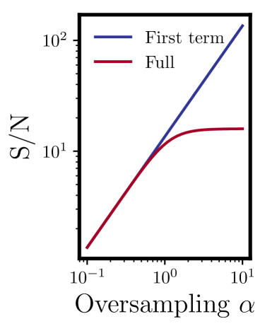
Note that for the case of well separated apertures, the cross-correlation coefficient will vanish and only the first summand needs to be taken into account, which for unity weights gives the familiar $1/N_{\rm ap}$ scaling of the variance. If the apertures are oversampled, this assumption is no longer valid and the term involving $\rho$ must be included. Owing to the fact that $\rho$ should only depend on the relative spatial distance $\Delta$ between the aperture centres, we can rewrite (3.4) as a weighted sum over all possible distances between aperture center pairs:

$$\sigma^{2}\left[\hat{\mathfrak{M}}\right]=\ S_{2}\ \sigma^{2}\left[{\hat{\mathfrak{M}}_{\rm{ap}}}\right]+$$

$$\frac{\sigma^{2}\left[{\hat{\mathfrak{M}}_{\rm{ap}}}\right]}{\left(\sum_{i}w_{i}\right)^{2}}\sum_{b\in\rm bins}\left(\sum_{i,j\in\mathcal{I}_{b}}w_{i}w_{j}\right)\rho(\hat{\mathfrak{M}},\Delta_{b})$$ (40)

$$\approx \frac{\sigma^{2}\left[{\hat{\mathfrak{M}}}_{\mathrm{ap}}\right]}{N_{\mathrm{ap}}}+2\pi\ \frac{\sigma^{2}\left[{\hat{\mathfrak{M}}}_{\mathrm{ap}}\right]}{A_{\mathrm{survey}}}\int_{R_{\mathrm{ap}}/\alpha}^{\infty}{\rm d}\Delta\ \Delta\ \rho(\hat{\mathfrak{M}},\Delta)\ ,$$ (41)

where in the first step the bins are defined as a partition of the reals, and $\mathcal{I}_{b}\equiv\{i,j|\Delta(i,j)\in b\}$ collects all the aperture center pairs falling into bin $b$. For the second step we make the approximation that each aperture contains roughly the same signal such that the weights can be set to unity and we furthermore rewrote the expression in a continuous version, which makes the interpretation of the cross term more concise. In particular, we parametrize the lower bound of the integral in terms of the aperture oversampling rate $\alpha\equiv R_{\mathrm{ap}}/\Delta_{\mathrm{min}}$.

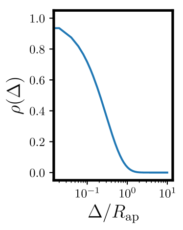
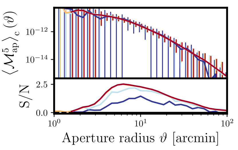
In a realistic scenario we expect $\rho$ to to rapidly decrease from unity and then to approach zero for $\Delta\gg R_{\mathrm{ap}}$. An example of such a correlation coefficient is shown in Fig. 1. Here we explicitly see the importance of taking into account the cross term once there is a substantial overlap between neighbouring apertures. In this example we would infer that measuring the statistics with $\alpha\approx 2$ would be sufficient to extract most of the signal.

3.5 Implementation and scaling of the direct estimator

A practical implementation of Eq. (34) consists of three steps:

1. Spatially organise the shape catalog to allow for a fast assignment of galaxies to apertures.

2. For each aperture of the ensemble compute $\hat{\mathfrak{M}}_{\rm ap}$, the associated weight and optionally additional systematics (i.e. the coverage fraction $c_{k}$). Store each of these values in an array.

3. Based on some aperture selection and aperture weighting criteria $w_{\rm ap}$, update the weights and evaluate the weighted sum.

In what follows we will explore each of these steps in more detail and for clarity we will denote the number of galaxies in the survey and in the aperture as $N_{\rm g}$ and $N_{\rm g,ap}$, respectively.

3.5.1 Assigning galaxies to apertures

For our implementation we use a spatial hashing data structure. We start by covering the survey footprint with an equal area mesh of $N_{\rm pix}$ pixels and create a hash table with the ID of each pixel as the key and the galaxy IDs as values. The hash function in our case is the ordinary pixel assignment function. For each aperture we iterate over the associated galaxies within pixels that partially lie within the $Q$ filter’s support. The construction of the hash table scales as $\mathcal{O}\left(\max(N_{\rm pix},N_{\rm g})\right)$ and the assignment is achieved in $\mathcal{O}\left(\max(N_{\rm pix,ap},N_{\rm g,ap})\right)$ time per aperture. We found that when making a sensible choice of the mesh’s coarseness, this data structure is more stable than a naive KD-tree based implementation as it does not require an additional range search operation which scales as $\mathcal{O}(\log(N_{\rm g}))$ per aperture and thus becomes a bottleneck for small apertures.

Figure 2: Computational complexity of the direct estimators for equal (left) and unequal (right) aperture radii as a function of the number of galaxies. All results are given for apertures of radius $10^{\prime}$ which are oversampled by a factor of sixteen $(\alpha=4)$ on a survey field of size $(12\rm{deg})^{2}$. Different colors indicate different orders of the evaluated statistics. The black dashed line indicates the time spent in constructing the spatial hash. We see that for equal aperture radii the evaluation of higher order statistics basically comes for free, while for unequal radii there is a constant multiplicative offset based on the relative size of the radii and on the order which traces the number of multivariate power sums that need to be evaluated. All the scaling were obtained when running the estimator on a single CPU core.

3.5.2 Computing the statistics per aperture

For the case of all radii being equal we first compute the power sums in Eqs (22) and (23) and then recursively transform them to the corresponding moments via the recurrence relation (Comtet, 1974)

$$B_{n+1}(x_{1},\cdots,x_{n+1}) =\sum_{i=0}^{n}\binom{n}{i}B_{n}(x_{1},\cdots,x_{n})x_{i+1}\ ,$$ (42)

where $B_{0}\equiv 1$. Evaluating each power sum is linear in $N_{\rm g,ap}$ and for all practical applications the time taken for transforming to the $M_{\rm ap}^{n}$ basis can be neglected.

For the general case we need to compute the relevant multivariable power sums Eq. (3.2) and bring them to the aperture moments basis by the transformation Eq. (3.2). In order to dynamically allocate and evaluate those expressions we use a combinadic counting scheme to organize the power sum basis whereas the transformation equation is generated with the help of restricted growth strings (Knuth, 2005).

3.5.3 Choice of weights for the averaging

Following our findings in Porth et al. (2020) we employ an inverse shot noise weighting scheme with an additional hard cutoff $c_{\rm lim}$ for the aperture coverage $c_{\rm ap}$, which for second order statistics was found to lower the mask induced bias while increasing the signal-to-noise compared to equal weights. The explicit form of the weights for the $n$th moment can be found from Eq. (37) when neglecting all constant contributions:

$$\mathcal{W}^{\rm(shot)}_{\rm ap}(c_{\rm lim})\equiv\left[\frac{\sum_{(i_{1},\cdots,i_{n})}w_{i_{1}}^{2}\cdots w_{i_{n}}^{2}}{\left(\sum_{(i_{1},\cdots,i_{n})}w_{i_{1}}\cdots w_{i_{n}}\right)^{2}}\right]^{-1}\mathcal{H}(c_{\rm ap}-c_{\rm lim})\ .$$ (43)

Dependent on whether we are dealing with the case of equal or unequal aperture radii the sums can be decomposed in a similar fashion as described above and evaluated together with the corresponding linearised direct estimator. As a further refinement one could also include the weights and completenesses of the surrounding apertures weighted by the spatial cross correlation coefficient $\hat{\rho}$ - this would upweight apertures that are close to a mask as they cover more unique area.

4 Results: application to Gaussian mocks

4.1 Aperture mass statistics and Gaussian lensing fields

Figure 3: Comparison of the measured aperture mass moments with their theoretical prediction. Left panel: The upper subpanel shows the aperture mass dispersion as a function of the aperture scale. The red line shows the theoretical predictions evaluated from the input power spectrum and the blue line shows the measurement from the mocks. The blue shaded regions show the standard deviation of the corresponding measurement across the ensemble. The lower subpanel shows the relative error between the measurement and the theory, with the line styles as before. Right panel: Same as left panel, but for the kurtosis of aperture mass.

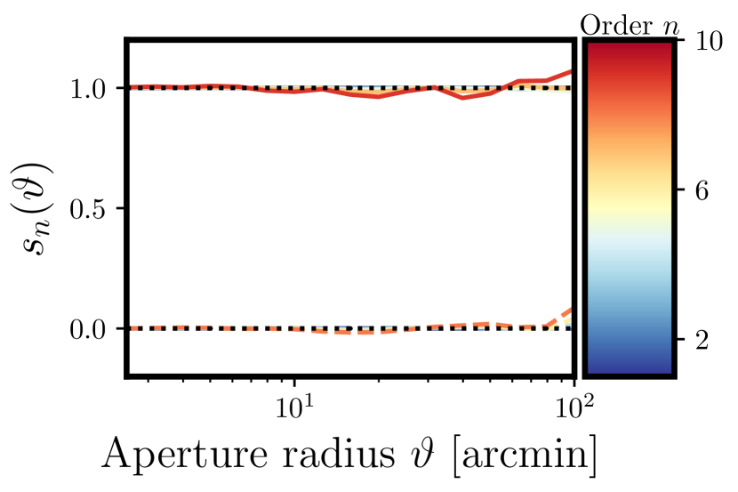
In order to validate that our hierarchy of aperture mass moment estimators are unbiased and do indeed recover correct results, we first apply them to a set of Gaussian mock lensing simulations. In this case, the whole moment hierarchy can be written as powers of the variance of the aperture mass. Hence, this motivates us to define the scaled aperture mass moments:

$$s_{n}(\vartheta_{1})\equiv\frac{1}{(n-1)!!}\frac{\left\langle\mathcal{M}_{\rm ap}^{n}\right\rangle(\vartheta_{1})}{\left[\left\langle\mathcal{M}_{\rm ap}^{2}\right\rangle(\vartheta_{1})\right]^{n/2}}=\delta^{K}_{n,2\mathbb{N}}\ ,$$ (44)

where the final equality is true for a Gaussian field only.

In order to test this we generated 256 Gaussian lensing mocks. The methodology to create each mock was as follows:

• We first generate a Gaussian convergence field over a $12\times 12\ {\rm square\ deg}$ survey area. The area is tiled by a rectangular mesh of $8192^{2}$ pixels. The variance of the convergence is obtained through specifying the convergence power spectrum, and we do this for a source distribution similar to that for the CFHTLenS survey (Fu et al., 2014).

• We next obtain the shear field. This is done by Fourier transforming the convergence field and making use of the Kaiser & Squires (1993) approach.

• We then sample $4\times 10^{6}$ galaxies into the survey footprint and use a multilinear interpolation of the shear field onto each galaxy.

Note that since we are assessing the accuracy of the estimators only we choose to set the intrinsic ellipticities of our source galaxies to zero. On repeating the analysis below when including this term we did not find a shift of the curves.

4.2 Computational scaling tests

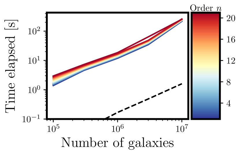
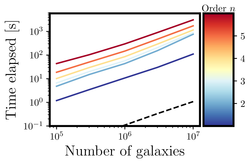
Owing to the fact that each step of our algorithm is strictly linear, we expect a linear relationship between the elapsed time for estimator evaluation and the number of galaxies, for any given statistic. In addition, for the equal radius case the order of the statistics should not strongly impact the evaluation time. However, for the unequal radius case, this does not necessarily hold true, since the computation depends on the relative sizes of the apertures as well as on the order of the statistics to be evaluated.

Figure  2 shows the elapsed time of the direct estimator calculation for a Gaussian mock, where the number of sampled galaxies in the mock is increased. Focusing on the left panel first, this shows the case for the standard aperture mass estimators with equal radii and here we compute all of the moments up to the 20th order. As expected the computational time for all of the moments scales linearly with the size of the problem and we also see that there is no obvious drop in performance for the higher order moments.

The right panel of Figure  2 is the same as the left panel, but now for the case of unequal radii aperture mass moments, and here we only consider moments up to 6th order. There are two differences between the equal and non-equal radius case. First, we can see that there is a much larger multiplicative offset between adjacent orders for the generalized statistics. This is expected as the number of basis elements that need to be allocated in that case is given by $2^{n}$ compared to the $n$ ones in the equal radius statistics. We also observe that for the second order statistic the unequal radius calculation does roughly need four times as long as the equal radius one. We can explain this offset when noting that for our example the ratio of the largest and smallest scale was set to two. With our definition of the oversampling rate as being relative to the smallest aperture radius this implies that we need to allocate four times as many galaxies.

Finally, we note that the superior scaling of the direct estimator compared to traditional estimation methods should not come as a surprise. Looking back at the original definition Eq. (2.2) of the aperture mass one sees that it depends on the positions and shapes of the galaxies with respect to the aperture origin. In contrast, when switching to the description of aperture mass in terms of the shear correlation functions (i.e. Schneider et al., 2002a), the main dependence shifts to the relative distance and shapes between tuples of galaxies. This change of reference position makes the evaluation of correlation function based estimators intrinsically much more complex than a simple discretization of Eq. (2.2).

Figure 4: Scaled $n$th order aperture mass moments $s_{n}(\vartheta)$ (see Eq. 44), measured in the ensemble of 256 Gaussian mocks, as a function of the aperture scale, for all moments up to 10th order. The solid lines of varying colours show the mean of the measurements. The dotted black lines show the Gaussian theoretical expectations. For a Gaussian mock, the even order $s_{n}(\vartheta)$ give unity, and the odd ones vanish.

Figure 5: Multiscale aperture mass moments as a function of the scale parameter $\vartheta$, measured in the ensemble of 256 Gaussian mocks. Line styles are the same as in Fig. 3. Left panel: the fourth order aperture statistics. In this case, the vector of aperture scales was set to $\bm{\alpha}=(0.5,0.8,1.,2.)$. Right hand side: Same as left hand side, but this time for the sixth order statistic with the vector of aperture scales set to $\bm{\alpha}=(0.5,0.7,1.,1.1,1.5,2.)$.

4.3 A hierarchy of aperture mass moments

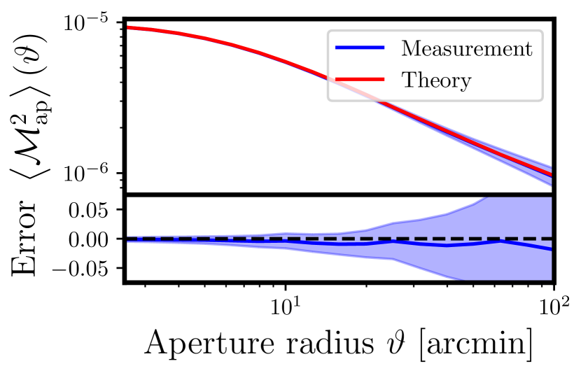
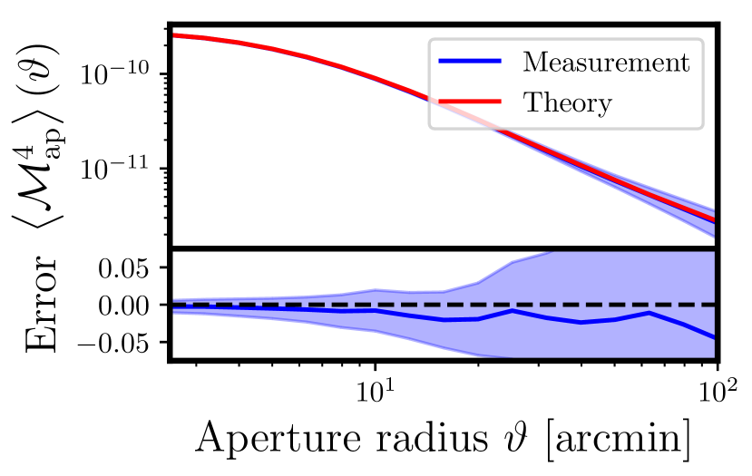
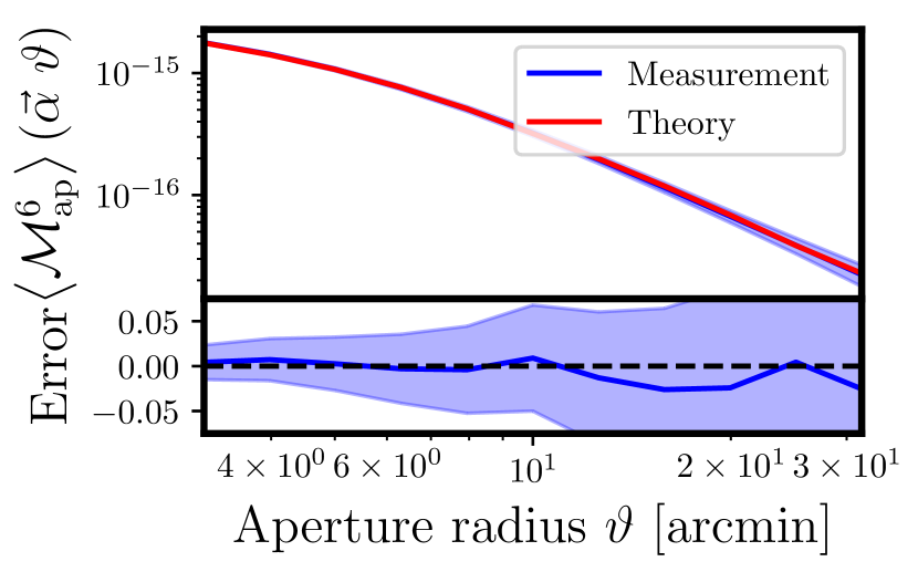
Figure  3 shows a comparison of the direct estimators for the second and fourth order aperture mass moments as a function of angular scale as applied to the 256 Gaussian mocks. Here we consider the case where all the aperture radii are equal (recall that for a Gaussian field all of the odd moments vanish). In both cases the curves are in very good agreement with the Gaussian theory predictions, indicated by the solid red lines. We also note that for increasingly large aperture radii the measured results appear to be slightly below the theoretical expectation. This discrepancy can be attributed to finite field effects, as well as border effects being introduced by the Kaiser-Squires inversion method (see Pires et al., 2020, for a discussion).

Figure  4 presents the measured $s_{n}$ (see Eq. (44)) for all of the aperture mass moments up to 10th order as a function of the aperture scale. We see that they are consistent with the Gaussian theoretical expectations. Note that in order to obtain this good agreement and circumvent the finite field effects described above, we used the ensemble mean of the measured aperture mass variance as the denominator in $s_{n}$.

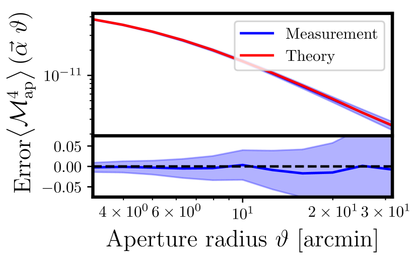
Figure  5 displays the fourth and sixth order multiscale aperture mass statistics as a function of the scale parameter. Note that there are a number of options for exploring the configuration dependence of the multiscale aperture mass moments, here we focus on fixing the ratio of the filter lengths and varying the overall scale of the configuration $\vec{a}$ with the parameter $\vartheta$, e.g. for the kurtosis we would have

$$\left\langle\mathcal{M}_{\rm ap}^{4}\right\rangle_{\rm c}(\vec{\vartheta})\equiv\left\langle\mathcal{M}_{\rm ap}^{4}\right\rangle_{\rm c}(a_{1}\vartheta,\cdots,a_{4}\vartheta)\$$ (45)

where the constant $a_{i}\in\mathbb{R}_{+}$ specify the configuration. The estimates shown in the figure were obtained using our generalized estimator Eq. (3.2). As for the previous cases, we find good agreement between the measurements and the Gaussian predictions, which were obtained by making use of Eq. (2.3) and Wicks theorem for the convergence polyspectra (Bernardeau et al., 2002).

Figure 6: Measurement of the aperture mass statistics in the SLICS simulation suite for different aperture oversampling rates $\alpha$. All measurements were done on an ensemble of 819 realizations with an angular area of 100 deg² each, where the $n(z)$ follows the KiDS-450 distribution. The upper part of the panels correspond to the mean and rescaled standard deviation from the ensembles. The lower panel shows the signal-to-noise for the corresponding statistics when rescaled to match a 1000 deg² survey. For the aperture mass dispersion we additionally plot the theoretical prediction as the black line. For the fourth and fifth order plots we restrict ourselves to the contribution of the connected part of the convergence polyspectra. We see that choosing an oversampling parameter of $\alpha\gtrsim 4$ recovers most of the information.

5 Results: Detection significance of higher order moments

In this section we now turn to the question of the detection significance of higher order aperture statistics from current and future surveys.

Figure 7: Correlation coefficient matrix (left) and cumulative detection significance (right) for connected moments of the aperture mass statistics. We take into account aperture sizes between $10^{\prime}$ and $100^{\prime}$. In the correlation matrix the lower triangle shows the results without shape noise while the upper part includes this term and serves as the basis for the computation of the detection significance.

Figure 8: Measurements of the unequal radii aperture mass statistics of third (left) and fifth (right) order in the SLICS simulation suite. Each line corresponds to a different set of relative aperture sizes as given in Table 1.

Figure 9: Measurements (left) and correlation matrix (right) of the multiscale aperture mass statistics of second, third and fourth order. For each of those statistics we compute all configurations for ten logarithmically spaced radii between $5^{\prime}$ and $50^{\prime}$ in which all the apertures have unequal radii. The black lines indicate the blocks of the (cross-) correlations of different orders.

Figure 10: Path in which the set of non redundant aperture scales for the third order statistics is traversed. The starting point is the lower corner. The subpath in the $\vartheta_{3}=50^{\prime}$ plane corresponds to the full path taken for the second order statistics.

5.1 The SLICS mocks

In order to answer this question we make use of the SLICS mocks – this is a large suite of lensing mock catalogues generated from a large set of cosmological $N$-body simulations (for full details see Harnois-Déraps et al., 2018). Each SLICS mock corresponds to a survey area of $100\deg^{2}$. These are generated from the past light cone extracted from fully independent gravity-only $N$-body simulations, which evolve $N=1532^{3}$ particles within a comoving box of length $L=505\,\,h^{-1}{\rm Mpc}$. The lensing maps are constructed using the Born approximation. We adopt the catalogues for which the galaxies are randomly distributed within the lightcone according to the KiDS-450 source distribution (Hildebrandt et al., 2017). The shape noise has been set to $\sigma_{\epsilon}=0.29$ per shear component. In order to mimic a constraining power that is comparable to the KiDS-1000 data while not being too noisy, we rescale the errorbars by a factor of $\sqrt{10}$. This provides us with effectively $819$ simulated $1000({\rm deg})^{2}$ surveys with which to perform our analysis.

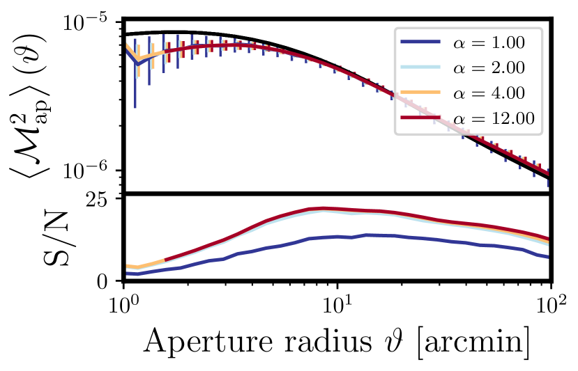
When estimating the aperture mass statistics from the SLICS mocks using the estimator given by Eq. (34), the achievable signal-to-noise ratio will depend on the number of sampled apertures selected. If too few are chosen then our estimate will be inefficient, on the other hand due to the fact that there are aperture-to-aperture correlations choosing too many will capture all of the available information, but ultimately will be computationally inefficient. We therefore expect that the information will saturate for a given oversampling rate, and that to sample at a higher rate would be of little use. To investigate this we proceed as in Porth et al. (2020) and place apertures on a regular grid with spacing $\Delta$, corresponding to an aperture oversampling rate of $\alpha\equiv\min\left(\{\vartheta_{i}\}\right)/2\Delta$.

5.2 Measurement in the SLICS mocks

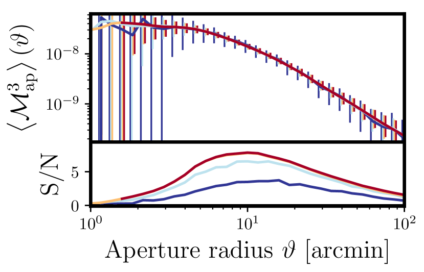
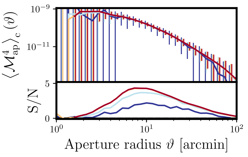
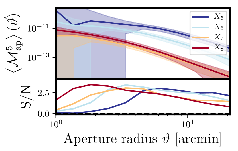
Figure  6 shows the detection significance of the equal radii aperture mass statistics for the second, third, fourth and fifth order aperture mass statistics as a function of the aperture scale and for various choices of the oversampling rate. For the second order statistics we also plot the theoretical prediction of the aperture mass dispersion evaluated from Eq. (2.2), where the convergence power spectrum was computed with CCL (Chisari et al., 2019) using Halofit (Smith et al., 2003), but with the modifications of Takahashi et al. (2012), as the matter power spectrum. While part of the difference between the curves for small aperture radii could be attributed to uncertainties in Halofit, our suspicion is that they mostly stem from the limited particle mass resolution in the SLICS mocks (see Fig. 6 in Harnois-Déraps et al. (2018) for the resulting suppression of the shear correlation functions for small separations).

Several important points are worth noting from these measurements. First, we see that for a KiDS-1000 like survey there is sufficient fidelity to detect the aperture mass statistics up to fourth order, with the signal-to-noise peaking at an aperture size of around $\vartheta\approx 10^{\prime}$ for all statistics. This is exciting, as this has never before been achieved with standard correlation function based estimators, and if correct would represent the first robust detection of these statistics using these methods. Second, while for the case of the two-point statistics the signal-to-noise ratio (shown in lower sub-panels for each plot) falls off slowly for larger apertures, this ratio approaches zero faster for the connected parts of the higher order statistics. Third, while an aperture oversampling rate of $\alpha\approx 2$ seems sufficient to capture all the signal for second order statistics, it misses some information for subsequent orders where it becomes necessary to use $\alpha\gtrsim 4$.

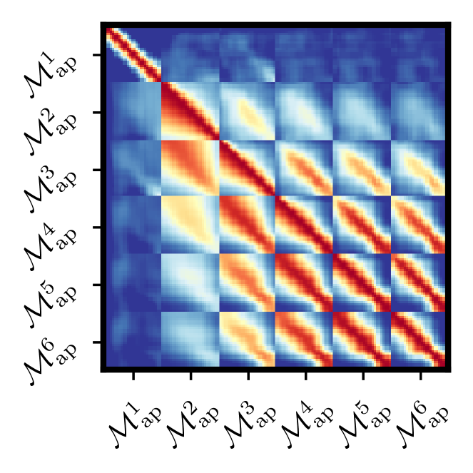
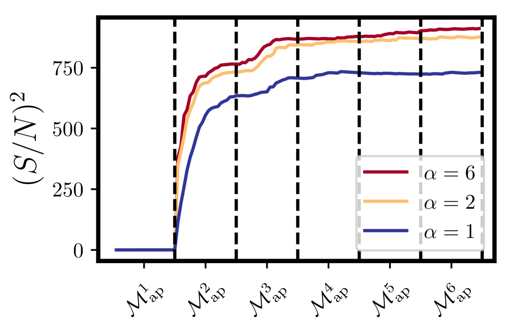
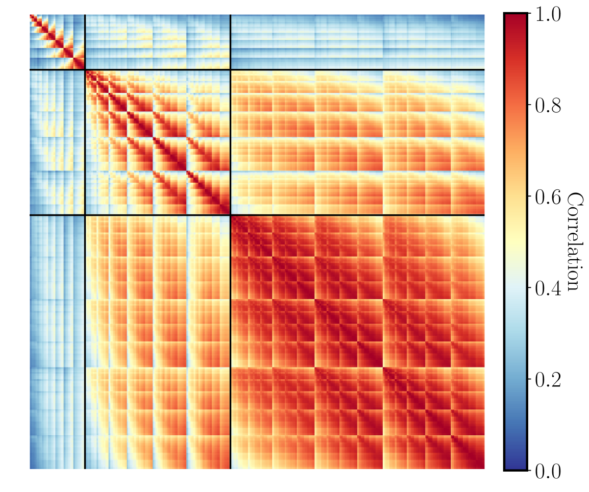
Figure  7 displays the correlation structure of the aperture mass cumulants as well as the cumulative detection significance. We only consider measurements with $\vartheta\geq 10^{\prime}$ as this is where the SLICS mocks do agree reasonably well with the theoretical predictions and and due to the fact that the robust theoretical modelling of those statistics might reach its limits at around those scales. We see that while for shape noise free ellipticity catalogs there are strong correlations for small aperture radii, this is not the case for the realistic mocks in which those scales are still shape noise dominated. We further note large correlations around the diagonal between different orders, where the degree of correlation increases with the order of the cumulants. For the cumulative detection significance we see that that the cumulants beyond third order do not add a substantial amplitude to the cumulative signal-to-noise. This is expected, given the relatively lower signal-to-noise as well as the larger portion of cross-covariances that need to be taken into account. One should note that this type of analysis does not imply that the higher order cumulants are obsolete as they still may add complementary information by breaking cosmological parameter degeneracies.

5.3 Multiscale aperture mass measurements

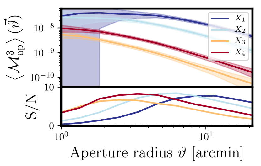
We now shift to the measurement of the multiscale statistics for which there are a number of ways on how to select various aperture scale multiplets. In Figure  8 we focus on a fixed set of aperture propositions and then simply scale them with a single parameter $\vartheta$. The different configurations $\vec{a}$ of aperture radii that we have employed are shown in Table 1. We see that for both, the third and the fifth order moments there does not appear to be a strong decline in detection significance for multiscale apertures compared to the associated moments, even if the relative spread of radii is large.

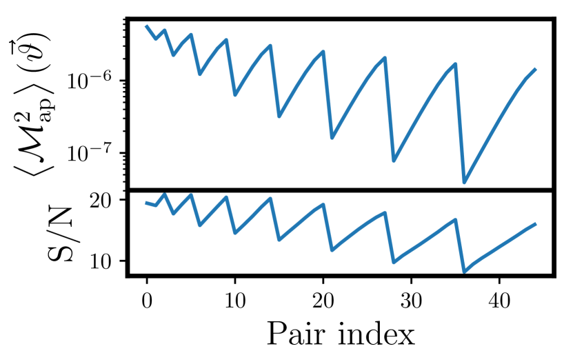
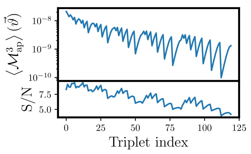
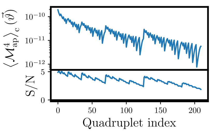
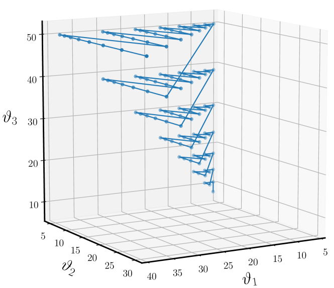
Another way to select aperture scale multiplets for a statistic of order $n$ is choose a list of $m\geq n$ aperture scales and to compute the statistics for each choice of $n$ elements within that list. For our purposes we choose the subset in which none of the aperture radii are equal, as this speeds up our calculation, see Appendix B.3 for the details. In the left hand side of Fig. 9 we show our measurements for the second, third and fourth order connected cumulants of the multiscale aperture mass statistic using ten logarithmically spaced scales between $5^{\prime}$ and $50^{\prime}$. The first index of the multiplet corresponds to the selection of the smallest possible aperture scales from which we then start choosing the next lowest radius in the subsequent dimension up until we reach the combination of the largest possible set of aperture radii - for an example of this path for the third order statistics see Fig. 10. Recalling that the second order aperture mass statistic is simply a filtered version of the power spectrum, we should not expect the multiscale extension add any information to that order. For the three statistics we again find a detection significance that is comparable to the equal scale case, meaning that we can extract substantial signal from convergence spectra configurations which are not corresponding to regular polygons. In the right hand side of Fig. 9 we plot the joint correlation coefficient of the multiscale cumulants. On the investigated range of scales we only find a slight to modest correlation between the higher order multiscale statistics and the second order one. It also appears that the higher order cumulants exhibit a stronger auto- and cross correlation. However, this is (at least partially) an artefact of the range and sampling density of the chosen radii.

Third order		Fifth order
Label	Configuration $\vec{a}$	Label	Configuration $\vec{a}$
$X_{1}$	$(1,1,1)$	$X_{5}$	$(1,1,1,1,1)$
$X_{2}$	$(1,2,2)$	$X_{6}$	$(1,1,2,2,2)$
$X_{3}$	$(1,5,5)$	$X_{7}$	$(1,1,5,5,5)$
$X_{4}$	$(1,3,5)$	$X_{8}$	$(1,2,3,4,5)$

Table 1: Cofigurations of the aperture radii displayed in Fig. 8

6 Conclusions and Discussion

In this paper we have explored an alternative method for estimating the aperture mass statistics in weak lensing cosmic shear surveys. This study extended our previous work (Porth et al., 2020) in a number of ways: First, we generalized the direct estimator approach to higher statistics, and showed how to rewrite the standard estimator as a product of linear order time sums. Second, we provided the details of the computation of the variance of these estimators. Third, we further generalised the aperture mass statistics to include the multiscale approach. Again, we showed how one could estimate these using linear order products of power sums. The work can be summarised as follows:

In §2 we reviewed the background theory of cosmological weak lensing and showed how the connected cumulants of the aperture mass statistics are related to the convergence polyspectra.

In §3 we introduced the direct estimator for moments of the aperture mass statistics. We then gave expressions for how the nested sums can be decomposed into a linear combination of products of (multivariate) power sums that facilitates a linearly scaling estimation procedure in the number of galaxies within an aperture. We then generalized this estimator to an ensemble of overlapping apertures and computed its variance. We argued that the aperture cross correlation coefficient leads to a substantial correction to the naive $1/N$ scaling if the apertures are not well separated, and that it also can be used to assess the degree of aperture oversampling that is necessary to capture most of the available information. Finally, we gave a detailed explanation of the algorithms used for our implementation.

In §4 we successfully validated our method on Gaussian mock simulations and furthermore verified the linear scaling.

In §5 we turned to the SLICS simulation suite and assessed the signal-to-noise of the statistics for a $1000$ degree survey following a KiDS-450 like $n(z)$ distribution function. We found that with these specifications significant detections of up to fourth order can be expected for the equal and unequal radii cumulants and that an aperture oversampling rate of at least four extracts nearly all the signal.

In this paper we have neglected the impact of survey masks on the measurement process and the possible bias that this could induce, the exploration of this is sufficient to warrant its own publication and this is the subject of our associated publication (Porth et al. in prep.). Throughout this paper we were mainly concerned with making the extraction of information from higher order statistics of galaxy shape catalogs computationally feasible and accurate. However, we remained agnostic about further challenges that need to be addressed before applying our methods to real data. For example, one should investigate the required PSF modelling, shape measurement and shear bias calibration quality to not introduce substantial biases in the measurement. Additionally, the range of measurements that can ultimately be used for obtaining cosmological parameter constraints will be limited to the scales for which one can theoretically accurately model those higher order statistics.

Data Availability

The SLICS mock catalogs are available at https://slics.roe.ac.uk/. Additional data underlying this article will be shared on reasonable request to the corresponding author.

Appendix A Derivations of aperture mass skewness and kurtosis estimators

In the following we will derive the accelerated direct estimators for the third and fourth order aperture mass moments. For properly treating summation indices we add to our notation (17) the following generalizations that deal with individual indices being set equal with each other:

$$\sum_{\begin{subarray}{c}{i_{1},\cdots,i_{l}\cdots i_{m-1},i_{m+1},\cdots,i_{n}}\\ {i_{l}=i_{m}}\end{subarray}} \equiv\sum_{i_{1}}\cdots\sum_{i_{m-1}}\sum_{i_{m+1}}\cdots\sum_{i_{n}}$$ (46)

$$\sum_{\begin{subarray}{c}({i_{1},\cdots,i_{l}\cdots i_{m-1},i_{m+1}\cdots i_{n}})\\ {i_{l}=i_{m}}\end{subarray}} \equiv\sum_{i_{1}}\sum_{i_{2}\neq i_{1}}\cdots\sum_{i_{m-1}\neq\cdots\neq i_{1}}\sum_{i_{m+1}\neq\cdots\neq i_{1}}\cdots\sum_{i_{n}\neq\cdots\neq i_{1}}$$ (47)

A.1 Derivation of the estimator for $\widehat{M_{\rm ap}^{3}}$

Let us compute the derivation of the skewness $\widehat{M_{\rm ap}^{3}}$ of the aperture mass. The standard direct estimator is given by:

$$\widehat{M_{\rm ap}^{3}}=(\pi\vartheta^{2})^{3}\frac{\sum_{(i,j,k)}^{N}w_{i}w_{j}w_{k}Q_{i}Q_{j}Q_{k}e_{t,i}e_{t,j}e_{t,k}}{\sum_{(i,j,k)}^{N}w_{i}w_{j}w_{k}}\ .$$ (48)

It can be shown using the methods described in Schneider et al. (1998) and Porth et al. (2020) that this leads to an unbiased estimator of the skewness. We can rewrite the above estimator by noting that an unconstrained triple sum can be decomposed into the following partial sums:

$$\sum_{i,j,k}^{N} =\sum_{(i,j,k)}^{N}+\sum_{\begin{subarray}{c}({i,j})\\ {i=k}\end{subarray}}^{N}+\sum_{\begin{subarray}{c}({i,j})\\ {j=k}\end{subarray}}^{N}+\sum_{\begin{subarray}{c}({i,k})\\ {i=j}\end{subarray}}^{N}+\sum_{i=j=k}^{N}$$ (49)

This can be rearranged to give:

$$\sum_{(i,j,k)}^{N} =\sum_{i,j,k}^{N}-\sum_{\begin{subarray}{c}({i,j})\\ {i=k}\end{subarray}}^{N}-\sum_{\begin{subarray}{c}({i,j})\\ {j=k}\end{subarray}}^{N}-\sum_{\begin{subarray}{c}({i,k})\\ {i=j}\end{subarray}}^{N}-\sum_{i=j=k}^{N}$$ (50)

Similarly, the unconstrained double sum can be decomposed and rearranged in the following manner:

$$\sum_{i,j}=\sum_{(i,j)}+\sum_{i=j}\ \ \Rightarrow\ \ \sum_{(i,j)}=\sum_{i,j}-\sum_{i=j}\ .$$ (51)

Using this result repeatedly in Eq. (50) allows us to rewrite the constrained sums as unconstrained sums:

$$\sum_{(i,j,k)}^{N} =\sum_{i,j,k}^{N}-\left(\sum_{\begin{subarray}{c}{i,j}\\ {i=k}\end{subarray}}^{N}-\sum_{i=j=k}^{N}\right)-\left(\sum_{\begin{subarray}{c}{i,j}\\ {j=k}\end{subarray}}^{N}-\sum_{i=j=k}^{N}\right)-\left(\sum_{\begin{subarray}{c}{i,k}\\ {i=j}\end{subarray}}^{N}-\sum_{i=j=k}^{N}\right)-\sum_{i=j=k}^{N}$$

$$=\sum_{i,j,k}^{N}-\sum_{\begin{subarray}{c}{i,j}\\ {i=k}\end{subarray}}^{N}-\sum_{\begin{subarray}{c}{i,j}\\ {j=k}\end{subarray}}^{N}-\sum_{\begin{subarray}{c}{i,k}\\ {i=j}\end{subarray}}^{N}+2\sum_{i=j=k}^{N}\ =\sum_{i,j,k}^{N}\left[1-\delta^{K}_{j,k}-\delta^{K}_{k,i}-\delta^{K}_{i,j}+2\delta^{K}_{i,j}\delta^{K}_{i,k}\right]\ .$$ (52)

Hence, on repeatedly using this result we can rewrite the sum in the numerator and denominator of Eq. (48) to give us an alternate form for the skewness as:

$$\widehat{M_{\rm ap}^{3}}=(\pi\vartheta^{2})^{3}\frac{\left[\sum_{i,j,k}^{N}w_{i}w_{j}w_{k}Q_{i}Q_{j}Q_{k}e_{t,i}e_{t,j}e_{t,k}-3\sum_{i,j}^{N}w_{i}w_{j}^{2}Q_{i}Q_{j}^{2}e_{t,i}e_{t,j}^{2}+2\sum_{i}^{N}w_{i}^{3}Q^{3}_{i}e^{3}_{t,i}\right]}{\left[\sum_{i,j,k}^{N}w_{i}w_{j}w_{k}-3\sum_{i,j}^{N}w_{i}w_{j}^{2}+2\sum_{i}^{N}w_{i}^{3}\right]}\ .$$ (53)

If we now divide through each term by $(\sum_{i}^{N}w_{i})^{3}$ and recall expressions Eqs (22) and (23) we see that our estimator becomes:

$$\widehat{M_{\rm ap}^{3}} =\frac{M_{{\rm s},1}^{3}-3M_{{\rm s},2}M_{{\rm s},1}+2M_{{\rm s},3}}{1-3S_{2}+2S_{3}}\ .$$ (54)

A.2 Derivation of the estimator for $\widehat{M_{\rm ap}^{4}}$

The standard direct estimator for the kurtosis of aperture mass is given by:

$$\widehat{M_{\rm ap}^{4}}=(\pi\vartheta^{2})^{4}\frac{\sum_{(i,j,k,l)}^{N}w_{i}w_{j}w_{k}w_{l}Q_{i}Q_{j}Q_{k}Q_{l}e_{t,i}e_{t,j}e_{t,k}e_{t,l}}{\sum_{(i,j,k,l)}^{N}w_{i}w_{j}w_{k}w_{l}}\ .$$ (55)

We follow similar steps to the derivation of the skewness and note that the unconstrained quadruple sum can be written:

$$\sum_{i,j,k,l}^{N}= \sum_{(i,j,k,l)}^{N}+\left[\sum_{\begin{subarray}{c}({i,j,k})\\ {i=l}\end{subarray}}^{N}+\ 5\ {\rm perms}\right]+\left[\sum_{\begin{subarray}{c}({i,j})\\ {i=k,j=l}\end{subarray}}^{N}+\sum_{\begin{subarray}{c}({i,j})\\ {i=l,j=k}\end{subarray}}^{N}+\sum_{\begin{subarray}{c}({i,k})\\ {i=j,k=l}\end{subarray}}^{N}\right]+\left[\sum_{\begin{subarray}{c}({i,j})\\ {j=k=l}\end{subarray}}^{N}+\sum_{\begin{subarray}{c}({i,l})\\ {i=j=k}\end{subarray}}^{N}+\sum_{\begin{subarray}{c}({i,k})\\ {i=j=l}\end{subarray}}^{N}+\sum_{\begin{subarray}{c}({i,j})\\ {i=k=l}\end{subarray}}^{N}\right]+\sum_{i=j=k=l}^{N}\ ,$$ (56)

which on rearranging leads us to:

$$\sum_{(i,j,k,l)}^{N}= \sum_{i,j,k,l}^{N}-\left[\sum_{\begin{subarray}{c}({i,j,k})\\ {i=l}\end{subarray}}^{N}+\ 5\ {\rm perms}\right]-\left[\sum_{\begin{subarray}{c}({i,j})\\ {i=k,j=l}\end{subarray}}^{N}+\sum_{\begin{subarray}{c}({i,j})\\ {i=l,j=k}\end{subarray}}^{N}+\sum_{\begin{subarray}{c}({i,k})\\ {i=j,k=l}\end{subarray}}^{N}\right]-\left[\sum_{\begin{subarray}{c}({i,j})\\ {j=k=l}\end{subarray}}^{N}+\sum_{\begin{subarray}{c}({i,l})\\ {i=j=k}\end{subarray}}^{N}+\sum_{\begin{subarray}{c}({i,k})\\ {i=j=l}\end{subarray}}^{N}+\sum_{\begin{subarray}{c}({i,j})\\ {i=k=l}\end{subarray}}^{N}\right]-\sum_{i=j=k=l}^{N}\ .$$ (57)

We now make use of our previous results to rewrite the constrained sums on the right-hand side of the expression as unconstrained sums:

$$\sum_{(i,j,k,l)}^{N} =\sum_{i,j,k,l}^{N}-\left\{\left[\sum_{\begin{subarray}{c}{i,j,k}\\ {i=l}\end{subarray}}^{N}-\sum_{\begin{subarray}{c}{i,j}\\ {i=k=l}\end{subarray}}^{N}-\sum_{\begin{subarray}{c}{i,j}\\ {j=k,i=l}\end{subarray}}^{N}-\sum_{\begin{subarray}{c}{i,k}\\ {i=j=l}\end{subarray}}^{N}+\ 2\sum_{i=j=k=l}^{N}\right]+\ 5\ {\rm perms}\right\}-\left\{\left[\sum_{\begin{subarray}{c}{i,j}\\ {i=k,j=l}\end{subarray}}^{N}-\sum_{i=j=k=l}^{N}\right]+\left[\sum_{\begin{subarray}{c}{i,j}\\ {i=l,j=k}\end{subarray}}^{N}-\sum_{i=j=k=l}^{N}\right]\right.$$

$$+\left.\left[\sum_{\begin{subarray}{c}{i,k}\\ {i=j,k=l}\end{subarray}}^{N}-\sum_{i=j=k=l}^{N}\right]\right\}-\left\{\left[\sum_{\begin{subarray}{c}{i,j}\\ {j=k=l}\end{subarray}}^{N}-\sum_{i=j=k=l}^{N}\right]+\left[\sum_{\begin{subarray}{c}{i,l}\\ {i=j=k}\end{subarray}}^{N}-\sum_{i=j=k=l}^{N}\right]+\left[\sum_{\begin{subarray}{c}{i,k}\\ {i=j=l}\end{subarray}}^{N}-\sum_{i=j=k=l}^{N}\right]+\left[\sum_{\begin{subarray}{c}{i,j}\\ {i=k=l}\end{subarray}}^{N}-\sum_{i=j=k=l}^{N}\right]\right\}-\sum_{i=j=k=l}^{N}\ .$$ (58)

On making repeated use of the Kroneker delta symbol this can now be compactly written as:

$$\sum_{(i,j,k,l)}^{N} =\sum_{i,j,k,l}^{N}\Bigg{[}1-\left\{\left[\delta^{K}_{k,l}-\delta^{K}_{j,k}\delta^{K}_{k,l}-\delta^{K}_{i,k}\delta^{K}_{k,l}-\delta^{K}_{i,j}\delta^{K}_{k,l}+2\delta^{K}_{i,j}\delta^{K}_{i,k}\delta^{K}_{i,l}\right]+5\ {\rm perms}\right\}-\Big{\{}\left[\delta^{K}_{i,j}\delta^{K}_{k,l}-\delta^{K}_{i,j}\delta^{K}_{i,k}\delta^{K}_{i,l}\right]$$

$$+\left[\delta^{K}_{i,k}\delta^{K}_{j,l}-\delta^{K}_{i,j}\delta^{K}_{i,k}\delta^{K}_{i,l}\right]+\left[\delta^{K}_{i,l}\delta^{K}_{j,k}-\delta^{K}_{i,j}\delta^{K}_{i,k}\delta^{K}_{i,l}\right]\Big{\}}-\Big{\{}\left[\delta^{K}_{i,j}\delta^{K}_{i,k}-\delta^{K}_{i,j}\delta^{K}_{i,k}\delta^{K}_{i,l}\right]$$

$$+\left[\delta^{K}_{i,j}\delta^{K}_{i,l}-\delta^{K}_{i,j}\delta^{K}_{i,k}\delta^{K}_{i,l}\right]+\left[\delta^{K}_{i,k}\delta^{K}_{i,l}-\delta^{K}_{i,j}\delta^{K}_{i,k}\delta^{K}_{i,l}\right]+\left[\delta^{K}_{j,k}\delta^{K}_{j,l}-\delta^{K}_{i,j}\delta^{K}_{i,k}\delta^{K}_{i,l}\right]\Big{\}}-\delta^{K}_{i,j}\delta^{K}_{i,k}\delta^{K}_{i,l}\Bigg{]}\ .$$ (59)

On collecting, cancelling and grouping like terms we see that this can be written:

$$\sum_{(i,j,k,l)}^{N} =\sum_{i,j,k,l}^{N}\Bigg{[}1-\left(\delta^{K}_{i,j}+\delta^{K}_{i,k}+\delta^{K}_{i,l}+\delta^{K}_{j,k}+\delta^{K}_{j,l}+\delta^{K}_{k,l}\right)+\left\{\delta^{K}_{i,j}\delta^{K}_{k,l}+\delta^{K}_{i,k}\delta^{K}_{j,l}+\delta^{K}_{i,l}\delta^{K}_{j,k}\right\}$$

$$+\left\{\delta^{K}_{i,j}\delta^{K}_{i,k}+\delta^{K}_{i,j}\delta^{K}_{i,l}+\delta^{K}_{i,k}\delta^{K}_{i,l}+\delta^{K}_{j,i}\delta^{K}_{j,k}+\delta^{K}_{j,i}\delta^{K}_{j,l}+\delta^{K}_{j,k}\delta^{K}_{j,l}+\delta^{K}_{k,i}\delta^{K}_{k,l}+\delta^{K}_{k,j}\delta^{K}_{k,l}\right\}-6\delta^{K}_{i,j}\delta^{K}_{i,k}\delta^{K}_{i,l}\Bigg{]}\ .$$ (60)

Hence, on making repeated use of Eq. (60) in Eq. (55) and along with Eqs (22) and (23), the estimator for kurtosis of aperture mass becomes:

$$\widehat{M_{\rm ap}^{4}} =\frac{M_{{\rm s},1}^{4}-6M_{{\rm s},2}M_{{\rm s},1}^{2}+3M_{{\rm s},2}^{2}+8M_{{\rm s},3}M_{{\rm s},1}-6M_{{\rm s},4}}{1-6S_{2}+3S_{2}^{2}+8S_{3}-6S_{4}}\ .$$ (61)

Appendix B A proof of the general theorem for arbitrary order aperture mass statistics

In this section we provide a derivation of the the general form of the $n$-point aperture mass statistic estimator given by Eq. (24). At the time of writing, we are not aware that the combinatoric methods that we have used in the derivation of the general expression have been used before in the cosmological context, and therefore provide a brief overview of them – in particular the Bell polynomials. In what follows we will try to not rely on advanced mathematical methods, but instead use a basic framework to explain how the Bell polynomials are linked to set partitions, and finally how they are connected to the aperture mass estimators.

B.1 Set partitions and Bell polynomials

We begin by defining a partition $\pi$ of a set ${\bf n}=\{1,2,\cdots,n\}$ as a collection of mutually exclusive subsets (blocks) of ${\bf n}$ whose union equals ${\bf n}$. In our case all these partitions can be mapped onto an associated partition $\lambda$ being defined as the number of elements of each block in $\pi$. Each element $\lambda$ can be represented as $(n_{1},n_{2},\cdots,n_{m})$ or as $\left(1^{m_{1}},\ 2^{m_{2}},\ \cdots,n^{m_{n}}\right)$ where for the former expression the $n_{i}$ denote the length of the $i$th block while for the latter case the $m_{i}$ represent the number of occurrences of a block of length $i$ in $\pi$. If $\pi$ is a partition of ${\bf n}$ having $m$ blocks this implies that $\sum_{i}m_{i}=m$ and $\sum_{i}i\ m_{i}=n$. We will now show that the following proposition holds:

Proposition:
For the set ${\bf n}$ and a partition $\lambda$ of length $m$ given as $\left(1^{m_{1}},\ 2^{m_{2}},\ \cdots,\ell^{m_{\ell}}\right)$ there are $\frac{n!}{\prod_{i=1}^{\ell}m_{i}!(i!)^{m_{i}}}$ partitions $\pi$ of ${\bf n}$ having the same $\lambda(\pi)$.
Proof:
As a first step we just look at the number of ways the $m$ subsets can be chosen from $\bm{n}$. This can easily be worked out when noting that for the first subset there are $\binom{n}{n_{1}}$ choices, for the following $\binom{n-n_{1}}{n_{2}}$ etc. Following through all of the subsets we then have

$$\binom{n}{n_{1}}\binom{n-n_{1}}{n_{2}}\cdots\binom{n-n_{1}-\cdots n_{m-2}}{n_{m-1}}\binom{n_{m}}{n_{m}}=\frac{n!}{n_{1}!(n-n_{1})!}\frac{(n-n_{1})!}{n_{2}!(n-n_{1}-n_{2})!}\cdots\frac{(n-n_{1}-\cdots n_{m-2})!}{n_{m-1}!n_{m}!}\frac{n_{m}!}{n_{m}!}=\frac{n!}{n_{1}!n_{2}!\cdots n_{m}!}$$ (62)

possibilities. Shifting this expression to the representation of $\lambda$ given above we see that many of them give the identical partition $\pi$; to get rid of those ones we need to divide by the number of ways all the equal size blocks themselves can be permuted with each other. Applying those conditions we have

$$\frac{1}{\text{Norm.}}\times\frac{n!}{n_{1}!n_{2}!\cdots n_{m}!}=\frac{1}{m_{1}!m_{2}!\cdots m_{\ell}!}\times\frac{n!}{(1!)^{m_{1}}(2!)^{m_{2}}\cdots(\ell!)^{m_{\ell}}}=\frac{n!}{\prod_{i=1}^{\ell}m_{i}!(i!)^{m_{i}}}$$ (63)

possibilities remaining, which is exactly the proposed expression.

With this result in hand we are now in position to understand the form of the partial Bell polynomial $B_{n,m}$ being defined as

$$B_{n,m}(x_{1}\cdots,x_{n-m+1}) =\sum_{(m_{1},\cdots,m_{n-m+1})\in P_{n,m}}\frac{n!}{m_{1}!\cdots m_{n-m+1}!}\left(\frac{x_{1}}{1!}\right)^{m_{1}}\cdots\left(\frac{x_{n-m+1}}{(n-m+1)!}\right)^{m_{n-m+1}}\ \ ,$$ (64)

where

$$P_{n,m} \equiv\left\{(m_{1},\cdots m_{n-m+1})\ \in\ \mathbb{N}_{0}^{n-m+1}\ |\ \sum_{i=1}^{n-m+1}m_{i}=m\ \ ,\ \ \sum_{i=1}^{n-m+1}i\ m_{i}=n\right\}\ .$$

Comparing the prefactors and the index set with our discussion above we see that the partial Bell polynomials simply sum over all the partitions $\lambda$ of ${\bf n}$ having a fixed $m$, i.e. they list the number of ways a set consisting the $n$ objects can be partitioned into $m$ blocks. For example, looking at $B_{4,2}$ the allowed index combinations are $\{(0,2,0),(1,0,1)\}$ such that Eq. (64) evaluates to $B_{4,2}=4x_{1}x_{3}+3x_{2}^{2}$. We note in the passing that these expressions generate the same prefactors that arise in the halo model, i.e. we can relate the structure of $B_{4,2}$ to the two-halo term of the halo model trispectrum.

Finally, we define the complete Bell polynomial $B_{n}$ which list all possible partitions of $n$ objects:

$$B_{n}(x_{1}\cdots,x_{n-m+1}) =\sum_{m=1}^{n}B_{n,m}(x_{1}\cdots,x_{n-m+1})=\sum_{m=1}^{n}\sum_{\pi\in P_{n,m}}\prod_{i=1}^{n-m(\lambda(\pi))+1}x_{i}^{m_{i}(\lambda(\pi))}\ ,$$ (65)

where the first equality states the formal definition and the second one rewrites it into an explicit sum over all the partitions of the set $\bm{n}$.

B.2 Sums over unequal indices and Bell polynomials

Let us look at the simple expression $\sum_{i=1}^{N}\sum_{j\neq i}^{N}x_{i}x_{j}$. A naive implementation of this double sum would imply a quadratic complexity of the corresponding program. A much faster way resulting in linear complexity can be achieved when noting that $\left(\sum_{i_{1}=1}^{N}x_{i_{1}}\right)\left(\sum_{i_{2}=1}^{N}x_{i_{2}}\right)=\sum_{i_{1}=1}^{N}\sum_{i_{2}\neq i_{1}}^{N}x_{i_{1}}x_{i_{2}}+\sum_{i_{1}=1}^{N}x_{1}^{2}\$. We can easily generalize this pattern by treating the number of indices as the set ${\bf n}$ from the previous subsection. Then all the different partitions $\lambda$ of this set correspond to different ways these indices can be set equal with one another; the corresponding prefactors can be obtained via the Bell polynomial. To clarify this statement we write down as an example the expression for $n=4$:

$$\left(\sum_{i}x_{i}\right)^{4} =\sum_{i_{1}\neq i_{2}\neq i_{3}\neq i_{4}}x_{i_{1}}x_{i_{2}}x_{i_{3}}x_{i_{4}}\ +\ \left(\sum_{i_{1}\neq i_{3}\neq i_{4}}x_{i_{1}}^{2}x_{i_{3}}x_{i_{4}}+5\text{perm.}\right)\ +\ \left(\sum_{i_{1}\neq i_{2}}x_{i_{1}}^{3}x_{i_{2}}+3\text{perm.}\right)\ +\ \left(\sum_{i_{1}\neq i_{3}}x_{i_{1}}^{2}x_{i_{3}}^{2}+2\text{perm.}\right)\ +\ \sum_{i_{1}}x_{i_{1}}^{4}$$ (66)

$$\sim(1^{4},\ 2^{0}\ ,\ 3^{0}\ ,\ 4^{0})\ \ +\ \ 6\times(1^{2}\ ,\ 2^{1}\ ,\ 3^{0}\ ,\ 4^{0})\ \ +\ \ 4\times(1^{1}\ ,\ 2^{0}\ ,\ 3^{1}\ ,\ 4^{0})\ \ +\ \ 3\times(1^{0}\ ,\ 2^{2}\ ,\ 3^{0}\ ,\ 4^{0})\ \ +\ \ (1^{0}\ ,\ 2^{0}\ ,\ 3^{0}\ ,\ 4^{1})$$

From here we see that we can express a sum over $n$ unequal indices in terms of two power sums and a set of related sums over at most $n-1$ unequal indices. Repeating the same argument on the latter sums one eventually arrives at an expression only involving power sums. Carrying out aforementioned calculations along the lines of Appendix A for our example this yields

$$\sum_{i_{1}\neq i_{2}\neq i_{3}\neq i_{4}}x_{i_{1}}x_{i_{2}}x_{i_{3}}x_{i_{4}}=\left(\sum_{i}x_{i}\right)^{4}-6\left(\sum_{i}x_{i}\right)^{2}\left(\sum_{i}x_{i}^{2}\right)+\ 8\left(\sum_{i}x_{i}\right)\left(\sum_{i}x_{i}^{3}\right)+\ 3\left(\sum_{i}x_{i}^{2}\right)^{2}-\ 6\left(\sum_{i}x_{i}^{4}\right)\ \ .$$ (67)

Comparing the latter two expressions we note that their index partitions are the same, but that they differ in some signs and prefactors; namely there is a negative sign for an odd partition length $m$ and an additional multiplicative factor of $(i-1)!$ for each block of length $i$. Looking at the structure of Eq. (67), i.e. the fact that all of its summands correspond to a partition of an integer set and that furthermore it constitutes of $n$ different building blocks we might be tempted to cast it in terms of Bell polynomials with the identifying the $x_{\ell}$ from Eq. (65) with the power sums $c_{\ell}\sum_{i}x_{i}^{\ell}\ \ :\ \ c_{\ell}\in\mathbb{R}$. In the next paragraphs we formalize these observations and from there determine the $c_{\ell}$.

The first difference can be motivated most easily by choosing a graphical representation in which we draw each index as a single point. Then the prefactors in Eq. (66) are given by the number of ways one can group together different points such that they constitute the corresponding partition whereas for Eq. (67) it additionally matters in which order these points have been set equal with each other, which in mathematical terms is described by how many closed cycles one can draw between them. The induced correction of $(\ell-1)!$ for a block of length $\ell$ can be absorbed in the Bell polynomial by setting $c_{\ell}=(\ell-1)!$.

The second observation can be generalized inductively. Looking at our example of $n=4$ we see that the sign for each partition $\lambda$ is given by $\text{sgn}(\lambda)$ = $\prod_{i=1}^{n}(-1)^{m_{i}(\lambda)((i+1)\text{mod}2)}$, that is each block of even length contributes a negative sign. Performing the induction step we have

$$\sum_{i_{1}\neq\cdots i_{n}\neq i_{n+1}}x_{i_{1}}\cdots x_{i_{n+1}}=\left(\sum_{i_{n+1}}x_{i_{n+1}}\right)\left(\sum_{i_{1}\neq\cdots i_{3}\neq i_{n}}x_{i_{1}}\cdots x_{i_{n}}\right)-\left[\left(\sum_{i_{1}\neq\cdots i_{3}\neq i_{n}}x_{i_{1}}^{2}x_{i_{2}}\cdots x_{i_{n}}\right)+(n-1)\ \text{perm.}\right]\ .$$ (68)

Looking at the modification of the partitions, for the first term we have $m_{1}\rightarrow m_{1}+1$ for all $\lambda$ such that we would not have expected any sign flips. For the second term, we need to update the block in which the identical index sits, assuming it had length $k$ we have $m_{k}\rightarrow m_{k}-1$ and $m_{k+1}\rightarrow m_{k+1}+1$. In case of an even $k$ reducing its occurrence by one induces an additional sign flip whereas for odd $k$s we get a sign flip for the increase of $m_{k+1}$. Putting things together we conclude that we could predict the correct signs by examining the partition structures. Therefore, setting $c_{\ell}=(-1)^{(\ell+1)\ \text{mod}\ 2}(\ell-1)!$ in Eq. (65) will reproduce generalizations of $Eq.\,(\ref{eq:helperAppA1_2})$. We can brush this in a nicer shape by setting $c_{\ell}=-(\ell-1)!$ and furthermore multiplying $B_{n}$ by $(-1)^{n}$; this modification effectively just multiplies each term of the previous result by an even power of negative one.

With these two modifications in hand we can finally write down the main result of this subsection, namely the way on how to transform a sum over unequal indices into a sum over products of power sums:

$$\sum_{i_{1}\neq\cdots\neq i_{n}}x_{i_{1}}\cdots x_{i_{n}}=(-1)^{n}\ B_{n}\left(-0!\ \sum_{i}x_{i},\ -1!\ \sum_{i}x_{i}^{2},\cdots,\ -(n-1)!\ \sum_{i}x_{i}^{n}\right)$$ (69)

B.3 Application to the aperture mass estimator

Looking at the form of Eq. (69), the expression for the direct estimator of the aperture statistics with equal aperture radii Eq. (24) immediately follows when identifying the arguments in the nominator and denominator with the power sums $M_{{\rm s},m}$ and $S_{m}$ and cancelling the overall sign.

For the case of unequal aperture radii we still need to do a bit more work. Looking back to our previous example Eq. (66), having unequal aperture radii induces different values of the $Q$ filters such that the $x_{i}$ cannot be taken to be the same variable anymore. Hence we have to replace the prefactors in Eq. (66) by a sum over all the possible ways the different radii can be partitioned. The second set of prefactors that arises when going to Eq. (67) still applies in the case of unequal radii as it effectively corresponds to swapping two aperture radii in the corresponding multivariate power sum Eq. (3.2). Thus it seems appropriate to formulate the solution via summing over partitions, such that we can rewrite Eq. (3.2) as

$$\widehat{M_{\rm ap}^{n}}(\vartheta_{1},...,\vartheta_{n})=\frac{\sum_{m=1}^{n}\sum_{\pi\in P_{n,m}}(-1)^{m}\prod_{i=1}^{m}(n_{i}-1)!\ {M_{\rm s,({\mathscr{s}_{1}(\pi_{i}),\cdots,\mathscr{s}_{n}(\pi_{i})})}^{({n_{i}})}}}{\sum_{m=1}^{n}\sum_{\pi\in P_{n,m}}(-1)^{m}\prod_{i=1}^{m}(n_{i}-1)!\ {S_{({\mathscr{s}_{1}(\pi_{i}),\cdots,\mathscr{s}_{n}(\pi_{i})})}^{({n_{i}})}}}\ .$$ (70)

We note that from this formulation one can build an efficient way of computing Eq. (3.2) within the subset $\mathcal{U}$ of the datacube $[R_{1},\cdots R_{m}]^{n}\ \ (m\geq n)$ in which neither of the indices are equal: This is due to the fact that the number of power sums in which $1\leq i\leq n$ radii are selected is simply given by $\binom{m}{i}$ and therefore the n-dimensional hypercube of aperture radii can be constructed from a set consisting of just $\sum_{i=1}^{n}\binom{m}{i}$ power sums. After allocating those power sums for all the galaxies within an aperture we can then enumerate through the relevant aperture radii multiplets, select the relevant subsets of the power sums, and then again apply the transformation equation (3.2) to transform to the multiscale aperture mass moments, or equivalently to their corresponding connected parts. With the help of this procedure we were able to conduct the full analysis displayed in Fig. 9 on the SLICS ensemble (a total of around 2.5 billion galaxies) within just $6000$ CPU hours.

B.4 Expressions of the accelerated estimator for low orders (unequal radii)

In order to save space we only write down the expressions for the nominator or Eq. (3.2), the denominator will have an identical structure. As expected, the number of sums in the $n$th order estimator equals the $n$th Bell number.

$$\widehat{M_{\rm ap}^{1}}(\vartheta_{1})=\frac{1}{\text{norm}} \times{M_{\rm s,({1})}^{({1})}}\ ;$$ (71)

$$\widehat{M_{\rm ap}^{2}}(\vartheta_{1},\vartheta_{2})=\frac{1}{\text{norm}} \times\left\{{M_{\rm s,({1,0})}^{({1})}}{M_{\rm s,({0,1})}^{({1})}}-{M_{\rm s,({1,1})}^{({2})}}\right\}\ ;$$ (72)

$$\widehat{M_{\rm ap}^{3}}(\vartheta_{1},\vartheta_{2},\vartheta_{3})=\frac{1}{\text{norm}} \times\left\{{M_{\rm s,({1,0,0})}^{({1})}}{M_{\rm s,({0,1,0})}^{({1})}}{M_{\rm s,({0,0,1})}^{({1})}}-\left[{M_{\rm s,({1,1,0})}^{({2})}}\ {M_{\rm s,({0,0,1})}^{({1})}}\ +\ 2\text{ perm.}\right]+2\ {M_{\rm s,({1,1,1})}^{({3})}}\right\}\ ;$$ (73)

$$\widehat{M_{\rm ap}^{4}}(\vartheta_{1},\vartheta_{2},\vartheta_{3},\vartheta_{4})=\frac{1}{\text{norm}} \times\left\{{M_{\rm s,({1,0,0,0})}^{({1})}}{M_{\rm s,({0,1,0,0})}^{({1})}}{M_{\rm s,({0,0,1,0})}^{({1})}}{M_{\rm s,({0,0,0,1})}^{({1})}}-\left[{M_{\rm s,({1,1,0,0})}^{({2})}}{M_{\rm s,({0,0,1,0})}^{({1})}}{M_{\rm s,({0,0,0,1})}^{({1})}}\ +\ 5\text{ perm.}\right]\right.$$

$$+\left.\left[{M_{\rm s,({1,1,0,0})}^{({2})}}{M_{\rm s,({0,0,1,1})}^{({2})}}\ +\ 2\text{ perm.}\right]+2\left[{M_{\rm s,({1,1,1,0})}^{({3})}}{M_{\rm s,({0,0,0,1})}^{({1})}}\ +\ 3\text{ perm.}\right]-6\ {M_{\rm s,({1,1,1,1})}^{({4})}}\right\}\ ;$$ (74)

$$\widehat{M_{\rm ap}^{5}}(\vartheta_{1},\vartheta_{2},\vartheta_{3},\vartheta_{4},\vartheta_{5})=\frac{1}{\text{norm}} \times\left\{{M_{\rm s,({1,0,0,0,0})}^{({1})}}{M_{\rm s,({0,1,0,0,0})}^{({1})}}{M_{\rm s,({0,0,1,0,0})}^{({1})}}{M_{\rm s,({0,0,0,1,0})}^{({1})}}{M_{\rm s,({0,0,0,0,1})}^{({1})}}\right.$$

$$-\left[{M_{\rm s,({1,1,0,0,0})}^{({2})}}{M_{\rm s,({0,0,1,0,0})}^{({1})}}{M_{\rm s,({0,0,0,1,0})}^{({1})}}{M_{\rm s,({0,0,0,0,1})}^{({1})}}\ +\ 9\text{ perm.}\right]$$

$$+\left[{M_{\rm s,({1,1,0,0,0})}^{({2})}}{M_{\rm s,({0,0,1,1,0})}^{({2})}}{M_{\rm s,({0,0,0,0,1})}^{({1})}}\ +\ 14\text{ perm.}\right]$$

$$+2\left[{M_{\rm s,({1,1,1,0,0})}^{({3})}}{M_{\rm s,({0,0,0,1,0})}^{({1})}}{M_{\rm s,({0,0,0,0,1})}^{({1})}}+9\text{ perm.}\right]-2\left[{M_{\rm s,({1,1,1,0,0})}^{({3})}}{M_{\rm s,({0,0,0,1,1})}^{({2})}}\ +\ 9\text{ perm.}\right]$$

$$+\left.6\left[{M_{\rm s,({1,1,1,1,0})}^{({4})}}{M_{\rm s,({0,0,0,0,1})}^{({1})}}\ +\ 4\text{ perm.}\right]+24\ {M_{\rm s,({1,1,1,1,1})}^{({5})}}\right\}\ ;$$ (75)

$$\widehat{M_{\rm ap}^{6}}(\vartheta_{1},\vartheta_{2},\vartheta_{3},\vartheta_{4},\vartheta_{5},\vartheta_{6})=\frac{1}{\text{norm}} \times\left\{{M_{\rm s,({1,0,0,0,0,0})}^{({1})}}{M_{\rm s,({0,1,0,0,0,0})}^{({1})}}{M_{\rm s,({0,0,1,0,0,0})}^{({1})}}{M_{\rm s,({0,0,0,1,0,0})}^{({1})}}{M_{\rm s,({0,0,0,0,1,0})}^{({1})}}{M_{\rm s,({0,0,0,0,0,1})}^{({1})}}\right.$$

$$-\left[{M_{\rm s,({1,1,0,0,0,0})}^{({2})}}{M_{\rm s,({0,0,1,0,0,0})}^{({1})}}{M_{\rm s,({0,0,0,1,0,0})}^{({1})}}{M_{\rm s,({0,0,0,0,1,0})}^{({1})}}{M_{\rm s,({0,0,0,0,1,0})}^{({1})}}\ +\ 14\text{ perm.}\right]$$

$$+\left[{M_{\rm s,({1,1,0,0,0,0})}^{({2})}}{M_{\rm s,({0,0,1,1,0,0})}^{({2})}}{M_{\rm s,({0,0,0,0,1,0})}^{({1})}}{M_{\rm s,({0,0,0,0,0,1})}^{({1})}}\ +\ 44\text{ perm.}\right]$$

$$-\left[{M_{\rm s,({1,1,0,0,0,0})}^{({2})}}{M_{\rm s,({0,0,1,1,0,0})}^{({2})}}{M_{\rm s,({0,0,0,0,1,1})}^{({2})}}\ +\ 14\text{ perm.}\right]$$

$$+2\left[{M_{\rm s,({1,1,1,0,0,0})}^{({3})}}{M_{\rm s,({0,0,0,1,0,0})}^{({1})}}{M_{\rm s,({0,0,0,0,1,0})}^{({1})}}{M_{\rm s,({0,0,0,0,1,0})}^{({1})}}+19\text{ perm.}\right]$$

$$-2\left[{M_{\rm s,({1,1,1,0,0,0})}^{({3})}}{M_{\rm s,({0,0,0,1,1,0})}^{({2})}}{M_{\rm s,({0,0,0,0,1,0})}^{({1})}}\ +\ 59\text{ perm.}\right]$$

$$+4\left[{M_{\rm s,({1,1,1,0,0,0})}^{({3})}}{M_{\rm s,({0,0,0,1,1,1})}^{({3})}}\ +\ 9\text{ perm.}\right]$$

$$-6\left[{M_{\rm s,({1,1,1,1,0,0})}^{({4})}}{M_{\rm s,({0,0,0,0,1,0})}^{({1})}}{M_{\rm s,({0,0,0,0,0,1})}^{({1})}}\ +\ 14\text{ perm.}\right]$$

$$+6\left[{M_{\rm s,({1,1,1,1,0,0})}^{({4})}}{M_{\rm s,({0,0,0,0,1,1})}^{({2})}}\ +\ 14\text{ perm.}\right]+24\left[{M_{\rm s,({1,1,1,1,1,0})}^{({5})}}{M_{\rm s,({0,0,0,0,0,1})}^{({1})}}\ +\ 5\text{ perm.}\right]$$

$$-\left.120\ {M_{\rm s,({1,1,1,1,1,1})}^{({6})}}\right\}$$ (76)

Appendix C Variance of the direct estimator

C.1 Motivation of the shape and multiplicity factor

We recall the definition of the $\widehat{M_{\rm ap}^{n}}$ variance:

$$\sigma^{2}\left[\widehat{M_{\rm ap}^{n}}\right]=\mathbb{E}\left[\left(\widehat{M_{\rm ap}^{n}}\right)^{2}\right]-\left\langle\mathcal{M}_{\rm ap}^{n}\right\rangle^{2}=\frac{\left(\pi\vartheta^{2}\right)^{2n}}{\left(\sum_{\neq}w_{j_{1}}\cdots w_{j_{n}}\right)^{2}}\ \cdot\ \mathbb{E}\left[\sum_{\neq}w_{i_{1}}\cdots w_{i_{n}}x_{i_{1}}\cdots x_{i_{n}}\cdot\sum_{\neq}w_{j_{1}}\cdots w_{j_{n}}x_{j_{1}}\cdots x_{j_{n}}\right]-\left\langle\mathcal{M}_{\rm ap}^{n}\right\rangle^{2}\ ,$$ (77)

where we defined $x_{i}\equiv Q_{i}e_{t,i}$ for notational simplicity. We proceed along the standard lines by decomposing the expectation value in an averaging step $A$ over the intrinsic ellipticity distribution, another one $P$ over the galaxy positions, and finally one over the cosmological ensemble. Let us start by applying the ellipticity averaging procedure for which $A(e_{i},e_{j})\equiv\frac{\sigma^{2}_{\epsilon}}{2}\delta^{K}_{i,j}+\gamma_{i}\gamma_{j}\left(1-\delta^{K}_{i,j}\right)$. Noting that each summation sign in (77) runs over an index set where all the indices are unequal, we see that only indices between the two sums can be contracted to yield the shape noise expression. We can represent the index structure graphically as $\left|\ i_{1}\ \cdots\ i_{n}\ |\ j_{1}\ \cdots\ j_{n}\right|$ and define a contraction as a line between two indices of the $i$ and $j$ set. The prefactor of the term in the $A$-averaging is then given by the number of possible contractions.
As an example, let us compute the prefactor when applying two contractions in the variance of the third order statistics. For the first contraction there are $9$ possibilities, while for each second one there are only for indices remaining, giving $4$ further possibilities. As the contractions are interchangeable we need to divide the result by two to yield a prefactor of $18$. A graphical representation of this explanation would look as follows:

$$\left|\contraction{}{i_{1}}{\ i_{2}\ i_{3}\ |\ }{j_{1}}\contraction[2ex]{i_{1}\ }{i_{2}}{\ i_{3}\ j_{1}\ |\ }{j_{2}}i_{1}\ i_{2}\ i_{3}\ |\ j_{1}\ j_{2}\ j_{3}\right|=\frac{9}{2}\times\left|\contraction{}{i_{2}}{\ i_{3}\ |\ }{j_{2}}i_{2}\ i_{3}\ |\ j_{2}\ j_{3}\right|=\frac{9\cdot 4}{2!}=18\ .$$

This scheme allows us to easily generalize our example to performing $\ell$ contractions on the $n$th order statistics, giving a prefactor of $C_{2}(n,\ell)\equiv\frac{n^{2}(n-1)^{2}\cdots(n-\ell-1)^{2}}{\ell!}$  .
For the position averaging we can repeat the same argument, as $P(Q_{i}\gamma_{i}Q_{j}\gamma_{j})\sim M_{{\rm s},2}\delta^{K}_{i,j}+M_{\rm ap}^{2}\left(1-\delta^{K}_{i,j}\right)$. If we already have performed $\ell$ contractions for the $A$-averaging, there are only $(n-\ell)$ free indices left in each block - hence there will be $C_{2}(n-\ell,p)$ possibilities to perform $p$ additional contractions in the $P$-averaging.
Next we compute the expectation value for a given index set in which we have performed $\ell$ contractions in the $A$-averaging and $p$ contractions in the $P$-averaging:

$$\left\langle P\left(\sum_{\neq}\right.\right.w^{2}_{i_{1}}Q_{i_{1}}^{2} \cdots w^{2}_{i_{\ell}}Q_{i_{\ell}}^{2}\ w^{2}_{i_{\ell+1}}Q^{2}_{i_{\ell+1}}\gamma^{2}_{t,i_{\ell+1}}\cdots w^{2}_{i_{\ell+p}}Q^{2}_{i_{\ell+p}}\gamma^{2}_{t,i_{\ell+p}}$$

$$\left.\left.\vphantom{\sum_{\neq}}w_{i_{\ell+p+1}}Q_{i_{\ell+p+1}}\gamma_{t,i_{\ell+p+1}}\cdots w_{i_{n}}Q_{i_{n}}\gamma_{t,i_{n}}\ w_{j_{\ell+p+1}}Q_{j_{\ell+p+1}}\gamma_{t,j_{\ell+p+1}}\cdots w_{j_{n}}Q_{i_{n}}\gamma_{t,j_{n}}\right)\right\rangle$$

$$\equiv\left\langle\prod_{i=1}^{N}\int_{\rm{Ap.}}\frac{{\rm d}^{2}\theta_{i}}{\pi\vartheta^{2}}\sum_{\neq}w^{2}_{i_{1}}Q_{i_{1}}^{2}\cdots w^{2}_{i_{\ell}}Q_{i_{\ell}}^{2}\ w^{2}_{i_{\ell+1}}Q^{2}_{i_{\ell+1}}\gamma^{2}_{t,i_{\ell+1}}\cdots w^{2}_{i_{\ell+p}}Q^{2}_{i_{\ell+p}}\gamma^{2}_{t,i_{\ell+p}}\right.$$

$$\left.\vphantom{\sum_{\neq}}w_{i_{\ell+p+1}}Q_{i_{\ell+p+1}}\gamma_{t,i_{\ell+p+1}}\cdots w_{i_{n}}Q_{i_{n}}\gamma_{t,i_{n}}\ w_{j_{\ell+p+1}}Q_{j_{\ell+p+1}}\gamma_{t,j_{\ell+p+1}}\cdots w_{j_{n}}Q_{i_{n}}\gamma_{t,j_{n}}\right\rangle$$

$$=\sum_{\neq}w^{2}_{i_{1}}\cdots w^{2}_{i_{\ell+p}}w_{i_{\ell+p+1}}\cdots w_{i_{n}}w_{j_{\ell+p+1}}\cdots w_{j_{n}}$$

$$\left(\prod_{i\in\{i_{1},\cdots,i_{\ell}\}}\int_{\rm{Ap.}}\frac{{\rm d}^{2}\theta_{i}}{\pi\vartheta^{2}}Q_{i}^{2}\right)\left\langle\left(\prod_{i\in\{i_{\ell+1},\cdots,i_{\ell+p}\}}\int_{\rm{Ap.}}\frac{{\rm d}^{2}\theta_{i}}{\pi\vartheta^{2}}Q_{i}^{2}\gamma^{2}_{t,i}\right)\left(\prod_{i\in\{i_{\ell+p+1},\cdots,j_{n}\}}\int_{\rm{Ap.}}\frac{{\rm d}^{2}\theta_{i}}{\pi\vartheta^{2}}Q_{i}\gamma_{t,i}\right)\right\rangle\left(\int_{\rm{Ap.}}\frac{{\rm d}^{2}\theta_{i}}{\pi\vartheta^{2}}\right)^{N-2(\ell+p)}$$

$$=\sum_{\neq}w^{2}_{i_{1}}\cdots w^{2}_{i_{\ell+p}}w_{i_{\ell+p+1}}\cdots w_{i_{n}}w_{j_{\ell+p+1}}\cdots w_{j_{n}}\ \times\ \prod_{i=1}^{\ell}\left(\int_{\rm{Ap.}}\frac{{\rm d}^{2}\theta_{i}}{\pi\vartheta^{2}}Q_{i}^{2}\right)\left\langle\prod_{j=1}^{p}\left(\int_{\rm{Ap.}}\frac{{\rm d}^{2}\theta_{j}}{\pi\vartheta^{2}}Q_{j}^{2}\gamma_{j}^{2}\right)\prod_{k=1}^{2(n-\ell-p)}\left(\int_{\rm{Ap.}}\frac{{\rm d}^{2}\theta_{k}}{\pi\vartheta^{2}}Q_{k}\gamma_{k}\right)\right\rangle$$

$$\equiv\frac{\sum_{\neq}w^{2}_{i_{1}}\cdots w^{2}_{i_{\ell+p}}w_{i_{\ell+p+1}}\cdots w_{i_{n}}w_{j_{\ell+p+1}}\cdots w_{j_{n}}}{(\pi\vartheta)^{2n}}\ \times\ M_{g,2}^{\ell}\langle\mathcal{M}_{s,2}^{p}\mathcal{M}_{\text{ap}}^{2(n-\ell-p)}\rangle\ .$$

Note that in this derivation the order of the contracted indices does not matter as they all end up to be integration variables. If we now combine this result together with the multiplicity factors we can write a closed form expresson for (77):

$$\sigma^{2}\left[\widehat{M_{\rm ap}^{n}}\right] =\sum_{\ell=0}^{n}C_{2}(n,\ell)\left(\frac{\sigma^{2}_{\epsilon}}{2}\right)^{\ell}M_{g,2}^{\ell}\sum_{p=0}^{n-\ell}\frac{\sum_{\neq}w_{i_{1}}^{2}\cdots w_{i_{\ell+p}}^{2}w_{i_{\ell+p+1}}\cdots w_{i_{n}}w_{j_{\ell+p+1}}\cdots w_{j_{n}}}{\left(\sum_{\neq}w_{i_{1}}\cdots w_{i_{n}}\right)^{2}}C_{2}(n-\ell,p)\langle\mathcal{M}_{s,2}^{p}\mathcal{M}_{\text{ap}}^{2(n-\ell-p)}\rangle\ \ -\ \ \left\langle\mathcal{M}_{\rm ap}^{n}\right\rangle^{2}$$

$$\approx\sum_{\ell=0}^{n}\frac{\sum_{\neq}w_{i_{1}}^{2}\cdots w_{i_{\ell}}^{2}w_{i_{\ell+1}}\cdots w_{i_{n}}w_{j_{\ell+1}}\cdots w_{j_{n}}}{\left(\sum_{\neq}w_{i_{1}}\cdots w_{i_{n}}\right)^{2}}\ \ell!\binom{n}{\ell}\binom{n}{\ell}\ \left(\frac{\sigma^{2}_{\epsilon}}{2}\right)^{\ell}M_{g,2}^{\ell}\ \left\langle\mathcal{M}_{\rm ap}^{2(n-\ell)}\right\rangle\ \ -\ \ \left\langle\mathcal{M}_{\rm ap}^{n}\right\rangle^{2}$$

$$\approx n!\frac{\sum_{\neq}w_{i_{1}}^{2}\cdots w_{i_{n}}^{2}}{\left(\sum_{\neq}w_{i_{1}}\cdots w_{i_{n}}\right)^{2}}\ \left(\frac{\sigma^{2}_{\epsilon}}{2}\right)^{n}M_{g,2}^{n}\ .$$ (78)

The first line is equivalent to (3.4) when combining the multiplicity factors and adjusting the indices. The second line makes the approximation that each of the $\mathcal{M}_{\rm{s,2}}$ are negligible (which is true for large $N$); for the final line we only keep the shot noise contribution.

C.2 Modifications for unequal aperture radii

In case of multiple apertures the structure of the variance is basically unchanged, the only thing we need to adjust is to use the multivariate version of the power sums and to replace the multiplicity factor with a sum over the actual multivariate expressions such that their radii correspond to the structure of the contracted indices. If we then take the shot noise dominated case we end up with:

$$\sigma^{2}_{\text{shot}}\left[\widehat{M_{\rm ap}^{n}}(R_{1},\cdots,R_{n})\right]=\frac{\sum^{{}^{\prime}}_{\neq}w_{i_{1}}^{2}\cdots w_{i_{n}}^{2}}{\left(\sum^{{}^{\prime}}_{\neq}w_{i_{1}}\cdots w_{i_{n}}\right)^{2}}\left(\frac{\sigma^{2}_{\epsilon}}{2}\right)^{n}\sum_{\beta_{1}\neq\cdots\neq\beta_{n}}\prod_{i=1}^{n}G_{2}\left(\frac{\max\left(\{R_{i},R_{\beta_{i}}\}\right)}{\min\left(\{R_{i},R_{\beta_{i}}\}\right)}\right)\ ,$$ (79)

where we define $G_{2}$ as the multiple radii generalization of $\mathcal{M}_{\rm{g,2}}$:

$$G_{2}(\beta)\equiv\pi R^{2}\int{{\rm d}^{2}\bm{\theta}}\ Q_{R}(\theta)Q_{\beta R}(\theta)=\frac{72}{\beta^{2}}\left[\frac{1}{24}-\frac{1}{8\beta^{2}}+\frac{1}{10\beta^{4}}\right]\ \ \ \ \ (\beta\geq 1)$$

where the second equality denotes the corresponding equation for the polynomial filter. Note that for the corresponding inverse shot noise weighting scheme only the sum over the weights matters, as the remainder of the above expression is constant and can be factored out.

C.3 Explicit expressions for low orders

Here we collect the lowest order explicit expressions for (3.4). The second order expression was first derived in (Schneider, 1998). Note that our prefactors differ from the ones defined in (Munshi & Coles, 2003).

$$\sigma^{2}\left[\widehat{\mathcal{M}_{\mathrm{ap}}}\right] =\frac{1}{\left(\sum_{\neq}w_{i_{1}}\right)^{2}}\left\{\sum_{\neq}w_{i_{1}}w_{j_{1}}\left\langle\mathcal{M}_{\mathrm{ap}}^{2}\right\rangle+\sum_{\neq}w_{i_{1}}^{2}\left\langle\mathcal{M}_{s,2}\right\rangle+1\mathcal{M}_{g,2}\left(\frac{\sigma^{2}_{\epsilon}}{2}\right)\sum_{\neq}w_{i_{1}}^{2}\right\}-\left\langle\mathcal{M}_{\mathrm{ap}}\right\rangle^{2}$$

$$\sigma^{2}\left[\widehat{\mathcal{M}_{\mathrm{ap}}^{2}}\right] =\frac{1}{\left(\sum_{\neq}w_{i_{1}}w_{i_{2}}\right)^{2}}\left\{\vphantom{\left(\frac{\sigma^{2}_{\epsilon}}{2}\right)}\right.\sum_{\neq}w_{i_{1}}w_{j_{1}}w_{i_{2}}w_{j_{2}}\left\langle\mathcal{M}_{\mathrm{ap}}^{4}\right\rangle+4\sum_{\neq}w_{i_{1}}^{2}w_{i_{2}}w_{j_{2}}\left\langle\mathcal{M}_{s,2}\mathcal{M}_{\mathrm{ap}}^{2}\right\rangle+2\sum_{\neq}w_{i_{1}}^{2}w_{i_{2}}^{2}\left\langle\mathcal{M}_{s,2}^{2}\right\rangle$$

$$\left.+4\mathcal{M}_{g,2}\left(\frac{\sigma^{2}_{\epsilon}}{2}\right)\left[\sum_{\neq}w_{i_{1}}^{2}w_{i_{2}}w_{j_{2}}\left\langle\mathcal{M}_{\mathrm{ap}}^{2}\right\rangle+\sum_{\neq}w_{i_{1}}^{2}w_{i_{2}}^{2}\left\langle\mathcal{M}_{s,2}\right\rangle\right]+2\mathcal{M}_{g,2}^{2}\left(\frac{\sigma^{2}_{\epsilon}}{2}\right)^{2}\sum_{\neq}w_{i_{1}}^{2}w_{i_{2}}^{2}\right\}-\left\langle\mathcal{M}_{\mathrm{ap}}^{2}\right\rangle^{2}$$

$$\sigma^{2}\left[\widehat{\mathcal{M}_{\mathrm{ap}}^{3}}\right] =\frac{1}{\left(\sum_{\neq}w_{i_{1}}w_{i_{2}}w_{i_{3}}\right)^{2}}\left\{\sum_{\neq}w_{i_{1}}w_{j_{1}}w_{i_{2}}w_{j_{2}}w_{i_{3}}w_{j_{3}}\left\langle\mathcal{M}_{\mathrm{ap}}^{6}\right\rangle+9\sum_{\neq}w_{i_{1}}^{2}w_{i_{2}}w_{j_{2}}w_{i_{3}}w_{j_{3}}\left\langle\mathcal{M}_{s,2}\mathcal{M}_{\mathrm{ap}}^{4}\right\rangle\vphantom{\left(\frac{\sigma^{2}_{\epsilon}}{2}\right)}\right.$$

$$+18\sum_{\neq}w_{i_{1}}^{2}w_{i_{2}}^{2}w_{i_{3}}w_{j_{3}}\left\langle\mathcal{M}_{s,2}^{2}\mathcal{M}_{\mathrm{ap}}^{2}\right\rangle+6\sum_{\neq}w_{i_{1}}^{2}w_{i_{2}}^{2}w_{i_{3}}^{2}\left\langle\mathcal{M}_{s,2}^{3}\right\rangle+9\mathcal{M}_{g,2}\left(\frac{\sigma^{2}_{\epsilon}}{2}\right)\left[\sum_{\neq}w_{i_{1}}^{2}w_{i_{2}}w_{j_{2}}w_{i_{3}}w_{j_{3}}\left\langle\mathcal{M}_{\mathrm{ap}}^{4}\right\rangle\right.$$

$$+4\sum_{\neq}w_{i_{1}}^{2}w_{i_{2}}^{2}w_{i_{3}}w_{j_{3}}\left\langle\mathcal{M}_{s,2}\mathcal{M}_{\mathrm{ap}}^{2}\right\rangle+2\sum_{\neq}w_{i_{1}}^{2}w_{i_{2}}^{2}w_{i_{3}}^{2}\left\langle\mathcal{M}_{s,2}^{2}\right\rangle\left.\vphantom{\left(\frac{\sigma^{2}_{\epsilon}}{2}\right)}\right]+18\mathcal{M}_{g,2}^{2}\left(\frac{\sigma^{2}_{\epsilon}}{2}\right)^{2}\left[\sum_{\neq}w_{i_{1}}^{2}w_{i_{2}}^{2}w_{i_{3}}w_{j_{3}}\left\langle\mathcal{M}_{\mathrm{ap}}^{2}\right\rangle\right.$$

$$+\sum_{\neq}w_{i_{1}}^{2}w_{i_{2}}^{2}w_{i_{3}}^{2}\left\langle\mathcal{M}_{s,2}\right\rangle\left.\vphantom{\left(\frac{\sigma^{2}_{\epsilon}}{2}\right)}\right]\left.+6\mathcal{M}_{g,2}^{3}\left(\frac{\sigma^{2}_{\epsilon}}{2}\right)^{3}\sum_{\neq}w_{i_{1}}^{2}w_{i_{2}}^{2}w_{i_{3}}^{2}\right\}-\left\langle\mathcal{M}_{\mathrm{ap}}^{3}\right\rangle^{2}$$

$$\sigma^{2}\left[\widehat{\mathcal{M}_{\mathrm{ap}}^{4}}\right] =\frac{1}{\left(\sum_{\neq}w_{i_{1}}w_{i_{2}}w_{i_{3}}w_{i_{4}}\right)^{2}}\left\{\sum_{\neq}w_{i_{1}}w_{j_{1}}w_{i_{2}}w_{j_{2}}w_{i_{3}}w_{j_{3}}w_{i_{4}}w_{j_{4}}\left\langle\mathcal{M}_{\mathrm{ap}}^{8}\right\rangle+16\sum_{\neq}w_{i_{1}}^{2}w_{i_{2}}w_{j_{2}}w_{i_{3}}w_{j_{3}}w_{i_{4}}w_{j_{4}}\left\langle\mathcal{M}_{s,2}\mathcal{M}_{\mathrm{ap}}^{6}\right\rangle\right.$$

$$+72\sum_{\neq}w_{i_{1}}^{2}w_{i_{2}}^{2}w_{i_{3}}w_{j_{3}}w_{i_{4}}w_{j_{4}}\left\langle\mathcal{M}_{s,2}^{2}\mathcal{M}_{\mathrm{ap}}^{4}\right\rangle+96\sum_{\neq}w_{i_{1}}^{2}w_{i_{2}}^{2}w_{i_{3}}^{2}w_{i_{4}}w_{j_{4}}\left\langle\mathcal{M}_{s,2}^{3}\mathcal{M}_{\mathrm{ap}}^{2}\right\rangle+24\sum_{\neq}w_{i_{1}}^{2}w_{i_{2}}^{2}w_{i_{3}}^{2}w_{i_{4}}^{2}\left\langle\mathcal{M}_{s,2}^{4}\right\rangle$$

$$+16\mathcal{M}_{g,2}\left(\frac{\sigma^{2}_{\epsilon}}{2}\right)\left[\sum_{\neq}w_{i_{1}}^{2}w_{i_{2}}w_{j_{2}}w_{i_{3}}w_{j_{3}}w_{i_{4}}w_{j_{4}}\left\langle\mathcal{M}_{\mathrm{ap}}^{6}\right\rangle+9\sum_{\neq}w_{i_{1}}^{2}w_{i_{2}}^{2}w_{i_{3}}w_{j_{3}}w_{i_{4}}w_{j_{4}}\left\langle\mathcal{M}_{s,2}\mathcal{M}_{\mathrm{ap}}^{4}\right\rangle\right.$$

$$+18\sum_{\neq}w_{i_{1}}^{2}w_{i_{2}}^{2}w_{i_{3}}^{2}w_{i_{4}}w_{j_{4}}\left\langle\mathcal{M}_{s,2}^{2}\mathcal{M}_{\mathrm{ap}}^{2}\right\rangle+6\sum_{\neq}w_{i_{1}}^{2}w_{i_{2}}^{2}w_{i_{3}}^{2}w_{i_{4}}^{2}\left\langle\mathcal{M}_{s,2}^{3}\right\rangle\left.\vphantom{\left(\frac{\sigma^{2}_{\epsilon}}{2}\right)}\right]+72\mathcal{M}_{g,2}^{2}\left(\frac{\sigma^{2}_{\epsilon}}{2}\right)^{2}$$

$$\hskip 14.22636pt\left[\sum_{\neq}w_{i_{1}}^{2}w_{i_{2}}^{2}w_{i_{3}}w_{j_{3}}w_{i_{4}}w_{j_{4}}\left\langle\mathcal{M}_{\mathrm{ap}}^{4}\right\rangle+4\sum_{\neq}w_{i_{1}}^{2}w_{i_{2}}^{2}w_{i_{3}}^{2}w_{i_{4}}w_{j_{4}}\left\langle\mathcal{M}_{s,2}\mathcal{M}_{\mathrm{ap}}^{2}\right\rangle+2\sum_{\neq}w_{i_{1}}^{2}w_{i_{2}}^{2}w_{i_{3}}^{2}w_{i_{4}}^{2}\left\langle\mathcal{M}_{s,2}^{2}\right\rangle\right]$$

$$+96\mathcal{M}_{g,2}^{3}\left(\frac{\sigma^{2}_{\epsilon}}{2}\right)^{3}\left[\sum_{\neq}w_{i_{1}}^{2}w_{i_{2}}^{2}w_{i_{3}}^{2}w_{i_{4}}w_{j_{4}}\left\langle\mathcal{M}_{\mathrm{ap}}^{2}\right\rangle+\sum_{\neq}w_{i_{1}}^{2}w_{i_{2}}^{2}w_{i_{3}}^{2}w_{i_{4}}^{2}\left\langle\mathcal{M}_{s,2}\right\rangle\right]+24\mathcal{M}_{g,2}^{4}\left(\frac{\sigma^{2}_{\epsilon}}{2}\right)^{4}\sum_{\neq}w_{i_{1}}^{2}w_{i_{2}}^{2}w_{i_{3}}^{2}w_{i_{4}}^{2}\left.\vphantom{\left(\frac{\sigma^{2}_{\epsilon}}{2}\right)}\right\}-\left\langle\mathcal{M}_{\mathrm{ap}}^{4}\right\rangle^{2}$$

$$\sigma^{2}\left[\widehat{\mathcal{M}_{\mathrm{ap}}^{5}}\right] =\frac{1}{\left(\sum_{\neq}w_{i_{1}}w_{i_{2}}w_{i_{3}}w_{i_{4}}w_{i_{5}}\right)^{2}}\left\{\sum_{\neq}w_{i_{1}}w_{j_{1}}w_{i_{2}}w_{j_{2}}w_{i_{3}}w_{j_{3}}w_{i_{4}}w_{j_{4}}w_{i_{5}}w_{j_{5}}\left\langle\mathcal{M}_{\mathrm{ap}}^{10}\right\rangle\vphantom{\left(\frac{\sigma^{2}_{\epsilon}}{2}\right)}\right.$$

$$+25\sum_{\neq}w_{i_{1}}^{2}w_{i_{2}}w_{j_{2}}w_{i_{3}}w_{j_{3}}w_{i_{4}}w_{j_{4}}w_{i_{5}}w_{j_{5}}\left\langle\mathcal{M}_{s,2}\mathcal{M}_{\mathrm{ap}}^{8}\right\rangle+200\sum_{\neq}w_{i_{1}}^{2}w_{i_{2}}^{2}w_{i_{3}}w_{j_{3}}w_{i_{4}}w_{j_{4}}w_{i_{5}}w_{j_{5}}\left\langle\mathcal{M}_{s,2}^{2}\mathcal{M}_{\mathrm{ap}}^{6}\right\rangle$$

$$+600\sum_{\neq}w_{i_{1}}^{2}w_{i_{2}}^{2}w_{i_{3}}^{2}w_{i_{4}}w_{j_{4}}w_{i_{5}}w_{j_{5}}\left\langle\mathcal{M}_{s,2}^{3}\mathcal{M}_{\mathrm{ap}}^{4}\right\rangle+600\sum_{\neq}w_{i_{1}}^{2}w_{i_{2}}^{2}w_{i_{3}}^{2}w_{i_{4}}^{2}w_{i_{5}}w_{j_{5}}\left\langle\mathcal{M}_{s,2}^{4}\mathcal{M}_{\mathrm{ap}}^{2}\right\rangle$$

$$+120\sum_{\neq}w_{i_{1}}^{2}w_{i_{2}}^{2}w_{i_{3}}^{2}w_{i_{4}}^{2}w_{i_{5}}^{2}\left\langle\mathcal{M}_{s,2}^{5}\right\rangle+25\mathcal{M}_{g,2}\left(\frac{\sigma^{2}_{\epsilon}}{2}\right)\left[\sum_{\neq}w_{i_{1}}^{2}w_{i_{2}}w_{j_{2}}w_{i_{3}}w_{j_{3}}w_{i_{4}}w_{j_{4}}w_{i_{5}}w_{j_{5}}\left\langle\mathcal{M}_{\mathrm{ap}}^{8}\right\rangle\right.$$

$$+16\sum_{\neq}w_{i_{1}}^{2}w_{i_{2}}^{2}w_{i_{3}}w_{j_{3}}w_{i_{4}}w_{j_{4}}w_{i_{5}}w_{j_{5}}\left\langle\mathcal{M}_{s,2}\mathcal{M}_{\mathrm{ap}}^{6}\right\rangle+72\sum_{\neq}w_{i_{1}}^{2}w_{i_{2}}^{2}w_{i_{3}}^{2}w_{i_{4}}w_{j_{4}}w_{i_{5}}w_{j_{5}}\left\langle\mathcal{M}_{s,2}^{2}\mathcal{M}_{\mathrm{ap}}^{4}\right\rangle$$

$$+96\sum_{\neq}w_{i_{1}}^{2}w_{i_{2}}^{2}w_{i_{3}}^{2}w_{i_{4}}^{2}w_{i_{5}}w_{j_{5}}\left\langle\mathcal{M}_{s,2}^{3}\mathcal{M}_{\mathrm{ap}}^{2}\right\rangle+24\sum_{\neq}w_{i_{1}}^{2}w_{i_{2}}^{2}w_{i_{3}}^{2}w_{i_{4}}^{2}w_{i_{5}}^{2}\left\langle\mathcal{M}_{s,2}^{4}\right\rangle\left.\vphantom{\left(\frac{\sigma^{2}_{\epsilon}}{2}\right)}\right]+200\mathcal{M}_{g,2}^{2}\left(\frac{\sigma^{2}_{\epsilon}}{2}\right)^{2}$$

$$\hskip 14.22636pt\left[\sum_{\neq}w_{i_{1}}^{2}w_{i_{2}}^{2}w_{i_{3}}w_{j_{3}}w_{i_{4}}w_{j_{4}}w_{i_{5}}w_{j_{5}}\left\langle\mathcal{M}_{\mathrm{ap}}^{6}\right\rangle+9\sum_{\neq}w_{i_{1}}^{2}w_{i_{2}}^{2}w_{i_{3}}^{2}w_{i_{4}}w_{j_{4}}w_{i_{5}}w_{j_{5}}\left\langle\mathcal{M}_{s,2}\mathcal{M}_{\mathrm{ap}}^{4}\right\rangle\right.$$

$$\hskip 14.22636pt+18\sum_{\neq}w_{i_{1}}^{2}w_{i_{2}}^{2}w_{i_{3}}^{2}w_{i_{4}}^{2}w_{i_{5}}w_{j_{5}}\left\langle\mathcal{M}_{s,2}^{2}\mathcal{M}_{\mathrm{ap}}^{2}\right\rangle+6\sum_{\neq}w_{i_{1}}^{2}w_{i_{2}}^{2}w_{i_{3}}^{2}w_{i_{4}}^{2}w_{i_{5}}^{2}\left\langle\mathcal{M}_{s,2}^{3}\right\rangle\left.\vphantom{\left(\frac{\sigma^{2}_{\epsilon}}{2}\right)}\right]+600\mathcal{M}_{g,2}^{3}\left(\frac{\sigma^{2}_{\epsilon}}{2}\right)^{3}$$

$$\hskip 14.22636pt\left[\sum_{\neq}w_{i_{1}}^{2}w_{i_{2}}^{2}w_{i_{3}}^{2}w_{i_{4}}w_{j_{4}}w_{i_{5}}w_{j_{5}}\left\langle\mathcal{M}_{\mathrm{ap}}^{4}\right\rangle+4\sum_{\neq}w_{i_{1}}^{2}w_{i_{2}}^{2}w_{i_{3}}^{2}w_{i_{4}}^{2}w_{i_{5}}w_{j_{5}}\left\langle\mathcal{M}_{s,2}\mathcal{M}_{\mathrm{ap}}^{2}\right\rangle+2\sum_{\neq}w_{i_{1}}^{2}w_{i_{2}}^{2}w_{i_{3}}^{2}w_{i_{4}}^{2}w_{i_{5}}^{2}\left\langle\mathcal{M}_{s,2}^{2}\right\rangle\right]$$

$$+600\mathcal{M}_{g,2}^{4}\left(\frac{\sigma^{2}_{\epsilon}}{2}\right)^{4}\left[\sum_{\neq}w_{i_{1}}^{2}w_{i_{2}}^{2}w_{i_{3}}^{2}w_{i_{4}}^{2}w_{i_{5}}w_{j_{5}}\left\langle\mathcal{M}_{\mathrm{ap}}^{2}\right\rangle+\sum_{\neq}w_{i_{1}}^{2}w_{i_{2}}^{2}w_{i_{3}}^{2}w_{i_{4}}^{2}w_{i_{5}}^{2}\left\langle\mathcal{M}_{s,2}\right\rangle\right]$$

$$+120\mathcal{M}_{g,2}^{5}\left(\frac{\sigma^{2}_{\epsilon}}{2}\right)^{5}\sum_{\neq}w_{i_{1}}^{2}w_{i_{2}}^{2}w_{i_{3}}^{2}w_{i_{4}}^{2}w_{i_{5}}^{2}\left.\vphantom{\left(\frac{\sigma^{2}_{\epsilon}}{2}\right)}\right\}-\left\langle\mathcal{M}_{\mathrm{ap}}^{5}\right\rangle^{2}$$

$$\sigma^{2}\left[\widehat{\mathcal{M}_{\mathrm{ap}}^{6}}\right] =\frac{1}{\left(\sum_{\neq}w_{i_{1}}w_{i_{2}}w_{i_{3}}w_{i_{4}}w_{i_{5}}w_{i_{6}}\right)^{2}}\left\{\sum_{\neq}w_{i_{1}}w_{j_{1}}w_{i_{2}}w_{j_{2}}w_{i_{3}}w_{j_{3}}w_{i_{4}}w_{j_{4}}w_{i_{5}}w_{j_{5}}w_{i_{6}}w_{j_{6}}\left\langle\mathcal{M}_{\mathrm{ap}}^{12}\right\rangle\right.$$

$$+36\sum_{\neq}w_{i_{1}}^{2}w_{i_{2}}w_{j_{2}}w_{i_{3}}w_{j_{3}}w_{i_{4}}w_{j_{4}}w_{i_{5}}w_{j_{5}}w_{i_{6}}w_{j_{6}}\left\langle\mathcal{M}_{s,2}\mathcal{M}_{\mathrm{ap}}^{10}\right\rangle+450\sum_{\neq}w_{i_{1}}^{2}w_{i_{2}}^{2}w_{i_{3}}w_{j_{3}}w_{i_{4}}w_{j_{4}}w_{i_{5}}w_{j_{5}}w_{i_{6}}w_{j_{6}}\left\langle\mathcal{M}_{s,2}^{2}\mathcal{M}_{\mathrm{ap}}^{8}\right\rangle$$

$$+2400\sum_{\neq}w_{i_{1}}^{2}w_{i_{2}}^{2}w_{i_{3}}^{2}w_{i_{4}}w_{j_{4}}w_{i_{5}}w_{j_{5}}w_{i_{6}}w_{j_{6}}\left\langle\mathcal{M}_{s,2}^{3}\mathcal{M}_{\mathrm{ap}}^{6}\right\rangle+5400\sum_{\neq}w_{i_{1}}^{2}w_{i_{2}}^{2}w_{i_{3}}^{2}w_{i_{4}}^{2}w_{i_{5}}w_{j_{5}}w_{i_{6}}w_{j_{6}}\left\langle\mathcal{M}_{s,2}^{4}\mathcal{M}_{\mathrm{ap}}^{4}\right\rangle$$

$$+4320\sum_{\neq}w_{i_{1}}^{2}w_{i_{2}}^{2}w_{i_{3}}^{2}w_{i_{4}}^{2}w_{i_{5}}^{2}w_{i_{6}}w_{j_{6}}\left\langle\mathcal{M}_{s,2}^{5}\mathcal{M}_{\mathrm{ap}}^{2}\right\rangle+720\sum_{\neq}w_{i_{1}}^{2}w_{i_{2}}^{2}w_{i_{3}}^{2}w_{i_{4}}^{2}w_{i_{5}}^{2}w_{i_{6}}^{2}\left\langle\mathcal{M}_{s,2}^{6}\right\rangle+36\mathcal{M}_{g,2}\left(\frac{\sigma^{2}_{\epsilon}}{2}\right)$$

$$\hskip 14.22636pt\left[\sum_{\neq}w_{i_{1}}^{2}w_{i_{2}}w_{j_{2}}w_{i_{3}}w_{j_{3}}w_{i_{4}}w_{j_{4}}w_{i_{5}}w_{j_{5}}w_{i_{6}}w_{j_{6}}\left\langle\mathcal{M}_{\mathrm{ap}}^{10}\right\rangle+25\sum_{\neq}w_{i_{1}}^{2}w_{i_{2}}^{2}w_{i_{3}}w_{j_{3}}w_{i_{4}}w_{j_{4}}w_{i_{5}}w_{j_{5}}w_{i_{6}}w_{j_{6}}\left\langle\mathcal{M}_{s,2}\mathcal{M}_{\mathrm{ap}}^{8}\right\rangle\right.$$

$$\hskip 14.22636pt+200\sum_{\neq}w_{i_{1}}^{2}w_{i_{2}}^{2}w_{i_{3}}^{2}w_{i_{4}}w_{j_{4}}w_{i_{5}}w_{j_{5}}w_{i_{6}}w_{j_{6}}\left\langle\mathcal{M}_{s,2}^{2}\mathcal{M}_{\mathrm{ap}}^{6}\right\rangle+600\sum_{\neq}w_{i_{1}}^{2}w_{i_{2}}^{2}w_{i_{3}}^{2}w_{i_{4}}^{2}w_{i_{5}}w_{j_{5}}w_{i_{6}}w_{j_{6}}\left\langle\mathcal{M}_{s,2}^{3}\mathcal{M}_{\mathrm{ap}}^{4}\right\rangle$$

$$\hskip 14.22636pt+600\sum_{\neq}w_{i_{1}}^{2}w_{i_{2}}^{2}w_{i_{3}}^{2}w_{i_{4}}^{2}w_{i_{5}}^{2}w_{i_{6}}w_{j_{6}}\left\langle\mathcal{M}_{s,2}^{4}\mathcal{M}_{\mathrm{ap}}^{2}\right\rangle+120\sum_{\neq}w_{i_{1}}^{2}w_{i_{2}}^{2}w_{i_{3}}^{2}w_{i_{4}}^{2}w_{i_{5}}^{2}w_{i_{6}}^{2}\left\langle\mathcal{M}_{s,2}^{5}\right\rangle\left.\vphantom{\left(\frac{\sigma^{2}_{\epsilon}}{2}\right)}\right]+450\mathcal{M}_{g,2}^{2}\left(\frac{\sigma^{2}_{\epsilon}}{2}\right)^{2}$$

$$\hskip 14.22636pt\left[\sum_{\neq}w_{i_{1}}^{2}w_{i_{2}}^{2}w_{i_{3}}w_{j_{3}}w_{i_{4}}w_{j_{4}}w_{i_{5}}w_{j_{5}}w_{i_{6}}w_{j_{6}}\left\langle\mathcal{M}_{\mathrm{ap}}^{8}\right\rangle+16\sum_{\neq}w_{i_{1}}^{2}w_{i_{2}}^{2}w_{i_{3}}^{2}w_{i_{4}}w_{j_{4}}w_{i_{5}}w_{j_{5}}w_{i_{6}}w_{j_{6}}\left\langle\mathcal{M}_{s,2}\mathcal{M}_{\mathrm{ap}}^{6}\right\rangle\right.$$

$$\hskip 14.22636pt+72\sum_{\neq}w_{i_{1}}^{2}w_{i_{2}}^{2}w_{i_{3}}^{2}w_{i_{4}}^{2}w_{i_{5}}w_{j_{5}}w_{i_{6}}w_{j_{6}}\left\langle\mathcal{M}_{s,2}^{2}\mathcal{M}_{\mathrm{ap}}^{4}\right\rangle+96\sum_{\neq}w_{i_{1}}^{2}w_{i_{2}}^{2}w_{i_{3}}^{2}w_{i_{4}}^{2}w_{i_{5}}^{2}w_{i_{6}}w_{j_{6}}\left\langle\mathcal{M}_{s,2}^{3}\mathcal{M}_{\mathrm{ap}}^{2}\right\rangle$$

$$\hskip 14.22636pt+24\sum_{\neq}w_{i_{1}}^{2}w_{i_{2}}^{2}w_{i_{3}}^{2}w_{i_{4}}^{2}w_{i_{5}}^{2}w_{i_{6}}^{2}\left\langle\mathcal{M}_{s,2}^{4}\right\rangle\left.\vphantom{\left(\frac{\sigma^{2}_{\epsilon}}{2}\right)}\right]+2400\mathcal{M}_{g,2}^{3}\left(\frac{\sigma^{2}_{\epsilon}}{2}\right)^{3}\left[\sum_{\neq}w_{i_{1}}^{2}w_{i_{2}}^{2}w_{i_{3}}^{2}w_{i_{4}}w_{j_{4}}w_{i_{5}}w_{j_{5}}w_{i_{6}}w_{j_{6}}\left\langle\mathcal{M}_{\mathrm{ap}}^{6}\right\rangle\right.$$

$$\hskip 14.22636pt+9\sum_{\neq}w_{i_{1}}^{2}w_{i_{2}}^{2}w_{i_{3}}^{2}w_{i_{4}}^{2}w_{i_{5}}w_{j_{5}}w_{i_{6}}w_{j_{6}}\left\langle\mathcal{M}_{s,2}\mathcal{M}_{\mathrm{ap}}^{4}\right\rangle+18\sum_{\neq}w_{i_{1}}^{2}w_{i_{2}}^{2}w_{i_{3}}^{2}w_{i_{4}}^{2}w_{i_{5}}^{2}w_{i_{6}}w_{j_{6}}\left\langle\mathcal{M}_{s,2}^{2}\mathcal{M}_{\mathrm{ap}}^{2}\right\rangle$$

$$\hskip 14.22636pt+6\sum_{\neq}w_{i_{1}}^{2}w_{i_{2}}^{2}w_{i_{3}}^{2}w_{i_{4}}^{2}w_{i_{5}}^{2}w_{i_{6}}^{2}\left\langle\mathcal{M}_{s,2}^{3}\right\rangle\left.\vphantom{\left(\frac{\sigma^{2}_{\epsilon}}{2}\right)}\right]+5400\mathcal{M}_{g,2}^{4}\left(\frac{\sigma^{2}_{\epsilon}}{2}\right)^{4}\left[\sum_{\neq}w_{i_{1}}^{2}w_{i_{2}}^{2}w_{i_{3}}^{2}w_{i_{4}}^{2}w_{i_{5}}w_{j_{5}}w_{i_{6}}w_{j_{6}}\left\langle\mathcal{M}_{\mathrm{ap}}^{4}\right\rangle\right.$$

$$\hskip 14.22636pt+4\sum_{\neq}w_{i_{1}}^{2}w_{i_{2}}^{2}w_{i_{3}}^{2}w_{i_{4}}^{2}w_{i_{5}}^{2}w_{i_{6}}w_{j_{6}}\left\langle\mathcal{M}_{s,2}\mathcal{M}_{\mathrm{ap}}^{2}\right\rangle+2\sum_{\neq}w_{i_{1}}^{2}w_{i_{2}}^{2}w_{i_{3}}^{2}w_{i_{4}}^{2}w_{i_{5}}^{2}w_{i_{6}}^{2}\left\langle\mathcal{M}_{s,2}^{2}\right\rangle\left.\vphantom{\left(\frac{\sigma^{2}_{\epsilon}}{2}\right)}\right]+4320\mathcal{M}_{g,2}^{5}\left(\frac{\sigma^{2}_{\epsilon}}{2}\right)^{5}$$

$$\hskip 14.22636pt\left[\sum_{\neq}w_{i_{1}}^{2}w_{i_{2}}^{2}w_{i_{3}}^{2}w_{i_{4}}^{2}w_{i_{5}}^{2}w_{i_{6}}w_{j_{6}}\left\langle\mathcal{M}_{\mathrm{ap}}^{2}\right\rangle+\sum_{\neq}w_{i_{1}}^{2}w_{i_{2}}^{2}w_{i_{3}}^{2}w_{i_{4}}^{2}w_{i_{5}}^{2}w_{i_{6}}^{2}\left\langle\mathcal{M}_{s,2}\right\rangle\right]+720\mathcal{M}_{g,2}^{6}\left(\frac{\sigma^{2}_{\epsilon}}{2}\right)^{6}\sum_{\neq}w_{i_{1}}^{2}w_{i_{2}}^{2}w_{i_{3}}^{2}w_{i_{4}}^{2}w_{i_{5}}^{2}w_{i_{6}}^{2}\left.\vphantom{\left(\frac{\sigma^{2}_{\epsilon}}{2}\right)}\right\}$$

$$-\left\langle\mathcal{M}_{\mathrm{ap}}^{6}\right\rangle^{2}$$

Appendix D Variance of the direct estimator for the aperture mass skewness

D.1 Notation

Let us begin this section by defining some useful notation. Unless otherwise specified, for an $n$th order computation we assume apertures with $N_{g}>n$ galaxies within them.

$$M_{s,n} \equiv\frac{\sum_{i=1}^{N_{g}}(w_{i}Q_{i}\epsilon_{t,i})^{n}}{\left(\sum_{i=1}^{N_{g}}w_{i}\right)^{n}}\equiv\frac{\sum_{i=1}^{N_{g}}(w_{i}x_{i})^{n}}{\left(\sum_{i=1}^{N_{g}}w_{i}\right)^{n}}\ \ \ ;\ \ \ \ x_{i}\equiv Q_{i}\epsilon_{t,i}\ \ ;$$ (80)

$$M_{g,n} \equiv\frac{\sum_{i=1}^{N_{g}}(w_{i}Q_{i})^{n}}{\left(\sum_{i=1}^{N_{g}}w_{i}\right)^{n}}\ .$$ (81)

From now on we assume all sums with no explicit upper limit to run up to $N_{g}$. As the summation indices do become rather messy, we shall also define the following simplifying shorthands:

$$\sum_{\neq} \equiv\sum_{i_{1}}\sum_{i_{2}\neq i_{1}}\cdots\sum_{i_{n}\neq i_{n-1}\neq\cdots\neq i_{1}}\ ;$$ (82)

$$\sum_{\begin{subarray}{c}\neq\\ i_{a}=i_{b}\end{subarray}} \equiv\sum_{i_{1}}\sum_{i_{2}\neq i_{1}}\cdots\sum_{i_{a}\neq\cdots\neq i_{1}}\cdots\sum_{i_{b-1}\neq\cdots\neq i_{1}}\sum_{i_{b+1}\neq\cdots\neq i_{1}}\cdots\sum_{i_{n}\neq\cdots\neq i_{1}}\ .$$ (83)

D.2 Computation

With this background notation in hand, the variance of $\langle\mathcal{M}_{\text{ap}}^{3}\rangle$ can be written as

$$\sigma^{2}\left[\widehat{M_{\rm ap}^{3}}\right]=\left\langle\left(\pi\theta^{2}\right)^{3}\frac{\sum_{\neq}w_{i_{1}}w_{i_{2}}w_{i_{3}}x_{i_{1}}x_{i_{2}}x_{i_{3}}}{\sum_{\neq}w_{i_{1}}w_{i_{2}}w_{i_{3}}}\cdot\left(\pi\theta^{2}\right)^{3}\frac{\sum_{\neq}w_{j_{1}}w_{j_{2}}w_{j_{3}}x_{j_{1}}x_{j_{2}}x_{j_{3}}}{\sum_{\neq}w_{j_{1}}w_{j_{2}}w_{j_{3}}}\right\rangle-\langle\mathcal{M}_{\text{ap}}^{3}\rangle^{2}$$ (84)

We proceed as always by averaging over the source galaxies. For the third order variance we then expect four structurally identical terms each corresponding to various permutations of contractions. The prefactor can be found by considering the following scheme. We represent the two groups of indices in a similar shape to a six point correlator and count the number of different contractions that contract an index of the $i$ set with one of the $j$ set. Let us do an example to count all double contractions (see illustration below): For a single contraction we have $9$ possibilities, whereas for two contractions we can effectively do all single contractions ($9$ terms) and delete the contracted indices, leaving us with just four remaining indices. Connecting those gives 4 more possibilities. Finally we divide by the factorial of the number of contractions, as those are interchangeable.

$$\left|\contraction{}{i_{1}}{\ i_{2}\ i_{3}\ |\ }{j_{1}}\contraction[2ex]{i_{1}\ }{i_{2}}{\ i_{3}\ j_{1}\ |\ }{j_{2}}i_{1}\ i_{2}\ i_{3}\ |\ j_{1}\ j_{2}\ j_{3}\right|=\frac{9}{2!}\times\left|\contraction{}{i_{2}}{\ i_{3}\ |\ }{j_{2}}i_{2}\ i_{3}\ |\ j_{2}\ j_{3}\right|=\frac{9\cdot 4}{2!}=18$$

Generalizing to $a$ contractions for two $n$th order index sets this gives $C(n,a)=\frac{n^{2}(n-1)^{2}\cdots(n-(a-1))^{2}}{a!}$. Now we find for the source galaxy averaging

$$A(\epsilon_{t,{i}_{1}}\epsilon_{t,{i}_{2}}\epsilon_{t,{i}_{3}}\epsilon_{t,{j}_{1}}\epsilon_{t,{j}_{2}}\epsilon_{t,{j}_{3}}) =\gamma_{t,{i}_{1}}\gamma_{t,{i}_{2}}\gamma_{t,{i}_{3}}\gamma_{t,{j}_{1}}\gamma_{t,{j}_{2}}\gamma_{t,{j}_{3}}$$

$$\contraction{}{i_{1}}{\ i_{2}\ i_{3}\ |\ }{j_{1}}i_{1}\ i_{2}\ i_{3}\ |\ j_{1}\ j_{2}\ j_{3}\hskip 28.45274pt +\left(\frac{\sigma_{\epsilon}^{2}}{2}\right)\left(Q_{i_{1}}^{2}\gamma_{t,{i}_{2}}\gamma_{t,{i}_{3}}\gamma_{t,{j}_{2}}\gamma_{t,{j}_{3}}\delta^{K}_{i_{1},j_{1}}+\text{8 perm.}\right)$$

$$\contraction{}{i_{1}}{\ i_{2}\ i_{3}\ |\ }{j_{1}}\contraction[2ex]{i_{1}\ }{i_{2}}{\ i_{3}\ j_{1}\ |\ }{j_{2}}i_{1}\ i_{2}\ i_{3}\ |\ j_{1}\ j_{2}\ j_{3}\hskip 28.45274pt +\left(\frac{\sigma_{\epsilon}^{2}}{2}\right)^{2}\left(Q_{i_{1}}^{2}Q_{i_{2}}^{2}\gamma_{t,{i}_{3}}\gamma_{t,{j}_{3}}\delta^{K}_{i_{1},j_{1}}\delta^{K}_{i_{2},j_{2}}+\text{17 perm.}\right)$$

$$+\left(\frac{\sigma_{\epsilon}^{2}}{2}\right)^{3}\left(Q_{i_{1}}^{2}Q_{i_{2}}^{2}Q_{i_{3}}^{2}\delta^{K}_{i_{1},j_{1}}\delta^{K}_{i_{2},j_{2}}\delta^{K}_{i_{3},j_{3}}+\text{5 perm.}\right)$$ (85)

We now perform the positional averaging over those terms $\leavevmode\hbox to14.18pt{\vbox to14.18pt{\pgfpicture\makeatletter\hbox{\hskip 7.09111pt\lower-7.09111pt\hbox to0.0pt{\pgfsys@beginscope\pgfsys@invoke{ }\definecolor{pgfstrokecolor}{rgb}{0,0,0}\pgfsys@color@rgb@stroke{0}{0}{0}\pgfsys@invoke{ }\pgfsys@color@rgb@fill{0}{0}{0}\pgfsys@invoke{ }\pgfsys@setlinewidth{0.4pt}\pgfsys@invoke{ }\nullfont\hbox to0.0pt{\pgfsys@beginscope\pgfsys@invoke{ }{ {{}}\hbox{\hbox{{\pgfsys@beginscope\pgfsys@invoke{ }{{}{{{}}}{{}}{}{}{}{}{}{}{}{}{}{{}\pgfsys@moveto{6.89111pt}{0.0pt}\pgfsys@curveto{6.89111pt}{3.8059pt}{3.8059pt}{6.89111pt}{0.0pt}{6.89111pt}\pgfsys@curveto{-3.8059pt}{6.89111pt}{-6.89111pt}{3.8059pt}{-6.89111pt}{0.0pt}\pgfsys@curveto{-6.89111pt}{-3.8059pt}{-3.8059pt}{-6.89111pt}{0.0pt}{-6.89111pt}\pgfsys@curveto{3.8059pt}{-6.89111pt}{6.89111pt}{-3.8059pt}{6.89111pt}{0.0pt}\pgfsys@closepath\pgfsys@moveto{0.0pt}{0.0pt}\pgfsys@stroke\pgfsys@invoke{ } }{{{{}}\pgfsys@beginscope\pgfsys@invoke{ }\pgfsys@transformcm{1.0}{0.0}{0.0}{1.0}{-2.5pt}{-3.22221pt}\pgfsys@invoke{ }\hbox{{\definecolor{pgfstrokecolor}{rgb}{0,0,0}\pgfsys@color@rgb@stroke{0}{0}{0}\pgfsys@invoke{ }\pgfsys@color@rgb@fill{0}{0}{0}\pgfsys@invoke{ }\hbox{{1}} }}\pgfsys@invoke{\lxSVG@closescope }\pgfsys@endscope}}} \pgfsys@invoke{\lxSVG@closescope }\pgfsys@endscope}}} } \pgfsys@invoke{\lxSVG@closescope }\pgfsys@endscope{{{}}}{}{}\hss}\pgfsys@discardpath\pgfsys@invoke{\lxSVG@closescope }\pgfsys@endscope\hss}}\lxSVG@closescope\endpgfpicture}}-\leavevmode\hbox to14.18pt{\vbox to14.18pt{\pgfpicture\makeatletter\hbox{\hskip 7.09111pt\lower-7.09111pt\hbox to0.0pt{\pgfsys@beginscope\pgfsys@invoke{ }\definecolor{pgfstrokecolor}{rgb}{0,0,0}\pgfsys@color@rgb@stroke{0}{0}{0}\pgfsys@invoke{ }\pgfsys@color@rgb@fill{0}{0}{0}\pgfsys@invoke{ }\pgfsys@setlinewidth{0.4pt}\pgfsys@invoke{ }\nullfont\hbox to0.0pt{\pgfsys@beginscope\pgfsys@invoke{ }{ {{}}\hbox{\hbox{{\pgfsys@beginscope\pgfsys@invoke{ }{{}{{{}}}{{}}{}{}{}{}{}{}{}{}{}{{}\pgfsys@moveto{6.89111pt}{0.0pt}\pgfsys@curveto{6.89111pt}{3.8059pt}{3.8059pt}{6.89111pt}{0.0pt}{6.89111pt}\pgfsys@curveto{-3.8059pt}{6.89111pt}{-6.89111pt}{3.8059pt}{-6.89111pt}{0.0pt}\pgfsys@curveto{-6.89111pt}{-3.8059pt}{-3.8059pt}{-6.89111pt}{0.0pt}{-6.89111pt}\pgfsys@curveto{3.8059pt}{-6.89111pt}{6.89111pt}{-3.8059pt}{6.89111pt}{0.0pt}\pgfsys@closepath\pgfsys@moveto{0.0pt}{0.0pt}\pgfsys@stroke\pgfsys@invoke{ } }{{{{}}\pgfsys@beginscope\pgfsys@invoke{ }\pgfsys@transformcm{1.0}{0.0}{0.0}{1.0}{-2.5pt}{-3.22221pt}\pgfsys@invoke{ }\hbox{{\definecolor{pgfstrokecolor}{rgb}{0,0,0}\pgfsys@color@rgb@stroke{0}{0}{0}\pgfsys@invoke{ }\pgfsys@color@rgb@fill{0}{0}{0}\pgfsys@invoke{ }\hbox{{4}} }}\pgfsys@invoke{\lxSVG@closescope }\pgfsys@endscope}}} \pgfsys@invoke{\lxSVG@closescope }\pgfsys@endscope}}} } \pgfsys@invoke{\lxSVG@closescope }\pgfsys@endscope{{{}}}{}{}\hss}\pgfsys@discardpath\pgfsys@invoke{\lxSVG@closescope }\pgfsys@endscope\hss}}\lxSVG@closescope\endpgfpicture}}$ individually. In order to shorten similar calculations we note the following identity for the position average corresponding to an $m$ point contraction of an $n$th order variance:

$$\left\langle P\left(\sum_{\begin{subarray}{c}\neq\\ i_{1}=j_{1}\\ \cdots\\ i_{m}=j_{m}\end{subarray}}w_{i_{1}}\cdots w_{i_{n}}w_{j_{1}}\cdots w_{j_{n}}\ x_{i_{1}}\cdots x_{i_{n}}x_{j_{1}}\cdots x_{j_{n}}\right)\right\rangle=\sum_{\neq}w_{i_{1}}^{2}\cdots w_{i_{m}}^{2}w_{i_{m+1}}\cdots w_{i_{n}}w_{j_{m+1}}\cdots w_{j_{n}}\ \langle\mathcal{M}_{s,2}^{m}\mathcal{M}_{\text{ap}}^{2(n-m)}\rangle$$ (86)

For the term the index structure in the summation symbol has not changed at all, so we can simply recycle the reasoning to get to the ellipticity averaging calculation. Also adding in the ensemble average we get

$$\left\langle P\left(\sum_{\neq}w_{i_{1}}w_{i_{2}}w_{i_{3}}x_{i_{1}}x_{i_{2}}x_{i_{3}}\sum_{\neq}w_{j_{1}}w_{j_{2}}w_{j_{3}}x_{j_{1}}x_{j_{2}}x_{j_{3}}\right)\right\rangle$$

$$=\sum_{\neq}w_{i_{1}}w_{i_{2}}w_{i_{3}}w_{j_{1}}w_{j_{2}}w_{j_{3}}\langle\mathcal{M}_{\text{ap}}^{6}\rangle+9\sum_{\neq}w_{i_{1}}^{2}w_{i_{2}}w_{i_{3}}w_{j_{2}}w_{j_{3}}\langle\mathcal{M}_{s,2}^{1}\mathcal{M}_{\text{ap}}^{4}\rangle$$

$$+18\sum_{\neq}w_{i_{1}}^{2}w_{i_{2}}^{2}w_{i_{3}}w_{j_{3}}\langle\mathcal{M}_{s,2}^{2}\mathcal{M}_{\text{ap}}^{2}\rangle+6\sum_{\neq}w_{i_{1}}^{2}w_{i_{2}}^{2}w_{i_{3}}^{2}\langle\mathcal{M}_{s,2}^{3}\rangle$$ (87)

Note that in this case we can pull out the prefactor from the summation symbols as the ensemble average quantities are theory values.

For the second set of terms we have one Kronecker delta in place such that we can only contract over the remaining five indices. For example, the first term with the matching weights yields:

$$\left\langle P\left(\sum_{i_{1}}\sum_{i_{2}\neq i_{1}}\sum_{i_{3}\neq i_{2}\neq i_{1}}\sum_{j_{2}\neq i_{1}}\sum_{j_{3}\neq j_{2}\neq i_{1}}w_{i_{1}}^{2}w_{i_{2}}w_{i_{3}}w_{j_{2}}w_{j_{3}}Q_{i_{1}}^{2}x_{i_{2}}x_{i_{3}}x_{j_{2}}x_{j_{3}}\right)\right\rangle$$

$$=M_{g,2}\left(\sum_{\neq}w_{i_{1}}^{2}w_{i_{2}}w_{i_{3}}w_{j_{2}}w_{j_{3}}\langle\mathcal{M}_{\text{ap}}^{4}\rangle+4\sum_{\neq}w_{i_{1}}^{2}w_{i_{2}}^{2}w_{i_{3}}w_{j_{3}}\langle\mathcal{M}_{s,2}^{1}\mathcal{M}_{\text{ap}}^{2}\rangle+2\sum_{\neq}w_{i_{1}}^{2}w_{i_{2}}^{2}w_{i_{3}}^{3}\langle\mathcal{M}_{s,2}^{2}\rangle\right)$$ (88)

All the other permutations simply shift the squares in one of the $w_{i}$s around, but does not change the result - hence we can simply multiply by $9$.

Continuing with the terms in the two Kronecker deltas force us to do either one or no contraction. For the first term the result looks like:

$$\left\langle P\left(\sum_{i_{1}}\sum_{i_{2}\neq i_{1}}\sum_{i_{3}\neq i_{2}\neq i_{1}}\sum_{j_{3}\neq i_{2}\neq i_{1}}w_{i_{1}}^{2}w_{i_{2}}^{2}w_{i_{3}}w_{j_{3}}Q_{i_{1}}^{2}Q_{i_{2}}^{2}x_{i_{3}}x_{j_{3}}\right)\right\rangle$$

$$=M_{g,2}^{2}\left(\sum_{\neq}w_{i_{1}}^{2}w_{i_{2}}^{2}w_{i_{3}}w_{j_{3}}\langle\mathcal{M}_{\text{ap}}^{2}\rangle+\sum_{\neq}w_{i_{1}}^{2}w_{i_{2}}^{2}w_{i_{3}}^{2}\langle\mathcal{M}_{s,2}\rangle\right)$$ (89)

Again, all the other permutations yield the same result, so we can multiply by $18$.

For the final term no further contractions can be done and, again, all permutations give equivalent answers. For the first term we have

$$\left\langle P\left(\sum_{i_{1}}\sum_{i_{2}\neq i_{1}}\sum_{i_{3}\neq i_{2}\neq i_{1}}w_{i_{1}}^{2}w_{i_{2}}^{2}w_{i_{3}}^{2}Q_{i_{1}}^{2}Q_{i_{2}}^{2}Q_{i_{3}}^{2}\right)\right\rangle=M_{g,2}^{3}\sum_{\neq}w_{i_{1}}^{2}w_{i_{2}}^{2}w_{i_{3}}^{3}$$ (90)

Collecting together all the terms we find the weighted variance of the $\langle\mathcal{M}_{\text{ap}}^{3}\rangle$ to be

$$\sigma^{2}\left[\widehat{M_{\rm ap}^{3}}\right]=\frac{1}{\left(\sum_{\neq}w_{i_{1}}w_{i_{2}}w_{i_{3}}\right)^{2}}\left\{\vphantom{18\sum_{\neq}w_{i_{1}}^{2}w_{i_{2}}^{2}w_{i_{3}}w_{j_{3}}\langle\mathcal{M}_{s,2}^{2}\mathcal{M}_{\text{ap}}^{2}\rangle}\right.$$

$$\sum_{\neq}w_{i_{1}}w_{i_{2}}w_{i_{3}}w_{j_{1}}w_{j_{2}}w_{j_{3}}\langle\mathcal{M}_{\text{ap}}^{6}\rangle+9\sum_{\neq}w_{i_{1}}^{2}w_{i_{2}}w_{i_{3}}w_{j_{1}}w_{j_{2}}\langle\mathcal{M}_{s,2}^{1}\mathcal{M}_{\text{ap}}^{4}\rangle$$

$$+18\sum_{\neq}w_{i_{1}}^{2}w_{i_{2}}^{2}w_{i_{3}}w_{j_{1}}\langle\mathcal{M}_{s,2}^{2}\mathcal{M}_{\text{ap}}^{2}\rangle+6\sum_{\neq}w_{i_{1}}^{2}w_{i_{2}}^{2}w_{i_{3}}^{2}\langle\mathcal{M}_{s,2}^{3}\rangle$$

$$+9M_{g,2}\left(\frac{\sigma_{\epsilon}^{2}}{2}\right)\left[\sum_{\neq}w_{i_{1}}^{2}w_{i_{2}}w_{i_{3}}w_{j_{1}}w_{j_{2}}\langle\mathcal{M}_{\text{ap}}^{4}\rangle+4\sum_{\neq}w_{i_{1}}^{2}w_{i_{2}}^{2}w_{i_{3}}w_{j_{1}}\langle\mathcal{M}_{s,2}^{1}\mathcal{M}_{\text{ap}}^{2}\rangle+2\sum_{\neq}w_{i_{1}}^{2}w_{i_{2}}^{2}w_{i_{3}}^{3}\langle\mathcal{M}_{s,2}^{2}\rangle\right]$$

$$+18M_{g,2}^{2}\left(\frac{\sigma_{\epsilon}^{2}}{2}\right)^{2}\left[\sum_{\neq}w_{i_{1}}^{2}w_{i_{2}}^{2}w_{i_{3}}w_{j_{1}}\langle\mathcal{M}_{\text{ap}}^{2}\rangle+\sum_{\neq}w_{i_{1}}^{2}w_{i_{2}}^{2}w_{i_{3}}^{2}\langle\mathcal{M}_{s,2}\rangle\right]$$

$$\left.+6M_{g,2}^{3}\left(\frac{\sigma_{\epsilon}^{2}}{2}\right)^{3}\sum_{\neq}w_{i_{1}}^{2}w_{i_{2}}^{2}w_{i_{3}}^{2}\right\}-\langle\mathcal{M}_{\text{ap}}^{3}\rangle^{2}$$ (91)

D.3 Explicit computation of one third order term

We now compute one contraction term explicitly and show that all permutations and higher order contractions can be computed in a similar fashion. As a first step let us write down all the possibilities that the six indices can take. In here the $a$th element of each tuple shows which index the $j_{a}$ is, it is either $i_{1}$, $i_{2}$, $i_{3}$, or none of those which is labelled $\neq$. The horizontal lines separate sets of tuples which have the same number of unequal indices. Note that counting through the tuples we get the numbers from the contractions.

	$(\neq\ \neq\ \neq)$
$(i_{1}\ \neq\ \neq)$	$(\neq\ i_{1}\ \neq)$	$(\neq\ \neq\ i_{1})$
$(i_{2}\ \neq\ \neq)$	$(\neq\ i_{2}\ \neq)$	$(\neq\ \neq\ i_{2})$
$(i_{3}\ \neq\ \neq)$	$(\neq\ i_{3}\ \neq)$	$(\neq\ \neq\ i_{3})$
$(i_{1}\ i_{2}\ \neq)$	$(i_{1}\ \neq\ i_{2})$	$(\neq\ i_{1}\ i_{2})$
$(i_{1}\ i_{3}\ \neq)$	$(i_{1}\ \neq\ i_{3})$	$(\neq\ i_{1}\ i_{3})$
$(i_{2}\ i_{3}\ \neq)$	$(i_{2}\ \neq\ i_{3})$	$(\neq\ i_{2}\ i_{3})$
$(i_{2}\ i_{1}\ \neq)$	$(i_{2}\ \neq\ i_{1})$	$(\neq\ i_{2}\ i_{1})$
$(i_{3}\ i_{1}\ \neq)$	$(i_{3}\ \neq\ i_{1})$	$(\neq\ i_{3}\ i_{1})$
$(i_{3}\ i_{2}\ \neq)$	$(i_{3}\ \neq\ i_{2})$	$(\neq\ i_{3}\ i_{2})$
$(i_{1}\ i_{2}\ i_{3})$	$(i_{2}\ i_{1}\ i_{3})$	$(i_{3}\ i_{1}\ i_{2})$
$(i_{1}\ i_{3}\ i_{2})$	$(i_{2}\ i_{3}\ i_{1})$	$(i_{3}\ i_{2}\ i_{1})$

The term we deal with is the first one in where $j_{1}$ is set equal to $i_{1}$. In a first step we rewrite the six summation symbols in terms of summations that solely consist of unequal indices. For this we can only choose the tuples that have $i_{1}$ as a first entry. We then find successively

$$\sum_{i_{1}}\sum_{i_{2}\neq i_{1}}\sum_{i_{3}\neq i_{2}\neq i_{1}}\sum_{j_{1}}\sum_{j_{2}\neq j_{1}}\sum_{j_{3}\neq j_{2}\neq j_{1}}w_{i_{1}}w_{i_{2}}w_{i_{3}}w_{j_{1}}w_{j_{2}}w_{j_{3}}Q_{i_{1}}x_{i_{2}}x_{i_{3}}Q_{j_{1}}x_{j_{2}}x_{j_{3}}\delta^{K}_{i_{1},j_{1}}$$

$$=\sum_{i_{1}}\sum_{i_{2}\neq i_{1}}\sum_{i_{3}\neq i_{2}\neq i_{1}}\sum_{j_{2}\neq i_{1}}\sum_{j_{3}\neq j_{2}\neq i_{1}}w_{i_{1}}^{2}w_{i_{2}}w_{i_{3}}w_{j_{2}}w_{j_{3}}Q_{i_{1}}^{2}x_{i_{2}}x_{i_{3}}x_{j_{2}}x_{j_{3}}$$

$$=\sum_{\neq}w_{i_{1}}^{2}w_{i_{2}}w_{i_{3}}w_{j_{2}}w_{j_{3}}Q_{i_{1}}^{2}x_{i_{2}}x_{i_{3}}x_{j_{2}}x_{j_{3}}$$

$$+\sum_{\neq}\left(w_{i_{1}}^{2}w_{i_{2}}^{2}w_{i_{3}}w_{j_{3}}Q_{i_{1}}^{2}x_{i_{2}}^{2}x_{i_{3}}x_{j_{3}}+w_{i_{1}}^{2}w_{i_{2}}w_{i_{3}}^{2}w_{j_{3}}Q_{i_{1}}^{2}x_{i_{2}}x_{i_{3}}^{2}x_{j_{3}}\right)$$

$$+\sum_{\neq}\left(w_{i_{1}}^{2}w_{i_{2}}^{2}w_{i_{3}}w_{j_{2}}Q_{i_{1}}^{2}x_{i_{2}}^{2}x_{i_{3}}x_{j_{2}}+w_{i_{1}}^{2}w_{i_{2}}w_{i_{3}}^{2}w_{j_{2}}Q_{i_{1}}^{2}x_{i_{2}}x_{i_{3}}^{2}x_{j_{2}}\right)$$

$$+\sum_{\neq}w_{i_{1}}^{2}w_{i_{2}}^{2}w_{i_{3}}^{2}\left(Q_{i_{1}}^{2}x_{i_{2}}^{2}x_{i_{3}}^{2}+Q_{i_{1}}^{2}x_{i_{3}}^{2}x_{i_{2}}^{2}\right)$$

$$=\sum_{\neq}w_{i_{1}}^{2}w_{i_{2}}w_{i_{3}}w_{j_{1}}w_{j_{2}}Q_{i_{1}}^{2}x_{i_{2}}x_{i_{3}}x_{j_{1}}x_{j_{2}}+2\sum_{\neq}w_{i_{1}}^{2}w_{i_{2}}^{2}w_{i_{3}}^{2}\ Q_{i_{1}}^{2}x_{i_{2}}^{2}x_{i_{3}}^{2}$$

$$+2\sum_{\neq}w_{i_{1}}^{2}w_{i_{2}}w_{i_{3}}w_{j_{1}}Q_{i_{1}}^{2}x_{i_{2}}x_{i_{3}}x_{j_{1}}\left(w_{i_{2}}x_{i_{2}}+w_{i_{3}}x_{i_{3}}\right)$$

where in the first step we applied the delta, in the second one subbed in all the relevant terms and in the third one renamed indices and combined equal terms. Note that the number of tuples chosen for each number of $\neq$ symbols does match the one from the contraction formalism. Now we apply the position and ensemble averaging.

$$\left\langle P\left(\sum_{i_{1}}\sum_{i_{2}\neq i_{1}}\sum_{i_{3}\neq i_{2}\neq i_{1}}\sum_{j_{1}}\sum_{j_{2}\neq j_{1}}\sum_{j_{3}\neq j_{2}\neq j_{1}}w_{i_{1}}w_{i_{2}}w_{i_{3}}w_{j_{1}}w_{j_{2}}w_{j_{3}}Q_{i_{1}}x_{i_{2}}x_{i_{3}}Q_{j_{1}}x_{j_{2}}x_{j_{3}}\delta^{K}_{i_{1},j_{1}}\right)\right\rangle$$

$$=\sum_{\neq}w_{i_{1}}^{2}w_{i_{2}}w_{i_{3}}w_{j_{1}}w_{j_{2}}M_{g,2}\langle\mathcal{M}_{\text{ap}}^{4}\rangle+2\sum_{\neq}w_{i_{1}}^{2}w_{i_{2}}^{2}w_{i_{3}}^{2}M_{g,2}\langle\mathcal{M}_{s,2}^{2}\rangle+2\sum_{\neq}w_{i_{1}}^{2}w_{i_{2}}w_{i_{3}}w_{j_{1}}\left(w_{i_{2}}+w_{i_{3}}\right)M_{g,2}\langle\mathcal{M}_{s,2}^{1}\mathcal{M}_{\text{ap}}^{2}\rangle$$

$$=\sum_{\neq}w_{i_{1}}^{2}w_{i_{2}}w_{i_{3}}w_{j_{1}}w_{j_{2}}M_{g,2}\langle\mathcal{M}_{\text{ap}}^{4}\rangle+2\sum_{\neq}w_{i_{1}}^{2}w_{i_{2}}^{2}w_{i_{3}}^{2}M_{g,2}\langle\mathcal{M}_{s,2}^{2}\rangle+4\sum_{\neq}w_{i_{1}}^{2}w_{i_{2}}^{2}w_{i_{3}}w_{j_{1}}M_{g,2}\langle\mathcal{M}_{s,2}^{1}\mathcal{M}_{\text{ap}}^{2}\rangle$$

where in the last step we noted the argument of the sum with brackets is symmetric, and hence the results for both terms are equal. This is exactly the result we would have expected from the contractions on the subset excluding $i_{1}$ and $j_{1}$. Looking at the other eight permutations, the only difference is that we choose different indices at the start - however there will always be equally many and all the steps are essentially mirrored, therefore we can just multiply the result we got by 9.

References

- Aihara et al. (2018) Aihara H., et al., 2018, Publications of the ASJ, 70, S4
- Asgari et al. (2021) Asgari M., et al., 2021, Astronomy & Astrophysics, 645, A104
- Bacon et al. (2000) Bacon D. J., Refregier A. R., Ellis R. S., 2000, MNRAS, 318, 625
- Bartelmann & Schneider (2001) Bartelmann M., Schneider P., 2001, Phys. Rep. , 340, 291
- Barthelemy et al. (2020) Barthelemy A., Codis S., Bernardeau F., 2020, Probability distribution function of the aperture mass field with large deviation theory (arXiv:2012.03831)
- Bernardeau & Valageas (2000) Bernardeau F., Valageas P., 2000, A&A, 364, 1
- Bernardeau et al. (2002) Bernardeau F., Colombi S., Gaztañaga E., Scoccimarro R., 2002, Phys. Rep. , 367, 1
- Blandford et al. (1991) Blandford R. D., Saust A. B., Brainerd T. G., Villumsen J. V., 1991, MNRAS, 251, 600
- Byun et al. (2017) Byun J., Eggemeier A., Regan D., Seery D., Smith R. E., 2017, MNRAS, 471, 1581
- Chisari et al. (2019) Chisari N. E., et al., 2019, ApJS, 242, 2
- Comtet (1974) Comtet L., 1974, Advanced Combinatorics: The Art of Finite and Infinite Expansions. Springer Netherlands
- Crittenden et al. (2001) Crittenden R. G., Natarajan P., Pen U.-L., Theuns T., 2001, ApJ, 559, 552
- Dodelson (2003) Dodelson S., 2003, Modern cosmology. Academic Press, San Diego, CA, https://cds.cern.ch/record/1282338
- Dodelson (2017) Dodelson S., 2017, Gravitational Lensing. Cambridge University Press, doi:10.1017/9781316424254
- Fabbian et al. (2018) Fabbian G., Calabrese M., Carbone C., 2018, Journal of Cosmology and Astro-Particle Physics, 2018, 050
- Friedrich et al. (2016) Friedrich O., Seitz S., Eifler T. F., Gruen D., 2016, MNRAS, 456, 2662
- Fu et al. (2014) Fu L., et al., 2014, MNRAS, 441, 2725
- Harnois-Déraps et al. (2018) Harnois-Déraps J., et al., 2018, MNRAS, 481, 1337
- Harris et al. (2020) Harris C. R., et al., 2020, Nature, 585, 357
- Heydenreich et al. (2020) Heydenreich S., Brück B., Harnois-Déraps J., 2020, Persistent homology in cosmic shear: constraining parameters with topological data analysis (arXiv:2007.13724)
- Hikage et al. (2019) Hikage C., et al., 2019, Publications of the ASJ, 71, 43
- Hilbert et al. (2009) Hilbert S., Hartlap J., White S. D. M., Schneider P., 2009, A&A, 499, 31
- Hilbert et al. (2012) Hilbert S., Marian L., Smith R. E., Desjacques V., 2012, MNRAS, 426, 2870
- Hildebrandt et al. (2017) Hildebrandt H., et al., 2017, MNRAS, 465, 1454
- Hunter (2007) Hunter J. D., 2007, Computing in Science & Engineering, 9, 90
- Jain & Seljak (1997) Jain B., Seljak U., 1997, ApJ, 484, 560
- Jarvis et al. (2003) Jarvis M., Bernstein G. M., Fischer P., Smith D., Jain B., Tyson J. A., Wittman D., 2003, AJ, 125, 1014
- Jarvis et al. (2004) Jarvis M., Bernstein G., Jain B., 2004, MNRAS, 352, 338
- Kacprzak et al. (2016) Kacprzak T., et al., 2016, MNRAS, 463, 3653
- Kaiser (1995) Kaiser N., 1995, ApJL, 439, L1
- Kaiser (1998) Kaiser N., 1998, ApJ, 498, 26
- Kaiser & Squires (1993) Kaiser N., Squires G., 1993, ApJ, 404, 441
- Kaiser et al. (2000) Kaiser N., Wilson G., Luppino G. A., 2000, arXiv e-prints, pp astro–ph/0003338
- Kayo et al. (2013) Kayo I., Takada M., Jain B., 2013, MNRAS, 429, 344
- Kilbinger (2015) Kilbinger M., 2015, Reports on Progress in Physics, 78, 086901
- Kilbinger & Schneider (2005) Kilbinger M., Schneider P., 2005, A&A, 442, 69
- Knuth (2005) Knuth D. E., 2005, The Art of Computer Programming, Volume 4, Fascicle 3: Generating All Combinations and Partitions. Addison-Wesley Professional
- LSST (2009) LSST 2009, preprint, (arXiv:0912.0201)
- Laureijs et al. (2011) Laureijs R., et al., 2011, preprint, (arXiv:1110.3193)
- Mandelbaum (2018) Mandelbaum R., 2018, Annual Review of Astronomy and Astrophysics, 56, 393
- Marian et al. (2012) Marian L., Smith R. E., Hilbert S., Schneider P., 2012, MNRAS, 423, 1711
- Marian et al. (2013) Marian L., Smith R. E., Hilbert S., Schneider P., 2013, MNRAS, 432, 1338
- Martinet et al. (2021) Martinet N., Harnois-Déraps J., Jullo E., Schneider P., 2021, Probing dark energy with tomographic weak-lensing aperture mass statistics (arXiv:2010.07376)
- Massey et al. (2013) Massey R., et al., 2013, MNRAS, 429, 661
- Miralda-Escude (1991) Miralda-Escude J., 1991, ApJ, 380, 1
- Munshi & Coles (2003) Munshi D., Coles P., 2003, Monthly Notices of the Royal Astronomical Society, 338, 846
- Munshi & Valageas (2005) Munshi D., Valageas P., 2005, Monthly Notices of the Royal Astronomical Society, 356, 439
- Munshi et al. (2004) Munshi D., Valageas P., Barber A. J., 2004, Monthly Notices of the Royal Astronomical Society, 350, 77
- Pires et al. (2020) Pires S., et al., 2020, A&A, 638, A141
- Porth et al. (2020) Porth L., Smith R. E., Simon P., Marian L., Hilbert S., 2020, Monthly Notices of the Royal Astronomical Society, 499, 2474
- Pratten & Lewis (2016) Pratten G., Lewis A., 2016, Journal of Cosmology and Astro-Particle Physics, 2016, 047
- Sato et al. (2011) Sato M., Takada M., Hamana T., Matsubara T., 2011, ApJ, 734, 76
- Schneider (1996) Schneider P., 1996, MNRAS, 283, 837
- Schneider (1998) Schneider P., 1998, ApJ, 498, 43
- Schneider (2006a) Schneider P., 2006a, in Meylan G., Jetzer P., North P., Schneider P., Kochanek C. S., Wambsganss J., eds, Saas-Fee Advanced Course 33: Gravitational Lensing: Strong, Weak and Micro. pp 1–89
- Schneider (2006b) Schneider P., 2006b, in Meylan G., Jetzer P., North P., Schneider P., Kochanek C. S., Wambsganss J., eds, Saas-Fee Advanced Course 33: Gravitational Lensing: Strong, Weak and Micro. pp 269–451
- Schneider & Kilbinger (2007) Schneider P., Kilbinger M., 2007, A&A, 462, 841
- Schneider & Lombardi (2003) Schneider P., Lombardi M., 2003, A&A, 397, 809
- Schneider et al. (1998) Schneider P., van Waerbeke L., Jain B., Kruse G., 1998, MNRAS, 296, 873
- Schneider et al. (2002a) Schneider P., van Waerbeke L., Mellier Y., 2002a, A&A, 389, 729
- Schneider et al. (2002b) Schneider P., van Waerbeke L., Kilbinger M., Mellier Y., 2002b, A&A, 396, 1
- Schneider et al. (2005) Schneider P., Kilbinger M., Lombardi M., 2005, A&A, 431, 9
- Schneider et al. (2010) Schneider P., Eifler T., Krause E., 2010, A&A, 520, A116
- Scoccimarro & Frieman (1996) Scoccimarro R., Frieman J., 1996, ApJS, 105, 37
- Seitz et al. (1994) Seitz S., Schneider P., Ehlers J., 1994, Classical and Quantum Gravity, 11, 2345
- Semboloni et al. (2011) Semboloni E., Hoekstra H., Schaye J., van Daalen M. P., McCarthy I. G., 2011, MNRAS, 417, 2020
- Smith et al. (2003) Smith R. E., et al., 2003, MNRAS, 341, 1311
- Szapudi & Szalay (1997) Szapudi I., Szalay A. S., 1997, ApJ, 481, L1
- Takahashi et al. (2012) Takahashi R., Sato M., Nishimichi T., Taruya A., Oguri M., 2012, ApJ, 761, 152
- Troxel & Ishak (2015) Troxel M. A., Ishak M., 2015, Phys. Rep. , 558, 1
- Troxel et al. (2018) Troxel M. A., et al., 2018, PRD, 98, 043528
- Van Waerbeke et al. (2000) Van Waerbeke L., et al., 2000, A&A, 358, 30
- Wittman et al. (2000) Wittman D. M., Tyson J. A., Kirkman D., Dell’Antonio I., Bernstein G., 2000, Nature, 405, 143
- Zhang et al. (2007) Zhang P., Liguori M., Bean R., Dodelson S., 2007, PRL, 99, 141302