Towards Practical Mean Bounds for Small Samples

Abstract

Historically, to bound the mean for small sample sizes, practitioners have had to choose between using methods with unrealistic assumptions about the unknown distribution (e.g., Gaussianity) and methods like Hoeffding’s inequality that use weaker assumptions but produce much looser (wider) intervals. In 1969, Anderson (1969a) proposed a mean confidence interval strictly better than or equal to Hoeffding’s whose only assumption is that the distribution’s support is contained in an interval $[a,b]$. For the first time since then, we present a new family of bounds that compares favorably to Anderson’s. We prove that each bound in the family has guaranteed coverage, i.e., it holds with probability at least $1-\alpha$ for all distributions on an interval $[a,b]$. Furthermore, one of the bounds is tighter than or equal to Anderson’s for all samples. In simulations, we show that for many distributions, the gain over Anderson’s bound is substantial.

1 Introduction

In this work, we revisit the classic statistical problem of defining a confidence interval on the mean $\mu$ of an unknown distribution with CDF $F$ from an i.i.d. sample $\mathbf{X}=X_{1},X_{2},\dotsc,X_{n}$, and the closely related problems of producing upper or lower confidence bounds on the mean. For simplicity, we focus on upper confidence bounds (UCBs), but the development for lower confidence bounds and confidence intervals is similar.

To produce a non-trivial UCB, one must make assumptions about $F$, such as finite variance, sub-Gaussianity, or that its support is contained on a known interval $[a,b]$. We adopt this last assumption, working with distributions whose support is known to fall in an interval $[a,b]$. For UCBs, we refer to two separate settings, the one-ended support setting, in which the distribution is known to fall in the interval $[-\infty,b]$, and the two-ended support setting, in which the distribution is known to fall in an interval $[a,b]$, where $a>-\infty$ and $b<\infty$.

A UCB has guaranteed coverage for a set of distributions $\mathcal{F}$ if, for all sample sizes $1\leq n\leq\infty$, for all confidence levels $1-\alpha\in(0,1)$, and for all distributions $F\in\mathcal{F}$, the bound $\mu^{1-\alpha}_{\tt{upper}}$ satisfies

$$Prob_{F}[\mu\leq\mu^{1-\alpha}_{\tt{upper}}(X_{1},X_{2},...,X_{n})]\geq 1-\alpha,$$ (1)

where $\mu$ is the mean of the unknown distribution $F$.

Among bounds with guaranteed coverage for distributions on an interval $[a,b]$, our interest is in bounds with good performance on small sample sizes. The reason is that, for ‘large enough’ sample sizes, excellent bounds and confidence intervals already exist. In particular, the confidence intervals based on Student’s $t-$statistic (Student, 1908) are satisfactory in terms of coverage and accuracy for most practitioners, given that the sample size is greater than some threshold.

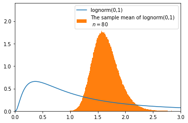
The validity of the Student’s $t$ method depends upon the Gaussianity of the sample mean, which, strictly speaking does not hold for any finite sample size unless the original distribution itself is Gaussian. However, for many applications, the sample mean becomes close enough to Gaussian as the sample size grows (due to the effects described by the central limit theorem), that the resulting bounds hold with probabilities close to the confidence level. Such results vary depending upon the unknown distribution, but it is generally accepted that a large enough sample size can be defined to cover any distributions that might occur in a given situation. The question is what to do when the sample size is smaller than such a threshold.

Establishing good confidence intervals on the mean for small samples is an important but often overlooked problem. The $t$-test is widely used in medical and social sciences. Small clinical trials (such as Phase 1 trials), where such tests could potentially be applied, occur frequently in practice (Institute of Medicine, 2001). In addition, there are several machine learning applications. The sample mean distribution of an importance-weighted estimator is skewed even when the sample size is much larger than $30$, so tighter bounds with guarantees may be beneficial. Algorithms in Safe Reinforcement Learning (Thomas et al., 2015) use importance weights to estimate the return of a policy and use confidence bounds to estimate the range of the mean. The UCB multi-armed bandit algorithm is designed using the Hoeffding bound - a tighter bound may lead to better performance with guarantees.

In the two-ended support setting, our bounds provide a new and better option for guaranteed coverage with small sample sizes. At least one version of our bound is tighter (or as tight) for every possible sample than the bound by Anderson (Anderson, 1969a), which is arguably the best existing bound with guaranteed coverage for small sample sizes. In the limit as $a\rightarrow-\infty$, i.e., the one-ended support setting, this version of our bound is equivalent to Anderson.

It can be shown from Learned-Miller & Thomas (2019) that Anderson’s UCB is less than or equal to Hoeffding’s for any sample when $\alpha\leq 0.5$, and is strictly less than Hoeffding’s when $\alpha\leq 0.5$ and $n\geq 3$. Therefore our bound is also less than or equal to Hoeffding’s for any sample when $\alpha\leq 0.5$, and is strictly better than Hoeffding’s inequality when $\alpha\leq 0.5$ and $n\geq 3$.

Below we review bounds with coverage guarantees, those that do not exhibit guaranteed coverage, and those for which the result is unknown.

1.1 Distribution free bounds with guaranteed coverage

Several bounds exist that have guaranteed coverage. These include Hoeffding’s inequality (Hoeffding, 1963), Anderson’s bound (Anderson, 1969a), and the bound due to Maurer & Pontil (2009).

Hoeffding’s inequality. For a distribution $F$ on $[a,b]$, Hoeffding’s inequality (Hoeffding, 1963) provides a bound on the probability that the sample mean, $\bar{X}_{n}=\frac{1}{n}\sum_{i=1}^{n}X_{i}$, will deviate from the mean by more than some amount $t\geq 0$:

$$\Pr\left(\mu-\bar{X}_{n}\leq t\right)\leq e^{-\frac{2nt^{2}}{(b-a)^{2}}}.$$ (2)

Defining $\alpha$ to be the right hand side of this inequality, solving for $t$ as a function of $\alpha$, and rewriting in terms of $\alpha$ rather than $t$, one obtains a $1-\alpha$ UCB on the mean of

$$b^{\alpha,\text{Hoeffding}}(\mathbf{X})\overset{\underset{\mathrm{def}}{}}{=}\bar{X}_{n}+(b-a)\sqrt{\frac{\ln(1/\alpha)}{2n}}.$$ (3)

Maurer and Pontil. One limitation of Hoeffding’s inequality is that the amount added to the sample mean to obtain the UCB scales with the range of the random variable over $\sqrt{n}$, which shrinks slowly as $n$ increases.

Bennett’s inequality (Bennett, 1962) considers both the sample mean and the sample variance and obtains a better dependence on the range of the random variable when the variance is known. Maurer & Pontil (2009) derived a UCB for the variance of a random variable, and suggest combining this with Bennet’s inequality (via the union bound) to obtain the following $1-\alpha$ UCB on the mean:

$$b^{\alpha,\text{M\&P}}(\mathbf{X})\overset{\underset{\mathrm{def}}{}}{=}\bar{X}_{n}+\frac{7(b-a)\ln(2/\alpha)}{3(n-1)}+\sqrt{\frac{2\hat{\sigma}^{2}\ln(2/\alpha)}{n}}.$$

Notice that Maurer and Pontil’s UCB scales with the range $(b-a)$, divided by $n$ (as opposed to the $\sqrt{n}$ of Hoeffding’s). However, the $\sqrt{n}$ dependence is unavoidable to some extent: Maurer and Pontil’s UCB scales with the sample standard deviation $\hat{\sigma}$ divided by $\sqrt{n}$. As a result, Maurer and Pontil’s bound tends to be tighter than Hoeffding’s when both $n$ is large and the range of the random variable is large relative to the variance. Lastly, notice that Maurer and Pontil’s bound requires $n{\geq}2$ for the sample standard deviation to be defined.

Anderson’s bound. Anderson (1969a) introduces a bound by defining an ‘envelope’ of equal width that, with high probability, contains the true CDF. The upper and lower extremes of such an envelope define the CDFs with the minimum and maximum attainable means for distributions that fit within the envelope, and thus bound the mean with high probability.

In practice, Anderson’s bound tends to be significantly tighter than Maurer and Pontil’s inequality unless the variance of the random variable is miniscule in comparison to the range of the random variable (and $n$ is sufficiently large). However, neither Anderson’s inequality nor Maurer and Pontil’s inequality strictly dominates the other. That is, neither upper bound is strictly less than or equal to the other in all cases. However, Anderson’s bound does dominate Hoeffding’s inequality (Learned-Miller & Thomas, 2019).

Some authors have proposed specific envelopes for use with Anderson’s technique (Diouf & Dufour, 2005; Learned-Miller & DeStefano, 2008; Romano & Wolf, 2000). However, none of these variations are shown to dominate Anderson’s original bound. That is, while they give tighter intervals for some samples, they are looser for others.

Other bounds. Fienberg et al. (1977) proposed a bound for distributions on a discrete set of support points, but nothing prevents it, in theory, from being applied to an arbitrarily dense set of points on an interval such as $[0,1]$. This bound has a number of appealing properties, and comes with a proof of guaranteed coverage. However, the main drawback is that it is currently computationally intractable, with a computation time that depends exponentially on the number of points in the support set, precluding many (if not most) practical applications.

In an independent concurrent work, Waudby-Smith & Ramdas (2021) proposed another confidence interval for the mean, which generalizes and improves upon Hoeffding’s inequality.

1.2 Bounds that do not exhibit guaranteed coverage

Many bounds that are used in practice are known to violate Eq. (1) for certain distributions. These include the aforementioned Student’s $t$ method, and various bootstrap procedures, such as the bias-corrected and accelerated (BCa) bootstrap and the percentile bootstrap. See Efron & Tibshirani (1993) for details of these methods. A simple explanation of the failure of bootstrap methods for certain distributions is given by Romano & Wolf (2000, pages 757–758). Presumably if one wants guarantees of Eq. (1), one cannot use these methods (unless one has extra information about the unknown distribution).

1.3 Bounds conjectured to have guaranteed coverage

There are at least two known bounds that perform well in practice but for which no proofs of coverage are known. One of these, used in accounting procedures, is the so-called Stringer bound (Stringer, 1963). It is known to violate Eq. (1) for confidence levels $\alpha>0.5$ (Pap & van Zuijlen, 1995), but its coverage for $\alpha<0.5$ is unknown.

A little known bound by Gaffke (2005) gives remarkably tight bounds on the mean, but has eluded a proof of guaranteed coverage. This bound was recently rediscovered by Learned-Miller & Thomas (2019), who do an empirical study of its performance and provide a method for computing it efficiently.

We demonstrate in Section 4 that our bound dominates those of both Hoeffding and Anderson. To our knowledge, this is the first bound that has been shown to dominate Anderson’s bound.

2 A Family of Confidence Bounds

In this section we define our new upper confidence bound. Let $n$ be the sample size. We use bold-faced letters to denote a vector of size $n$ and normal letters to denote a scalar. Uppercase letters denote random variables and lowercase letters denote values taken by them. For example, $X_{i}\in\mathcal{R}$ and $\mathbf{X}=(X_{1},...,X_{n})\in\mathcal{R}^{n}$ are random variables. $x_{i}\in\mathcal{R}$ is a value of $X_{i}$, and $\mathbf{x}=(x_{1},...,x_{n})\in\mathcal{R}^{n}$ is a value of $\mathbf{X}$. For a sample $\mathbf{x}$, we let $F(\mathbf{x})\overset{\underset{\mathrm{def}}{}}{=}(F(x_{1}),\cdots,F(x_{n}))\in[0,1]^{n}$.

Order statistics play a central role in our work. We denote random variable order statistics $X_{(1)}\leq X_{(2)}\leq...\leq X_{(n)}$ and of a specific sample as $x_{(1)}\leq x_{(2)}\leq...\leq x_{(n)}.$

Given a sample $\mathbf{X}=\mathbf{x}$ of size $n$ and a confidence level $1-\alpha$, we would like to calculate a UCB for the mean. Let $F$ be the CDF of $X_{i}$, i.e., the true distribution and $D\subset\mathcal{R}$ be the support of $F$. We assume that $D$ has a finite upper bound. Given $D$ and any function $T:D^{n}\rightarrow\mathcal{R}$ we will calculate an upper confidence bound $b^{\alpha}_{D,T}(\mathbf{x})$ for the mean of $F$.

We show in Lemma 2.1 that if ${D^{+}}$ is a superset of $D$ with finite upper bound, then $b^{\alpha}_{{D^{+}},T}(\mathbf{x})\geq b^{\alpha}_{D,T}(\mathbf{x})$. Therefore we only need to know a superset of the support with finite upper bound to obtain a guaranteed bound.

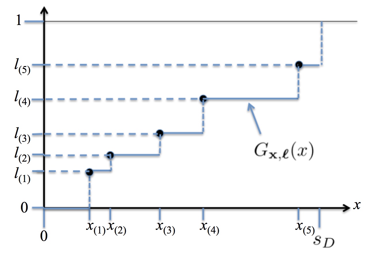
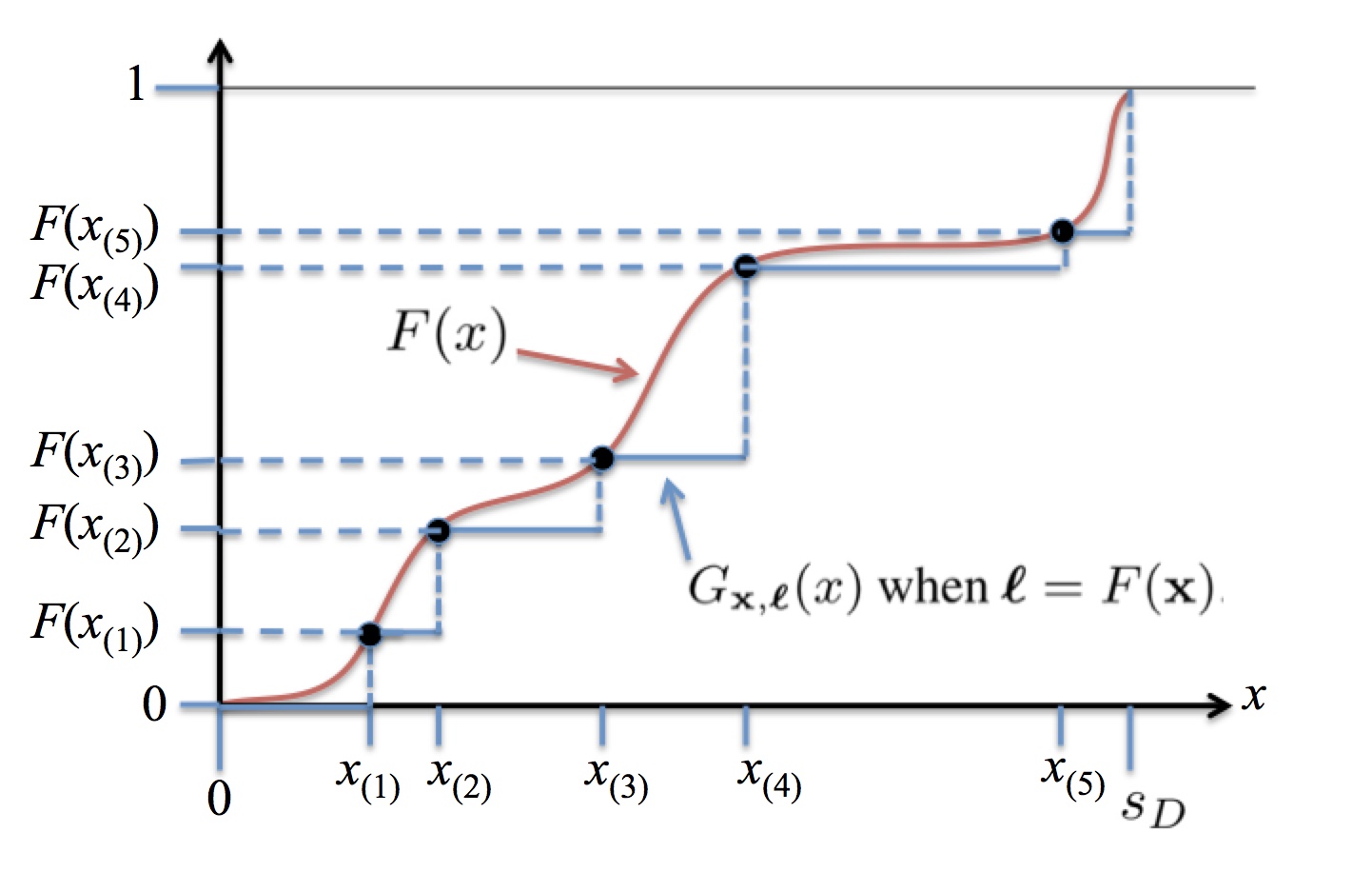
Let $s_{D}\overset{\underset{\mathrm{def}}{}}{=}\sup\{x:x\in D\}$. We next describe a method for pairing the sample $\mathbf{x}$ with another vector $\boldsymbol{\ell}\in[0,1]^{n}$ to produce a stairstep CDF function $G_{\mathbf{x},\boldsymbol{\ell}}$. Let $x_{(n+1)}\overset{\underset{\mathrm{def}}{}}{=}s_{D}$. Consider the step function $G_{\mathbf{x},\boldsymbol{\ell}}:\mathcal{R}\rightarrow[0,1]$ defined from $\boldsymbol{\ell}$ and $\mathbf{x}$ as follows (see Figure 1(a)):

$$G_{\mathbf{x},\boldsymbol{\ell}}(x)=\begin{cases}0,&\text{if }x<x_{(1)}\\ \ell_{(i)},&\text{if }x_{(i)}\leq x<x_{(i+1)}\\ 1,&\text{if }x\geq s_{D}.\end{cases}$$ (4)

In particular, when $\boldsymbol{\ell}=(1/n,\dotsc,n/n)$, $G_{\mathbf{x},\boldsymbol{\ell}}$ becomes the empirical CDF. Also note that when $\boldsymbol{\ell}=F(\mathbf{x})$, $\forall x,G_{\mathbf{x},\boldsymbol{\ell}}(x)\leq F(x)$, as illustrated in Figure 1(b).

(a) The stairstep function $G_{\mathbf{x},\boldsymbol{\ell}}$, which is a function of the sample $\mathbf{x}$ and a vector $\boldsymbol{\ell}$ of values between 0 and 1. When $\boldsymbol{\ell}=(1/n,\dotsc,n/n)$, $G_{\mathbf{x},\boldsymbol{\ell}}$ becomes the empirical CDF.

(b) The CDF of a distribution $F$ in red, with a random sample of five order statistics on the x-axis. The blue stairstep function shows the function $G_{\mathbf{x},\boldsymbol{\ell}}(x)$ when $\boldsymbol{\ell}=F(\mathbf{x})$. Notice that for all $x$, $G_{\mathbf{x},\boldsymbol{\ell}}(x)\leq F(x)$.

Figure 1:

Following Learned-Miller & Thomas (2019), if we consider $G_{\mathbf{x},\boldsymbol{\ell}}$ to be a CDF, we can compute the mean of the resulting distribution as a function of two vectors $\mathbf{x}$ and $\boldsymbol{\ell}$ as

$$m_{D}(\mathbf{x},\boldsymbol{\ell}) \overset{\underset{\mathrm{def}}{}}{=}\sum_{i=1}^{n+1}x_{(i)}(\ell_{(i)}-\ell_{(i-1)})$$ (5)

$$=s_{D}-\sum_{i=1}^{n}\ell_{(i)}(x_{(i+1)}-x_{(i)}),$$ (6)

where $\ell_{(0)}\overset{\underset{\mathrm{def}}{}}{=}0$, $\ell_{(n+1)}\overset{\underset{\mathrm{def}}{}}{=}1$ and $x_{(n+1)}\overset{\underset{\mathrm{def}}{}}{=}s_{D}$. When $s_{D}$ is finite, this is well-defined. Notice that this function is defined in terms of the order statistics of $\mathbf{x}$ and $\boldsymbol{\ell}$. Learned-Miller & Thomas (2019) refer to this as the induced mean for the sample $\mathbf{x}$ by the vector $\boldsymbol{\ell}$. Although we borrow the above terms from Learned-Miller & Thomas (2019), the bound we introduce below is a new class of bounds, and differs from the bounds discussed in their work.

An ordering on $D^{n}$. Next, we introduce a scalar-valued function $T$ which we will use to define a total order on samples in $D^{n}$, and define a set of samples less than or equal to another sample. In particular, for any function $T:\mathcal{R}^{n}\rightarrow\mathcal{R}$, let $\mathbb{S}_{D,T}(\mathbf{x})=\{\mathbf{y}\in D^{n}|T(\mathbf{y})\leq T(\mathbf{x})\}$.

The greatest induced mean for a given $\mathbf{U}$. Let $\mathbf{U}=U_{1},...,U_{n}$ be a sample of size $n$ from the continuous uniform distribution on $[0,1]$, with $\mathbf{u}\overset{\underset{\mathrm{def}}{}}{=}(u_{1},\cdots,u_{n})$ being a particular sample of $\mathbf{U}$.

Now consider the random quantity

$$b_{D,T}(\mathbf{x},\mathbf{U})\overset{\underset{\mathrm{def}}{}}{=}\sup_{\mathbf{z}\in\mathbb{S}_{D,T}(\mathbf{x})}m_{D}(\mathbf{z},\mathbf{U}),$$ (7)

which depends upon a fixed sample $\mathbf{x}$ (non-random) and also on the random variable $\mathbf{U}$.

Our upper confidence bound. Let $0<p<1$. Let $Q(p,Y)$ be the quantile function of the scalar random variable $Y$, i.e.,

$$Q(p,Y)\overset{\underset{\mathrm{def}}{}}{=}\inf\{y\in\mathbb{R}:F_{Y}(y)\geq p\},$$ (8)

where $F_{Y}(y)$ is the CDF of $Y$. We define $b^{\alpha}_{D,T}(\mathbf{x})$ to be the $(1-\alpha)$-quantile of the random quantity $b_{D,T}(\mathbf{x},\mathbf{U})$.

Definition 2.1 (Upper confidence bound on the mean).

Given a sample $\mathbf{x}$ and a confidence level $1-\alpha$:

$$b^{\alpha}_{D,T}(\mathbf{x})\overset{\underset{\mathrm{def}}{}}{=}Q(1-\alpha,b_{D,T}(\mathbf{x},\mathbf{U})),$$ (9)

where $b_{D,T}(\mathbf{x},\mathbf{U})$ is defined in Eq. 7.

To simplify notation, we drop the superscript and subscripts whenever clear. We show in Section 2.1 that this UCB has guaranteed coverage for all sample sizes $n$, for all confidence levels $0<1-\alpha<1$ and for all distributions $F$ and support $D$ where $s_{D}$ is finite.

We show below that a bound computed from a superset ${D^{+}}\supseteq D$ will be looser than or equal to a bound computed from the support $D$. Therefore it is enough to know a superset of the support $D$ to obtain a bound with guaranteed coverage.

Lemma 2.1.

Let ${D^{+}}\supseteq D$ where $s_{D^{+}}$ is finite. For any sample $\mathbf{x}$:

$$b^{\alpha}_{D}(\mathbf{x})\leq b^{\alpha}_{{D^{+}}}(\mathbf{x}).$$ (10)

Proof.

Since $s_{D^{+}}$ is finite, $m_{{D^{+}}}(\mathbf{y},\mathbf{\mathbf{u}})$ is well-defined. Since $D\subseteq{D^{+}}$, for any $\mathbf{y}$ and $\mathbf{u}$, $m_{D}(\mathbf{y},\mathbf{u})\leq m_{{D^{+}}}(\mathbf{y},\mathbf{u})$. Then

$$\sup_{\mathbf{y}\in\mathbb{S}_{D}(\mathbf{x})}m_{D}(\mathbf{y},\mathbf{\mathbf{u}}) \leq\sup_{\mathbf{y}\in\mathbb{S}_{D}(\mathbf{x})}m_{{D^{+}}}(\mathbf{y},\mathbf{\mathbf{u}})$$ (11)

$$\leq\sup_{\mathbf{y}\in\mathbb{S}_{{D^{+}}}(\mathbf{x})}m_{{D^{+}}}(\mathbf{y},\mathbf{\mathbf{u}}),$$ (12)

where the last inequality is because $\mathbb{S}_{D}(\mathbf{x})\subseteq\mathbb{S}_{{D^{+}}}(\mathbf{x})$. Let $b_{D}(\mathbf{x},\mathbf{U})=\sup_{\mathbf{z}\in\mathbb{S}_{D}(\mathbf{x})}m_{D}(\mathbf{z},\mathbf{U})$ and $b_{{D^{+}}}(\mathbf{x},\mathbf{U})=\sup_{\mathbf{z}\in\mathbb{S}_{{D^{+}}}(\mathbf{x})}m_{{D^{+}}}(\mathbf{z},\mathbf{U})$. Then $b^{\alpha}_{D}(\mathbf{x})$ and $b^{\alpha}_{{D^{+}}}(\mathbf{x})$ are the $(1-\alpha)$-quantiles of $b_{D}(\mathbf{x},\mathbf{U})$ and $b_{{D^{+}}}(\mathbf{x},\mathbf{U})$. Since $b_{D}(\mathbf{x},\mathbf{u})\leq b_{{D^{+}}}(\mathbf{x},\mathbf{u})$ for any $\mathbf{u}$, $b_{D}^{\alpha}(\mathbf{x})\leq b^{\alpha}_{{D^{+}}}(\mathbf{x})$. ∎

In Section 2.1 we show that the bound has guaranteed coverage. In Section 3 we discuss how to efficiently compute the bound. In Section 4 we show that when $T$ is a certain linear function, the bound is equal to or tighter than Anderson’s for any sample. In addition, we show that when the support is known to be $\{0,1\}$, our bound recovers the well-known Clopper-Pearson confidence bound for binomial distributions (Clopper & Pearson, 1934). In Section 5, we present simulations that show the consistent superiority of our bounds over previous bounds.

2.1 Guaranteed Coverage

In this section we show that our bound has guaranteed coverage in Theorem 2.7. We omit superscripts and subscripts if they are clear from context.

2.1.1 Preview of proof

Figure 2: Illustrations of Section 2.1.1. Left. The yellow region shows samples of $\mathbf{z}=[z_{(1)},z_{(2)}]$ such that $b^{\alpha}(\mathbf{z})\leq b^{\alpha}(\mathbf{x}_{max})$. Right. The same yellow region, but in the coordinates $\mathbf{u}=F^{-1}(\mathbf{z})$. We will show that the yellow region is a subset of the striped, which contains $\mathbf{u}$ such that $b(\mathbf{x}_{max},\mathbf{u})\geq\mu$.

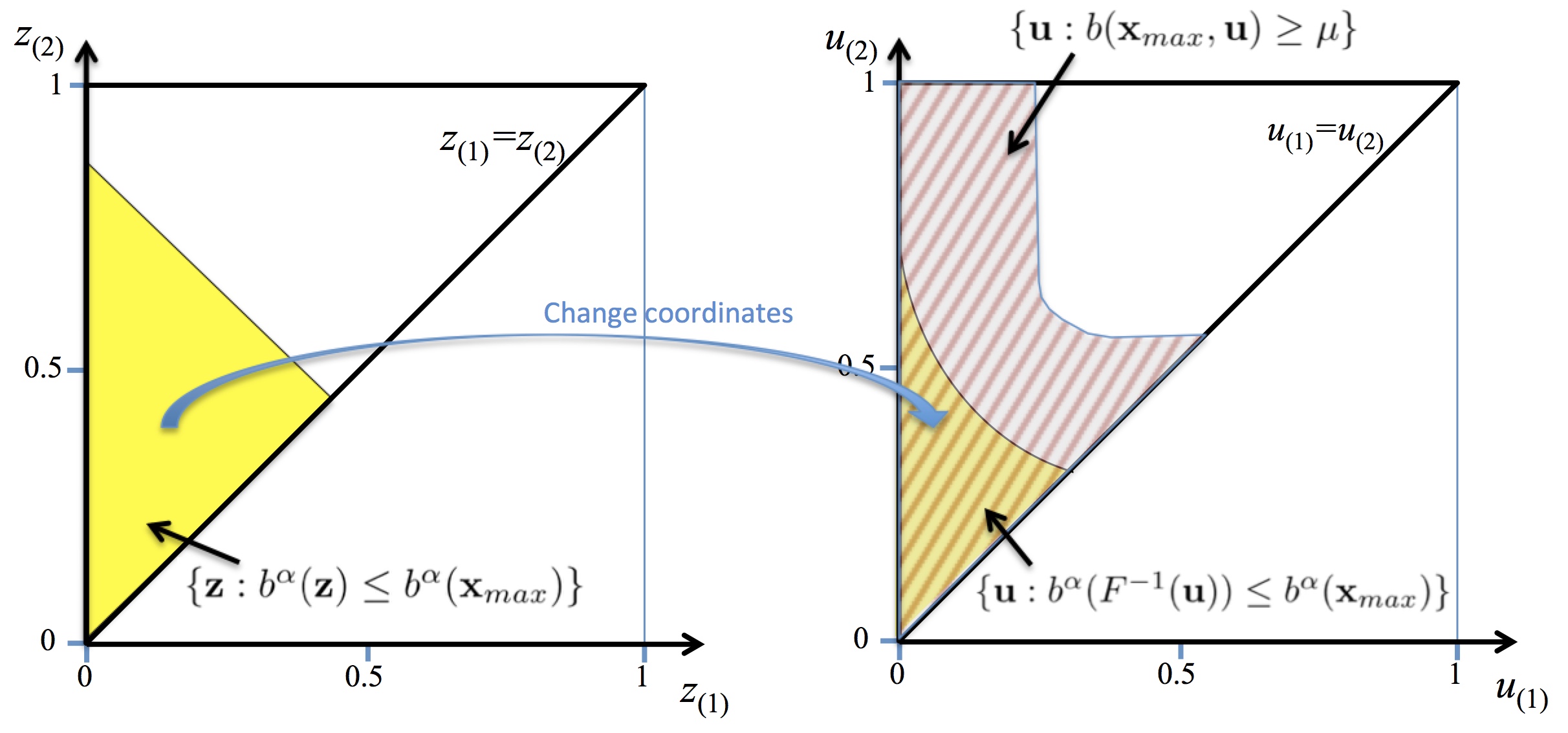
We explain the idea behind our bound at a high level using a special case. Note that our proof is more general than our special case, which makes assumptions such as the continuity of $F$ to simplify the intuition.

Suppose that $F$ is continuous. Then the probability integral transform $F_{X}(X)$ of $X$ is uniformly distributed on $[0,1]$ (Angus, 1994). Suppose there exists a sample $\mathbf{x}_{\mu}$ such that $b^{\alpha}(\mathbf{x}_{\mu})=\mu$. Then the probability that a sample $\mathbf{Z}$ outputs $b^{\alpha}(\mathbf{Z})<\mu$ is equal to the probability $\mathbf{Z}$ outputs $b^{\alpha}(\mathbf{Z})<b^{\alpha}(\mathbf{x}_{\mu})$ (the yellow region on the left of Fig. 2). This is the region where the bound fails, and we would like to show that the probability of this region is at most $\alpha$.

Let $\mathbf{U}\overset{\underset{\mathrm{def}}{}}{=}F(\mathbf{Z})$ and $\mathbf{u}\overset{\underset{\mathrm{def}}{}}{=}F(\mathbf{z})$. Then $U_{i}$ is uniformly distributed on $[0,1]$. If $F$ is invertible, we can transform the region $\{\mathbf{z}:b^{\alpha}(\mathbf{z})<b^{\alpha}(\mathbf{x}_{\mu})\}$ to $\{\mathbf{u}:b^{\alpha}(F^{-1}(\mathbf{u}))<b^{\alpha}(\mathbf{x}_{\mu})\}$ where $F^{-1}(\mathbf{u})\overset{\underset{\mathrm{def}}{}}{=}(F^{-1}(u_{1}),\dotsc,F^{-1}(u_{n}))$ (the yellow region on the right of Fig. 2).

Through some calculations using the definition of function $b$, we can show that the yellow region $\{\mathbf{u}:b^{\alpha}(F^{-1}(\mathbf{u}))<b^{\alpha}(\mathbf{x}_{\mu})\}$ is a subset of the striped region $\{\mathbf{u}:b(\mathbf{x}_{\mu},\mathbf{u})\geq\mu\}$.

Note that since $b^{\alpha}(\mathbf{x}_{\mu})=\mu$, $\mu$ is equal to the $1-\alpha$ quantile of $b(\mathbf{x}_{\mu},\mathbf{U})$. Therefore, by the definition of quantile, the probability of the striped region is at most $\alpha$:

$$\mathbb{P}_{\mathbf{U}}(b(\mathbf{x}_{\mu},\mathbf{U})\geq\mu)\leq\alpha,$$ (13)

and thus the probability of the yellow region is at most $\alpha$.

2.1.2 Main Result

In this section, we present some supporting lemmas and then the main result in Theorem 2.7. The proofs of the simpler lemmas have been deferred to the supplementary material.

Lemma 2.2.

Let $X$ be a random variable with CDF $F$ and $Y\overset{\underset{\mathrm{def}}{}}{=}F(X)$, known as the probability integral transform of $X$. Let $U$ be a uniform random variable on $[0,1]$. Then for any $0\leq y\leq 1$,

$$\mathbb{P}(Y\leq y)\leq\mathbb{P}(U\leq y).$$ (14)

If $F$ is continuous, then $Y$ is uniformly distributed on $[0,1]$.

In the next lemma we show that the mean satisfies the following property. Let $F$ and $G$ be two CDF functions such that $F(x)$ is always larger than or equal to $G(x)$ for all $x$. Then the mean of $F$ is smaller than the mean of $G$.

Lemma 2.3.

Let $F$ and $G_{\mathbf{x},\boldsymbol{\ell}}$ be two CDF functions such that $\forall x\in\mathcal{R}$, $F(x)\geq G_{\mathbf{x},\boldsymbol{\ell}}(x)$. Let $\mu_{F}$ and $\mu_{G}$ denote the means of $F$ and $G_{\mathbf{x},\boldsymbol{\ell}}$. Then

$$\mu_{F}\leq\mu_{G}.$$ (15)

For use in the next lemma, we define a partial order for the samples on $D^{n}$. Note that it is defined with respect to the order statistics of the sample, not the original components.

Definition 2.2 (Partial Order).

For any two samples $\mathbf{z}$ and $\mathbf{y}$, we define $\mathbf{z}\preceq\mathbf{y}$ to indicate that ${z}_{(i)}\leq{y}_{(i)},1\leq i\leq n$.

Lemma 2.4.

Let $\mathbf{Z}$ be a random sample of size $n$ from $F$. Let $\mathbf{U}=U_{1},...,U_{n}$ be a sample of size $n$ from the continuous uniform distribution on $[0,1]$. For any function $T:D^{n}\rightarrow R$ and any $\mathbf{x}\in D^{n}$:

$$\mathbb{P}_{\mathbf{Z}}(T(\mathbf{Z})\leq T(\mathbf{x}))\leq\mathbb{P}_{\mathbf{U}}(b(\mathbf{x},\mathbf{U})\geq\mu).$$ (16)

Proof sketch.

Let $\cup$ denote the union of events and $\{\}$ denote an event. Then for any $\mathbf{x}\in D^{n}$:

$$\mathbb{P}_{\mathbf{Z}}(T(\mathbf{Z})\leq T(\mathbf{x})) = \mathbb{P}_{\mathbf{Z}}(\mathbf{Z}\in\mathbb{S}(\mathbf{x}))$$ (17)

$$= \mathbb{P}_{\mathbf{Z}}(\cup_{\mathbf{y}\in\mathbb{S}(\mathbf{x})}\{\mathbf{Z}=\mathbf{y}\})$$ (18)

$$\leq \mathbb{P}_{\mathbf{Z}}(\cup_{\mathbf{y}\in\mathbb{S}(\mathbf{x})}\{\mathbf{Z}\preceq\mathbf{y}\})$$ (19)

$$\leq \mathbb{P}_{\mathbf{Z}}(\cup_{\mathbf{y}\in\mathbb{S}(\mathbf{x})}\{F(\mathbf{Z})\preceq F(\mathbf{y})\})\text{ by monotone $F$}\;\;\;$$ (20)

$$\leq \mathbb{P}_{\mathbf{U}}(\cup_{\mathbf{y}\in\mathbb{S}(\mathbf{x})}\{\mathbf{U}\preceq F(\mathbf{y})\}).$$ (21)

The last step is by an extension of Lemma 2.2. Recall that $m_{D}(\mathbf{y},\mathbf{u})=s_{D}-\sum_{i=1}^{n}u_{(i)}(y_{(i+1)}-y_{(i)})$ where $\forall i,y_{(i+1)}-y_{(i)}\geq 0$. Therefore if $\mathbf{u}\preceq F(\mathbf{y})$ then $m_{D}(\mathbf{y},\mathbf{u})\geq m_{D}(\mathbf{y},F(\mathbf{y}))$:

$$\mathbb{P}_{\mathbf{U}}(\cup_{\mathbf{y}\in\mathbb{S}(\mathbf{x})}\{\mathbf{U}\preceq F(\mathbf{y})\}) \leq \mathbb{P}_{\mathbf{U}}(\cup_{\mathbf{y}\in\mathbb{S}(\mathbf{x})}\{m_{D}(\mathbf{y},\mathbf{U})\geq m_{D}(\mathbf{y},F(\mathbf{y}))\}),\text{by Lemma~{}\ref{lem:helper2}}$$ (22)

$$\leq \mathbb{P}_{\mathbf{U}}(\cup_{\mathbf{y}\in\mathbb{S}(\mathbf{x})}\{m_{D}(\mathbf{y},\mathbf{U})\geq\mu\}),\text{by Lemma~{}\ref{lem:helper2}}\hskip 14.45377pt$$ (23)

$$\leq \mathbb{P}_{\mathbf{U}}(\sup_{\mathbf{y}\in\mathbb{S}(\mathbf{x})}m_{D}(\mathbf{y},\mathbf{U})\geq\mu)$$ (24)

$$= \mathbb{P}_{\mathbf{U}}(b(\mathbf{x},\mathbf{U})\geq\mu).$$ (25)

∎

We include a more detailed version of the proof for the above lemma in the supplementary material.

Lemma 2.5.

Let $\mathbf{U}=U_{1},...,U_{n}$ be a sample of size $n$ from the continuous uniform distribution on $[0,1]$. Let $\mathbf{X}$ and $\mathbf{Z}$ denote i.i.d. samples of size $n$ from $F$. For any function $T:D^{n}\rightarrow\mathcal{R}$ and any $\alpha\in(0,1)$,

$$\mathbb{P}_{\mathbf{X}}\left(\mathbb{P}_{\mathbf{U}}(b_{D,T}(\mathbf{X},\mathbf{U})\geq\mu)\leq\alpha\right) \leq\mathbb{P}_{\mathbf{X}}\left(\mathbb{P}_{\mathbf{Z}}(T(\mathbf{Z})\leq T(\mathbf{X}))\leq\alpha\right).$$

Proof.

From Lemma 2.4 for any sample $\mathbf{x}$,

$$\mathbb{P}_{\mathbf{Z}}(T(\mathbf{Z})\leq T(\mathbf{x}))\leq\mathbb{P}_{\mathbf{U}}(b(\mathbf{x},\mathbf{U})\geq\mu).$$ (26)

Therefore,

$$\mathbb{P}_{\mathbf{X}}\left(\mathbb{P}_{\mathbf{Z}}(T(\mathbf{Z})\leq T(\mathbf{X}))\leq\alpha\right) \geq\mathbb{P}_{\mathbf{X}}\left(\mathbb{P}_{\mathbf{U}}(b(\mathbf{X},\mathbf{U})\geq\mu)\leq\alpha\right).$$ (27)

∎

Lemma 2.6.

Let $\mathbf{U}=U_{1},...,U_{n}$ be a sample of size $n$ from the continuous uniform distribution on $[0,1]$. Let $\mathbf{X}$ be a random sample of size $n$ from $F$. For any function $T:D^{n}\rightarrow\mathcal{R}$ and any $\alpha\in(0,1)$,

$$\mathbb{P}_{\mathbf{X}}(b_{D,T}^{\alpha}(\mathbf{X})<\mu) \leq\mathbb{P}_{\mathbf{X}}\left(\mathbb{P}_{\mathbf{U}}(b_{D,T}(\mathbf{X},\mathbf{U})\geq\mu)\leq\alpha\right).$$ (28)

Proof.

Because $b^{\alpha}(\mathbf{x})$ is the $1-\alpha$ quantile of $b(\mathbf{x},\mathbf{U})$, by the definition of quantile: $\mathbb{P}_{\mathbf{U}}(b(\mathbf{x},\mathbf{U})\leq b^{\alpha}(\mathbf{x}))\geq 1-\alpha$. Therefore $\mathbb{P}_{\mathbf{U}}(b(\mathbf{x},\mathbf{U})\geq b^{\alpha}(\mathbf{x}))\leq\alpha.$ If $b^{\alpha}(\mathbf{x})<\mu$ then $\mathbb{P}_{\mathbf{U}}(b(\mathbf{x},\mathbf{U})\geq\mu)\leq\alpha.$ Since $b^{\alpha}(\mathbf{x})<\mu$ implies $\mathbb{P}_{\mathbf{U}}(b(\mathbf{x},\mathbf{U})\geq\mu)\leq\alpha$, we have

$$\mathbb{P}_{\mathbf{X}}(b^{\alpha}(\mathbf{X})<\mu) \leq\mathbb{P}_{\mathbf{X}}\left(\mathbb{P}_{\mathbf{U}}(b(\mathbf{X},\mathbf{U})\geq\mu)\leq\alpha\right).$$ (29)

∎

We now show that the bound has guaranteed coverage.

Theorem 2.7.

Let $\mathbf{X}$ be a random sample of size $n$ from $F$. For any function $T:D^{n}\rightarrow R$ and for any $\alpha\in(0,1)$:

$$\mathbb{P}_{\mathbf{X}}(b^{\alpha}_{D,T}(\mathbf{X})<\mu)\leq\alpha.$$ (30)

Proof.

Let $\mathbf{Z}$ be a random sample of size $n$ from $F$.

$$\mathbb{P}_{\mathbf{X}}(b^{\alpha}(\mathbf{X})<\mu) \leq\mathbb{P}_{\mathbf{X}}\left(\mathbb{P}_{\mathbf{U}}(b(\mathbf{X},\mathbf{U})\geq\mu)\leq\alpha\right)\text{ by Lemma~{}\ref{lem:helper3}}$$ (31)

$$\leq\mathbb{P}_{\mathbf{X}}\left(\mathbb{P}_{\mathbf{Z}}(T(\mathbf{Z})\leq T(\mathbf{X}))\leq\alpha\right)\text{ by Lemma~{}\ref{lem:helper4}}$$ (32)

$$=\mathbb{P}\left(W\leq\alpha\right)\text{ where }W\overset{\underset{\mathrm{def}}{}}{=}\mathbb{P}_{\mathbf{Z}}(T(\mathbf{Z})\leq T(\mathbf{X}))$$ (33)

$$\leq\alpha\text{ by Lemma~{}\ref{lem:CDF_vs_U}}.$$ (34)

∎

3 Computation

In this section we present a Monte Carlo algorithm to compute the bound. First we note that since the bound only depends on $\mathbf{x}$ via the function $T(\mathbf{x})$, we can precompute a table of the bounds for each value of $T(\mathbf{x})$. We discuss how to adjust for the uncertainty in the Monte Carlo result in Appendix D.

Algorithm 1 Monte Carlo estimation of $m^{\alpha}_{D^{+},T}(\mathbf{x})$ where $D^{+}=[0,1]$. This pseudocode uses 1-based array indexing.

  Input: A sample $\mathbf{x}\in D^{n}$, confidence parameter $1-\alpha<1$, a function $T:[0,1]^{n}\rightarrow\mathcal{R}$ and Monte Carlo sampling parameter $l$.

  Output: An estimation of $m^{\alpha}_{D^{+},T}(\mathbf{x})$ $n\leftarrow length(\mathbf{x})$.

  Create array ms to hold $l$ floating point numbers, and initialize it to zero.

  Create array u to hold $n$ floating point numbers.

  for $i\leftarrow 1$ to $l$ do

     for $j\leftarrow 1$ to $n$ do

        u[j] $\sim$ Uniform(0,1).

     end for

     Sort(u, ascending).

     Solve: $M=\max_{y_{(1)},\cdots,y_{(n)}}m(\mathbf{y},\mathbf{u})$ subject to:

        1) $T(\mathbf{y})\leq T(\mathbf{x})$.

        2) $~{}\forall i:1\leq i\leq n,0\leq y_{(i)}\leq 1$.

        3) $y_{(1)}\leq y_{(2)}\leq...\leq y_{(n)}$.

     $\mathbf{ms}[i]=M$.

  end for

  Sort(ms, ascending).

  Return $\mathbf{ms}[\lceil(1-\alpha)l\rceil]$.

Let the superset of the support $D^{+}$ be a closed interval with a finite upper bound. If $m$ is a continuous function,

$$\sup_{\mathbf{y}\in\mathbf{S}_{D^{+}}(\mathbf{x})}m(\mathbf{y},\mathbf{u})=\max_{\mathbf{y}\in\mathbf{S}_{D^{+}}(\mathbf{x})}m(\mathbf{y},\mathbf{u}).$$ (35)

Therefore $b_{D^{+}}(\mathbf{x},\mathbf{u})$ is the solution to

$$\max_{y_{(1)},\dotsc,y_{(n)}}m(\mathbf{y},\mathbf{u})$$ (36)

subject to:

1. $T(\mathbf{y})\leq T(\mathbf{x})$,

2. $~{}\forall i\in\{1,\dotsc,n\},y_{(i)}\in{D^{+}}$,

3. $y_{(1)}\leq y_{(2)}\leq\cdots\leq y_{(n)}$.

When $D^{+}$ is an interval and $T$ is linear, this is a linear programming problem and can be solved efficiently.

We can compute the $1-\alpha$ quantile of a random variable $M$ using Monte Carlo simulation, sampling $M$ $l$ times. Letting $m_{(1)}\leq...\leq m_{(l)}$ be the sorted values, we output $m_{(\lceil(1-\alpha)l\rceil)}$ as an approximation of the $1-\alpha$ quantile.

Running time. Note that since the bound only depends on $\mathbf{x}$ via the function $T(\mathbf{x})$, we can precompute a table of the bounds for each value of $T(\mathbf{x})$ to save time. When $T$ is linear, the algorithm needs to solve a linear programming problem with $n$ variables and $2n$ constraints $l$ times. For sample size $n=50$, computing the bound for each sample $\mathbf{x}\in D^{n}$ takes just a few seconds using $l=10,\!000$ Monte Carlo samples.

4 Relationships with Existing Bounds

In this section, we compare our bound to previous bounds including those of Clopper and Pearson, Hoeffding, and Anderson. Proofs omitted in this section can be found in the supplementary material.

4.1 Special Case: Bernoulli Distribution

When we know that $D=\{0,1\}$, the distribution is Bernoulli. If we choose $T$ to be the sample mean, our bound becomes the same as the Clopper-Pearson confidence bound for binomial distributions (Clopper & Pearson, 1934). See the supplementary material for details.

4.2 Comparisons with Anderson and Hoeffding

In this section we show that for any sample size $n$, any confidence level $\alpha$ and for any sample $\mathbf{x}$, our method produces a bound no larger than Anderson’s bound (Theorem 4.3) and Hoeffding’s bound (Theorem 4.4).

Note that if we only know an upper bound $b$ of the support (1-ended support setting), we can set ${D^{+}}=(-\infty,b]$ and our method is equal to Anderson’s (Appendix E.3) and dominates Hoeffding’s. As the lower support bound increases (2-ended setting), our bound becomes tighter or remains constant, whereas Anderson’s remains constant, as it does not incorporate information about a lower support. Thus, in cases where our bound can benefit from a lower support, we are tighter than Anderson’s.

Anderson’s bound constructs an upper bound for the mean by constructing a lower bound for the CDF. We defined a lower bound for the CDF as follows.

Definition 4.1 (Lower confidence bound for the CDF).

Let $\mathbf{X}=(X_{1},\cdots,X_{n})$ be a sample of size $n$ from the distribution on $\mathcal{D}^{+}$ with unknown CDF $F$. Let $\alpha\in(0,1)$. Let $H_{\mathbf{X}}:\mathcal{R}\rightarrow[0,1]$ be a function computed from the sample $\mathbf{X}$ such that for any CDF $F$,

$$\mathbb{P}_{\mathbf{X}}(~{}\forall x\in R,F(x)\geq H_{\mathbf{X}}(x))\geq 1-\alpha.$$ (37)

Then $H_{\mathbf{X}}$ is called a $(1-\alpha)$ lower confidence bound for the CDF.

If there exists a CDF $F$ such that

$$\mathbb{P}_{\mathbf{X}}(~{}\forall x\in R,F(x)\geq H_{\mathbf{X}}(x))=1-\alpha,$$ (38)

then $H_{\mathbf{X}}$ is called an exact $(1-\alpha)$ lower confidence bound for the CDF.

In Figs. 1(a) and 1(b), it is easy to see that if the stairstep function $G_{\mathbf{X},\boldsymbol{\ell}}$ is a lower confidence bound for the CDF then its induced mean $m(\mathbf{X},\boldsymbol{\ell})$ is an upper confidence bound for $\mu$.

Lemma 4.1.

Let $\mathbf{X}=(X_{1},\cdots,X_{n})$ be a sample of size $n$ from a distribution with mean $\mu$. Let $\boldsymbol{\ell}\in[0,1]^{n}$. If $G_{\mathbf{X},\boldsymbol{\ell}}$ is a $(1-\alpha)$ lower confidence bound for the CDF then

$$\mathbb{P}_{\mathbf{X}}(m(\mathbf{X},\boldsymbol{\ell})\geq\mu)\geq 1-\alpha.$$ (39)

Let $U_{(i)},1\leq i\leq n$ be the order statistics of the uniform distribution. Note that for any CDF $F$:

$$\mathbb{P}_{\mathbf{X}}(~{}\forall x\in\mathcal{R},F(x)\geq G_{\mathbf{X},\boldsymbol{\ell}}(x)) =\mathbb{P}_{\mathbf{X}}(\forall i:1\leq i\leq n,F(X_{(i)})\geq\ell_{(i)})$$ (40)

$$\geq\mathbb{P}_{\mathbf{U}}(\forall i:1\leq i\leq n,U_{(i)}\geq\ell_{(i)})\text{ by Lemma~{}\ref{lem:CDF_vs_U}},$$ (41)

where Eq. 41 is an equality if $F$ is the CDF of a continuous random variable. Therefore $G_{\mathbf{X},\boldsymbol{\ell}}$ is an exact $(1-\alpha)$ lower confidence bound for the CDF is equivalent to $\boldsymbol{\ell}$ satisfying:

$$\mathbb{P}_{\mathbf{U}}(\forall i:1\leq i\leq n,U_{(i)}\geq\ell_{(i)})=1-\alpha.$$ (42)

Anderson (1969a) presents $b^{\alpha,\text{Anderson}}_{\boldsymbol{\ell}}(\mathbf{x})=m_{D^{+}}(\mathbf{x},\boldsymbol{\ell})$ as a UCB for $\mu$ where $\boldsymbol{\ell}\in[0,1]^{n}$ is a vector such that $G_{\mathbf{X},\boldsymbol{\ell}}$ is an exact $(1-\alpha)$ lower confidence bound for the CDF.

In one instance of Anderson’s bound, $\boldsymbol{\ell}=\mathbf{u}^{And}\in[0,1]^{n}$ is defined as

$$u^{\text{And}}_{i}\overset{\underset{\mathrm{def}}{}}{=}\max\left\{0,i/n-\beta(n)\right\}.$$ (43)

Anderson identifies $\beta(n)$ as the one-sided Kolmogorov-Smirnov statistic such that $G_{\mathbf{X},\boldsymbol{\ell}}$ is an exact $(1-\alpha)$ lower confidence bound for the CDF when $\boldsymbol{\ell}=\mathbf{u}^{\text{And}}$. $\beta(n)$ can be computed by Monte Carlo simulation (Appendix A).

Learned-Miller & Thomas (2019) show that for any sample $\mathbf{x}$, a looser version of Anderson’s bound is better than Hoeffding’s:

Lemma 4.2 (from Theorem $2$ from (Learned-Miller & Thomas, 2019)).

For any sample size $n$, for any sample value $\mathbf{x}\in D^{n}$, for all $\alpha\in(0,0.5]$:

$$b^{\alpha,\text{Anderson}}_{\boldsymbol{\ell}}(\mathbf{x})\leq b^{\alpha,\text{Hoeffding}}(\mathbf{x}),$$ (44)

where $\boldsymbol{\ell}$ is defined as

$$\ell_{i}\overset{\underset{\mathrm{def}}{}}{=}\max\left\{0,i/n-\sqrt{\ln(1/\alpha)/(2n)}\right\}.$$ (45)

When $\alpha\leq 0.5$, this definition of $\boldsymbol{\ell}$ satisfies $G_{\mathbf{X},\boldsymbol{\ell}}$ is a $(1-\alpha)$ lower confidence bound for the CDF.

The inequality in Eq. 44 is strict for $n\geq 3$.

We show below that our bound is always equal to or tighter than Anderson’s bound. Appendix E.3 provides a more detailed analysis showing that our bound is equal to Anderson’s when the lower bound of the support is too small and can be tighter than Anderson’s when the lower bound of the support is large enough.

Theorem 4.3.

Let $\boldsymbol{\ell}\in[0,1]^{n}$ be a vector satisfying $G_{\mathbf{X},\boldsymbol{\ell}}$ is an exact $(1-\alpha)$ lower confidence bound for the CDF.

Let $D^{+}=(-\infty,b]$. For any sample size $n$, for any sample value $\mathbf{x}\in D^{n}$, for all $\alpha\in(0,1)$, using $T(\mathbf{x})=b^{\alpha,\text{Anderson}}_{\boldsymbol{\ell}}(\mathbf{x})$ yields

$$b^{\alpha}_{D^{+},T}(\mathbf{x})\leq b^{\alpha,\text{Anderson}}_{\boldsymbol{\ell}}(\mathbf{x}).$$ (46)

We explain briefly why this is true. First, from Figure 1(b), we can see that if $G_{\mathbf{X},\boldsymbol{\ell}}$ is a lower confidence bound then $\forall i,F(X_{(i)})\geq\ell_{(i)}$. Note that $G_{\mathbf{X},\boldsymbol{\ell}}$ must be a lower bound for all unknown CDFs $F$, so we can pick a continuous $F$ where, according to Lemma 2.2, $U\overset{\underset{\mathrm{def}}{}}{=}F(X)$ is uniformly distributed on $[0,1]$. Therefore $\boldsymbol{\ell}$ satisfies

$$\mathbb{P}_{\mathbf{U}}(\forall i,U_{(i)}\geq\ell_{(i)})\geq 1-\alpha,$$ (47)

where the $U_{(i)}$’s are the order statistics of the uniform distribution. Since $b(\mathbf{x},\mathbf{U})$ is defined from linear functions of $\mathbf{U}$ with negative coefficients (Eq. 6), if $\forall i,U_{(i)}\geq\ell_{(i)}$ then $b(\mathbf{x},\mathbf{U})\leq b(\mathbf{x},\boldsymbol{\ell})$. Therefore with probability at least $1-\alpha$, $b(\mathbf{x},\mathbf{U})\leq b(\mathbf{x},\boldsymbol{\ell})$. So $b(\mathbf{x},\boldsymbol{\ell})$ is at least the $1-\alpha$ quantile of $b(\mathbf{x},\mathbf{U})$, which is the value of our bound. Therefore $b(\mathbf{x},\boldsymbol{\ell})$ is at least the value of our bound.

Finally, if $T$ is Anderson’s bound, through some calculations we can show that $b_{D^{+},T}(\mathbf{x},\boldsymbol{\ell})=m_{D^{+}}(\mathbf{x},\boldsymbol{\ell})$, which is Anderson’s bound. The result follows.

Figure 3: The expected value of the bounds for $\alpha=0.05$ and $D^{+}=[0,1]$. For each sample size, we sample $\mathbf{X}$ $10,\!000$ times, compute the bound for each sample, and take the average. Our new bound with $T$ being Anderson’s bound consistently has lower expected value than Anderson’s (Theorem 4.3), Hoeffding’s (Theorem 4.4) and Maurer and Pontil’s. With $T$ being the $l2$-norm, the bound is substantially tighter in these examples, and also has guaranteed coverage.

Figure 4: The $\alpha$-quantile of the bound distribution for $\alpha=0.05$ and $D^{+}=[0,1]$. For each sample size, we sample $\mathbf{X}$ $10,\!000$ times, compute the bound for each sample, and take the $\alpha$ quantile. If the $\alpha$-quantile is below the true mean, the bound does not have guaranteed coverage. For the ${\tt uniform}(0,1)$ and ${\tt beta}(1,5)$ distribution, when the sample size is small, Student-t does not have guarantee.

The comparison with Hoeffding’s bound follows directly from Lemma 4.2 and Theorem 4.3:

Theorem 4.4.

Let $D^{+}=(-\infty,b]$. For any sample size $n$, for any sample value $\mathbf{x}\in D^{n}$, for all $\alpha\in(0,0.5]$, using $T(\mathbf{x})=b^{\alpha,\text{Anderson}}_{\boldsymbol{\ell}}(\mathbf{x})$ where $\boldsymbol{\ell}=\mathbf{u}^{\text{And}}$ yields:

$$b^{\alpha}_{D^{+},T}(\mathbf{x})\leq b^{\alpha,\text{Hoeffding}}(\mathbf{x}),$$ (48)

where the inequality is strict when $n\geq 3$.

Diouf & Dufour (2005) present several instances of Anderson’s bound with different $\boldsymbol{\ell}$ computed from the Anderson-Darling or the Eicker statistics (Theorem $4$, $5$ and Theorem $6$ with constant $\epsilon$).

Note that the result from Theorem 4.3 can be generalized for bounds $m(\mathbf{X},\boldsymbol{\ell})$ constructed from a $(1-\alpha)$ confidence lower bound $G_{\mathbf{X},\boldsymbol{\ell}}$ using Lemma 4.1. We show the general case in the supplementary material.

5 Simulations

We perform simulations to compare our bounds to Hoeffding’s inequality, Anderson’s bound, Maurer and Pontil’s, and Student-t’s bound (Student, 1908), the latter being

$$b^{\alpha,\text{Student}}(\mathbf{X})\overset{\underset{\mathrm{def}}{}}{=}\bar{X}_{n}+\sqrt{\frac{\hat{\sigma}^{2}}{n}}t_{1-\alpha,n-1}.$$ (49)

We compute Anderson’s bound with $\boldsymbol{\ell}=\mathbf{u}^{And}$ defined in Eq. 43 through Monte Carlo simulation (described in Appendix A). We use $\alpha=0.05$, $D^{+}=[0,1]$ and $l=10,\!000$ Monte Carlo samples. We consider two functions $T$:

1. Anderson: $T(\mathbf{x})=b^{\alpha,\text{Anderson}}_{\boldsymbol{\ell}}(\mathbf{x})$, again with $\boldsymbol{\ell}=\mathbf{u}^{And}$. Because this $T$ is linear in $\mathbf{x}$, it can be computed with the linear program in Eq. 35.

2. $l2$ norm: $T(\mathbf{x})=(\sum_{i=1}^{n}x^{2}_{i})/n$. In this case, $T$ requires the optimization of a linear functional over a convex region, which results in a simple convex optimization problem.

We perform experiments on three distributions: ${\tt beta}(1,5)$ (skewed right), ${\tt uniform}(0,1)$ and ${\tt beta}(5,1)$ (skewed left). Their PDFs are included in the supplementary material for reference. Additional experiments are in the supplementary material.

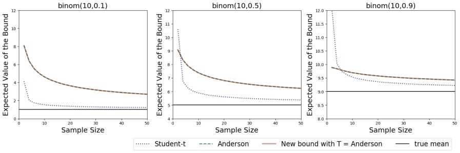
In Figure 3 and Figure 4 we plot the expected value and the $\alpha$-quantile value of the bounds as the sample size increases. Consistent with Theorem 4.3, our bound with $T$ being Anderson’s bound outperforms Anderson’s bound. Our new bound performs better than Anderson’s in distributions that are skewed right, and becomes similar to Anderson’s in left-skewed distributions. Our bound outperforms Hoeffding and Maurer and Pontil’s for all three distributions. Student-t fails (the error rate exceeds $\alpha$) for ${\tt beta}(1,5)$ and ${\tt uniform}(0,1)$ when the sample size is small (Figure 4).

Acknowledgements

This work was partially supported by DARPA grant FA8750-18-2-0117. Research reported in this paper was sponsored in part by NSF award #2018372 and the DEVCOM Army Research Laboratory under Cooperative Agreement W911NF-17-2-0196 (ARL IoBT CRA). The views and conclusions contained in this document are those of the authors and should not be interpreted as representing the official policies, either expressed or implied, of the Army Research Laboratory or the U.S. Government. The U.S. Government is authorized to reproduce and distribute reprints for Government purposes notwithstanding any copyright notation herein.

• In Section A we describe the computation of Anderson’s bound and present more experiments.

• In Section B, as noted in Section 1, we show a log-normal distribution where the sample mean distribution is visibly skewed when $n=80$.

• In Section C we present the proofs of Section 2.1.2.

• In Section D we discuss the Monte Carlo convergence result of our approximation in Section 3.

• In Section E.1 we show that our bound reduces to the Clopper-Pearson bound for binomial distributions as mentioned in Section 4.1. In Section E.2 we present the proofs of Section 4.2. In Section E.3 we showed that our bound reduces to Anderson’s bound when the lower bound of the support is too small.

Appendix A Other Experiments

In this section we perform experiments to find an upper bound of the mean of distributions given a finite upper bound of the support, or to a lower bound of the mean of distributions given a finite lower bound of the support. We find the lower bound of the mean of a random variable $X$ by finding the upper mean bound of $-X$ and negating it to obtain the lower mean bound of $X$.

First we describe the computation of Anderson’s bound with $\mathbf{u}^{\text{And}}$ defined in Eq. 43. We compute $\beta(n)$ through Monte Carlo simulations. $\beta(n)$ is the value such that:

$$\mathbb{P}_{\mathbf{U}}(~{}\forall i:1\leq i\leq n,U_{(i)}\geq i/n-\beta(n))=1-\alpha.$$ (50)

Therefore

$$\mathbb{P}_{\mathbf{U}}(\beta(n)\geq\max_{i:1\leq i\leq n}(i/n-U_{(i)}))=1-\alpha.$$ (51)

For each sample size $n$, we generate $L=1,\!000,\!000$ samples $\mathbf{U}^{j}\in[0,1]^{n},1\leq j\leq L$. For each sample $\mathbf{U}^{j}\in[0,1]^{n}$ we compute

$$\beta(n)_{j}=\max_{i:1\leq i\leq n}i/n-U^{j}_{(i)}.$$

Let $\beta(n)_{1}\leq\cdots\leq\beta(n)_{L}$ be the sorted values from $L$ samples. We output $\hat{\beta}(n)=\beta(n)_{(\lceil(1-\alpha)L\rceil)}$ as an approximation of $\beta(n)$.

For each experiment, we used $\alpha=0.05$ unless specified otherwise. We plot the following:

• The expected value of the bounds versus the sample size. For each sample size, we draw $10,\!000$ samples of $\mathbf{x}$, compute the bound for each $\mathbf{x}$ and compute the average.

• For the upper bound of the mean, we plot the $\alpha$-quantile of the bound distribution versus the sample size. For each sample size, we draw $10,\!000$ samples of $\mathbf{x}$, compute the bound for each $\mathbf{x}$ and take the $\alpha$ quantile. If the $\alpha$-quantile is below the true mean, the bound does not have guaranteed coverage.

  For the lower bound of the mean, we plot the $1-\alpha$-quantile of the bound distribution versus the sample size. For each sample size, we draw $10,\!000$ samples of $\mathbf{x}$, compute the bound for each $\mathbf{x}$ and take the $1-\alpha$ quantile. If the $1-\alpha$-quantile is above the true mean, the bound does not have guaranteed coverage.

• Coverage of the bounds. For each value of $\alpha$ from $0.02$ to $1$ with a step size of $0.02$, we draw $10,\!000$ samples of $\mathbf{x}$, compute the bound for each $\mathbf{x}$ and plot the percentage of the bounds that are greater than or equal to the true mean (denoted coverage). If this percentage is larger than $1-\alpha$, the bound has guaranteed coverage.

We perform the following experiments:

1. For the case in which we know a superset $D^{+}$ of the distribution’s support with a finite lower bound and a finite upper bound (the 2-ended support setting), we compare the following bounds:

   • Anderson’s bound.

   • New bound with the function $T$ being Anderson’s bound.

   • Student’s $t$.

   • Hoeffding’s bound.

   • Maurer and Pontil’s bound.

   We find an upper bound of the mean for the following distributions:

   • $\beta(1,5)$, ${\tt uniform}(0,1)$ and $\beta(5,1)$. The known superset of the support is $[0,1]$. The result is in Figure 5.

   • $\beta(0.5,0.5)$, $\beta(1,1)$ and $\beta(2,2)$. The known superset of the support is $[0,1]$. The result is in Figure 6.

   • ${\tt binomial}(10,0.1)$, ${\tt binomial}(10,0.5)$ and ${\tt binomial}(10,0.9)$. The known superset of the support is the interval $[0,10]$. The result is in Figure 7.

2. We also consider the case in which we want an upper bound of the mean without knowing the lower bound of the support (or to find a lower bound without knowing an upper bound of the support). In the main paper we referred to this as the 1-ended support setting. Since Hoeffding’s and Maurer and Pontil’s bounds require knowing both a finite lower bound and upper bound, they are not applicable in this setting. We compare the following bounds:

   • Anderson’s bound.

   • New bound with $T$ being Anderson’s bound.

   • Student’s $t$

   We address the following distributions:

   • $\beta(1,5)$, ${\tt uniform}(0,1)$ and $\beta(5,1)$. The known superset of the support is $(-\infty,1]$. We find the upper bound of the mean. The result is in Figure 8.

   • ${\tt binomial}(10,0.1)$, ${\tt binomial}(10,0.5)$ and ${\tt binomial}(10,0.9)$. The known superset of the support is $(-\infty,10]$. We find the upper bound of the mean. The result is in Figure 9.

   • ${\tt poisson}(2)$, ${\tt poisson}(10)$ and ${\tt poisson}(50)$. The known superset of the support is $[0,\infty)$. We find the lower bound of the mean. The result is in Figure 10.

(a) The PDFs of the test distributions.

(b) Expected values of the bounds versus sample size.

(c) The $\alpha$-quantiles of bound distributions. If the $\alpha$-quantile is below the true mean, the bound does not have guaranteed coverage.

(d) The coverage of the bound. If the coverage is below the line $1-\alpha$, the bound does not have guaranteed coverage.

Figure 5: Finding the upper bound of the mean with $D^{+}=[0,1]$

(a) The PDFs of the test distributions.

(b) Expected values of bounds versus sample size.

(c) The $\alpha$-quantiles of bound distributions. If the $\alpha$-quantile is below the true mean, the bound does not have guaranteed coverage.

(d) The coverage of the bound. If the coverage is below the line $1-\alpha$, the bound does not have guaranteed coverage.

Figure 6: Finding the upper bound of the mean with $D^{+}=[0,1]$

(a) The PMFs of the test distributions.

(b) Expected values of bounds versus sample size.

(c) The $\alpha$-quantiles of bound distributions. If the $\alpha$-quantile is below the true mean, the bound does not have guaranteed coverage.

(d) The coverage of the bound. If the coverage is below the line $1-\alpha$, the bound does not have guaranteed coverage.

Figure 7: Finding the upper bound of the mean with $D^{+}=[0,10]$

(a) The PDFs of the test distributions.

(b) The expected value of the bounds.

(c) The $\alpha$-quantile of the bound distribution. If the $\alpha$-quantile is below the true mean, the bound does not have guaranteed coverage.

(d) The coverage of the bound. If the coverage is below the line $1-\alpha$, the bound does not have guaranteed coverage.

Figure 8: Finding the upper bound of the mean with $D^{+}=(-\infty,1]$

(a) The PMF of the test distributions.

(b) The expected value of the bounds.

(c) The $\alpha$-quantile of the bound distribution. If the $\alpha$-quantile is below the true mean, the bound does not have guaranteed coverage.

(d) The coverage of the bound. If the coverage is below the line $1-\alpha$, the bound does not have guaranteed coverage.

Figure 9: Finding the upper bound of the mean with $D^{+}=(-\infty,10]$

(a) The PMF of the test distributions.

(b) The expected value of the bounds.

(c) The $1-\alpha$-quantile of the bound distribution. If the $1-\alpha$-quantile is above the true mean, the bound does not have guaranteed coverage.

(d) The coverage of the bound. If the coverage is below the line $1-\alpha$, the bound does not have guaranteed coverage.

Figure 10: Finding the lower bound of the mean with $D^{+}=[0,\infty)$

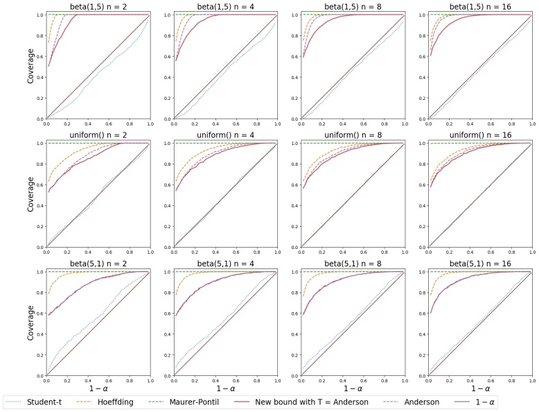
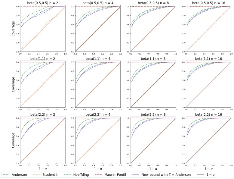
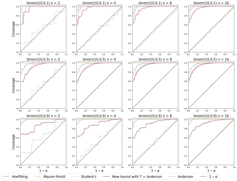
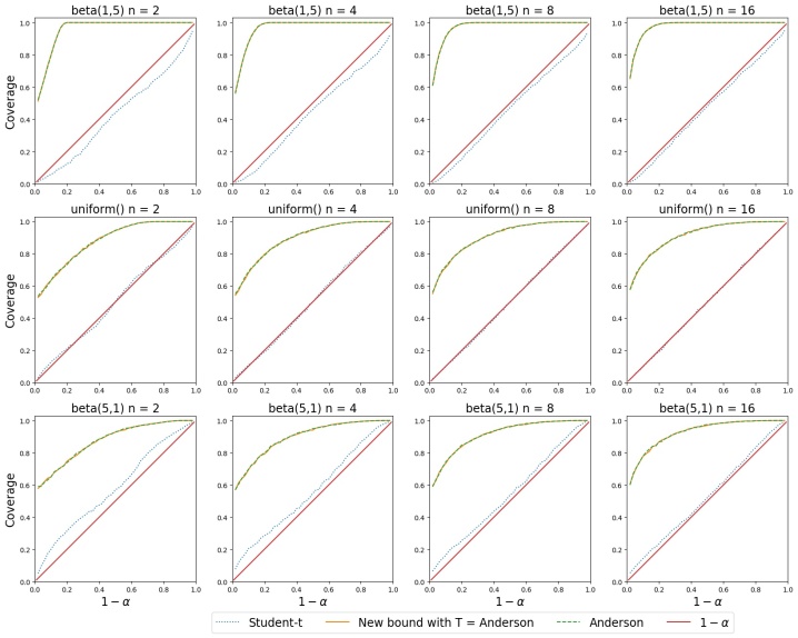
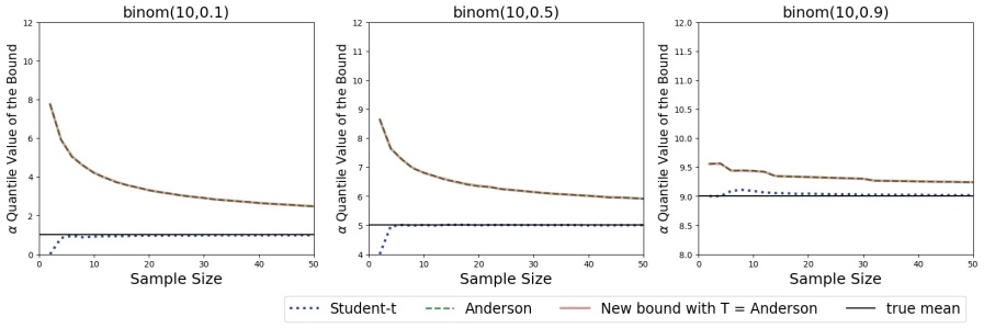
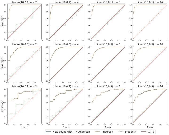
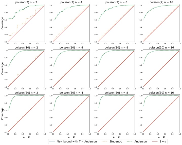
All the experiments confirm that our bound has guaranteed coverage and is equal to or tighter than Anderson’s and Hoeffding’s.

From the experiments, our upper bound performs the best in distributions that are skewed right (respectively, our lower bound will perform the best in distributions that are skewed left), when we know a tight lower bound and upper bound of the support.

Appendix B Discussion on Section 1: Skewed Sample Mean Distribution with $n=80$

In this section, as noted in Section 1, we show a log-normal distribution where the sample mean distribution is visibly skewed when $n=80$ (Figure 11). Student’s $t$ is not a good candidate in this case because the sample mean distribution is not approximately normal. This example is a variation on the one provided by Frost (2021).

While the log-normal distribution is an extreme example of skew, this example illustrates the danger of assuming the validity of arbitrary thresholds on the sample size, such as the traditional threshold of $n=30$, for using the Student’s $t$ method. Clearly there are cases where such a threshold, and even much larger thresholds, are not adequate.

Figure 11: The PDFs of $lognorm(0,1)$ and the sample mean distribution of $lognorm(0,1)$. The sample mean distribution of $lognorm(0,1)$ is visibly skewed when the sample size $n=80$.

Appendix C Proof of Section 2.1.2

We restate the lemma and theorem statements for convenience.

Lemma C.1 (Lemma 2.2).

Let $X$ be a random variable with CDF $F$ and $Y\overset{\underset{\mathrm{def}}{}}{=}F(X)$, known as the probability integral transform of $X$. Let $U$ be a uniform random variable on $[0,1]$. Then for any $0\leq y\leq 1$,

$$\mathbb{P}(Y\leq y)\leq\mathbb{P}(U\leq y).$$ (52)

If $F$ is continuous, then $Y$ is uniformly distributed on $(0,1)$.

Proof.

Let $F^{-1}(y)=\inf\{x:F(x)\geq y\}$ for $0<y<1$ and $U$ be an uniform random variable on $(0,1)$. Since $F$ is non-decreasing and right-continuous, $F(F^{-1}(y))\geq y$ . By Angus (1994), $F^{-1}(U)$ has CDF $F$. For $0<y<1$, then:

$$\mathbb{P}(Y\leq y) =\mathbb{P}(F(X)\leq y)$$ (53)

$$=\mathbb{P}(F(F^{-1}(U))\leq y)$$ (54)

$$\leq\mathbb{P}(U\leq y)$$ (55)

$$=y.$$ (56)

If $F$ is continuous, Angus (1994) shows that $Y$ is uniformly distributed on $(0,1)$. ∎

Lemma C.2 (Lemma 2.3).

Let $F$ and $G_{\mathbf{x},\boldsymbol{\ell}}$ be two CDF functions such that $\forall x\in\mathcal{R}$, $F(x)\geq G_{\mathbf{x},\boldsymbol{\ell}}(x)$. Let $\mu_{F}$ and $\mu_{G}$ denote the means of $F$ and $G_{\mathbf{x},\boldsymbol{\ell}}$. Then:

$$\mu_{F}\leq\mu_{G}.$$ (57)

Proof.

Let $x_{(0)}\overset{\underset{\mathrm{def}}{}}{=}-\infty$ and $x_{(n+1)}\overset{\underset{\mathrm{def}}{}}{=}s_{D}$. Then:

$$\mu_{F} =\int x\;dF(x)$$ (58)

$$=\sum_{i=1}^{n+1}\int_{x_{(i-1)}}^{x_{(i)}}x\;dF(x)$$ (59)

$$\leq\sum_{i=1}^{n+1}\int_{x_{(i-1)}}^{x_{(i)}}x_{(i)}\;dF(x)$$ (60)

$$=\sum_{i=1}^{n+1}x_{(i)}(F(x_{(i)})-F(x_{(i-1)}))$$ (61)

$$=s_{D}-\sum_{i=1}^{n}F(x_{(i)})(x_{(i+1)}-x_{(i)})$$ (62)

$$\leq s_{D}-\sum_{i=1}^{n}G(x_{(i)})(x_{(i+1)}-x_{(i)})$$ (63)

$$=\mu_{G}$$ (64)

∎

Lemma C.3 (Lemma 2.4).

Let $\mathbf{Z}$ be a random sample of size $n$ from $F$. Let $\mathbf{U}=U_{1},...,U_{n}$ be a sample of size $n$ from the continuous uniform distribution on $[0,1]$. For any function $T:D^{n}\rightarrow R$ and any $\mathbf{x}\in D^{n}$,

$$\mathbb{P}_{\mathbf{Z}}(T(\mathbf{Z})\leq T(\mathbf{x}))\leq\mathbb{P}_{\mathbf{U}}(b(\mathbf{x},\mathbf{U})\geq\mu).$$ (65)

Proof.

Let $\cup$ denote the union of events and $\{\}$ denote an event. Let $\mathbf{Z}$ be a sample from $F$. Then for any sample $\mathbf{x}$:

$$\mathbb{P}_{\mathbf{Z}}(T(\mathbf{Z})\leq T(\mathbf{x}))$$ (66)

$$=\mathbb{P}_{\mathbf{Z}}(\mathbf{Z}\in\mathbb{S}(\mathbf{x}))$$ (67)

$$=\mathbb{P}_{\mathbf{Z}}(\cup_{\mathbf{y}\in\mathbb{S}(\mathbf{x})}\{\mathbf{Z}=\mathbf{y}\})$$ (68)

$$\leq\mathbb{P}_{\mathbf{Z}}(\cup_{\mathbf{y}\in\mathbb{S}(\mathbf{x})}\mathbf{Z}\preceq\mathbf{y})\text{ because $\mathbf{Z}=\mathbf{y}$ implies $\mathbf{Z}\preceq\mathbf{y}$ }$$ (69)

$$\leq\mathbb{P}_{\mathbf{Z}}(\cup_{\mathbf{y}\in\mathbb{S}(\mathbf{x})}\{F(\mathbf{Z})\preceq F(\mathbf{y})\})$$ (70)

because $F$ is non-decreasing, so $Z_{(i)}\leq y_{(i)}$ implies $F(Z_{(i)})\leq F(y_{(i)})$. Let $U_{1},\cdots,U_{n}$ be $n$ samples from the uniform distribution on $(0,1)$. From Lemma 2.2, for any $u\in(0,1)$, $\mathbb{P}(F(Z_{i})\leq u)\leq\mathbb{P}(U_{i}\leq u)$. Therefore

$$\mathbb{P}_{\mathbf{Z}}(\cup_{\mathbf{y}\in\mathbb{S}(\mathbf{x})}\{F(\mathbf{Z})\preceq F(\mathbf{y})\})$$ (71)

$$\leq\mathbb{P}_{\mathbf{U}}(\cup_{\mathbf{y}\in\mathbb{S}(\mathbf{x})}\{\mathbf{U}\preceq F(\mathbf{y})\}).$$ (72)

Recall that $m_{D}(\mathbf{y},\mathbf{U})=s_{D}-\sum_{i=1}^{n}U_{(i)}(y_{(i+1)}-y_{(i)})$ where $\forall i,y_{(i+1)}-y_{(i)}\geq 0$. Therefore if $\forall i,U_{(i)}\leq F(y_{(i)})$ then $m_{D}(\mathbf{y},\mathbf{U})\geq m_{D}(\mathbf{y},F(\mathbf{y}))$:

$$\mathbb{P}_{\mathbf{U}}(\cup_{\mathbf{y}\in\mathbb{S}(\mathbf{x})}\{\mathbf{U}\preceq F(\mathbf{y})\})$$ (73)

$$\leq\mathbb{P}_{\mathbf{U}}(\cup_{\mathbf{y}\in\mathbb{S}(\mathbf{x})}\{m_{D}(\mathbf{y},\mathbf{U})\geq m_{D}(\mathbf{y},F(\mathbf{y}))\}),\text{by Lemma~{}\ref{lem:helper2}}$$ (74)

$$\leq\mathbb{P}_{\mathbf{U}}(\cup_{\mathbf{y}\in\mathbb{S}(\mathbf{x})}\{m_{D}(\mathbf{y},\mathbf{U})\geq\mu\}),\text{by Lemma~{}\ref{lem:helper2}}$$ (75)

$$\leq\mathbb{P}_{\mathbf{U}}(\sup_{\mathbf{y}\in\mathbb{S}(\mathbf{x})}m_{D}(\mathbf{y},\mathbf{U})\geq\mu)$$ (76)

$$=\mathbb{P}_{\mathbf{U}}(b(\mathbf{x},\mathbf{U})\geq\mu)$$ (77)

The inequality in Eq. 76 is because if there exists $\mathbf{y}\in\mathbb{S}(\mathbf{x})$ such that $m_{D}(\mathbf{y},\mathbf{U})\geq\mu$, then $\sup_{\mathbf{y}\in\mathbb{S}(\mathbf{x})}m_{D}(\mathbf{y},\mathbf{U})\geq\mu$. Therefore the event $\cup_{\mathbf{y}\in\mathbb{S}(\mathbf{x})}\{m_{D}(\mathbf{y},\mathbf{U})\geq\mu\}$ is a subset of the event $\sup_{\mathbf{y}\in\mathbb{S}(\mathbf{x})}m_{D}(\mathbf{y},\mathbf{U})\geq\mu$, and Eq. 76 follows.

From Eqs. 70, 72 and Eq. 77:

$$\mathbb{P}_{\mathbf{Z}}(T(\mathbf{Z})\leq T(\mathbf{x}))\quad\leq\quad\mathbb{P}_{\mathbf{U}}(b(\mathbf{x},\mathbf{U})\geq\mu).$$ (78)

∎

Appendix D Discussion on Section 3: Monte Carlo Convergence

In Section 3, we discussed the use of Monte Carlo sampling of the induced mean function $b(\mathbf{x},\mathbf{U})$ via sampling of the uniform random variable $U$, to approximate the $1-\alpha$ quantile of $b(\mathbf{x},\mathbf{U})$. Let $\hat{q}_{\ell}$ denote the output of the Monte Carlo algorithm (Algorithm 1) using $\ell$ Monte Carlo samples. In this section we show that our estimator converges to the true quantile as the number of Monte Carlo samples grows, and, given a desired threshold $\epsilon$, we can compute an upper bound at most $Q(1-\alpha,b(\mathbf{x},\mathbf{U}))+\epsilon$ with guaranteed coverage.

Theorem D.1.

Let $\epsilon>0$. Let $\gamma=\min\left(\alpha,\left(\frac{\epsilon}{3(s_{D}-\sup_{\mathbf{z}\in\mathbb{S}(\mathbf{x}))}z_{(1)})}\right)^{n}\right)$. Use $\ell=\left\lceil\frac{-\ln(\gamma/2)}{2}\left(\frac{3(s_{D}-\sup_{\mathbf{z}\in\mathbb{S}(\mathbf{x})}z_{(1)})}{\epsilon}\right)^{n}\right\rceil$ Monte Carlo samples to compute $Q(1-\alpha+\gamma,b(\mathbf{x},\mathbf{U}))$ using Algorithm 1. Let $\hat{q}_{\ell}$ be the output of the algorithm. We output $\hat{q}_{\ell}+\epsilon/3$ as the final estimator.

Then with probability at least $1-\alpha$:

$$\mu\leq\hat{q}_{\ell}+\epsilon/3\leq Q(1-\alpha,b(\mathbf{x},\mathbf{U}))+\epsilon.$$ (79)

To prove Theorem D.1, we first show some lemmas.

The Monte Carlo approximation error is quantified in the following lemma due to Serfling (1980). Let $F(m-)\overset{\underset{\mathrm{def}}{}}{=}\lim_{x\rightarrow m^{-}}F(x)$.

Lemma D.2 (Theorem 2.3.2 in Serfling (1980)).

Let $0<p<1$. If $Q(p,M)$ is the unique solution $m$ of $F(m-)\leq p\leq F(m)$, then for every $\epsilon>0$,

$$\mathbb{P}(|\mathbf{M}_{\lceil pl\rceil}-Q(p,M)|>\epsilon)\leq 2e^{-2l\delta},$$ (80)

where $\mathbf{M}_{k}$ denotes the $k$-th order statistic of the sample $\mathbf{M}$ and

$$\delta=\min\left(p-F(Q(p,M)-\epsilon),F(Q(p,M)+\epsilon)-p\right).$$

Note that when the condition that $Q(p,M)$ is the unique solution $m$ of $F(m-)\leq p\leq F(m)$ is satisfied, $\delta>0$. Let $M\overset{\underset{\mathrm{def}}{}}{=}b_{D,T}(\mathbf{x},\mathbf{U})\in[0,1]$. In Lemma D.3 we will show that the CDF of $M$ satisfies the condition in Lemma D.2. Therefore the error incurred by computing the bound via Monte Carlo sampling can be decreased to an arbitrarily small value by choosing a large enough number of Monte Carlo samples $l$. The Monte Carlo estimation of $b^{\alpha}_{D^{+},T}(\mathbf{x})$ where $D^{+}=[0,1]$ is presented in Algorithm 1.

We will show that for any $\mathbf{x}$, for any $T$, for any $p\in(0,1)$, $F_{M}(m-)\leq p\leq F_{M}(m)$ has a unique solution by showing that for any $\mathbf{x}$ and $T$, $F_{M}$ is strictly increasing on its support. To do so, for any $c_{1},c_{2}$ in the support such that $c_{1}<c_{2}$ we will show that

$$F_{M}(c_{2})-F_{M}(c_{1})>0.$$ (81)

Lemma D.3.

Let $M\overset{\underset{\mathrm{def}}{}}{=}b(\mathbf{x},\mathbf{U})$. Let $F_{M}$ be the CDF of $M$.

For any $\mathbf{x}$, for any scalar function $T$, either:

1. $M$ is a constant, or

2. For any $c_{1},c_{2}$ such that $0\leq c_{1}<c_{2}\leq 1$,

   $$F_{M}(c_{2})-F_{M}(c_{1})\geq\left(\frac{c_{2}-c_{1}}{s_{D}-\sup_{\mathbf{z}\in\mathbb{S}(\mathbf{x})}z_{(1)}}\right)^{n}>0.$$ (82)

Proof.

Recall the definition of the induced mean as

$$b(\mathbf{x},\boldsymbol{\ell}) =\sup_{\mathbf{z}\in\mathbb{S}(\mathbf{x})}\sum_{i=1}^{n+1}z_{(i)}(\ell_{(i)}-\ell_{(i-1)}),$$ (83)

$$=\sup_{\mathbf{z}\in\mathbb{S}(\mathbf{x})}s_{D}-\sum_{i=1}^{n}\ell_{(i)}(z_{(i+1)}-z_{(i)}),$$ (84)

where $\ell_{(0)}\overset{\underset{\mathrm{def}}{}}{=}0$, $\ell_{(n+1)}\overset{\underset{\mathrm{def}}{}}{=}1$ and $z_{(n+1)}\overset{\underset{\mathrm{def}}{}}{=}s_{D}$.

We now find the support of $M$. Let $\phi\overset{\underset{\mathrm{def}}{}}{=}\sup_{\mathbf{z}\in\mathbb{S}(\mathbf{x})}z_{(1)}$. We will show that for any $\mathbf{u}$ where $0\leq u_{i}\leq 1$, we have $\phi\leq b(\mathbf{x},\mathbf{u})\leq s_{D}$, and therefore the support of $M$ is a subset of $[\phi,s_{D}]$. We have

$$b(\mathbf{x},\mathbf{u}) =\sup_{\mathbf{z}\in\mathbb{S}(\mathbf{x})}s_{D}-\sum_{i=1}^{n}u_{(i)}(z_{(i+1)}-z_{(i)})$$ (85)

$$\leq\sup_{\mathbf{z}\in\mathbb{S}(\mathbf{x})}s_{D}-\sum_{i=1}^{n}0(z_{(i+1)}-z_{(i)})$$ (86)

$$=s_{D}.$$ (87)

Similarly we have

$$b(\mathbf{x},\mathbf{u}) =\sup_{\mathbf{z}\in\mathbb{S}(\mathbf{x})}s_{D}-\sum_{i=1}^{n}u_{(i)}(z_{(i+1)}-z_{(i)})$$ (88)

$$\geq\sup_{\mathbf{z}\in\mathbb{S}(\mathbf{x})}s_{D}-\sum_{i=1}^{n}1(z_{(i+1)}-z_{(i)})$$ (89)

$$=\sup_{\mathbf{z}\in\mathbb{S}(\mathbf{x})}s_{D}-(z_{(n+1)}-z_{(1)})$$ (90)

$$=\sup_{\mathbf{z}\in\mathbb{S}(\mathbf{x})}z_{(1)}$$ (91)

$$=\phi.$$ (92)

Therefore $M=b(\mathbf{x},\mathbf{U})\in[\phi,s_{D}]$. We consider two cases: where $\phi=s_{D}$ and where $\phi<s_{D}$.

Case $1$: $\phi=s_{D}$.

Then for all $i$, $\sup_{\mathbf{z}\in\mathbb{S}(\mathbf{x})}z_{(i)}\geq\phi=s_{D}$. Since $z_{(i)}\leq s_{D}$, we have for all $i$, $\sup_{\mathbf{z}\in\mathbb{S}(\mathbf{x})}z_{(i)}=s_{D}$. Therefore

$$b(\mathbf{x},\boldsymbol{\ell}) =\sup_{\mathbf{z}\in\mathbb{S}(\mathbf{x})}\sum_{i=1}^{n+1}z_{(i)}(\ell_{(i)}-\ell_{(i-1)})$$ (93)

$$=\sum_{i=1}^{n+1}s_{D}(\ell_{(i)}-\ell_{(i-1)})$$ (94)

$$=s_{D}.$$ (95)

Therefore $M=b(\mathbf{x},\mathbf{U})$ is a constant $s_{D}$, and the $1-\alpha$ quantile of $M$ is $s_{D}$.

Case $2$: $\phi<s_{D}$.

Let $c_{1},c_{2}\in\mathcal{R}$ be such that $\phi\leq c_{1}<c_{2}\leq s_{D}$. We will now show that

$$F_{M}(c_{2})-F_{M}(c_{1})>0.$$ (96)

Let $v\overset{\underset{\mathrm{def}}{}}{=}\frac{s_{D}-c_{2}}{s_{D}-\phi}$ and $w\overset{\underset{\mathrm{def}}{}}{=}\frac{s_{D}-c_{1}}{s_{D}-\phi}$. If $\phi\leq c_{1}<c_{2}\leq s_{D}$ then $v<w$ and $v,w\in[0,1]$.

Let $\mathbf{v}\overset{\underset{\mathrm{def}}{}}{=}(v_{1},\cdots,v_{n})$ and $\mathbf{w}\overset{\underset{\mathrm{def}}{}}{=}(w_{1},\cdots,w_{n})$ where $\forall i,v_{i}=v$ and $w_{i}=w$. Then

$$b(\mathbf{x},\mathbf{v}) =\sup_{\mathbf{z}\in\mathbb{S}(\mathbf{x})}\sum_{i=1}^{n+1}z_{(i)}(v_{(i)}-v_{(i-1)})$$ (97)

$$=\sup_{\mathbf{z}\in\mathbb{S}(\mathbf{x})}z_{(n+1)}(v_{(n+1)}-v_{(n)})+z_{(1)}(v_{(1)}-v_{(0)})$$ (98)

$$=\sup_{\mathbf{z}\in\mathbb{S}(\mathbf{x})}s_{D}(1-v)+z_{(1)}(v-0)$$ (99)

$$=\sup_{\mathbf{z}\in\mathbb{S}(\mathbf{x})}s_{D}-(s_{D}-z_{(1)})\frac{s_{D}-c_{2}}{s_{D}-\phi}$$ (100)

$$=s_{D}-(s_{D}-\phi)\frac{s_{D}-c_{2}}{s_{D}-\phi}\text{ because $\frac{s_{D}-c_{2}}{s_{D}-\phi}\geq 0$}$$ (101)

$$=c_{2}.$$ (102)

Similarly,

$$b(\mathbf{x},\mathbf{w}) =\sup_{\mathbf{z}\in\mathbb{S}(\mathbf{x})}\sum_{i=1}^{n+1}z_{(i)}(w_{(i)}-w_{(i-1)})$$ (103)

$$=\sup_{\mathbf{z}\in\mathbb{S}(\mathbf{x})}z_{(n+1)}(w_{(n+1)}-w_{(n)})+z_{(1)}(w_{(1)}-w_{(0)})$$ (104)

$$=\sup_{\mathbf{z}\in\mathbb{S}(\mathbf{x})}s_{D}(1-w)+z_{(1)}(w-0)$$ (105)

$$=\sup_{\mathbf{z}\in\mathbb{S}(\mathbf{x})}s_{D}-(s_{D}-z_{(1)})\frac{s_{D}-c_{1}}{s_{D}-\phi}$$ (106)

$$=s_{D}-(s_{D}-\phi)\frac{s_{D}-c_{1}}{s_{D}-\phi}\text{ because $\frac{s_{D}-c_{1}}{s_{D}-\phi}\geq 0$}$$ (107)

$$=c_{1}.$$ (108)

Since $b(\mathbf{x},\mathbf{u})$ is constructed from a linear function of $\mathbf{u}$ with non-positive coefficients, for any $\mathbf{u}$ such that $v\leq u_{(1)}\leq\cdots\leq u_{(n)}<w$ we have:

$$b(\mathbf{x},\mathbf{w})<b(\mathbf{x},\mathbf{u})\leq b(\mathbf{x},\mathbf{v}),$$ (109)

which is equivalent to:

$$c_{1}<b(\mathbf{x},\mathbf{u})\leq c_{2}.$$ (110)

So we have $v\leq u_{(1)}\leq\cdots\leq u_{(n)}<w$ implies $c_{1}<b(\mathbf{x},\mathbf{u})\leq c_{2}$. Therefore for any $c_{1},c_{2}$ such that $\phi\leq c_{1}<c_{2}\leq s_{D}$:

$$F_{M}(c_{2})-F_{M}(c_{1})$$ (111)

$$=\mathbb{P}(c_{1}<M\leq c_{2})$$ (112)

$$=\mathbb{P}_{\mathbf{U}}(c_{1}<b(\mathbf{x},\mathbf{U})\leq c_{2})$$ (113)

$$\geq\mathbb{P}_{\mathbf{U}}(v\leq U_{(1)}\leq\cdots\leq U_{(n)}<w)$$ (114)

$$=\mathbb{P}_{\mathbf{U}}(~{}\forall i,1\leq i\leq n:v\leq U_{i}<w)$$ (115)

$$=(w-v)^{n}$$ (116)

$$=\left(\frac{c_{2}-c_{1}}{s_{D}-\phi}\right)^{n}$$ (117)

$$>0\text{ because $c_{1}<c_{2}$}.$$ (118)

Since the support of $M$ is in $[\phi,s_{D}]$ we have that $F_{M}$ is strictly increasing on the support. ∎

In summary, the Monte Carlo estimate of our bound will converge to the correct value as the number of samples grows.

Now we prove Theorem D.1.

Proof of Theorem D.1.

To simplify the notation, we use $Q(\alpha)$ to denote $Q(\alpha,M)$. From Lemma D.3, since $F_{M}$ is strictly increasing on the support, for $\gamma$ such that $0<\gamma\leq\alpha$, $Q(1-\alpha)<Q(1-\alpha+\gamma)$ and:

$$\gamma=F(Q(1-\alpha),Q(1-\alpha+\gamma))\geq\left(\frac{Q(1-\alpha+\gamma)-Q(1-\alpha)}{s_{D}-\sup_{\mathbf{z}\in\mathbb{S}(\mathbf{x})}z_{(1)}}\right)^{n}.$$ (119)

Therefore, letting $\gamma=\min\left(\alpha,\left(\frac{\epsilon}{3(s_{D}-\sup_{\mathbf{z}\in\mathbb{S}(\mathbf{x}))}z_{(1)})}\right)^{n}\right)$ we have that

$$Q(1-\alpha+\gamma) \leq Q(1-\alpha)+\gamma^{1/n}(s_{D}-\sup_{\mathbf{z}\in\mathbb{S}(\mathbf{x})}z_{(1)})$$ (120)

$$\leq Q(1-\alpha)+\epsilon/3.$$ (121)

Let $p\overset{\underset{\mathrm{def}}{}}{=}1-\alpha+\gamma$. From Lemma D.2 and Lemma D.3,

$$\mathbb{P}(|\hat{q}_{\ell}-Q(p)|>\epsilon/3)\leq 2e^{-2l\delta},$$ (122)

where

$$\delta =\min\left(p-F(Q(p)-\epsilon/3),F(Q(p)+\epsilon/3)-p\right)$$ (123)

$$=\min\left(F(Q(p)-\epsilon/3,Q(p)),F(Q(p),Q(p)+\epsilon/3)\right)$$ (124)

$$\geq\left(\frac{\epsilon}{3(s_{D}-\sup_{\mathbf{z}\in\mathbb{S}(\mathbf{x})}z_{(1)})}\right)^{n}.$$ (125)

Therefore letting $\ell=\left\lceil\frac{-\ln(\gamma/2)}{2}\left(\frac{3(s_{D}-\sup_{\mathbf{z}\in\mathbb{S}(\mathbf{x})}z_{(1)})}{\epsilon}\right)^{n}\right\rceil$,

$$\mathbb{P}(|\hat{q}_{\ell}-Q(1-\alpha+\gamma)|>\epsilon/3) \leq 2e^{-2l\left(\frac{\epsilon}{3(s_{D}-\sup_{\mathbf{z}\in\mathbb{S}(\mathbf{x})}z_{(1)})}\right)^{n}}$$ (126)

$$\leq\gamma.$$ (127)

Since $\mathbb{P}(Q(1-\alpha+\gamma)<\mu)\leq\alpha-\gamma$, using the union bound we have

$$\mathbb{P}(|\hat{q}_{\ell}-Q(1-\alpha+\gamma)|>\epsilon/3\text{ OR }Q(1-\alpha+\gamma)<\mu) \leq\gamma+\alpha-\gamma$$ (128)

$$=\alpha.$$ (129)

And therefore,

$$1-\alpha \leq\mathbb{P}(|\hat{q}_{\ell}-Q(1-\alpha+\gamma)|\leq\epsilon/3\text{ AND }Q(1-\alpha+\gamma)\geq\mu)$$ (130)

$$\leq\mathbb{P}(Q(1-\alpha+\gamma)\leq\hat{q}_{\ell}+\epsilon/3\leq Q(1-\alpha+\gamma)+2\epsilon/3\text{ AND }Q(1-\alpha+\gamma)\geq\mu)$$ (131)

$$\leq\mathbb{P}(\mu\leq\hat{q}_{\ell}+\epsilon/3\leq Q(1-\alpha+\gamma)+2\epsilon/3)$$ (132)

$$\leq\mathbb{P}(\mu\leq\hat{q}_{\ell}+\epsilon/3\leq Q(1-\alpha)+\epsilon)\text{ from Eq.~{}\ref{eq:quantile_shift}}.$$ (133)

∎

Appendix E Discussion on Section 4

We discuss the case when the distribution is Bernoulli in Section E.1, and present the proofs of Section 4.2 in Section E.2. In Section E.3 we show that our bound is equal to Anderson’s when $T$ is Anderson’s bound and the lower bound of the support is $-\infty$, and could be better than Anderson’s when $T$ is Anderson’s bound and the lower bound of the support is finite and tight.

E.1 Special Case: Bernoulli Distribution

When we know that $D=\{0,1\}$, the distribution is Bernoulli. If we choose $T$ to be the sample mean, we will show that our bound becomes the same as the Clopper-Pearson confidence bound for binomial distributions (Clopper & Pearson, 1934).

If $\mathbf{x},\mathbf{z}\in\{0,1\}^{n}$ and $T(\mathbf{z})\leq T(\mathbf{x})$ then $m(\mathbf{z},\mathbf{u})\leq m(\mathbf{x},\mathbf{u})$. Therefore for any $\mathbf{u}\in[0,1]^{n}$,

$$b_{D,T}(\mathbf{x},\mathbf{u})=\sup_{\mathbf{z}\in\{0,1\}^{n}:T(\mathbf{z})\leq T(\mathbf{x})}m_{D}(\mathbf{z},\mathbf{u})=m_{D}(\mathbf{x},\mathbf{u}).$$ (134)

Let $p_{\mathbf{x}}$ be the number of $0$’s in $\mathbf{x}$. Therefore the bound becomes the $1-\alpha$ quantile of $m_{D}(\mathbf{x},\mathbf{U})$ where

$$m_{D}(\mathbf{x},\mathbf{U})=1-\sum_{i=1}^{n}U_{(i)}(x_{(i+1)}-x_{(i)})=1-U_{(p_{\mathbf{x}})}.$$ (135)

Therefore the bound is the $1-\alpha$ quantile of $1-U_{(p_{\mathbf{x}})}$. Then

$$\mathbb{P}(U_{(p_{\mathbf{x}})}\leq 1-b^{\alpha}(\mathbf{x}))=\mathbb{P}(1-U_{(p_{\mathbf{x}})}\geq b^{\alpha}(\mathbf{x}))=\alpha.$$ (136)

Let $\beta(i,j)$ denote a beta distribution with parameters $i$ and $j$. We use the fact that the order statistics of a uniform distribution are beta-distributed. Since $U_{(p_{\mathbf{x}})}\sim\beta(p_{\mathbf{x}},n+1-p_{\mathbf{x}})$, we have $1-U_{(p_{\mathbf{x}})}\sim\beta(n-p_{\mathbf{x}}+1,p_{\mathbf{x}})$

$$b^{\alpha}(\mathbf{x})=Q(1-\alpha,\beta(n-p_{\mathbf{x}}+1,p_{\mathbf{x}})).$$ (137)

This is the same as the Clopper-Pearson upper confidence bound for binomial distributions.

E.2 Proof of Section 4.2

Lemma E.1 (Lemma 4.1).

Let $\mathbf{X}=(X_{1},\cdots,X_{n})$ be a sample of size $n$ from a distribution with mean $\mu$. Let $\boldsymbol{\ell}\in[0,1]^{n}$. If $G_{\mathbf{X},\boldsymbol{\ell}}$ is a $(1-\alpha)$ lower confidence bound for the CDF then

$$\mathbb{P}_{\mathbf{X}}(m(\mathbf{X},\boldsymbol{\ell})\geq\mu)\geq 1-\alpha.$$ (138)

Proof.

If $\forall y\in\mathcal{R},F(y)\geq G_{\mathbf{X},\boldsymbol{\ell}}(y)$ then

$$\forall i:1\leq i\leq n,F(X_{(i)})\geq\ell_{(i)}.$$ (139)

Recall that $m_{D}(\mathbf{X},\boldsymbol{\ell})=s_{D}-\sum_{i=1}^{n}\ell_{(i)}(z_{(i+1)}-z_{(i)})$. Therefore if $\forall i:1\leq i\leq n,~{}F(X_{(i)})\geq\ell_{(i)}$ then $m(\mathbf{X},\boldsymbol{\ell})\geq m(\mathbf{X},F(\mathbf{X}))$.

From Lemma 2.3, $m(\mathbf{X},F(\mathbf{X}))\geq\mu$. Therefore $m(\mathbf{X},\boldsymbol{\ell})\geq\mu$. And hence, finally,

$$\mathbb{P}(m(\mathbf{X},\boldsymbol{\ell})\geq\mu) \geq\mathbb{P}_{\mathbf{X}}\left(\forall y\in\mathcal{R},F(y)\geq G_{\mathbf{X},\boldsymbol{\ell}}(y)\right)$$ (140)

$$=1-\alpha.$$ (141)

∎

We now show that if $G_{\mathbf{X},\boldsymbol{\ell}}$ (Figure 1(a)) is a lower confidence bound, then the order statistics of $\boldsymbol{\ell}$ are element-wise smaller than the order statistics of a sample of size $n$ from the uniform distribution with high probability:

Lemma E.2.

Let $\mathbf{U}=U_{1},...,U_{n}$ be a sample of size $n$ from the continuous uniform distribution on $[0,1]$. Let $\boldsymbol{\ell}\in[0,1]^{n}$ and $\alpha\in(0,1)$. If $\mathcal{D}^{+}$ is continous and $G_{\mathbf{X},\boldsymbol{\ell}}$ is a $(1-\alpha)$ lower confidence bound for the CDF then:

$$\mathbb{P}_{\mathbf{U}}(~{}\forall i:1\leq i\leq n,U_{(i)}\geq\ell_{(i)})\geq 1-\alpha.$$ (142)

Proof.

Let $K$ be the CDF of a distribution such that $K$ is continuous and strictly increasing on $\mathcal{D}^{+}$ (since $\mathcal{D}^{+}$ is continuous, $K$ exists). Let $\mathbf{X}=(X_{1},\cdots,X_{n})$ be a sample of size $n$ from the distribution with CDF $K$. By Lemma 2.2, $K(X)$ is uniformly distributed on $[0,1]$.

By the definition of $G_{\mathbf{X},\boldsymbol{\ell}}$, if $~{}\forall x\in C,K(y)\geq G_{\mathbf{X},\boldsymbol{\ell}}(y)$ then:

$$K(y)\geq 0, \text{ if }y<X_{(1)}$$ (143)

$$K(y)\geq\ell_{(i)}, \text{ if }X_{(i)}\leq y<X_{(i+1)}$$ (144)

$$K(y)\geq 1, \text{ if }y\geq s_{C}.$$ (145)

which is equivalent to:

$$~{}\forall i:1\leq i\leq n,K(y)\geq\ell_{(i)}, \text{ if }X_{(i)}\leq y<X_{(i+1)}.$$ (146)

Since $K(y)$ is non-decreasing, this is equivalent to:

$$~{}\forall i:1\leq i\leq n,K(X_{(i)})\geq\ell_{(i)}$$ (147)

Since $G_{\mathbf{X},\boldsymbol{\ell}}$ is a lower confidence bound,

$$1-\alpha \leq\mathbb{P}_{\mathbf{X}}(~{}\forall y\in\mathcal{R},K(y)\geq G_{\mathbf{X},\boldsymbol{\ell}}(y))$$ (148)

$$=\mathbb{P}_{\mathbf{X}}(\forall i:1\leq i\leq n,K(X_{(i)})\geq\ell_{(i)})$$ (149)

$$=\mathbb{P}_{\mathbf{U}}(\forall i:1\leq i\leq n,U_{(i)}\geq\ell_{(i)})\text{ by Lemma~{}\ref{lem:CDF_vs_U}}.$$ (150)

∎

To prove Theorem 4.3, we prove the more general version where $G_{\mathbf{X},\boldsymbol{\ell}}$ is a (possibly not exact) lower confidence bound for the CDF.

Theorem E.3.

Let $\boldsymbol{\ell}\in[0,1]^{n}$. Let $D^{+}=[-\infty,b]$. If $G_{\mathbf{X},\boldsymbol{\ell}}$ is a $1-\alpha$ lower confidence bound for the CDF, then for any sample size $n$, for all sample values $\mathbf{x}\in D^{n}$ and all $\alpha\in(0,1)$, using $T(\mathbf{x})=m_{{D^{+}}}(\mathbf{x},\boldsymbol{\ell})$ to compute $b^{\alpha}_{{D^{+}},T}(\mathbf{x})$ yields:

$$b^{\alpha}_{{D^{+}},T}(\mathbf{x})\leq m_{{D^{+}}}(\mathbf{x},\boldsymbol{\ell}).$$ (151)

Proof.

Since $G_{\mathbf{X},\boldsymbol{\ell}}$ is a lower confidence bound for the CDF $F$, from Lemma E.2,

$$\mathbb{P}(\forall i,U_{(i)}\geq\ell_{(i)})\geq 1-\alpha.$$ (152)

First we note that

$$b_{{D^{+}},T}(\mathbf{x},\boldsymbol{\ell}) =\sup_{\mathbf{y}:\mathbf{y}\in\mathbb{S}_{{D^{+}},T}(\mathbf{x})}m_{{D^{+}}}(\mathbf{y},\boldsymbol{\ell})$$ (153)

$$=\sup_{m_{{D^{+}}}(\mathbf{y},\boldsymbol{\ell})\leq m_{{D^{+}}}(\mathbf{x},\boldsymbol{\ell})}m_{{D^{+}}}(\mathbf{y},\boldsymbol{\ell})$$ (154)

$$=m_{{D^{+}}}(\mathbf{x},\boldsymbol{\ell}).$$ (155)

Recall that $b_{{D^{+}},T}^{\alpha}(\mathbf{x})$ is the $1-\alpha$ quantile of $b_{{D^{+}},T}(\mathbf{x},\mathbf{U})$. In order to show that $b_{{D^{+}},T}^{\alpha}(\mathbf{x})\leq b_{{D^{+}},T}(\mathbf{x},\boldsymbol{\ell})$, we will show that

$$\mathbb{P}(b_{{D^{+}},T}(\mathbf{x},\mathbf{U})\leq b_{{D^{+}},T}(\mathbf{x},\boldsymbol{\ell}))\geq 1-\alpha.$$ (156)

Recall that $b_{{D^{+}},T}(\mathbf{x},\mathbf{U})=\sup_{\mathbf{y}\in\mathbb{S}_{T}(\mathbf{x})}t_{{D^{+}}}-\sum_{i=1}^{n}U_{(i)}(x_{(i+1)}-x_{(i)})$. Then if $~{}\forall i,U_{(i)}\geq\ell_{(i)}$ then $b_{{D^{+}},T}(\mathbf{x},\mathbf{U})\leq b_{{D^{+}},T}(\mathbf{x},\boldsymbol{\ell})$. Therefore,

$$\mathbb{P}(b_{{D^{+}},T}(\mathbf{x},\mathbf{U})\leq b_{{D^{+}},T}(\mathbf{x},\boldsymbol{\ell}))$$ (157)

$$\geq\mathbb{P}(\forall i,U_{(i)}\geq\ell_{(i)})$$ (158)

$$\geq 1-\alpha,\text{ by Lemma~{}\ref{lem:lower_bound_cdf}}.$$ (159)

∎

We can now show the comparison with Anderson’s bound and Hoeffding’s bound.

Theorem E.4 (Theorem 4.3).

Let $\boldsymbol{\ell}\in[0,1]^{n}$ be a vector such that $G_{\mathbf{X},\boldsymbol{\ell}}$ is an exact $(1-\alpha)$ lower confidence bound for the CDF.

Let $D^{+}=(-\infty,b]$. For any sample size $n$, for any sample value $\mathbf{x}\in D^{n}$, for all $\alpha\in(0,1)$, using $T(\mathbf{x})=b^{\alpha,\text{Anderson}}_{\boldsymbol{\ell}}(\mathbf{x})$ yields

$$b^{\alpha}_{D^{+},T}(\mathbf{x})\leq b^{\alpha,\text{Anderson}}_{\boldsymbol{\ell}}(\mathbf{x}).$$ (160)

Proof.

We have $b^{\alpha,\text{Anderson}}_{\boldsymbol{\ell}}(\mathbf{x})=m_{D^{+}}(\mathbf{x},\boldsymbol{\ell})$ where $\boldsymbol{\ell}$ satisfies $G_{\mathbf{X},\boldsymbol{\ell}}$ is a $1-\alpha$ lower confidence bound for the CDF. Therefore applying Theorem E.3 yields the result. ∎

Theorem E.5 (Theorem 4.4).

Let $D^{+}=(-\infty,b]$. For any sample size $n$, for any sample value $\mathbf{x}\in D^{n}$,for all $\alpha\in(0,0.5]$, using $T(\mathbf{x})=b^{\alpha,\text{Anderson}}_{\boldsymbol{\ell}}(\mathbf{x})$ where $\boldsymbol{\ell}=\mathbf{u}^{\text{And}}$ yields

$$b^{\alpha}_{D^{+},T}(\mathbf{x})\leq b^{\alpha,\text{Hoeffding}}(\mathbf{x}),$$ (161)

where the inequality is strict when $n\geq 3$.

Proof.

The proof follows directly from Lemma 4.2 and Theorem 4.3.

Recall that $G_{\mathbf{X},\mathbf{u}^{\text{And}}}$ is an exact $(1-\alpha)$ lower confidence bound for the CDF and therefore:

$$\mathbb{P}_{\mathbf{U}}(\forall i:1\leq i\leq n,U_{(i)}\geq u^{\text{And}}_{(i)})=1-\alpha.$$ (162)

From Theorem 4.3, using $T(\mathbf{x})=b^{\alpha,\text{Anderson}}_{\mathbf{u}^{\text{And}}}(\mathbf{x})$ yields

$$b^{\alpha}_{D^{+},T}(\mathbf{x})\leq b^{\alpha,\text{Anderson}}_{\mathbf{u}^{\text{And}}}(\mathbf{x}).$$ (163)

Let $\boldsymbol{\ell}\in[0,1]^{n}$ be defined such that

$$\ell_{i}\overset{\underset{\mathrm{def}}{}}{=}\max\left\{0,i/n-\sqrt{\ln(1/\alpha)/(2n)}\right\}.$$ (164)

Since $G_{\mathbf{X},\boldsymbol{\ell}}(x)$ is an $1-\alpha$ lower confidence bound, from Lemma E.2:

$$\mathbb{P}_{\mathbf{U}}(\forall i:1\leq i\leq n,U_{(i)}\geq\ell_{(i)}) \geq 1-\alpha$$ (165)

$$=\mathbb{P}_{\mathbf{U}}(\forall i:1\leq i\leq n,U_{(i)}\geq u^{\text{And}}_{(i)}).$$ (166)

Since $u^{\text{And}}_{i}=\max\left\{0,i/n-\beta(n)\right\}$ and $\ell_{i}=\max\left\{0,i/n-\sqrt{\ln(1/\alpha)/(2n)}\right\}$, we have $\beta(n)\leq\sqrt{\ln(1/\alpha)/(2n)}$, and therefore $u^{\text{And}}_{i}\geq\ell_{i}$ for all $i$. Therefore $m(\mathbf{x},\boldsymbol{\ell})\geq m(\mathbf{x},\mathbf{u}^{\text{And}})$, i.e.

$$b^{\alpha,\text{Anderson}}_{\mathbf{u}^{\text{And}}}(\mathbf{x})\leq b^{\alpha,\text{Anderson}}_{\boldsymbol{\ell}}(\mathbf{x}).$$ (167)

From Eq. 163, Eq. 167 and Lemma 4.2 we have the result. ∎

E.3 Special Case: Reduction to Anderson’s Bound

In this section we present a more detailed comparison to Anderson’s. We show that our bound is equal to Anderson’s when $T$ is Anderson’s bound and the lower bound of the support is $-\infty$, and can be better than Anderson’s when $T$ is Anderson’s bound and the lower bound of the support is tight.

Theorem E.6.

Let $\boldsymbol{\ell}\in[0,1]^{n}$ be such that $\ell_{i}\geq 0~{}\forall i,1\leq i\leq n$. Let $D^{+}=[a,b]$. Let ${i_{0}}\overset{\underset{\mathrm{def}}{}}{=}\arg\min_{i:\ell_{(i)}>0}\ell_{(i)}$. If $G_{\mathbf{X},\boldsymbol{\ell}}$ is an exact $1-\alpha$ lower confidence bound for the CDF, then for any sample size $n$, for all sample values $\mathbf{x}\in D^{n}$ and all $\alpha\in(0,1)$, using $T(\mathbf{x})=m_{{D^{+}}}(\mathbf{x},\boldsymbol{\ell})$ to compute $b^{\alpha}_{{D^{+}},T}(\mathbf{x})$ yields:

$$b^{\alpha}_{{D^{+}},T}(\mathbf{x})=m_{{D^{+}}}(\mathbf{x},\boldsymbol{\ell}) \text{ if }a\leq b-\frac{b-m(\mathbf{x},\boldsymbol{\ell})}{\ell_{(i_{0})}}$$ (168)

$$b^{\alpha}_{{D^{+}},T}(\mathbf{x})<m_{{D^{+}}}(\mathbf{x},\boldsymbol{\ell}) \text{ if }a>b-\frac{b-m(\mathbf{x},\boldsymbol{\ell})}{\ell_{(i_{0})}}\text{ and }n>i_{0}.$$ (169)

In particular, if $x_{i}<b-\frac{(b-a)\ell_{(i_{0})}}{\ell_{(n)}}~{}\forall i,1\leq i\leq n$ and $n>i_{0}$ then $b^{\alpha}_{{D^{+}},T}(\mathbf{x})<m_{{D^{+}}}(\mathbf{x},\boldsymbol{\ell})$.

Proof.

From the proof of Theorem E.3, if $U_{i}\geq\ell_{i}$ for all $i$, then $b_{{D^{+}},T}(\mathbf{x},\mathbf{U})\leq m_{{D^{+}},T}(\mathbf{x},\boldsymbol{\ell})$ and therefore:

$$\mathbb{P}(b_{{D^{+}},T}(\mathbf{x},\mathbf{U})\leq m_{{D^{+}},T}(\mathbf{x},\boldsymbol{\ell})) \geq\mathbb{P}\left(\cap_{i:1\leq i\leq n}\{U_{i}\geq\ell_{i}\}\right)$$ (170)

$$=1-\alpha$$ (171)

We will show that:

$$\mathbb{P}(b_{{D^{+}},T}(\mathbf{x},\mathbf{U})\leq m_{{D^{+}},T}(\mathbf{x},\boldsymbol{\ell})) \leq 1-\alpha\text{ if }a\leq\frac{b\ell_{(i_{0})}-b+m(\mathbf{x},\boldsymbol{\ell})}{\ell_{(i_{0})}}$$ (172)

$$\mathbb{P}(b_{{D^{+}},T}(\mathbf{x},\mathbf{U})\leq m_{{D^{+}},T}(\mathbf{x},\boldsymbol{\ell})) >1-\alpha\text{ otherwise },$$ (173)

which implies:

$$\mathbb{P}(b_{{D^{+}},T}(\mathbf{x},\mathbf{U})\leq m_{{D^{+}},T}(\mathbf{x},\boldsymbol{\ell})) =1-\alpha\text{ if }a\leq\frac{b\ell_{(i_{0})}-b+m(\mathbf{x},\boldsymbol{\ell})}{\ell_{(i_{0})}}$$ (174)

$$\mathbb{P}(b_{{D^{+}},T}(\mathbf{x},\mathbf{U})\leq m_{{D^{+}},T}(\mathbf{x},\boldsymbol{\ell})) >1-\alpha\text{ otherwise }$$ (175)

• First we show that $\mathbb{P}(b_{{D^{+}},T}(\mathbf{x},\mathbf{U})\leq m_{{D^{+}},T}(\mathbf{x},\boldsymbol{\ell}))\leq 1-\alpha\text{ if }a\leq\frac{b\ell_{(i_{0})}-b+m(\mathbf{x},\boldsymbol{\ell})}{\ell_{(i_{0})}}$. Recall that $b_{{D^{+}},T}(\mathbf{x},\mathbf{U})=\sup_{\mathbf{y}\in\mathbb{S}_{{D^{+}},T}(\mathbf{x})}m_{{D^{+}},T}(\mathbf{x},\mathbf{U})$. We have:

  $$\mathbb{P}(b_{{D^{+}},T}(\mathbf{x},\mathbf{U})\leq m_{{D^{+}},T}(\mathbf{x},\boldsymbol{\ell})) =\mathbb{P}\left(\sup_{\mathbf{y}\in\mathbb{S}_{{D^{+}},T}(\mathbf{x})}m_{{D^{+}},T}(\mathbf{y},\mathbf{U})\leq m_{{D^{+}},T}(\mathbf{x},\boldsymbol{\ell})\right)$$ (176)

  Consider the set of points $\mathbf{v}^{i}$ of the form

  $$\mathbf{v}^{i}=(\underbrace{\gamma_{i},\cdots,\gamma_{i}}_{\text{$i$ times}},b,\cdots,b)$$ (177)

  where $\gamma_{i}$ satisfy $a\leq\gamma_{i}\leq b$ and $\sum_{i=1}^{n+1}v_{i}(\ell_{(i)}-\ell_{(i-1)})=m(\mathbf{x},\boldsymbol{\ell})$, which is equivalent to:

  $$a\leq\gamma_{i}\leq b$$ (178)

  $$\ell_{(i)}>0$$ (179)

  $$\gamma_{i}=b-\frac{b-m(\mathbf{x},\boldsymbol{\ell})}{\ell_{(i)}}$$ (180)

  Therefore if $a\leq b-\frac{b-m(\mathbf{x},\boldsymbol{\ell})}{\ell_{(i)}}$ for all $i$ such that $\ell_{(i)}>0$ then $\mathbf{v}^{i}\in\mathbb{S}_{{D^{+}},T}(\mathbf{x})$ for all $i$ and:

  $$\mathbb{P}(b_{{D^{+}},T}(\mathbf{x},\mathbf{U})\leq m_{{D^{+}},T}(\mathbf{x},\boldsymbol{\ell})) \leq\mathbb{P}\left(\cap_{i:\ell_{(i)}>0}\{m_{{D^{+}},T}(\mathbf{v}^{i},\mathbf{U})\leq m_{{D^{+}},T}(\mathbf{x},\boldsymbol{\ell})\}\right)$$ (181)

  $$=\mathbb{P}\left(\cap_{i:\ell_{(i)}>0}\{b-U_{(i)}(b-\gamma_{i})\leq m_{{D^{+}},T}(\mathbf{x},\boldsymbol{\ell})\}\right)$$ (182)

  $$=\mathbb{P}\left(\cap_{i:\ell_{(i)}>0}\{b-U_{(i)}(b-(b-\frac{b-m(\mathbf{x},\boldsymbol{\ell})}{\ell_{(i)}}))\leq m_{{D^{+}},T}(\mathbf{x},\boldsymbol{\ell})\}\right)$$ (183)

  $$=\mathbb{P}\left(\cap_{i:\ell_{(i)}>0}\{U_{(i)}\geq\ell_{(i)}\}\right)$$ (184)

  $$=1-\alpha.$$ (185)

  Since $\ell_{(1)}\leq\cdots\leq\ell_{(n)}$, if $a\leq b-\frac{b-m(\mathbf{x},\boldsymbol{\ell})}{\ell_{(i_{0})}}$ then $a\leq b-\frac{b-m(\mathbf{x},\boldsymbol{\ell})}{\ell_{(i)}}$ for all $i$. Therefore if $a\leq b-\frac{b-m(\mathbf{x},\boldsymbol{\ell})}{\ell_{(i_{0})}}$, then $\mathbb{P}(b_{{D^{+}},T}(\mathbf{x},\mathbf{U})\leq m_{{D^{+}},T}(\mathbf{x},\boldsymbol{\ell}))=1-\alpha$ and $b^{\alpha}_{{D^{+}},T}(\mathbf{x})=m_{{D^{+}}}(\mathbf{x},\boldsymbol{\ell})$.

• Now we will show that if $a>b-\frac{b-m(\mathbf{x},\boldsymbol{\ell})}{\ell_{(i_{0})}}$ and $n>i_{0}$ then $\mathbb{P}(b_{{D^{+}},T}(\mathbf{x},\mathbf{U})\leq m_{{D^{+}},T}(\mathbf{x},\boldsymbol{\ell}))>1-\alpha$.

  Let $\epsilon=\min\left(\inf_{\mathbf{y}\in\mathbb{S}_{{D^{+}},T}(\mathbf{x})}\frac{(b-y_{(i_{0}+1)})(1-\ell_{(n)})}{b-a},\ell_{(i_{0})}\right)$.

  We will show that if $a=b-\frac{b-m(\mathbf{x},\boldsymbol{\ell})}{\ell_{(i_{0})}}+\delta$ where $\delta>0$ then and $\ell_{(n)}>\ell_{(i_{0})}$ and $b\geq y_{(i_{0}+1)}+\frac{\delta\ell_{(i_{0})}}{\ell_{(n)}-\ell_{(i_{0})}}$ for all $\mathbf{y}\in\mathbb{S}_{{D^{+}},T}(\mathbf{x})$ and therefore $\epsilon\geq\frac{\delta\ell_{(i_{0})}}{\ell_{(n)}-\ell_{(i_{0})}}>0$. Since $m(\mathbf{y},\boldsymbol{\ell})\leq m(\mathbf{x},\boldsymbol{\ell})$ we have:

  $$b(1-\ell_{(n)})+y_{(i_{0}+1)}(\ell_{n}-\ell_{(i_{0})})+(b-\frac{b-m(\mathbf{x},\boldsymbol{\ell})}{\ell_{(i_{0})}}+\delta)\ell_{(i_{0})}$$ (186)

  $$\leq b(1-\ell_{(n)})+y_{(i_{0}+1)}(\ell_{n}-\ell_{(i_{0})})+a\ell_{(i_{0})}$$ (187)

  $$\leq b(1-\ell_{(n)})+y_{(i_{0}+1)}(\ell_{n}-\ell_{(i_{0})})+y_{(i_{0})}\ell_{(i_{0})}$$ (188)

  $$\leq m(\mathbf{y},\boldsymbol{\ell})$$ (189)

  $$\leq m(\mathbf{x},\boldsymbol{\ell}).$$ (190)

  And therefore:

  $$b(1-\ell_{(n)})+y_{(i_{0}+1)}(\ell_{n}-\ell_{(i_{0})})+(b-\frac{b-m(\mathbf{x},\boldsymbol{\ell})}{\ell_{(i_{0})}}+\delta)\ell_{(i_{0})}\leq m(\mathbf{x},\boldsymbol{\ell})$$ (191)

  $$\iff b(1-\ell_{(n)})+y_{(i_{0}+1)}(\ell_{n}-\ell_{(i_{0})})+(b\ell_{(i_{0})}+\delta\ell_{(i_{0})}-b+m(\mathbf{x},\boldsymbol{\ell}))\leq m(\mathbf{x},\boldsymbol{\ell})$$ (192)

  $$\iff\delta\ell_{(i_{0})}\leq(b-y_{(i_{0}+1)})(\ell_{(n)}-\ell_{(i_{0})})$$ (193)

  Therefore $\ell_{(n)}-\ell_{(i_{0})}>0$ and $b\geq y_{(i_{0}+1)}+\frac{\delta\ell_{(i_{0})}}{\ell_{(n)}-\ell_{(i_{0})}}$, and $\epsilon>0$.

  Let $\mathcal{U}_{\epsilon}=\{\mathbf{U}:0\leq U_{j}\leq\epsilon~{}\forall j:1\leq j<i_{0},\ell_{(i_{0})}-\epsilon\leq U_{i_{0}}<\ell_{(i_{0})},1-\epsilon\leq U_{j}\leq 1~{}\forall j:i_{0}<j\leq n\}$. Since $\epsilon>0$, $\mathbb{P}(\mathcal{U}_{\epsilon})>0$. We will show that:

  $$\mathbb{P}(b_{{D^{+}},T}(\mathbf{x},\mathbf{U})\leq m_{{D^{+}},T}(\mathbf{x},\boldsymbol{\ell}))$$ (194)

  $$\geq\mathbb{P}\left(\cap_{i:1\leq i\leq n}\{U_{(i)}\geq\ell_{(i)}\}\right)+\mathbb{P}(\mathcal{U}_{\epsilon})$$ (195)

  $$=1-\alpha+\mathbb{P}(\mathcal{U}_{\epsilon})$$ (196)

  $$>1-\alpha.$$ (197)

  We will show that if $\ell_{(i_{0})}-\epsilon\leq U_{(i_{0})}\leq\ell_{(i_{0})},1-\epsilon\leq U_{j}\leq 1~{}\forall j:i_{0}<j\leq n$ then $b_{{D^{+}},T}(\mathbf{x},\mathbf{U})\leq m_{{D^{+}},T}(\mathbf{x},\boldsymbol{\ell})$. Then the set $\mathbf{U}$ satisfying $b_{{D^{+}},T}(\mathbf{x},\mathbf{U})\leq m_{{D^{+}},T}(\mathbf{x},\boldsymbol{\ell})$ contains 2 disjoint sets $\mathcal{U}_{\epsilon}$ and the set $\mathbf{U}$ satisfying $U_{i}\geq\ell_{i}$ for all $i$, which implies Eq. 195.

  Let $\mathbf{U}^{\prime}$ be such that $U^{\prime}_{j}=0$ when $1\leq j<i_{0}$, $U^{\prime}_{(i_{0})}=\ell_{(i_{0})}-\epsilon\geq 0$ (because $\epsilon\leq\ell_{(i_{0})}$) and $U^{\prime}_{(i)}=1-\epsilon$ when $i_{0}<j\leq n$. We will show that $m_{{D^{+}},T}(\mathbf{y},\mathbf{U}^{\prime})\leq m_{{D^{+}},T}(\mathbf{x},\boldsymbol{\ell})$ for all $\mathbf{y}\in\mathbb{S}_{{D^{+}},T}(\mathbf{x})$.

  We have:

  $$m_{{D^{+}},T}(\mathbf{y},\mathbf{U}^{\prime}) =b(1-U^{\prime}_{(n)})+\sum_{i=1}^{n}y_{(i)}(U^{\prime}_{(i)}-U^{\prime}_{(i-1)})$$ (198)

  $$=b\epsilon+y_{(i_{0}+1)}(1-\epsilon-(\ell_{(i_{0})}-\epsilon))+y_{(i_{0})}(\ell_{(i_{0})}-\epsilon)$$ (199)

  $$=b\epsilon+y_{(i_{0}+1)}(1-\ell_{(i_{0})})+y_{(i_{0})}(\ell_{(i_{0})}-\epsilon)$$ (200)

  $$=(b-y_{(i_{0})})\epsilon+y_{(i_{0}+1)}(1-\ell_{(i_{0})})+y_{(i_{0})}\ell_{(i_{0})}$$ (201)

  $$\leq(b-y_{(i_{0})})\frac{(b-y_{(i_{0}+1)})(1-\ell_{(n)})}{b-a}+y_{(i_{0}+1)}(1-\ell_{(i_{0})})+y_{(i_{0})}\ell_{(i_{0})}$$ (202)

  $$\leq(b-y_{(i_{0})})\frac{(b-y_{(i_{0}+1)})(1-\ell_{(n)})}{b-y_{(i_{0})}}+y_{(i_{0}+1)}(1-\ell_{(i_{0})})+y_{(i_{0})}\ell_{(i_{0})}$$ (203)

  $$=(b-y_{(i_{0}+1)})(1-\ell_{(n)})+y_{(i_{0}+1)}(1-\ell_{(i_{0})})+y_{(i_{0})}\ell_{(i_{0})}$$ (204)

  $$=b(1-\ell_{(n)})+y_{(i_{0}+1)}(\ell_{(n)}-\ell_{(i_{0})})+y_{(i_{0})}\ell_{(i_{0})}$$ (205)

  $$=b(1-\ell_{(n)})+y_{(i_{0}+1)}\sum_{i=i_{0}+1}^{n}(\ell_{(i)}-\ell_{(i-1)})+y_{(i_{0})}\ell_{(i_{0})}$$ (206)

  $$\leq b(1-\ell_{(n)})+\sum_{i=i_{0}+1}^{n}y_{(i)}(\ell_{(i)}-\ell_{(i-1)})+y_{(i_{0})}\ell_{(i_{0})}$$ (207)

  $$\leq m(\mathbf{y},\boldsymbol{\ell})$$ (208)

  $$\leq m(\mathbf{x},\boldsymbol{\ell})$$ (209)

  Since $\mathbf{U}^{\prime}$ is the component-wise smallest element in $\mathcal{U}_{\epsilon}$ and $m(\mathbf{x},\mathbf{U})$ is a linear function of $\mathbf{U}$ with negative coefficient, we have $m_{{D^{+}},T}(\mathbf{y},\mathbf{U})\leq m_{{D^{+}},T}(\mathbf{y},\mathbf{U}^{\prime})\leq m(\mathbf{x},\boldsymbol{\ell})$ for all $\mathbf{U}\in\mathcal{U}_{\epsilon}$.

  Note that if $x_{i}<b-\frac{(b-a)\ell_{(i_{0})}}{\ell_{(n)}}~{}\forall i,1\leq i\leq n$ then $a>b-\frac{b-m(\mathbf{x},\boldsymbol{\ell})}{\ell_{(i_{0})}}$ and therefore if $n>i_{0}$ then $b^{\alpha}_{{D^{+}},T}(\mathbf{x})<m_{{D^{+}}}(\mathbf{x},\boldsymbol{\ell})$.

∎

For the specific case where $\boldsymbol{\ell}=\mathbf{u}^{And}$ we have the following result.

Lemma E.7.

Let $\boldsymbol{\ell}=\mathbf{u}^{And}$. Let $D^{+}=[a,b]$. Let ${i_{0}}\overset{\underset{\mathrm{def}}{}}{=}\arg\min_{i:\ell_{(i)}>0}\ell_{(i)}$. For any sample value $\mathbf{x}\in D^{n}$, for any sample size $n$ and for all $\alpha\in(0,1)$, using $T(\mathbf{x})=b^{\alpha,\text{Anderson}}_{\boldsymbol{\ell}}(\mathbf{x})$ yields:

$$b^{\alpha}_{D^{+},T}(\mathbf{x})=b^{\alpha,\text{Anderson}}_{\boldsymbol{\ell}}(\mathbf{x}) \text{ if }a\leq\frac{b\ell_{(i_{0})}-b+m(\mathbf{x},\boldsymbol{\ell})}{\ell_{(i_{0})}}$$ (210)

For any sample value $\mathbf{x}\in D^{n}$, for any sample size $n$ and for all $\alpha\in(0,1)$ satisfying $\frac{(n-1)^{2}}{n}>\frac{ln(1/\alpha)}{2}$ , using $T(\mathbf{x})=b^{\alpha,\text{Anderson}}(\mathbf{x})$ yields:

$$b^{\alpha}_{D^{+},T}(\mathbf{x})<b^{\alpha,\text{Anderson}}_{\boldsymbol{\ell}}(\mathbf{x}) \text{ if }a>\frac{b\ell_{(i_{0})}-b+m(\mathbf{x},\boldsymbol{\ell})}{\ell_{(i_{0})}}$$ (211)

Proof.

The proof follows from Theorem E.6.

First we note that $\mathbf{u}^{And}$ satisfies:

$$\mathbb{P}_{\mathbf{X}}(~{}\forall x\in R,F(x)\geq G_{\mathbf{X},\mathbf{u}^{And}}(x))=1-\alpha.$$ (212)

We will now show that if $\frac{(n-1)^{2}}{n}>\frac{ln(1/\alpha)}{2}$, then $u^{And}_{(n-1)}>0$ and therefore $i_{0}\leq n-1$, which implies $n>i_{0}$.

Using the Dvoretsky-Kiefer-Wolfowitz inequality (Dvoretzky et al., 1956) to define the $1-\alpha$ CDF lower bound via $\beta(n)=\sqrt{\ln(1/\alpha)/(2n)}$, we can compute a lower bound for $u^{And}_{i}$ as follows:

$$u^{And}_{i}\geq\max\left(0,i/n-\sqrt{\frac{\ln(1/\alpha)}{2n}}\right)$$ (213)

Therefore if $\frac{n-1}{n}-\sqrt{\frac{\ln(1/\alpha)}{2n})}>0$ then $u^{And}_{(n-1)}>0$. The condition $\frac{n-1}{n}-\sqrt{\frac{\ln(1/\alpha)}{2n}}>0$ is equivalent to $\frac{(n-1)^{2}}{n}>\frac{\ln(1/\alpha)}{2}$. ∎

References

- Anderson (1969a) Anderson, T. W. Confidence limits for the value of an arbitrary bounded random variable with a continuous distribution function. Bulletin of The International and Statistical Institute, 43:249–251, 1969a.
- Anderson (1969b) Anderson, T. W. Confidence limits for the value of an arbitrary bounded random variable with a continuous distribution function. Technical Report Number 1, Department of Statistics, Stanford University, 1969b.
- Angus (1994) Angus, J. E. The probability integral transform and related results. SIAM Rev., 36(4):652–654, December 1994. ISSN 0036-1445. doi: 10.1137/1036146. URL https://doi.org/10.1137/1036146.
- Bennett (1962) Bennett, G. Probability inequalities for the sum of independent random variables. Journal of the American Statistical Association, 57(297):33–45, 1962.
- Clopper & Pearson (1934) Clopper, C. and Pearson, E. S. The use of confidence or fiducial limits illustrated in the case of the binomial. Biometrika, 26(4):404–413, 1934.
- Diouf & Dufour (2005) Diouf, M. A. and Dufour, J. M. Improved nonparametric inference for the mean of a bounded random variable with application to poverty measures. 2005. URL http://web.hec.ca/scse/articles/Diouf.pdf.
- Dvoretzky et al. (1956) Dvoretzky, A., Kiefer, J., and Wolfowitz, J. Asymptotic minimax character of a sample distribution function and of the classical multinomial estimator. Annals of Mathematical Statistics, 27:642–669, 1956.
- Efron & Tibshirani (1993) Efron, B. and Tibshirani, R. J. An Introduction to the Bootstrap. Chapman and Hall, London, 1993.
- Fienberg et al. (1977) Fienberg, S. E., Neter, J., and Leitch, R. A. Estimating the total overstatement error in accounting populations. Journal of the American Statistical Association, 72(358):295–302, 1977.
- Frost (2021) Frost, J. Statistics by Jim: Central limit theorem explained, January 2021. URL https://statisticsbyjim.com/basics/central-limit-theorem/.
- Gaffke (2005) Gaffke, N. Three test statistics for a nonparametric one-sided hypothesis on the mean of a nonnegative variable. Mathematical Methods of Statistics, 14(4):451–467, 2005.
- Hoeffding (1963) Hoeffding, W. Probability inequalities for sums of bounded random variables. Journal of the American Statistical Association, 58(301):13–30, 1963.
- Institute of Medicine (2001) Institute of Medicine. Small clinical trials: Issues and challenges. The National Academies Press, 2001.
- Learned-Miller & DeStefano (2008) Learned-Miller, E. and DeStefano, J. A probabilistic upper bound on differential entropy. IEEE Transactions on Information Theory, 54(11):5223–5230, 2008.
- Learned-Miller & Thomas (2019) Learned-Miller, E. and Thomas, P. S. A new confidence interval for the mean of a bounded random variable. arXiv preprint arXiv:1905.06208, 2019.
- Maurer & Pontil (2009) Maurer, A. and Pontil, M. Empirical Bernstein bounds and sample variance penalization. In Proceedings of the Twenty-Second Annual Conference on Learning Theory, pp. 115–124, 2009.
- Pap & van Zuijlen (1995) Pap, G. and van Zuijlen, M. C. A. The Stringer bound in case of uniform taintings. Computers and Mathematics with Applications, 29(10):51–59, 1995.
- Phan et al. (2021) Phan, M., Thomas, P. S., and Learned-Miller, E. Towards practical mean bounds for small samples. In Proceedings of the 38th International Conference on Machine Learning (ICML-21), 2021.
- Romano & Wolf (2000) Romano, J. P. and Wolf, M. Finite sample nonparametric inference and large sample efficiency. Annals of Mathematical Statistics, 28(3):756–778, 2000.
- Serfling (1980) Serfling, R. Approximation theorems of mathematical statistics. Wiley series in probability and mathematical statistics : Probability and mathematical statistics. Wiley, New York, NY [u.a.], [nachdr.] edition, 1980. ISBN 0471024031. URL http://gso.gbv.de/DB=2.1/CMD?ACT=SRCHA&SRT=YOP&IKT=1016&TRM=ppn+024353353&sourceid=fbw_bibsonomy.
- Stringer (1963) Stringer, K. W. Practical aspects of statistical sampling. Proceedings of Business and Economic Statistics Section, American Statistical Association, 1963.
- Student (1908) Student. The probable error of a mean. Biometrika, pp. 1–25, 1908.
- Thomas et al. (2015) Thomas, P. S., Theocharous, G., and Ghavamzadeh, M. High-confidence off-policy evaluation. In AAAI, 2015.
- Waudby-Smith & Ramdas (2021) Waudby-Smith, I. and Ramdas, A. Estimating means of bounded random variables by betting. arXiv preprint arXiv:2010.09686, 2021.
Supplementary Material: