Spatially relaxed inference
on high-dimensional linear models

Abstract

We consider the inference problem for high-dimensional linear models, when covariates have an underlying spatial organization reflected in their correlation. A typical example of such a setting is high-resolution imaging, in which neighboring pixels are usually very similar. Accurate point and confidence intervals estimation is not possible in this context with many more covariates than samples, furthermore with high correlation between covariates. This calls for a reformulation of the statistical inference problem, that takes into account the underlying spatial structure: if covariates are locally correlated, it is acceptable to detect them up to a given spatial uncertainty. We thus propose to rely on the $\delta$-FWER, that is the probability of making a false discovery at a distance greater than $\delta$ from any true positive. With this target measure in mind, we study the properties of ensembled clustered inference algorithms which combine three techniques: spatially constrained clustering, statistical inference, and ensembling to aggregate several clustered inference solutions. We show that ensembled clustered inference algorithms control the $\delta$-FWER under standard assumptions for $\delta$ equal to the largest cluster diameter. We complement the theoretical analysis with empirical results, demonstrating accurate $\delta$-FWER control and decent power achieved by such inference algorithms.

Keywords: Clustering; High-dimension; Linear model; Spatial tolerance; Statistical inference; Structured data; Support recovery.

1 Introduction

High-dimensional setting.

High-dimensional regression corresponds to a setting where the number of covariates (or features) $p$ exceeds the number of samples $n$. It notably occurs when searching for conditional associations among some high-dimensional observations and some outcome of interest: the target. Typical examples of the high-dimensional setting include inference problems on high-resolution images, where one aims at pixel- or voxel-level analysis, e.g., in neuroimaging (Norman et al., 2006; De Martino et al., 2008), astronomy (Richards et al., 2009), but also in other fields where covariates display a spatial structure e.g., in genomics (Balding, 2006; Dehman et al., 2015). In all these examples, it actually turns out that not only $n<p$ but even $n\ll p$ and the covariates are spatially structured because of the physics of the problem or the measurements process. Because such high-dimensional data lead to high-variance results, probing statistical significance is important to give a level of confidence in the reported association. For this reason, the present analysis departs from traditional sparse modeling methods such as the Lasso (Tibshirani, 1996), that simply aim at selecting a good set of predictive covariates without considering statistical significance. In this context, a first approach is to consider the multivariate linear model:

$$\mathbf{y}=\mathbf{X}\bm{\beta}^{*}+\bm{\varepsilon}\enspace,$$

where the target is denoted by $\mathbf{y}\in\mathbb{R}^{n}$, the design matrix by $\mathbf{X}\in\mathbb{R}^{n\times p}$, the parameter vector by $\bm{\beta}^{*}\in\mathbb{R}^{p}$ and the random error vector by $\bm{\varepsilon}\in\mathbb{R}^{n}$. The aim is to infer $\bm{\beta}^{*}$, with statistical guarantees on the estimate, in particular regarding the support, i.e., the set of covariates with non-zero importance.

Statistical inference on individual parameters.

In high-dimensional settings, standard statistical inference methodology does not apply, but numerous methods have recently been proposed to recover the non-zero parameters of $\bm{\beta}^{*}$ with statistical guarantees. Many methods rely on resampling: bootstrap procedures (Bach, 2008; Chatterjee and Lahiri, 2011; Liu and Yu, 2013), perturbation resampling-based procedures (Minnier et al., 2011), stability selection procedures (Meinshausen and Bühlmann, 2010) and randomized sample splitting (Wasserman and Roeder, 2009; Meinshausen et al., 2009). All of these approaches suffer from limited power. Contrarily to the screening/inference procedure, post-selection inference procedures generally merge the screening and inference steps into one and then use all the samples (Berk et al., 2013; Lockhart et al., 2014; Lee et al., 2016; Tibshirani et al., 2016), resulting in potentially more powerful tests than sample splitting. Yet, these approaches do not scale well with large $p$. Another family of methods rely on debiasing procedures: the most prominent examples are corrected ridge (Bühlmann, 2013) and desparsified Lasso (Zhang and Zhang, 2014; van de Geer et al., 2014; Javanmard and Montanari, 2014) which is an active area of research (Javanmard and Montanari, 2018; Bellec and Zhang, 2019; Celentano et al., 2020). Additionally, knockoff filters (Barber and Candès, 2015; Candès et al., 2018) consist in creating noisy “fake” copies of the original variables, and checking which original variables are selected prior to the fake ones. Finally, a general framework for statistical inference in sparse high-dimensional models has been proposed recently (Ning and Liu, 2017).

Failure of existing statistical inference methods.

In practice, in the $n\ll p$ setting we consider, the previous methods are not well adapted as they are often powerless or computationally intractable. In particular, the number of predictive parameters (i.e., the support size) denoted $s(\bm{\beta}^{*})$ can be greater than the number of samples even in the sparse setting, where $s(\bm{\beta}^{*})\ll p$. There is an underlying identifiability problem: in general, one cannot retrieve all predictive parameters, as highlighted e.g., in Wainwright (2009). Beyond the fact that statistical inference is impossible when $p\gg n$, the problem is aggravated by the following three effects. First, as outlined above, dense covariate sampling leads to high values for $p$ and induces high correlation among covariates, further challenging the conditions for recovery, as shown in Wainwright (2009). Second, when testing for several multiple hypothesis, the correction cost is heavy (Dunn, 1961; Westfall and Young, 1993; Benjamini and Hochberg, 1995); for example with Bonferroni correction (Dunn, 1961), p-values are corrected by a factor $p$ when testing every covariate. This make this type of inference methods powerless in our settings (see Figure 3 for instance). Third, the above approaches are at least quadratic or cubic in the support size, hence become prohibitive whenever both $p$ and $n$ are large.

Combining clustering and inference.

Nevertheless, in these settings, variables often reflect some underlying spatial structure, such as smoothness. For example, in medical imaging, an image has a $3$D structure and a given voxel is highly correlated with neighboring voxels; in genomics, there exist blocks of Single Nucleotide Polymorphisms (SNPs) that tend to be jointly predictive or not. Hence, $\bm{\beta}^{*}$ can in general be assumed to share the same structure: among several highly correlated covariates, asserting that only one is important to predict the target seems meaningless, if not misleading.

A computationally attractive solution that alleviates high dimensionality is to group correlated neighboring covariates. This step can be understood as a design compression: it produces a closely related, yet reduced version of the original problem (see e.g., Park et al. (2006); Varoquaux et al. (2012); Hoyos-Idrobo et al. (2018)). Inference combined with a fixed clustering has been proposed by Bühlmann et al. (2013) and can overcome the dimensionality issue, yet this study does not provide procedures that derive cluster-wise confidence intervals or p-values. Moreover, in most cases groups (or clusters) are not pre-determined nor easily identifiable from data, and their estimation simply represents a local optimum among a huge, non-convex space of solutions. It is thus problematic to base inference upon such an arbitrary data representation. Inspired by this dimension reduction approach, we have proposed (Chevalier et al., 2018) the ensemble of clustered desparsified Lasso (EnCluDL) procedure that exhibits strong empirical performances (Chevalier et al., 2021) in terms of support recovery even when $p\gg n$. EnCluDL is an ensembled clustered inference algorithm, i.e., it combines a spatially constrained clustering procedure that reduces the problem dimension, an inference procedure that performs statistical inference at the cluster level, and an ensembling method that aggregates several cluster-level solutions. Concerning the inference step, the desparsified Lasso (Zhang and Zhang, 2014; van de Geer et al., 2014; Javanmard and Montanari, 2014) was preferred over other high-dimensional statistical inference procedures based on the comparative study of Dezeure et al. (2015) and on the research activity around it (Dezeure et al., 2017; Javanmard and Montanari, 2018; Bellec and Zhang, 2019; Celentano et al., 2020); however, it is be possible to use another inference procedure that produces a p-value family controlling the classical FWER. By contrast, we did not consider the popular knockoff procedure (Barber and Candès, 2015; Candès et al., 2018), that does not produce p-values and does not control the family-wise error rate (FWER). However, an extension of the knockoffs to FWER-type control was proposed by Janson and Su (2016). It does not control the standard FWER but another relaxed version of the FWER called $k$-FWER. As it is a relevant alternative to ensembled clustered inference algorithms, we have included it in our empirical comparison (see Section 5). In Nguyen et al. (2020), a variant of the knockoffs is proposed to control the FWER, but it does not handle large-p problems. Another extension that produces p-value, called conditional randomization test, has been presented in Candès et al. (2018), but its computational cost is prohibitive. Additionally, Meinshausen (2015) provides “group-bound” confidence intervals, corresponding to confidence intervals on the $\ell_{1}$-norm of several parameters, without making further assumptions on the design matrix. However, this method is known to be conservative in practice (Mitra and Zhang, 2016; Javanmard and Montanari, 2018). Finally, hierarchical testing (Mandozzi and Bühlmann, 2016; Blanchard and Geman, 2005; Meinshausen, 2008) also leverages this clustering/inference combination but in a different way. Their approach consists in performing significance tests along the tree of a hierarchical clustering algorithm starting from the root node and descending subsequently into children of rejected nodes. This procedure has the drawback of being constrained by the clustering tree, which is often not available, thus replaced by some noisy estimate.

Contributions.

Producing a cluster-wise inference is not completely satisfactory as it relies on an arbitrary clustering choice. Instead, we look for methods that derive covariate-wise statistics enabling support identification with a spatially relaxed false detection control. In that regard, our first contribution is to present a generalization of the FWER called $\delta$-FWER, that takes into account a spatial tolerance of magnitude $\delta$ for the false discoveries. Then, our main contribution is to prove that ensembled clustered inference algorithms control the $\delta$-FWER under reasonable assumptions for a given tolerance parameter $\delta$. Finally, we apply the ensembled clustered inference scheme to the desparsified Lasso leading to the EnCluDL algorithm and conduct an empirical study: we show that EnCluDL exhibits a good statistical power in comparison with alternative procedures and we verify that it displays the expected $\delta$-FWER control.

Notation.

Throughout the remainder of this article, for any $p\in\mathbb{N}^{*}$, we write $[p]$ for the set $\{1,\ldots,p\}$. For a vector $\bm{\beta}$, $\bm{\beta}_{j}$ refers to its $j$-th coordinate. For a matrix $\mathbf{X}$, $\mathbf{X}_{i,.}$ refers to the $i$-th row and $\mathbf{X}_{.,j}$ to the $j$-th column and $\mathbf{X}_{i,j}$ refers to the element in the $i$-th row and $j$-th column.

2 Model and data assumptions

2.1 Generative models of high-dimensional data: random fields

In the setting that we consider, we assume that the covariates come with a natural representation in a discretized metric space, generally the discretized $2$D or $3$D Euclidean space. In such settings, discrete random fields are convenient to model the random variables representing the covariates. Indeed, denoting by $\mathbf{X}=(\mathbf{X}_{i,j})_{i\in[n],j\in[p]}$ the random design matrix, where $n$ is the number of samples and $p$ the number of covariates, the rows $(\mathbf{X}_{i,.})_{i\in[n]}$ are sampled from a random field defined on a discrete domain.

2.2 Gaussian random design model and high dimensional settings

We assume that the covariates are independent and identically distributed and follow a centered Gaussian distribution, i.e., for all $i\in[n]$, $\mathbf{X}_{i,.}\sim\mathcal{N}(0_{p},\bm{\Sigma})$ where $\bm{\Sigma}$ is the covariance matrix of the covariates. Our aim is to derive confidence bounds or p-values on the coefficients of the parameter vector denoted by $\bm{\beta}^{*}$, under the Gaussian linear model:

$$\mathbf{y}=\mathbf{X}\bm{\beta}^{*}+\bm{\varepsilon}\enspace,$$ (1)

where $\mathbf{y}\in\mathbb{R}^{n}$ is the target, $\mathbf{X}\in\mathbb{R}^{n\times p}$ is the (random) design matrix, $\bm{\beta}^{*}\in\mathbb{R}^{p}$ is the vector or parameters, and $\bm{\varepsilon}\sim\mathcal{N}(0,\sigma_{\varepsilon}^{2}\mathbf{I}_{n})$ is the noise vector with standard deviation $\sigma_{\varepsilon}>0$. We make the assumption that $\bm{\varepsilon}$ is independent of $\mathbf{X}$.

2.3 Data structure

Since the covariates have a natural representation in a metric space, we assume that the spatial distances between covariates are known. With a slight abuse of notation, the distance between covariates $j$ and $k$ is denoted by $d(j,k)$ for $(j,k)\in[p]\times[p]$ and the correlation between covariates $j$ and $k$ is given by $\operatorname{Cor}(\mathbf{X}_{.,j},\mathbf{X}_{.,k})=\bm{\Sigma}_{j,k}/\sqrt{\bm{\Sigma}_{j,j}\bm{\Sigma}_{k,k}}$. We now introduce a key structural assumption: two covariates at a spatial distance smaller than $\delta$ are positively correlated.

Assumption 2.1.

The covariates verify the spatial homogeneity assumption with distance parameter $\delta>0$ if, for all $(j,k)\in[p]\times[p]$, $d(j,k)\leq\delta$ implies that $\bm{\Sigma}_{j,k}\geq 0$.

Under model Equation 1, each coordinate of the parameter vector $\bm{\beta}^{*}$ links one covariate to the target. Then, $\bm{\beta}^{*}$ has the same underlying organization as the covariates and is also called weight map in these settings. Defining its support as $S(\bm{\beta}^{*})=\{j\in[p]:\bm{\beta}^{*}_{j}\neq 0\}$ and its cardinal as $s(\bm{\beta}^{*})=|S(\bm{\beta}^{*})|$, we assume that the true model is sparse, meaning that $\bm{\beta}^{*}$ has a small number of non-zero entries, i.e., $s(\bm{\beta}^{*})\ll p$. The complementary of $S(\bm{\beta}^{*})$ in $[p]$ is called the null region and is denoted by $N(\bm{\beta}^{*})$, i.e., $N(\bm{\beta}^{*})=\{j\in[p]:\bm{\beta}^{*}_{j}=0\}$. Additionally to the sparse assumption, we assume that $\bm{\beta}^{*}$ is (spatially) smooth. To reflect sparsity and smoothness, we introduce another key assumption: weights associated with close enough covariates share the same sign, zero being both positive and negative.

Assumption 2.2.

The weight vector $\bm{\beta}^{*}$ verifies the sparse-smooth assumption with distance parameter $\delta>0$ if, for all $(j,k)\in[p]\times[p]$, $d(j,k)\leq\delta$ implies that $\operatorname{sign}(\bm{\beta}_{j}^{*})=\operatorname{sign}(\bm{\beta}_{k}^{*})$.

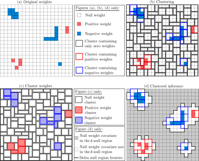
Equivalently, the sparse-smooth assumption with parameter $\delta$ holds if the distance between the two closest weights of opposite sign is larger than $\delta$. In Figure 2-(a), we give an example of a weight map verifying the sparse-smooth assumption with $\delta=2$.

3 Statistical control with spatial tolerance

Under the spatial assumption we have discussed, discoveries that are closer than $\delta$ from the true support are not considered as false discoveries: inference at a resolution finer than $\delta$ might be unrealistic. This means that $\delta$ can be interpreted as a tolerance parameter on the (spatial) support we aim at recovering. Then, we introduce a new metric closely related to the FWER that takes into account spatial tolerance and we call it $\delta$-family wise error rate ($\delta$-FWER). A similar extension of the false discovery rate (FDR) has been introduced by Cheng et al. (2020); Nguyen et al. (2019); Gimenez and Zou (2019), but, to the best of our knowledge, this has not been considered yet for the FWER. In the following, we consider a general estimator $\hat{\bm{\beta}}$ that comes with p-values, testing the nullity of the corresponding parameters, denoted by $\hat{p}=(\hat{p}_{j})_{j\in[p]}$. Also, we denote by $S(\hat{\bm{\beta}})\subset[p]$ a general estimate of the support $S(\bm{\beta}^{*})$ derived from the estimator $\hat{\bm{\beta}}$.

Definition 3.1 ($\delta$-null hypothesis).

For all $j\in[p]$, the $\delta$-null hypothesis for the $j$-th covariates, $H^{\delta}_{0}(j)$, states that all other covariates at distance less than $\delta$ have a zero weight in the true model Equation 1; the alternative hypothesis is denoted $H^{\delta}_{1}(j)$:

$$\begin{split}&H^{\delta}_{0}(j):\text{``for all}~{}k\in[p]~{}\text{such that}~{}d(j,k)\leq\delta,~{}\bm{\beta}^{*}_{k}=0\text{''}\enspace,\\ &H^{\delta}_{1}(j):\text{``there exists}~{}k\in[p]~{}\text{such that}~{}d(j,k)\leq\delta~{}\text{and }\,\bm{\beta}^{*}_{k}\neq 0\text{''}\enspace.\\ \end{split}$$

Thus, we say that a $\delta$-type 1 error is made if a null covariate $j\in[p]$ is selected, i.e., $j\in S(\hat{\bm{\beta}})$, while $H^{\delta}_{0}(j)$ holds true. Taking $\delta=0$ recovers the usual null-hypothesis $H_{0}(j):\text{``}\bm{\beta}^{*}_{j}=0$” and usual type 1 error.

Definition 3.2 (Control of the $\delta$-type 1 error).

The p-value related to the $j$-th covariate denoted by $\hat{p}_{j}$ controls the $\delta$-type 1 error if, under $H^{\delta}_{0}(j)$, for all $\alpha\in(0,1)$, we have:

$$\mathbb{P}(\hat{p}_{j}\leq\alpha)\leq\alpha\enspace,$$

where $\mathbb{P}$ is the probability distribution with respect to the random dataset of observations $(\mathbf{X},\mathbf{y})$.

Definition 3.3 ($\delta$-null region).

The set of indexes of covariates verifying the $\delta$-null hypothesis is called the $\delta$-null region and is denoted by $N^{\delta}(\bm{\beta}^{*})$ (or simply $N^{\delta}$):

$$N^{\delta}(\bm{\beta}^{*})=\left\{j\in[p]:\text{for all}~{}k\in[p],~{}d(j,k)\leq\delta~{}\text{implies that}~{}\bm{\beta}^{*}_{k}=0\right\}\enspace.$$

When $\delta=0$ the $\delta$-null region is simply the null region : $N^{0}(\bm{\beta}^{*})=N(\bm{\beta}^{*})$. We also point out the nested property of $\delta$-null regions with respect to $\delta$: for $0\leq\delta_{1}\leq\delta_{2}$ we have $N^{\delta_{2}}(\bm{\beta}^{*})\subseteq N^{\delta_{1}}(\bm{\beta}^{*})\subseteq N(\bm{\beta}^{*})$ (see Figure 2-(d) for an example of $\delta$-null region).

Definition 3.4 (Rejection region).

Given a family of p-values $\hat{p}=(\hat{p}_{j})_{j\in[p]}$ and a threshold $\alpha\in(0,1)$, the rejection region, $R_{\alpha}(\hat{p})$, is the set of indexes having a p-value lower than $\alpha$:

$$R_{\alpha}(\hat{p})=\left\{j\in[p]:\hat{p}_{j}\leq\alpha\right\}\enspace.$$

Definition 3.5 ($\delta$-type 1 error region).

Given a family of p-values $\hat{p}=(\hat{p}_{j})_{j\in[p]}$ and a threshold $\alpha\in(0,1)$, the $\delta$-type 1 error region at level $\alpha$ is $\mathscr{E}_{\alpha}^{\delta}$, the set of indexes belonging both to the $\delta$-null region and to the rejection region at level $\alpha$. We also refer to this region as the erroneous rejection region at level $\alpha$ with tolerance $\delta$:

$$\mathscr{E}^{\delta}_{\alpha}(\hat{p})=N^{\delta}\cap R_{\alpha}(\hat{p})\enspace.$$

When $\delta=0$ the $\delta$-type 1 error region recovers the type 1 error region which is denoted by $\mathscr{E}_{\alpha}(\hat{p})$. Again, one can verify a nested property: for $0\leq\delta_{1}\leq\delta_{2}$ we have $\mathscr{E}_{\alpha}^{\delta_{2}}(\hat{p})\subseteq\mathscr{E}_{\alpha}^{\delta_{1}}(\hat{p})\subseteq\mathscr{E}_{\alpha}(\hat{p})$.

Definition 3.6 ($\delta$-family wise error rate).

Given a family of p-values $\hat{p}=(\hat{p}_{j})_{j\in[p]}$ and a threshold $\alpha\in(0,1)$, the $\delta$-FWER at level $\alpha$ with respect to the family $\hat{p}$, denoted $\delta\mbox{-FWER}_{\alpha}(\hat{p})$, is the probability that the $\delta$-type 1 error region at level $\alpha$ is not empty:

$$\delta\mbox{-FWER}_{\alpha}(\hat{p})=\mathbb{P}(|\mathscr{E}^{\delta}_{\alpha}(\hat{p})|\geq 1)=\mathbb{P}(\min_{j\in N^{\delta}}\hat{p}_{j}\leq\alpha)\enspace.$$

Definition 3.7 ($\delta$-FWER control).

We say that the family of p-values $\hat{p}=(\hat{p}_{j})_{j\in[p]}$ controls the $\delta$-FWER if, for all $\alpha\in(0,1)$:

$$\delta\mbox{-FWER}_{\alpha}(\hat{p})\leq\alpha\enspace.$$

When $\delta=0$ the $\delta$-FWER is the usual FWER. Additionally, for $0\leq\delta_{1}\leq\delta_{2}$, one can verify that $\delta_{2}\mbox{-FWER}_{\alpha}(\hat{p})\leq\delta_{1}\mbox{-FWER}_{\alpha}(\hat{p})\leq\mbox{FWER}_{\alpha}(\hat{p})$. Thus, $\delta$-FWER control is a weaker property than usual FWER control.

4 $\delta$-FWER control with clustered inference algorithms

4.1 Clustered inference algorithms

A clustered inference algorithm consists in partitioning the covariates into groups (or clusters) before applying a statistical inference procedure. In Algorithm 1, we describe a standard clustered inference algorithm that produces a (corrected) p-value family on the parameters of the model Equation 1. In this algorithm, in addition to the observations ($\mathbf{X},\mathbf{y}$), we take as input the transformation matrix $\mathbf{A}\in\mathbb{R}^{p\times C}$ which maps and averages covariates into $C$ clusters. The statistical_inference function corresponds to a given statistical inference procedure that takes as inputs the clustered data $\mathbf{Z}$ and the target $\mathbf{y}$ and produces valid p-values for every cluster. If $C<n$, least squares are suitable, otherwise, procedures such as multi-sample split (Wasserman and Roeder, 2009; Meinshausen et al., 2009), corrected ridge (Bühlmann, 2013) or desparsified Lasso (Zhang and Zhang, 2014; van de Geer et al., 2014; Javanmard and Montanari, 2014) might be relevant whenever their assumptions are verified. Then, the computed p-values are corrected for multiple testing by multiplying by a factor $C$. Finally, covariate-wise p-values are inherited from the corresponding cluster-wise p-values.

input : $\mathbf{X}\in\mathbb{R}^{n\times p},\mathbf{y}\in\mathbb{R}^{n},\mathbf{A}\in\mathbb{R}^{p\times C}$

$\mathbf{Z}=\mathbf{X}\mathbf{A}$ ;

  // compressed design matrix

$\hat{p}^{\mathcal{G}}=\texttt{statistical\_inference}(\mathbf{Z},\mathbf{y})$ ;

  // uncorrected cluster-wise p-values

$\hat{q}^{\mathcal{G}}=C\times\hat{p}^{\mathcal{G}}$ ;

  // corrected cluster-wise p-values

for $j=1,\dots,p$ do

       $\hat{q}_{j}=\hat{q}^{\mathcal{G}}_{c}$ if $j$ in cluster $c$ ;

        // corrected covariate-wise p-values

      

return $\hat{q}=(\hat{q}_{j})_{j\in[p]}$ ;

  // family of corrected covariate-wise p-values

Algorithm 1 Clustered inference

input : $\mathbf{X}\in\mathbb{R}^{n\times p},\mathbf{y}\in\mathbb{R}^{n}$

param : $C,B$

for $b=1,\dots,B$ do

       $\mathbf{X}^{(b)}=\texttt{sampling}(\mathbf{X})$ ;

        // sampling rows of $\mathbf{X}$

       $\mathbf{A}^{(b)}=\texttt{clustering}(q,\mathbf{X}^{(b)})$ ;

        // transformation matrix

       $\hat{q}^{(b)}=\texttt{clustered\_inference}(\mathbf{X},\mathbf{y},\mathbf{A}^{(b)})$ ;

        // families of corr. covariate-wise p-val.

      

for $j=1,\dots,p$ do

       $\hat{q}_{j}=\texttt{ensembling}(\{\hat{q}_{j}^{(b)},b\in[B]\})$ ;

        // aggregated corrected covariate-wise p-values

      

return $\hat{q}=(\hat{q}_{j})_{j\in[p]}$ ;

  // family of aggregated corrected covariate-wise p-values

Algorithm 2 Ensembled clustered inference

Ensembled clustered inference algorithms correspond to the ensembling of several clustered inference solutions for different choice of clusterings using the p-value aggregation proposed by Meinshausen et al. (2009). In Algorithm 2, we give a standard ensembled clustered inference algorithm that produces a (corrected) p-value family on the parameters of the model Equation 1. In this algorithm, the sampling function corresponds to a subsampling of the data, i.e., a subsampling of the rows of $\mathbf{X}$. The clustering function derives a choice of clustering in $C$ clusters, it produces a transformation matrix $\mathbf{A}^{(b)}\in\mathbb{R}^{p\times C}$ that should vary for each bootstrap $b\in[B]$ since the subsampled data $\mathbf{X}^{(b)}$ varies. Once the clustering inference steps are completed, the ensembling function aggregates the $B$ (corrected) p-value families into a single one.

Figure 1 can help the reader to better understand the organization of the next sections, aiming eventually at establishing the $\delta$-FWER control property of the clustered inference and ensembled clustered inference algorithms.

Figure 1: Organization of Section 4.

4.2 Compressed representation

The motivation for using groups of covariates that are spatially concentrated is to reduce the dimension while preserving large-scale data structure. The number of groups is denoted by $C<p$ and, for $r\in[q]$, we denote by $G_{r}$ the $r$-th group. The collection of all the groups is denoted by $\mathcal{G}=\{G_{1},G_{2},\ldots,G_{C}\}$ and forms a partition of $[p]$. Every group representative variable is defined by the average of the covariates it contains. Then, denoting by $\mathbf{Z}\in\mathbb{R}^{n\times C}$ the compressed random design matrix that contains the group representative variables in columns and, without loss of generality, assuming a suitable ordering of the columns of $\mathbf{X}$, dimension reduction can be written:

$$\mathbf{Z}=\mathbf{X}\mathbf{A}\enspace,$$ (2)

where $\mathbf{A}\in\mathbb{R}^{p\times q}$ is the transformation matrix defined by:

$$\mathbf{A}=\left[\begin{matrix}\alpha_{1}\rule[2.58334pt]{10.76385pt}{0.5pt}\alpha_{1}&0\rule[2.58334pt]{10.76385pt}{0.5pt}0&\ldots&0\rule[2.58334pt]{10.76385pt}{0.5pt}0\\ 0\rule[2.58334pt]{10.76385pt}{0.5pt}0&\alpha_{2}\rule[2.58334pt]{10.76385pt}{0.5pt}\alpha_{2}&\ldots&0\rule[2.58334pt]{10.76385pt}{0.5pt}0\\ \vdots&\vdots&\ddots&\vdots\\ 0\rule[2.58334pt]{10.76385pt}{0.5pt}0&0\rule[2.58334pt]{10.76385pt}{0.5pt}0&\ldots&\alpha_{C}\rule[2.58334pt]{10.76385pt}{0.5pt}\alpha_{C}\\ \end{matrix}\right]\enspace,$$

where $\alpha_{c}={1}/{|G_{c}|}$ for all $c\in[C]$. Consequently, the distribution of the $i$-th row of $\mathbf{Z}$ is given by $\mathbf{Z}_{i,.}\sim\mathcal{N}_{q}(0,\bm{\Upsilon})$, where $\bm{\Upsilon}=\mathbf{A}^{\top}\bm{\Sigma}\mathbf{A}$. The correlation between the groups $r\in[q]$ and $l\in[q]$ is given by $\operatorname{Cor}(\mathbf{Z}_{.,r},\mathbf{Z}_{.,l})=\bm{\Upsilon}_{r,l}/\sqrt{\bm{\Upsilon}_{r,r}\bm{\Upsilon}_{l,l}}$. As mentioned in Bühlmann et al. (2013), because of the Gaussian assumption in Equation 1, we have the following compressed representation:

$$\mathbf{y}=\mathbf{Z}\bm{\theta}^{*}+\bm{\eta}\enspace,$$ (3)

where $\bm{\theta}^{*}\in\mathbb{R}^{q}$, $\bm{\eta}\sim\mathcal{N}(0,\sigma_{\eta}^{2}\mathbf{I}_{n})$, $\sigma_{\eta}\geq\sigma_{\varepsilon}>0$ and $\bm{\eta}$ is independent of $\mathbf{Z}$.

Remark 4.1.

Dimension reduction is not the unique desirable effect of clustering with regards to statistical inference. Indeed, this clustering-based design compression also generally improves the conditioning of the problem. Assumptions needed for valid statistical inference are thus more likely to be met. For more details about this conditioning enhancement, the reader may refer to Bühlmann et al. (2013).

4.3 Properties of the compressed model weights

Figure 2: Clustered inference mechanism on 2D-spatially structured data. Item a: Example of weight map with a 2D-structure. Voxels represent covariates, with blue (resp. red) corresponding to negative (resp. positive) weights; others are null weights. Item b: Arbitrary choice of spatially constrained clustering with a diameter of $\delta=2$ units for the $\ell_{1}$-distance. Rectangles delimited by black lines represent clusters that contain only zero-weight covariates. Blue (resp. red) rectangles refer to clusters that contain negative-weight (resp. positive) covariates. Item c: Compressed model weights: under the assumptions of Proposition 4.1, the cluster weights share the same signs as the covariate weights they contain. Blue (resp. red) rectangles correspond to negative-weight (resp. positive-weights) clusters. Item d: The grey area corresponds to the $\delta$-null region ($\delta=2$). Under the same assumptions, the non-zero weight groups have no intersection with the $\delta$-null region.

We now give a property of the weights of the compressed problem which is a consequence of Bühlmann et al. (2013, Proposition 4.3).

Proposition 4.1.

Considering the Gaussian linear model in Equation 1 and assuming:

$$\begin{split}&(i)~{}\text{for all}~{}c\in[C],~{}\text{for all}~{}(j,k)\in(G_{c})^{2},~{}\bm{\Sigma}_{j,k}\geq 0\enspace,\\ &(ii)~{}\text{for all}~{}c\in[C],~{}\text{for all}~{}c^{\prime}\in[C]\setminus\{c\},~{}\bm{\Upsilon}_{c,c^{\prime}}=0\enspace,\\ &(iii)~{}\text{for all}~{}c\in[C],\left(\bm{\beta}^{*}_{j}\geq 0~{}\text{for all}~{}j\in G_{c}\right)\operatorname{or}\left(\bm{\beta}^{*}_{j}\leq 0~{}\text{for all}~{}j\in G_{c}\right)\enspace,\\ \end{split}$$

then, in the compressed representation Equation 3, for $c\in[C]$, $\bm{\theta}_{c}^{*}\neq 0$ if and only if there exists $j\in G_{c}$ such that $\bm{\beta}_{j}^{*}\neq 0$. If such an index $j$ exists then $\operatorname{sign}(\bm{\theta}_{r}^{*})=\operatorname{sign}(\bm{\beta}_{j}^{*})$.

Proof.

See Section E.1. ∎

Assumption $(i)$ states that the covariates in a group are all positively correlated. Let us define the group diameter (or cluster diameter) of $G_{c}$ by the distance that separates its two most distant covariates, i.e., $\operatorname{Diam}(G_{c})=\max\{d(j,k):(j,k)\in(G_{c})^{2}\}$ and the clustering diameter of $\mathcal{G}$ by the largest group diameter, i.e., $\operatorname{Diam}(\mathcal{G})=\max\{\operatorname{Diam}(G_{c}):c\in[C]\}$. In Figure 2-(b), we propose a clustering of the initial weight map in Figure 2-(a) for which the clustering diameter is equal to $2$ for the $\ell_{1}$ distance. Assumption $(i)$ notably holds when $\operatorname{Diam}(\mathcal{G})\leq\delta$ under the spatial homogeneity assumption (Assumption 2.1) with parameter $\delta$. Assumption $(ii)$ assumes independence of the groups. A sufficient condition is when the covariates covariance matrix $\bm{\Sigma}$ is block diagonal, with blocks coinciding with the group structure; i.e., assumption $(ii)$ holds when covariates of different groups are independent. In practice, this assumption may be unmet, and we relax it in Appendix B. Assumption $(iii)$ states that all the weights in a group share the same sign. This is notably the case when the clustering diameter is smaller than $\delta$ and the weight map satisfies the sparse-smooth assumption (Assumption 2.2) with parameter $\delta$. For instance, a clustering-based compressed representation of the weight map in Figure 2-(a) is given in Figure 2-(c).

4.4 Statistical inference on the compressed model

To perform the statistical inference on the compressed problem Equation 3, we could consider any statistical inference procedure that produces cluster-wise p-values $\hat{p}^{\mathcal{G}}=(\hat{p}^{\mathcal{G}}_{c})_{c\in[C]}$, given a choice of clustering $\mathcal{G}$, that control the type 1 error. More precisely, for any $c\in[C]$, under $H_{0}(G_{c})$, i.e., the null hypothesis which states that $\theta_{c}^{*}$ is equal to zero in the compressed model, we assume that the p-value associated with the $c$-th cluster verifies:

$$\begin{split}\mathbb{P}(\hat{p}^{\mathcal{G}}_{c}\leq\alpha)\leq\alpha\enspace.\end{split}$$ (4)

To correct for multiple comparisons, we consider Bonferroni correction (Dunn, 1961) which is a conservative procedure but has the advantage of being valid without any additional assumptions. Furthermore, here the correction factor is only equal to the number of groups, not the number of covariates. Then, the family of corrected cluster-wise p-values $\hat{q}^{\mathcal{G}}=(\hat{q}^{\mathcal{G}}_{c})_{c\in[C]}$ is defined by:

$$\hat{q}^{\mathcal{G}}_{c}=\min\{1,C\times{\hat{p}^{\mathcal{G}}_{c}}\}\enspace.$$ (5)

Let us denote by $N_{\mathcal{G}}(\bm{\theta}^{*})$ (or simply $N_{\mathcal{G}}$) the null region in the compressed problem for a given choice of clustering $\mathcal{G}$, i.e., $N_{\mathcal{G}}(\bm{\theta}^{*})=\left\{c\in[C]:\bm{\theta}^{*}_{c}=0\right\}$. Then, for all $\alpha\in(0,1)$:

$$\mbox{FWER}_{\alpha}(\hat{q}^{\mathcal{G}})=\mathbb{P}(\min_{c\in N_{\mathcal{G}}}\hat{q}^{\mathcal{G}}_{c}\leq\alpha)\leq\alpha\enspace.$$ (6)

This means that the cluster-wise p-value family $\hat{q}^{\mathcal{G}}$ controls FWER.

4.5 De-grouping

Given the families of cluster-wise p-values $\hat{p}^{\mathcal{G}}$ and corrected p-values $\hat{q}^{\mathcal{G}}$ as defined in Equation 10 and Equation 5, our next aim is to derive families of p-values and corrected p-values related to the covariates of the original problem. To construct these families, we simply set the (corrected) p-value of the $j$-th covariate to be equal to the (corrected) p-value of its corresponding group:

$$\begin{split}&\text{for all}~{}j\in[p],\quad\hat{p}_{j}=\sum_{c\in[C]}\mathds{1}_{\{j\in G_{c}\}}~{}\hat{p}^{\mathcal{G}}_{c}\enspace,\\ &\text{for all}~{}j\in[p],\quad\hat{q}_{j}=\sum_{c\in[C]}\mathds{1}_{\{j\in G_{c}\}}~{}\hat{q}^{\mathcal{G}}_{c}\enspace.\\ \end{split}$$ (7)

Proposition 4.2.

Under the assumptions of Proposition 4.1 and assuming that the clustering diameter is smaller than $\delta$, then:

(i) elements of the family $\hat{p}$ defined in Equation 7 control the $\delta$-type 1 error:

$$\text{for all}~{}j\in N^{\delta},~{}\text{for all}~{}\alpha\in(0,1),~{}\mathbb{P}(\hat{p}_{j}\leq\alpha)\leq\alpha\enspace,$$

(ii) the family $\hat{q}$ defined in Equation 7 controls the $\delta$-FWER:

$$\text{for all}~{}\alpha\in(0,1),~{}\mathbb{P}(\min_{j\in N^{\delta}}(\hat{q}_{j})\leq\alpha)\leq\alpha\enspace.$$

Proof.

See Section E.2. ∎

The previous de-grouping properties can be seen in Figure 2-(d). Roughly, since all the clusters that intersect the $\delta$-null region have low p-value with low probability, one can conclude that all the covariates of the $\delta$-null region also have low p-value with low probability.

4.6 Ensembling

Let us consider $B$ families of corrected p-values that control the $\delta$-FWER. For any $b\in[B]$, we denote by $\hat{q}^{(b)}$ the $b$-th family of corrected p-values. Then, we show that the ensembling method proposed in Meinshausen et al. (2009) yields a family that also enforces $\delta$-FWER control.

Proposition 4.3.

Assume that, for $b\in[B]$, the p-value families $\hat{q}^{(b)}$ control the $\delta$-FWER. Then, for any $\gamma\in(0,1)$, the ensembled p-value family $\tilde{q}(\gamma)$ defined by:

$$\text{for all}~{}j\in[p],~{}\tilde{q}_{j}(\gamma)=\min\left\{1,\gamma\mbox{-quantile}\left(\left\{\frac{\hat{q}^{(b)}_{j}}{\gamma}:b\in[B]\right\}\right)\right\}\enspace,$$ (8)

controls the $\delta$-FWER.

Proof.

See Section E.3. ∎

4.7 $\delta$-FWER control

We can now state our main result: the clustered inference and ensembled clustered inference algorithms control the $\delta$-FWER.

Theorem 4.1.

Assume the model given in Equation 1 and that the data structure assumptions, Assumption 2.1 and Assumption 2.2, are satisfied for a distance parameter larger than $\delta$. Assume that all the clusterings considered have a diameter smaller than $\delta$. Assume that the uncorrelated cluster assumption, i.e., assumption $(ii)$ of Proposition 4.1, is verified for each clustering and further assume that the statistical inference performed on the compressed model Equation 3 is valid, i.e., Equation 4 holds. Then, the p-value family obtained from the clustered inference algorithm controls the $\delta$-FWER. Additionally, the p-value family derived by the ensembled clustered inference algorithm controls the $\delta$-FWER.

Proof.

See Section E.4. ∎

Remark 4.2.

When the type 1 error control offered by the statistical inference procedure is only asymptotic, the result stated by Theorem 4.1 remains true asymptotically. This is notably the case when using desparsified Lasso: under the assumptions of Theorem 4.1 and the assumptions specific to desparsified Lasso (cf. Appendix A), ensemble of clustered desparsified Lasso (EnCluDL) controls the $\delta$-FWER asymptotically.

5 Numerical Simulations

5.1 CluDL and EnCluDL

For testing the (ensembled) clustered inference algorithms, we have decided to make the inference step using the desparsified Lasso (Zhang and Zhang, 2014; van de Geer et al., 2014; Javanmard and Montanari, 2014) leading to the clustered desparsified Lasso (CluDL) and the ensemble of clustered desparsified Lasso (EnCluDL) algorithms that were first presented in Chevalier et al. (2018).

In Appendix A, we detail the assumptions and refinements that occur when choosing the desparsified Lasso to perform the statistical inference step. A notable difference is the fact that all the results becomes asymptotic. In Appendix C, we present a diagram illustrating the mechanism of EnCluDL and analyse its numerical complexity.

5.2 2D Simulation

We run a series of simulations on 2D data in order to give empirical evidence of the theoretical properties of CluDL and EnCluDL and compare their recovery properties with two other procedures. For an easier visualization of the results, we consider one central scenario, whose parameters are written in bold in the following of this section, with several variations, changing only one parameter at a time.

In all these simulations, the feature space considered is a $2$D square with edge length $H=40$ leading to $p=H^{2}=\numprint{1600}$ covariates, with a sample size $n\in\{50,\mathbf{100},200,400\}$. To construct $\bm{\beta}^{*}$, we define a $2$D weight map $\tilde{\bm{\beta}}^{*}$ with four active regions (as illustrated in Figure 3) and then flatten $\tilde{\bm{\beta}}^{*}$ to a vector ${\bm{\beta}}^{*}$ of size $p$. Each active region is a square of width $h\in\{2,\mathbf{4},6,8\}$, leading to a size of support of $1\%$, $\mathbf{4\%}$, $9\%$ or $16\%$. To construct the design matrix, we first build a $2$D data matrix $\tilde{\mathbf{X}}$ by drawing $p$ random normal vectors of size $n$ that are spatially smoothed with a $2$D Gaussian filter to create a correlation structure related to the covariates’ spatial organization. The same flattening process as before is used to get the design matrix $\mathbf{X}\in\mathbb{R}^{n\times p}$. The intensity of the spatial smoothing is adjusted to achieve a correlation between two adjacent covariates (local correlation) of $\rho\in\{0.5,\mathbf{0.75},0.9,0.95\}$. We also set the noise standard deviation $\sigma_{\varepsilon}\in\{1,\mathbf{2},3,4\}$, which corresponds to a signal to noise ratio (SNR) $\mbox{SNR}_{y}\in\{6.5,\mathbf{3.5},2.2,1.5\}$, where the SNR is defined by $\operatorname{SNR}_{y}=\lVert{\mathbf{X}\bm{\beta}^{*}}\rVert_{2}/\lVert{\bm{\varepsilon}}\rVert_{2}$. For each scenario, we run $100$ simulations to derive meaningful statistics. A Python implementation of the simulations and procedures presented in this paper is available on https://github.com/ja-che/hidimstat. Regarding the clustering step in CluDL and EnCluDL, we used a spatially constrained agglomerative clustering algorithm with Ward criterion. This algorithm is popular in many applications (Varoquaux et al., 2012; Dehman et al., 2015), as it tends to create compact, balanced clusters. Since the optimal number of clusters $C$ is unknown a priori, we have tested several values $C\in[100;400]$. A smaller $C$ generally improves recovery, but entails a higher spatial tolerance. Following theoretical considerations, we compute the largest cluster diameter for every value of $C$ and set $\delta$ to this value. We obtained the couples $(C,\delta)\in\{(100,8),(200,6),(300,5),(400,4)\}$. The tolerance region is represented in Figure 3 for $\delta=6$. Concerning EnCluDL, we took a number of bootstraps $B$ equal to $25$ as we observed that it was sufficient to benefit from most of the effect of clustering randomization.

5.3 Alternative methods

We compare the recovering properties of CluDL and EnCluDL with two other procedures: desparsified Lasso and knockoffs. Contrarily to CluDL and EnCluDL, none of these includes a compression step. The version of the desparsified Lasso we have tested is the one presented in van de Geer et al. (2014), that outputs p-values. Using Bonferroni correction it controls the classical FWER at any desired rate. The original version of knockoffs (Barber and Candès, 2015; Candès et al., 2018) only controls the false discovery rate (FDR) which is a weaker control than the classical FWER. Yet Janson and Su (2016) modifies the covariate selection process leading to a procedure that controls the $k$-FWER, i.e., the probability of making at least $k$ false discoveries. We tested this last extension of knockoffs. Depending on the nominal rate at which we want to control the $k$-FWER, the choice of $k$ is not arbitrary. More precisely, if we want a $k$-FWER control at $10\%$, we need to tolerate $k=4$ at least, otherwise the estimated support would always be empty.

Since $k$-FWER and $\delta$-FWER controls are both weaker than the usual FWER control whenever $k>1$ and $\delta>0$, one can expect desparsified Lasso to be less powerful than knockoffs, CluDL and EnCluDL. Besides, there is no relation between $k$-FWER and $\delta$-FWER controls when $k>1$ and $\delta>0$, hence it is not possible to establish which one is less prohibitive for support recovery. However, when data are spatially structured, $\delta$-FWER control might be more relevant since it controls the very undesirable far-from-support false discoveries.

5.4 Results

Figure 3: True support and estimated support for the first seed of the central scenario. Left: The support in yellow is composed of four regions of width $h=4$ covariates. The tolerance region in green surrounds the support, its width is $\delta=6$ covariates. The remaining covariates in blue form the $\delta$-null region. Others: The yellow squares are the covariates selected by each method. Knockoffs selects few covariates when controlling the $k$-FWER at $10\%$ for $k=4$. Desparsified Lasso only retrieves $3$ covariates when controlling the FWER at $10\%$. For $C=200$, CluDL and EnCluDL have good power and control the $\delta$-FWER at $10\%$ for $\delta=6$.

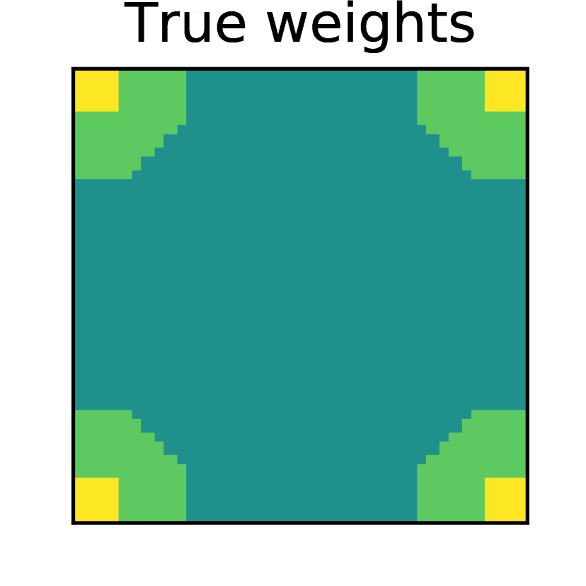
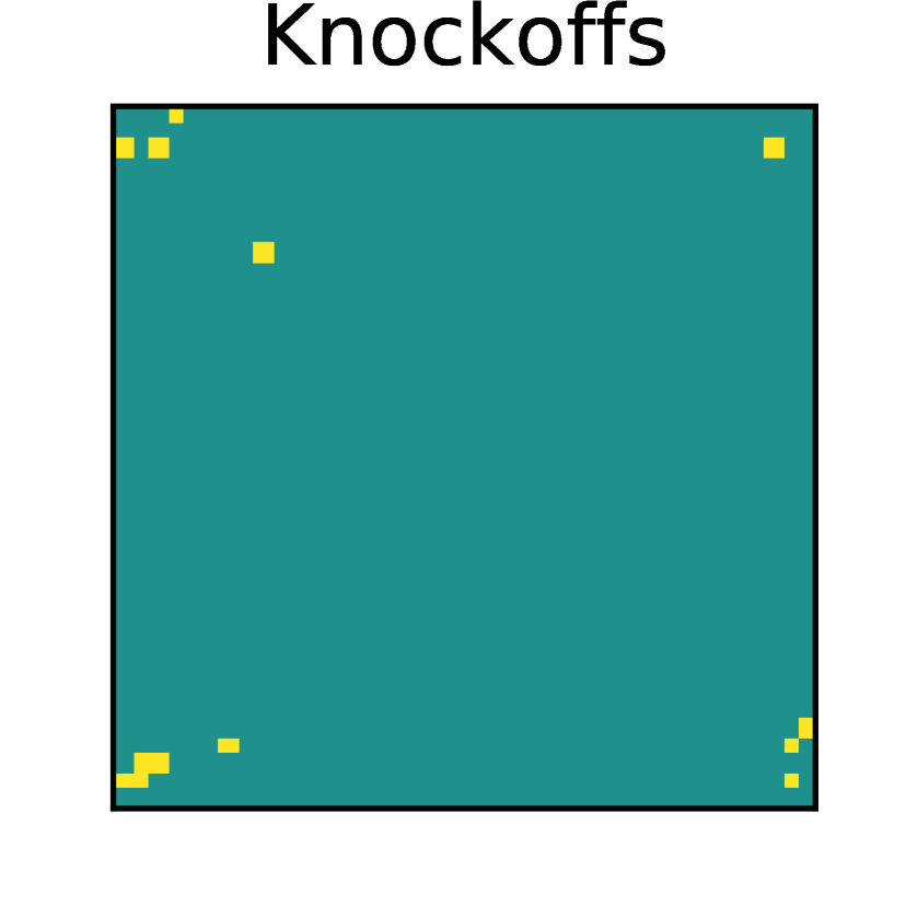
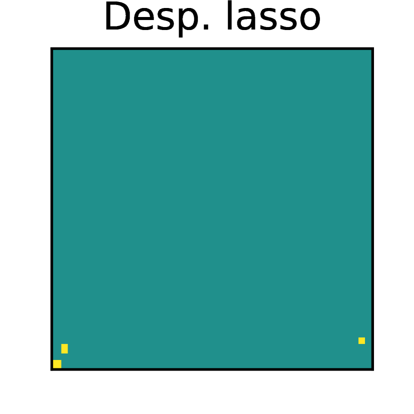
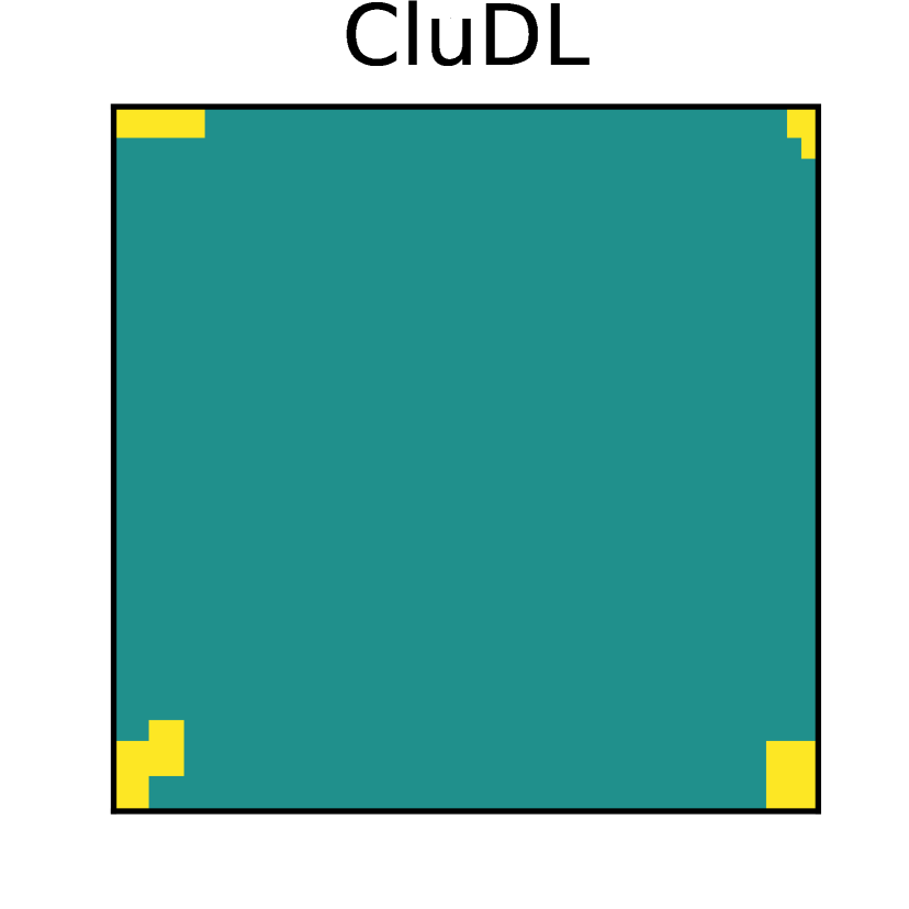
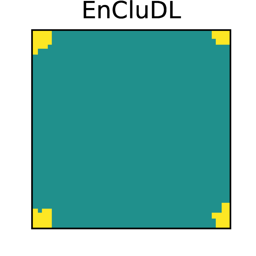
In Figure 3, we plot the maps estimated by knockoffs, desparsified Lasso, CluDL and EnCluDL for $C=200$ when solving the first seed of the central scenario simulation. Regarding knockoffs and desparsified Lasso solutions, we notice that the power is low and the methods select few covariates in each predictive region. The CluDL method is more powerful and recovers groups of covariates that correspond more closely to the true weights. However, the shape of the CluDL solution depends on the clustering choice. The EnCluDL solution seems even more powerful than the CluDL one and recovers groups of covariates that correspond almost perfectly to the true weights. Both CluDL and EnCluDL are only accurate up to the spatial tolerance which is $\delta=6$, but EnCluDL fits the ground truth more tightly.

Figure 4: Results for fixed simulation parameters corresponding to the central scenario simulation. The green line with circles correspond to knockoffs, the brown line with triangles is the desparsified Lasso, the purple squared line correspond to CluDL and the blue plain line is EnCluDL. Left: Empirical FWER for desparsified Lasso, $k$-FWER for knockoffs and $\delta$-FWER for CluDL and EnCluDL. The $80\%$ confidence intervals are obtained by Binomial approximation. Right: Median true positive rate (TPR) for all the procedures, together with $80\%$ confidence interval obtained by taking the first decile and last decile TPR.

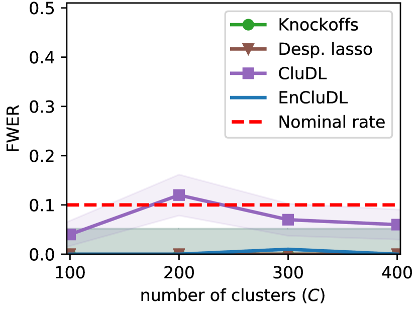
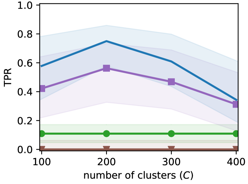
In Figure 4, we focus on the central scenario to get more insight about the statistical properties of the methods and the influence of the $C$ hyper-parameter for CluDL and EnCluDL. First, we observe that all methods reach the targeted control: desparsified Lasso controls the FWER, knockoffs control the $k$-FWER and, CluDL and EnCluDL control the $\delta$-FWER. Second, considering the true positive rates (TPR), we notice that the methods that do not integrate a compression step, i.e., knockoffs and desparsified Lasso, have a limited statistical power due to $n\ll p$. However, CluDL has decent power and EnCluDL improves over CluDL thanks to clustering randomization. Finally, CluDL and EnCluDL are flexible with respect to the choice of $C$ since the TPR varies quite slowly with $C$.

We have also studied the influence of the simulation parameters by varying one parameter of the central scenario. The corresponding results are available in Appendix D. The main conclusion gained from these complementary results is the fact that, up to the limit given by the desired spatial tolerance $\delta$, the choice of $C$ should be made in function of the data structure. More precisely, good clustering creates clusters that are weakly correlated and contains covariates that are highly correlated. This observation is linked to assumption ($ii$) of Proposition 4.1.

6 Discussion

When $n\ll p$, statistical inference on predictive model parameters is a hard problem. However, when the data are spatially structured, we have shown that ensembled clustered inference procedures are attractive, as they exhibit statistical guarantees and good power. The price to pay is to accept that inference is only accurate up to spatial distance $\delta$ corresponding to the clustering diameter, thus replacing FWER with $\delta$-FWER control guarantees.

One of the most obvious field of application of this class of algorithms is neuroscience where it can be used to solve source localization problems. In that regards, a wide empirical validation of EnCluDL has been conducted in Chevalier et al. (2021) including fMRI data experiments. Also, an extension of EnCluDL was proposed in Chevalier et al. (2020) to address the magneto/electroencephalography source localization problem which involves spatio-temporal data.

With EnCluDL, the statistical inference step is performed by the desparsified Lasso. In Nguyen et al. (2019), another ensembled clustered inference method that leverages the knockoff technique (Barber and Candès, 2015) leading to a procedure called ECKO has been tested. However, formal $\delta$-FDR control guarantees have not been established yet for this model. It would be also quite natural to try other inference techniques such as the (distilled) conditional randomization test (Candès et al., 2018; Liu and Janson, 2020).

In the present work, we have only considered the linear regression setup. However, combining the same algorithmic scheme with statistical inference solutions for generalized linear models, we could extend this work to the logistic regression setup. This would extend the usability of ensembled clustered inference to many more application settings.

Supplementary material

Supplementary material available online includes an analysis of the technical assumptions and refinements that occur when choosing the desparsified Lasso to perform the statistical inference step in Appendix A, a diagram summarizing EnCluDL and a study of the complexity of EnCluDL in Appendix C, a proposition for relaxing assumption $(ii)$ of Proposition 4.1 in Appendix B, complementary results for studying the influence of the simulation parameters in Appendix D and the proofs in Appendix E.

Supplementary material for “Spatially relaxed inference on high-dimensional linear models"

Appendix A Desparsified Lasso on the compressed model

Here, we clarify the assumptions and refinements that occur when chosing the desparsified Lasso as the procedure that performs the statistical inference on the compressed model. The desparsified Lasso was first developed in Zhang and Zhang [2014] and Javanmard and Montanari [2014], and thoroughly analyzed in van de Geer et al. [2014]. Following notation in Eq. Equation 3, the true support in the compressed model is denoted by $S(\bm{\theta}^{*})=\{c\in[C]:\bm{\theta}^{*}_{c}\neq 0\}$ and its cardinality by $s(\bm{\theta}^{*})=|S(\bm{\theta}^{*})|$. We also denote by $\bm{\Omega}\in\mathbb{R}^{C\times C}$ the inverse of the population covariance matrix of the groups, i.e., $\bm{\Omega}=\bm{\Upsilon}^{-1}$. Then, for $c\in[C]$, the sparsity of the $c$-th row of $\bm{\Omega}$ (or $c$-th column) is $s(\bm{\Omega}_{c,.})=|S(\bm{\Omega}_{c,.})|$, where $S(\bm{\Omega}_{c,.})=\{c^{\prime}\in[C]:\bm{\Omega}_{c,c^{\prime}}\neq 0\}$. We also denote the smallest eigenvalue of $\bm{\Upsilon}$ by $\phi_{\min}(\bm{\Upsilon})>0$. We can now state the assumptions required for probabilistic inference with desparsified Lasso [van de Geer et al., 2014]:

Theorem A.1 (Theorem 2.2 of van de Geer et al. [2014]).

Considering the model in Eq. Equation 3 and assuming:

$$\begin{split}&(i)~{}1/\phi_{\min}(\bm{\Upsilon})=\mathcal{O}(1)\enspace,\\ &(ii)~{}\max_{c\in[C]}(\bm{\Upsilon}_{c,c})=\mathcal{O}(1)\enspace,\\ &(iii)~{}s(\theta^{*})=o(\sqrt{n}/\log(C))\enspace,\\ &(iv)~{}\max_{c\in[C]}(s(\bm{\Omega}_{c,.}))=o(n/\log(C))\enspace,\\ \end{split}$$

then, denoting by $\hat{\bm{\theta}}$ the desparsified Lasso estimator derived from the inference procedure described in van de Geer et al. [2014], the following holds:

$$\begin{split}&\sqrt{n}(\hat{\bm{\theta}}-\bm{\theta}^{*})=\bm{\xi}+\bm{\zeta}\enspace,\\ &\bm{\xi}|\mathbf{Z}\sim\mathcal{N}(0_{C},\sigma_{\bm{\eta}}^{2}\hat{\bm{\Omega}})\enspace,\\ &\left\lVert{\bm{\zeta}}\right\rVert_{\infty}=o_{\mathbb{P}}(1)\enspace,\\ \end{split}$$

where $\hat{\bm{\Omega}}$ is such that $\left\lVert{\hat{\bm{\Omega}}-\bm{\Omega}}\right\rVert_{\infty}=o_{\mathbb{P}}(1)$.

Remark A.1.

In Theorem A.1, to compute confidence intervals, the noise standard deviation $\sigma_{\eta}$ in the compressed problem has to be estimated. We refer the reader to the surveys that are dedicated to this subject such as Reid et al. [2016], Ndiaye et al. [2017], Yu and Bien [2019].

As argued in van de Geer et al. [2014], from Theorem A.1 we obtain asymptotic confidence intervals for the $r$-th element of $\bm{\theta}^{*}$ from the following equations, for all $z_{1}\in\mathbb{R}$ and $z_{2}\in\mathbb{R}^{+}$:

$$\begin{split}&\mathbb{P}\left[\frac{\sqrt{n}(\hat{\bm{\theta}}_{c}-\bm{\theta}_{c}^{*})}{\sigma_{\eta}\sqrt{\hat{\bm{\Omega}}_{c,c}}}\leq z_{1}~{}\bigg{|}~{}\mathbf{Z}\right]-\Phi(z_{1})=o_{\mathbb{P}}(1)\enspace,\\ &\mathbb{P}\left[\frac{\sqrt{n}|\hat{\bm{\theta}}_{c}-\bm{\theta}_{c}^{*}|}{\sigma_{\eta}\sqrt{\hat{\bm{\Omega}}_{c,c}}}\leq z_{2}~{}\bigg{|}~{}\mathbf{Z}\right]-(2\Phi(z_{2})-1)=o_{\mathbb{P}}(1)\enspace,\\ \end{split}$$ (9)

where $\Phi(\cdot)$ is the cumulative distribution function of the standard normal distribution. Thus, for each $c\in[C]$ one can provide a p-value that assesses whether or not $\bm{\theta}^{*}_{c}$ is equal to zero. In the case of a two-sided single test, for each $c\in[C]$, the p-value denoted by $\hat{p}^{\mathcal{G}}_{c}$ is:

$$\hat{p}^{\mathcal{G}}_{c}=2\left(1-\Phi\left(\frac{\sqrt{n}|\hat{\bm{\theta}}_{c}|}{\sigma_{\eta}\sqrt{\hat{\bm{\Omega}}_{c,c}}}\right)\right)\enspace.$$ (10)

Under $H_{0}(G_{c})$, from Equation 9, we have, for any $\alpha\in(0,1)$:

$$\begin{split}\mathbb{P}(\hat{p}^{\mathcal{G}}_{c}\leq\alpha~{}|~{}\mathbf{Z})&=1-\mathbb{P}\left[\frac{\sqrt{n}|\hat{\bm{\theta}}_{c}|}{\sigma_{\eta}\sqrt{\hat{\bm{\Omega}}_{c,c}}}\leq\Phi^{-1}\left(1-\frac{\alpha}{2}\right)~{}\bigg{|}~{}\mathbf{Z}\right]\\ &=\alpha+o_{\mathbb{P}}(1)\enspace.\end{split}$$ (11)

Then, Equation 11 shows that the p-values $\hat{p}^{\mathcal{G}}_{c}$ asymptotically control type 1 errors. Using the Bonferroni correction, the family of corrected p-values $\hat{q}^{\mathcal{G}}=(\hat{q}^{\mathcal{G}}_{c})_{c\in[C]}$ remains defined by:

$$\hat{q}^{\mathcal{G}}_{c}=\min\{1,C\times{\hat{p}^{\mathcal{G}}_{c}}\}\enspace.$$ (12)

Then, for all $\alpha\in(0,1)$:

$$\mbox{FWER}_{\alpha}(\hat{q}^{\mathcal{G}})=\mathbb{P}(\min_{c\in N_{\mathcal{G}}}\hat{q}^{\mathcal{G}}_{c}\leq\alpha~{}|~{}\mathbf{Z})\leq\alpha+o_{\mathbb{P}}(1)\enspace.$$ (13)

Then, Equation 13 shows that the p-value family $\hat{q}^{\mathcal{G}}$ asymptotically control FWER. Finally, we have shown that desparsified Lasso applied to a compressed version of the original problem provides cluster-wise p-value families $\hat{p}^{\mathcal{G}}$ and $\hat{q}^{\mathcal{G}}$ that control respectively the type 1 error and the FWER in the compressed model only asymptotically.

Appendix B Relaxing the uncorrelated clusters assumption

As noted in Section 4.3, assumption $(ii)$ of Proposition 4.1 is often unmet in practice. Here, taking the particular case in which the inference step is performed by desparsified Lasso, we relax the assumption and show that it is still possible to compute an adjusted corrected p-value that asymptotically controls the $\delta$-FWER. Hopefully, the technique used to derive this relaxation would also applicable to other parametric statistical inference methods such as corrected ridge. To better understand the development made in this section, the adjusted p-values of this section should be compared with the original p-values of Appendix A. Note that, this extension is easy to integrate in the proof of the main results Theorem 4.1 as it just requires to use the adjusted corrected p-value instead of the original corrected p-value. Also, it does not provide much more insight about clustered inference algorithms. This is why we have decided to keep this extension for Supplementary Materials.

First, we replace Proposition 4.1 by the next proposition that is a consequence of Bühlmann et al. [2013, Proposition 4.4].

Proposition B.1.

Considering the Gaussian linear model in Equation 1 and assuming:

1. for all $c\in[C]$, for all $j,k\in G^{2}_{c},~{}\operatorname{Cov}(\mathbf{X}_{.,j},\mathbf{X}_{.,k}~{}|~{}\{\mathbf{Z}_{.,c^{\prime}}:c^{\prime}\neq c\})\geq 0$  ,

2. for all  $c\in[C],~{}\text{there exists}~{}\bm{\nu}_{c}\in\mathbb{R}^{+}\text{ s.t. }~{}\text{for all}~{}j\in G_{c},~{}\text{for all}~{}k\notin G_{c}$ ,

   $$|\operatorname{Cov}(\mathbf{X}_{.,j},\mathbf{X}_{.,k}~{}|~{}\{\mathbf{Z}_{.,c^{\prime}}:c^{\prime}\neq c\})|\leq\bm{\nu}_{c}\enspace,$$

3. for all  $c\in[C],~{}\text{there exists}~{}\bm{\tau}_{c}>0\text{ s.t. }\operatorname{Var}(\mathbf{Z}_{.,c}~{}|~{}\{\mathbf{Z}_{.,c^{\prime}}:c^{\prime}\neq c\})\geq\bm{\tau}_{c}$  ,

4. for all  $c\in[C],~{}\left(\text{for all}~{}j\in G_{c},\bm{\beta}^{*}_{j}\geq 0\right)\operatorname{or}\left(\text{for all}~{}j\in G_{c},\bm{\beta}^{*}_{j}\leq 0\right)$  ,

then, in the compressed representation Equation 3, $\bm{\theta}^{*}$ admits the following decomposition:

$$\bm{\theta}^{*}=\tilde{\bm{\theta}}+\bm{\kappa}\enspace,$$ (14)

where, for all $c\in[C]$, $|\bm{\kappa}_{c}|\leq(\bm{\nu}_{c}~{}/ \bm{\tau}_{c})\lVert{\bm{\beta}^{*}}\rVert_{1}$ and $\tilde{\bm{\theta}}_{c}\neq 0$ if and only if there exists $j\in G_{c}$ such that $\bm{\beta}_{j}^{*}\neq 0$. If such an index $j$ exists then $\operatorname{sign}(\tilde{\bm{\theta}}_{c})=\operatorname{sign}(\bm{\beta}_{j}^{*})$.

Proof.

See Section E.1. ∎

The assumptions $(i)$ and $(ii)$ in Proposition 4.1 are replaced by $(i)$, $(ii.a)$ and $(ii.b)$ in Proposition B.1. More precisely, instead of assuming that the covariates inside a group are positively correlated, we assume that they are positively correlated conditionally to all other groups. Also, we relax the more questionable assumption of groups independence; we assume instead that the conditional covariance of two covariates of different groups is bounded above $(ii.a)$ and that the conditional variance of the group representative variable is non-zero $(ii.b)$. In practice, except when group representative variables are linearly dependent, we can always find values for which $(ii.a)$ and $(ii.b)$ are verified, but we would like the upper bound of $(ii.a)$ as low as possible and the lower bound of $(ii.b)$ as high as possible. Finally, assumption $(iii)$ remains unchanged.

Then, as done in Appendix A, we can build $\hat{\bm{\theta}}$. Under the same assumptions, Theorem A.1 is still valid and $\hat{\bm{\theta}}$ still verifies Equation 9. However, here we want to estimate $\tilde{\bm{\theta}}$, not $\bm{\theta}^{*}$. Combining Theorem A.1 and Proposition B.1, we can see $\hat{\bm{\theta}}$ as a biased estimator of $\tilde{\bm{\theta}}$. To take this bias into account, we need to adjust the definition of the p-values given by Equation 10. Let us assume that, for a given $a\in\mathbb{R}^{+}$,

$$\max_{c\in[C]}\left(\frac{\bm{\nu}_{c}}{\bm{\tau}_{c}\sqrt{\hat{\bm{\Omega}}_{c,c}}}\right)\leq\frac{a\,\sigma_{\varepsilon}}{\left\lVert{\bm{\beta}^{*}}\right\rVert_{1}}\enspace.$$ (15)

And, for all $c\in[C]$, let us define the adjusted p-values:

$$\hat{p}^{\mathcal{G}}_{c}=2\left(1-\Phi\left(\sqrt{n}\left[\frac{|\hat{\bm{\theta}}_{c}|}{\sigma_{\eta}\sqrt{\hat{\bm{\Omega}}_{c,c}}}-a\right]_{+}\right)\right)\enspace.$$ (16)

Let us denote by $q_{1-\frac{\alpha}{2}}=\Phi^{-1}(1-\frac{\alpha}{2})$ the $1-\frac{\alpha}{2}$ quantile of the standard Gaussian distribution. Then, under $H_{0}(G_{c})$, the hypothesis which states that $\bm{\beta}^{*}_{j}=0$ for $j\in G_{c}$ implying that $\tilde{\bm{\theta}}_{c}=0$, we have, for any $\alpha\in(0,1)$:

$$\begin{split}\mathbb{P}(\hat{p}^{\mathcal{G}}_{c}\leq\alpha~{}|~{}\mathbf{Z})&=1-\mathbb{P}\left[\sqrt{n}\left[\frac{|\hat{\bm{\theta}}_{c}|}{\sigma_{\eta}\sqrt{\hat{\bm{\Omega}}_{c,c}}}-a\right]_{+}\leq q_{1-\frac{\alpha}{2}}~{}\bigg{|}~{}\mathbf{Z}\right]\\ &\leq 1-\mathbb{P}\left[\sqrt{n}\left[\frac{|\hat{\bm{\theta}}_{c}|}{\sigma_{\eta}\sqrt{\hat{\bm{\Omega}}_{c,c}}}-\frac{\bm{\nu}_{c}\left\lVert{\bm{\beta}^{*}}\right\rVert_{1}}{\sigma_{\varepsilon}\bm{\tau}_{c}\sqrt{\hat{\bm{\Omega}}_{c,c}}}\right]_{+}\leq q_{1-\frac{\alpha}{2}}~{}\bigg{|}~{}\mathbf{Z}\right]\\ &\leq 1-\mathbb{P}\left[\sqrt{n}\left[\frac{|\hat{\bm{\theta}}_{c}|-|\bm{\kappa}_{c}|}{\sigma_{\eta}\sqrt{\hat{\bm{\Omega}}_{c,c}}}\right]_{+}\leq q_{1-\frac{\alpha}{2}}~{}\bigg{|}~{}\mathbf{Z}\right]\\ &=1-\mathbb{P}\left[\sqrt{n}\left[\frac{|\hat{\bm{\theta}}_{c}|-|\bm{\theta}^{*}_{c}|}{\sigma_{\eta}\sqrt{\hat{\bm{\Omega}}_{c,c}}}\right]_{+}\leq q_{1-\frac{\alpha}{2}}~{}\bigg{|}~{}\mathbf{Z}\right]\\ &\leq 1-\mathbb{P}\left[\sqrt{n}\frac{|\hat{\bm{\theta}}_{c}-\bm{\theta}^{*}_{c}|}{\sigma_{\eta}\sqrt{\hat{\bm{\Omega}}_{c,c}}}\leq q_{1-\frac{\alpha}{2}}~{}\bigg{|}~{}\mathbf{Z}\right]\\ &=\alpha+o_{\mathbb{P}}(1)\enspace.\end{split}$$ (17)

Finally, we have built a cluster-wise adjusted p-value family that asymptotically exhibits, with low probability ($<\alpha$), low value ($<\alpha$) for the clusters which contain only zero weight covariates. To complete the proof in the case of correlated clusters, one can proceed as in uncorrelated cluster case taking Equation 16 instead of Equation 10.

Now, let us come back to the interpretation and choice for the constant $a$. In Proposition B.1, we have shown that, when groups are not independent, a group weight in the compressed model can be non-zero even if the group only contains zero weight covariates. However, the absolute value of the weight of such a group is necessarily upper bounded. We thus introduce $a\in\mathbb{R}^{+}$ in Equation 16 to increase the p-values by a relevant amount and keep statistical guarantees concerning the non-discovery of a such group. The value of $a$ depends on the physics of the problem and on the choice of clustering. While the physics of the problem is fixed, the choice of clustering has a strong impact on the left term of Equation 15 and a "good" choice of clustering results in a lower $a$ (less correction). To estimate $a$, we need to find an upper bound of $\left\lVert{\bm{\beta}^{*}}\right\rVert_{1}$, a lower bound of $\sigma_{\varepsilon}$ and to estimate the left term of Equation 15. In practice, to compute p-values, we took $a=0$ since the formula in Equation 10 was already conservative for all the problems we considered.

Appendix C EnCluDL

Figure 5: Summary of the mechanism of ensemble of clustered desparsified Lasso (EnCluDL). EnCluDL combines three algorithmic steps: a clustering procedure, the desparsified Lasso statistical inference procedure to derive p-value maps, and an ensembling method that synthesizes several p-value maps into one.

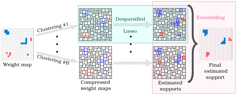
Computationally, to derive the EnCluDL solution we must solve $B$ independent CluDL problems, making the global problem embarrassingly parallel; nevertheless, we could run the CluDL algorithm on standard desktop stations without parallelization with $n=400$, $p\approx 10^{5}$, $C=500$ and $B=25$ in less than $10$ minutes. Note that, the clustering step being much quicker than the inference step, $p$ has a very limited impact on the total computation time.

The complexity for solving the Lasso depends significantly on the choice of solver, we then give the complexity in numbers of Lasso. The complexity for solving EnCluDL is given by the complexity of the resolution of $\mathcal{O}(B\times C)$ Lasso problems with $n$ samples and $C$ covariates, i.e., with clustering. It is noteworthy that the complexity for solving the desparsified Lasso on the original problem is given by the complexity of the resolution of $\mathcal{O}(p)$ Lasso problems with $n$ samples and $p$ covariates, i.e., without clustering. Then, EnCluDL should be much faster than the desparsified Lasso whenever $p\gg C$.

Appendix D Complementary simulation results

Figure 6: Results for various simulation parameters. The green line with circles correspond to the knockoffs, the brown line with triangle is the desparsified lasso, the dashed blue lines are for EnCluDL with length of the dashes increasing when $C$ diminishes: large dashes are for $C=100$, medium for $C=200$, small for $C=300$, tiny for $C=400$. We compute the same FWER and TPR quantities as in Figure 4, and the same $80\%$ confidence intervals: by Binomial approximation for the FWER and taking first and last deciles for the TPR.

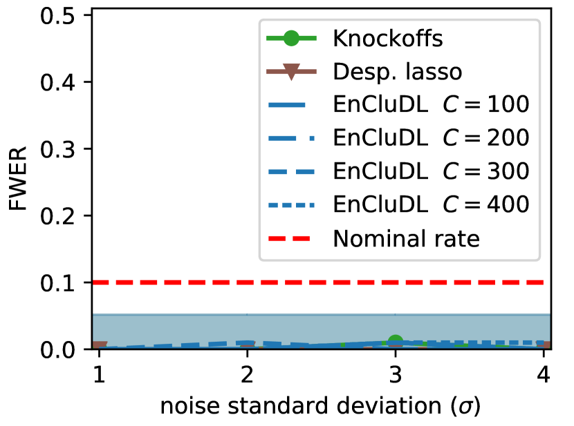
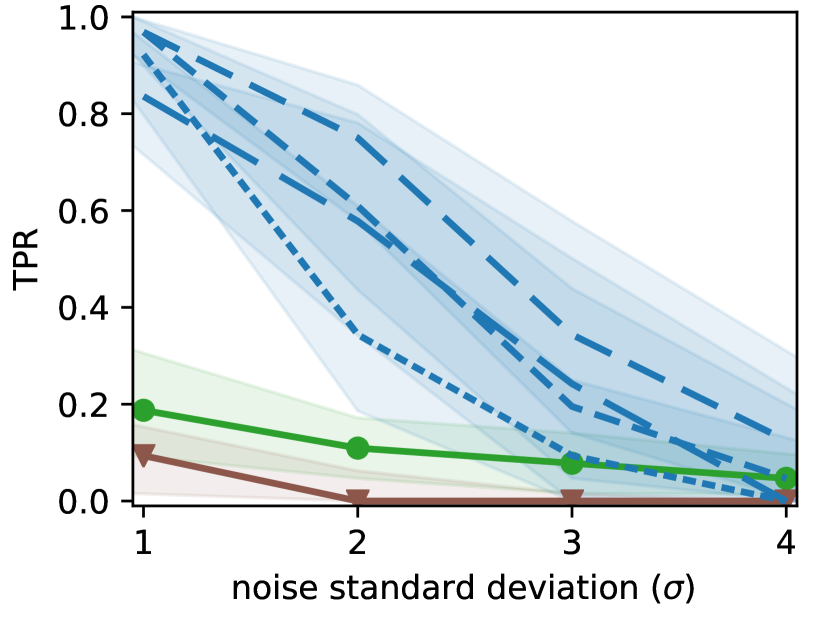
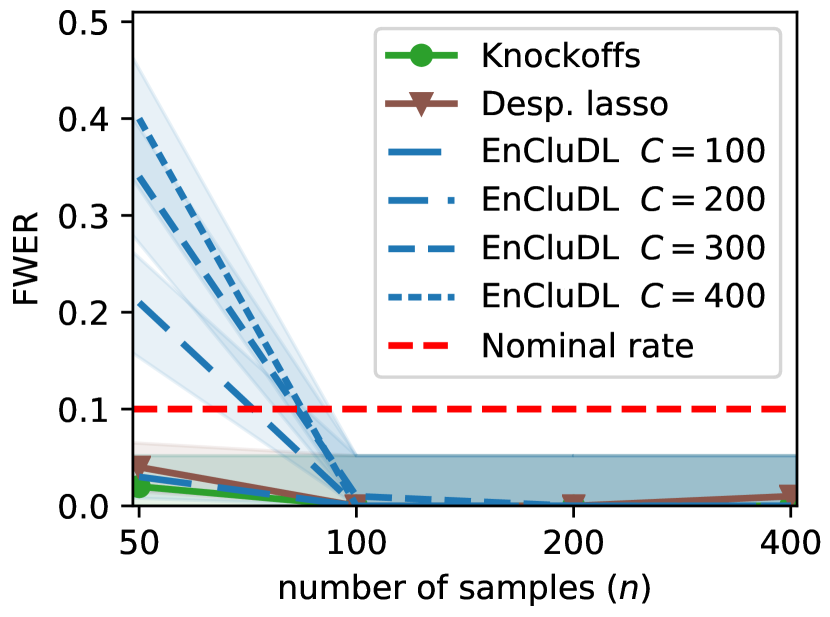
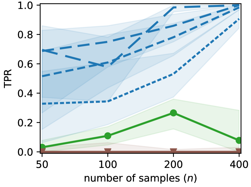
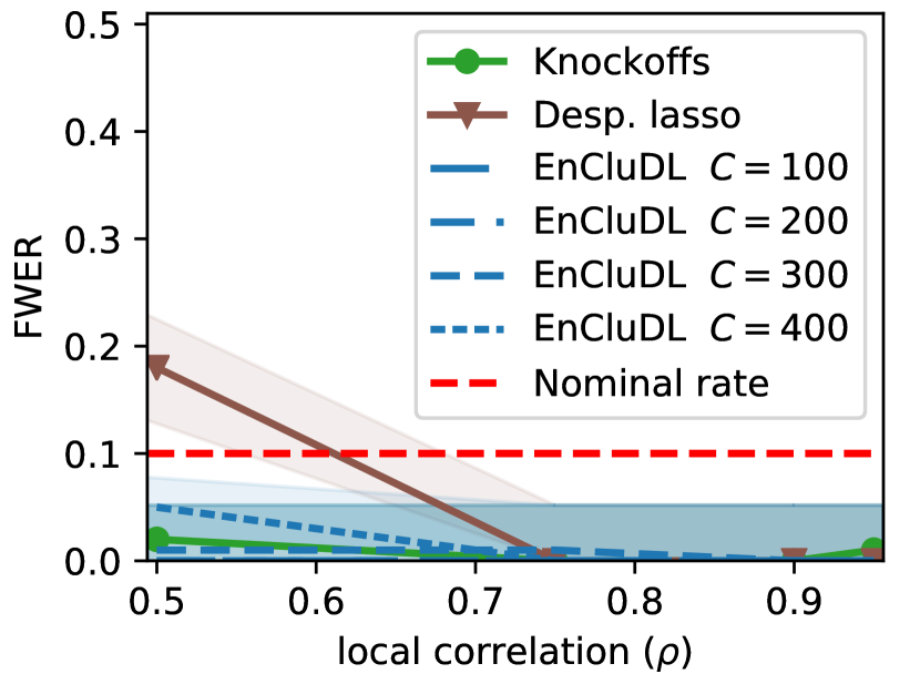
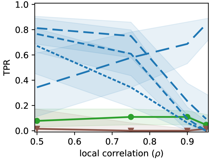
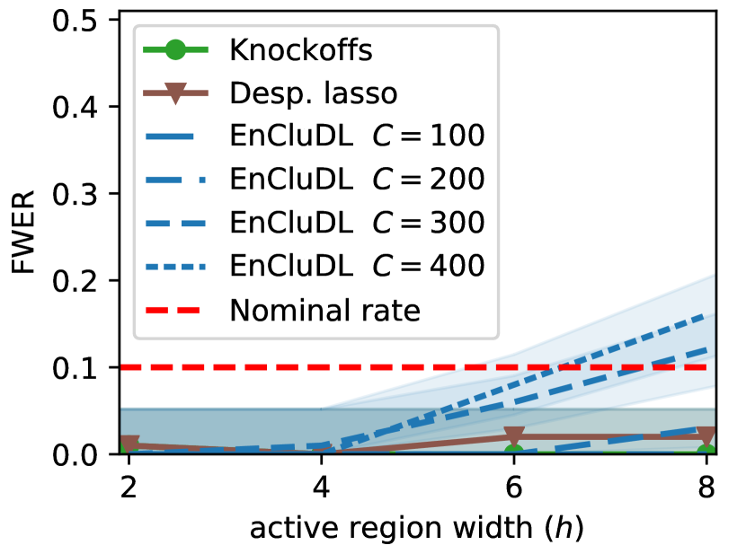
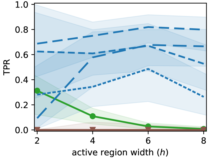
In Figure 6, we study the influence of the simulation parameters by varying one parameter of the central scenario at a time. We vary the noise standard deviation, the number of samples, the local correlation and the size of the support. For a better readability of the figures, we do not analyze the results of CLuDL since it is expected to be always a bit less powerful than EnCluDL while showing a similar behavior. First, we look at the plots where we vary the noise standard deviation $\sigma$. We observe that the methods reach the targeted FWER control and notice that EnCluDL benefits more strongly from the decrease of $\sigma$ regarding support recovery. Second, we analyze the results for various sample sizes ($n$) values. Concerning EnCluDL, we notice that the $\delta$-FWER is not controlled when $n=50$ except for $C=100$. This is not surprising since the $\delta$-FWER control is asymptotic and $n=50$ is not sufficient. In terms of support recovery, the problem gets easier with larger $n$, but only EnCluDL benefits strongly from an increase of $n$. Third, we investigate the influence of the level of correlation between neighboring covariates ($\rho$). Regarding FWER control, desparsified lasso does not control the FWER when $\rho=0.5$. Regarding the statistical power of EnCluDL, as one would expect, when the spatial structure is strong i.e., $\rho>0.9$, it is relevant to pick larger clusters, i.e., to take a smaller $C$. Indeed, to make a relevant choice for $C$, data structure has to be taken into account to derive good covariates’ clustering; this is true up to the limit given by the desired spatial tolerance. A good clustering creates clusters that are weakly correlated and contains covariates that are highly correlated. This observation is linked to assumption ($ii$) of Proposition 4.1 or to assumption ($ii.a$) and ($ii.b$) of Proposition B.1. Finally, we consider the results for different support sizes coded by the active region width $h$. Sparsity is a crucial assumption for desparsified lasso and then for EnCluDL. Also, when $p$ (or $C$) increases the required sparsity is greater. This explains why when $h=8$ and $C\geq 300$, the empirical $\delta$-FWER is slightly above the expected nominal rate. Regarding the statistical power of EnCluDL, as one could expect, when the active regions are large, it is relevant to use large clusters. However, it can be difficult to estimate this parameter in advance, thus we prefer to consider desired spatial tolerance parameter $\delta$ and data structure to set $C$.

Appendix E Proofs

E.1 Proof of Proposition 4.1 and Proposition B.1

First, we start by the proof of Proposition 4.1 which is derived from Bühlmann et al. [2013, Proposition 4.3]:

Proof.

With assumption $(ii)$ and Bühlmann et al. [2013, Proposition 4.3], we have, for all $c\in[C]$:

$$\bm{\theta}_{c}^{*}=|G_{c}|\sum_{j\in G_{c}}w_{j}\bm{\beta}^{*}_{j}\enspace,$$

where, for all $j\in G_{c}$:

$$w_{j}=\frac{\sum_{k\in G_{c}}\bm{\Sigma}_{j,k}}{\sum_{k\in G_{c}}\sum_{k^{\prime}\in G_{c}}\bm{\Sigma}_{k,k^{\prime}}}\enspace.$$

From assumption $(i)$, we have $w_{j}>0$ for all $j\in G_{c}$. Assumption $(iii)$ ensures that, for all $j\in G_{c}$, the $\bm{\beta}^{*}_{j}$ have the same sign. Then, $\bm{\theta}_{c}^{*}$ is of the same sign as the $\bm{\beta}^{*}_{j}$ and is non-zero only if there exists $j\in G_{c}$ such that $\bm{\beta}^{*}_{j}\neq 0$. ∎

Now, we give the proof of Proposition B.1 which is mainly derived from Bühlmann et al. [2013, Proposition 4.4]:

Proof.

With assumption $(ii.a)$ and $(ii.b)$ and Bühlmann et al. [2013, Proposition 4.4], we have, for all $c\in[C]$:

$$\bm{\theta}_{c}^{*}=|G_{c}|\sum_{j\in G_{c}}w^{\prime}_{j}\bm{\beta}^{*}_{j}+\bm{\kappa}_{c}\enspace,$$

where

$$w^{\prime}_{j}=\frac{\sum_{k\in G_{c}}\operatorname{Cov}(\mathbf{X}_{.,j},\mathbf{X}_{.,k}~{}|~{}\{\mathbf{Z}_{.,c^{\prime}}:c^{\prime}\neq c\})}{\sum_{k\in G_{c}}\sum_{k^{\prime}\in G_{c}}\operatorname{Cov}(\mathbf{X}_{.,k},\mathbf{X}_{.,k^{\prime}}~{}|~{}\{\mathbf{Z}_{.,c^{\prime}}:c^{\prime}\neq c\})}\enspace,$$

and, for all $c\in[C]$

$$|\bm{\kappa}_{c}|\leq(\bm{\nu}_{c}~{}/ \bm{\tau}_{c})\lVert{\bm{\beta}^{*}}\rVert_{1}\enspace.$$

Let us define $\tilde{\bm{\theta}}$ by

$$\tilde{\bm{\theta}}_{c}=|G_{c}|\sum_{j\in G_{c}}w^{\prime}_{j}\bm{\beta}^{*}_{j}\enspace.$$

Then,

$$\bm{\theta}^{*}=\tilde{\bm{\theta}}+\bm{\kappa}\enspace,$$

And, similarly as in the proof of Proposition 4.1, from assumption $(i)$ and $(iii)$, $\tilde{\bm{\theta}}_{c}$ is of the same sign as the $\bm{\beta}^{*}_{j}$ for $j\in G_{c}$ and is non-zero only if there exists $j\in G_{c}$ such that $\bm{\beta}^{*}_{j}\neq 0$. ∎

E.2 Proof of Proposition 4.2

Before going trough the proof of Proposition 4.2, we introduce the grouping function $g$ that matches the covariate index to its corresponding group index:

$$\begin{split}g:[p]&\to[C]\\ ~{}j~{}&\mapsto~{}c~{}\quad\operatorname{if}~{}j\in G_{c}\enspace.\\ \end{split}$$

Then, Equation 7 can be rewritten as follows:

$$\begin{split}&\text{for all}~{}j\in[p],\quad\hat{p}_{j}=\hat{p}^{\mathcal{G}}_{g(j)}\enspace,\\ &\text{for all}~{}j\in[p],\quad\hat{q}_{j}=\hat{q}^{\mathcal{G}}_{g(j)}\enspace.\\ \end{split}$$ (18)

Proof.

(i) Suppose that we are under $H^{\delta}_{0}(j)$. Since the cluster diameters are all smaller than $\delta$, all the covariates in $G_{g(j)}$ have a corresponding weight equal to zero. Thus, using Proposition 4.1, we have $\bm{\theta}_{g(j)}^{*}=0$, i.e., we are under $H_{0}(G_{g(j)})$. Under this last null-hypothesis, using Equation 11 and Equation 18, we have:

$$\text{for all}~{}\alpha\in(0,1),~{}\mathbb{P}(\hat{p}_{g(j)}^{\mathcal{G}}\leq\alpha)=\mathbb{P}(\hat{p}_{j}\leq\alpha)=\alpha\enspace.$$

This last result being true for any $j\in N^{\delta}$, we have shown that the elements of the family $\hat{p}$ control the $\delta$-type 1 error.

(ii) As mentioned in Section 4.4, we know that, the family $\hat{q}^{\mathcal{G}}$ controls the FWER, i.e., for $\alpha\in(0,1)$ we have $\mathbb{P}(\min_{c\in N_{\mathcal{G}}}\hat{q}^{\mathcal{G}}_{c}\leq\alpha)\leq\alpha$. Let us denote by $g^{-1}(N_{\mathcal{G}})$ the set of indexes of covariates that belong to the groups of $N_{\mathcal{G}}$, i.e., $g^{-1}(N_{\mathcal{G}})=\left\{j\in[p]:{g(j)}\in N_{\mathcal{G}}\right\}$. Again, given that all the cluster diameters are smaller than $\delta$ and using Proposition 4.1, if $j\in N^{\delta}$ then $g(j)\in N_{\mathcal{G}}$. That is to say $N^{\delta}\subset g^{-1}(N_{\mathcal{G}})$. Then, we have:

$$\min_{j\in N^{\delta}}(\hat{q}_{j})\geq\min_{j\in g^{-1}(N_{\mathcal{G}})}(\hat{q}_{j})\enspace.$$

We can also notice that:

$$\begin{split}\min_{j\in g^{-1}(N_{\mathcal{G}})}(\hat{q}_{j})&=\min_{j\in g^{-1}(N_{\mathcal{G}})}(\hat{q}^{\mathcal{G}}_{g(j)})\\ &=\min_{g(j)\in N_{\mathcal{G}}}(\hat{q}^{\mathcal{G}}_{g(j)})\enspace.\\ \end{split}$$

Replacing $g(j)\in[C]$ by $c\in[C]$, and using Equation 6, we obtain:

$$\text{for all}~{}\alpha\in(0,1),~{}\mathbb{P}(\min_{j\in N^{\delta}}(\hat{q}_{j})\leq\alpha)\leq\mathbb{P}(\min_{c\in N_{\mathcal{G}}}\hat{q}^{\mathcal{G}}_{c}\leq\alpha)\leq\alpha\enspace.$$

This last result states that the family $(\hat{q}_{j})_{j\in[p]}$ controls the $\delta$-FWER. ∎

E.3 Proof of Proposition 4.3

The proof of Proposition 4.3 is inspired by the one proposed by Meinshausen et al. [2009]. However, it is subtly different since we can not remove the term $\min_{j\in N^{\delta}}$ and have to work with it to obtained the desired inequality. First, we start by making a short remark about the $\gamma$-quantile quantity.

Definition E.1 (empirical $\gamma\mbox{-quantile}$).

For a set $V$ of real numbers and $\gamma\in(0,1)$, let

$$\gamma\mbox{-quantile}(V)=\min\left\{v\in V:\frac{1}{|V|}\sum_{w\in V}\mathds{1}_{w\leq v}\geq\gamma\right\}\enspace.$$ (19)

Remark E.1.

For a set of real number $V$ and for $a\in\mathbb{R}$, let us define the quantity $\pi(a,V)$ by the following:

$$\pi(a,V)=\frac{1}{|V|}\sum_{v\in V}\mathds{1}\left(v\leq a\right)$$ (20)

Then, for $\gamma\in(0,1)$, the two events $E_{1}=\{\pi(a,V)\geq\gamma\}$ and $E_{2}=\{\gamma\mbox{-quantile}(V)\leq a\}$ are identical.

Now, we give the proof of Proposition 4.3.

Proof.

First, one can notice that, from Equation 8, we have:

$$\min_{j\in N^{\delta}}(\tilde{q}_{j}(\gamma))\geq\min\left\{1,\gamma\mbox{-quantile}\left(\left\{\min_{j\in N^{\delta}}\left(\frac{\hat{q}^{(b)}_{j}}{\gamma}\right):b\in[B]\right\}\right)\right\}\enspace.$$

Then, for $\alpha\in(0,1)$:

$$\begin{split}\mathbb{P}\left(\min_{j\in N^{\delta}}(\tilde{q}_{j}(\gamma))\leq\alpha\right)&\leq\mathbb{P}\left(\min\left\{1,\gamma\mbox{-quantile}\left(\left\{\min_{j\in N^{\delta}}\left(\frac{\hat{q}^{(b)}_{j}}{\gamma}\right):b\in[B]\right\}\right)\right\}\leq\alpha\right)\\ &=\mathbb{P}\left(\gamma\mbox{-quantile}\left(\left\{\min_{j\in N^{\delta}}\left(\frac{\hat{q}^{(b)}_{j}}{\gamma}\right):b\in[B]\right\}\right)\leq\alpha\right)\enspace.\\ \end{split}$$

Using Remark E.1, for $\gamma\in(0,1)$, with:

$$V=\left\{\min_{j\in N^{\delta}}\left(\frac{\hat{q}^{(b)}_{j}}{\gamma}\right):b\in[B]\right\}\quad\operatorname{and}\quad a=\alpha\enspace,$$

and noticing that:

$$\pi\left(\alpha,\left\{\min_{j\in N^{\delta}}\left(\frac{\hat{q}^{(b)}_{j}}{\gamma}\right):b\in[B]\right\}\right)=\frac{1}{B}\sum^{B}_{b=1}\mathds{1}\left\{\min_{j\in N^{\delta}}({\hat{q}^{(b)}_{j}})\leq\alpha\gamma\right\}\enspace,$$

then, we have:

$$\mathbb{P}\left(\gamma\mbox{-quantile}\left(\left\{\min_{j\in N^{\delta}}\left(\frac{\hat{q}^{(b)}_{j}}{\gamma}\right):b\in[B]\right\}\right)\leq\alpha\right)=\mathbb{P}\left(\frac{1}{B}\sum^{B}_{b=1}\mathds{1}\left\{\min_{j\in N^{\delta}}({\hat{q}^{(b)}_{j}})\leq\alpha\gamma\right\}\geq\gamma\right).$$

Then, the Markov inequality gives:

$$\mathbb{P}\left(\frac{1}{B}\sum^{B}_{b=1}\mathds{1}\left\{\min_{j\in N^{\delta}}({\hat{q}^{(b)}_{j}})\leq\alpha\gamma\right\}\geq\gamma\right)\leq\frac{1}{\gamma}\mathbb{E}\left[\frac{1}{B}\sum^{B}_{b=1}\mathds{1}\left\{\min_{j\in N^{\delta}}({\hat{q}^{(b)}_{j}})\leq\alpha\gamma\right\}\right]\enspace.$$

Then, using the assumption that the $B$ families $(\hat{q}^{(b)}_{j})_{j\in[p]}$ control of the $\delta$-FWER (last inequality), we have:

$$\frac{1}{\gamma}\mathbb{E}\left[\frac{1}{B}\sum^{B}_{b=1}\mathds{1}\left\{\min_{j\in N^{\delta}}({\hat{q}^{(b)}_{j}})\leq\alpha\gamma\right\}\right]=\frac{1}{\gamma}\frac{1}{B}\sum^{B}_{b=1}\mathbb{P}\left(\min_{j\in N^{\delta}}(\hat{q}^{(b)}_{j})\leq\alpha\gamma\right)\leq\alpha\enspace.$$

Finally, we have shown that, for $\alpha\in(0,1)$:

$$\mathbb{P}\left(\min_{j\in N^{\delta}}(\tilde{q}_{j}(\gamma))\leq\alpha\right)\leq\alpha\enspace.$$

This establishes that the family $(\tilde{q}_{j}(\gamma))_{j\in[p]}$ controls the $\delta$-FWER. ∎

E.4 Proof of Theorem 4.1

To show Theorem 4.1, we connect the previous results: Proposition 4.1, Proposition 4.2 and Proposition 4.3. First, we prove that clustered inference algorithms produce a p-value family that controls the $\delta$-FWER.

Proof.

Assuming the noise model Equation 1, assuming that Assumption 2.1 and Assumption 2.2 are verified for a distance parameter larger than $\delta$ and that the clustering diameter is smaller than $\delta$, then we directly obtain the assumption $(i)$ and $(iii)$ of Proposition 4.1. This means that the compressed representation has the correct pattern of non-zero coefficients, in particular it does not include in the support clusters of null-only covariates. Additionally, if one is able to perform a valid statistical inference on the compressed model Equation 3, i.e., to produce cluster-wise p-values such that Equation 4 holds, then Proposition 4.2 ensures that the p-value family constructed using the de-grouping method presented in Equation 7 controls the $\delta$-FWER. ∎

Now, we prove that ensembled clustered inference algorithms produce a p-value family that controls the $\delta$-FWER.

Proof.

Given the above arguments, the p-value families produced by clustered inference algorithms subject to all clusterings fulfilling the theorem hypotheses control the $\delta$-FWER. Then, using the aggregation method given by Equation 8, we know from Proposition 4.3 that the aggregated p-value family also controls the $\delta$-FWER. ∎

References

- Bach [2008] F. R. Bach. Bolasso: model consistent lasso estimation through the bootstrap. In Proceedings of the 25th international conference on Machine learning, pages 33–40, 2008.
- Balding [2006] D. J. Balding. A tutorial on statistical methods for population association studies. Nature reviews genetics, 7(10):781–791, 2006.
- Barber and Candès [2015] R. F. Barber and E. Candès. Controlling the false discovery rate via knockoffs. Ann. Statist., 43(5):2055–2085, 10 2015.
- Bellec and Zhang [2019] P. C. Bellec and C.-H. Zhang. De-biasing the lasso with degrees-of-freedom adjustment. arXiv preprint arXiv:1902.08885, 2019.
- Benjamini and Hochberg [1995] Y. Benjamini and Y. Hochberg. Controlling the False Discovery Rate: A Practical and Powerful Approach to Multiple Testing. J. R. Stat. Soc. Ser. B Stat. Methodol., 57(1):289–300, 1995.
- Berk et al. [2013] R. Berk, L. Brown, A. Buja, K. Zhang, and L. Zhao. Valid post-selection inference. Ann. Statist., 41(2):802–837, 2013.
- Blanchard and Geman [2005] G. Blanchard and D. Geman. Hierarchical testing designs for pattern recognition. The Annals of Statistics, 33(3):1155–1202, 2005.
- Bühlmann [2013] P. Bühlmann. Statistical significance in high-dimensional linear models. Bernoulli, 19(4):1212–1242, 09 2013.
- Bühlmann et al. [2013] P. Bühlmann, P. Rütimann, S. van de Geer, and C.-H. Zhang. Correlated variables in regression: Clustering and sparse estimation. Journal of Statistical Planning and Inference, 143(11):1835 – 1858, 2013.
- Candès et al. [2018] E. Candès, Y. Fan, L. Janson, and J. Lv. Panning for gold:‘model-X’ knockoffs for high dimensional controlled variable selection. J. R. Stat. Soc. Ser. B Stat. Methodol., 80(3):551–577, 2018.
- Celentano et al. [2020] M. Celentano, A. Montanari, and Y. Wei. The lasso with general gaussian designs with applications to hypothesis testing. arXiv preprint arXiv:2007.13716, 2020.
- Chatterjee and Lahiri [2011] A. Chatterjee and S. N. Lahiri. Bootstrapping lasso estimators. J. Amer. Statist. Assoc., 106(494):608–625, 2011.
- Cheng et al. [2020] D. Cheng, Z. He, A. Schwartzman, et al. Multiple testing of local extrema for detection of change points. Electron. J. Stat., 14(2):3705–3729, 2020.
- Chevalier et al. [2018] J.-A. Chevalier, J. Salmon, and B. Thirion. Statistical inference with ensemble of clustered desparsified lasso. In International Conference on Medical Image Computing and Computer-Assisted Intervention, pages 638–646. Springer, 2018.
- Chevalier et al. [2020] J.-A. Chevalier, A. Gramfort, J. Salmon, and B. Thirion. Statistical control for spatio-temporal meg/eeg source imaging with desparsified multi-task lasso. In Thirty-fourth Conference on Neural Information Processing Systems, 2020.
- Chevalier et al. [2021] J.-A. Chevalier, T.-B. Nguyen, J. Salmon, G. Varoquaux, and B. Thirion. Decoding with confidence: Statistical control on decoder maps. NeuroImage, page 117921, 2021.
- De Martino et al. [2008] F. De Martino, G. Valente, N. Staeren, J. Ashburner, R. Goebel, and E. Formisano. Combining multivariate voxel selection and support vector machines for mapping and classification of fMRI spatial patterns. Neuroimage, 43(1):44–58, 2008.
- Dehman et al. [2015] A. Dehman, C. Ambroise, and P. Neuvial. Performance of a blockwise approach in variable selection using linkage disequilibrium information. BMC bioinformatics, 16(1):148, 2015.
- Dezeure et al. [2015] R. Dezeure, P. Bühlmann, L. Meier, and N. Meinshausen. High-dimensional inference: Confidence intervals, -values and R-Software hdi. Statist. Sci., 30(4):533–558, 2015.
- Dezeure et al. [2017] R. Dezeure, P. Bühlmann, and C.-H. Zhang. High-dimensional simultaneous inference with the bootstrap. Test, 26(4):685–719, 2017.
- Dunn [1961] O. J. Dunn. Multiple comparisons among means. J. Amer. Statist. Assoc., 56(293):52–64, 1961.
- Gimenez and Zou [2019] J. R. Gimenez and J. Zou. Discovering conditionally salient features with statistical guarantees. International Conference on Machine Learning, pages 2290–2298, 2019.
- Hoyos-Idrobo et al. [2018] A. Hoyos-Idrobo, G. Varoquaux, J. Kahn, and B. Thirion. Recursive nearest agglomeration (rena): fast clustering for approximation of structured signals. IEEE transactions on pattern analysis and machine intelligence, 41(3):669–681, 2018.
- Janson and Su [2016] L. Janson and W. Su. Familywise error rate control via knockoffs. Electron. J. Stat., 10(1):960–975, 2016.
- Javanmard and Montanari [2014] A. Javanmard and A. Montanari. Confidence intervals and hypothesis testing for high-dimensional regression. J. Mach. Learn. Res., 15:2869–2909, 2014.
- Javanmard and Montanari [2018] A. Javanmard and A. Montanari. Debiasing the lasso: Optimal sample size for Gaussian designs. Ann. Statist., 46(6A):2593–2622, 2018.
- Lee et al. [2016] J. Lee, D. Sun, Y. Sun, and J. Taylor. Exact post-selection inference, with application to the lasso. Ann. Statist., 44(3):907–927, 2016.
- Liu and Yu [2013] H. Liu and B. Yu. Asymptotic properties of lasso+ mls and lasso+ ridge in sparse high-dimensional linear regression. Electron. J. Stat., 7:3124–3169, 2013.
- Liu and Janson [2020] M. Liu and L. Janson. Fast and powerful conditional randomization testing via distillation. arXiv preprint arXiv:2006.03980, 2020.
- Lockhart et al. [2014] R. Lockhart, J. Taylor, R. J. Tibshirani, and R. Tibshirani. A significance test for the lasso. Ann. Statist., 42(2):413, 2014.
- Mandozzi and Bühlmann [2016] J. Mandozzi and P. Bühlmann. Hierarchical testing in the high-dimensional setting with correlated variables. J. Amer. Statist. Assoc., 111(513):331–343, 2016.
- Meinshausen [2008] N. Meinshausen. Hierarchical testing of variable importance. Biometrika, 95(2):265–278, 2008.
- Meinshausen [2015] N. Meinshausen. Group bound: confidence intervals for groups of variables in sparse high dimensional regression without assumptions on the design. J. R. Stat. Soc. Ser. B Stat. Methodol., pages 923–945, 2015.
- Meinshausen and Bühlmann [2010] N. Meinshausen and P. Bühlmann. Stability selection. J. R. Stat. Soc. Ser. B Stat. Methodol., 72:417–473, 2010.
- Meinshausen et al. [2009] N. Meinshausen, L. Meier, and P. Bühlmann. P-values for high-dimensional regression. J. Amer. Statist. Assoc., 104(488):1671–1681, 2009.
- Minnier et al. [2011] J. Minnier, L. Tian, and T. Cai. A perturbation method for inference on regularized regression estimates. J. Amer. Statist. Assoc., 106(496):1371–1382, 2011.
- Mitra and Zhang [2016] R. Mitra and C.-H. Zhang. The benefit of group sparsity in group inference with de-biased scaled group lasso. Electron. J. Stat., 10(2):1829–1873, 2016.
- Ndiaye et al. [2017] E. Ndiaye, O. Fercoq, A. Gramfort, V. Leclère, and J. Salmon. Efficient smoothed concomitant lasso estimation for high dimensional regression. In Journal of Physics: Conference Series, volume 904, page 012006. IOP Publishing, 2017.
- Nguyen et al. [2019] T.-B. Nguyen, J.-A. Chevalier, and B. Thirion. Ecko: Ensemble of clustered knockoffs for robust multivariate inference on fMRI data. In International Conference on Information Processing in Medical Imaging, pages 454–466. Springer, 2019.
- Nguyen et al. [2020] T.-B. Nguyen, J.-A. Chevalier, B. Thirion, and S. Arlot. Aggregation of multiple knockoffs. In International Conference on Machine Learning, pages 7283–7293. PMLR, 2020.
- Ning and Liu [2017] Y. Ning and H. Liu. A general theory of hypothesis tests and confidence regions for sparse high dimensional models. Ann. Statist., 45(1):158–195, 2017.
- Norman et al. [2006] K. A. Norman, S. M. Polyn, G. J. Detre, and J. V. Haxby. Beyond mind-reading: multi-voxel pattern analysis of fMRI data. Trends in cognitive sciences, 10(9):424–430, 2006.
- Park et al. [2006] M. Y. Park, T. Hastie, and R. Tibshirani. Averaged gene expressions for regression. Biostatistics, 8(2):212–227, 05 2006.
- Reid et al. [2016] S. Reid, R. Tibshirani, and J. Friedman. A study of error variance estimation in lasso regression. Statistica Sinica, pages 35–67, 2016.
- Richards et al. [2009] J.W. Richards, P.E. Freeman, A.B. Lee, and C.M. Schafer. Exploiting low-dimensional structure in astronomical spectra. The Astrophysical Journal, 691(1):32, 2009.
- Tibshirani [1996] R. Tibshirani. Regression shrinkage and selection via the lasso. J. R. Stat. Soc. Ser. B Stat. Methodol., 58(1):267–288, 1996.
- Tibshirani et al. [2016] R. J. Tibshirani, J. Taylor, R. Lockhart, and R. Tibshirani. Exact post-selection inference for sequential regression procedures. J. Amer. Statist. Assoc., 111(514):600–620, 2016.
- van de Geer et al. [2014] S. van de Geer, P. Bühlmann, Y. Ritov, and R. Dezeure. On asymptotically optimal confidence regions and tests for high-dimensional models. Ann. Statist., 42(3):1166–1202, 2014.
- Varoquaux et al. [2012] G. Varoquaux, A. Gramfort, and B. Thirion. Small-sample brain mapping: sparse recovery on spatially correlated designs with randomization and clustering. In International Conference on Machine Learning, 2012.
- Wainwright [2009] M. J. Wainwright. Sharp thresholds for high-dimensional and noisy sparsity recovery using -constrained quadratic programming (lasso). IEEE Trans. Image Process., 55(5):2183–2202, 2009.
- Wasserman and Roeder [2009] L. Wasserman and K. Roeder. High-dimensional variable selection. Ann. Statist., 37(5A):2178–2201, 2009.
- Westfall and Young [1993] P. H. Westfall and S. S. Young. Resampling-based multiple testing: Examples and methods for p-value adjustment, volume 279. John Wiley & Sons, 1993.
- Yu and Bien [2019] G. Yu and J. Bien. Estimating the error variance in a high-dimensional linear model. Biometrika, 106(3):533–546, 2019.
- Zhang and Zhang [2014] C.-H. Zhang and S. S. Zhang. Confidence intervals for low dimensional parameters in high dimensional linear models. J. R. Stat. Soc. Ser. B Stat. Methodol., 76(1):217–242, 2014.