remarkRemark \newsiamremarkhypothesisHypothesis \newsiamthmclaimClaim \newsiamremarkexampleExample \headersLocal Flux RecoveryC. He \externaldocumentsupplement
Flux recovery for Cut finite element method and its application in a posteriori error estimation ††thanks: This work was funded by the EPSRC grant EP/P01576X/1.
Abstract
In this article, we aim to recover locally conservative and conforming fluxes for the linear Cut Finite Element Solution with Nitsche’s method for Poisson problems with Dirichlet boundary condition. The computation of the conservative flux in the Raviart-Thomas space is completely local and does not require to solve any mixed problem. The -norm of the difference between the numerical flux and the recovered flux can then be used as a posteriori error estimator in the adaptive mesh refinement procedure. Theoretically we are able to prove the global reliability and local efficiency. The theoretical results are verified in the numerical results. Moreover, in the numerical results we also observe optimal convergence rate for the flux error.
keywords:
CutFEM, a Posteriori Error Estimation, Flux Recovery, Adaptive Mesh Refinement68Q25, 68R10, 68U05
1 Introduction
Cut finite element method (CutFEM) may be regarded as a fictitious domain method. The finite element fictitious domain method was introduced in [28] as an approach to simplify the meshing problem and then further improved in [8, 31, 14, 5, 30]. The challenges for such methods are typically that if the mesh is cut in an unfavorable way the system can be ill-conditioned and accuracy can be lost. Several approaches have been proposed to handle this problem, all based on the idea of extending the stability of the solution in the bulk up to the boundary. In [31], boundary fluxes are evaluated using the gradient extended from internal elements. In [33, 32, 13, 4], agglomeration of adjacent elements is used. Finally, in [12, 15], the weakly consistent ghost penalty term was proposed that serves purpose.
The purpose of this paper is to design and analyze a locally conservative flux in the Raviart-Thomas space of order and for the linear CutFEM. We will base our discussion on the approximation of Poisson’s problem [15] in two dimensions. In addition, the CutFEM uses Nitsche’s method [37] to impose Dirichlet boundary conditions and a ghost penalty term [12] to enhance stability in the boundary zone.
One important application for the flux recovery is that the -norm of the difference between the numerical flux and the recovered flux can be used in the a posteriori error estimation. The main motivation for studying the a posteriori error estimation is the application of adaptive mesh refinement (AMR) procedure. It is well known that AMR is extremely useful for problems with singularities, discontinuities, sharp derivatives etc.. And it has been extensively studied in the last several decades, see e.g., [40, 3]. In [17], a residual based a posterior error estimator for the CutFEM method was studied. One drawback of residual based error estimation is that its reliability constants are unknown and usually not polynomial-robust and problem dependent. On the other hand, it is well known that the difference between the numerical flux and a locally conservative (equilibrate) flux automatically yields an upper bound for the true energy error with a reliability constant being exactly .
Thanks to the sharp reliability, equilibrate flux recovery has been extensively studied for various finite element methods on fitted meshes in the last decade. It is well known that for discontinuous Galerkin methods, a locally element-wise equilibrate flux can be easily obtained thanks to the fact that the test functions are completely local [6, 24, 1, 10, 7]. For nonconforming finite element methods of odd order, a local element–wise construction can be also easily obtained by taking advantage of the nonconforming local basis functions [35, 19]. For second order nonconforming finite element method, an explicit construction is designed in [34]. However, for nonconforming methods of general even orders and conforming finite element methods, local element-wise (explicit) flux recovery is not straightforward and usually local problems on star patches need to be solved [2, 25, 7]. In [38], a conservative flux is obtained by adding a piecewise constant correction through minimizing a weighted global -norm.
We note that the method introduced in [7] is applicable to various finite element methods, and furthermore, designed in a framework that fully takes advantages of the local basis functions for each method. For conforming finite elements on fitted meshes, this method only requires solving local problems that do not involve any hybrid mixed problem which are required e.g., in [11, 20, 25]. In this work, we use a similar approach for CutFEM. For the interior elements not cut by the boundary, the recovered flux is similar to that in [7] although it needs extra treatment for the ghost penalty term. Unlike the fitted methods whose mesh is an exact partition of the computational domain, one major challenge for cut finite elements is that the domain cuts the background mesh in an arbitrary fashion. For cut elements, the recovery of the flux becomes complex due to non-standard terms in the variational formulation and partial intersections between the mesh and the domain, and, therefore, needs to be carefully designed to avoid artificial error. We divide boundary elements into two types, i.e., the set of boundary elements that are fitted and not fitted to the mesh, and design the flux differently.
Contrary to the classical approach, we consider the domain with non-polygonal boundary. In order to achieve the same accuracy as the classical fitted method, boundary geometry and boundary data for CutFEM need to be approximated to similar accuracy. It is therefore important in this context to derive error estimators that are able to integrate both the discretization error of the method and the discretization error of the geometry. In this work, we approximate the physical geometry by a piecewise affine polygonal domain. In [17], a boundary correction error was separated that particularly estimates the geometry approximation error. The computation of this term, however, is not trivial and requires the construction of a sub mesh. Nevertheless, numerical results have shown that such error is not necessary to compute since the boundary approximation error can already be captured by the residual based error estimator in [17]. In this paper, we also discard such term and numerical results also confirm that our error estimator is able to catch both the boundary approximation errors and the discretization error due to the numerical method.
Although we herein restrict the discussion to the case of piecewise affine approximation spaces from [15], we believe that the ideas introduced can be extended for instance to the high order case discussed in [16] as regards the CutFEM method, and in [7] as regards the flux reconstruction in two dimensions. For other works treating a posteriori error estimation and cut cell techniques we refer to [26], where a finite volume method was considered, and [39] and [22] where cut cell methods were applied.
This paper is organized as follows. In Section 2, the model problem and the CutFEM are introduced. In Section 3, we design the local conservative flux by introducing an auxiliary mixed method and establish its well-posedness. In Section 4, we apply the conservative flux in the a posteriori error estimation and establish its reliability and efficiency. Finally, we show the results of several numerical experiments in Section 5.
2 Model problem and the Cut Finite Element Method
2.1 The continuous problem
Let be a domain in () with Lipschitz continuous, piecewise smooth boundary with exterior unit normal . We consider the problem: find such that
| (2.1) |
where and . For the sake of simplicity, we only consider the model problem of Laplacian operator with Dirichlet boundary conditions. However, the technique could be generalized to other boundary conditions and more complex elliptic operators.
Define the spaces
Then the weak formulation for this problem renders to find such that
where . It follows from the Lax-Milgram lemma that there exists a unique solution to this problem.
2.2 The mesh, discrete domain, and finite element spaces
Assume that is composed of a finite number of smooth surfaces , such that . We let be the signed distance function such that
where is the complement of the closure of . We define , be the tubular neighborhood of . Choose be the background domain (see e.g., the square outline of the entire mesh in Fig. 1) such that it is polygonal, and where is chosen such that is well defined in . Let be a partition of into shape regular triangles or tetrahedra (see e.g., the mesh in Fig. 1). Note that this setting allows meshes with locally dense refinement.
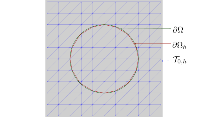
Given a subset of , let be the sub-mesh defined by
| (2.2) |
i.e., the sub-mesh consisting of elements that have non-zero intersection with , and let
| (2.3) |
which is the union of all elements in .
For each , let (see Fig. 1 for an example) be a polygonal domain approximating . We assume that , i.e., is within the distance of to . Moreover, we also require that the maximum distance between the two domains is small enough so that is a sufficiently good approximation to . More details will be given later.
Let the active mesh be defined by
| (2.4) |
i.e., the sub-mesh consisting of elements that intersect , and let
| (2.5) |
Since cut the active mesh in an arbitrary fashion, we denote by the set of elements that are “cut” by , i.e.,
We further assume that is constructed in such a way that for each , the intersection is a subset of a dimensional hyperplane, i.e., a line segment in two dimensions. Under the assumptions on , and if we also assume that is sufficiently small, then for any element there exists an element such that where denotes the Landau big-.
Also we denote by the set of all facets of , and by and the set of all interior and boundary facets with respect to , respectively. It is obvious that . For each denote by an unit vector normal to and by (or ) the diameter of . If , then is the outward unit normal vector. For each denote by the diameter of and by the set of all facets of .
On the boundary , let be the outer normal to . For each , we assume that, for small enough, there exist a vector function , , and , such that the function, , is well defined and satisfies for all . Here is the distance from the approximate to the physical boundary in the direction . The mapping allows us to impose the boundary data defined on the physical boundary on the approximate boundary. The existence of the vector-valued function is known to hold on Lipschitz domains, see Grisvard [29]. We further assume that
For convenience, we will drop the second argument, , of below whenever it takes the value and then denotes the map . Moreover, we assume that the following assumption is satisfied
| (2.6) |
The above assumption immediately implies that is within the distance of of , i.e.,
| (2.7) |
This assumption is necessary for the constant in the a posteriori error estimates to be independent of the geometry/mesh configuration see [17]. It is however not enough to guarantee the optimal a priori error estimates, which requires , and , see [16]. It is noted that in theory we can assume neither nor . However, for simplicity, we assume . This will help skip the analysis for the a posteriori error estimation on the part of data approximation error of . Such error can be eventually ignored in the computation since it is of higher order.
2.3 The Cut Finite Element Method
In this subsection we recall the CutFEM introduced in [15]. We begin with some necessary notation. For any , let and be those two elements sharing as a common facet such that the outer normal of coincides with . For any discontinuous function , define the jump of across the facet by
The set of facets associated with cut elements is defined by
The index above refers to the ghost penalization, defined on every .
For each , we define a sign function defined on such that
The conforming linear finite element space is then defined as
| (2.8) |
We also define the following forms:
| (2.9) |
where , , and are positive constants, is an approximation of defined on . A natural choice is that . Note that we only assumed that . In where is not originally defined, is defined to be an appropriate extension.
Remark 2.1.
Remark 2.2.
In order to guarantee the coercivity of the bilinear form in Eq. 2.9, has to be chosen large enough.
For , define the continuous and discrete energy norms respectively by
| (2.11) |
and
| (2.12) |
2.4 Some important inequalities
Below we list the well known trace and inverse inequalities [21, Section 1.4.3],
| (2.14) |
| (2.15) |
The following irregular trace inequality can be found in [30]
| (2.16) |
where the hidden constant is independent of the boundary-mesh intersection. Here and below we use the notation to denote less or equal up to a generic constant that is independent of the mesh-geometry configuration.
In the following Lemma, we also provide a Poincaré-type inequality for the boundary elements.
Lemma 2.3.
Let . Then for any such that or , there exists a local convex neighborhood of such that vanishes on a non-empty subset of and
| (2.17) |
where we defined outside using the trivial extension .
The proof of the lemma can be found in [17].
3 Mixed formulation
In this section, we introduce an auxiliary mixed formulation for the cut finite element method. The aim is not to solve the global mixed problem. Instead, our goal is to establish the connections between the mixed and CutFEM formulation, and, with the help of those connections, to locally recover a conservative flux in the space. The idea generates from [7] in which classical finite element methods with fitted meshes were studied.
Define the discontinuous finite element space on by
| (3.1) |
Also define the average operator:
We also denote by the set of all vertices in , and by and the sets of all interior and boundary vertices on . Obviously, we have . For each , define and be the sets of all elements and all facets sharing as a vertex, respectively. For each , we define a signed function on such that if is oriented counter-clockwise in , otherwise . We further define the following space:
Here is the space of linear functions defined on . For the sake of brevity, we use the following notations for piecewise integration,
where is a subset of . We now define semi-norms and norms on the discrete spaces defined above:
| (3.2) |
The auxiliary mixed formulation is defined as follows: find such that
| (3.3) |
where
| (3.4) |
where and is the set of vertices of . It is easy to check that the discrete kernel of coincides exactly with the CutFEM space, i.e.,
Indeed, any function in satisfies for any , and hence belongs to . Reciprocally, for any in , we can choose defined by for any , which yields and hence, . It is then obvious to see that the solution for Eq. 2.10 coincides with the solution for Eq. 3.3 if it is well defined.
3.1 Well-posedness of the mixed finite element approximation
Lemma 3.1 (continuity).
We have the following continuity results for the bilinear forms:
Proof 3.2.
The proof of the first assertion is trivial by Cauchy-Schwartz and the definitions of the norms:
As regards the second one, we first note that for any , so we clearly have that on , hence the continuity of . The remaining terms of are bounded as follows:
which ensures the continuity of .
Lemma 3.3 (inf-sup condition).
We also have the inf-sup result for the bilinear form:
| (3.5) |
where the constant is independent of the mesh size and domain-mesh intersection.
Proof 3.4.
We prove by construction. To define a linear function , it suffices to define for all and for all . For each , we let be the clockwise oriented elements in where is the number of elements in . We also let . We let . The rest are defined such that
| (3.6) |
It is easy to check that Eq. 3.6 is compatible. Moreover, it is easy to check that
| (3.7) |
For such that , we define in the same way (where we assume that has a boundary facet). Note that there are only interior facets in this case. And we also have
| (3.8) |
Finally, for such that , we simply put . Combining Eq. 3.7 and Eq. 3.8 gives that
| (3.9) |
We then have that
| (3.10) |
The last inequality follows from the equivalence of norms in a finite dimensional space. Immediately from Eq. 3.8, we also have the following bound:
| (3.11) |
By a direct computation, Eq. 3.11, and norm equivalence in a finite dimensional space, we have
| (3.12) |
Immediately, we also have, by using Eq. 2.16 for the last estimate,
| (3.13) |
We also have, thanks to Eq. 2.16,
| (3.14) |
Note that the involved constants do not depend on the interface-mesh intersection. Combing Eq. 3.12, Eq. 3.13 and Eq. 3.14 yields
| (3.15) |
Eq. 3.5 is then the direct consequence of Eq. 3.10 and Eq. 3.15. This completes the proof of the lemma.
By Eq. 2.13, we also have the uniform coercivity of on with respect to the norm .
Lemma 3.5.
Proof 3.6.
The proof is standard and follows from the Babuska-Brezzi theorem. We sketch the proof of the existence and uniqueness of the solution for the convenience of the readers. It is enough to show the uniqueness of the solution of the linear square system. We prove by contradiction. Assume both and are solutions to Eq. 3.3. From the second equation in Eq. 3.3, we have that . Then we have
By Eq. 2.13, we have . Then we have for all . Finally by the inf-sup condition Eq. 3.5, we obtain . Since the solution for Eq. 3.3 is unique, then the solution in Eq. 3.3 must coincide with the CutFEM solution of Eq. 2.10. This completes the proof of the lemma.
3.2 Local construction of
In this subsection, we aim to compute the solution to Eq. 3.3 based on the solution of Eq. 2.10 through solving local problems, following [7]. Firstly note that
| (3.16) |
Note that for any .
Let such that . We define on such that, for each ,
| (3.17) |
where denotes the barycentric basis function corresponding to the vertex . On , we impose that is null.
Recall from the definition of that the condition means that has to satisfy a constraint at any interior node. The last equation of Eq. 3.17 gives that for all and , so the constraint is obviously satisfied at the node , for . Hence, only has to satisfy the constraint equation at the node , for .
Also note that . It is then easy to check that the system introduced by Eq. 3.17 is compatible.
Lemma 3.7.
For any , the system Eq. 3.17 has a unique solution in .
Proof 3.8.
We first assume that . Because of the compatibility condition, the system Eq. 3.17 a one-dimensional kernel. Indeed, let defined on any by and
whereas on , we set . It is then easy to check that for all ,
| (3.18) |
Thus is the kernel of the system Eq. 3.17. However, it is obvious that does not satisfy the constraint equation for . Thus Eq. 3.17 has a unique solution under the constraint for . For , note that there are interior facets. The solution is then unique since there are unknowns with independent equations. This completes the proof of the lemma.
3.3 Computation of for
For each , recall that we let be the clockwise oriented elements in and is the number of elements in . When , we let . When , note that there are interior facets in . Also let denotes the other vertices of .
We firstly deal with the case . From the second equation in Eq. 3.17, it is easy to see that for . We then let
From the first equation in Eq. 3.17, a straight computation gives that
| (3.22) |
Note that we only used equations since the last one is linearly dependent. The constraint provides the last equation if :
| (3.23) |
Combining Eq. 3.22 and Eq. 3.23 yields a non-singular local system. It is helpful to denote the unknowns by , such that the matrix of the previous local system has constant coefficients and depends only on .
If , note that for , i.e., . Hence we can explicitly compute for . Thus no local problem is required to solve for boundary elements.
By a simple calculation, we also have the following estimate:
| (3.24) |
where and are the vectors in formed by and , respectively. Here denotes the Euclidean -norm.
We also obtain the following estimate for which will be used later. From the definition of , integration by parts, Eq. 2.16, and direct computations on norms of , we have
| (3.25) |
Immediately, we also have for any node that
| (3.26) |
3.4 Flux reconstruction
In this subsection, we locally recover a flux for each element . The element-wise construction is completely explicit and based on the computation of and . Denote the conforming Raviart-Thomas () space of index with respect to by
where . On a triangular element , a vector-valued function in is characterized by the following degrees of freedom (see Proposition 2.3.4 in [9]):
and
For each element , we define such that for all and for all and it satisfies:
| (3.27) |
where
Remark 3.11.
Remark 3.12.
Note that if , we then have that
We then define the global recovered flux by
| (3.28) |
Recall that on a cut element , is only defined on . We next introduce an extension of to the whole cut element . For each and , we extend to such that is linear and also satisfies that for all ,
| (3.29) |
Note that if the right-hand side is , this represents a zero extension.
Let be the projection operator onto the space defined on .
Lemma 3.13.
Proof 3.14.
By its definition, it is easy to see that . Firstly, we note that for all we have
| (3.31) |
since . To prove Eq. 3.30, we first consider the case of , i.e., , . Let such that and vanishes elsewhere. From Eq. 3.31 we have
| (3.32) |
By integration by parts, Eq. 3.27, the fact that , and Eq. 3.32, we have
| (3.33) |
which yields Eq. 3.30 for all interior elements.
Now consider the second case when . Again, let such that and vanishes elsewhere. From Eq. 3.31 we now have
| (3.34) |
Applying integration by parts on gives
| (3.35) |
which, combining with the following equation,
implies
| (3.36) |
Note that the previous relation also holds in the case .
Remark 3.15.
For the cut elements, it is not obvious to construct a flux that is both locally conservative in the cut part and, at the same time, maintains continuous normal flux. The technique of applying integration by parts in Eq. 3.36 renders the problem to be a more regular problem and completes partial elements to full elements.
4 Application in the a posteriori error estimation
For the sake of simplicity, we assume in this section that on any . In the adaptive procedure, we define the following local error indicators
| (4.1) |
and the corresponding estimators:
| (4.2) |
4.1 Reliability
Let be the lifting such that on and
Theorem 4.1 (Reliability).
Let be given by (3.28) and be the CutFEM solution in (2.10). We have the following reliability result:
| (4.3) |
where the constant is independent of the mesh size and mesh-domain intersection, and
Remark 4.2.
Thanks to the assumption that , we have that
Therefore both and could serve as the error estimator in the AMR procedure.
Proof 4.3.
By triangle inequality, we firstly have the following bound:
| (4.4) |
To bound we have
| (4.5) |
where we used (2.17) for the last inequality. This completes the proof of the theorem.
Remark 4.4.
It is useful to note that for any , we have that
| (4.6) |
Indeed, denoting by the values taken by at the vertices of and by the corresponding nodal basis functions on , we have using that ,
which yields the desired estimate.
Remark 4.5.
Remark 4.6.
From the above estimate, we observe that can be bounded by the classical residual based error estimator. Moreover, the constants are uniformly bounded and independent of the domain-mesh intersection. We further note that can also be bounded by with an additional higher order oscillation term,
Indeed, we could prove by equivalence of norms on finite dimensional space. Firstly note that implies . Therefore, based on the properties of , we have that for all and that in . Moreover, from the first equation in Eq. 3.27, we immediately have on for . From the second equation in Eq. 3.27, we have and thus, from Eq. 3.16, for each . Finally, the second equation in Eq. 3.25 implies on . Eventually, we have that implies , and, therefore, . In the numerical computation, we discard the term . is the so-called boundary correction error which we have thoroughly discussed in [17]. It was shown that adding such error does not affect the overall convergence rate as well as the final meshes when the mesh is fine enough.
4.2 Efficiency
Lemma 4.7.
Let be a given element in . Then the following local efficiency result holds:
| (4.8) |
where is a local neighborhood of that does not contain elements in and the efficiency constant does not depend on the mesh size nor the domain-mesh intersection.
Proof 4.8.
By the degrees of freedom for space, we have the following bound:
| (4.9) |
where is the projection onto the piecewise constant space on . Let and arbitrary, then from Eq. 3.27 we have:
| (4.10) |
The following lemma, which follows from theorem 4.5 in [17], gives the efficiency result for the irregular error terms. Define
where is the union of all elements sharing a common vertex with and .
Lemma 4.9.
We have the best approximation result for the irregular terms
| (4.16) |
where the constant does not depend on the mesh size nor the domain-mesh intersection and can be regarded as a higher order oscillation term.
Thanks to the previous result, we can easily deduce an error bound for the flux error , where .
Lemma 4.10.
Assume . Then one has:
| (4.17) |
Proof 4.11.
We have, using that , that
It is therefore sufficient to bound for any . For this purpose, we use Eq. 4.14. The triangle inequality together with norm equivalence in a discrete space and standard interpolation results give, for any , that:
| (4.18) |
where is the continuous, piecewise linear Lagrange interpolation operator. Together with Eq. 4.14, the second estimate of Eq. 4.15 and Lemma 4.9, this gives Eq. 4.17 which completes the proof of the lemma. Note that in the proof, we do not need the requirement that is piecewise linear.
5 Numerical results
In this section, we present several numerical examples to validate the performance of the a posteriori error estimator in the adaptive mesh refinement procedure. The adaptive mesh refinement procedure is set as follows:
For the penalty parameters in the finite element method, we set and . For the refinement strategy, we use the Dörfler marking strategy [23] and the refinement rate is set to be ten percent. Regarding the domain approximation, let be the level set function that satisfies on and negative (positive) inside (outside) the domain . Let be the nodal interpolation of with respect to . Then we define
| (5.1) |
We can easily check that Eq. 2.6 holds.
In the adaptive procedure, we compare the error estimators and defined in Eq. 4.2 with the residual based error estimator (see [17]) defined as follows,
| (5.2) |
The global residual based error estimator is then defined by
| (5.3) |
Example 5.1.
In this example, we test a problem with a strong interior peak. The exact solution has the following representation:
This function has a strong peak at the point .
Note that the boundary of the domain is regular, thus we have that . Moreover, the function value is very smooth and almost vanishes on the boundary. The purpose of this example is to test the efficacy of our adaptive algorithm for Nitsche’s method on a regular domain.
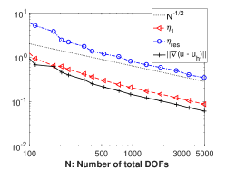
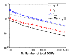
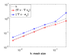
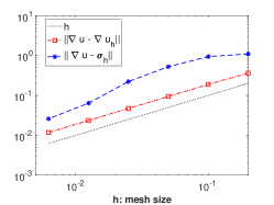
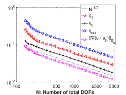
In the numerical scheme, and are approximated by their interpolations into the continuous piecewise linear space. We firstly test the convergence of the method on uniform meshes. The results are plotted in Fig. 2(e) which show optimal convergence rates (order ) for both the true error and the flux error .
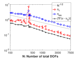
In the adaptive mesh refinement (AMR) procedure, we start with a initial mesh. The marking percent is set to be , i.e., the ordered elements (from the one with largest error indicator) that accounts for the first of the total error estimator get refined. With the stopping criteria that the total number of degree of freedoms (DOFs) be not greater than , the final meshes generated by and are provided in Fig. 2(a) and Fig. 2(b).
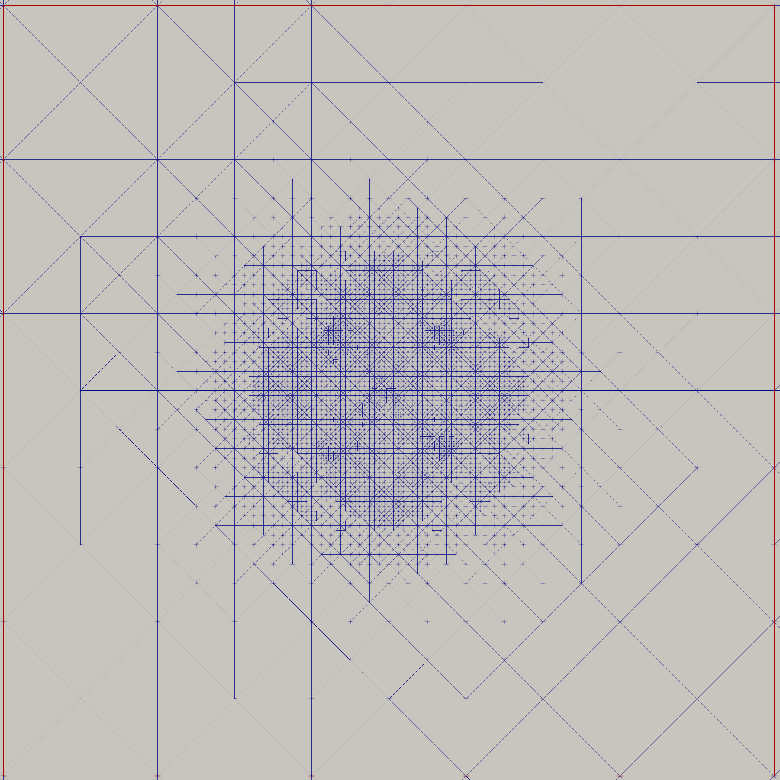 |
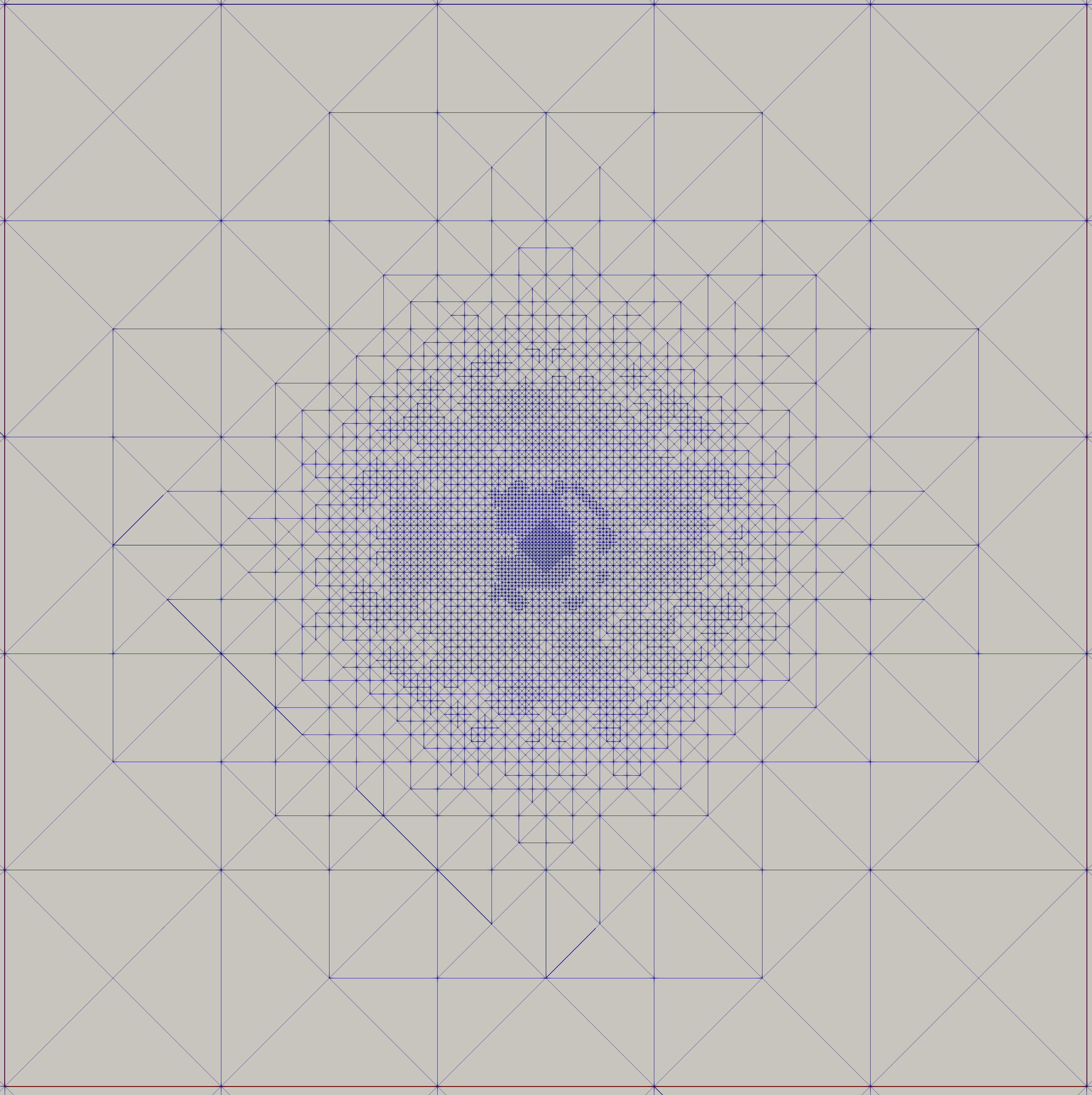 |
|
| (a)mesh by | (b)mesh by | |
 |
 |
 |
| (c)Errors by | (d)Errors by | (e)On uniform meshes |
From Fig. 2(c) and Fig. 2(d), we observe optimal convergence rates for both estimators. However, the efficiency index, which is defined by , of is more accurate with mean values and for Fig. 2(c) and Fig. 2(d), respectively, comparing to that of with mean values and for Fig. 2(c) and Fig. 2(d), respectively.
Example 5.2.
In this example, we test the Franke function [27] on the unit square domain,
This function has two peaks at and and one sink at . Since the boundary of the domain is regular, the purpose of this example is again to test the efficacy of our algorithm for Nitsche’s method on regular domain. However, the solution on the boundary is more volatile than in Example 5.1 and our numerical results show that this boundary volatility potentially causes extra challenges for the efficiency of Nitsche’s method that imposes the Dirichlet boundary condition weakly.
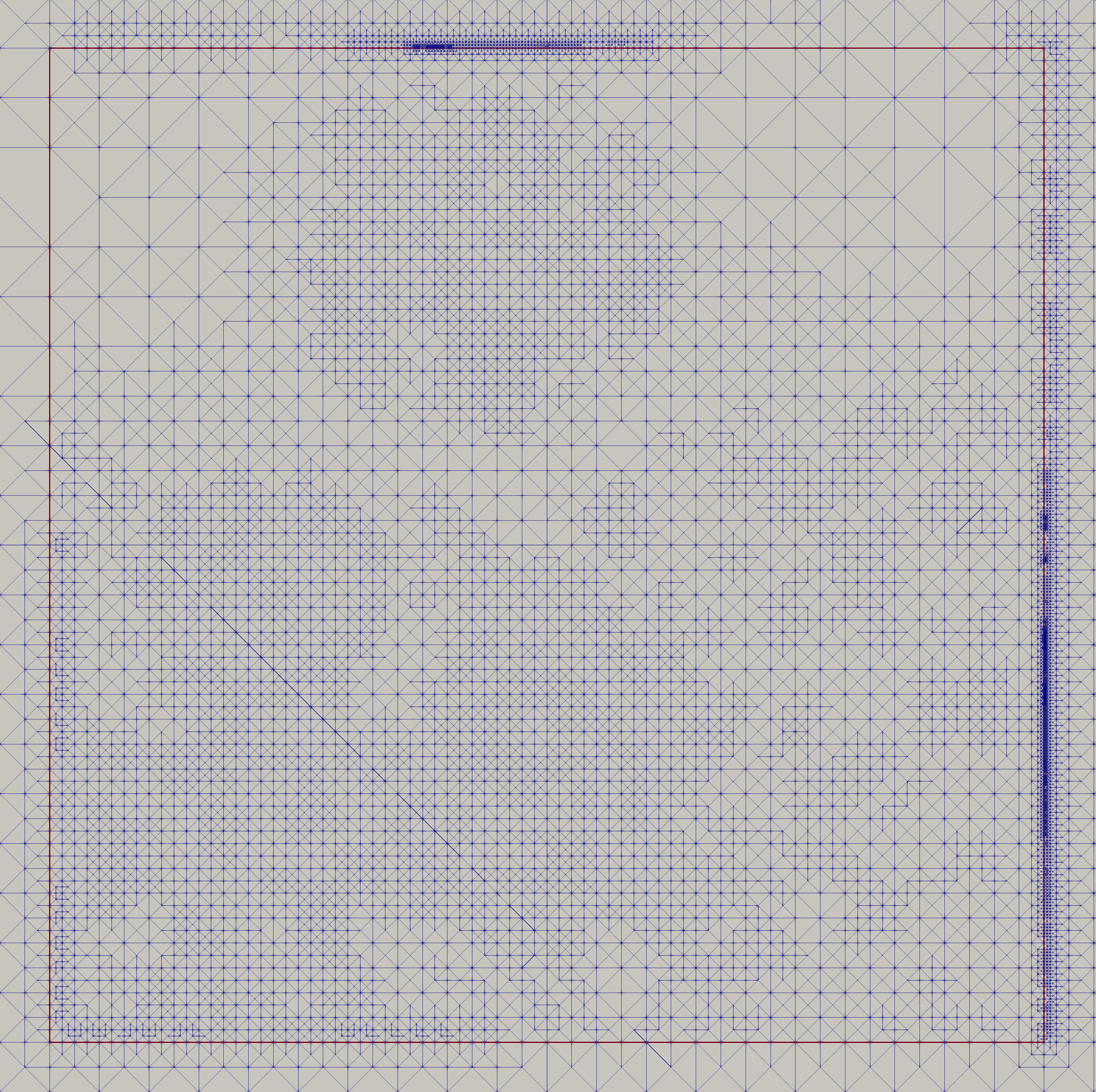
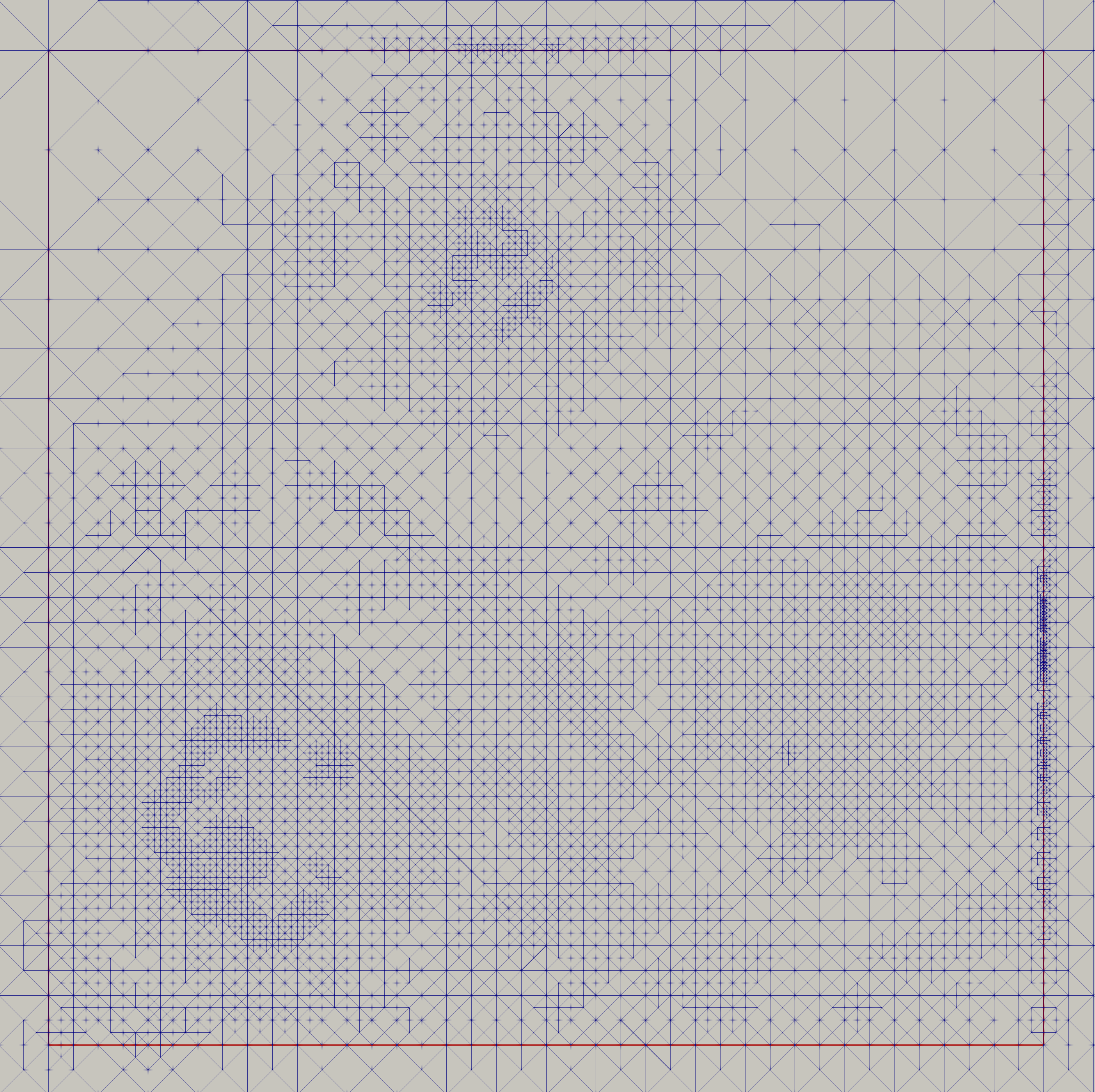
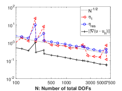
The optimal convergence results on uniform meshes for the errors and are verified in Fig. 3(e). With the same initial mesh and marking strategy as in Example 5.1, and with the stopping criteria that the total number of DOFs be not greater than , the final meshes generated using and are provided respectively in Fig. 3(a) and (b). Both meshes are similar with DOFs centered around the peaks and sinks. Since the solution is more volatile on some parts of the boundary, we also observe dense refinements on some right and upper parts of the boundary. However, the mesh in Fig. 3(a) puts relatively more DOFs on the boundary comparing to Fig. 3(b) on the boundary.
From Fig. 3(c) and Fig. 3(d), we observe optimal convergence for both the true error and the estimators in the overall pattern, however, with occasional oscillations, for both cases. Such oscillation is uniquely caused by the Nitsche method since it imposes the Dirichlet boundary condition weakly. Again, we observe that is more accurate than for most regular (non-oscillating) iterations. Nevertheless, it seems that has a stronger magnifying effect for the oscillation.
 |
 |
|
| (a)Mesh by | (b)Mesh by | |
 |
 |
 |
| (c)Errors by | (d)Errors by | (e)On uniform meshes |
Example 5.3.
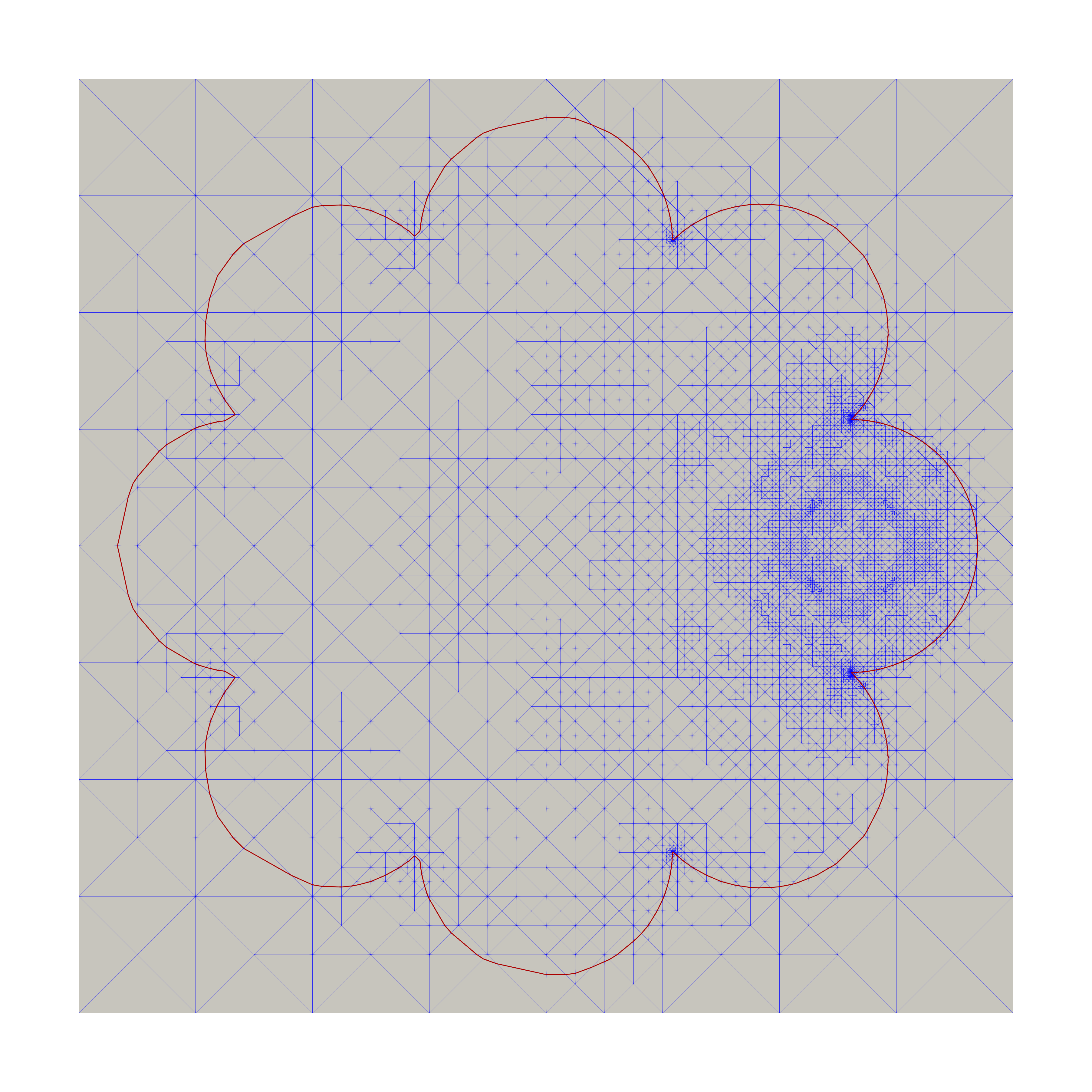
In this example, we test our algorithm on an irregular domain. The level set of the problem has a flower shape (see e.g., Fig. 4(a)) that has the following representation:
with
for , and
The domain boundary is defined to be the zero level set, i.e., . The data are given such that on and
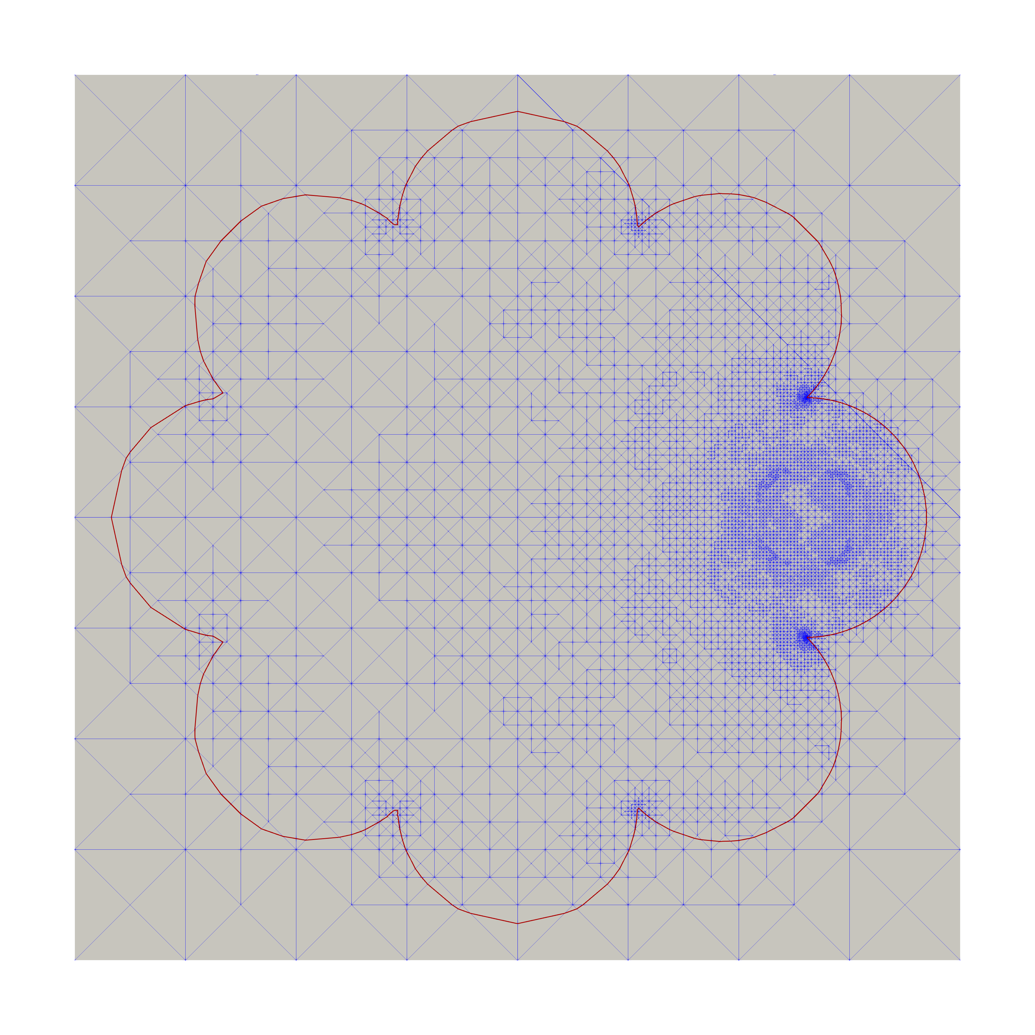
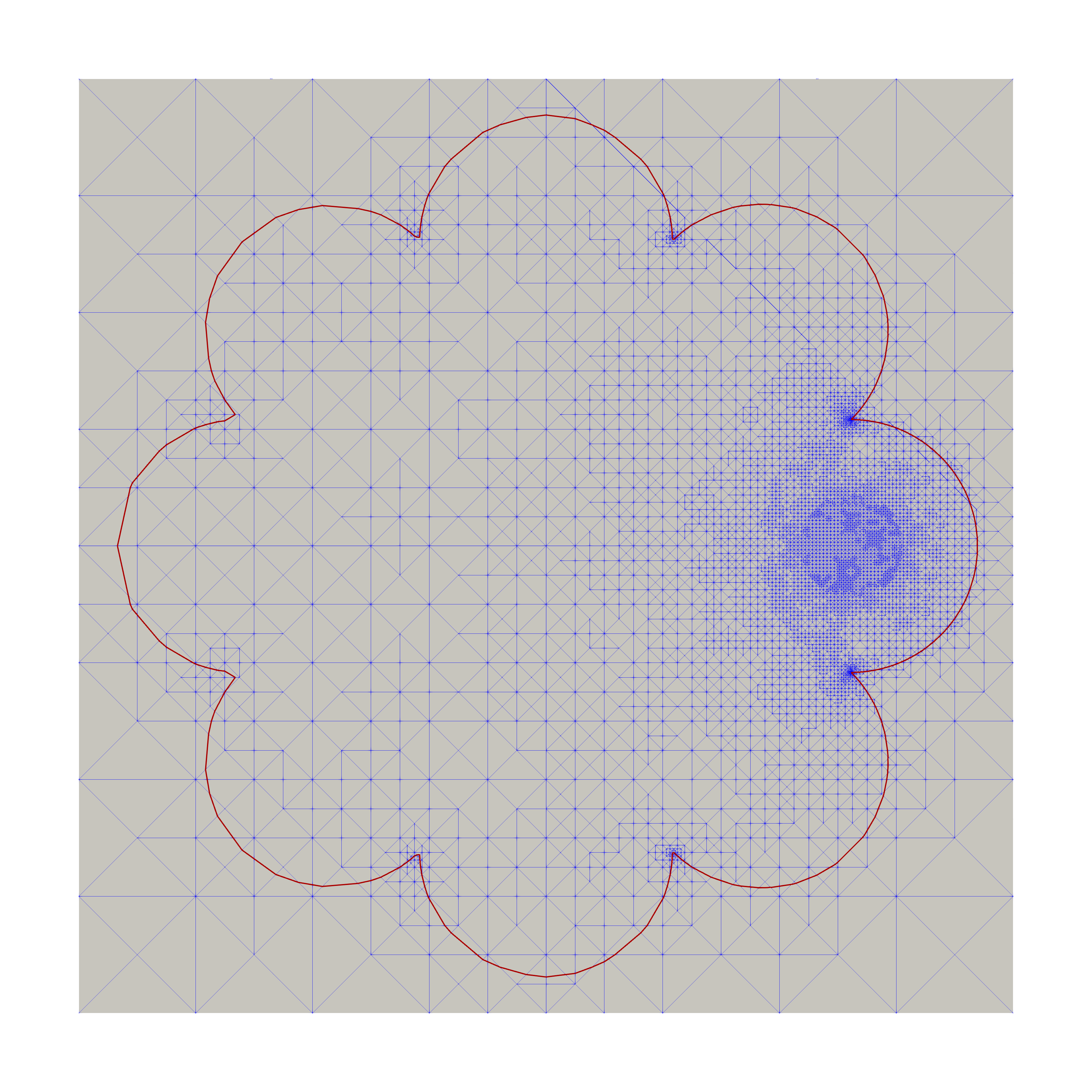
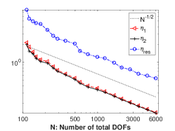
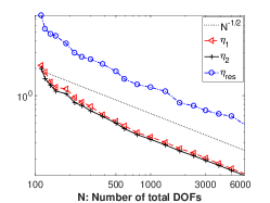
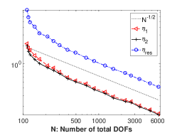
In the numerical scheme, we take and is approximated by its projection into the discontinuous piecewise constant space. We start with a crossed mesh on the rectangular domain . With the stopping criteria that the total number of DOFs be not greater than and marking percent set to be , the final meshes obtained by , and are given in Fig. 4(a), (b) and (c), respectively. We observe similar meshes for the three cases and DOFs are centered around the heat source. From Fig. 4(c), (d) and (e), we observe optimal convergence rate for all error estimators. In this example, is very close to since there are no dense refinement on the boundary, and is relatively bigger.
 |
 |
 |
| (a)Meshes by | (b)Meshes by | (c)Meshes by |
 |
 |
 |
| (d)Errors by | (e)Errors by | (f)Errors by |
Example 5.4.
In this example, we consider the reentrant problem whose solution has the following polar representation:
with and being the angle of the reentrant corner. In this example, we take . The domain is set to be , where is the ball with center and radius . It is easy to check that in .
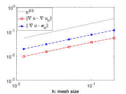
In the numerical scheme, we extend outside of by and take to be the conforming linear interpolation of with respect to . The optimal convergence results on uniform meshes for the errors and are verified in Fig. 5(e).
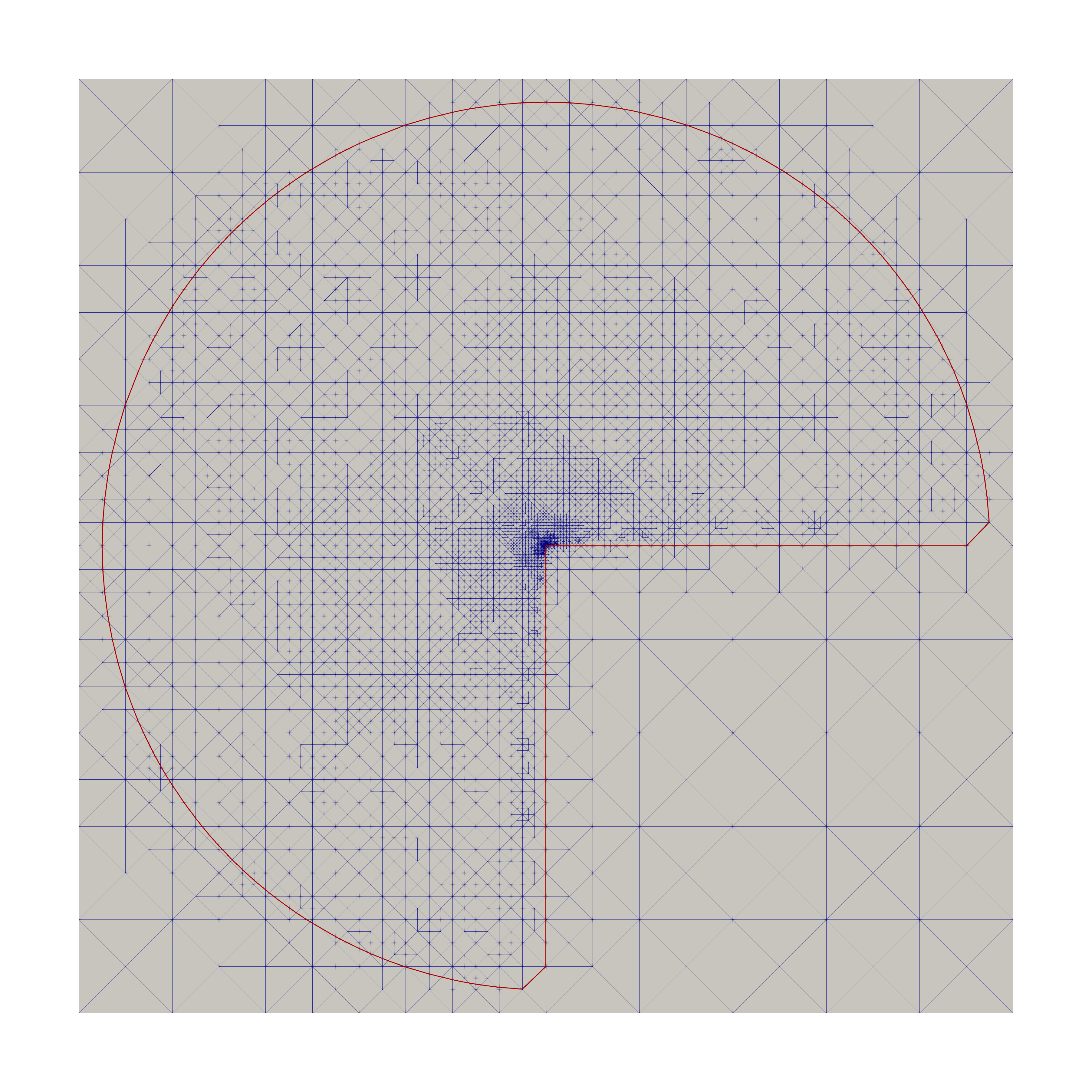
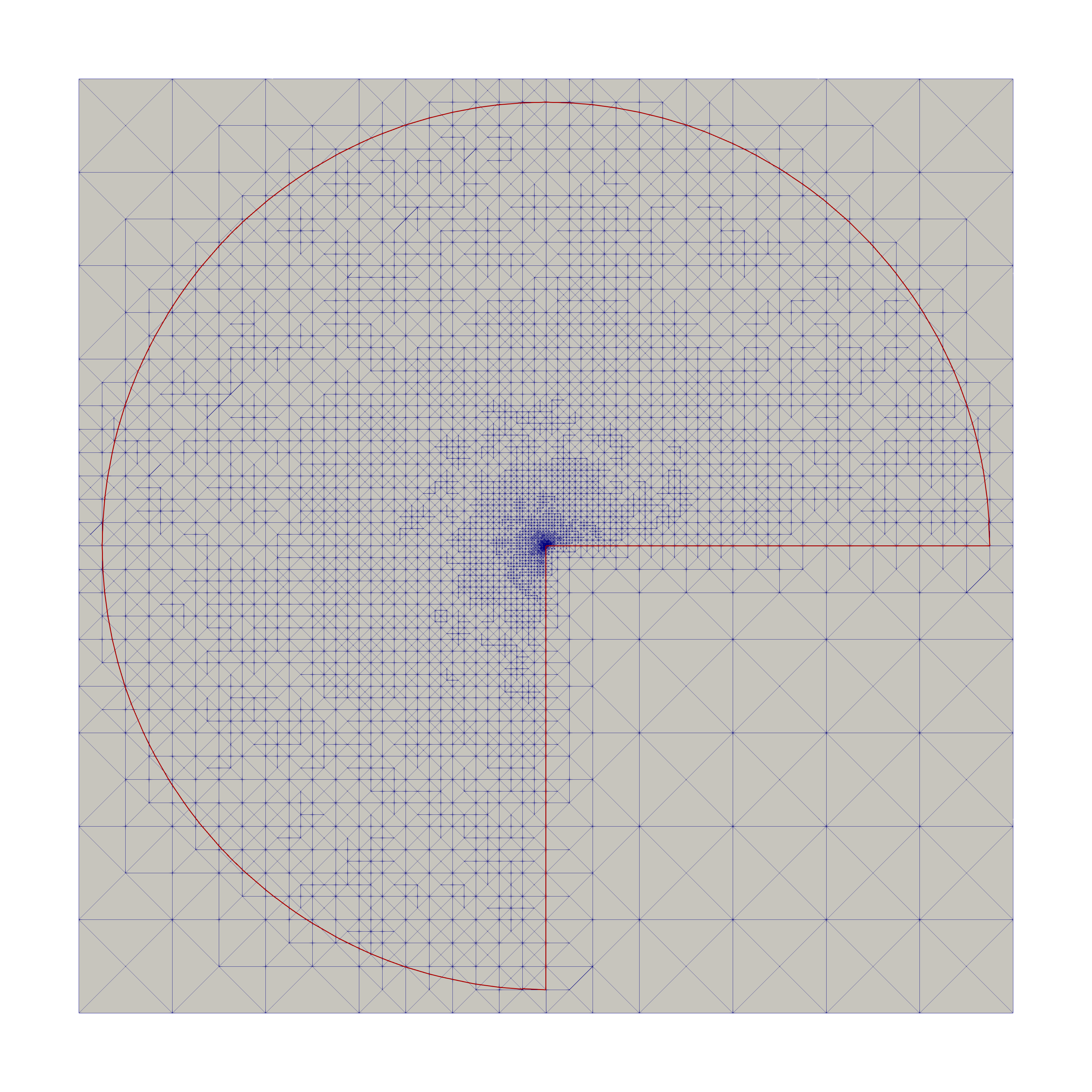
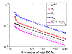
In the AMR procedure, we choose to use the initial mesh on the regular domain . With the marking percent set to be and the stopping criteria set such that the maximal number of degrees of freedom does not exceed , the final meshes generated by and are given in Fig. 5(a) and Fig. 5(b). The corresponding convergence rate of the estimators are presented in Fig. 5(c) and Fig. 5(d). We again observe optimal convergence for both AMR procedures. This again indicates that the estimators work equivalently effective for problems with reentrant singularity on the boundary. However, is more accurate than . For Fig. 5(c), the mean ratio for is , whereas the mean ratio for and is and , respectively. The corresponding ratios for Fig. 5(d) are similar. We note that for this example, using generates almost the same mesh as . However, is more accurate than in both cases.
 |
 |
|
| (a)Mesh by | (b)Mesh by | |
 |
 |
 |
| (c)Errors by | (d)Errors by | (e)Errors on uniform meshes |
References
- [1] M. Ainsworth, A posteriori error estimation for discontinuous Galerkin finite element approximation, SIAM Journal on Numerical Analysis, 45 (2007), pp. 1777–1798.
- [2] M. Ainsworth and R. Rankin, Fully computable bounds for the error in nonconforming finite element approximations of arbitrary order on triangular elements, SIAM Journal on Numerical Analysis, 46 (2008), pp. 3207–3232.
- [3] M. Ainsworth and O. J. Tinsley, A posteriori error estimation in finite element analysis, vol. 37, John Wiley & Sons, 2011.
- [4] S. Badia, F. Verdugo, and A. F. Martín, The aggregated unfitted finite element method for elliptic problems, Comput. Methods Appl. Mech. Engrg., 336 (2018), pp. 533–553, https://doi.org/10.1016/j.cma.2018.03.022, https://doi.org/10.1016/j.cma.2018.03.022.
- [5] J. W. Barrett and C. M. Elliott, A finite-element method for solving elliptic equations with Neumann data on a curved boundary using unfitted meshes, IMA J. Numer. Anal., 4 (1984), pp. 309–325, https://doi.org/10.1093/imanum/4.3.309.
- [6] P. Bastian and B. Rivière, Superconvergence and projection for discontinuous Galerkin methods, International journal for numerical methods in fluids, 42 (2003), pp. 1043–1057.
- [7] R. Becker, D. Capatina, and R. Luce, Local flux reconstructions for standard finite element methods on triangular meshes, SIAM Journal on Numerical Analysis, 54 (2016), pp. 2684–2706.
- [8] S. Bertoluzza, M. Ismail, and B. Maury, The fat boundary method: semi-discrete scheme and some numerical experiments, in Domain Decomposition Methods in Science and Engineering, vol. 40 of Lect. Notes Comput. Sci. Eng., Springer, Berlin, 2005, pp. 513–520, https://doi.org/10.1007/3-540-26825-1_53.
- [9] D. Boffi, F. Brezzi, M. Fortin, et al., Mixed finite element methods and applications, vol. 44, Springer, 2013.
- [10] D. Braess, T. Fraunholz, and R. H. Hoppe, An equilibrated a posteriori error estimator for the interior penalty discontinuous Galerkin method, SIAM Journal on Numerical Analysis, 52 (2014), pp. 2121–2136.
- [11] D. Braess, V. Pillwein, and J. Schöberl, Equilibrated residual error estimates are p-robust, Computer Methods in Applied Mechanics and Engineering, 198 (2009), pp. 1189–1197.
- [12] E. Burman, Ghost penalty, C. R. Math. Acad. Sci. Paris, 348 (2010), pp. 1217–1220, https://doi.org/10.1016/j.crma.2010.10.006.
- [13] E. Burman and A. Ern, An unfitted hybrid high-order method for elliptic interface problems, SIAM J. Numer. Anal., 56 (2018), pp. 1525–1546, https://doi.org/10.1137/17M1154266.
- [14] E. Burman and P. Hansbo, Fictitious domain finite element methods using cut elements: I. A stabilized Lagrange multiplier method, Comput. Methods Appl. Mech. Engrg., 199 (2010), pp. 2680–2686, https://doi.org/10.1016/j.cma.2010.05.011.
- [15] E. Burman and P. Hansbo, Fictitious domain finite element methods using cut elements: II. A stabilized Nitsche method, Appl. Numer. Math., 62 (2012), pp. 328–341, https://doi.org/10.1016/j.apnum.2011.01.008.
- [16] E. Burman, P. Hansbo, and M. G. Larson, A cut finite element method with boundary value correction, Math. Comp., 87 (2018), pp. 633–657, https://doi.org/10.1090/mcom/3240.
- [17] E. Burman, C. He, and M. G. Larson, A posteriori error estimates with boundary correction for a cut finite element method, IMA Journal of Numerical Analysis, (2020), https://doi.org/https://doi.org/10.1093/imanum/draa085.
- [18] Z. Cai, C. He, and S. Zhang, Residual-based a posteriori error estimate for interface problems: nonconforming linear elements, Mathematics of Computation, 86 (2017), pp. 617–636, https://doi.org/10.1090/mcom/3151.
- [19] Z. Cai, C. He, and S. Zhang, Generalized Prager-Synge inequality and equilibrated error estimators for discontinuous elements, arXiv preprint arXiv:2001.09102, (2020).
- [20] Z. Cai and S. Zhang, Robust equilibrated residual error estimator for diffusion problems: conforming elements, SIAM Journal on Numerical Analysis, 50 (2012), pp. 151–170.
- [21] D. A. Di Pietro and A. Ern, Mathematical aspects of discontinuous Galerkin methods, vol. 69 of Mathématiques & Applications (Berlin) [Mathematics & Applications], Springer, Heidelberg, 2012, https://doi.org/10.1007/978-3-642-22980-0.
- [22] P. Di Stolfo, A. Rademacher, and A. Schröder, Dual weighted residual error estimation for the finite cell method, Journal of Numerical Mathematics, 27 (2019), pp. 101–122.
- [23] W. Dörfler, A convergent adaptive algorithm for Poisson’s equation, SIAM Journal on Numerical Analysis, 33 (1996), pp. 1106–1124.
- [24] A. Ern, S. Nicaise, and M. Vohralík, An accurate flux reconstruction for discontinuous Galerkin approximations of elliptic problems, Comptes Rendus Mathematique, 345 (2007), pp. 709–712.
- [25] A. Ern and M. Vohralík, Polynomial-degree-robust a posteriori estimates in a unified setting for conforming, nonconforming, discontinuous Galerkin, and mixed discretizations, SIAM Journal on Numerical Analysis, 53 (2015), pp. 1058–1081.
- [26] D. Estep, M. Pernice, S. Tavener, and H. Wang, A posteriori error analysis for a cut cell finite volume method, Computer methods in applied mechanics and engineering, 200 (2011), pp. 2768–2781.
- [27] R. Franke, A critical comparison of some methods for interpolation of scattered data, tech. report, Navel Postgraduate School Monterey CA, 1979.
- [28] R. Glowinski and T.-W. Pan, Error estimates for fictitious domain/penalty/finite element methods, Calcolo, 29 (1992), pp. 125–141 (1993), https://doi.org/10.1007/BF02576766.
- [29] P. Grisvard, Elliptic problems in nonsmooth domains, vol. 69 of Classics in Applied Mathematics, Society for Industrial and Applied Mathematics (SIAM), Philadelphia, PA, 2011, https://doi.org/10.1137/1.9781611972030.ch1. Reprint of the 1985 original [ MR0775683], With a foreword by Susanne C. Brenner.
- [30] A. Hansbo and P. Hansbo, An unfitted finite element method, based on Nitsche’s method, for elliptic interface problems, Comput. Methods Appl. Mech. Engrg., 191 (2002), pp. 5537–5552, https://doi.org/10.1016/S0045-7825(02)00524-8.
- [31] J. Haslinger and Y. Renard, A new fictitious domain approach inspired by the extended finite element method, SIAM J. Numer. Anal., 47 (2009), pp. 1474–1499, https://doi.org/10.1137/070704435.
- [32] P. Huang, H. Wu, and Y. Xiao, An unfitted interface penalty finite element method for elliptic interface problems, Comput. Methods Appl. Mech. Engrg., 323 (2017), pp. 439–460, https://doi.org/10.1016/j.cma.2017.06.004, https://doi.org/10.1016/j.cma.2017.06.004.
- [33] A. Johansson and M. G. Larson, A high order discontinuous Galerkin Nitsche method for elliptic problems with fictitious boundary, Numer. Math., 123 (2013), pp. 607–628, https://doi.org/10.1007/s00211-012-0497-1, https://doi.org/10.1007/s00211-012-0497-1.
- [34] K.-Y. Kim, Flux reconstruction for the p2 nonconforming finite element method with application to a posteriori error estimation, Applied Numerical Mathematics, 62 (2012), pp. 1701–1717.
- [35] L. D. Marini, An inexpensive method for the evaluation of the solution of the lowest order Raviart–Thomas mixed method, SIAM journal on numerical analysis, 22 (1985), pp. 493–496.
- [36] A. Massing, M. G. Larson, A. Logg, and M. E. Rognes, A stabilized Nitsche fictitious domain method for the Stokes problem, J. Sci. Comput., 61 (2014), pp. 604–628, https://doi.org/10.1007/s10915-014-9838-9.
- [37] J. Nitsche, Über ein Variationsprinzip zur Lösung von Dirichlet-Problemen bei Verwendung von Teilräumen, die keinen Randbedingungen unterworfen sind, Abh. Math. Sem. Univ. Hamburg, 36 (1971), pp. 9–15, https://doi.org/10.1007/BF02995904. Collection of articles dedicated to Lothar Collatz on his sixtieth birthday.
- [38] L. H. Odsæter, M. F. Wheeler, T. Kvamsdal, and M. G. Larson, Postprocessing of non-conservative flux for compatibility with transport in heterogeneous media, Computer Methods in Applied Mechanics and Engineering, 315 (2017), pp. 799–830.
- [39] H. Sun, D. Schillinger, and S. Yuan, Implicit a posteriori error estimation in cut finite elements, Computational Mechanics, 65 (2020), pp. 967–988.
- [40] R. Verfürth, A posteriori error estimation and adaptive mesh-refinement techniques, Journal of Computational and Applied Mathematics, 50 (1994), pp. 67–83, https://doi.org/10.1016/0377-0427(94)90290-9.