Extended reduced-order surrogate models for scalar-tensor gravity in the strong field and applications to binary pulsars and gravitational waves

Abstract

Statistically sound tests of scalar-tensor gravity theories in the strong-field regime usually involves computationally intensive calculations. In this study, we construct a reduced order surrogate model for the scalar-tensor gravity of Damour and Esposito-Farèse (DEF) with spontaneous scalarization phenomena developed for neutron stars (NSs). This model allows us to perform a rapid and comprehensive prediction of NS properties, including mass, radius, moment of inertia, effective scalar coupling, and two extra coupling parameters. We code the model in the pySTGROMX package, as an extension of our previous work, that speeds up the calculations at two and even three orders of magnitude and yet still keeps accuracy of $\sim 1\%$. Using the model, we can calculate all the post-Keplerian parameters in the timing of binary pulsars conveniently, which provides a quick approach for us to place comprehensive constraints on the DEF theory. We perform Markov-chain Monte Carlo simulations with the model to constrain the parameters of the DEF theory with well-timed binary pulsars. Utilizing five NS-white dwarf and three NS-NS binaries, we obtain the most stringent constraints on the DEF theory up to now. Our work provides a public tool for quick evaluation of NSs’ derived parameters to test gravity in the strong-field regime.

I Introduction

Albert Einstein’s theory of general relativity (GR) Einstein (1915) remains the most accurate theory of gravity for more than a century. This elegant theory has passed all tests with flying colors from, e.g., the Solar System experiments Will (2014), cosmological observation Clifton et al. (2012), the timing of binary pulsars Stairs (2003); Wex (2014); Shao and Wex (2016), and gravitational waves (GWs) from coalescing binary black holes (BBHs) Abbott et al. (2016, 2017a, 2019a, 2021a) and binary neutron stars (BNSs) Abbott et al. (2017b, c, 2019b). From the Earth up to the Universe, from weak to strong gravitational field, GR remains the gold standard.

There are good theoretical reasons to go beyond GR, however Berti et al. (2015). Therefore, even with the success of GR, considerable efforts are still being made for alternative theories of gravity (see Refs. Will (2014, 2018) for a review). In GR, gravity is mediated solely by a massless, spin-2 tensor field, namely the metric of spacetime $g_{\mu\nu}$. Differently from GR, scalar-tensor theories of gravity, as natural and well-motivated alternatives, add one or more extra scalar degrees of freedom in the gravitational sector. They not only arise naturally as a possible low-energy limit of higher dimensional theories, such as Kaluza-Klein theory Kaluza (2018); Klein (1926) and string theories Fujii and Maeda (2007), but also have a potential connection to the inflation, the dark energy, and a yet unknown unified theory of quantum gravity Clifton et al. (2012). Originally suggested by Scherrer in 1941 Goenner (2012), the most popular scalar-tensor gravity theories are developed in a modern framework by Jordan Jordan (1949, 1959), Fierz Fierz (1956), Brans and Dicke Brans and Dicke (1961) (JFBD; see a review in Ref. Fujii and Maeda (2007)). JFBD-like theories, as metric theories of gravity, do not violate the weak equivalence principle but the strong equivalence principle (SEP) due to the nonminimally coupled scalar field in the Einstein-Hilbert action Shao and Wex (2016); Will (2018). Tests of SEP, which is the heart of GR, provide a powerful tool to experimentally constrain these theories.

In this paper, we restrict our attention to a category of JFBD-like theory proposed by Damour and Esposito-Farèse (DEF) Damour and Esposito-Farèse (1992, 1993, 1996), where prominent violations of the SEP due to nonperturbative strong-field effects are known to arise. The DEF theory can pass present weak-field gravitational tests, such as the Cassini experiment Bertotti et al. (2003), but still exhibits very significant strong-field deviations away from GR in the systems involving strongly self-gravitating neutron stars (NSs) Damour and Esposito-Farèse (1993); Shao et al. (2017).

In the weak-field regime, observations in the Solar System, such as the Cassini probe Bertotti et al. (2003), have placed stringent bounds on scalar-tensor theories. Shapiro time-delay measurements with the Cassini spacecraft have confirmed to a high precision $\sim 10^{-5}$ that the Eddington-Robertson-Schiff parameters are in agreement with GR prediction in the parametrized post-Newtonian (PPN) framework Will (2018). Nevertheless, the DEF theory is compatible with the weak-field tests as long as its weak-field coupling parameter, $\alpha_{0}$, is small.

However, in the strong-field regime for the DEF theory, even with a small $\alpha_{0}$, one kind of nonperturbative strong-field effects, the so-called spontaneous scalarization, occurs as a scalar analogue of the phase transition in ferromagnetism Damour and Esposito-Farèse (1993, 1996); Sennett et al. (2017). It naturally arises in an isolated compact star such as a NS under a certain condition with the scalar field excited far above its background value. Such deviation from GR introduces considerable modifications into the properties of scalarized compact stars. It also affects the relativistic orbital motion if a scalarized NS is in a binary, via, e.g., a body-dependent effective gravitational constant, extra gravitational binding energy related to the scalar field, and dipolar radiation in addition to the canonical quadrupolar radiation in GR Damour and Esposito-Farèse (1992); Damour (2009). Long-term monitoring of binary pulsars and transient observations of GWs from BNS coalescences are therefore powerful tools to probe the contribution from spontaneous scalarization in extreme environments of strong gravitational fields Wex (2014); Damour and Esposito-Farèse (1996); Anderson et al. (2019).

The high-precision timing of binary pulsars provides some of the tightest gravity tests with strongly self-gravitating bodies in the quasi-stationary strong-field gravity regime Stairs (2003); Wex (2014); Shao and Wex (2016); Shao (2019a). In this regime, gravitational fields are strong with large spacetime curvature in the vicinity of the NSs while the typical velocity $v$ is much smaller than the speed of light $c$ with a ratio of $v/c\sim 10^{-3}$. To extract the information from pulsar timing for testing gravity theories, the parametrized post-Keplerian (PPK) formalism was constructed as a general framework Damour and Taylor (1992). The dynamical information can be obtained from the pulsar timing and pulse-structure data by fitting the data to a model consisting of the theory-independent Keplerian and post-Keplerian parameters.

In the DEF theory, one of the PPK parameters, $\dot{P}_{b}$, which is related to binary orbital decay, is modified due to the extra dipolar radiation Damour and Esposito-Farèse (1992). The dipolar contribution, corresponding to a $-1$ post-Newtonian (PN) correction, may dominate the radiation when $v/c$ is small. Thus, at the early time of the binary system, due to a small $v/c\sim 10^{-3}$, this mechanism enhances the energy flux of GWs emitted from the system and thus changes $\dot{P}_{b}$ in a noticeable way. In addition, the DEF theory predicts that, due to the spontaneous scalarization, all the PPK parameters are modified from the GR prediction Damour and Taylor (1992). Therefore, these parameters can be combined to constrain the DEF theory Damour and Esposito-Farèse (1996).

With the detection of GW events, especially coalescing BNSs, GW170817 Abbott et al. (2017b) and a possible candidate GW190425 Abbott et al. (2021b) up to date, we have a new testbed in probing the strong-field gravity in highly dynamical regime. Matched-filter analyses, used in parameter estimation of GWs Finn (1992), are sensitive to GW phase evolution, which is modified in the DEF theory and can be distinguished from GR. Thus, GW signals can also be utilized to bound the DEF theory.

So far, however, the bound on dipolar radiation from GW of coalescing BNSs is still looser than that from the timing of binary pulsars Shao et al. (2017); Zhao et al. (2019), since dipolar radiation corresponds to a $-1$ PN correction and plays a relatively important role when $v/c\ll 1$, corresponding to low-frequency signals, where sensitivity of the LIGO/Virgo detectors is limited. Future ground-based and space-based GW detectors with a better low-frequency sensitivity, such as Cosmic Explorer (CE) Abbott et al. (2017d), Einstein Telescope (ET) Hild et al. (2011), DECi-hertz Interferometer Gravitational wave Observatory (DECIGO) Yagi and Tanaka (2010) and Decihertz Observatory (DO) Sedda et al. (2020); Arca Sedda et al. (2021) will place tighter constraints on gravity theories by either enabling observations below $10\,{\rm Hz}$ or increasing the sensitivity further (see e.g. Ref. Liu et al. (2020a)).

To perform tests on the scalar-tensor gravity, first, one must derive the relevant predictions on observations precisely. The predictions on some properties of a NS, such as its radius $R$, mass $m_{A}$, moment of inertia $I_{A}$, and the scalar coupling parameter $\alpha_{A}$, are derived by numerically integrating the modified Tolman-Oppenheimer-Volkoff (mTOV) equations of a slowly rotating NS with the shooting method Damour and Esposito-Farèse (1993, 1996). This integration depends on the equation of state (EOS) of NS matters, which is, unfortunately, still full of large uncertainties (see e.g. Refs. Lattimer and Prakash (2001); Shao (2019b)).

Apart from the NSs’ properties above, some other properties in the DEF theory are also required to predict some of PPK parameters in binary pulsars. They consist of the coupling parameters $\beta_{A}$ and $k_{A}$, which are derived by calculating the derivatives of scalar coupling $\alpha_{A}$ and moment of inertia $I_{A}$, with respect to the scalar field at infinity Damour and Esposito-Farèse (1996). Note that the calculations of $\beta_{A}$ and $k_{A}$ should be performed for a fixed value of baryonic mass $\bar{m}_{A}$. This procedure requires one to perform the shooting method for both $\bar{m}_{A}$ and the scalar field simultaneously Damour and Esposito-Farèse (1996). The calculations for such parameters are very time-consuming and thus expensive for large-scale computation.

In practice, to constrain the free parameters in the DEF theory in a statistically sound way, we use Bayesian inference through Markov-chain Monte Carlo (MCMC) simulations. This approach involves the evaluation of the likelihood function hundreds of thousands to millions of times with solving the mTOV equations each time. The whole simulation is thus time-consuming and expensive. Such computationally intensive studies have been conducted in Ref. Shao et al. (2017) for the first time.

In this study, we avoid solving the mTOV equations iteratively and repeatedly by trial and error during the data analysis process. Instead, we build a reduced order surrogate model (ROM) in advance with the existing mTOV solutions. The surrogate model reduces the dimensions of the existing mTOV solutions and yet still keeps high accuracy. This model is therefore very efficient by a linear algebraic operation rather than the iterative integration. The ROM-related techniques have been widely applied in GW science (see Ref. Tiglio and Villanueva (2021) for a review), e.g., fast evaluation of GW waveforms Field et al. (2014) and acceleration of GW parameter estimation Canizares et al. (2013, 2015). Following the earlier work of Zhao et al. (2019), we extend our model to predict all the PPK parameters, not just the orbital period decay parameter $\dot{P}_{b}$. To explore EOS-dependent aspects, in this work, we choose 15 EOSs that are all consistent with the maximum mass of NSs being larger than $2\,\mathrm{M_{\odot}}$. This extends the number of EOSs in Ref. Zhao et al. (2019). We use the central matter density $\rho_{c}$ of a NS to predict its radius $R$, mass $m_{A}$, moment of inertia $I_{A}$ and its derivative $k_{A}$, as well as the effective scalar coupling $\alpha_{A}$ and its derivative $\beta_{A}$. Our models keep $\sim 1\%$ level of accuracy. According to our performance tests, one can speed up the calculations by at least two and even three orders of magnitude for the coupling parameters $\beta_{A}$ and $k_{A}$, and yet still keep the due accuracy. We demonstrate various applications with binary pulsars to illustrate the practical value of our ROMs.

The improvements of this work include the followings.

1. We use a larger set of EOSs.

2. We calculate the mTOV equation to build ROMs in the DEF theory for slowly rotating NSs, instead of the nonrotating ones, to predict the moment of inertia and its derivative.

3. We extend our ROMs to the coupling parameters by calculating the derivatives of $\alpha_{A}$ and $I_{A}$, and thus we can predict all the PPK parameters with new ROMs.

4. Our ROMs speed up the calculation by two to even three orders of magnitude.

5. We utilize the binary pulsars including double NSs to derive tight constraints on the DEF theory.

The rest of this paper is organized as follows. Section II briefly reviews the nonperturbative spontaneous-scalarization phenomena for slowly rotating NSs and discusses the modifications of PPK parameters, including orbital period decay, periastron advance rate, and Einstein delay parameter in the DEF gravity . In Sec. III, we present the method of solving the mTOV equations, calculating the derived parameters, and constructing the ROMs for large-scale calculations. We code the model in the pySTGROMX (a.k.a. pySTGROM eXtension) package which is public for easy use for the community. In Sec. IV, with pySTGROMX, we perform accelerated MCMC simulation and constrain the DEF theory tightly by combining the relevant PPK parameters available from observations of five NS-white dwarf (WD) systems and three NS-NS systems. We summarize our conclusions in Sec. V.

II Spontaneous scalarization in the DEF Theory

The DEF theory is defined by the following general action in the Einstein frame Damour and Esposito-Farèse (1993, 1996),

$$S= \frac{c^{4}}{16\pi G_{\star}}\int\frac{\differential^{4}x}{c}\sqrt{-g_{\star}}\left[R_{\star}-2g^{\mu\nu}_{\star}\partial_{\mu}\varphi\partial_{\nu}\varphi-V(\varphi)\right]$$ (1)

$$+S_{m}\left[\psi_{m};A^{2}(\varphi)g^{\star}_{\mu\nu}\right]\,.$$

Here, $G_{\star}$ denotes the bare gravitational constant, $g_{\star}\equiv{\rm det}\,g^{\star}_{\mu\nu}$ is the determinant of “Einstein metric” $g^{\star}_{\mu\nu}$, $R_{\star}$ is the Ricci curvature scalar of $g^{\star}_{\mu\nu}$, and $\varphi$ is a dynamical scalar field. In the matter part $S_{m}$ of Eq. (1), $\psi_{m}$ denotes matter fields collectively, and it couples to $\varphi$ by the conformal coupling factor $A(\varphi)$. In this study, we assume that the potential, $V(\varphi)$, is a slowly varying function at the typical scale of the system we consider and set $V(\varphi)=0$ in our calculation for simplicity (see Refs. Ramazanoğlu and Pretorius (2016); Xu et al. (2020) for a massive scalar field).

Varying the action (1) yields the field equations,

$$R^{\star}_{\mu\nu} = \partial_{\mu}\varphi\partial_{\nu}\varphi+\frac{8\pi G_{\star}}{c^{4}}\left(T^{\star}_{\mu\nu}-\frac{1}{2}T^{\star}g^{\star}_{\mu\nu}\right)\,,$$ (2)

$$\Box_{g^{\star}}\varphi = -\frac{4\pi G_{\star}}{c^{4}}\alpha(\varphi)T_{\star}\,,$$ (3)

where the matter stress-energy tensor is

$$T^{\mu\nu}_{\star}\equiv\frac{2c}{\sqrt{-g_{\star}}}\left(\frac{\delta S_{m}}{\delta g^{\star}_{\mu\nu}}\right)\,,$$ (4)

and $T^{\star}\equiv g^{\star}_{\mu\nu}T^{\mu\nu}_{\star}$ is the trace. In Eq. (3), the parameter $\alpha(\varphi)$ is defined as the derivative of logarithmic $A(\varphi)$,

$$\alpha(\varphi)\equiv\frac{\partial\ln A(\varphi)}{\partial\varphi}\,,$$ (5)

which indicates the coupling strength between the scalar field and matters [see Eq. (3)].

In the DEF theory Damour and Esposito-Farèse (1996), $\ln A(\varphi)$ is designated as

$$\ln A(\varphi)=\frac{1}{2}\beta_{0}\varphi^{2}\,,$$ (6)

where

$$\beta_{0}\equiv\frac{\partial^{2}\ln A(\varphi)}{\partial\varphi^{2}}\Bigg{|}_{\varphi=\varphi_{0}}\,,$$ (7)

is a free parameter with $\varphi_{0}$ the asymptotic scalar field value of $\varphi$ at spatial infinity. Then $\alpha(\varphi)=\partial\ln A(\varphi)/\partial\varphi=\beta_{0}\varphi$, and we further denote $\alpha_{0}\equiv\beta_{0}\varphi_{0}$. Note that we have $\alpha_{0}=\beta_{0}=0$ in GR.

For NSs, nonperturbative scalarization phenomena develop when $\beta_{0}\lesssim-4$ Damour and Esposito-Farèse (1993); Barausse et al. (2013). Generally, a more negative $\beta_{0}$ means more manifest spontaneous scalarization in the strong-field regime. In such case, the effective scalar coupling for a NS “$A$” with a total mass-energy of $m_{A}$ is

$$\alpha_{A}\equiv\frac{\partial\ln m_{A}(\varphi)}{\partial\varphi}\Bigg{|}_{\varphi=\varphi_{0}}\,,$$ (8)

which measures the effective coupling strength between the scalar field and the NS.

Now we consider a scalarized NS in a binary system in the DEF theory. For a binary pulsar system with the pulsar labeled “$A$” and its companion labeled “$B$”, the parameters $\alpha_{A}$ and $\alpha_{B}$ contribute to the secular change of the orbital period Damour and Esposito-Farèse (1996). In this work, we investigate two contributions to $\dot{P}_{b}$, the dipolar contribution, $\dot{P}_{b}^{\mathrm{dipole}}$, and the quadrupolar contribution, $\dot{P}_{b}^{\mathrm{quad}}$. They are defined by Damour and Esposito-Farèse (1996)

$$\dot{P}_{b}^{\mathrm{dipole}} = -\frac{2\pi G_{\star}n_{b}}{c^{3}}g(e)\frac{m_{A}m_{B}}{m_{A}+m_{B}}\left(\alpha_{A}-\alpha_{B}\right)^{2}\,,$$ (9)

$$\dot{P}_{b}^{\mathrm{quad}} = -\frac{192\pi G_{AB}^{5/3}n_{b}^{5/3}}{5c^{5}(1+\alpha_{A}\alpha_{B})}f(e)\frac{m_{A}m_{B}}{(m_{A}+m_{B})^{1/3}}\,,$$ (10)

where $n_{b}\equiv 2\pi/P_{b}$, and

$$g(e)\equiv \left(1-e^{2}\right)^{-5/2}\left(1+\frac{e^{2}}{2}\right)\,,$$ (11)

$$f(e)\equiv \left(1-e^{2}\right)^{-7/2}\left(1+\frac{73}{24}e^{2}+\frac{37}{94}e^{4}\right)\,.$$ (12)

Here the bare gravitational constant in Eq. (9), $G_{\star}$, is obtained with the Newtonian constant $G_{N}$ by $G_{\star}=G_{N}/(1+\alpha_{0}^{2})$ Damour and Esposito-Farèse (1992), owing to the weak field coupling. The body-dependent effective gravitational constant in Eq. (10), $G_{AB}$, is given by $G_{AB}\equiv G_{\star}(1+\alpha_{A}\alpha_{B})$. The quadrupolar contribution $\dot{P}_{b}^{\mathrm{quad}}$ is close to the prediction of GR with a negligible correction, while the dipolar contribution $\dot{P}_{b}^{\mathrm{dipole}}$ is the dominant additional contribution in the DEF theory. Other subleading contributions induced by the scalar field can be neglected in this study [see Eq. (6.52) of Ref. Damour and Esposito-Farèse (1992)]. Note that the effective scalar coupling approaches to $\alpha_{0}$ for WDs in the weak field and becomes zero for BHs since the DEF theory still satisfies the no-hair theorem Abbott et al. (2017a); Berti et al. (2015). Thus, considering Eq. (9), the contribution of dipolar radiation to $\dot{P}_{b}$ plays an important role in NS-WD, NS-BH, and asymmetric NS-NS binaries. In those binaries, there could be a large difference between $\alpha_{A}$ and $\alpha_{B}$.

Similarly to $\alpha_{A}$, we define

$$\beta_{A}\equiv\frac{\partial\alpha_{A}}{\partial\varphi}\Bigg{|}_{\varphi=\varphi_{0}}\,,$$ (13)

which is the strong-field analogue of the parameter $\beta_{0}$. Then the theoretical prediction for the periastron advance rate in the DEF theory is Damour and Esposito-Farèse (1996)

$$\dot{\omega}^{\rm th}(m_{A},m_{B}) \equiv \frac{3n_{b}}{1-e^{2}}\left(\frac{G_{AB}(m_{A}+m_{B})n_{b}}{c^{3}}\right)^{2/3}$$

$$\times\left[\frac{1-\frac{1}{3}\alpha_{A}\alpha_{B}}{1+\alpha_{A}\alpha_{B}}-\frac{X_{A}\beta_{B}\alpha^{2}_{A}+X_{B}\beta_{A}\alpha^{2}_{B}}{6(1+\alpha_{A}\alpha_{B})^{2}}\right]\,,$$

where $X_{A}\equiv m_{A}/(m_{A}+m_{B})\equiv 1-X_{B}$. Finally, we consider a slowly-rotating NS with moment of inertia (in Einstein units) $I_{A}$. We denote

$$k_{A}\equiv-\frac{\partial\ln I_{A}}{\partial\varphi}\Bigg{|}_{\varphi=\varphi_{0}}\,,$$ (15)

as the “coupling factor” for moment of inertia Damour and Esposito-Farèse (1996). The theoretical prediction of the Einstein delay parameter in the DEF theory is Damour and Esposito-Farèse (1996),

$$\gamma^{\rm th}(m_{A},m_{B}) \equiv \frac{e}{n_{b}}\frac{X_{B}}{1+\alpha_{A}\alpha_{B}}\left(\frac{G_{AB}(m_{A}+m_{B})n_{b}}{c^{3}}\right)^{2/3}$$ (16)

$$\times\left[X_{B}(1+\alpha_{A}\alpha_{B})+1+K^{B}_{A}\right]\,,$$

where $K^{B}_{A}\equiv\alpha_{B}(m_{B})k_{A}(m_{A})$ describes the contribution from the variation of $I_{A}$ under the influence of the companion $B$.

For the (almost) symmetric double NS systems, such as the double pulsar PSR J0737$-$3039 Kramer et al. (2006), because of the similar binary masses, $\alpha_{A}$ is very close to $\alpha_{B}$, leading to a tiny effect from the dipolar radiation. Thus, it could be difficult to constrain the DEF theory solely by the PPK parameter $\dot{P}_{b}$, unless $\dot{P}_{b}$ is extremely well measured. For these systems, instead of $\dot{P}_{b}$, the PPK parameters $\dot{\omega}$ and $\gamma$ can be used of to provide better constraints, especially when both of the NSs develop spontaneous scalarization.

Figure 1: Mass-radius relations of NSs for the 15 EOSs that we adopt in this study. The mass-radius relations are derived from GR (dashed lines) and from a DEF theory with $\log_{10}|\alpha_{0}|=-5.0$ and $\beta_{0}=-4.5$ (solid lines). The massive pulsar mass from PSR J0740$+$6620 Fonseca et al. (2021) is overlaid in gray.

Figure 2: An uneven grid in the parameter space $\left(\log_{10}|\alpha_{0}|,-\beta_{0}\right)$ for calculating $\beta_{A}$ and $k_{A}$. We generate a set of $69\times 101=6969$ parameter pairs as the training data in total. The region between red lines corresponds to the training data we use for building ROMs.

Figure 3: Illustration of spontaneous scalarization in the DEF gravity and the numerically pathological phenomena that occur when integrating the mTOV equations for the EOS AP4. We adopt DEF parameter sets $\log_{10}|\alpha_{0}|=-5.3$ and $\beta_{0}=-4.8$ (solid lines), $-4.5$ (dashed lines) and $-4.0$ (dotted lines). For $\log_{10}|\alpha_{0}|=-5.3$, the scalar field is weak for $\beta_{0}=-4.0$, strong for $\beta_{0}=-4.5$, and this causes remarkable pathological phenomena for $\beta_{0}=-4.8$. The red lines mark the pathological region. In this region, $\beta_{A}$ and $k_{A}$ are positive, instead of negative values as in most cases.

Figure 4: Relative maximum projection errors, $\tilde{\sigma}_{i}$, in the process of constructing the ROMs for the EOS AP4. We set $\Sigma=10^{-7}$ for $m_{A}$, $R$, and $I_{A}$, $\Sigma=10^{-5}$ for $\alpha_{A}$, and $\Sigma=10^{-4}$ for $\beta_{A}$ and $k_{A}$. The $\tilde{\sigma}_{i}$’s of $m_{A}$, $R$ and $I_{A}$ decrease rapidly to $~{}10^{-8}$ with a basis size of $\sim 30$. On the contrary, the errors decline slowly for the coupling parameters $\alpha_{A}$, $\beta_{A}$, and $k_{A}$ with roughly $100$–$200$ of basis size.

Figure 5: Kernel density estimation (KDE) distribution of the relative error $\varepsilon(X)$ defined in the text, where $X\in\{m_{A},R,I_{A},\alpha_{A},\beta_{A},k_{A}\}$. The dashed line indicates the relative tolerable error we set in the mTOV integration ($\lesssim 1\%$). The relative errors are small $(\lesssim 10^{-4})$ for $m_{A}$, $R$, and $I_{A}$ but relatively large $(\lesssim 10^{-2})$ for the coupling parameters $\alpha_{A}$, $\beta_{A}$, and $k_{A}$. But the errors are negligible in most practical cases.

III Extended ROM models

III.1 Solving the mTOV equations

We here turn our attention to deriving the quantities of NSs in the strong field. For a specific EOS, given the initial conditions, namely the central matter density $\rho_{c}$ and the central scalar field $\varphi_{c}$, one can integrate the mTOV equations to obtain the solution of a slowly rotating NS. To derive the prediction of a DEF theory (namely, with fixed $\alpha_{0}$, $\beta_{0}$), one varies the initial condition $\varphi_{c}$ iteratively with the “shooting method” until the boundary solution matches the desired value of $\varphi_{0}=\alpha_{0}/\beta_{0}$. Thus, given parameter set $\left(\alpha_{0},\,\beta_{0},\,\rho_{c}\right)$, one can solve the mTOV equation by the shooting method to obtain the macroscopic quantities of a NS (see Ref. Damour and Esposito-Farèse (1996) for details). The quantities contain the NS radius $R$, the gravitational mass $m_{A}$, the baryonic mass $\bar{m}_{A}$, the effective scalar coupling $\alpha_{A}$, and the moment of inertia $I_{A}$. In this way, we have a comprehensive description of the spontaneous scalarization. In Fig. 1, we show mass-radius relation of NSs in a DEF theory with $\log_{10}|\alpha_{0}|=-5.0$ and $\beta_{0}=-4.5$ for 15 EOSs we adopt in this study. It indicates clearly that the spontaneous scalarization phenomena develop for NSs with certain masses, and larger radii are usually predicted in this range.

However, to determine the coupling parameters $\beta_{A}$ and $k_{A}$, we have to calculate the derivatives with respect to the scalar field $\varphi_{0}$ from Eqs. (13) and (15) for a fixed form of the conformal coupling factor $A(\varphi)$ (i.e., with a fixed $\beta_{0}$) and a fixed baryonic mass $\bar{m}_{A}$. Calculations with different $\varphi_{0}$’s (or equivalently, different $\alpha_{0}$’s) but the same $\beta_{0}$ and $\bar{m}_{A}$ are required. For a single run, the calculation is generally performed by applying the shooting method for both $\varphi_{0}$ and $\bar{m}_{A}$ with trial and error Damour and Esposito-Farèse (1996). Therefore, obtaining $\beta_{A}$ and $k_{A}$ is usually very time-consuming, especially for a large-scale calculation. In this study, since we investigate the phenomena in the whole parameter space of interest, we calculate the relevant derivatives on a grid covering the region to avoid wasteful repetition.

In practice, for each EOS, we choose the range of $\rho_{c}$ so that $m_{A}\in(1\,{\rm M_{\odot}},m^{\rm max}_{A})$ with the EOS-dependent maximum NS mass $m^{\rm max}_{A}$. We set an uneven spacing of $\rho_{c}$ in this range. The spacing of $\rho_{c}$ samples is smaller in the range where the coupling parameters $\alpha_{A}$, $\beta_{A}$ and $k_{A}$ are rapidly changing. The number of samples in $\rho_{c}$, namely $N_{\rho_{c}}$, varies from $\sim 300$ to $\sim 500$, depending on the specific EOS. Then we generate an uneven gird of $\left(\log_{10}|\alpha_{0}|,\beta_{0}\right)\in[-5.6,-2.2]\times[-4.8,-4.0]$, as shown in Fig. 2. The number of nodes in grid is set to $N_{\alpha_{0}}\times N_{\beta_{0}}=69\times 101=6969$. We calculate the coupling parameters $\beta_{A}$ and $k_{A}$ on each point with a reasonable differential step. Specifically, for each point $\left(\alpha_{0},\beta_{0},\rho_{c}\right)$, we carefully select backward step $\Delta\varphi_{0}^{(1)}$ and forward step $\Delta\varphi_{0}^{(2)}$. Thus, we have $\varphi_{0}^{(1)}=\varphi_{0}-\Delta\varphi_{0}^{(1)}$ and $\varphi_{0}^{(2)}=\varphi_{0}+\Delta\varphi_{0}^{(2)}$, or equivalently, $\alpha_{0}^{(1)}$ and $\alpha_{0}^{(2)}$. Then we select points $\left(\alpha_{0}^{(1)},\beta_{0},\rho_{c}^{(1)}\right)$ and $\left(\alpha_{0}^{(2)},\beta_{0},\rho_{c}^{(2)}\right)$, where $\rho_{c}^{(1)}$ and $\rho_{c}^{(2)}$ are chosen so that $\bar{m}_{A}$ can be fixed to the value of $\bar{m}_{A}$ at the point $\left(\alpha_{0},\beta_{0},\rho_{c}\right)$. By interpolating the samples, we obtain the values $\alpha_{A}^{(1)}$, $\alpha_{A}^{(2)}$, $I_{A}^{(1)}$, and $I_{A}^{(2)}$ at these two points. Then we calculate $\beta_{A}$ and $k_{A}$ numerically following

$$\beta_{A}=\frac{\alpha_{A}^{(2)}-\alpha_{A}^{(1)}}{\varphi_{0}^{(2)}-\varphi_{0}^{(1)}}\,,$$ (17)

and

$$k_{A}=-\frac{\ln I_{A}^{(2)}-\ln I_{A}^{(1)}}{\varphi_{0}^{(2)}-\varphi_{0}^{(1)}}\,.$$ (18)

Finally, we make use of the data of $\log_{10}|\alpha_{0}|\in[-5.3,-2.5]$, instead of $\log_{10}|\alpha_{0}|\in[-5.6,-2.2]$, for the further calculation to avoid the inaccuracy of derivatives at boundaries (see the region between the two red lines in Fig. 2). The boundary value $\alpha_{0}\approx 10^{-2.5}$ is the upper limit given by the Cassini spacecraft Bertotti et al. (2003), and $\beta_{0}\lesssim-4.0$ corresponds to values where spontaneous scalarization happens in the DEF theory. As a result, we have $N_{\alpha_{0}}^{\prime}\times N_{\beta_{0}}=57\times 101=5757$ available nodes for constructing ROMs.

We have to point out that in practice it is difficult to calculate $k_{A}$ when the scalar field is weak. In this case, a change in $I_{A}$ due to the weak scalar field is comparable to the random noises induced by shooting method in solving the mTOV equations. Therefore, it is hard to keep the calculation of $k_{A}$ accuracy. Here we adopt an approximation that $k_{A}\propto\alpha_{0}$ when the spontaneous scalarization is not excited Damour and Esposito-Farèse (1996). Under this assumption, for a fixed $\beta_{0}$, we have $k_{A}\propto\varphi_{0}$ and $\big{(}\ln I_{A}-\ln I_{A}^{\mathrm{GR}}\big{)}\propto\varphi_{0}^{2}$. Thus, we choose a slightly large differential step and calculate

$$k_{A}=-2\varphi_{0}\frac{\ln I_{A}^{(2)}-\ln I_{A}^{(1)}}{\left(\varphi_{0}^{(2)}\right)^{2}-\left(\varphi_{0}^{(1)}\right)^{2}}\,,$$ (19)

to reduce the influence of numerical noises. In addition, there are some unexpected glitches in the results of derivatives. We remove these glitches and perform interpolation with the nearby values instead.

III.2 Constructing ROMs for the DEF theory

To overcome the general time-consuming computation of the mTOV integration with the shooting method, we build ROMs for the DEF theory to improve the efficiency Field et al. (2014); Zhao et al. (2019). In brief, to construct a ROM for a curve $h(t;\bm{\lambda})$ with variable $t$ and parameters $\bm{\lambda}$, one performs a training for a given training space of data $\mathbf{V}\equiv\{h(t;\bm{\lambda}_{i})\}$ on a given grid of parameters. In this space, one can define a “special” inner product $\langle h(\cdot;\bm{\lambda}),h(\cdot;\bm{\lambda})\rangle$ with an inherited norm $||h(\cdot;\bm{\lambda})||\equiv\langle h(\cdot;\bm{\lambda}),h(\cdot;\bm{\lambda})\rangle$. Then one selects a certain number (denoted as $m$) of basis as a chosen space $\mathbf{RV}=\{e_{i}\}^{m}_{i=1}$ with the reduced basis (RB) method. In practice, given the starting RB $\left(i=0\right)$, one iteratively seeks for the $i$-th orthonormal RB with greedy selection to minimize the maximum projection error,

$$\sigma_{i}\equiv\max_{h\in\mathbf{V}}\left|\left|h(\cdot;\bm{\lambda})-\mathcal{P}_{i}h(\cdot;\bm{\lambda})\right|\right|^{2}\,,$$ (20)

where $\mathcal{P}$ describes the projection of $h(t;\bm{\lambda})$ onto the span of the first $i$ RBs. In each step, one applies Gram-Schmidt orthogonalization and normalization algorithm to avoid ill-conditioning of computation. The process terminates when $\sigma_{m-1}\lesssim\Sigma$, a user-specified error bound. Then every curve in the training space is well approximated by

$$h(t;\bm{\lambda})\approx\sum_{i=1}^{m}c_{i}(\bm{\lambda})e_{i}(t)\equiv\sum_{i=1}^{m}\big{\langle}h(\cdot;\bm{\lambda}),e_{i}(\cdot)\big{\rangle}e_{i}(t)\,,$$ (21)

where $c_{i}(\bm{\lambda})$ is the coefficient to be used for the ROM. After the RBs are built, one selects $m$ samples $\{t_{i}\}^{m}_{i=1}$ as empirical nodes with empirical interpolation method Barrault et al. (2004). Finally, at each empirical node, one performs a fit (particularly, a 2-dimensional 5th spline interpolation in this work) to the parameter space, $\{\bm{\lambda}_{i}\}$, and completes the construction of ROM. Given another set of parameters $(\tilde{t};\tilde{\lambda})$ within the boundary of $\mathbf{V}$, one can predict $\tilde{h}(\tilde{t};\tilde{\lambda})$ with the ROM. More details can be found in Ref. Zhao et al. (2019).

Extending the work of Zhao et al. (2019), we build ROMs for six parameters, $R$, $m_{A}$, $I_{A}$, $\alpha_{A}$, $\beta_{A}$, and $k_{A}$, as functions of the central matter density, i.e., the curve variable $t=\rho_{c}$, with specialized parameters $\bm{\lambda}=\left(\alpha_{0},\beta_{0}\right)$. We choose the implicit parameter $\rho_{c}$ as an independent variable to avoid the multivalued relations between $m_{A}$ and $R$, as well as $\alpha_{A}$ and $I_{A}$ Zhao et al. (2019). In Fig. 3, we show the relations of the parameters and illustrate the multivalued phenomena. A manifest spontaneous scalarization occurs for $\beta_{0}\lesssim-4.4$, as shown by the $\alpha_{A}$-$m_{A}$ curves. When $\beta_{0}\lesssim-4.6$, the $\alpha_{A}$-$m_{A}$ and $I_{A}$-$m_{A}$ curves are bent backwards, leading to multiple values of $\alpha_{A}$ and $I_{A}$ for a given $m_{A}$. This region is marked in red in Fig. 3. The multivalued relations vanish when we use the central matter density $\rho_{c}$ as an independent variable. In the red region, $\beta_{A}$ and $k_{A}$ are not negative as normal, but rather positive due to the multivalued relations. Values of $\alpha_{A}$, $\beta_{A}$, and $k_{A}$ span several orders of magnitude. In practice, we use $\ln|I_{A}|$, $\ln|\alpha_{A}|$, $\ln|\beta_{A}|$, and $\ln|k_{0}-k_{A}|$, instead of $I_{A}$, $\alpha_{A}$, $\beta_{A}$, and $k_{A}$, for a better numerical performance, where $k_{0}$ is an EOS-dependent constant set by hand to avoid negative values of $-k_{A}$ in the weak scalar field regime (see Fig. 3). We have $k_{0}\lesssim 0.2$ generally. The training space is set to

$$\mathbf{V}=\left\{\left(\log_{10}|\alpha_{0}|,\beta_{0}\right)\in[-5.3,-2.5]\times[-4.8,-4.0]\right\}\,,$$ (22)

corresponding to the region between the two red lines shown in Fig. 2. As mentioned earlier, in total we have $N_{\alpha_{0}}^{\prime}\times N_{\beta_{0}}=57\times 101=5757$ available nodes for building ROMs.

To balance the computation cost and the accuracy of ROMs, we set the error bound $\Sigma=10^{-7}$ for $m_{A}$, $R$, and $I_{A}$, $\Sigma=10^{-5}$ for $\alpha_{A}$, and $\Sigma=10^{-4}$ for $\beta_{A}$ and $k_{A}$. The relative projection error $\tilde{\sigma}_{i}\equiv\sigma_{i}/\sigma_{0}$ as a function of the basis size is shown in Fig. 4. To achieve the desired projection error, the basis size is $\sim 20$–$40$ for $m_{A}$, $R$, and $I_{A}$, but $\sim 150$–$200$ for $\alpha_{A}$, $\beta_{A}$, and $k_{A}$. It means that more RBs are essential to keep the accuracy of $\alpha_{A}$, $\beta_{A}$, and $k_{A}$. Note that the training space contains $\sim 6000$ curves. It implies that, to achieve a certain precision (as given by our $\Sigma$’s), the curves may exhibit redundancy in the parameter space, i.e., the amount of information necessary to characterize the relations in the DEF theory to a certain desired precision is smaller than anticipated. Our ROM extracts $\sim 1\%$ of the data but captures the essential information and retains the original predictions of the DEF theory to sufficient precision. The precision loss in ROM building is negligible, considering the tolerable error ($\sim 1\%$) involved in the shooting method and the calculation of derivatives. This is also verified in assessing the accuracy of the ROMs below. Eventually we perform the fits and complete the construction of the six ROMs (i.e., for $R$, $m_{A}$, $I_{A}$, $\alpha_{A}$, $\beta_{A}$, and $k_{A}$) for each of the 15 EOSs. We encapsulate those six ROMs for the DEF theory in the pySTGROMX package for community use.

We examine the performance of the ROMs with randomly generated parameter sets $(\alpha_{0},\beta_{0},\rho_{c})$ on our Intel Xeon E5-2697A V4 computers. We find that the averaged time for generating the parameters improves from $\sim 1$ second by solving the mTOV equations to $\sim 1$ millisecond (for $m_{A}$, $R$, and $I_{A}$) and $\sim 3$ milliseconds (for $\alpha_{A}$, $\beta_{A}$, and $k_{A}$) by linear algebraic operations in the ROMs. Note that traditionally calculating $\beta_{A}$ and $k_{A}$ involves applying shooting method for both $\varphi_{0}$ and $\bar{m}_{A}$. The time is usually tens of seconds for generating one point in such calculation. Thus, our method improves the speed of calculating $\beta_{A}$ and $k_{A}$ by at least three orders of magnitude.

To assess the accuracy of the ROMs, we define a relative error

$$\varepsilon(X)=\left|\frac{X_{\rm ROM}-X_{\rm mTOV}}{X_{\rm ROM}+X_{\rm mTOV}}\right|\,,$$ (23)

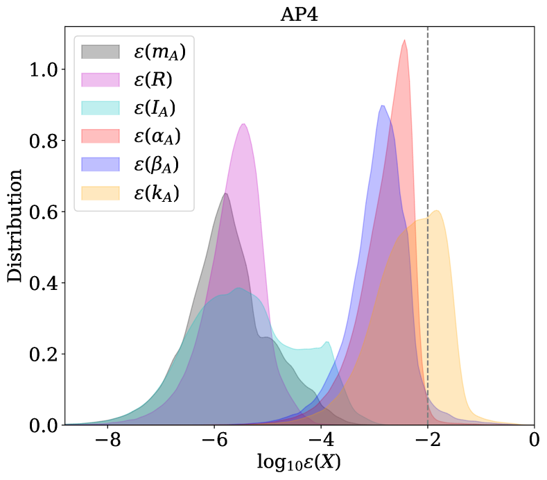
where $X\in\{m_{A},R,I_{A},\alpha_{A},\beta_{A},k_{A}\}$, to indicate the fractional accuracy of the ROMs. In Eq. (23), we denote $X_{\rm ROM}$ as the prediction of ROM, and $X_{\rm mTOV}$ as the value from solving the mTOV equations with the shooting algorithm. The values $X_{\rm mTOV}$ in the test space should also be calculated at different samples but with the same method to avoid the extra error induced by the use of different methods. Thus, instead of randomly generating parameters, we set another grid as the test space which is shifted from the training space for $\alpha_{0}$, $\beta_{0}$, and $\rho_{c}$, and calculate the parameters in the same way. The test space has the sparser distribution of $\beta_{0}$. Note that in this method we consider all errors for our ROMs, including the interpolating errors.

We show the distributions of $\varepsilon(X)$ in Fig. 5. The relative errors of $m_{A}$, $R$, and $I_{A}$ are sufficiently small to be $\lesssim 10^{-5}$. On the contrary, relative errors of $\alpha_{A}$, $\beta_{A}$, and $k_{A}$ are mostly smaller than 1%. Although their errors are larger than those of $R$, $m_{A}$, and $I_{A}$, the errors are, in most cases, still small enough to be neglected compared with the numerical errors from the shooting method. For $k_{A}$, in some cases the change of $I_{A}$ is rather small, as we have mentioned in Sec. III.1, leading to a relatively large numerical error when calculating the derivatives. Thus, a small fraction of prediction for $k_{A}$ in our ROM has a seemingly large error in the range $\sim 1$–$10\%$. However, we find that in such case we have $k_{A}\ll 1$, thus the deviation in this region has little influence on our study and will not have a practical effect.

Figure 6: Constraints on the DEF parameters $\left(\alpha_{0},\,\beta_{0}\right)$ from a variety of binary pulsars on the DEF theory with the EOS AP4. Regions above the curves are excluded, and the shaded area is the region that passes all tests in this plot. “Cassini” stands for the upper limit from the Shapiro time-delay measurement in the Solar System Bertotti et al. (2003). Timing of binary pulsars provides constraints in strong field regime where $\beta_{0}\lesssim-4.0$.

Figure 7: Similar to Fig. 6, but with projected limits from aLIGO, CE and ET with hypothetical GW signals of BNSs at a distance of 200 Mpc. The dashed lines represent the constraints from a $\left(1.25\,\mathrm{M_{\odot}},\,1.6\,\mathrm{M_{\odot}}\right)$ BNS merger event, and the dotted lines correspond to a $\left(1.25\,\mathrm{M_{\odot}},\,2.0\,\mathrm{M_{\odot}}\right)$ event. The shaded area is an illustration for combining all these constraints. We plot the limits from PSR J1738$+$0333 and the Cassini mission for comparison.

Table 1: Binary parameters of the five NS-WD systems that we use to constrain the DEF theory (PSRs J0348$+$0432 Antoniadis et al. (2013), J1012$+$5307 Lazaridis et al. (2009); Desvignes et al. (2016); Antoniadis et al. (2016); Mata Sánchez et al. (2020), J1738$+$0333 Freire et al. (2012), J1909$-$3744 Liu et al. (2020b), and J2222$-$0137 Cognard et al. (2017)). The intrinsic time derivatives of the orbit period, $\dot{P}_{b}^{\rm int}$, are derived from $\dot{P}_{b}^{\rm obs}$ by subtracting the acceleration effect Damour and Taylor (1991) and other kinematic effects such as the “Shklovskii” effect Shklovskii (1970). The Galactic acceleration effect is obtained from the latest Galactic potential model in Ref. McMillan (2017). For PSRs J0348$+$0432, J1012$+$5307, and J1738$+$0333, the pulsar masses, $m_{A}^{\mathrm{obs}}$, are obtained from the companion masses, $m_{B}^{\mathrm{obs}}$, and mass ratios, $q$. For PSRs J1909$-$3744 and J2222$-$0137, the masses are calculated from the Shapiro delay Shao et al. (2017). We list the standard $1$-$\sigma$ errors in units of the least significant digit(s) in parentheses.

Name	J0348$+$0432	J1012$+$5307	J1738$+$0333	J1909$-$3744	J2222$-$0137
Orbital period, $P_{b}\,({\rm d})$	0.102424062722(7)	0.60467271355(3)	0.3547907398724(13)	1.533449474305(5)	2.44576454(18)
Eccentricity, $e$	0.0000026(9)	0.0000012(3)	0.00000034(11)	0.000000115(7)	0.00038096(4)
Observed $\dot{P}_{b}$, $\dot{P}_{b}^{\rm obs}\,({\rm fs\,s^{-1}})$	$-273(45)$	50(14)	$-17.0(31)$	$-510.87(13)$	200(90)
Intrinsic $\dot{P}_{b}$, $\dot{P}_{b}^{\rm int}\,({\rm fs\,s^{-1}})$	$-274(45)$	$-5(9)$	$-27.72(64)$	$-4.4(79)$	$-60(90)$
Periastron advance, $\dot{\omega}\,({\rm deg\,yr^{-1}})$	—	—	—	—	0.1001(35)
Einstein delay $\gamma\,({\rm ms})$	—	—	—	—	—
Pulsar mass, $m_{A}^{\mathrm{obs}}\,({\rm M_{\odot}})$	—	—	—	1.492(14)	1.76(6)
Companion mass, $m_{B}^{\mathrm{obs}}\,({\rm M_{\odot}})$	$0.1715_{-0.0030}^{+0.0045}$	0.174(7)	$0.1817_{-0.0054}^{+0.0073}$	0.209(1)	1.293(25)
Mass ratio, $q\equiv m_{A}/m_{B}$	11.70(13)	10.5(5)	8.1(2)	—	—

Table 2: Binary parameters of the three NS-NS systems that we use to constrain the DEF theory (PSRs B1913$+$16 Weisberg and Huang (2016), J0737$-$3039A Kramer et al. (2006), and J1757$-$1854 Cameron et al. (2018)). For PSR B1913$+$16, the masses are determined from measurement of periastron advance, $\dot{\omega}$, and Einstein delay, $\gamma$. For PSR J0737$-$3039A, the masses are determined from the measurement of $\dot{\omega}$ and theory-independent mass ratio $q$. For PSR J1757$-$1854, the masses are derived from DDGR model. Similar to Table 1, we list the standard $1$-$\sigma$ errors in units of the least significant digit(s) in parentheses.

Name	B1913$+$16	J0737$-$3039A	J1757$-$1854
Orbital period, $P_{b}\,({\rm d})$	0.322997448918(3)	0.10225156248(5)	0.18353783587(5)
Eccentricity, $e$	0.6171340(4)	0.0877775(9)	0.6058142(10)
Observed $\dot{P}_{b}$, $\dot{P}_{b}^{\rm obs}\,({\rm fs\,s^{-1}})$	$-2423(1)$	$-1252(17)$	$-5300(200)$
Intrinsic $\dot{P}_{b}$, $\dot{P}_{b}^{\rm int}\,({\rm fs\,s^{-1}})$	$-2398(4)$	$-1252(17)$	$-5300(240)$
Periastron advance, $\dot{\omega}\,({\rm deg\,yr^{-1}})$	4.226585(4)	16.89947(68)	10.3651(2)
Einstein delay $\gamma\,({\rm ms})$	4.307(4)	0.3856(26)	3.587(12)
Pulsar mass, $m_{A}^{\mathrm{obs}}\,({\rm M_{\odot}})$	1.438(1)	1.3381(7)	1.3384(9)
Companion mass, $m_{B}^{\mathrm{obs}}\,({\rm M_{\odot}})$	1.390(1)	1.2489(7)	1.3946(9)
Mass ratio, $q\equiv m_{A}/m_{B}$	—	1.0714(11)	—

IV Constraints from binary pulsars

Constraints on the DEF parameters, $\alpha_{0}$ and $\beta_{0}$, have been investigated from various gravitational systems. In the Solar System, the Cassini mission Bertotti et al. (2003) places a constraint on $\alpha_{0}$, $|\alpha_{0}|<3.4\times 10^{-3}$ at at $1$-$\sigma$ uncertainty, from the measurement of Shapiro delay in the weak-field regime. In the strong-field regime, timing of binary pulsars provides the most stringent constraints so far to the DEF theory Damour and Esposito-Farèse (1996); Antoniadis et al. (2013); Freire et al. (2012); Shao et al. (2017); Anderson et al. (2019). Here we extend the analysis in Refs. Shao et al. (2017); Zhao et al. (2019), by carefully selecting more systems and constraining the DEF parameters in a numerically faster and reliable way with the ROMs we built in Sec. III. We employ the MCMC technique Foreman-Mackey et al. (2013); Shao et al. (2017) to derive constraints by combining the timing observations from binary pulsar systems, including NS-WD and NS-NS systems. We also discuss the improvements on deriving NS properties and the constraints on the DEF parameters.

IV.1 Setup

Previous work Shao et al. (2017); Zhao et al. (2019) has constrained the spontaneous scalarization of the DEF theory via MCMC simulations by combining observations of the PPK parameter $\dot{P}_{b}$ of some well-timed binary pulsars. These previous studies considered five well-timed NS-WD binary pulsars, PSRs J0348$+$0432 Antoniadis et al. (2013), J1012$+$5307 Lazaridis et al. (2009); Desvignes et al. (2016); Antoniadis et al. (2016); Mata Sánchez et al. (2020), J1738$+$0333 Freire et al. (2012), J1909$-$3744 Liu et al. (2020b), and J2222$-$0137 Cognard et al. (2017). We include these five systems in our study as well and their latest relevant parameters are listed in Table 1. For these systems, WD companions are weakly self-gravitating objects, leading to a tiny effective scalar coupling $\alpha_{B}\approx\alpha_{0}$. It indicates a large dipolar contribution $\propto(\alpha_{A}-\alpha_{0})^{2}$ to $\dot{P}_{b}$, if $\alpha_{A}$ is sufficiently different from $\alpha_{0}$ [see Eq. (9)]. As explained in the caption of Table 1, the measurements of the masses are independent of the PPK parameter $\dot{P}_{b}$. Thus, we can safely place bounds on the parameters of the DEF theory by utilizing these masses and the intrinsic orbital decay rate, $\dot{P}_{b}^{\mathrm{int}}$.

Apart from the five NS-WD systems, we add three NS-NS systems in our study. As discussed above, due to the closeness of $\alpha_{A}$ and $\alpha_{B}$, the dipolar radiation of these (almost) symmetric double NS systems is small, making it difficult to constrain the DEF theory with $\dot{P}_{b}$. However, as shown in Sec. II, some other PPK parameters derived from pulsar timing, such as the periastron advance rate $\dot{\omega}$ and the Einstein delay parameter $\gamma$, are also modified in the DEF theory. These modifications are considerable, especially for NS-NS binaries. Therefore, these double NS systems are potentially powerful laboratories to constrain the free parameters of the DEF theory. In Table 2, we show parameters of three well-timed double NSs used in this study: PSRs B1913$+$16 Weisberg and Huang (2016), J0737$-$3039A Kramer et al. (2006), and J1757$-$1854 Cameron et al. (2018). In these systems, the measurements of the masses depend on PPK parameters. For PSR B1913$+$16, the masses are determined from measurement of periastron advance, $\dot{\omega}$, and Einstein delay, $\gamma$. For PSR J0737$-$3039, the masses are determined from the measurement of $\dot{\omega}$ and theory-independent mass ratio $q$. For PSR J1757$-$1854, the masses are determined from the DDGR model Taylor (1987); Taylor and Weisberg (1989), which includes the contribution from all PPK parameters via their GR formats. In principle, only the independent subset of PPK parameters that were not used in deriving masses can be utilized to constrain the DEF parameters.

To obtain NSs’ properties, we need to assume a particular EOS. In this study, as mentioned earlier, we adopt 15 EOSs, namely AP3, AP4, BL_EOS, BSk20, BSk21, BSk22, BSk25, ENG, MPA1, PAL1, SLy4, SLy9, SLy230a, WFF1, and WFF2 (see Ref. Lattimer (2012) for a review). The mass-radius relations from these EOSs are shown in Fig. 1. These EOSs are all consistent with the observed $2\,\mathrm{M_{\odot}}$ maximum mass limit of NSs, and they are chosen inclined towards those which predict NS radius around $\sim 11$–$13\,\mathrm{km}$ for a mass of $1.4\,\mathrm{M_{\odot}}$, as favored by the tidal deformability measurement in GW170817 Abbott et al. (2017b); De et al. (2018); Capano et al. (2020).

IV.2 Constraints from individual pulsars

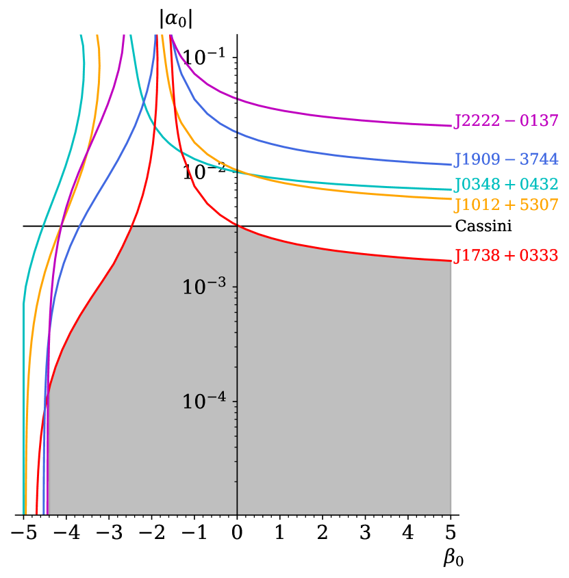
Before the MCMC simulations, we can estimate the constraints on the DEF parameters, $\alpha_{0}$ and $\beta_{0}$, from individual binary systems. We saturate the uncertainties on individual PPK parameters to determine the upper limits of the DEF parameters. By determining if the predicted value $\dot{P}_{b}^{\mathrm{th}}$ from Eqs. (9) and (10) lies within the $2$-$\sigma$ range of $\dot{P}_{b}^{\rm int}$, i.e., $\dot{P}_{b}^{\rm int}\pm 2\delta\dot{P}_{b}^{\rm int}$, we obtain the limits on the difference of effective scalar couplings $\alpha_{A}$ and $\alpha_{B}$, i.e., $|\Delta\alpha|=\left|\alpha_{A}-\alpha_{B}\right|$. With it, we constrain parameters $\alpha_{0}$ and $\beta_{0}$.

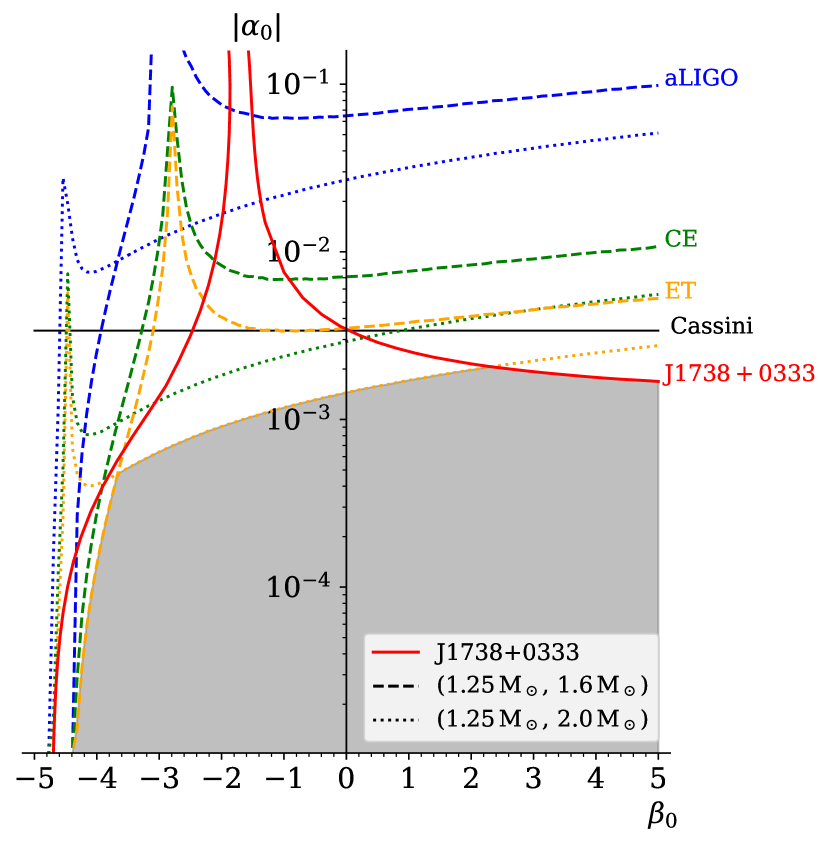
In Fig. 6, we show the constraints on $\alpha_{0}$ and $\beta_{0}$ obtained from binary pulsars. In these systems, PSR J1738$+$0333 gives almost the most stringent constraint. The upper limit of $\beta_{0}$ can reach $\sim-4.4$ from PSRs J1012+5307 and J2222$-$0137. When $\beta_{0}$ is around $-3$ to $-2$, the constraints from binary pulsars are weak, leading to a peak of $|\alpha_{0}|$. However, the limit from the Cassini mission helps exclude this region. In Fig. 7, we show constraints from hypothetical asymmetric BNS merger events at 200 Mpc, to be probed by GW detectors including Advanced LIGO (aLIGO), CE, and ET Shao et al. (2017). We assume two hypothetical BNSs with masses, $(1.25\,\mathrm{M_{\odot}},\,1.6\,\mathrm{M_{\odot}})$ and $(1.25\,\mathrm{M_{\odot}},\,2.0\,\mathrm{M_{\odot}})$, and the limits are obtained from Fisher information matrix Finn (1992). It is shown that the GW detectors could help in constraining the DEF parameters if such BNSs are observed. Among the three detectors, ET would probably provide tighter bounds, due to its lower starting frequency. Note that these constraints are dependent on the specific EOS, and in Figs. 6 and 7 we have assumed EOS AP4. The results are similar to previous results in Refs. Freire et al. (2012); Shao et al. (2017).

IV.3 The Bayesian inference and the MCMC framework

We here explore the constraints on the DEF theory combining the well-timed binary pulsars through MCMC simulations. MCMC technique provides a convenient and statistically sound algorithm to generate the distribution of unknown parameters for a model with many free parameters. In this study, we use EMCEE, a python implementation of an affine-invariant MCMC ensemble sampler, and our pySTGROMX package to speed up the calculation within the Bayesian framework.

In the Bayesian inference, given priors, hypothesis $\mathcal{H}$, data $\mathcal{D}$, and all the extra relevant information $\mathcal{I}$, the posterior distribution of the DEF parameters ($\alpha_{0}$, $\beta_{0}$), $P(\alpha_{0},\beta_{0}|\mathcal{D},\mathcal{H},\mathcal{I})$, can be inferred by

$$P(\alpha_{0},\beta_{0}|\mathcal{D} ,\mathcal{H},\mathcal{I})=$$

$$\int\frac{P(\mathcal{D}|\alpha_{0},\beta_{0},\bm{\Xi},\mathcal{H},\mathcal{I})P(\alpha_{0},\beta_{0},\bm{\Xi}|\mathcal{H},\mathcal{I})}{P(\mathcal{D}|\mathcal{H},\mathcal{I})}\differential\bm{\Xi}\,,$$

where $\bm{\Xi}$ denotes all the extra unknown parameters in the theory. In Eq. (IV.3), $P(\mathcal{D}|\alpha_{0},\beta_{0},\bm{\Xi},\mathcal{H},\mathcal{I})$ is the likelihood function, $P(\alpha_{0},\beta_{0},\bm{\Xi}|\mathcal{H},\mathcal{I})$ the prior, and

$$P(\mathcal{D}|\mathcal{H},\mathcal{I})=\int P(\mathcal{D}|\bm{\Xi},\mathcal{H},\mathcal{I})P(\bm{\Xi}|\mathcal{H},\mathcal{I})\differential\bm{\Xi}\,,$$ (25)

the model evidence which merely plays a role of normalization here Del Pozzo and Vecchio (2016). Based on Eq. (IV.3), MCMC method generates a sampling of values $(\alpha_{0},\,\beta_{0})$ that satisfies the posterior distribution.

In the MCMC simulations, the parameters, $\alpha_{0}$ and $\beta_{0}$, are constrained by evaluating the likelihood function. Considering all the binary pulsar systems we include, we use a general logarithmic likelihood function,

$$\ln\mathcal{L}_{\mathrm{PSR}} = -\frac{1}{2}\sum_{i=1}^{N_{\mathrm{PSR}}}\left[\left(\frac{\dot{P}_{b}-\dot{P}_{b}^{\mathrm{int}}}{\sigma_{\dot{P}_{b}^{\mathrm{int}}}}\right)^{2}+\left(\frac{\dot{\omega}-\dot{\omega}^{\mathrm{obs}}}{\sigma_{\dot{\omega}^{\mathrm{obs}}}}\right)^{2}+\left(\frac{\gamma-\gamma^{\mathrm{obs}}}{\sigma_{\gamma^{\mathrm{obs}}}}\right)^{2}\right.$$ (26)

$$\left.+\left(\frac{m_{A}-m_{A}^{\mathrm{obs}}}{\sigma_{m_{A}^{\mathrm{obs}}}}\right)^{2}+\left(\frac{m_{B}-m_{B}^{\mathrm{obs}}}{\sigma_{m_{B}^{\mathrm{obs}}}}\right)^{2}\right]_{i}\,,$$

for $N_{\mathrm{PSR}}$ binary pulsars. Here we assume that observations of different binary pulsars are independent. The intrinsic orbital decay $\dot{P}_{b}^{\mathrm{int}}$, the periastron advance rate $\dot{\omega}^{\mathrm{obs}}$, the Einstein delay parameter $\gamma^{\mathrm{obs}}$, the pulsar mass $m_{A}^{\mathrm{obs}}$, and the companion mass $m_{B}^{\mathrm{obs}}$ are given in Tables 1 and 2. Their observational $1$-$\sigma$ uncertainties are denoted as $\sigma_{X}$, where $X\in\left\{\dot{P}_{b}^{\mathrm{int}},\dot{\omega}^{\mathrm{obs}},\gamma^{\mathrm{obs}},m_{A}^{\mathrm{obs}},m_{B}^{\mathrm{obs}}\right\}$. The parameters, $\dot{P}_{b}$, $\dot{\omega}$, $\gamma$, and $m_{A}$ are dependent on the parameter set, $(\alpha_{0},\beta_{0},\bm{\Xi})$. The companion mass $m_{B}$ is consistently given from the parameter set $(\alpha_{0},\beta_{0},\bm{\Xi})$ as well when it is a NS. Otherwise, for a WD, it is generated randomly within the $1$-$\sigma$ uncertainty of $m_{B}^{\mathrm{obs}}$.

For WD companions, the coupling parameters can be reduced to $\alpha_{B}=\alpha_{0}$ and $\beta_{B}=\beta_{0}$. Thus, their contributions to $\dot{\omega}$ and $\gamma$ can be neglected. In addition to the five NS-WD binary pulsars that have been investigated in Refs. Shao et al. (2017); Zhao et al. (2019), we combine three extra double NS systems. In these NS-NS systems, we could utilize the information from $\dot{\omega}$ and $\gamma$. However, not each pulsar’s measurements of $\dot{\omega}$, $\gamma$, $m_{A}$, and $m_{B}$ are independent, as we have mentioned above. Thus, only for some suitable pulsar systems, the contributions of $\dot{\omega}$ and $\gamma$ are counted in a consistent way. In this study, we combine the contributions from $\dot{P}_{b}^{\mathrm{int}}$ of eight binary pulsars and $\gamma$ of PSR J0737$-$3039A in total for our estimation. In this way, we utilize the available information from the timing data as much as possible.

Note that the other parameters included in MCMC calculations, such as the orbital period, $P_{b}$, and the orbital eccentricity, $e$, are well-measured from the observations (see Tables 1 and 2). Thus, it is sufficient to adopt their central values for simplicity in the process of MCMC calculations.

In the MCMC calculation, the information we utilize to constrain the parameter space of $\left(\alpha_{0},\beta_{0}\right)$ is from the NSs. In total, we have $N=N_{\mathrm{NS-WD}}+2N_{\mathrm{NS-NS}}$ NSs from the observations. To describe the observational signatures fully in the DEF theory, we need $N+2$ free parameters, collectively denoted as $\bm{\theta}=\left\{\alpha_{0},\,\beta_{0},\,\rho_{c}^{(i)}\,(i=1,2,...,N)\right\}$ where $\rho_{c}^{(i)}$ is the central matter density of NS $i$ in the Jordan frame. The initial values of $\rho_{c}^{(i)}$ are sampled around their GR values. We allow the simulation to explore a large region of central matter density. Thanks to our ROMs, the initial central values of the scalar field $\varphi_{c}$ are no longer needed during the calculation, which avoids extra computationally intensive calculations Shao et al. (2017). Using $\alpha_{0}$, $\beta_{0}$, and $\rho_{c}^{(i)}$, we obtain the properties of NSs. Then we calculate the PPK parameters and the log-likelihood functions to evaluate the posteriors.

In this study, we carefully choose the priors of $(\alpha_{0},\,\beta_{0})$ to cover the region of interest where the spontaneous scalarization develops. For each MCMC run, we assume a uniform prior distribution of $\left(\log_{10}|\alpha_{0}|,\,\beta_{0}\right)$ in the region of our ROMs, i.e., $\left(\log_{10}|\alpha_{0}|,\,\beta_{0}\right)\in[-5.3,-2.5]\times[-4.8,-4.0]$.

For each MCMC simulation, we use 32 walkers (chains) and 100,000 steps for each walker. Thus, we produce 3.2 million samples in total. The last half chain samples are remained and “thined”, with a thinning factor of ten, to reduce dependence on the initial values and correlation of the adjacent samples Foreman-Mackey et al. (2013); Gelman and Rubin (1992). We perform the Gelman-Rubin test for convergence, and we have confirmed that our samples pass the test Gelman and Rubin (1992). Thus, our posteriors of $\alpha_{0}$ and $\beta_{0}$ are statistically reliable. We end up with $1.6\times 10^{5}$ “thinned” samples for each simulation to infer the marginalized distributions of the free parameters $\alpha_{0}$ and $\beta_{0}$. Eventually, we apply this procedure to all the 15 EOSs.

Figure 8: Marginalized 2-d posteriors distribution for $\left(\log_{10}|\alpha_{0}|,-\beta_{0}\right)$ from MCMC runs on the eight pulsars listed in Tables 1 and 2 with the EOS AP4. The marginalized 1-d distributions and the corresponding upper limits at 68% CL and 90% CL are illustrated in upper and right panels.

Figure 9: Similar to Fig. 8, but for all the 15 EOSs. The marginalized 1-d distributions and the upper limits at 68% CL and 90% CL are illustrated in upper and right subpanels of each panel.

Figure 10: Violin plots of the marginalized 1-d posterior distributions in the parameter space of $\log_{10}|\alpha_{0}|$ (upper panel) and $-\beta_{0}$ (lower panel) for 15 EOSs in our study. The 90% and 68% CL upper bounds are shown by the black and blue markers, respectively.

Figure 11: The upper bounds at 90% CL on the NS effective scalar coupling parameters, $\alpha_{A}$, $\beta_{A}$, and $k_{A}$, considering the combined constraints from the five NS-WD pulsars in Table 1 and three NS-NS pulsars in Table 2.

IV.4 Constraints from combining binary pulsars

We here show the constraints from the timing measurements of binary pulsars from the application of our ROMs. To achieve the speedups of MCMC calculations, we restrict the priors of $\log_{10}|\alpha_{0}|$ and $\beta_{0}$ to the same ranges as in our ROMs. With the MCMC simulations done, we can obtain the posterior distributions of the DEF parameters $\log_{10}|\alpha_{0}|$ and $\beta_{0}$ for the 15 EOSs we adopt.

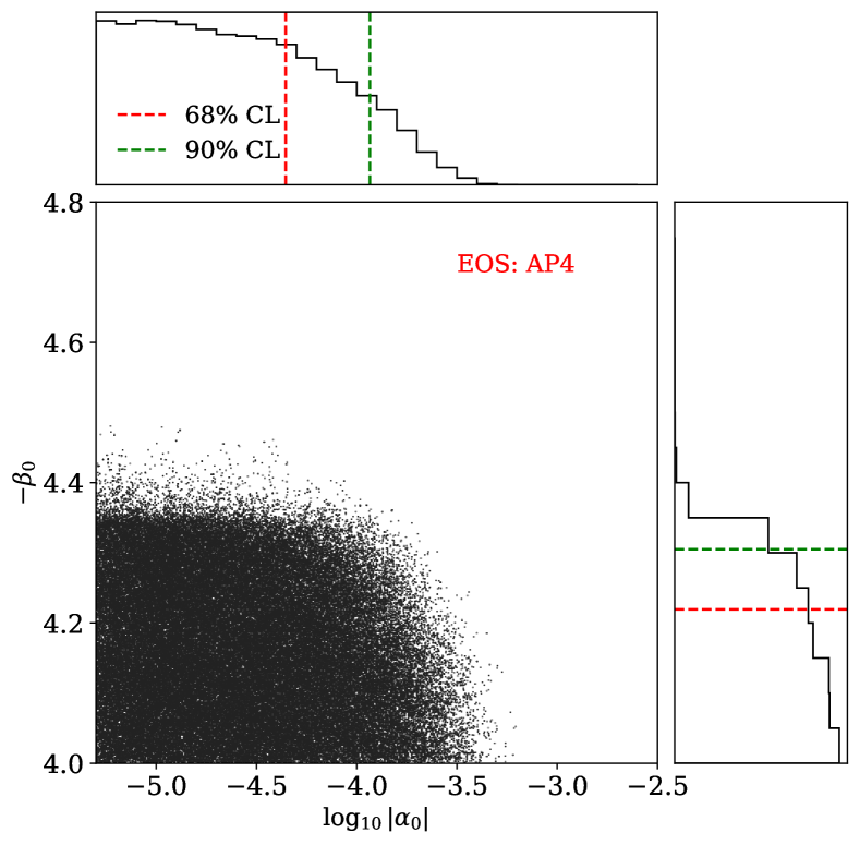
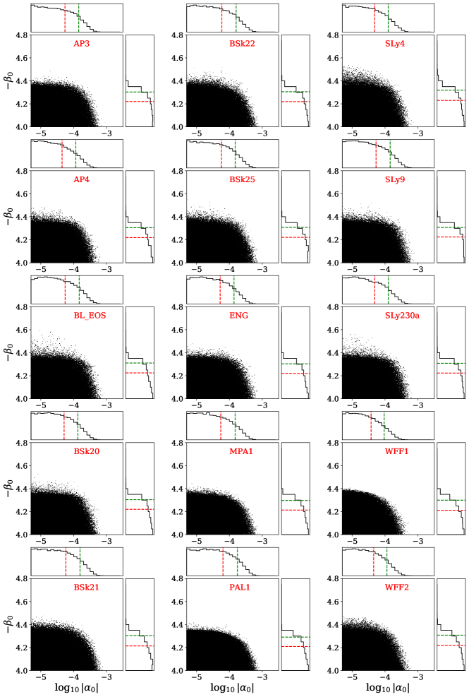
In Fig. 8, as an example, we show the marginalized 2-dimensional (2-d) and 1-d posterior distributions in the parameter space of $\left(\log_{10}|\alpha_{0}|,\,-\beta_{0}\right)$ and the constraints at 68% and 90% confidence levels (CLs) for EOS AP4. As mentioned above, the priors of $\left(\log_{10}|\alpha_{0}|,\,-\beta_{0}\right)$ are uniform distributions in the rectangle region of Fig. 8. The results from pulsars provide very tight constraints on the parameters of the DEF theory. The upper limits of $\log_{10}|\alpha_{0}|$ and $-\beta_{0}$ are constrained to $\sim-3.9$ and $\sim 4.3$ at 90% CL, respectively. The constraints are overall similar to previous results from Refs. Zhao et al. (2019); Shao et al. (2017). The extra double NS systems provide certain but not remarkable improvements in our results. The tight constraints are mainly contributed by the dipolar radiation in the NS-WD systems. Here, we mainly aim to provide a test that proves the ability of our method to constrain these parameters. In the future, with the further precise observations of binary pulsars, the PPK parameters $\dot{\omega}$ and $\gamma$ might provide additional constraints for the DEF gravity.

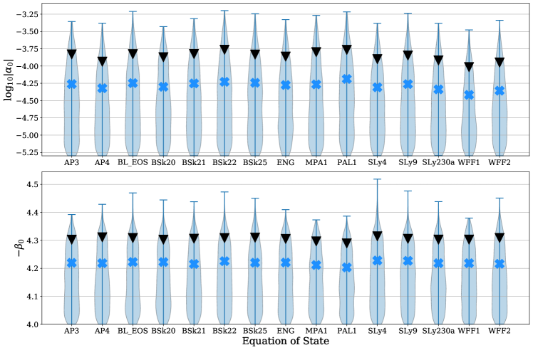
We apply the analysis above to all the 15 EOSs. The marginalized 2-d and 1-d distributions from the MCMC results for all the 15 EOSs we include in this study are shown in Fig. 9. In addition, in Fig. 10 we show the 1-d distributions of $\log_{10}|\alpha_{0}|$ and $-\beta_{0}$, and their upper bounds at 68% and 90% CLs for all the EOSs. These results are overall similar, but show the dependence on the choice of EOS. The upper bounds on $\alpha_{0}$ at 90% CL are approximately $10^{-4}$. The upper bounds on $-\beta_{0}$ at 90% CL are $\sim 4.3$.

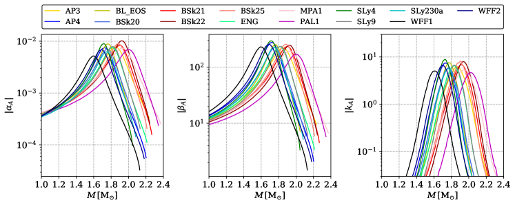
Using our ROMs, we can conveniently discuss the spontaneous scalarization phenomena of a NS. In Fig. 11, we illustrate the upper bounds at 90% CL on the absolute values of coupling parameters: effective scalar coupling $\alpha_{A}$ and its derivative, $\beta_{A}$, as well as coupling factor for the moment of inertial, $k_{A}$, as functions of the NS mass, $m_{A}$. The ranges below the curves mark the regions that are unconstrained up to now. It is shown clearly that, for all the 15 EOSs, the allowed maximum values of these parameters are constrained tightly. In left panel of Fig. 11, the upper bounds at 90% CL on the NSs show that for some EOSs, the maximal effective scalar coupling allowed is $\sim 10^{-2}$. A remarkable scalarization of NS at this level is still permitted for a NS with a suitable mass within the range of $1.6$–$2.0\,\mathrm{M_{\odot}}$. Compared with earlier results Shao et al. (2017); Zhao et al. (2019), the “scalarization window” is still open though slightly limited further. An improvement in this study is that, besides the scalar coupling $\alpha_{A}$, we can investigate the coupling parameters $\beta_{A}$ and $k_{A}$ conveniently with our ROMs. As shown in the middle and right panels of Fig. 11, the peaks with extremely large values of $\beta_{A}$ and $k_{A}$ shown in Fig. 3 due to the fact of strong scalarization are essentially ruled out. Only mild deviation is permitted now. The maximum values are $\sim 3\times 10^{2}$ for $\left|\beta_{A}\right|$ and $\sim 10$ for $\left|k_{A}\right|$. Therefore, a very large deviation of these scalar coupling parameters from GR is not expected based on the contemporary observation. However, there is still some room for a noteworthy spontaneous scalarization.

In addition, we note that for a stiffer EOS, spontaneous scalarization tends to be significant for larger mass, from $1.4$–$1.7\,\mathrm{M_{\odot}}$ (EOS WFF1) to $1.8$–$2.2\,\mathrm{M_{\odot}}$ (EOS PAL1). Most of the NS masses in our study lie in $m_{A}\sim 1.3$–$1.7\,\mathrm{M_{\odot}}$. As a consequence, the MCMC simulation shows that, the tightest constraint is obtained for EOS WFF1.

To summarize, we provide a quick and statistically reliable method to constrain the DEF parameters. We verify the validity of the method and give the stringent constraints on the DEF theory. The bounds are slightly improved, but overall similar to previous studies Zhao et al. (2019); Shao et al. (2017). Constraints on $|\alpha_{0}|$ and $\beta_{0}$ depend on the precision of the observation, choice of pulsar systems, EOSs, and priors. The “scalarization window” is still open at the level of $\sim 10^{-2}$ for all the EOSs. More observations and suitable systems in the future, such as possible observations of pulsar timing and GWs from BNSs with NS masses lying in the “scalarization window”, will help to place new constraints on the DEF theory.

V Conclusion

This work studies the DEF theory that predicts large deviations from GR for NSs through nonperturbative spontaneous scalarization phenomena. We briefly review the scalarization phenomena of the DEF theory and relevant predictions. To avoid solving the mTOV equations for slowly rotating NSs repeatedly, which is time-consuming and computationally expensive, we construct efficient ROMs to derive NSs’ properties including $m_{A}$, $R$, $I_{A}$, $\alpha_{A}$, $\beta_{A}$, and $k_{A}$ for the DEF theory, extending earlier work. Based on the contemporary observations about the properties of NSs, such as masses and radii, we build ROMs for 15 carefully selected EOSs. The ROMs for our calculations are coded in a python package pySTGROMX and made public for the community use. After testing the performance of the ROMs, we find that, compared with the shooting algorithm, our ROMs can speed up the relevant calculations by two orders of magnitude for $\alpha_{A}$ and even three orders for $\beta_{A}$ and $k_{A}$, and yet still keep accuracy at $\sim 1\%$ level. This extended model gives an accurate and more comprehensive description of NSs’ properties in the DEF gravity.

As an application, we utilize pySTGROMX to explore constraints on the DEF theory with well-timed binary pulsars through MCMC simulations. We use the latest precise data from five NS-WD systems and three NS-NS systems, to derive tight constraint of the DEF theory. We constrain the DEF parameters to be $|\alpha_{0}|\lesssim 10^{-3.9}$ and $-\beta_{0}\lesssim 4.3$ at the 90% CL for a variety of EOSs. The constraints are dependent on the precision of the observation, choice of pulsar systems, priors, and EOSs. We find that the “scalarization window” still exists at $\sim 10^{-2}$ level. In the future, if NSs whose masses lie around the “scalarization window” can be observed precisely, the possibility of a strong scalarization for NSs may be excluded entirely.

In the future, we note that the new large radio telescopes, e.g., the Five-hundred-meter Aperture Spherical radio Telescope (FAST) Nan et al. (2011) and the Square Kilometre Array (SKA) Kramer et al. (2004); Shao et al. (2015), are expected to improve the precision of pulsar timing and also to discover new pulsar systems, especially NS-NS systems. These would help to close the “scalarization window”. Furthermore, the current and next-generation GW detectors, such as the aLIGO, CE, ET, and KAGRA, could have more detection of compact binary coalescences in the future. These observations would provide more information to be used to investigate alternative theories of gravity in a more precise and accurate way. Our ROMs are constructed for quick and sound evaluation of the parameters in the DEF theory, suitable for applications for binary pulsar experiments, as well as GWs to some extent.